Wasserstein-based Kernels for Clustering: Application to Power Distribution Graphs

Abstract

Many data clustering applications must handle objects that cannot be represented as vector data. In this context, the bag-of-vectors representation can be leveraged to describe complex objects through discrete distributions, and the Wasserstein distance can effectively measure the dissimilarity between them. Additionally, kernel methods can be used to embed data into feature spaces that are easier to analyze. Despite significant progress in data clustering, a method that simultaneously accounts for distributional and vectorial dissimilarity measures is still lacking. To tackle this gap, this work explores kernel methods and Wasserstein distance metrics to develop a computationally tractable clustering framework. The compositional properties of kernels allow the simultaneous handling of different metrics, enabling the integration of both vectors and discrete distributions for object representation. This approach is flexible enough to be applied in various domains, such as graph analysis and image processing. The framework consists of three main components. First, we efficiently approximate pairwise Wasserstein distances using multiple reference distributions. Second, we employ kernel functions based on Wasserstein distances and present ways of composing kernels to express different types of information. Finally, we use the kernels to cluster data and evaluate the quality of the results using scalable and distance-agnostic validity indices. A case study involving two datasets of 879 and 34,920 power distribution graphs demonstrates the framework’s effectiveness and efficiency.

[RRE]organization=Reliability and Risk Engineering Lab, Institute of Energy and Process Engineering, Department of Mechanical and Process Engineering, ETH Zurich, country=Switzerland

1 Introduction

Data clustering is a fundamental problem in data science, and thus has attracted considerable attention. The goal of data clustering is to group similar objects into clusters while separating dissimilar ones into distinct clusters [1]. However, the intricacies associated with clustering pose relevant challenges. One challenge is defining the permissible cluster shapes, especially in datasets with diverse and complex structures. Additionally, clustering requires a suitable notion of similarity that aligns with the dataset’s characteristics [2]. As data clustering advances to complex objects, the quest for solutions to these challenges continues, prompting ongoing research.

One common approach to clustering involves learning a set of prototype objects to minimize a function based on the distances between clustered objects and their respective prototypes. This approach gave rise to the popular k-means [3] and k-medoids [4] algorithms. k-means uses centroids as prototypes, while k-medoids employs medoids. These algorithms have been predominantly applied to vector spaces. However, many machine learning tasks require the analysis of non-vectorial datasets, such as in electroencephalography signal processing [5] and image texture recognition [6].

Adaptations of k-means and k-medoids have been developed for non-vectorial settings. [7] extends the k-means algorithm to the Riemannian manifold of symmetric positive definite (SPD) matrices. In [8], the authors introduce a fast k-medoids clustering method for the same manifold. Moreover, [6] broadens the kernel k-means application to the SPD matrices and Grassmann manifold. While these advancements expand the use of clustering techniques, the challenge of clustering bag-of-vectors, used for instance in image and graph analysis [9, 10], is not addressed. In the bag-of-vectors representation [11], the information from individual elements of objects, such as nodes in graphs or pixels in images, is portrayed with a vector. These vectors are then concatenated into a matrix representing the object, which is associated with a weight vector to denote the weight of each element. This type of representation is crucial in machine learning for portraying complex objects as it can be succinctly described through probability distributions [12].

The clustering of probability distributions is performed by leveraging Wasserstein distances and methods aiming to find prototypical distributions. The extension of k-means with Wasserstein distances gained significant attention since the work of [11]. As the exact computation of Wasserstein distances is expensive, various modifications have been proposed to alleviate its burden. In [12], the authors develop a modified Bregman alternating direction method of multipliers for computing approximate discrete Wasserstein barycenters. The work of [2] introduces a Wasserstein-based trimmed k-means that allows the trimming of the most discrepant distributions to improve computational performance and result robustness. A fast distribution clustering is introduced in [13], which uses a hybrid distance consisting of two terms. One term accounts for differences in expected values and covariances. The other term is a linear optimal transport approximation of the Wasserstein distance between distributions [9]. Despite significant progress in distribution clustering, investigating the adoption of kernel methods remains a promising avenue. This is due to their ability to unveil non-linear patterns in data [14] and their compositional properties for combining multiple similarity measures [15].

Kernel methods are well-established in machine learning due to their modeling capabilities [16]. Kernels enable the representation of dot products in high-dimensional feature spaces, facilitating data treatment and analysis [17]. Kernel methods have also been used to solve problems involving Wasserstein distances. For instance, [18] employs a support vector machine (SVM) classifier for graphs that uses an indefinite exponential kernel and the Fused Gromov-Wasserstein distance. Similarly, [10] constructs an SVM classifier for graphs with a positive definite Wasserstein Laplacian kernel over categorical data. Nevertheless, research in Wasserstein-based kernels has not yet addressed distribution clustering problems.

Clustering is a challenging task, and in most cases, it is not straightforward how to reach the best partition of the input data. Consequently, various validity indices have been proposed to compare cluster configurations [19, 20]. There is a clear distinction between external and internal validation based on the information available. External validation evaluates the partition quality against a correct and known partition, while internal validation only analyzes the clustered data. This work focuses on the latter since, in real applications, a correct partition of the data is unknown. Most internal validity indices consist of functions that measure cluster cohesion and cluster separation, such as the Davies-Bouldin index [21]. Additionally, information-theoretic measures allow for the identification of robust clustering solutions that exhibit small diversity under different initializations [22]. In the context of kernel clustering, solutions are often evaluated using external validity indices like Accuracy and Purity [23, 24]. However, internal validity indices that assess cluster shapes may not ensure the comparability of results, as kernel parameters alter the dissimilarities among data points. Furthermore, the intrinsic dimensionality of the feature space and the presence of outliers can significantly affect the values of these indices [25].

The scientific literature reveals three research gaps. First, no existing clustering method has provided a way of accounting for distributional and vectorial dissimilarity measures simultaneously. Second, computing Wasserstein distances between distributions imposes a significant bottleneck. Previous works have leveraged linear optimal transport methods to alleviate this burden [9, 26]. However, these methods rely on the selection of a single reference distribution to estimate pairwise distances. Consequently, distance approximations become sensitive to the choice of this reference. Finally, evaluating the quality of clustering solutions for data mapped in different spaces requires validity indices that do not directly depend on distance computations to ensure comparability. We refer to such indices as distance-agnostic. Current validity indices for assessing the appropriateness of cluster shapes are either not distance-agnostic or require extensive execution times.

This article develops a Wasserstein-based kernel framework for clustering that addresses the identified research gaps. It enables clustering objects represented by discrete distributions and vectors, which is common in domains such as graph analysis and image processing. The framework consists of three main components. First, we approximate pairwise Wasserstein distances between discrete distributions. Second, we utilize kernel functions based on Wasserstein distances, propose approaches to combine multiple kernels, and derive tractable mappings of the data. Lastly, we adopt a clustering method for the mapped data and introduce appropriate validity indices. The framework’s efficacy is evaluated through a power distribution graph data clustering application.

The main contributions of this article are as follows:

1. We develop a method to efficiently approximate pairwise Wasserstein distances using multiple reference distributions through linear optimal transport. This method reduces approximation errors and diminishes the impact of reference distribution selection compared to existing single-reference approaches, while also leveraging parallel computations.

2. We introduce a shifted exponential kernel based on Wasserstein distance computations. This type of kernel offers two main advantages: 1) it enables the detection of patterns that would otherwise be unobservable in the original space of the data, and 2) it can be composed with other kernels to simultaneously account for additional similarity measures. Moreover, we show that kernel principal component analysis (PCA) can be applied to reduce the impact of low-variance components on clustering solutions and adopt a suitable decomposition method for large datasets.

3. We propose an efficient and scalable distance-agnostic validity index that compares the quality of cluster shapes. This enables the analysis of clustering configurations across data mapped into different spaces. Our validity index, the Fast Goodman-Kruskal (FGK) index, is based on a sampling procedure to compute the Goodman-Kruskal index (GK) [27] on subsets of the analyzed data. This approach overcomes the scalability challenges of the original GK index and facilitates kernel parameter tuning when ground-truth clusters are unknown.

The remainder of this article is organized as follows. Section 2 develops the clustering framework. Section 3 provides the experimental setup of the power distribution graphs case study. Section 4 presents and analyzes the obtained clustering results. Section 5 discusses the strengths and limitations of the proposed framework. Finally, Section 6 gives concluding remarks.

2 Methodology

2.1 Wasserstein distances

In this section, we provide the necessary background on the Wasserstein distance and then introduce a method for its efficient pairwise computation.

The Wasserstein distance is a measure of the dissimilarity between two probability distributions. It quantifies the minimum transport cost needed to transform one probability distribution into the other. Consequently, it is suitable for comparing objects represented as distributions. Moreover, the Wasserstein distance based on Euclidean transport costs, is known to best reflect geometric features [28], e.g., Riemannian geometry aspects like geodesics and tangent spaces. The analytical definition of the Wasserstein distance with Euclidean transport costs between two probability distributions $\boldsymbol{\mu}_{i}$ and $\boldsymbol{\mu}_{j}$ defined on $\mathcal{X}\subseteq\mathbb{R}^{d}$, is [29]:

$$W(\boldsymbol{\mu}_{i},\boldsymbol{\mu}_{j})=\left(\inf_{\boldsymbol{\pi}\in\Pi(\boldsymbol{\mu}_{i},\boldsymbol{\mu}_{j})}\int_{\mathcal{X}\times\mathcal{X}}(||\boldsymbol{x}-\boldsymbol{y}||_{2})^{2}d\pi(\boldsymbol{x},\boldsymbol{y})\right)^{1/2}$$ (1)

where, $\mathcal{X}$ is a given normed vector space, $\Pi(\boldsymbol{\mu}_{i},\boldsymbol{\mu}_{j})$ denotes the set of all joint probability distributions, $\boldsymbol{\pi}$ is a joint distribution for $\boldsymbol{x}$ and $\boldsymbol{y}$ commonly referred to as a transport plan, and $(\boldsymbol{x},\boldsymbol{y})$ is any pair of points in $\mathcal{X}\times\mathcal{X}$. Given a pair $(\boldsymbol{x},\boldsymbol{y})$, the value of $\boldsymbol{\pi}(\boldsymbol{x},\boldsymbol{y})$ indicates the mass of $\boldsymbol{\mu}_{i}$ at $\boldsymbol{x}$ that is transported to $\boldsymbol{y}$ to reconstruct $\boldsymbol{\mu}_{j}$ from $\boldsymbol{\mu}_{i}$. The distance $W(\cdot,\cdot)$ in Eq. (1) is symmetric, nonnegative, satisfies the triangle inequality, and is finite when the second moments of both $\boldsymbol{\mu}_{i}$ and $\boldsymbol{\mu}_{j}$ exist.

Solving Eq. (1) is challenging, and closed-form solutions are available only when $\boldsymbol{\mu}_{i}$ and $\boldsymbol{\mu}_{j}$ belong to a location-scale family, such as Gaussian distributions [13]. If this condition is not met, the problem necessitates numerical solutions. Particularly, when $\boldsymbol{\mu}_{i}$ and $\boldsymbol{\mu}_{j}$ are discrete, the problem is reduced to solving an optimization model with a finite, possibly large, number of constraints and variables. In what follows, we delve into the discrete settings for solving Eq. (1).

2.1.1 Discrete setting

The Wasserstein distance between two discrete distributions $\boldsymbol{\mu}_{i}$ and $\boldsymbol{\mu}_{j}$ can be computed using optimal transport tools [12]. Consider two bag-of-vectors in $\mathbb{R}^{d}$, $\boldsymbol{X}=[\boldsymbol{x}^{m}]_{m=1}^{N^{\boldsymbol{\mu}_{i}}}$ and $\boldsymbol{Y}=[\boldsymbol{y}^{n}]_{n=1}^{N^{\boldsymbol{\mu}_{j}}}$, where $N^{\boldsymbol{\mu}_{i}}$ and $N^{\boldsymbol{\mu}_{j}}$ represent the number of vectors. The vectors in $\boldsymbol{X}$ and $\boldsymbol{Y}$ have positive probabilities $p_{m}$ and $q_{n}$ such that $\sum_{m}p_{m}=1$ and $\sum_{n}q_{n}=1$. We then define the discrete distributions supported on $\mathbb{R}^{d}$ as $\boldsymbol{\mu}_{i}=\sum_{m=1}^{N^{\boldsymbol{\mu}_{i}}}p_{m}\boldsymbol{\delta}_{\boldsymbol{x}^{m}}$ and $\boldsymbol{\mu}_{j}=\sum_{n=1}^{N^{\boldsymbol{\mu}_{j}}}q_{n}\boldsymbol{\delta}_{\boldsymbol{y}^{n}}$, where $\boldsymbol{\delta}_{\boldsymbol{x}^{m}}$ and $\boldsymbol{\delta}_{\boldsymbol{y}^{n}}$ are Dirac distributions at the locations $\boldsymbol{x}^{m}$ and $\boldsymbol{y}^{n}$, respectively. The Wasserstein distance between $\boldsymbol{\mu}_{i}$ and $\boldsymbol{\mu}_{j}$ can be obtained by solving the following linear program [11]:

$$W(\boldsymbol{\mu}_{i},\boldsymbol{\mu}_{j})^{2} =\min_{\boldsymbol{\pi}\geq\boldsymbol{0}}\sum_{m=1}^{N^{\boldsymbol{\mu}_{i}}}\sum_{n=1}^{N^{\boldsymbol{\mu}_{j}}}\pi_{mn}\left(||\boldsymbol{x}^{m}-\boldsymbol{y}^{n}||_{2}\right)^{2}$$ (2a)

$$\text{s.t.}\quad\sum_{m=1}^{N^{\boldsymbol{\mu}_{i}}} \pi_{mn}=q_{n}\quad\forall n=1,\ldots,N^{\boldsymbol{\mu}_{j}}\quad\text{;}\quad\sum_{n=1}^{N^{\boldsymbol{\mu}_{j}}}\pi_{mn}=p_{m}\quad\forall m=1,\ldots,N^{\boldsymbol{\mu}_{i}},$$ (2b)

where $\pi_{mn}$ is the matching weight between the support vectors $\boldsymbol{x}^{m}$ and $\boldsymbol{y}^{n}$. Hence, Eqs. (2a)-(2b) optimize the matching weights to minimize the sum of the transport costs to reconstruct $\boldsymbol{\mu}_{j}$ from $\boldsymbol{\mu}_{i}$. Although the problem is linear, its exact computation is challenging and scales at least as $\mathcal{O}(N^{3}\log(N))$ when comparing two distributions of $N$ support vectors [30]. Furthermore, consider a set of discrete distributions $\Delta=\{\boldsymbol{\mu}_{l}\}_{l=1}^{S}$, where each distribution $\boldsymbol{\mu}_{l}$ represents $\sum_{m=1}^{N^{\boldsymbol{\mu}_{l}}}p_{m}^{l}\boldsymbol{\delta}_{\boldsymbol{x}^{m,l}}$, with $\boldsymbol{x}^{m,l}$ being the $m$-th support vector of the $l$-th distribution, and $p_{m}^{l}$ is its corresponding probability. Computing the $S(S-1)/2$ pairwise Wasserstein distances for these $S$ distributions in $\Delta$ requires solving $S(S-1)/2$ optimization problems Eqs. (2a)-(2b) and becomes rapidly intractable. This motivates the exploration of approximate solutions.

2.1.2 Approximating pairwise Wasserstein distances

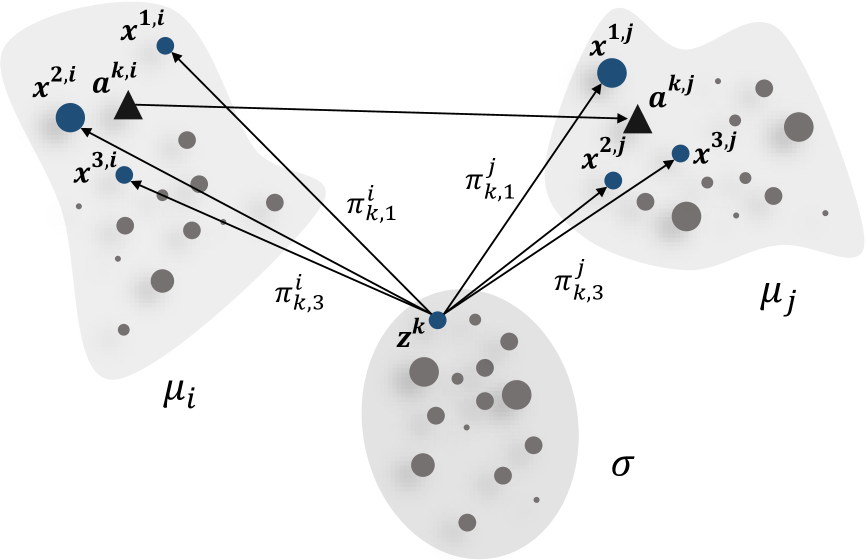
Figure 1: Illustration of the linear optimal transport distance variables. The reference $\boldsymbol{\sigma}$ is used to approximate the Wasserstein distance between the distributions $\boldsymbol{\mu}_{i}$ and $\boldsymbol{\mu}_{j}$.

Several works employ the concepts of the linear optimal transportation framework due to its computational efficiency and practical success [9, 26, 13]. This framework approximates pairwise Wasserstein distances between distributions in a set $\Delta$ using a reference distribution $\boldsymbol{\sigma}=\sum_{k=1}^{N^{\boldsymbol{\sigma}}}g_{k}\boldsymbol{\delta}_{\boldsymbol{z}^{k}}$. Given the reference distribution $\boldsymbol{\sigma}$, we compute $W(\boldsymbol{\mu}_{l},\boldsymbol{\sigma})$ with Eqs. (2a)-(2b) for every distribution in $\Delta$. The corresponding matching weights are used to compute the centroids of the mass transported from $\boldsymbol{z}^{k}$ to the distributions $\boldsymbol{\mu}_{l}$, respectively, which are referred to as forward images:

$$\boldsymbol{a}^{k,l}=\frac{1}{g_{k}}\sum_{m=1}^{N^{\boldsymbol{\mu}_{l}}}\pi_{k,m}^{l}\boldsymbol{x}^{m,l}\qquad\forall k=1,\ldots,N^{\boldsymbol{\sigma}},l=1,\ldots,S,$$ (3)

which are then used to compute pairwise distances in $\Delta$:

$$L_{\boldsymbol{\sigma}}(\boldsymbol{\mu}_{i},\boldsymbol{\mu}_{j})^{2}=\sum_{k=1}^{N^{\boldsymbol{\sigma}}}g_{k}\left(||\boldsymbol{a}^{k,i}-\boldsymbol{a}^{k,j}||_{2}\right)^{2}\qquad\forall(\boldsymbol{\mu}_{i},\boldsymbol{\mu}_{j})\in\Delta\times\Delta.$$ (4)

Fig. 1 provides a graphical depiction of Eq. (4), which approximates $W(\cdot,\cdot)$ between any two distributions in the set $\Delta$. This distance denotes the transport cost required to move the forward image of each supporting vector $\boldsymbol{z}^{k}$ in the reference $\boldsymbol{\sigma}$, projected in $\boldsymbol{\mu}_{i}$, to the forward image in $\boldsymbol{\mu}_{j}$. This approximation allows us to obtain the pairwise distances of the dataset $\Delta$ with $S$ distributions by solving only $S$ optimization problems Eqs. (2a)-(2b), instead of $S(S-1)/2$. This is because the forward images $\boldsymbol{a}^{k,l}$ in Eq. (3) are obtained through the computation of $W(\boldsymbol{\mu}_{l},\boldsymbol{\sigma})$ for $l=1,\ldots,S$. Then, the calculations described by Eq. (4) involve only weighted pairwise Euclidean distances.

2.1.3 Approximation using multiple reference distributions

A reference distribution far from the analyzed distributions worsens the distance approximation quality [9]. Different options have been considered in the literature: adopting a kernel density estimate of the combined distributions dataset [13], averaging the distributions and using particle approximation [9], applying k-means clustering to the combined support vectors of the discrete distributions, and sampling from a fitted normal distribution to obtain an empirical distribution [26]. Nevertheless, there is no method to determine the robustness of the distance approximation when choosing a reference [13].

Here, we develop a method that leverages multiple $R$ reference distributions. The method employs the following steps:

• Step 1 - Build an initial reference $\boldsymbol{\sigma}_{1}$: We stack the support vectors of the distributions in $\Delta$ into a matrix $\boldsymbol{X}^{S}$. Subsequently, k-means is applied on the weighted $\boldsymbol{X}^{S}$ to determine an initial reference $\boldsymbol{\sigma}_{1}$. The number of centroids is set to $\left\lfloor\frac{1}{S}\sum_{l=1}^{S}N^{\boldsymbol{\mu}_{l}}\right\rfloor$, which is the lower approximation of the average number of support vectors in $\Delta$. Using $\boldsymbol{\sigma}_{1}$, we compute the $S(S-1)/2$ pairwise distances $\boldsymbol{D}_{1}=\left[L_{\boldsymbol{\sigma}_{1}}(\boldsymbol{\mu}_{i},\boldsymbol{\mu}_{j})\right]_{i,j}$ in $\Delta$ via Eq. (4).

• Step 2 - Select additional references $\boldsymbol{\sigma}_{r}$: We select $R-1$ additional distributions in $\Delta$. This is done by clustering the distributions in $\Delta$ into $R-1$ clusters with k-medoids, using the distances $\boldsymbol{D}_{1}$. The medoids are the additional reference distributions, $\boldsymbol{\sigma}_{r}$, for $r=2,\ldots,R$.

Once the $R$ references have been selected, we compute all the pairwise distance matrices $\boldsymbol{D}_{r}$ corresponding to the distributions $\boldsymbol{\sigma}_{r}$ for $r=2,\dots,R$. Conveniently, the computation of the $\boldsymbol{D}_{r}$ matrices can be performed in parallel. Let $\Delta^{-}$ be the set defined as $\Delta\setminus\{\boldsymbol{\sigma}_{2},\ldots,\boldsymbol{\sigma}_{R}\}$, i.e., all the distributions in $\Delta$ except the references selected in Step 2. Then, the pairwise distance matrices are computed as:

$$D_{r,(\boldsymbol{\mu}_{i},\boldsymbol{\mu}_{j})} =W(\boldsymbol{\mu}_{i},\boldsymbol{\mu}_{j})\qquad\forall(\boldsymbol{\mu}_{i},\boldsymbol{\mu}_{j})\in\Delta\times\Delta\text{ and }\boldsymbol{\mu}_{i}=\boldsymbol{\sigma}_{r}\text{ or }\boldsymbol{\mu}_{j}=\boldsymbol{\sigma}_{r}$$ (5a)

$$D_{r,(\boldsymbol{\mu}_{i},\boldsymbol{\mu}_{j})} =L_{\boldsymbol{\sigma}_{r}}(\boldsymbol{\mu}_{i},\boldsymbol{\mu}_{j})\qquad\forall(\boldsymbol{\mu}_{i},\boldsymbol{\mu}_{j})\in\Delta^{-}\times\Delta^{-}.$$ (5b)

Therefore, the distances between the reference $\boldsymbol{\sigma}_{r}$ and the other distributions in $\Delta$ are computed exactly (Eq. (5a)). Conversely, Eq. (5b) approximates the distance between every two distributions $\boldsymbol{\mu}_{i}$ and $\boldsymbol{\mu}_{j}$ in $\Delta$ that do not belong to the reference distribution set $\boldsymbol{\sigma}_{r}$ using $L_{\boldsymbol{\sigma}_{r}}$. The pairwise distance matrix of $\Delta$, $\boldsymbol{\hat{D}}$, is obtained using the distance matrices $\boldsymbol{D}_{1},\ldots,\boldsymbol{D}_{R}$:

$$\hat{D}_{\boldsymbol{\mu}_{i},\boldsymbol{\mu}_{j}} =D_{r,(\boldsymbol{\mu}_{i},\boldsymbol{\mu}_{j})}\qquad\forall r>1,\text{if }\boldsymbol{\mu}_{i}=\boldsymbol{\sigma}_{r}\text{ or }\boldsymbol{\mu}_{j}=\boldsymbol{\sigma}_{r}$$ (6a)

$$\hat{D}_{\boldsymbol{\mu}_{i},\boldsymbol{\mu}_{j}} =\eta_{\boldsymbol{\mu}_{i},\boldsymbol{\mu}_{j}}+\beta\cdot\epsilon_{\boldsymbol{\mu}_{i},\boldsymbol{\mu}_{j}}\qquad\forall(\boldsymbol{\mu}_{i},\boldsymbol{\mu}_{j})\in\Delta^{-}\times\Delta^{-},$$ (6b)

where the variables $\eta_{\boldsymbol{\mu}_{i},\boldsymbol{\mu}_{j}}$ and $\epsilon_{\boldsymbol{\mu}_{i},\boldsymbol{\mu}_{j}}$ are the mean and the standard deviation of the approximated distances between $\boldsymbol{\mu}_{i}$ and $\boldsymbol{\mu}_{j}$, obtained through the $R$ references. Eq. (6a) fills $\boldsymbol{\hat{D}}$ with the exact distances calculated in Eq. (5a), and Eq. (6b) calculates the approximations when the exact distance is not available. $\beta$ is an input parameter that adjusts the underestimation or overestimation of the exact distances, and it is empirically adjusted by sampling exact distances within $\Delta^{-}\times\Delta^{-}$.

2.2 Wasserstein-based kernels

The success of kernel methods is driven by several factors: kernel functions facilitate the analysis of datasets in many applications, provide geometric interpretations, and produce computationally tractable models. In this section, we give essential background on kernel functions, introduce kernels endowed with Wasserstein distances, and utilize kernel PCA for obtaining data-driven feature maps.

Formally, a kernel function $k(\cdot,\cdot)$ is any real-valued symmetric bivariate function that measures similarity within a non-empty dataset [6]. A popular and versatile kernel function is the exponential kernel, which is used with diverse distance measures. Let us define $\mathcal{Y}:=\{\boldsymbol{y}^{1},\ldots,\boldsymbol{y}^{N}\}$, where $\boldsymbol{y}^{j}\in\mathbb{R}^{d}$ for every $j$. The exponential kernel is as follows:

$$k(\boldsymbol{y}^{i},\boldsymbol{y}^{j})=\exp{\left(-\gamma B_{\boldsymbol{y}^{i},\boldsymbol{y}^{j}}^{2}\right)}\qquad\forall(\boldsymbol{y}^{i},\boldsymbol{y}^{j})\in\mathcal{Y}\times\mathcal{Y},$$ (7)

where $\gamma$ is an adjustable parameter, and $B_{\boldsymbol{y}^{i},\boldsymbol{y}^{j}}$ is a distance measure between $\boldsymbol{y}^{i}$ and $\boldsymbol{y}^{j}$, e.g., $B_{\boldsymbol{y}^{i},\boldsymbol{y}^{j}}=\|\boldsymbol{y}^{i}-\boldsymbol{y}^{j}\|_{2}$.

A fundamental property of the kernel methods is defining the reproducing kernel Hilbert spaces (RKHS). In brief, this property allows for mapping the input data $\mathcal{Y}$ to a high-dimensional feature space when the kernel is positive definite (p.d.):

$$k(\boldsymbol{y}^{i},\boldsymbol{y}^{j}) =\left\langle\phi(\boldsymbol{y}^{i}),\phi(\boldsymbol{y}^{j})\right\rangle\quad\forall(\boldsymbol{y}^{i},\boldsymbol{y}^{j})\in\mathcal{Y}\times\mathcal{Y},$$ (8)

where $\phi$ is a feature map function that embeds the data into a dot product space. Furthermore, p.d. kernels have useful composition properties, where the addition or multiplication of p.d. kernels results in another p.d. kernel [17]. This enables the simultaneous handling of different similarity metrics. For instance, let $k_{1}(\cdot,\cdot)$ and $k_{2}(\cdot,\cdot)$ be arbitraty p.d. kernels, and $\alpha_{1},\alpha_{2}\geq 0$ be arbitrary positive scalars, then the following kernels are p.d.:

$$k_{p}(\boldsymbol{y}^{i},\boldsymbol{y}^{j})=k_{1}(\boldsymbol{y}^{i},\boldsymbol{y}^{j})\cdot k_{2}(\boldsymbol{y}^{i},\boldsymbol{y}^{j})$$ (9a)

$$k_{a}(\boldsymbol{y}^{i},\boldsymbol{y}^{j})=\alpha_{1}k_{1}(\boldsymbol{y}^{i},\boldsymbol{y}^{j})+\alpha_{2}k_{2}(\boldsymbol{y}^{i},\boldsymbol{y}^{j}),$$ (9b)

in which $(\boldsymbol{y}^{i},\boldsymbol{y}^{j})$ is any given pair in $\in\mathcal{Y}\times\mathcal{Y}$.

Positive definiteness holds in Eq. (7) for Euclidean distances, but it is not guaranteed for arbitrary distances [6]. In particular, if we have a set $\Delta=\{\boldsymbol{\mu}_{l}\}_{l=1}^{S}$ of discrete distributions (as in Section 2.1.2), the Wasserstein-based exponential kernel defined below is known to be indefinite [31]:

$$k(\boldsymbol{\mu}_{i},\boldsymbol{\mu}_{j}) =\exp{\left(-\gamma W(\boldsymbol{\mu}_{i},\boldsymbol{\mu}_{j})^{2}\right)}\qquad\forall(\boldsymbol{\mu}_{i},\boldsymbol{\mu}_{j})\in\Delta\times\Delta.$$ (10)

In the following, we define a shifted Wasserstein-based kernel to handle the indefiniteness of Eq. (10) and analyze the impact of the shift in clustering solutions.

2.2.1 Constant shift Wasserstein-based kernel

The following arguments apply to arbitrary kernels, though we focus on the kernel function in Eq. (10). With this kernel, we define its kernel matrix on $\Delta$:

$$K_{ij}=k(\boldsymbol{\mu}_{i},\boldsymbol{\mu}_{j})\qquad\forall i=1,\ldots,S,j=1,\ldots,S.$$ (11a)

A (strictly) p.d. kernel is a function that gives rise to a (strictly) p.d. kernel matrix [17]. The matrix $\boldsymbol{K}$ is p.d. if it satisfies:

$$\sum_{i,j}c_{i}c_{j}K_{ij}\geq 0,$$ (11b)

for all $c_{i}\in\mathbb{R}$, where $c_{i}$ are arbitrary real scalars. If the equality in Eq. (11b) only occurs for $\boldsymbol{c}=\boldsymbol{0}$, we call $\boldsymbol{K}$ strictly p.d. To avoid indefiniteness of $\boldsymbol{K}$, it is common practice to replace the kernel matrix by $\boldsymbol{K}^{\prime}=\boldsymbol{K}+\varphi\boldsymbol{I}$, where $\varphi$ is a small positive constant called the jitter factor. Thus, the shifted kernel matrix $\boldsymbol{K}^{\prime}$ is p.d. if the following inequality holds:

$$\sum_{i,j}c_{i}c_{j}K_{ij}+\sum_{i}c_{i}^{2}\varphi\geq 0\qquad\forall\boldsymbol{c}\in\mathbb{R}^{S}.$$ (11c)

It is usual to assign a small value $\varphi$. However, it is important to understand the consequences of shifting the kernel matrix. Here, we prove that kernel shifting results in invariant optimal assignments for the kernelized k-medoids problem with squared Euclidean distances. The k-medoids problem [32] can be formulated using a kernel matrix:

$$\min\qquad \sum_{i=1}^{S}\sum_{j=1}^{S}\left(K_{jj}+K_{ii}-2K_{ij}\right)\vartheta_{ij}$$ (12a)

s.t. $$\sum_{j=1}^{S}\rho_{j}=T\quad\text{;}\quad\sum_{j=1}^{S}\vartheta_{ij}=1\qquad\forall i$$ (12b)

$$\vartheta_{ij}\leq\rho_{j}\quad\text{;}\quad\vartheta_{ij},\rho_{j}\in\{0,1\}\qquad\forall i,j$$ (12c)

where $\vartheta_{ij}$ indicates the assignment of the $i$-th data entry to the $j$-th medoid, and the variable $\rho_{j}$ determines if the $j$-th data entry is a medoid. The number of data entries is $S$, the number of clusters is $T$, and $K_{ij}$ represents the similarity between $i$ and $j$. When the kernel matrix in Eq. (12a) is replaced by a shifted kernel matrix, the objective function becomes:

$$2\varphi(S-T)+\sum_{i=1}^{S}\sum_{j=1}^{S}\left(K_{ii}+K_{jj}-2K_{ij}\right)\vartheta_{ij}.$$ (13)

We state the following theorem for the updated objective function in Eq. (13).

Theorem 2.1.

Given an arbitrary $S\times S$ kernel matrix, the optimal clustering assignments of the kernel k-medoids problem, Eqs. (12a)-(12c), are invariant to a diagonal shift.

Proof.

Since the cost function in Eq. (13) is equal to the cost function in Eq. (12a) plus a constant, the minimization problems defined by these functions are equivalent. Therefore, the optimal clustering assignments remain the same. ∎

Let $\boldsymbol{D}$ be a matrix of pairwise Wasserstein distances for a set of distributions $\Delta$, which can be estimated as explained in Section 2.1.3. We define the shifted Wasserstein-based exponential kernel matrix as:

$$\boldsymbol{K}^{W} =\exp\left(-\gamma\boldsymbol{D}^{\circ 2}\right)+\varphi\boldsymbol{I}$$ (14)

2.2.2 Kernel PCA

A p.d. kernel can be expressed as the dot product of feature maps, as shown in Eq. (8). This enables the generalization of PCA, one of the most widely used multivariate statistical techniques [33], to the feature space, referred to as kernel PCA [17]. Kernel PCA allows for obtaining a data-driven feature map from a dataset and selecting components based on explained variance.

Kernel PCA consists of two steps. First, the kernel matrix $\boldsymbol{K}^{W}\in\mathbb{R}^{S\times S}$, defined over the dataset $\Delta$, must be centered as follows:

$$\tilde{K}_{\boldsymbol{\mu}_{i},\boldsymbol{\mu}_{j}}= K_{\boldsymbol{\mu}_{i},\boldsymbol{\mu}_{j}}^{W}-\mathbb{E}_{\boldsymbol{\mu}}[K_{\boldsymbol{\mu},\boldsymbol{\mu}_{j}}^{W}]-\mathbb{E}_{\boldsymbol{\nu}}[K_{\boldsymbol{\mu}_{i},\boldsymbol{\nu}}^{W}]+\mathbb{E}_{\boldsymbol{\mu}}[\mathbb{E}_{\boldsymbol{\nu}}[K_{\boldsymbol{\mu},\boldsymbol{\nu}}^{W}]]\qquad\forall(\boldsymbol{\mu}_{i},\boldsymbol{\mu}_{j})\in\Delta\times\Delta.$$ (15)

Afterward, we obtain a feature map $\boldsymbol{\Phi}\in\mathbb{R}^{U\times S}$ by computing the eigendecomposition of $\tilde{\boldsymbol{K}}$. We use the eigenvectors $\boldsymbol{\upsilon}^{1},\ldots,\boldsymbol{\upsilon}^{S}\in\mathbb{R}^{S}$ and eigenvalues $\lambda_{1}\geq\ldots\geq\lambda_{S}$ to define the feature map:

$$\boldsymbol{\Phi}=\boldsymbol{\Lambda}^{-1/2}\boldsymbol{V}^{\top}\tilde{\boldsymbol{K}},$$ (16)

where $\boldsymbol{\Lambda}^{-1/2}=\text{diag}([\lambda_{1}^{-1/2}\cdots\lambda_{U}^{-1/2}])$, $\boldsymbol{V}=[\boldsymbol{\upsilon}^{1}\cdots\boldsymbol{\upsilon}^{U}]$, and $U\leq S$ are the retained principal components. A popular criterion to select $U$ is the Kaiser rule [35], which retains principal components with eigenvalues greater than 1 while discarding those associated with lower variance.

Unfortunately, the capabilities of kernel PCA come at a high computational cost. The time and memory complexities are $\mathcal{O}(S^{3})$ and $\mathcal{O}(S^{2})$, respectively [36]. Hence, it is impractical for large-scale tasks, i.e., when $S$ reaches tens of thousands or millions. A solution is to use the Nyström approximation for the eigendecomposition of $\tilde{\boldsymbol{K}}$. This method requires a subset of $M$ columns of $\tilde{\boldsymbol{K}}$ [37] and is known to provide good-quality approximations even for $M$ on the order of hundreds [38]. Additionally, it has time and memory complexities of $\mathcal{O}(SM^{2}+M^{3})$ and $\mathcal{O}(M^{2})$, respectively.

Let $\tilde{\boldsymbol{K}}_{M\times M}\in\mathbb{R}^{M\times M}$ be a matrix with $M$ sampled columns and the corresponding rows from $\tilde{\boldsymbol{K}}$. The Nyström method approximates the eigenvalues and eigenvectors of $\tilde{\boldsymbol{K}}$ as follows:

$$\hat{\boldsymbol{\Lambda}}=\frac{S}{M}\boldsymbol{\Lambda}^{nys}\quad\text{;}\quad\hat{\boldsymbol{V}}=\sqrt{\frac{M}{S}}\tilde{\boldsymbol{K}}_{S\times M}\boldsymbol{V}^{nys}\left(\boldsymbol{\Lambda}^{nys}\right)^{-1}$$ (17)

where $\hat{\boldsymbol{\Lambda}},\boldsymbol{\Lambda}^{nys}\in\mathbb{R}^{M\times M}$ are the approximated eigenvalues matrices of $\tilde{\boldsymbol{K}}$ and $\tilde{\boldsymbol{K}}_{M\times M}$, respectively; similarly, $\hat{\boldsymbol{V}}\in\mathbb{R}^{S\times M}$ and $\boldsymbol{V}^{nys}\in\mathbb{R}^{M\times M}$ represent the corresponding eigenvectors matrices. $\tilde{\boldsymbol{K}}_{S\times M}\in\mathbb{R}^{S\times M}$ is the matrix with the $M$ sampled columns. In this way, the approximation of $\tilde{\boldsymbol{K}}$ is such that $\tilde{\boldsymbol{K}}\approx\hat{\boldsymbol{K}}=\hat{\boldsymbol{V}}\hat{\boldsymbol{\Lambda}}\hat{\boldsymbol{V}}^{\top}$.

Nevertheless, the approximate eigenvectors $\hat{\boldsymbol{V}}$ are not orthogonal, so they do not define a proper PCA. Thus, we perform PCA [34] on the approximate feature maps $\hat{\boldsymbol{\Phi}}\in\mathbb{R}^{M\times S}$ (computed with Eq. (16)) to obtain $M$ orthogonal directions. Moreover, $U\leq M$ components can be retained based on variance criteria, such as the Kaiser rule. The feature maps are then be retrieved using Eq. (16).

2.3 Clustering mapped features

After computing pairwise Wasserstein distances (Section 2.1) and deriving data-driven feature maps (Section 2.2), we can cluster the feature maps. We apply k-medoids to cluster the mapped features $\boldsymbol{\Phi}=[\boldsymbol{\xi}^{1}\cdots\boldsymbol{\xi}^{S}]\in\mathbb{R}^{U\times S}$, where $\boldsymbol{\xi}^{j}\in\mathbb{R}^{U}$ for $j=1,\ldots,S$. This method allows for the identification of cluster medoids in the dataset. Furthermore, because the map $\boldsymbol{\Phi}$ consists of vector data, k-medoids can be applied directly, leading to straightforward computations.

However, the mapped features depend on the kernel matrix (Eq. (16)), which is derived from the kernel function used. This kernel may follow the form of Eq. (7), which requires selecting the parameter $\gamma$, or it may be composed of kernels as in Eqs. (9a)–(9b), each requiring its own parameter. As kernel parameters affect the feature maps, selecting them carefully is crucial to ensure clustering robustness and quality. To this end, we use validity indices to evaluate clustering results and guide the selection of kernel parameters. In Section 2.3.1 and Section 2.3.2, we adopt a validity index to assess clustering robustness and develop another to evaluate cluster shape quality, respectively. In Section 2.3.3, we show how to optimize kernel parameters based on these validity indices.

2.3.1 Robustness assessment

We evaluate the robustness of the clustering results under different initializations of k-medoids. High-quality results exhibit minimal variation in cluster assignments across initializations [22]. To quantify this, we use the consensus index (CI), namely $I^{CI}$, based on the adjusted mutual information (AMI), which measures the similarity between different clustering solutions. The $I^{CI}$ has a stochastic range within the interval $[0,1]$, with larger values indicating greater consensus among the solutions.

2.3.2 Shape of clusters

We develop a validity index based on sampling the GK index on subsets of the analyzed data to assess the shape quality of the clusters. This index is built on the concepts of concordant and discordant pairs of distances. A concordant distance pair is such that $||\boldsymbol{\xi}^{i_{1}}-\boldsymbol{\xi}^{i_{2}}||_{2}<||\boldsymbol{\xi}^{i_{3}}-\boldsymbol{\xi}^{i_{4}}||_{2}$, where $(\boldsymbol{\xi}^{i_{1}},\boldsymbol{\xi}^{i_{2}})$ are in the same cluster and $(\boldsymbol{\xi}^{i_{3}},\boldsymbol{\xi}^{i_{4}})$ are in different clusters. A discordant distance pair is one that satisfies $||\boldsymbol{\xi}^{i_{1}}-\boldsymbol{\xi}^{i_{2}}||_{2}>||\boldsymbol{\xi}^{i_{3}}-\boldsymbol{\xi}^{i_{4}}||_{2}$. A good clustering result is one where the number of concordant distance pairs dominates. The GK index is computed as:

$$I^{GK} =\frac{P^{c}-P^{d}}{P^{c}+P^{d}},$$ (19)

with $P^{c}$ and $P^{d}$ being the count of all the concordant and discordant distance pairs, respectively. The $I^{GK}$ is bounded within the interval $[-1,1]$, where higher values indicate better clustering. This index has the following characteristics: 1) it is robust against outliers because it is based on distance pairs; 2) it performs well in high-dimensional settings [25] ; and 3) it is distance-agnostic (as it only depends indirectly on distances). Nevertheless, the GK index computation becomes prohibitive for large data sets, as it requires comparing all possible distance pairs. We overcome this limitation by extending the GK index with a sampling procedure, as described in Algorithm 1, which calculates our FGK index. A high-level description is given below.

After initialization (Lines 1-6), the algorithm performs five steps. First, it samples $C$ point pairs $(\boldsymbol{\xi}^{i_{1}},\boldsymbol{\xi}^{i_{2}})$ within the same clusters and stores them in a set $\Gamma^{a}$ (Lines 8-9). Second, it samples $C$ point pairs $(\boldsymbol{\xi}^{i_{3}},\boldsymbol{\xi}^{i_{4}})$ from different clusters and stores them in a set $\Gamma^{b}$ (Lines 10-11). Third, all possible distance pairs are obtained by combining the sampled pairs, i.e., $\Gamma^{a}\times\Gamma^{b}$, and placed in a set $\Gamma^{q}$ (Line 12). Fourth, the concordant and discordant distance pairs are counted (Lines 13-14). Fifth, the GK index is computed with Eq. (19) (Line 15). These steps are repeated $E$ times, and the sampled GK indices are averaged to obtain the FGK index (Line 18). The FGK index can be efficiently computed since its complexity depends on the number of sampled distance pairs and repetitions rather than the dataset size.

Algorithm 1 Fast Goodman-Kruskal index (FGK)

1: Input: (1) The data set $\boldsymbol{\Phi}=[\boldsymbol{\xi}^{1}\cdots\boldsymbol{\xi}^{S}$], (2) The vector with the cluster assignments $\boldsymbol{h}$, (3) The number of data pairs to be sampled $C$, and (4) The number of initializations for the sampling $E$.

2: Initialize: (1) The estimated validity index list $\hat{I}^{GK}\leftarrow\{\}$, and (2) The counter of the iterations $j\leftarrow 0$.

3: $\Theta\leftarrow$ Retrieve the unique cluster labels in $\boldsymbol{h}$ Obtain the labels of clusters with two or more points

4: $\Xi\leftarrow\left\{t\in\Theta:\sum_{i=1}^{S}\mathbb{I}(\boldsymbol{h}_{i}=t)\geq 2\right\}$ Compute the sampling weights of the clusters in $\Theta$

5: $\boldsymbol{w}^{a}\leftarrow\left[\frac{1}{|\Theta|}\sum_{i=1}^{S}\mathbb{I}(\boldsymbol{h}_{i}=t)\right]_{t\in\Theta}$ Compute the sampling weights of the clusters in $\Xi$

6: $\boldsymbol{w}^{b}\leftarrow\left[\frac{1}{|\Xi|}\sum_{i=1}^{S}\mathbb{I}(\boldsymbol{h}_{i}=t)\right]_{t\in\Xi}$

7: repeat

8:  $\mathcal{L}\leftarrow$ Sample $C$ cluster label pairs from $\Theta$ without replacement using the sampling weights $\boldsymbol{w}^{a}$

9:  $\Gamma^{a}\leftarrow$ A pair of point entries from $\boldsymbol{\Phi}$ is sampled for each cluster label pair in $\mathcal{L}$

10:  $\boldsymbol{l}^{b}\leftarrow$ Sample $C$ cluster labels from $\Xi$ with the weights $\boldsymbol{w}^{b}$

11:  $\Gamma^{b}\leftarrow$ Sample data pair entries from $\boldsymbol{\Phi}$ without replacement for each label in $\boldsymbol{l}^{b}$ Compute all the distance pairs of data entries with a Cartesian product

12:  $\Gamma^{q}\leftarrow\Gamma^{a}\times\Gamma^{b}$ Evaluate the number of concordant distance pairs

13:  $P^{c}\leftarrow\quad\sum_{(i_{1},i_{2},i_{3},i_{4})\in\Gamma^{q}}\mathbb{I}\left(||\boldsymbol{\xi}^{i_{1}}-\boldsymbol{\xi}^{i_{2}}||_{2}<||\boldsymbol{\xi}^{i_{3}}-\boldsymbol{\xi}^{i_{4}}||_{2}\right)$ Evaluate the number of discordant distance pairs

14:  $P^{d}\leftarrow\quad\sum_{(i_{1},i_{2},i_{3},i_{4})\in\Gamma^{q}}\mathbb{I}\left(||\boldsymbol{\xi}^{i_{1}}-\boldsymbol{\xi}^{i_{2}}||_{2}>||\boldsymbol{\xi}^{i_{3}}-\boldsymbol{\xi}^{i_{4}}||_{2}\right)$ Calculate the sampled GK index

15:  $\hat{I}^{GK}\leftarrow$ Append the result $\left(\frac{P^{c}-P^{d}}{P^{c}+P^{d}}\right)$

16:  $j\leftarrow j+1$

17: until $j=E$ Compute the Fast Goodman-Kruskal index

18: $I^{FGK}=\frac{1}{E}\sum_{j=1}^{E}\hat{I}^{GK}_{j}$

19: return  $I^{FGK}$

2.3.3 Optimizing the kernel parameters

Assume the kernel function used to obtain the kernel matrix and the feature maps in Eq. (16) is composed of $F$ kernel functions, as defined in Eq. (7) (these can be composed as explained in Section 2.2). The kernel parameters to be selected are $\boldsymbol{\gamma}=[\gamma^{1},\cdots,\gamma^{F}]^{\top}\in\mathbb{R}^{F}$. To efficiently search for the kernel parameters $\gamma^{i}$ that result in high validity indices, lower and upper bounds, $\underline{\gamma^{i}}$ and $\overline{\gamma^{i}}$, must be set for each parameter. This is done by searching around the value $\gamma^{i}_{\max}$, which maximizes the off-diagonal variance of the $i$-th kernel matrix, as this value is expected to yield an informative kernel [39]. The bounds can be set, for instance, as $\underline{\gamma^{i}}=10^{-1/2}\cdot\gamma^{i}_{\max}$ and $\overline{\gamma^{i}}=10^{1/2}\cdot\gamma^{i}_{\max}$.

The kernel parameters $\boldsymbol{\gamma}$ are optimized to yield the best validity indices for a given number of clusters:

$$\max_{\underline{\boldsymbol{\gamma}}\leq\boldsymbol{\gamma}\leq\overline{\boldsymbol{\gamma}}}\quad\min_{I^{CI},I^{FGK}}\left\{I^{CI},(I^{FGK}+1)/2\right\},$$ (20)

where the objective is to maximize the minimum between the two validity indices after rescaling the FGK index to the [0,1] range, consistent with the CI index. This objective is set to simultaneously identify clusters that are both robust and well-shaped. Classical global optimization techniques cannot handle the optimization problem in Eq. (20). To address this, we employ a Bayesian optimization search [40] to find the maximizing parameters, guided by random samples within $\underline{\boldsymbol{\gamma}}\leq\boldsymbol{\gamma}\leq\overline{\boldsymbol{\gamma}}$.

3 Case study: Power distribution graphs

We demonstrate the effectiveness of our framework by clustering synthetic power distribution graphs (PDGs). The PDG datasets consist of medium-voltage (MV) graphs and low-voltage (LV) graphs [41]. Table 1 shows the number of graphs in each dataset, their average number of nodes, and the standard deviation. The aim of clustering the PDGs is to identify representative graphs that can reduce the complexity of the datasets by effectively summarizing their respective clusters.

Clustering the PDGs is based on both node properties—nodal voltage and power demand—and global properties—overall power demand and the number of nodes. Nodal voltages provide meaningful insights into the PDG state because they depend on AC power flows and line properties, indirectly conveying edge information, while nodal power demand provides consumption information. We represent graph nodes using discrete distributions of peak active power demand and voltage magnitude (in p.u.), with all entries normalized between 0 and 1. The global properties of each PDG are represented as vectors.

Table 1: Datasets in the experiments.

	Graphs	Avg. nodes	Std. nodes
MV	879	113.383	49.720
LV	34 920	72.297	52.844

3.1 Input parameters and implementation

3.1.1 Wasserstein distance parametrization

We use Wasserstein distances calculated using the method introduced in Section 2.1.3 to compute distances between the discrete distributions. We estimate these distances using 25 reference distributions and employ the POT Python library to calculate the exact distances [42]. To tune the parameter $\beta$ in Eq. (6b), we sample 30,000 pairs of discrete distributions for which the distances have been computed approximately and compute the approximation error. The error is calculated as:

$$\left|\frac{\hat{D}_{\boldsymbol{\mu}_{i},\boldsymbol{\mu}_{j}}-W(\boldsymbol{\mu}_{i},\boldsymbol{\mu}_{j})}{W(\boldsymbol{\mu}_{i},\boldsymbol{\mu}_{j})}\right|,$$ (21)

where $W(\boldsymbol{\mu}_{i},\boldsymbol{\mu}_{j})$ is the exact Wasserstein distance and $\hat{D}_{\boldsymbol{\mu}_{i},\boldsymbol{\mu}_{j}}$ is the approximated distance. We test $\beta$ in the range $[-1.5,1.5]$ with $0.5$ spacing, and select the one that results in the smallest average error.

3.1.2 Kernel selection

The overall power demand of the PDGs and the number of nodes are important characteristics, as they provide information about the power requirements imposed on substations and the number of consumers they serve. The Wasserstein distance between the discrete distributions does not account for these characteristics. Therefore, we update the shifted Wasserstein-based kernel with a power demand kernel and a node number kernel as follows:

$$k_{CW}(\mathcal{G}_{i},\mathcal{G}_{j}) =k_{W}(\mathcal{G}_{i},\mathcal{G}_{j})\cdot\left(k_{P}(\mathcal{G}_{i},\mathcal{G}_{j})+k_{V}(\mathcal{G}_{i},\mathcal{G}_{j})\right).$$ (22a)

The kernel function $k_{CW}$ between two PDGs is defined as the pointwise multiplication of the shifted Wasserstein-based kernel, $k_{W}$, with the sum of other two kernels, $k_{P}$ and $k_{V}$. The kernel $k_{P}$ captures the similarity in their overall power requirements, while $k_{V}$ captures the similarity in the number of nodes. The power distribution graph is noted as $\mathcal{G}_{i}$. Note that, in an abuse of notation, we indicate $(\mathcal{G}_{i},\mathcal{G}_{j})$ as the arguments of the kernels, meaning each kernel extracts the information from the graphs for which the similarity measure is defined. The composition of these kernels is based on the rationale that the Wasserstein-based kernel is adjusted based on the similarities in total power demand and the number of nodes. The expressions for $k_{P}$ and $k_{V}$ are as follows:

$$k_{P}(\mathcal{G}_{i},\mathcal{G}_{j}) =\exp{\left(-\gamma^{P}|\theta^{P}_{\mathcal{G}_{i}}-\theta^{P}_{\mathcal{G}_{j}}|^{2}\right)}\quad\text{;}\quad k_{V}(\mathcal{G}_{i},\mathcal{G}_{j}) =\exp{\left(-\gamma^{V}|\theta^{V}_{\mathcal{G}_{i}}-\theta^{V}_{\mathcal{G}_{j}}|^{2}\right)},$$ (22b)

where $\theta^{P}_{\mathcal{G}}$ and $\theta^{V}_{\mathcal{G}}$ represent the PDG power demand and the number of nodes in graph $\mathcal{G}$, respectively. The parameters $\gamma^{P}$ and $\gamma^{V}$ are the kernel parameters for power demand and the number of nodes, respectively. Moreover, we name the kernel parameter of $k_{W}$ as $\gamma^{W}$, so the kernel parameters of the composed kernel in Eq. (22a) are $\boldsymbol{\gamma}=[\gamma^{W},\gamma^{P},\gamma^{V}]^{\top}$. To prevent ill-conditioning of the composed kernel in Eq. (22a), we shift $k_{W}$, $k_{P}$, and $k_{V}$ by a jitter factor of $10^{-3}$.

3.1.3 Kernel PCA configurations

To reduce the effect of low-variance features, we use kernel PCA. Additionally, for the LV graphs dataset, the Nyström method is employed. We use a large number of columns, specifically 5,000, to achieve a negligible reconstruction error. Furthermore, the number of retained components in kernel PCA is determined based on the Kaiser rule.

3.1.4 Kernel parametrization

The clustering is performed with k-medoids on the mapped features using the scikit-learn-extra Python library [43]. We apply the Partitioning Around Medoids (PAM) method [44] for the MV dataset and the alternate method [45] for the larger LV graphs dataset. The latter method offers significantly faster execution on large datasets. Various kernel parameters $\boldsymbol{\gamma}$ are considered for a fixed number of clusters, and the corresponding validity indices, CI and FGK, are computed. Clustering is conducted three times under a given set of kernel parameters, with different k-medoids++ initializations [43]. The FGK index is computed by sampling 35 times 100 pairs of points for each initialization using the Algorithm 1.

The kernel parameters $\boldsymbol{\gamma}$ are optimized by sampling 50 random combinations of parameters, followed by 50 iterations of Bayesian optimization, as described in Section 2.3.3. The search ranges for the parameters are set to $\underline{\gamma^{i}}=10^{-1/2}\cdot\gamma^{i}_{\max}$ and $\overline{\gamma^{i}}=10^{1/2}\cdot\gamma^{i}_{\max}$, where $\gamma^{i}_{\max}$ is the maximizer of the off-diagonal variance of the kernel matrix. High quality solutions may lie outside these ranges, and thus, the approach is combined with grid search. We do so based on evaluations of a context-dependent relative validity index, which will be introduced in Section 3.2.1.

To find a small set of PDGs that represents the datasets and reduce information complexity, we evaluate different numbers of clusters. However, no clear peak in the validity indices was observed, even when testing up to 100 clusters. Having such many clusters would no longer be effective in reducing dataset complexity. Therefore, we set the number of clusters to 10, providing a small enough set of medoids while still conveying diverse information.

3.2 Clustering comparison using context-dependent information

3.2.1 Alternative clustering approaches

We compare the proposed Wasserstein kernel (WK) clustering method, based on the kernel in Eq. (22a), against three other clustering methods. The first method, Power and Nodes (PN) clustering, clusters the graphs according to the power demand ($\theta_{\mathcal{G}}^{P}$) and the number of nodes ($\theta_{\mathcal{G}}^{V}$) of the PDGs. We define the vectors $[\theta_{\mathcal{G}}^{P},\theta_{\mathcal{G}}^{V}]^{\top}$ for every PDG, normalize them with min-max normalization to make their entries comparable and cluster them with k-medoids. The second method, Wasserstein Voltage (WV) clustering, involves computing all the pairwise distances of the nodal voltage distributions using the closed-form univariate solution of the Wasserstein distance. These distances are then used to cluster the PDGs with k-medoids. The third approach, Wasserstein Power (WP) clustering, follows the same steps as the second one but it uses the normalized nodal power demand distribution instead distance instead. The results of the four clustering methods are compared using a context-dependent validity index.

3.2.2 Context-dependent validity index

The FGK and CI validity indices are agnostic to contextual knowledge, measuring geometrical characteristics and the robustness of results, respectively. Additional information can be leveraged to further assess the quality of the clustering and guide model selection. We employ a context-dependent relative validity index based on a modified version of the commonly used Davies-Bouldin (DB) index. This index evaluates how well three types of PDG information are clustered: 1) the number of nodes and total power demand, 2) the nodal voltage distributions, and 3) the normalized nodal power demand distribution. We aim to prove that the clustering based on the composed kernel effectively captures all these types of information simultaneously, outperforming other clustering models.

The DB validity index [21] measures the dispersion within and separation between clusters, with lower values indicating better clustering configurations. The DB index is defined below:

$$\varepsilon=\frac{1}{T}\sum_{t=1}^{T}\tau_{t}\quad\text{;}\quad\tau_{t}=\max_{u\neq t}\varrho_{tu}\qquad\forall t,$$ (23a)

where $T$ is the number of clusters, and $\tau_{t}$ gives a score to the internal compactness of cluster $t$ and its separation from the others, for which $\varrho_{tu}$ is computed with:

$$\varrho_{tu}=\frac{\zeta_{t}+\zeta_{u}}{d(G^{m}_{t},G^{m}_{u})}\qquad\forall t\neq u\quad\text{;}\quad\zeta_{t}=\sqrt{\frac{1}{|\mathcal{C}_{t}|}\sum_{i\in\mathcal{C}_{t}}d(G_{i},G^{m}_{t})^{2}}\qquad\forall t,$$ (23b)

where the function $d(\cdot,\cdot)$ is a separation measure between data points. The $i$-th data point is denoted as $G_{i}$, while the cluster prototype of the $t$-th cluster is $G^{m}_{t}$. The set of indices of the data points in the $t$-th cluster is $\mathcal{C}_{t}$, and the number of data points in it is $|\mathcal{C}_{t}|$.

We consider three separation measures: 1) $d_{PN}$, which considers the Euclidean distance of the normalized vectors $[\theta^{P}_{\mathcal{G}},\theta^{V}_{\mathcal{G}}]^{\top}$; 2) $d_{WV}$, which represents the Wasserstein distance between the nodal voltage distributions; and 3) $d_{WP}$, which computes the Wasserstein distance between the normalized nodal power demand distributions. We refer to the DB index based on these separation measures as $\varepsilon_{PN}$, $\varepsilon_{WV}$, and $\varepsilon_{WP}$, respectively. For each clustering model presented in Section 3.2.1, we compute the DB index for each separation measure. For instance, we compute $\varepsilon^{PN}_{WV}$, the DB index under the $d_{WV}$ separation measure for the PN clustering. We denote the minimum and maximum DB index attained by the clustering methods for a given separation measure, such as $d_{WV}$, as $\underline{\varepsilon_{WV}}$ and $\overline{\varepsilon_{WV}}$, respectively. Then, we can define the normalized DB indices:

$$\psi_{PN} =(\varepsilon_{PN}-\underline{\varepsilon_{PN}})/(\overline{\varepsilon_{PN}}-\overline{\varepsilon_{PN}})$$ (24a)

$$\psi_{WV} =(\varepsilon_{WV}-\underline{\varepsilon_{WV}})/(\overline{\varepsilon_{WV}}-\underline{\varepsilon_{WV}})$$ (24b)

$$\psi_{WP} =(\varepsilon_{WP}-\underline{\varepsilon_{WP}})/(\overline{\varepsilon_{WP}}-\underline{\varepsilon_{WP}}),$$ (24c)

where the variables $\psi_{PN}$, $\psi_{WV}$, and $\psi_{WP}$ are the normalized DB indices obtained under the separation measures $d_{PN}$, $d_{WV}$, and $d_{WP}$, respectively. The clustering assignment is selected, if it simultaneously yields the lowest maximum and average normalized DB scores.

3.3 Computational setup

The methods are implemented in Python 3.9 and executed on a workstation with an AMD Ryzen Threadripper 3960X 24-core, with 128 GB of RAM.

4 Experiments

This section presents the results of applying our clustering framework to the PDG datasets under the conditions described in Section 3. For these datasets, we (1) evaluate the Wasserstein distance approximation, (2) assess the clustering execution performance and analyze the validity indices obtained, and (3) select clustering assignments and measure their quality.

4.1 Wasserstein distance approximation

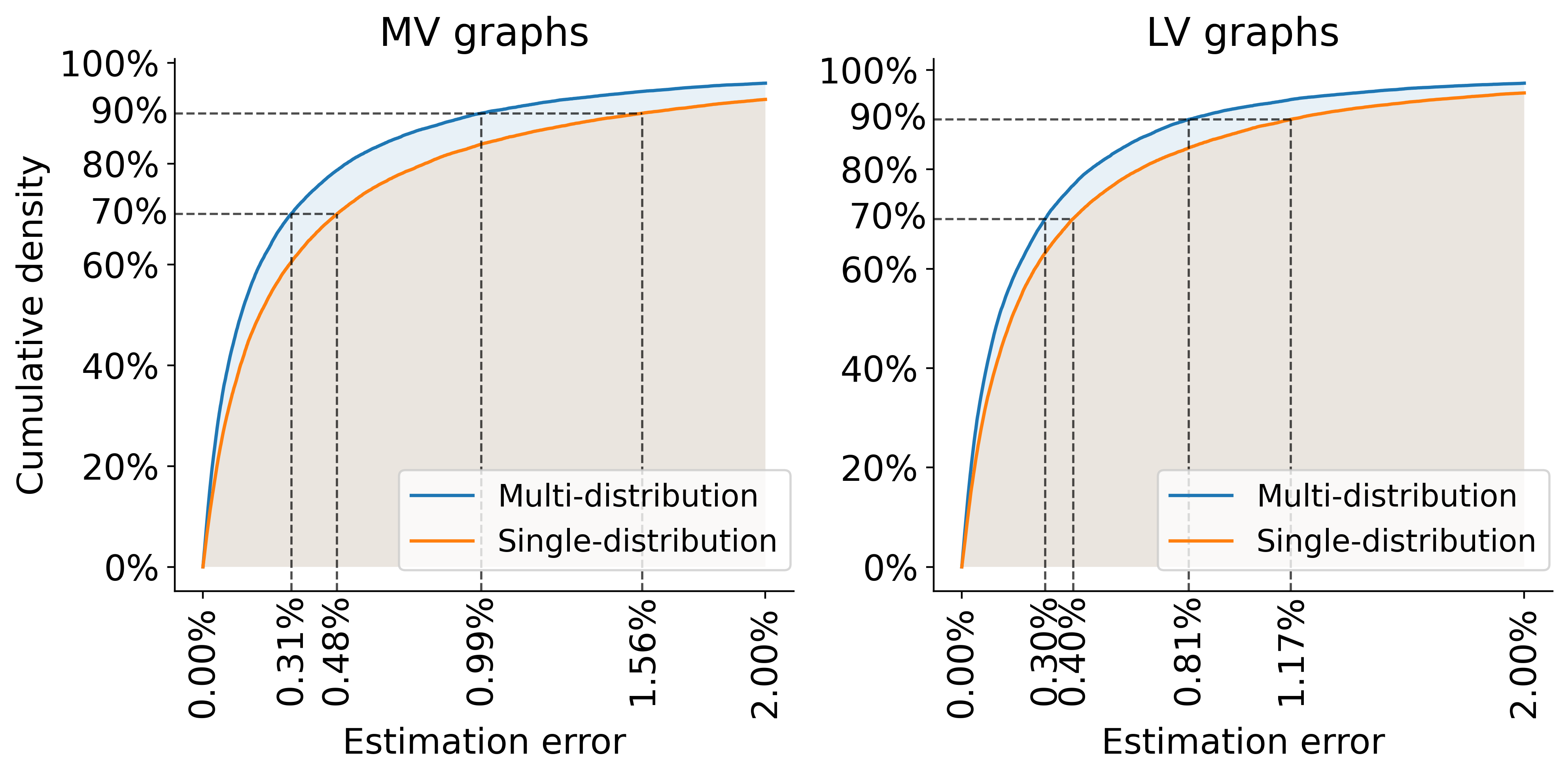
Figure 2: The cumulative density of approximation errors for the Wasserstein distance is shown for MV (left) and LV (right) graphs. Dashed lines indicate the 70th and 90th percentiles of the errors within each cumulative distribution.

We report the approximation errors for the initial and multiple distribution approximations, referred to as single-distribution and multi-distribution approximations, respectively. The single-distribution approximation corresponds to Step 1 of the method presented in Section 2.1.3, while the multi-distribution approximation corresponds to Step 2, i.e., the distances $\boldsymbol{D}_{1}$ and $\hat{\boldsymbol{D}}$. The results for the multi-distribution approximation are reported for the value of $\beta$ in Eqs. (6a)-(6b) that yields the smallest average error, which is $-0.5$ for both the MV and LV datasets.

Fig. 2 shows the cumulative density of the errors. The multi-distribution approximation outperforms the single-distribution approximation for both LV and MV graphs, with the difference becoming more pronounced for larger estimation errors. Furthermore, the multi-distribution yields average errors of 0.435% for the MV dataset and 0.380% for the LV dataset, while the single-distribution results in average errors of 0.640% and 0.489%, respectively.

Table 2: Wasserstein computation time in seconds.

	Single distribution	Additional distributions
MV	2	31
LV	122	1417

The multi-distribution approximation requires the computation of the set of 25 reference distributions, i.e., one initial and 24 references (see Section 2.1.3). The computation of the additional references is parallelized. The wall-clock times for the single distribution and additional distributions computations for the datasets are reported in Table 2. The additional reference distributions contain varying numbers of support vectors, with distributions having more support vectors resulting in longer execution times (see Sec. 2.1.1). Consequently, the time required for computing the single and additional distributions differs. Nevertheless, the total time needed for the multi-distribution approximation remains small, 33 seconds for the MV dataset and 1539 for the LV dataset (the sum of each row in Table 2). This demonstrates that the approximation quality of the single-distribution can be further refined with additional distributions while maintaining a low computational burden.

4.2 Clustering execution and validity indices

Table 3: Clustering execution time in seconds.

	Min.	Std.	Avg.	Max.
MV	5	0	5	7
LV	242	6	253	274

The execution time statistics for the clustering processes are reported in Table 3. These statistics correspond to the 50 kernel parameter initializations and the 50 Bayesian optimization iterations (see Section 3.1.4). The reported execution time includes the time taken to obtain the feature maps through kernel PCA and to perform k-medoids clustering on these maps. On average, the process takes 5 seconds for the MV graphs and 253 seconds for the LV graphs. Additionally, the standard deviations and the difference between the maximum and minimum times are minor. The clustering execution proves to be efficient, and the time scales linearly with respect to the number of graphs clustered. It is important to note that the execution time is independent of the graph sizes.

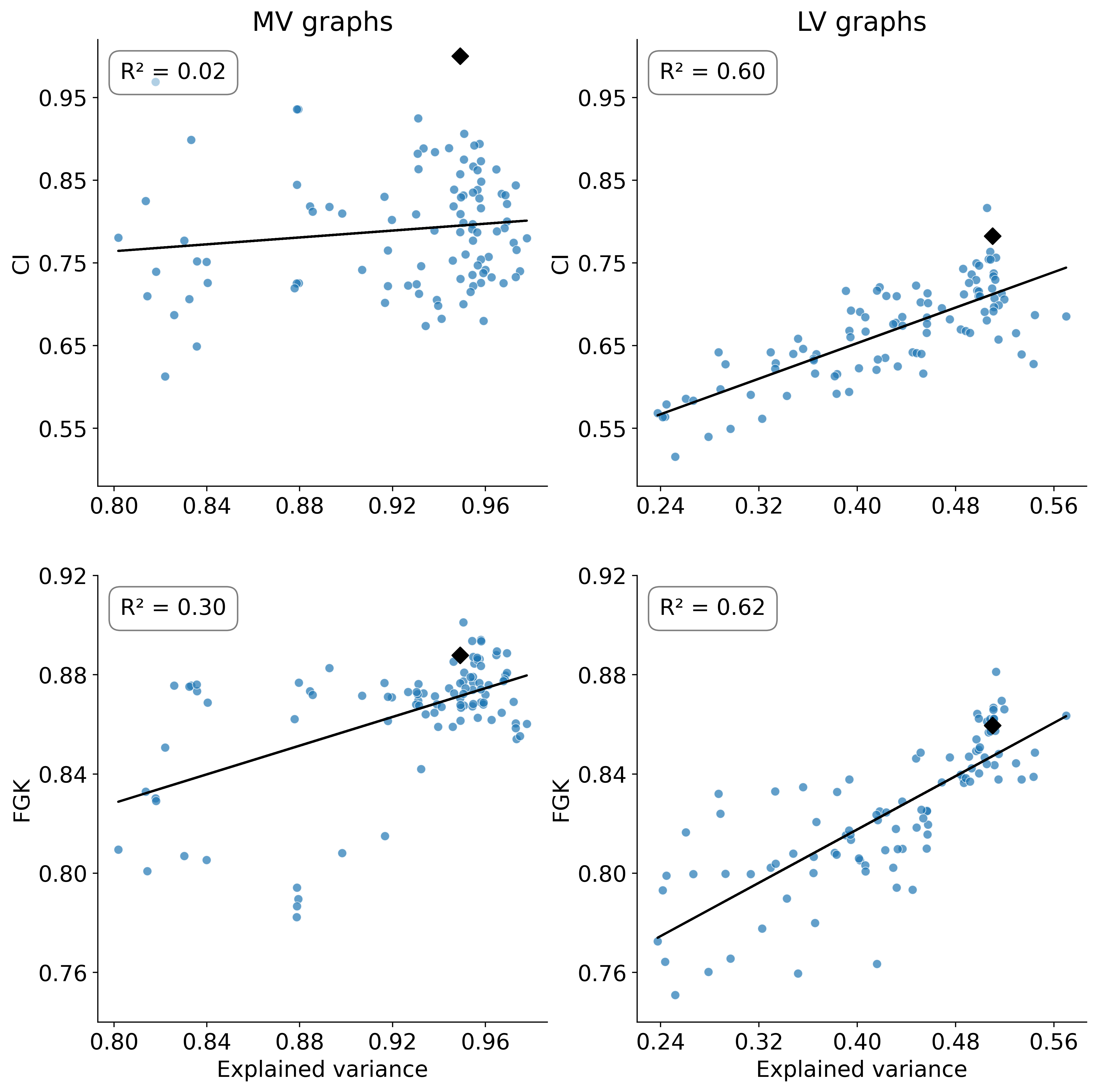
Figure 3: Validity indices plotted against the explained variance of the first five components. The validity indices corresponding to the selected clustering results are indicated with black diamonds.

Next, we analyze the relationship between the explained variance of the feature maps and the validity indices. Figure 3 reports the validity indices CI and FGK plotted against the explained variance of the first five components of the kernel PCA. For the MV graphs dataset, the CI shows no clear relationship with the explained variance. However, a subtle linear trend is observed between the FGK and the variance. On the other hand, the LV graphs dataset displays a linear relationship between CI/FGK values and the variance. Additionally, MV graphs generally exhibit higher CI and FGK values than the LV graphs. This difference can be attributed to the fact that the LV dataset requires more principal components than the MV dataset to explain the same variance. Furthermore, the difference in CI values is influenced by the k-medoids PAM method being more stable (used for the MV graphs) than the faster alternate method (used for the LV graphs).

4.3 Model selection and evaluation

Table 4: Normalized DB indices of MV graphs clustering.

	WK	PN	WP	WV
Voltage	0.227	0.796	1	0
Power	0.433	0.208	0	0.781
Power&Nodes	0.115	0	0.430	1
Average	0.258	0.335	0.477	0.594
Max	0.433	0.796	1	1

Table 5: Normalized DB indices of LV graphs clustering.

	CWK	PN	WP	WV
Voltage	0.232	0.826	1	0
Power	0.595	0.572	0	0.922
Power&Nodes	0	0	1	0.042
Average	0.277	0.466	0.667	0.321
Max	0.595	0.826	1	0.922

We sort the clustering solutions, corresponding to the 50 kernel parameter initializations and the 50 Bayesian optimization iterations, using the objective values obtained from Eq. (20). From the sorted solutions, we compute the context-dependent validity index in Eqs. (24a)-(24c) for the three solutions with the highest objective values. Afterward, the clustering solutions selected for the MV and LV cases are those that simultaneously yield the lowest average and maximum normalized DB scores (see Section 3.2.2). Table 4 and Table 5 report the normalized DB scores of the selected solutions for the MV and LV graphs, respectively. The MV clustering has an FGK value of 0.888 and a CI of 1, while the LV clustering has an FGK of 0.860 and a CI of 0.782 (indicated by the black diamonds in Figure 3). Furthermore, the WK method achieves the lowest average and maximum indices for both datasets compared to the other methods. Thus, the WK effectively incorporates the information of the nodal voltage distribution, the nodal power distribution, the graph’s total power demand, and the number of nodes.

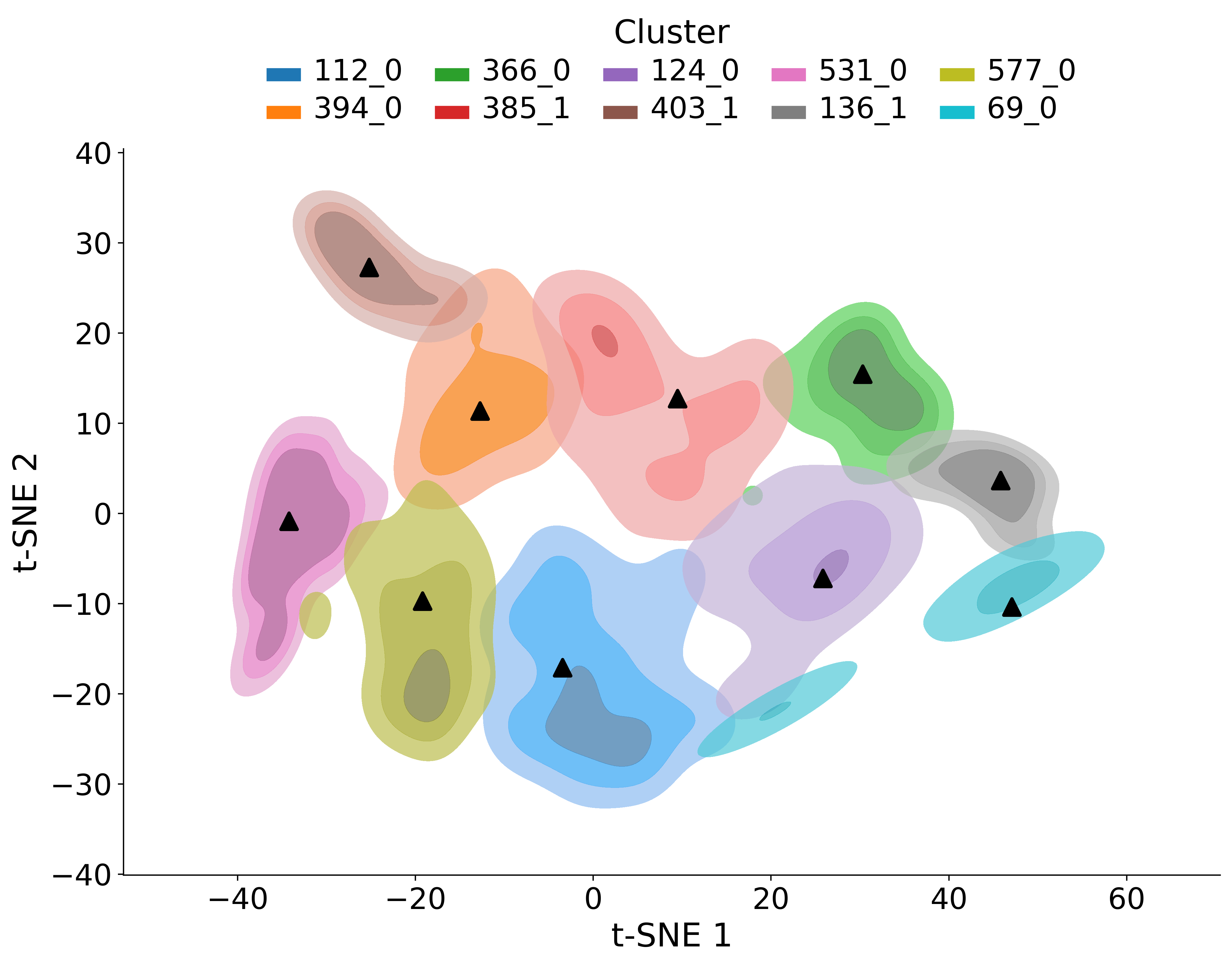
Figure 4: Projection via t-SNE of the MV graphs feature maps. The cluster medoids are indicated with a black triangle. The clusters are named after the identifier of the medoid in the dataset.

Figure 5: Projection via t-SNE of the LV graphs feature maps. The cluster medoids are indicated with a black triangle. The clusters are named after the identifier of the medoid in the dataset.

Figures 4 and 5 display the clusters for the MV and LV datasets, respectively. For visualization, we use a t-SNE projection, which is well-suited for high-dimensional data [46]. Specifically, the MV feature maps have 14 dimensions, while the LV feature maps have 222 dimensions, both of which are projected into two dimensions for visual inspection. Figures 4 and 5 show density plots with contour levels are shown, corresponding to kernel density estimations over the projected points, drawn with a threshold of 80% of the probability mass. Three different color levels represent areas of equal probability mass for each cluster. Additionally, the medoids are indicated with black triangles. The clusters are labeled according to the name of their medoids in the corresponding datasets.

We observe that the clusters show only slight overlaps and are well-distributed in the projected spaces. Although these visualizations are lower-dimensional projections, they confirm that the clusters are compact and exhibit clear separation. This outcome is expected given the high FGK values, which allow us to identify good quality clustering shapes in high dimensions. Moreover, the medoids tend to lie close to or within the contour level of the highest density in both figures. This result indicates that the medoids display central characteristics of their respective clusters, making them appropriate as representative prototypes.

Figure 6: Distributions of MV graphs by cluster, including mean nodal demand, mean nodal voltage, total demand, and the number of nodes. The medoids of each cluster are marked with black triangles.

Figure 7: Distributions of LV graphs by cluster, including mean nodal demand, mean nodal voltage, total demand, and the number of nodes. The medoids of each cluster are marked with black triangles.

We further examine the clusters with respect to 1) the mean nodal demand, 2) the mean nodal voltage, 3) the total demand, and 4) the number of nodes. Figures 6 and 7 show these properties for the MV and LV graphs, respectively, using the same colors as in Figures 4 and 5. We observe that most of the medoids, indicated by black triangles, lie within the interquartile ranges and close to the medians, which is expected if the medoids are representative objects of their clusters. Moreover, we found that the t-SNE axis 2 in Fig. 4 is related to the total demand and number of nodes in the MV graphs. Higher values on this axis correspond to lower total demand and fewer nodes, as observed in Fig. 6. Fig. 4 shows that for the t-SNE axis 1, the higher values correspond to lower nodal voltage means, similarly as in Fig. 6. For the LV graphs, we draw similar insights. The t-SNE axis 2 of Fig. 5 is related to the total demand of the graphs since higher values on this axis correspond to higher total demand (shown in Fig. 7). For the t-SNE axis 1, we observe that higher values are related to higher nodal voltage means.

5 Discussion

Section 4 provides insights into the application of the proposed framework in a real-world case study of PDGs. The results and their limitations shed light on avenues for future research. Firstly, we approximate Wasserstein distances with multiple references. The empirical evidence shows improved results compared to single reference approximation while being computationally tractable. Still, the convergence to the exact Wasserstein distances is not clearly understood. An exception is the trivial case when every distribution is used as a reference, in which the approximation becomes exact.

Secondly, the discrete distributions in the case study contain a number of support vectors on the order of $10^{2}$ (see Table 1), for which computing the exact distances with the references is manageable. However, the time required to solve this problem increases significantly with the number of support vectors. In some applications, an approximation of the discrete distributions may be needed, such as a particle approximation [9].

Lastly, we use the Kaiser criterion to choose the number of components in kernel PCA, which is a simple rule for denoising and dimensionality reduction. Nevertheless, it might be valuable to investigate the impact of component selection on clustering results and determine if there is an optimal number of components to retain. Since the explained variance affects the validity indices, as shown in Section 4.2, optimizing component selection could further improve the results.

6 Conclusions

In this article, we developed a clustering framework that leverages Wasserstein-based kernels, capable of simultaneously handling distributional and vectorial dissimilarity measures. The Wasserstein distances are approximated using multiple reference distributions through a linear optimal transport approach. Wasserstein-based kernels are then defined, using the approximated distances as input. Furthermore, to mitigate the impact of low-variance components in the clustering process, we employ kernel PCA. The quality of the clustering assignments is assessed using suitable validity indices. The potential of our framework is demonstrated in a case study involving 879 medium-voltage and 34,920 low-voltage power distribution graphs.

The results highlight the strengths of the proposed clustering framework. We show that the utilization of multiple distributions for pairwise distance approximation reduces estimation errors compared to a single distribution while maintaining low computational costs. The kernel PCA and k-medoids clustering process proved to be time-efficient and scalable. As confirmed by low-dimensional projections, the developed FGK index also efficiently detects well-separated and compact clusters. The Wasserstein-based kernel clustering method achieves the best performance according to the adopted context-dependent index. Furthermore, analysis of the cluster medoids confirms their representativeness as prototypes because they closely align with the medians of cluster properties. Moreover, the framework is not limited to handling graph-type data with discrete distributions and global properties vector representations. It can also be utilized for other data with these representations, such as images and point clouds, opening avenues for further research.

References

- Wang and Mi [2024] H. Wang, J. Mi, Intuitive-k-prototypes: A mixed data clustering algorithm with intuitionistic distribution centroid, Pattern Recognition (2024) 111062. doi:10.1016/j.patcog.2024.111062.
- Del Barrio et al. [2019] E. Del Barrio, J. A. Cuesta-Albertos, C. Matrán, A. Mayo-Íscar, Robust clustering tools based on optimal transportation, Statistics and Computing 29 (2019) 139–160.
- Lloyd [1982] S. Lloyd, Least squares quantization in PCM, IEEE transactions on information theory 28 (1982) 129–137.
- Rdusseeun and Kaufman [1987] L. Rdusseeun, P. Kaufman, Clustering by means of medoids, in: Proceedings of the statistical data analysis based on the L1 norm conference, Neuchatel, switzerland, volume 31, 1987.
- Ye et al. [2024] Z. Ye, L. Yao, Y. Zhang, S. Gustin, Self-supervised cross-modal visual retrieval from brain activities, Pattern Recognition 145 (2024) 109915. doi:10.1016/j.patcog.2023.109915.
- Jayasumana et al. [2015] S. Jayasumana, R. Hartley, M. Salzmann, H. Li, M. Harandi, Kernel methods on Riemannian manifolds with Gaussian RBF kernels, IEEE transactions on pattern analysis and machine intelligence 37 (2015) 2464–2477.
- Lee et al. [2015] H. Lee, H.-J. Ahn, K.-R. Kim, P. T. Kim, J.-Y. Koo, Geodesic clustering for covariance matrices, Communications for Statistical Applications and Methods 22 (2015) 321–331.
- Zhang et al. [2022] S. Zhang, Y. Wang, Y. Zhang, P. Wan, J. Zhuang, Riemannian Distance-Based Fast K-Medoids Clustering Algorithm for Cooperative Spectrum Sensing, IEEE Systems Journal 16 (2022) 880–890. doi:10.1109/JSYST.2021.3056547.
- Wang et al. [2013] W. Wang, D. Slepčev, S. Basu, J. A. Ozolek, G. K. Rohde, A linear optimal transportation framework for quantifying and visualizing variations in sets of images, International journal of computer vision 101 (2013) 254–269.
- Togninalli et al. [2019] M. Togninalli, E. Ghisu, F. Llinares-López, B. Rieck, K. Borgwardt, Wasserstein weisfeiler-lehman graph kernels, Advances in neural information processing systems 32 (2019).
- Li and Wang [2008] J. Li, J. Z. Wang, Real-Time Computerized Annotation of Pictures, IEEE Transactions on Pattern Analysis and Machine Intelligence 30 (2008) 985–1002. doi:10.1109/TPAMI.2007.70847.
- Ye et al. [2017] J. Ye, P. Wu, J. Z. Wang, J. Li, Fast discrete distribution clustering using Wasserstein barycenter with sparse support, IEEE Transactions on Signal Processing 65 (2017) 2317–2332.
- Verdinelli and Wasserman [2019] I. Verdinelli, L. Wasserman, Hybrid Wasserstein distance and fast distribution clustering, Electronic Journal of Statistics 13 (2019) 5088 – 5119. doi:10.1214/19-EJS1639.
- i Garcia et al. [2023] V. G. i Garcia, X. Gual-Arnau, M. V. Ibáñez, A. Simó, A gaussian kernel for kendall’s space of m-d shapes, Pattern Recognition 144 (2023) 109887. doi:10.1016/j.patcog.2023.109887.
- Alavi and Hashemi [2022] F. Alavi, S. Hashemi, A bi-level formulation for multiple kernel learning via self-paced training, Pattern Recognition 129 (2022) 108770.
- Rahimzadeh Arashloo [2024] S. Rahimzadeh Arashloo, Large-margin multiple kernel lp-svdd using frank–wolfe algorithm for novelty detection, Pattern Recognition 148 (2024) 110189. doi:10.1016/j.patcog.2023.110189.
- Hofmann et al. [2008] T. Hofmann, B. Schölkopf, A. J. Smola, Kernel methods in machine learning, The Annals of Statistics 36 (2008) 1171 – 1220. doi:10.1214/009053607000000677.
- Titouan et al. [2019] V. Titouan, N. Courty, R. Tavenard, R. Flamary, Optimal transport for structured data with application on graphs, in: International Conference on Machine Learning, PMLR, 2019, pp. 6275–6284.
- Wiroonsri [2024] N. Wiroonsri, Clustering performance analysis using a new correlation-based cluster validity index, Pattern Recognition 145 (2024) 109910. doi:10.1016/j.patcog.2023.109910.
- Arbelaitz et al. [2013] O. Arbelaitz, I. Gurrutxaga, J. Muguerza, J. M. Pérez, I. Perona, An extensive comparative study of cluster validity indices, Pattern Recognition 46 (2013) 243–256. doi:10.1016/j.patcog.2012.07.021.
- Davies and Bouldin [1979] D. L. Davies, D. W. Bouldin, A Cluster Separation Measure, IEEE Transactions on Pattern Analysis and Machine Intelligence PAMI-1 (1979) 224–227. doi:10.1109/TPAMI.1979.4766909.
- Vinh et al. [2010] N. X. Vinh, J. Epps, J. Bailey, Information Theoretic Measures for Clusterings Comparison: Variants, Properties, Normalization and Correction for Chance, Journal of Machine Learning Research 11 (2010) 2837–2854. URL: http://jmlr.org/papers/v11/vinh10a.html.
- Su et al. [2024] R. Su, Y. Guo, C. Wu, Q. Jin, T. Zeng, Kernel correlation–dissimilarity for multiple kernel k-means clustering, Pattern Recognition 150 (2024) 110307. doi:10.1016/j.patcog.2024.110307.
- Alam et al. [2024] A. Alam, A. Malhotra, I. D. Schizas, Online kernel-based clustering, Pattern Recognition (2024) 111009.
- Tomašev and Radovanović [2016] N. Tomašev, M. Radovanović, Clustering evaluation in high-dimensional data, in: Unsupervised learning algorithms, Springer, 2016, pp. 71–107.
- Kolouri et al. [2021] S. Kolouri, N. Naderializadeh, G. K. Rohde, H. Hoffmann, Wasserstein Embedding for Graph Learning, 2021. arXiv:2006.09430.
- Goodman and Kruskal [1949] L. Goodman, W. Kruskal, Measures of associations for cross-validations, J. Am. Stat. Assoc 49 (1949) 732–764.
- Villani et al. [2009] C. Villani, et al., Optimal transport: old and new, volume 338, Springer, 2009.
- Crook et al. [2024] O. M. Crook, M. Cucuringu, T. Hurst, C.-B. Schönlieb, M. Thorpe, K. C. Zygalakis, A linear transportation lp distance for pattern recognition, Pattern Recognition 147 (2024) 110080.
- Cuturi [2013] M. Cuturi, Sinkhorn Distances: Lightspeed Computation of Optimal Transport, in: C. Burges, L. Bottou, M. Welling, Z. Ghahramani, K. Weinberger (Eds.), Advances in Neural Information Processing Systems, volume 26, Curran Associates, Inc., 2013. URL: https://proceedings.neurips.cc/paper_files/paper/2013/file/af21d0c97db2e27e13572cbf59eb343d-Paper.pdf.
- De Plaen et al. [2020] H. De Plaen, M. Fanuel, J. A. Suykens, Wasserstein exponential kernels, in: 2020 International Joint Conference on Neural Networks (IJCNN), IEEE, 2020, pp. 1–6.
- Ren et al. [2022] J. Ren, K. Hua, Y. Cao, Global optimal k-medoids clustering of one million samples, Advances in Neural Information Processing Systems 35 (2022) 982–994.
- Zhang et al. [2024] C. Zhang, K. Gai, S. Zhang, Matrix normal pca for interpretable dimension reduction and graphical noise modeling, Pattern Recognition 154 (2024) 110591. doi:10.1016/j.patcog.2024.110591.
- Jolliffe and Cadima [2016] I. T. Jolliffe, J. Cadima, Principal component analysis: a review and recent developments, Philosophical transactions of the royal society A: Mathematical, Physical and Engineering Sciences 374 (2016) 20150202.
- Kaiser [1960] H. F. Kaiser, The application of electronic computers to factor analysis, Educational and psychological measurement 20 (1960) 141–151.
- Sterge et al. [2020] N. Sterge, B. Sriperumbudur, L. Rosasco, A. Rudi, Gain with no pain: Efficiency of kernel-pca by nyström sampling, in: International Conference on Artificial Intelligence and Statistics, PMLR, 2020, pp. 3642–3652.
- Guo and Wu [2024] Y. Guo, G. Wu, A restarted large-scale spectral clustering with self-guiding and block diagonal representation, Pattern Recognition 156 (2024) 110746. doi:10.1016/j.patcog.2024.110746.
- He and Zhang [2018] L. He, H. Zhang, Kernel K-means sampling for Nyström approximation, IEEE Transactions on Image Processing 27 (2018) 2108–2120.
- Merrill and Olson [2020] N. Merrill, C. C. Olson, Unsupervised ensemble-kernel principal component analysis for hyperspectral anomaly detection, in: Proceedings of the IEEE/CVF conference on computer vision and pattern recognition workshops, 2020, pp. 112–113.
- Nogueira [14 ] F. Nogueira, Bayesian Optimization: Open source constrained global optimization tool for Python, 2014–. URL: https://github.com/fmfn/BayesianOptimization.
- Oneto et al. [2025] A. Oneto, B. Gjorgiev, F. Tettamanti, G. Sansavini, Large-scale generation of geo-referenced power distribution grids from open data with load clustering, Sustainable Energy, Grids and Networks (2025) 101678. doi:https://doi.org/10.1016/j.segan.2025.101678.
- Flamary et al. [2021] R. Flamary, N. Courty, A. Gramfort, M. Z. Alaya, A. Boisbunon, S. Chambon, L. Chapel, A. Corenflos, K. Fatras, N. Fournier, L. Gautheron, N. T. Gayraud, H. Janati, A. Rakotomamonjy, I. Redko, A. Rolet, A. Schutz, V. Seguy, D. J. Sutherland, R. Tavenard, A. Tong, T. Vayer, POT: Python Optimal Transport, Journal of Machine Learning Research 22 (2021) 1–8. URL: http://jmlr.org/papers/v22/20-451.html.
- Aridas et al. [23 ] C. Aridas, J.-O. Joswig, T. Mathieu, R. Yurchak, scikit-learn-extra: A set of useful tools compatible with scikit-learn, 2023–. URL: https://github.com/scikit-learn-contrib/scikit-learn-extra.
- Leonard Kaufman [1990] P. J. R. Leonard Kaufman, Partitioning Around Medoids (Program PAM), John Wiley & Sons, Ltd, 1990, pp. 68–125. doi:10.1002/9780470316801.ch2.
- Park and Jun [2009] H.-S. Park, C.-H. Jun, A simple and fast algorithm for K-medoids clustering, Expert Systems with Applications 36 (2009) 3336–3341. doi:10.1016/j.eswa.2008.01.039.
- Van der Maaten and Hinton [2008] L. Van der Maaten, G. Hinton, Visualizing data using t-SNE., Journal of machine learning research 9 (2008).