End-to-End Optimal Detector Design with Mutual Information Surrogates

Abstract

We introduce a novel approach for end-to-end black-box optimization of high energy physics (HEP) detectors using local deep learning (DL) surrogates. These surrogates approximate a scalar objective function that encapsulates the complex interplay of particle-matter interactions and physics analysis goals. In addition to a standard reconstruction-based metric commonly used in the field, we investigate the information-theoretic metric of mutual information. Unlike traditional methods, mutual information is inherently task-agnostic, offering a broader optimization paradigm that is less constrained by predefined targets.

We demonstrate the effectiveness of our method in a realistic physics analysis scenario: optimizing the thicknesses of calorimeter detector layers based on simulated particle interactions. The surrogate model learns to approximate objective gradients, enabling efficient optimization with respect to energy resolution.

Our findings reveal three key insights: (1) end-to-end black-box optimization using local surrogates is a practical and compelling approach for detector design, providing direct optimization of detector parameters in alignment with physics analysis goals; (2) mutual information-based optimization yields design choices that closely match those from state-of-the-art physics-informed methods, indicating that these approaches operate near optimality and reinforcing their reliability in HEP detector design; and (3) information-theoretic methods provide a powerful, generalizable framework for optimizing scientific instruments. By reframing the optimization process through an information-theoretic lens rather than domain-specific heuristics, mutual information enables the exploration of new avenues for discovery beyond conventional approaches.

I Introduction

Problem Definition
$\theta\in\mathbb{R}^{F}$	Design parameter vector for a detector characterized by $F$ features
$D_{\theta}$	Simulated detector parametrized by $\theta$
$x\in\mathbb{R}^{U}$	Particle with $U$ truth features
$y\in\mathbb{R}^{V}$	$V$-dimensional detector response for particle $x$
$\delta\to\mathbb{R}$	Scalar valued objective function
$R$	Objective model implementing $\delta$
$S$	Surrogate model approximating $\delta$
Iterative Optimization
$\theta^{k}\in\mathbb{R}^{F}$	One of $K$ test points in the local neighborhood of $\theta$
$x^{k}\in\mathbb{R}^{M\times U}$	$M$ particles generated for test point $k$
$y^{k}\in\mathbb{R}^{M\times V}$	Response of a detector parametrized by $\theta^{k}$ to particles $x^{k}$

Table 1: Summary of symbols and their definitions.

The rapid progress of scientific research, driven by growing datasets and increasingly sophisticated analysis methods, places substantial demands on detector development in HEP. As experiments become more complex, determining optimal detector design parameters becomes increasingly challenging. Notable examples include the forthcoming high-luminosity upgrade of the CERN Large Hadron Collider (LHC) [1], where the number of collisions per bunch crossing is expected to increase by an order of magnitude, as well as the conceptual design of the Future Circular Collider (FCC) [2], which aims to achieve significantly higher precision in the FCC-ee phase and significantly higher center-of-mass energies, reaching up to $100\text{\,}\mathrm{TeV}$ in the FCC-hh phase – far exceeding the $14\text{\,}\mathrm{TeV}$ of the LHC—along with enhanced luminosities for precision measurements and new physics searches. Both phases will pose significant and new challenges to the design of large-scale detectors.

Detector optimization is inherently challenging. The design parameter space is typically high-dimensional, requiring sophisticated simulation software to model detector response accurately. Moreover, the entire optimization process is stochastic, adding an additional layer of complexity.

Furthermore, the evaluation of the fitness of a set of parameters presents two major challenges. First, it incorporates detector simulations that are typically non-differentiable, or at the very least, the gradient with respect to the design parameters is not readily accessible. Second, the parameter space may exhibit multiple local and global optima that are unknown a priori. Given the high computational cost of evaluating the simulation, it is impractical to sample the design space densely enough to fully characterize its structure [3].

To address these challenges, we propose an iterative machine learning (ML)-based optimization framework for determining the optimal design parameters of a simulated HEP detector. This approach enables end-to-end optimization by leveraging a differentiable DL surrogate.

Problem Statement

End-to-end detector development in HEP typically involves a forward simulation and backward reconstruction step (see Table 1 for a summary of symbol definitions). Given a set of design parameters $\theta$ (e.g., number and thickness of detector segments) and an objective metric $\delta$ (e.g. energy resolution), a forward simulation is constructed to model the interaction of a physics process $X$ (e.g., photon production) with the detector $D_{\theta}$. This simulation captures the resulting signals, such as energy deposits in calorimeter cells. The detector response to the physics process, $D_{\theta}(X)$, is then processed by a reconstruction module, which aims to recover the original event $\hat{X}$ from these recorded traces. The primary goal of this process is to minimize the discrepancy between the true event $X$ and its reconstructed counterpart $\hat{X}$ under the chosen metric $\delta$ with respect to the optimal configuration $D_{\theta^{*}}$:

$$\theta^{*}=\operatorname*{arg\,min}_{\theta}\delta(X,D_{\theta}(X)).$$

In the standard setup, the objective function involves a Monte Carlo simulator and is not uniquely defined, rendering the optimization problem non-differentiable with respect to $\theta$. Consequently, heuristic methods are typically employed to navigate the design space.
In this work, we introduce a surrogate model trained to approximate a localized region of the design parameter space $\theta$ and performance metric $\delta$. By enabling differentiation with respect to the design parameters, this surrogate model facilitates an efficient search for the optimal detector configuration $D_{\theta^{*}}$.

Contribution

We implement an end-to-end optimization framework that integrates the forward detector response and backward reconstruction process into a unified objective.
Our innovation is twofold. First, we define the optimization objective as a scalar-valued function, enabling efficient iterative optimization while encapsulating the local optimality of the detector design for a given physics task within a single metric. Locality, in this context, refers to surrogate models operating within a confined region of the parameter space at each iteration, a necessary strategy given the impracticality of exhaustively sampling the entire space in realistic detector optimization. Second, we introduce and systematically study Transfer Learning (TL) to mitigate the limitations of locality. We test the hypothesis that the surrogate model can transfer knowledge about the local optimality across iterations, progressively refining and expanding the explored regions of the design parameter landscape.

Designing an effective objective function is a central challenge in experimental optimization within the fundamental sciences [4]. In this work, we introduce two optimization framework variants, distinguished primarily by their choice of objective function. A key aspect of this study is the comparison between these two fundamentally different metrics.
The first variant, RECO-OPT, follows a conventional approach commonly used in high-energy physics (HEP) detector development. Here, the objective function is defined as the reconstruction loss, which quantifies the discrepancy between a particle’s true features and their approximations obtained through a detector reconstruction model. This serves as a benchmark for evaluating optimization performance, aligning with established methodologies.
In contrast, the second variant, MI-OPT, adopts an information-theoretic perspective, abstracting the optimization process from predefined target specifications. Instead of relying on explicit objectives, MI-OPT optimizes mutual information between a particle’s true features and the detector’s output signal. This task-agnostic metric eliminates the need for user-defined objectives, providing a more generalizable approach to instrument optimization.
Additionally, both frameworks can incorporate constraints to accommodate practical considerations, such as material limitations or financial restrictions.

In Section II we discuss related work, in Section III we present the data of our studies, in Section IV we detail the developed methods. The experimental procedures are outlined in Section V while the results are presented in Section VI. The conclusion and outlook for further research is given in Section VII.

II Related Work

In general, optimizing a non-differentiable system can be approached in three ways: transforming it into a differentiable form, applying gradient-free optimization methods, or constructing a surrogate model to approximate the system.

One approach to making a non-differentiable system differentiable is to leverage tools from DL, in particular automatic differentiation (AD) techniques which allow for precise gradient computation. Recent studies in HEP have augmented existing forward (e.g. Geant4 simulation, particle showering simulation) and backward (e.g. jet-clustering) toolkits by algorithmic differentiation [5, 6, 7, 8]. Others have utilized these advancements to develop fully differentiable pipelines for end-to-end optimization of detector configurations, demonstrating significant performance gains and highlighting the potential of DL-driven optimization in future HEP experiments [9, 10, 11]. However, these methods require rewriting the detector simulation into a differentiable variant, which can be a significant limitation. Our approach aims to achieve the same end-to-end optimization while circumventing the need for such modifications.

There are also optimization techniques that operate without requiring gradient information of the objective function. Examples include Reinforcement Learning (RL) [12, 13] and genetic algorithms [14, 15, 16, 17]. A drawback of RL is its high demand for data and computational resources. While genetic algorithms are more lightweight, they often face convergence challenges, in particular for a large number of parameters. Both heuristics demand a substantial number of objective function evaluations. This becomes problematic in HEP detector design, where each evaluation is computationally expensive.

Bayesian Optimization (BO) is another gradient-free technique that has gained prominence in scenarios where quantifying the uncertainty of objective function predictions is essential. This approach leverages Gaussian Process (GP) models, which enable non-parametric global optimization across diverse domains (for an overview, see [18]). While traditionally employed for global optimization, recent advancements have introduced localized variants [19, 20, 21], addressing key limitations such as scalability to high-dimensional problems—making them more suitable for applications like the one considered here. However, several limitations persist. The computational cost of BO scales as $\mathcal{O}(N^{2})$ or $\mathcal{O}(N^{3})$ with the number of samples, posing challenges for HEP applications where large datasets are common. Moreover, BO requires problem-specific tuning, including the selection of handcrafted kernels and hyperparameters, which assumes prior knowledge of the underlying objective function or response structure [22, 23, 24]. Given the complexity of our objective space and the need for a flexible framework capable of seamlessly integrating new objectives (e.g., the identification of particle types), we instead opt for a DL surrogate approach.

Recently, the use of DL-driven surrogates for black-box optimization tasks has gained significant traction [25, 26, 27]. The choice of the surrogate model depends on the nature and domain of the problem. Notably, generative approaches have shown success in various applications (for an overview, see [28]). For example, [29] tackles detector optimization in HEP with intractable likelihoods using local generative surrogates. By iteratively exploring the design space, the surrogate approximates the objective function’s gradient, guiding optimization toward an optimal design. This approach is extended by [30] to an end-to-end framework, integrating forward simulation and backward reconstruction while reducing surrogate complexity. Building on these advancements, we propose an end-to-end optimization framework that leverages a novel information-theoretic methodology.

The choice of optimization metric plays a crucial role in most related studies. Information-theoretic metrics have proven effective across various domains and have been, for example, incorporated into BO frameworks discussed earlier [31, 32].

A well-established information-theoretic measure for capturing nonlinear statistical dependencies is the mutual information criterion [33, 34]. This metric has been successfully applied in diverse fields, including biology [35], neuroscience [36], speech recognition [37], and linguistics [38], demonstrating its versatility and effectiveness. Given these strengths, we adopt mutual information as the primary metric for our investigation and compare its performance to classic approaches discussed above, demonstrating how the new measure opens the avenue for a task-agnostic instrument assessment.

III Data

In this work, we employ a dataset generated by simulating single photons incident on a calorimeter detector. These simulations are carried out using the Geant4 framework [39, 40, 41], specifically employing the FTFP_BERT physics list. The detector consists of multiple layers, each comprising two distinct material segments: a lead absorber and a lead-tungstate scintillator, as depicted schematically in Figure 1. For this proof of concept, we choose PbWO₄ as the active scintillator material, a commonly used scintillator material in HEP  [42, 43, 44], and Pb as the absorber. During simulation, only the energy deposited in the active material is recorded, and this information is passed on to subsequent processing steps. We do not include a detailed simulation of the readout electronics.

The thickness of each material segment is treated as an optimizable design parameter. Given a nominal parameter vector $\theta\in\mathbb{R}^{F}$ where $F$ is the number of design features (for example $F=6$ if we want to optimize the segment-thicknesses of a detector composed of three layers), we draw a collection of $K$ perturbed parameter vectors

$$\theta^{k}\sim\mathcal{N}(\theta,\sigma),$$

where the width $\sigma$ is chosen to be of the order of the radiation length (approximately 1 cm) [42]. This strategy follows a trust-region approach similar to that outlined in [29, 45]. For each parameter vector $\theta^{k}$, we simulate particles incident on the detector, generating true features $x^{k}$, as well as measured features $y^{k}$.

Our inputs, $x$, as well as their progression through the detector (e.g., particle showering) and its response, $y$, are inherently stochastic.

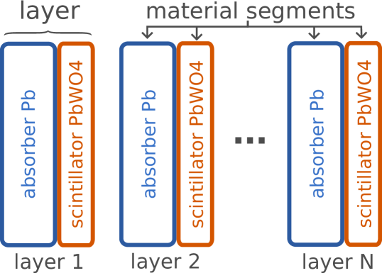
Figure 1: Calorimeter consisting of layers of interleaved lead absorber and lead-tungstate scintillator segments.

IV Methods & Models: Optimal Design Surrogate

The primary purpose of the optimization is to determine the optimal thicknesses for the scintillator and absorber segments of a multi-layer calorimeter (Figure 1). The design parameters $\theta$ in our study thus correspond to thickness values in centimeters.

We develop two local surrogate optimization pipelines that differ primarily in their choice of objective metric $\delta$ (see Section I) and type of surrogate model used. The first approach, RECO-OPT, relies on a conventional reconstruction accuracy metric commonly used in detector assessment as well as a generative surrogate. RECO-OPT serves as a reference baseline typically used in the field. The second approach, MI-OPT, introduces an innovative optimization framework based on the information-theoretic metric of mutual information. This novel perspective enhances task-agnostic optimization and is invariant under homeomorphic transformations [46], offering a more robust and generalizable solution.

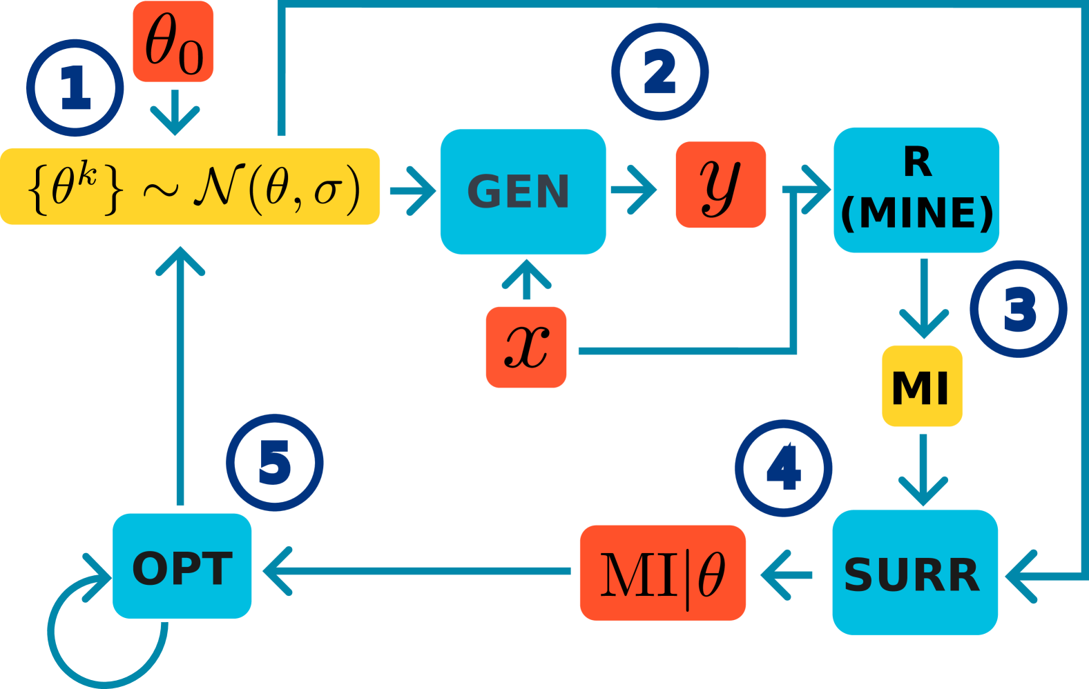
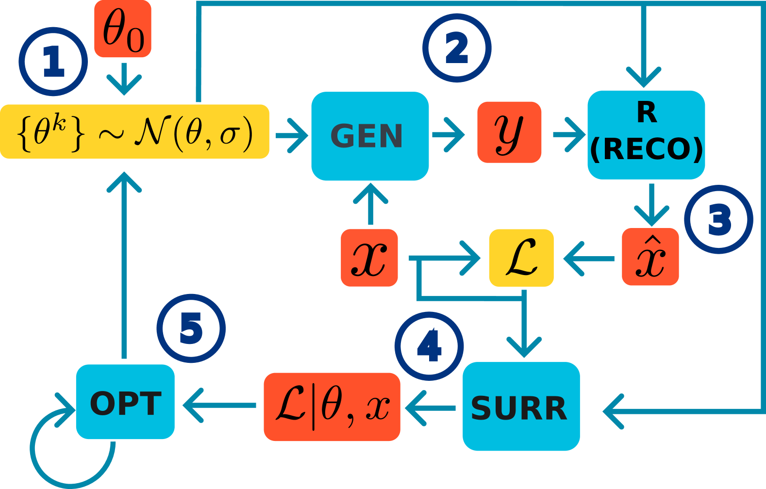
Figure 2: Two developed optimization pipelines: MI-OPT using mutual information as the objective function (left) and REC-OPT using the loss of a reconstruction model for that purpose (right).

Optimization loop

Both variants are integrated into an optimization loop framework which consists of five main parts:

1. Sampling of a set of test points from a local neighborhood in the design parameter space.

2. Simulation of a physics process and detector response (Geant4, see Section III).

3. Training of an objective model $R$ which computes the objective function $\delta$.

4. Training of a surrogate model $S$ to approximate the relationship between objective function $\delta$ and parameters $\theta$.

5. Gradient descent on the surrogate’s approximated objective with respect to the design parameters $\frac{\partial S}{\partial\theta}\approx\frac{\partial\delta}{\partial\theta}$.

The framework for both variants is illustrated in Figure 2 (MI-OPT on the left, RECO-OPT on the right) and described in detail below.

At the start of each optimization cycle, MI-OPT and RECO-OPT follow an identical procedure. Each iteration begins with an initial nominal parameter, $\theta$. Based on this nominal value, a set of test points is generated from its local neighborhood (Figure 2, step \raisebox{-.9pt} {1}⃝). Specifically, $K$ neighboring candidates, $\theta^{k}$ are sampled from a normal distribution centered at nominal $\theta$, with a standard deviation $\sigma$ that defines the neighborhood size: $\{\theta^{k}\}_{k=1}^{K}\sim\mathcal{N}(\theta,\sigma)$. The locality parameter $\sigma$ is set to $1.5\text{\,}\mathrm{cm}$.

For each parameter vector $\theta^{k}\in\mathbb{R}^{F}$, we simulate $M$ photons incident on the detector, generating $U$ true features per particle $x^{k}\in\mathbb{R}^{M\times U}$, as well as their corresponding $V$ measured calorimeter energy deposits $y^{k}\in\mathbb{R}^{M\times V}$ (Figure 2, step \raisebox{-.9pt} {2}⃝).

In each iteration of the pipeline, the triplets $\{\theta^{k},x^{k},y^{k}\}_{k=1}^{K}$ are used as inputs to the objective ML models. The objective model $R$ implements the objective criterion and computes a corresponding metric $\delta^{k}$ for each triplet (Figure 2, step \raisebox{-.9pt} {3}⃝). Based on the quadruplet $\{x^{k},y^{k},\theta^{k},\delta^{k}\}_{k=1}^{K}$, a surrogate model $S$ learns the relationship between the inputs and the target objective (Figure 2, step \raisebox{-1.0pt} {4}⃝). Parts \raisebox{-.9pt} {3}⃝ and \raisebox{-.9pt} {4}⃝ of the pipeline differ between MI-OPT and RECO-OPT in terms of objective models, surrogate models and objective function. These differences are discussed in detail in the dedicated paragraphs below.

After training the surrogate on $K$ new candidate points, stochastic gradient descent (SGD) is applied to identify the next optimal design parameters. By following the gradient $-\frac{\partial S}{\partial\theta}$, the optimizer searches for the most promising parameter set based on the learned approximation of the objective function. This search is confined to a local neighborhood around the current nominal $\theta$ and is halted if it exceeds predefined boundaries. Once a new optimal value is determined, the algorithm updates the nominal $\theta$ accordingly and proceeds to the next iteration. The process repeats from step \raisebox{-.9pt} {1}⃝, continuing until a set number of iterations is completed. The entire end-to-end optimization procedure is summarized in the framework Algorithm 1.

Algorithm 1 End-to-end Optimization Loop

1:number K of $\theta$ candidate points, number $M$ of particles $x$, size of the local region $\epsilon$, number of iterations I, measure of locality $d$

2:Choose initial nominal $\theta=\theta_{0}$

3:while $i\leq\text{I}$ do

4:  Sample $\mathbf{\theta}^{k}\sim\mathcal{N}(\mathbf{\theta},\sigma)$, $k=1,\ldots,K$

5:  For each $\mathbf{\theta}^{k}$, sample $M$ truth inputs $x^{k}\sim q(x)$

6:  Run detector simulation $y^{k}=D(x^{k},\theta^{k})$

7:  Obtain surrogate

8:   $\nabla_{\theta}S\leftarrow$ RECO-OPT($\{x^{k},y^{k},\theta^{k}\}$) or

9:   $\nabla_{\theta}S\leftarrow$ MI-OPT($\{x^{k},y^{k},\theta^{k}\}$)

10:  while $d(\theta^{*},\theta)<\epsilon$ do

11:   $\theta^{*}\leftarrow\text{SGD}(\theta,\nabla_{\theta}S)$

12:  end while

13:  $\theta\leftarrow\theta^{*}$

14:  $i=i+1$

15:end while

The next two subsections describe objective models and surrogates of RECO-OPT and MI-OPT in more detail.

RECO-OPT

For the standard, explicit reconstruction based optimization, the objective function is taken to be a normalized mean squared error loss between the true energy $x^{k}$ and some reconstructed energy. The objective model $R(y^{k}|\theta^{k})$ is trained to reconstruct the true energy $x^{k}$ of the incident photon from the energy deposited in the scintillators $y^{k}$. The model is implemented as a Multi-Layer Perceptron (MLP).

A generative surrogate model $S_{\omega}(z,x^{k},\theta^{k})$ is then trained to approximate the simulation and reconstruction step, directly predicting the loss of the reconstruction model $\delta^{k}$, for a given $\{x^{k},\theta^{k}\}$ pair.

Normalizing flows [47, 48, 49], one form of generative model that can be used as a surrogate, model the distribution $p_{w}$ of some data $\mathbf{w}$ as a bijective transformation $f$ from a known noise distribution $\mathbf{z}\sim p_{z}(z)$, and can be used for conditional distributions $p_{w}(\mathbf{w|c})$ [50].

Since the end-to-end approach maps to one output scalar, we introduce the one-dimensional normalizing flow (1D NF) model, which uses a piecewise linear transformation as our bijective function $f$. This is similar to the piecewise linear coupling transforms used in [51] except this is not structured as a coupling transform, given that our input is scalar valued.

A piecewise linear transform $f$ of an input $w$ is defined between some $w_{min}$ and $w_{max}$, where the interval between the two values is divided based on a preselected number of bins, $N_{bins}$. Values below $w_{min}$ are mapped to a constant value $\alpha$ while values above $w_{max}$ are mapped to the value of the highest bin. For a given input, an MLP that takes the conditional values $\mathbf{c}$ as input is used to predict the slopes $m_{i}$ in each linear piece. The output of the MLP is then used to parameterize the piecewise linear transformation and calculate the output $f(w)$ as:

$$f(w)=\begin{cases}\alpha&\text{if }w<w_{min}\\ m_{i}(w-w_{\text{offset}})+b_{i}&\text{if }w\in\text{bin}_{i}\end{cases}$$ (1)

where $m_{i}$ and $b_{i}$ are the slope and intercept of the linear transformation in the $i$-th bin, and $w_{\text{offset}}$ the lower bound of some given bin.

The 1D NF surrogate is trained to transform between a normal distribution $\mathcal{N}(0,1)$ and the logarithm of the distribution of the reconstruction loss, conditioned on the true energy $x$ and detector parameters $\mathbf{\theta}$. The logarithm of the reconstruction loss is chosen as it is close to a normal distribution. For evaluation, we consider the exponent of the surrogate output. The surrogate is trained by minimizing a negative log-likelihood loss. When the surrogate is trained, given an energy $x$, a set of detector parameters $\theta$, and some sampled $z$, the learned distribution of reconstruction losses for these conditional values can be sampled from, estimating the loss for a single event. These sample outputs are differentiable with respect to $\theta$ and can be used to optimize the surrogate parameters via gradient descent. A description of the procedure is given in surrogate Algorithm 2.

Algorithm 2 RECO-OPT Surrogate Variant

1:Surrogate generative model $S_{\omega}$

2:Train objective model $R_{\psi}(y|\theta)$

3:Fix weights $\psi$ of objective model

4:Collect objective scores $\delta$ for each sample associated with a parameter value $\{x,\delta,\theta\}$

5:Train $S_{\omega}(z,\delta;x,\theta)$, where $z\sim\mathcal{N}(0,1)$

6:Fix weights of surrogate model $\omega$

7:Sample $\hat{\delta}=S_{\omega}(z,x;\theta)$, $z\sim\mathcal{N}(0,1)$

8:$\nabla_{\theta}\delta\approx\nabla_{\theta}\operatorname{\mathbb{E}}[\hat{\delta}]\leftarrow\frac{1}{M}\sum\limits_{m=1}^{M}\frac{\partial S_{\omega}(z,x,\theta)}{\partial\theta}$

In this work we study two generative approaches: a diffusion model based surrogate as in [30] and the 1D NF described above. Initially the use of the diffusion model was explored, but it was found that the computational cost of training was high and did not produce noticeable gains in performance in this setting. As such the 1D NF model is primarily used here.

MI-OPT

The MI-OPT framework variant employs mutual information as its objective function. This metric captures the interdependence between two random variables by evaluating their joint distribution, eliminating the need for explicit domain-specific modeling.

Mutual information between two random variables $A$ and $B$ is expressed as

$$MI(A,B)=H(A)-H(A|B)$$

and describes how much information $B$ conveys about $A$ [33, 34]. Given two known distributions of $A$ and $B$, it is computed as

$$I(A;B)=\int_{A\times B}\log\left(\frac{dP_{AB}}{dP_{A}\otimes P_{B}}\right)dP_{AB}.$$

The metric can be expressed as the Kullback-Leibler (KL) divergence between the joint distribution of the random variables and the product of their marginals

$$I(A;B)=D_{\text{KL}}(P_{AB}\,||\,P_{A}\otimes P_{B}).$$

As demonstrated by [52], this KL formulation allows for the implementation of a mutual information approximator as a neural network, although simpler divergences can also be used [53]. This is made possible by its dual formulation, known as the Donsker-Varadhan representation

$$D_{\text{KL}}(P\,||\,Q)=\sup_{T:\Omega\to\mathbb{R}}\left(\mathbb{E}_{P}[T]-\log\left(\mathbb{E}_{Q}\left[e^{T}\right]\right)\right)$$

where $T$ is a family of parametrizeable functions. Then $T_{\omega}$ is chosen to be a feed forward neural network with learnable parameters $\omega$ such that

$$\begin{split}D_{\text{KL}}(P(A,B)\,||\,P(A)\otimes P(B))\\ =\sup\limits_{\omega\in\Omega}\mathbb{E}_{P_{AB}}[T_{\omega}]-\log(\mathbb{E}_{P(A)\otimes P(B)}[e^{T_{\omega}}]).\end{split}$$

Mutual information can serve as a powerful metric for evaluating how effectively a given detector design retains information about a particle’s true properties as it traverses the apparatus. Here, the two random variables represent a key particle characteristic and the corresponding detector response. In our study, $A$ corresponds to the true energy of the particle, while $B$ represents the set of calorimeter energy deposits. A high mutual information value between these variables indicates that the detector preserves the essential physics information from the particle’s interaction to its recorded response. By maximizing mutual information, we can therefore drive the optimization toward detector designs that enhance information retention and overall performance.
The metric bears three significant advantages: First, it enables us to distill the quality of a detector design into a single value that reflects its performance across multiple physics goals. Second, the metric is task-agnostic, freeing the user of the need to hand-craft an appropriate objective function. Third, due to its structure, it can naturally incorporate multi-objective scenarios. Adding a new goal to the overall objective amounts to expanding the inputs by one dimension. The disadvantages are related: since the metric is computed over an ensemble of samples, it is prone to the curse of dimensionality, generally requiring more samples than traditional methods. Second, weighting of goals is not straight-forward and would have to be addressed by future work.

The MI-OPT branch utilizes the mutual information neural estimator [52] as its objective model $R$. This estimator receives the particle truth and the detector response (calorimeter hits) as inputs and computes mutual information as the objective metric: $\delta^{k}=\textrm{MI}^{k}=R(x^{k},y^{k})$. In contrast to RECO-OPT, where each of the $M$ samples in $\{x^{k},y^{k}\}$ is assigned an individual objective metric value, $\delta^{k}\in\mathbb{R}^{M}$, MI-OPT projects the ensemble onto a single scalar quantity that characterizes the entire distribution, $\delta^{k}\in\mathbb{R}^{1}$.

Since mutual information serves as a summary metric over random variables, the surrogate model of the MI-OPT approach does not require a stochastic formulation. Consequently, we employ a MLP regression model to approximate the metric effectively. The MLP surrogate model $S$ is trained to predict this mutual information metric from the detector parameters: $\hat{\delta^{k}}=S(\theta^{k})$. The procedure is outlined in the surrogate Algorithm 3.

Algorithm 3 MI-OPT Surrogate Variant

1:Objective model $R_{\phi}$, Surrogate model $S_{\omega}$

2:for all $k\in K$ do

3:  Compute MI with objective model: $\delta^{k}=R(x^{k},y^{k})$

4:end for

5:Train surrogate model $\hat{\delta^{k}}=S_{\omega}(\theta^{k})$

6:Fix weights of surrogate model $S_{\omega}$

7:Return $\nabla_{\theta}S_{\omega}$

Note that for the TL studies (Section V) of MI-OPT, only the the state of the surrogate model is preserved across iterations. As the mutual information module serves as an approximator for a predefined distribution, it is re-initialized at every iteration.

V Experiments

We evaluate MI-OPT and RECO-OPT in the optimization of a simplified calorimeter detector composed of multiple layers, simulated using the physics simulation package GEANT4 [39, 40, 41], as detailed in Section III. The optimization parameters, denoted as $\theta$, correspond to the thicknesses (in centimeters) of the interleaved absorber and scintillator segments (see Figure 1).

The following three main experiment configurations are defined:

1. A set of base studies to establish the baseline behaviour of the framework with one, two, and three layers of scintillator-absorber pairs and 700 events of a single photon shot at the detector with an energy range of [range-units=single,range-phrase=-]120 GeV per parameter set candidate. The nominal parameter neighborhood is covered by 30 candidates for RECO-OPT and 117 candidates for MI-OPT.

2. A series of studies that examines the role of transfer learning in the optimization process [54, 55], with a particular focus on the effect of reduced dataset sizes. A surrogate model is said to employ TL if its weights are not reset between iterations, allowing it to retain knowledge from previous training. Conversely, it is said to not use TL if its weights are reinitialized at each iteration.
   The impact of TL is assessed by reducing the number of events per iteration, thereby increasing the reliance on information learned in previous iterations for effective parameter space exploration. This study primarily investigates its feasibility, impact, and limitations within the optimization framework.

3. A set of energy studies that investigates the change in evolution of the detector parameters in the case where the maximum possible energy of a particle is significantly increased. In this case, as before, a single photon is shot at the detector but its energy range is set to vary between [range-units=single,range-phrase=-]1100 GeV. The remaining experiment parameters are equal to the base study.

In each of these settings we compare the mutual information based metric to the use of the simpler reconstruction loss as the surrogate objective. Initial segment thicknesses are $1.0\text{\,}\mathrm{cm}$ for both scintillators and absorbers and the maximal thickness of the sum of all segments is constrained to $25\text{\,}\mathrm{cm}$. This constraint corresponds to roughly 28 radiation lengths in $\text{PbWO}_{4}$ scintillators, approximately the same maximum depth of scintillator used in the electromagnetic calorimeter (ECAL) in the Complex Muon Solenoid (CMS) detector at the LHC [56]. All results are presented as the mean evolution with standard deviation, computed from three experimental runs per setting. The specific values of the experiment variables are detailed in Table 2.

Experiment Settings
Variables	RECO-OPT	MI-OPT
$F$: parameter $\mathrm{dim}(\theta)$	2,4,6
$U$: truth feature $\mathrm{dim}(x)$	1
$V$: detector output $\mathrm{dim}(y)$	1, 2, 3
$K$: number candidates $|\theta|$	30	117
$M$: number events per $K$ $|\{x,y\}|$	700, 50, 5	700, 50

Table 2: Experiment variable values

VI Results

(a) MI-OPT, 1 layer

(b) RECO-OPT, 1 layer

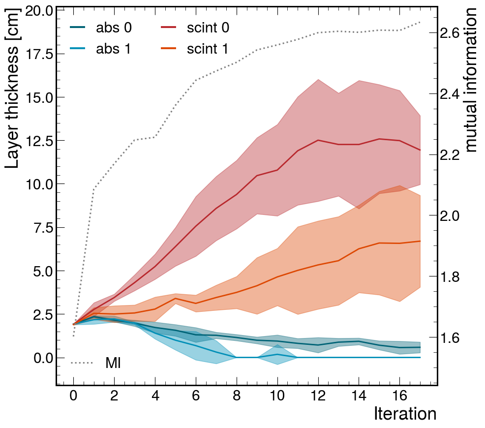
(c) MI-OPT, 2 layers

(d) RECO-OPT, 2 layers

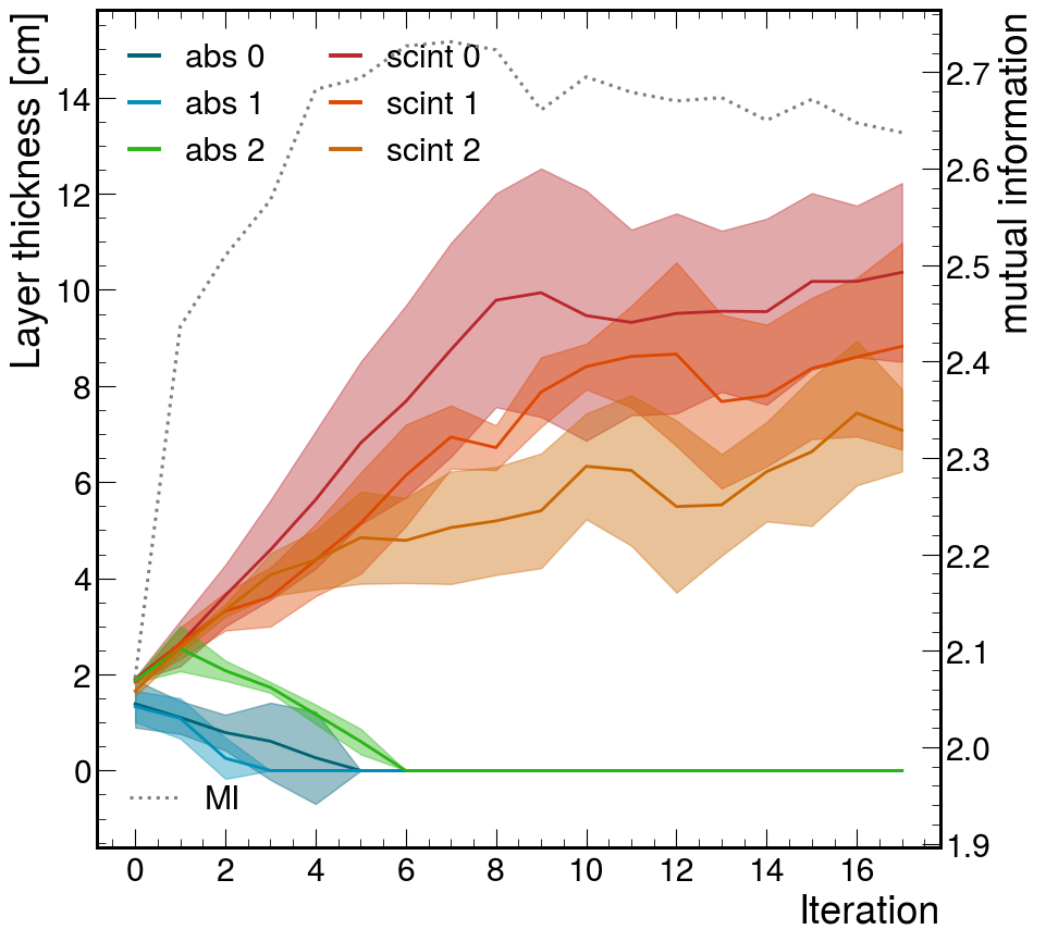
(e) MI-OPT, 3 layers

(f) RECO-OPT, 3 layers

Figure 3: BASE Study: Layer thickness evolution (solid lines) for MI-OPT (left, mutual information maximization in gray dashed) and RECO-OPT (right, reconstruction loss in gray solid, surrogate approximated loss in gray dashed), averaged over three runs for 1-layer (top), 2-layer (middle), and 3-layer (bottom) studies.

VI.1 Base Studies

The results of the base studies are shown in Figure 3. The left column displays data for the information theoretic approach MI-OPT while the right column displays data for the standard reconstruction based variant RECO-OPT.

In general, we observe that - as expected - both approaches maximize the scintillator segments while decreasing absorbers. In all tested settings, the absorbers are reduced either to zero or slightly above zero thicknesses, while the total gauge of scintillators increases beyond $20\text{\,}\mathrm{cm}$. Additionally, the scalar surrogate metric converges towards an optimum throughout the optimization iterations: mutual information increases in the MI-OPT studies (left column, dotted line), while the surrogate’s approximated reconstruction loss decreases in the RECO-OPT studies (right column, dotted line).

While MI-OPT increases the thickness of all available scintillators, RECO-OPT predominantly enhances only the first scintillator segment. This divergence can arise from the two approaches converging to distinct but functionally equivalent optima. As the optimization progresses and absorbers are effectively reduced to near-zero, the problem can be considered degenerate as segmentation of the scintillators becomes negligible if their total thicknesses sum to similar amounts (see Appendix B).
At the initial stages of optimization, both methods maintain at least one absorber with a nonzero thickness while the total scintillator thickness remains below a certain threshold. Absorbing material is discarded only once this limit is exceeded. This behavior reflects the necessity for sufficient energy containment within the calorimeter, ensuring maximal capture of the electromagnetic shower generated by the incident particle [44].
As the total gauge of the calorimeter is constrained (by adding a penalization term to the optimization of $\theta$ in the surrogate), we observe how both loss metrics plateau in RECO-OPT as the first scintillator thickness approaches $25\text{\,}\mathrm{c}\mathrm{m}$, while the mutual information metric plateaus in the three-layered study (Figure 3(e)) alongside scintillator thicknesses whose sum exceeds $25\text{\,}\mathrm{cm}$.

In conclusion, the results of the baseline experiment demonstrate that both optimization approaches successfully identify viable calorimeter designs that minmise or maximise their metric of choice across all case studies—ranging from single-layer to three-layer configurations—relying only on a scalar-valued objective function. The variations in the solutions are attributed to the existence of multiple optima in the objective function. This outcome highlights that an information-theoretic metric, despite offering a fundamentally different perspective on the problem, produces design choices closely aligned with those from traditional methods, confirming that state-of-the-art approaches are indeed operating near optimality.

The base studies were also performed for RECO-OPT using the diffusion based surrogate. A comparison of the single and three layer case to that of the 1D NF can be found in Appendix A.

VI.2 Transfer Learning

The impact of knowledge transfer with TL is illustrated in Figures 4 and 5, which present results for one- and three-layered calorimeters, respectively. Unlike the base studies discussed earlier, this experiment involves reinitializing the surrogate models (along with the reconstruction model in the case of RECO-OPT) at each iteration. Consequently, these models are exclusively trained on data in a local area of the parameter space, akin to the approach in [29].

A key observation is the increased fluctuation in the objective function (depicted by the grey dotted/solid lines). This behavior is expected, as the surrogates cannot accumulate knowledge to construct a smooth mapping of the $\theta-\delta$ landscape. In RECO-OPT, the losses stagnate or even increase, indicating a breakdown in the optimization process.

Without TL, RECO-OPT shows significantly increased variation in the evolution of one-layer studies and fails to converge to a solution for the three-layer problem (individual run plots are shown in the Appendix C). The deviation from results reported by [29] are attributed to the use of a fixed metric function which might contribute to stability in that study.
For MI-OPT, the effect of turning off TL leads to stagnation: the scintillator thickness plateaus at a lower value compared to the case where TL is enabled. For example, in the single-layer scenario (Figure 4(a)), the scintillator thickness remains below $10\text{\,}\mathrm{c}\mathrm{m}$ and absorber compression requires more iterations.
These findings highlight the effectiveness of TL in stabilizing the optimization process and guiding the search towards more optimal configurations, corroborating our hypothesis that a local surrogate can map out consecutive patches of the design parameter space in our framework setup.

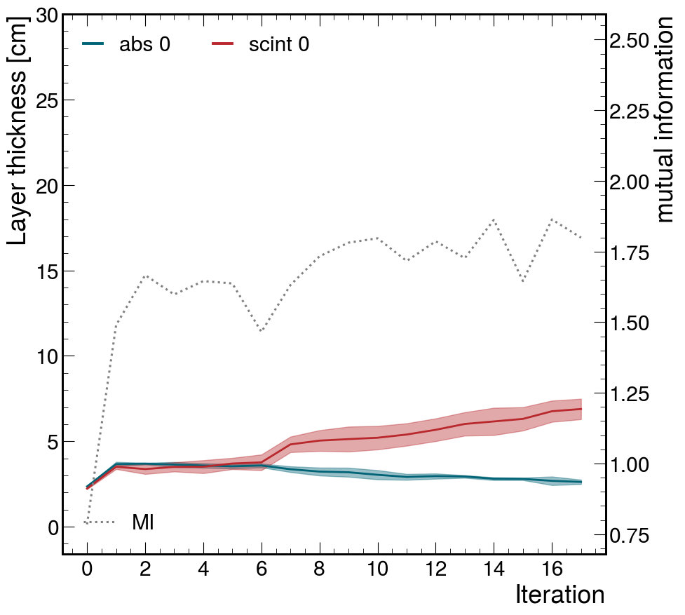
(a) MI-OPT, 1 layer, no TL, 700 events

(b) RECO-OPT, 1 layer, no TL, 700 events

Figure 4: TRANSFER study (700): Re-initialized learning (no transfer) with full sample size and a single layer calorimeter. Comparison of thickness evolutions for MI-OPT (left) and RECO-OPT (right) approaches.

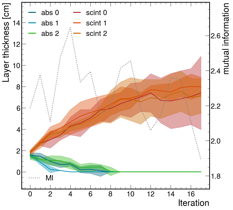
(a) MI-OPT, 3 layers, no TL, 700 events

(b) RECO-OPT, 3 layers, no TL, 700 events

Figure 5: TRANSFER study (700): Re-initialized learning (no transfer) with full sample size and three layers. Comparison of thickness evolutions for MI-OPT (left) and RECO-OPT (right) approaches.

To assess the relationship between TL and data sample size, we conducted experiments using just 50 simulated collision events per design parameter set. Note that the parameter neighborhood is sampled more densely in MI-OPT ($K=117$) than in RECO-OPT ($K=30$), such that the latter has access to a systematically smaller number of total samples. Preliminary studies were conducted showing that MI-OPT produces similar results with $K=50$, but in general, the information-theoretic metric relies more on adequate coverage of the true distributions of particle and sensor energies than the classic reconstruction approach.
We observe that, even with this limited data, both optimization approaches effectively increase scintillator thickness and reduce absorber thickness in a single-layer (Figure 6) and three-layer (Figure 7) calorimeter when TL is activated.

(a) MI-OPT, 1 layer, TL, 50 events

(b) RECO-OPT, 1 layer, TL, 50 events

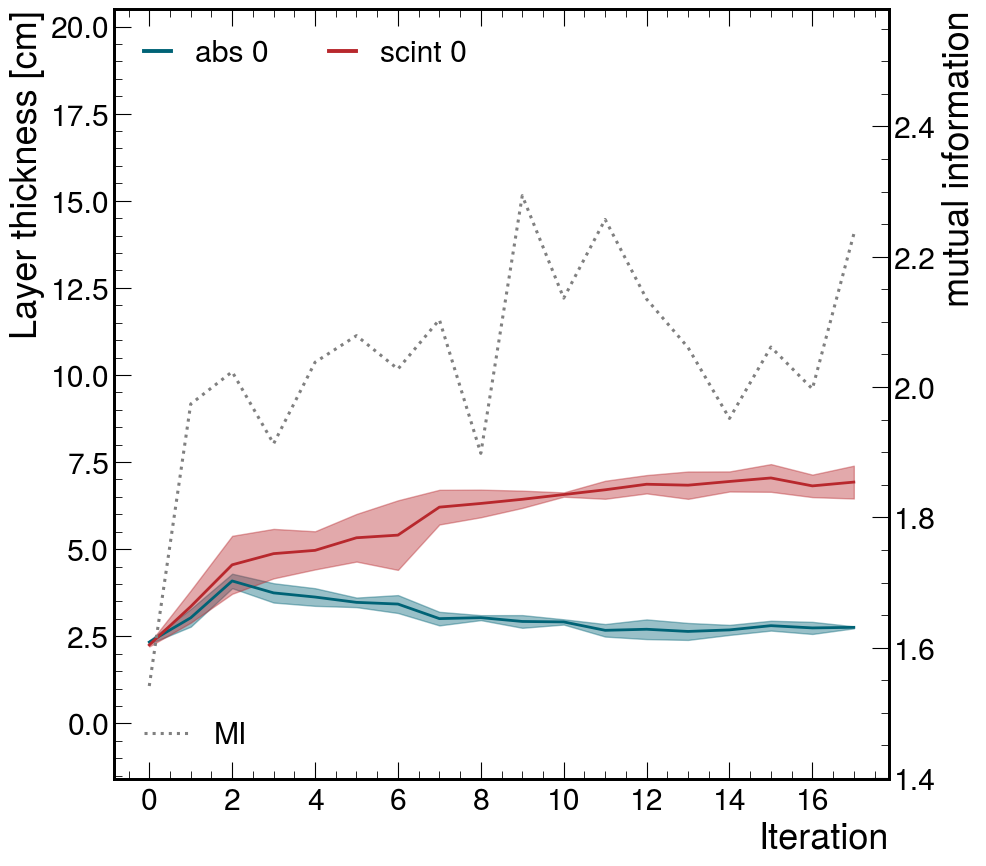
(c) MI-OPT, 1 layer, no TL, 50 events

(d) RECO-OPT, 1 layer, no TL, 50 events

Figure 6: TRANSFER study (50): Transfer learning studies with reduced sample size and one layer. Comparison of optimization evolutions with (top row) and without (bottom row) TL for mutual information (left column) and reconstruction (right column) approaches, with $50$ events per tested design parameter set.

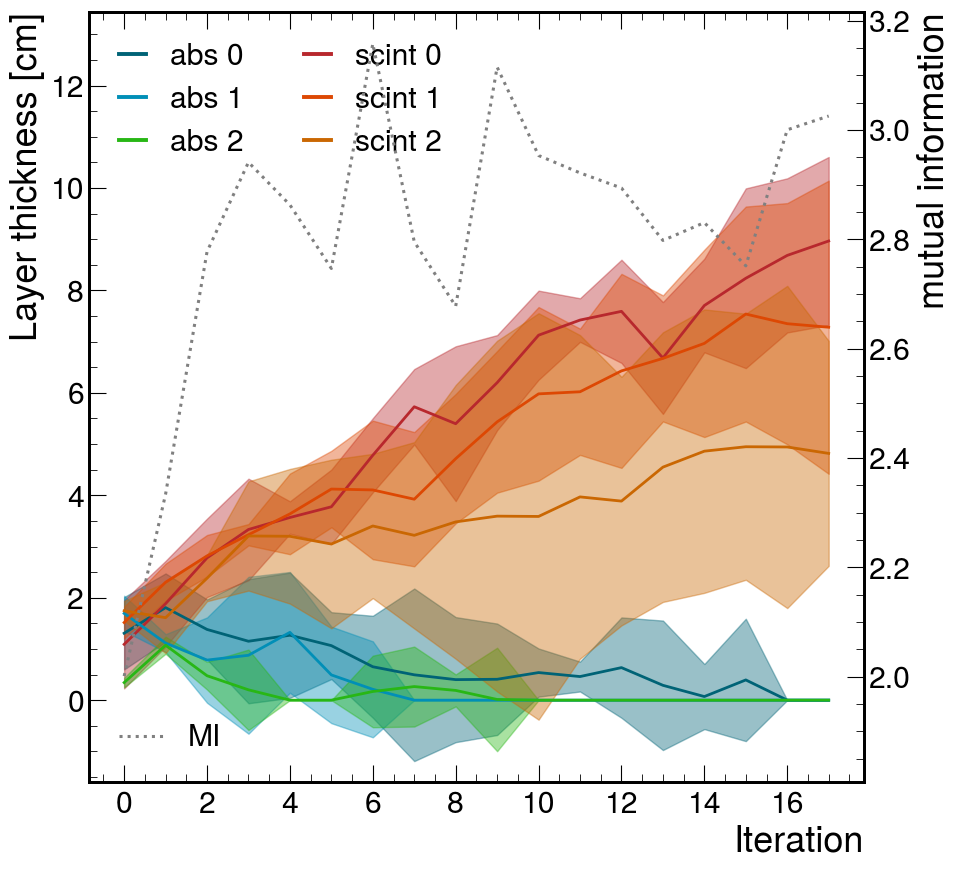
(a) MI-OPT, 3 layers, TL, 50 events

(b) RECO-OPT, 3 layers, TL, 50 events

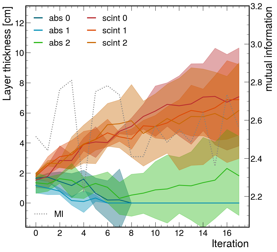
(c) MI-OPT, 3 layers, no TL, 50 events

(d) RECO-OPT, 3 layers, no TL, 50 events

Figure 7: TRANSFER study (50): Transfer learning studies with reduced sample size and three layers. Comparison of optimization evolutions with (top row) and without (bottom row) TL for mutual information (left column) and reconstruction (right column) approaches, with 50 events per parameter candidate.

The results are similar to the ones obtained with 700 events: For MI-OPT TL not only yields a much smoother mutual information metric but also leads to a different optimization trajectory. Both thickness values stagnate at a single-digit level when TL is not available. For RECO-OPT, we observe again a breakdown of optimization for the no-TL runs and a slower, but viable convergence when TL is present.

With RECO-OPT successfully converging with 50 events (Figure 6), we further reduce the event count to 5 (Figure 8), where optimization remains effective with TL but fails without it.

(a) RECO-OPT with TL, 5 events

(b) RECO-OPT without TL, 5 events

Figure 8: TRANSFER study (5): Transfer learning studies with reduced sample size and one layer. Comparison of optimization evolutions with (left) and without (right) TL for reconstruction metric, with $5$ events per tested design parameter set. Averaged over 10 runs.

It is notable how well the framework performs with TL at such low event numbers. Even when simulating $\mathcal{O}(10^{1})$ and $\mathcal{O}(10^{2})$ less events per variable the framework is still able to consistently converge to a similar final state as the base studies (Figure 3). Overall, these findings highlight the threshold at which sample size reduction begins to impede optimization performance and delineate the limits of TL. These observations have significant practical implications when extending the approaches to more complex, and slower simulation.

(a) MI-OPT, 1 layer, 700 events, [range-units=single,range-phrase=-]1100 GeV

(b) RECO-OPT, 1 layer, 700 events, [range-units=single,range-phrase=-]1100 GeV

(c) MI-OPT, 3 layers, 700 events, [range-units=single,range-phrase=-]1100 GeV

(d) RECO-OPT, 3 layers, 700 events, [range-units=single,range-phrase=-]1100 GeV

Figure 9: ENERGY study: Single and triple-paired calorimeter thickness evolution (solid lines) for MI-OPT (left, mutual information maximization shown by dotted line) and RECO-OPT (right, reconstruction loss minimization shown by dotted line), averaged over three runs for a photon with center of mass between [range-units=single,range-phrase=-]1100 GeV.

VI.3 Energy Studies

The results for the energy studies, where the energy range of the photon is increased to $100\text{\,}\mathrm{GeV}$, are shown in Figure 9.

We observe, that the absorber thickness, both in terms of its average value and variation bounds, remains consistently above that of the baseline scenario. For both algorithms and both layer settings, at least one absorber remains consistently above zero gauge. This outcome is expected, as a greater calorimeter thickness is necessary to effectively capture and measure the trajectories of higher-energy particles. Furthermore, the variability in scintillator thickness is consistently greater than in the baseline studies conducted with photon energies up to $20\text{\,}\mathrm{GeV}$. Also, notably, in the case of MI-OPT, the prioritization of layers is reversed, with the second scintillator exhibiting the most significant extension.

With increased energy, RECO-OPT continues to focus on increasing the width of the first scintillator primarily, though evolution proceeds at a lower rate. The scintillator thickness does not reach the $25\text{\,}\mathrm{c}\mathrm{m}$ constraint for neither the one nor three layer cases (Figures 9(b) and 9(d)), though it is trending towards that. With a significant number of higher energy events, a significantly lower fraction of the total energy of a given event is deposited in the calorimeter scintillators, making it difficult for the reconstruction network to learn and the surrogate as a whole to optimize the detector parameters.

VII Discussion

In this work, we presented a DL-based local surrogate framework for optimizing HEP detector designs using a scalar objective function. The optimization encompasses the forward as well as the inverse detector problem, yielding an end-to-end result.

Alongside a traditional reconstruction-based approach, we introduced a novel method leveraging the information-theoretic metric of mutual information as an optimization measure.

To evaluate the two frameworks, we conducted studies on a toy calorimeter model with one, two, and three layers, optimizing the thicknesses of absorber and scintillator components. Our results demonstrate that both approaches successfully optimize detector parameters, increasing scintillator thickness while reducing absorber thickness. This confirms that end-to-end, black-box DL-based optimization is feasible with only a single scalar objective function. In the case of our mutual information based optimization MI-OPT, this scalar objective function does not have to be specified explicitly, thus making it task-agnostic and user independent.

Our findings also support the effectiveness of progressive learning with TL in this context. The surrogate model accumulates knowledge about the design parameter space and the objective function landscape over the course of optimization. This is particularly evident in reduced data-sample settings, where strong optimization performance is achieved with as few as 50 events per parameter candidate for both frameworks, and 5 events per parameter candidate for the standard optimization RECO-OPT. In contrast, without TL, optimization results remain suboptimal or the optimization process completely fails, highlighting the benefits of leveraging prior knowledge in iterative design processes. The ability to achieve comparable optimization performance for orders of magnitude fewer simulation calls is desirable as the simulation step is often a bottleneck for optimization tasks.

For future work, incorporating both energy resolution and particle classification accuracy as an additional objective, the framework could optimize detector designs for multi-objective tasks, reflecting the real-world challenges of HEP detector development.

Our findings show that mutual information produces design choices closely aligned with state-of-the-art physics-informed methods, suggesting these approaches operate near optimality. Beyond validating existing methods, mutual information enables broader exploration and generalization of the optimization process, as it is inherently problem-agnostic, though at the cost of increased computational demands. By shifting the focus from domain-specific heuristics to an information-theoretic formulation, this approach opens new avenues for exploring design spaces beyond conventional methodologies.

Appendix A One-Dimensional flow vs Diffusion

While the diffusion models generally in this case have lower run-to-run variation, the 1D NF provides gains in terms of runtime due to significantly simpler architecture and training procedure. For a comparison of the evolution of a single layer optimization see Figure 10(a).

(a) One-dimensional flow model evolution, 1 layer

(b) Diffusion model evolution, 1 layer

(c) One-dimensional flow model evolution, 3 layers

(d) Diffusion model evolution, 3 layers

Figure 10: Comparison of one-dimensional flow and diffusion model for one and three layers with 700 events and photons between $1\text{\,}\mathrm{a}$nd $20\text{\,}\mathrm{G}\mathrm{e}\mathrm{V}$.

Appendix B Summation of Layer Thickness

When summing total scintillator and absorber thickness we see that generally the total scintillator thickness approaches the constraint of $25\text{\,}\mathrm{c}\mathrm{m}$ while the total absorber thickness approaches $0\text{\,}\mathrm{c}\mathrm{m}$, shown in Figure 11.

(a) Sum 2 layers, MI-OPT

(b) Sum 2 layers, RECO-OPT

(c) Sum 3 layers, MI-OPT

(d) Sum 3 layers, RECO-OPT

Figure 11: Summation of layer thickness evolution for MI-OPT (left) and RECO-OPT (right), averaged over three runs for the 2 layer (top row), and 3 layer (bottom row) calorimeters. All runs use 700 events with incident energy ranging between [range-units=single,range-phrase=-]120 GeV.

Appendix C Failure Cases without Transfer Learning

For RECO-OPT, the use of TL seems to be essential for reasonable and consistent performance. Without TL, even for relatively large event numbers, a breakdown in the optimization process is observed. Individual runs fail in distinct ways, which can make the run-averaged plots for these cases difficult to interpret. Here the evolutions of the individual runs are presented for reference. Individual runs of cases using TL are displayed in Figure 12 and without TL in Figure 13.

Using TL, the evolutions regardless of the number of simulated events are very similar, all beginning with some small increase in absorber thickness before beginning to increase scintillator thickness.

Without TL, the behaviour is quite different. For 700 events, we see very inconsistent behaviour, often achieving large and nonphysical values. When reducing to 50 and 5 events, we see a repeated pattern of failure where both segments are increased uniformly until $\sim$ $13\text{\,}\mathrm{c}\mathrm{m}$, when either the scintillator or absorber will continue to increase or begin to decrease. These failure cases are not well understood but are clearly linked to the lack of TL.

(a) 700 events, run 0

(b) 700 events, run 1

(c) 700 events, run 2

(d) 50 events, run 0

(e) 50 events, run 1

(f) 50 events, run 2

(g) 5 events, run 0

(h) 5 events, run 1

(i) 5 events, run 2

Figure 12: RECO-OPT: Individual runs with TL. Top row shows 700 events, middle shows 50 events, bottom shows 5 events.

(a) 700 events, run 0

(b) 700 events, run 1

(c) 700 events, run 2

(d) 50 events, run 0

(e) 50 events, run 1

(f) 50 events, run 2

(g) 5 events, run 0

(h) 5 events, run 1

(i) 5 events, run 2

Figure 13: RECO-OPT: Individual runs without TL. Top row shows 700 events, middle shows 50 events, bottom shows 5 events.

Appendix D Experiment and Network Hyperparameters

The hyperparameters used by the reconstruction and surrogate models of each framework are presented in Table 3. The networks in RECO-OPT go through different training stages with reduced learning rates (LR). The reconstruction network is trained for 200 epochs with LR $4\times 10^{-4}$ and then 200 epochs at $1\times 10^{-5}$, while the surrogate network starts with $3\times 10^{-4}$, then $1\times 10^{-4}$, and finally $1\times 10^{-5}$, each for 200 epochs. The 1D NF uses an MLP to predict the piecewise linear parameters based on the conditional parameters. The number of MLP layers and activation function listed in the table for RECO-OPT Surr are the hyperparameters of this MLP.

Hyperparameters
Networks	N MLP Layers	Activation	LR	Epochs	Optimizer
RECO-OPT Reco	3	ELU [57]	$4\times 10^{-4}$ / $1\times 10^{-5}$	400	ADAM [58]
RECO-OPT Surr			$3\cdot 10^{-4}$ / $1\times 10^{-4}$ / $1\times 10^{-5}$	600
MI-OPT Reco	encoder + decoder: 3 + MLP: 2		scheduler (init $1\cdot 10^{-2}$)	2000
MI-OPT Surr	4		scheduler (init $5\cdot 10^{-2}$)	150

Table 3: Network hyperparameters

References

- Apollinari et al. [2017] G. Apollinari et al., High-Luminosity Large Hadron Collider (HL-LHC). Technical Design Report V. 0.1, Tech. Rep. (Fermi National Accelerator Lab. (FNAL), Batavia, IL (United States), 2017).
- The FCC Collaboration [2019] The FCC Collaboration, Fcc-hh: The hadron collider: Future circular collider conceptual design report volume 3, European Physical Journal Special Topics 228, 755 (2019).
- Jones et al. [1998] D. R. Jones, M. Schonlau, and W. J. Welch, Efficient global optimization of expensive black-box functions, Journal of Global Optimization 13, 455 (1998).
- Dorigo et al. [2025] T. Dorigo, M. Doro, M. Aehle, N. R. Gauger, M. Awais, R. Izbicki, J. Kieseler, L. Masserano, F. Nardi, and L. R. Vergara, On the utility function of experiments in fundamental science (2025), arXiv:2501.13544 [hep-ex] .
- Aehle et al. [2024a] M. Aehle, X. T. Nguyen, M. Novák, T. Dorigo, N. R. Gauger, J. Kieseler, M. Klute, and V. Vassilev, Efficient forward-mode algorithmic derivatives of geant4 (2024a), arXiv:2407.02966 [physics.comp-ph] .
- Aehle et al. [2024b] M. Aehle, M. Novák, V. Vassilev, N. R. Gauger, L. Heinrich, M. Kagan, and D. Lange, Optimization using pathwise algorithmic derivatives of electromagnetic shower simulations (2024b), arXiv:2405.07944 [physics.comp-ph] .
- Kagan and Heinrich [2023] M. Kagan and L. Heinrich, Branches of a tree: Taking derivatives of programs with discrete and branching randomness in high energy physics (2023), arXiv:2308.16680 [stat.ML] .
- Dorigo et al. [2024] T. Dorigo, M. Aehle, C. Arcaro, M. Awais, F. Bergamaschi, J. Donini, M. Doro, N. R. Gauger, R. Izbicki, J. Kieseler, A. Lee, L. Masserano, F. Nardi, R. Rajesh, L. R. Vergara, and A. Shen, Toward the end-to-end optimization of the swgo array layout (2024), arXiv:2310.01857 [astro-ph.IM] .
- Baydin et al. [2021] A. G. Baydin et al., Toward machine learning optimization of experimental design, Nuclear Physics News 31, 25 (2021), https://doi.org/10.1080/10619127.2021.1881364 .
- Dorigo et al. [2023] T. Dorigo et al., Toward the end-to-end optimization of particle physics instruments with differentiable programming, Reviews in Physics 10, 100085 (2023).
- Strong et al. [2024] G. Strong et al., Tomopt: differential optimisation for task- and constraint-aware design of particle detectors in the context of muon tomography, Machine Learning: Science and Technology 5, 035002 (2024).
- Qasim et al. [2024] S. R. Qasim, P. Owen, and N. Serra, Physics instrument design with reinforcement learning (2024), arXiv:2412.10237 [physics.ins-det] .
- Kortus et al. [2025] T. Kortus, R. Keidel, N. R. Gauger, and J. Kieseler, Constrained optimization of charged particle tracking with multi-agent reinforcement learning (2025), arXiv:2501.05113 [physics.comp-ph] .
- Golovin et al. [2017] D. Golovin, G. Kochanski, and J. E. Karro, Black box optimization via a bayesian-optimized genetic algorithm, in Advances in Neural Information Processing Systems 30 (NIPS 2017) (2017) to be submitted to Opt2017 Optimization for Machine Learning, at NIPS 2017.
- Hofler et al. [2013] A. Hofler, B. c. v. Terzić, M. Kramer, A. Zvezdin, V. Morozov, Y. Roblin, F. Lin, and C. Jarvis, Innovative applications of genetic algorithms to problems in accelerator physics, Phys. Rev. ST Accel. Beams 16, 010101 (2013).
- Geisel et al. [2013] I. Geisel et al., Evolutionary optimization of an experimental apparatus, Applied Physics Letters 102, 214105 (2013), https://pubs.aip.org/aip/apl/article-pdf/doi/10.1063/1.4808213/14276514/214105_1_online.pdf .
- Rolla et al. [2023] J. Rolla, A. Machtay, A. Patton, W. Banzhaf, A. Connolly, R. Debolt, L. Deer, E. Fahimi, E. Ferstle, P. Kuzma, C. Pfendner, B. Sipe, K. Staats, and S. A. Wissel (GENETIS Collaboration), Using evolutionary algorithms to design antennas with greater sensitivity to ultrahigh energy neutrinos, Phys. Rev. D 108, 102002 (2023).
- Shahriari [2016] B. e. a. Shahriari, Taking the human out of the loop: A review of bayesian optimization, Proceedings of the IEEE 104, 148 (2016).
- Eriksson et al. [2019] D. Eriksson, M. Pearce, J. Gardner, R. D. Turner, and M. Poloczek, Scalable global optimization via local bayesian optimization, in Advances in Neural Information Processing Systems, Vol. 32, edited by H. Wallach, H. Larochelle, A. Beygelzimer, F. d'Alché-Buc, E. Fox, and R. Garnett (Curran Associates, Inc., 2019).
- Wu et al. [2023] K. Wu, K. Kim, R. Garnett, and J. R. Gardner, The behavior and convergence of local bayesian optimization, in Proceedings of the 37th International Conference on Neural Information Processing Systems, NIPS ’23 (Curran Associates Inc., Red Hook, NY, USA, 2023).
- Nguyen et al. [2022] Q. Nguyen, K. Wu, J. R. Gardner, and R. Garnett, Local bayesian optimization via maximizing probability of descent, Advances in neural information processing systems abs/2210.11662 (2022).
- Zhang et al. [2020] Y. Zhang, D. Apley, and W. Chen, Bayesian optimization for materials design with mixed quantitative and qualitative variables, Scientific Reports 10 (2020).
- Khatamsaz et al. [2023] D. Khatamsaz et al., A physics informed bayesian optimization approach for material design: application to niti shape memory alloys, npj Computational Materials 9 (2023).
- Nicoli et al. [2023] K. A. Nicoli et al., Physics-informed bayesian optimization of variational quantum circuits, in Proceedings of the 37th International Conference on Neural Information Processing Systems, NIPS ’23 (Curran Associates Inc., Red Hook, NY, USA, 2023).
- Grbcic et al. [2025] L. Grbcic et al., Artificial intelligence driven laser parameter search: Inverse design of photonic surfaces using greedy surrogate-based optimization, Engineering Applications of Artificial Intelligence 143, 109971 (2025).
- Elzouka et al. [2020] M. Elzouka et al., Interpretable forward and inverse design of particle spectral emissivity using common machine-learning models, Cell Reports Physical Science 1 (2020).
- Fanelli [2022] C. Fanelli, Design of detectors at the electron ion collider with artificial intelligence, Journal of Instrumentation 17 (04), C04038.
- Hashemi and Krause [2024] B. Hashemi and C. Krause, Deep generative models for detector signature simulation: A taxonomic review, Reviews in Physics 12, 100092 (2024).
- Shirobokov et al. [2020] S. Shirobokov, V. Belavin, M. Kagan, A. Ustyuzhanin, and A. G. Baydin, Black-box optimization with local generative surrogates, in Advances in Neural Information Processing Systems, Vol. 33, edited by H. Larochelle, M. Ranzato, R. Hadsell, M. Balcan, and H. Lin (Curran Associates, Inc., 2020) pp. 14650–14662.
- Schmidt et al. [2025] K. Schmidt, N. Kota, J. Kieseler, A. D. Vita, M. Klute, Abhishek, M. Aehle, M. Awais, A. Breccia, R. Carroccio, L. Chen, T. Dorigo, N. R. Gauger, E. Lupi, F. Nardi, X. T. Nguyen, F. Sandin, J. Willmore, and P. Vischia, End-to-end detector optimization with diffusion models: A case study in sampling calorimeters (2025), arXiv:2502.02152 [physics.ins-det] .
- Neiswanger et al. [2021] W. Neiswanger, K. A. Wang, and S. Ermon, Bayesian algorithm execution: Estimating computable properties of black-box functions using mutual information, in International Conference on Machine Learning (ICML) (2021).
- Chitturi et al. [2024] S. R. Chitturi, A. Ramdas, Y. Wu, B. Rohr, S. Ermon, J. Dionne, F. H. d. Jornada, M. Dunne, C. Tassone, W. Neiswanger, and D. Ratner, Targeted materials discovery using bayesian algorithm execution, npj Computational Materials 10, 10.1038/s41524-024-01326-2 (2024).
- MacKay [2002] D. J. C. MacKay, Information Theory, Inference & Learning Algorithms (Cambridge University Press, USA, 2002).
- Cover [1999] T. M. Cover, Elements of information theory (John Wiley & Sons, 1999).
- Bitbol [2018] A.-F. Bitbol, Inferring interaction partners from protein sequences using mutual information, PLoS Computational Biology 14 (2018).
- Paninski [2003] L. Paninski, Estimation of entropy and mutual information, Neural Computation 15, 1191 (2003), https://direct.mit.edu/neco/article-pdf/15/6/1191/815550/089976603321780272.pdf .
- Bahl et al. [1986] L. Bahl, P. Brown, P. Souza, and R. Mercer, Maximum mutual information estimation of hidden markov parameters for speech recognition, in ICASSP, IEEE International Conference on Acoustics, Speech and Signal Processing - Proceedings, Vol. 11 (1986) pp. 49 – 52.
- Church and Hanks [1990] K. W. Church and P. Hanks, Word association norms, mutual information, and lexicography, Computational Linguistics 16, 22 (1990).
- Agostinelli et al. [2003] S. Agostinelli et al., Geant4—a simulation toolkit, Nuclear Instruments and Methods in Physics Research Section A: Accelerators, Spectrometers, Detectors and Associated Equipment 506, 250 (2003).
- Allison et al. [2006] J. Allison et al., Geant4 developments and applications, IEEE Transactions on Nuclear Science 53, 270 (2006).
- Allison et al. [2016] J. Allison et al., Recent developments in geant4, Nuclear Instruments and Methods in Physics Research Section A: Accelerators, Spectrometers, Detectors and Associated Equipment 835, 186 (2016).
- Aleksandrov et al. [2005] D. Aleksandrov et al., A high resolution electromagnetic calorimeter based on lead-tungstate crystals, Nuclear Instruments and Methods in Physics Research Section A: Accelerators, Spectrometers, Detectors and Associated Equipment 550, 169 (2005).
- Lecoq et al. [1995] P. Lecoq et al., Lead tungstate (pbwo4) scintillators for lhc em calorimetry, Nuclear Instruments and Methods in Physics Research Section A: Accelerators, Spectrometers, Detectors and Associated Equipment 365, 291 (1995).
- Bandiera et al. [2023] L. Bandiera et al., A highly-compact and ultra-fast homogeneous electromagnetic calorimeter based on oriented lead tungstate crystals, Frontiers in Physics 11, 10.3389/fphy.2023.1254020 (2023).
- Sorensen [1982] D. C. Sorensen, Newton’s method with a model trust region modification, SIAM Journal on Numerical Analysis 19, 409 (1982), https://doi.org/10.1137/0719026 .
- Kraskov et al. [2004] A. Kraskov, H. Stögbauer, and P. Grassberger, Estimating mutual information, Phys. Rev. E 69, 066138 (2004).
- Rezende and Mohamed [2016] D. J. Rezende and S. Mohamed, Variational inference with normalizing flows (2016), arXiv:1505.05770 [stat.ML] .
- Kobyzev et al. [2021] I. Kobyzev, S. J. Prince, and M. A. Brubaker, Normalizing flows: An introduction and review of current methods, IEEE Transactions on Pattern Analysis and Machine Intelligence 43, 3964–3979 (2021).
- Papamakarios et al. [2021] G. Papamakarios, E. Nalisnick, D. J. Rezende, S. Mohamed, and B. Lakshminarayanan, Normalizing flows for probabilistic modeling and inference, Journal of Machine Learning Research 22, 1 (2021).
- Winkler et al. [2023] C. Winkler, D. Worrall, E. Hoogeboom, and M. Welling, Learning likelihoods with conditional normalizing flows (2023), arXiv:1912.00042 [cs.LG] .
- Müller et al. [2019] T. Müller, B. McWilliams, F. Rousselle, M. Gross, and J. Novák, Neural importance sampling (2019), arXiv:1808.03856 [cs.LG] .
- Belghazi et al. [2018] M. I. Belghazi et al., Mutual information neural estimation, in Proceedings of the 35th International Conference on Machine Learning, Proceedings of Machine Learning Research, Vol. 80, edited by J. Dy and A. Krause (PMLR, 2018) pp. 531–540.
- Hjelm et al. [2019] R. D. Hjelm, A. Fedorov, S. Lavoie-Marchildon, K. Grewal, P. Bachman, A. Trischler, and Y. Bengio, Learning deep representations by mutual information estimation and maximization, in International Conference on Learning Representations (2019).
- Zhuang et al. [2019] F. Zhuang et al., A comprehensive survey on transfer learning, CoRR abs/1911.02685 (2019), 1911.02685 .
- Mokhtar et al. [2025] F. Mokhtar, J. Pata, M. Kagan, D. Garcia, E. Wulff, M. Zhang, and J. Duarte, Fine-tuning machine-learned particle-flow reconstruction for new detector geometries in future colliders (2025), arXiv:2503.00131 [hep-ex] .
- de Fatis and behalf of the CMS Collaboration) [2012] T. T. de Fatis and O. behalf of the CMS Collaboration), Role of the cms electromagnetic calorimeter in the hunt for the higgs boson in the two-gamma channel, Journal of Physics: Conference Series 404, 012002 (2012).
- Clevert et al. [2016] D.-A. Clevert, T. Unterthiner, and S. Hochreiter, Fast and accurate deep network learning by exponential linear units (elus) (2016), arXiv:1511.07289 [cs.LG] .
- Kingma and Ba [2017] D. P. Kingma and J. Ba, Adam: A method for stochastic optimization (2017), arXiv:1412.6980 [cs.LG] .