Higher-Order Graphon Neural Networks:
Approximation and Cut Distance

Abstract

Graph limit models, like graphons for limits of dense graphs, have recently been used to study size transferability of graph neural networks (GNNs). While most literature focuses on message passing GNNs (MPNNs), in this work we attend to the more powerful higher-order GNNs. First, we extend the $k$-WL test for graphons (Böker, 2023) to the graphon-signal space and introduce signal-weighted homomorphism densities as a key tool. As an exemplary focus, we generalize Invariant Graph Networks (IGNs) to graphons, proposing Invariant Graphon Networks (IWNs) defined via a subset of the IGN basis corresponding to bounded linear operators. Even with this restricted basis, we show that IWNs of order $k$ are at least as powerful as the $k$-WL test, and we establish universal approximation results for graphon-signals in $L^{p}$ distances. This significantly extends the prior work of Cai & Wang (2022), showing that IWNs—a subset of their IGN-small—retain effectively the same expressivity as the full IGN basis in the limit. In contrast to their approach, our blueprint of IWNs also aligns better with the geometry of graphon space, for example facilitating comparability to MPNNs. We highlight that, while typical higher-order GNNs are discontinuous w.r.t. cut distance—which causes their lack of convergence and is inherently tied to the definition of $k$-WL—their transferability remains comparable to MPNNs.

1 Introduction

Graph Neural Networks (GNNs) have emerged as a powerful tool for machine learning on complex graph-structured data, driving advances in fields like social network analysis (Fan et al., 2019), weather prediction (Lam et al., 2023) or materials discovery (Merchant et al., 2023). Message Passing GNNs (MPNNs) (Gilmer et al., 2017; Kipf & Welling, 2017; Veličković et al., 2018; Xu et al., 2019), which update node features by neighborhood aggregations, are a popular paradigm.

The question of size transferability—whether an MPNN generalizes to larger graphs than those in the training set—has recently gained attention. Unlike extrapolation (Xu et al., 2021; Yehudai et al., 2021; Jegelka, 2022), where generalization to arbitrary graph topologies is considered, size transferability typically assumes structural similarities between the training and evaluation graphs, such as them being sampled from the same random graph model (Keriven et al., 2021), topological space (Levie et al., 2021), or graph limit model (Ruiz et al., 2020; 2023; 2021b; Maskey et al., 2024; Le & Jegelka, 2024). For limits of dense graphs, graphons (Lovász & Szegedy, 2006; Lovász, 2012), which extend graphs to node sets on the unit interval and have been used to study extremal graph theory with analytic techniques, have also become a popular choice for studying transferability. In contrast to sparse graph limits (Lovász, 2012; Backhausz & Szegedy, 2022), they offer an established framework with powerful tools, such as embedding the set of all graphs into a compact space and having favorable spectral properties (Ruiz et al., 2021a). In such transferability analyses, a GNN is extended to a function of graphons, and regularity properties of the GNN are then used to bound the difference between outputs of the GNN applied to samples of different sizes from a graphon.

Existing works on transferability have been almost exclusively limited to MPNNs. However, their expressive power is constrained by the 1-dimensional Weisfeiler-Leman graph isomorphism test (1-WL), also known as the color refinement algorithm (Xu et al., 2019; Morris et al., 2019). Hence, standard MPNNs even fail at straightforward tasks such as counting simple patterns like cycles. This motivates extending generalization analyses to more powerful architectures. Most prominent among these are higher-order extensions of MPNNs that are as powerful as the $k$-WL test, $k>1$, which iteratively colors $k$-tuples of nodes (Morris et al., 2019). Invariant and Equivariant Graph Networks (IGNs/EGNs) (Maron et al., 2018), which serve as an exemplary focus in this work, are a popular architectural choice, in which adjacency matrices and node signals are processed through higher-order tensor operations that maintain permutation equivariance. IGNs/EGNs universally approximate any permutation in-/equivariant graph function, and are as powerful as $k$-WL with orders $\leq k$ (Maron et al., 2019b; Keriven & Peyré, 2019; Maehara & NT, 2019; Azizian & Lelarge, 2021).

The expressive power of a GNN can also be judged via its homomorphism expressivity, i.e., its ability to count the number of homomorphisms from fixed graphs into the input graph. E.g., 1-WL corresponds to counting homomorphisms w.r.t. trees, and its higher-order extensions are related to counting homomorphisms w.r.t. graphs of bounded treewidth (Dvořák, 2010; Dell et al., 2018). In the graphon case, similar results exist for homomorphism densities (Böker et al., 2023; Böker, 2023).

In this work, we study expressivity, continuity, and transferability properties of higher-order GNN extensions to graphons. Maehara & NT (2019) note that their IGN/EGN universality proof—using a parametrization relying on explicit simple homomorphism densities—extends to graphons. They regard the use of graphons for such analyses as promising. The closest related work by Cai & Wang (2022) investigates the convergence of IGNs to a limit graphon via a partition norm—a vector of norms over all diagonals of a graphon. They observe that IGNs on graphon-sampled graphs do not always converge. They propose a reduced model class IGN-small, which enables convergence after estimating edge probabilities under certain regularity conditions. They also demonstrate that IGN-small retains sufficient expressiveness to approximate spectral GNNs. However, we argue that considering diagonals of graphons (i.e., null sets in Lebesgue measure) is somewhat misaligned with the larger body of work in graphon theory, significantly limiting its applicability to their version of IGN limits. Furthermore, their expressivity analysis of IGN-small is rather limited, given that IGNs are typically universal GNN architectures.

Contributions. A first focus of this work is to extend the $k$-WL test (Böker, 2023) and homomorphism densities from graphons to graphon-signals (Levie, 2023), i.e., node-attributed graphons. For the extension of homomorphism densities, we introduce signal weighting and show that signal-weighted homomorphism densities inherit most topological properties from their graphon equivalent.

We generalize IGNs to graphon-signals, introducing Invariant Graphon Networks (IWNs). In contrast to Cai & Wang (2022), we restrict linear equivariant layers to bounded operators, and, thus, our IWNs can be analyzed using $L^{p}$ and cut distances, enhancing comparability to the existing graphon literature. Using only this reduced basis, we show that IWNs of order up to $k$ are as powerful as the $k$-WL test for graphon-signals and we establish universal approximation results in $L^{p}$ distances. As IWNs are a subset of IGN-small, this significantly extends the work of Cai & Wang (2022), resolving the open questions posed in their conclusion: We show that the restriction to IGN-small comes at no cost in terms of expressivity. We carry out expressivity analyses using our notion of homomorphism expressivity via signal-weighted homomorphism densities. IWNs are discontinuous w.r.t. the cut distance and only continuous in the finer topologies induced by $L^{p}$ distances, which do not represent our intuitive notion of graph similarity (Levie, 2023). This discontinuity is not unique to IWNs, but inherently tied to the way in which $k$-WL processes edge weights, and results in a large class of higher-order GNNs defined via color refinement exhibiting an absence of convergence under sampling simple graphs. Yet, despite this discontinuity, it is still possible to obtain transferability results for higher-order GNNs which are similar to MPNNs.

To the best of our knowledge, this work is the first to extend higher-order GNNs to graphons in a way that facilitates a systematic study of continuity, expressivity, and transferability in comparison to MPNNs, addressing the aforementioned challenges of Cai & Wang (2022) while building on the foundational work of Böker (2023). In summary, we make the following contributions:

• We define signal-weighted homomorphism densities, link them to a natural extension of the $k$-WL test to graphon-signals, and show how they capture graphon-signal topology.

• We introduce Invariant Graphon Networks (IWNs), restricting linear equivariant layers to bounded operators. We show that IWNs of order $k$ are at least as powerful as $k$-WL for graphon-signals, and establish universal approximation, extending Cai & Wang (2022).

• We point out the cut distance discontinuity of typical higher-order GNNs and demonstrate that such models are still transferable despite not converging to their graphon limit.

2 Background

In this section, we provide background on graphon theory, homomorphism expressivity, and the $k$-WL test for graphons, as well as on how to extend graphons to incorporate node signals. Contents of subsection 2.1 and subsection 2.2 are mostly drawn from Lovász (2012); Janson (2013); Zhao (2023), while in subsection 2.2 we also refer to Böker (2023). In subsection 2.3 we summarize key results of Levie (2023).

For $n\in\mathbb{N}$, write $[n]:=\{1,\dots,n\}$. Unless stated otherwise, a graph always refers to a simple graph, meaning an undirected graph $G=(V,E)$ with a finite node set $V(G)=V$ and edge set $E(G)=E\subseteq\binom{V}{2}$. Define also $v(G):=\left|{V(G)}\right|$, $e(G):=\left|{E(G)}\right|$. We will also consider multigraphs, for which the edges are a multiset. Write $\lambda^{k}$ for the $k$-dimensional Lebesgue measure; $\lambda:=\lambda^{1}$. See Appendix A for a table of notation and subsection B.1 for background on topology and measure theory.

2.1 General Background on Graphon Theory

Graphons.

Informally, a graphon can be seen as a graph with a continuous node set $[0,1]$, and the adjacency matrix being represented by a function on the unit square. Intuitively, graphons can be obtained by taking the limit of adjacency matrices of dense graph sequences as the number of nodes grows. Formally, we first define a kernel as a bounded symmetric measurable function $W:[0,1]^{2}\to\mathbb{R}$. Write $\mathcal{W}$ for the space of all kernels. A graphon is a kernel mapping to $[0,1]$. We define the cut norm of a kernel as

$$\|{W}\|_{\square}:=\sup_{S,T\subseteq[0,1]}\left|{\int_{S\times T}W\mathrm{d}\lambda^{2}}\right|,$$ (1)

where $S,T$ are tacitly assumed measurable. Let $S_{[0,1]}$ be the set of measure-preserving maps $\varphi:[0,1]\to[0,1]$ that are bijective almost everywhere; that is, for every measurable $A\subseteq[0,1]$, we have $\lambda(\varphi^{-1}(A))=\lambda(A)$. Write $\overline{S}_{[0,1]}$ for the set of all measure preserving functions and define $W^{\varphi}(x,y)\,:=\,W(\varphi(x),\varphi(y))$ for $\varphi\in\overline{S}_{[0,1]}$. Since the specific ordering of the graphon values does not matter, we work with the cut distance (Lovász, 2012, § 8.2) between two graphons, defined as

$$\delta_{\square}(W,V)\,:=\,\inf_{\varphi\in S_{[0,1]}}\|{W-V^{\varphi}}\|_{\square}\,=\,\min_{\varphi,\psi\in\overline{S}_{[0,1]}}\|{W^{\varphi}-V^{\psi}}\|_{\square},$$ (2)

where the infimum is only guaranteed to be attained in the latter expression. Analogously, we can define distances $\delta_{p}$ on graphons based on $L^{p}$ norms, $p\in[1,\infty]$. Note that $\delta_{\square}\leq\delta_{1}$ (which follows from moving $\left|{\cdot}\right|$ into the integral in (1)) and $\delta_{p}\leq\delta_{q}$ for $p\leq q$. $\delta_{\square}$ and $\{\delta_{p}\}_{p}$, $p<\infty$, vanish simultaneously. However, the topology induced by $\delta_{\square}$ is strictly coarser than that induced by $\{\delta_{p}\}_{p\in[1,\infty)}$ (all of which coincide), which is in turn coarser than the topology induced by $\delta_{\infty}$. The most commonly used among $\{\delta_{p}\}_{p}$ is $\delta_{1}$, which corresponds (up to a constant; see Lovász (2012, § 9)) to the edit distance on graphs. We identify weakly isomorphic graphons of distance 0 to form the space $\widetilde{\mathcal{W}}_{0}$ of unlabeled graphons. The stricter concept of (strong) isomorphism, namely that the minimum over $S_{[0,1]}$ in (2) is attained and zero, is less practical. The usefulness of $\delta_{\square}$ over any $\delta_{p}$ lies in the fact that $(\widetilde{\mathcal{W}}_{0},\delta_{\square})$ forms a compact space (Lovász, 2012, Theorem 9.23).

Discretization and sampling.

Any labeled graph $G$ can be identified with its induced step graphon $W_{G}:=\sum_{j=1}^{n}\sum_{k=1}^{n}{A}_{jk}\mathds{1}_{I_{j}\times I_{k}}$ for a regular partition $\{I_{j}\}_{j=1}^{n}$ of the unit interval, and finite graphs are dense in the graphon space (Zhao, 2023, Theorem 4.2.8). Graphons can also be seen as random graph models: Draw $\mathbf{X}\sim U(0,1)^{n}$, and let $W({\bm{X}})$ be a graph with edge weights ${W}_{ij}=W(X_{i},X_{j})$. If $e_{ij}\sim\mathrm{Bernoulli}(W_{ij})$ is further sampled, we obtain an unweighted graph $\mathbb{G}(W,{\bm{X}})$. Write $\mathbb{H}_{n}(W)$ and $\mathbb{G}_{n}(W)$ for the respective distributions. We have $\delta_{\square}(\mathbb{H}_{n}(W),W)\leq\delta_{1}(\mathbb{H}_{n}(W),W)\to 0$ (Zhao, 2023, Lemma 4.9.4). Also $\delta_{\square}(\mathbb{G}_{n}(W),W)\to 0$ (Lovász, 2012, Proposition 11.32), but this does not hold for $\delta_{1}$: Take, e.g., $W\equiv 1/2$, then $\delta_{1}(W,\mathbb{G}_{n}(W))=1/2$ for all $n\in\mathbb{N}$.

Homomorphism densities.

Let $\mathrm{hom}(F,G)$ denote the number of homomorphisms from a graph $F$ into a graph $G$. The corresponding homomorphism density is defined as $t(F,G):=\mathrm{hom}(F,G)/v(G)^{v(F)}$, i.e., the proportion of homomorphisms among all maps $V(F)\to V(G)$. We define the homomorphism density of a (multi)graph $F$ with $V(F)=[k]$ to a graphon $W$ by

$$t(F,W):=\int_{[0,1]^{k}}\prod_{\{i,j\}\in E(F)}W(x_{i},x_{j})\,\mathrm{d}\lambda^{k}({\bm{x}}).$$ (3)

This generalizes the discrete concept in the sense that $t(F,G)=t(F,W_{G})$. For a sequence $(W_{n})_{n}$ of graphons, $\delta_{\square}(W_{n},W)\to 0$ if and only if $t(F,W_{n})\to t(F,W)$ for all simple graphs $F$, and thus two graphons $W,V$ are weakly isomorphic if and only if $t(F,W)=t(F,V)$ for all simple graphs $F$. Hence, homomorphism densities can also be seen as a counterpart of moments of a real random variable for $W$-random graphs, as they fix the distribution of $\mathbb{G}_{n}(W)$ similarly as the moments would for a sufficiently well-behaved real random variable (Zhao, 2023).

2.2 $k$-WL and Homomorphism Expressivity

In the discrete setting, the 1-dimensional Weisfeiler-Leman (1-WL) graph isomorphism test (or color refinement algorithm) and its multidimensional extensions are widely used to judge the expressive power of a GNN model. Alternatively, the model’s homomorphism expressivity, i.e., its ability to count the number of homomorphisms from smaller graphs, called patterns, into the input graph, can be considered. Through homomorphic images (Lovász, 2012, § 6.1), this also relates to subgraph counting (Chen et al., 2020; Tahmasebi et al., 2023; Jin et al., 2024). 1-WL expressivity corresponds precisely to distinguishing graphs for which the values of $\mathrm{hom}(T,\cdot)$ differ if $T$ are trees. More generally, $k$-WL can be precisely characterized as being able to compute $\{\mathrm{hom}(F,\cdot)\}_{F}$, with $F$ ranging over all simple graphs of treewidth bounded by $k$ (Dvořák, 2010; Dell et al., 2018). See also subsection B.4 for more information on treewidth and the tree decomposition of a graph. A finer characterization for various GNN architectural choices was recently shown by Zhang et al. (2024).

The $1$-WL test has been extended to graphons by Grebík & Rocha (2022) through the concept of iterated degree measures (IDMs). These serve as the continuous counterpart of the color space used in the color refinement algorithm for graphons and are represented by sequences $(\alpha_{n})_{n}$ of colors after $n$ refinement rounds. The distribution of such colors, akin to the multiset of all assigned colors per node, represents the result of the isomorphism test. As in the discrete case, two graphons are $1$-WL indistinguishable iff their tree homomorphism densities match.

Recently, Böker (2023) developed a $k$-WL test for graphons using distributions of $k$-WL measures. Intuitively, for a given graphon $W$, the mapping $\mathfrak{C}_{W}^{k\text{-}\textnormal{WL}}$ assigns a color to every $k$-tuple of nodes in $[0,1]^{k}$; these colors are elements of a topological space $\mathbb{M}^{k}$ called $k$-WL measures. The resulting $k$-WL distribution, defined as the pushforward $\nu_{W}^{k\text{-}\textnormal{WL}}:=(\mathfrak{C}_{W}^{k\text{-}\textnormal{WL}})_{\ast}\lambda^{k}\in\mathcal{P}(\mathbb{M}^{k})$, is a Borel probability measure on $\mathbb{M}^{k}$ that captures the test’s output. Notably, the homomorphism characterization of this natural $k$-WL test is given in terms of multigraph homomorphism densities w.r.t. patterns of bounded treewidth (rather than simple graphs as for 1-WL). See also Appendix D. Note that in this work, $k$-WL always refers to the oblivious $k$-WL instead of the Folklore $k$-WL test, which also processes $k$-tuples but is $(k+1)$-WL expressive (Cai et al., 1992; Grohe & Otto, 2015; Jegelka, 2022).

2.3 Extension to Graphon-Signals

Most common GNNs take a graph-signal $(G,{\bm{f}})$ as inputs, i.e., a graph $G$ with node set $[n]:=\{1,\dots,n\}$ and a signal ${\bm{f}}\in\mathbb{R}^{n\times k}$, with $k$ being the number of features. Levie (2023) extends this definition to graphons with one-dimensional node signals. They fix $r>0$, consider signals in $L^{\infty}_{r}[0,1]:=\{f\in L^{\infty}[0,1]\,|\,\left\|{f}\right\|_{\infty}\leq r\}$, and set $\left\|{f}\right\|_{\square}:=\sup_{S\subseteq[0,1]}\left|{\int_{S}f\,\mathrm{d}\lambda}\right|$ with $S$ measurable. Note that this is equivalent to the signal $L^{1}$ norm. They then let $\mathcal{WS}_{r}:=\mathcal{W}_{0}\times L^{\infty}_{r}[0,1]$ and define the cut norm $\|{(W,f)}\|_{\square}:=\left\|{W}\right\|_{\square}+\left\|{f}\right\|_{\square}$. Define $\delta_{\square}$ and $\delta_{p}$, step graphon-signals, and sampling from graphon-signals analogously to the standard case. E.g., write $\mathbb{G}_{n}(W,f)$ for the distribution of $(\mathbb{G}(W,{\bm{X}}),f({\bm{X}}))$, ${\bm{X}}\sim U(0,1)^{n}$. Also, identify weakly isomorphic graphon-signals of cut distance zero to obtain the space $\widetilde{\mathcal{WS}}_{r}$ of unlabeled graphon-signals. Central to their contribution, Levie (2023) establishes the compactness of $(\widetilde{\mathcal{WS}}_{r},\delta_{\square})$ and bounds its covering number (see also subsection B.5). They further derive a sampling lemma: For $r>1$, $(W,f)\in\mathcal{WS}_{r}$, and $n\in\mathbb{N}$,

$$\mathbb{E}\left[\delta_{\square}\big{(}(W,f),\mathbb{G}_{n}(W,f))\big{)}\right]\,\leq\,\frac{15}{\sqrt{\log n}}.$$ (4)

3 Signal-Weighted Homomorphism Densities

It is important to note that Böker et al. (2023); Böker (2023) focus exclusively on graphons and do not consider graphon-signals, and Levie (2023) does not introduce a notion of homomorphism densities for graphon-signals either. However, since most GNN architectures in the literature operate on node-featured graphs, we need a concept of homomorphism densities that reflects the properties of the graphon-signal space well. This could then, e.g., be applied to characterize the homomorphism expressivity of GNN models on graphon-signals, similar to the approach for graphons outlined in subsection 2.2. As in Lovász (2012, § 5.2) for finite graphs, we introduce weighting by signals.

Definition 3.1 (Signal-weighted homomorphism density).

Let $F$ be a multigraph with $V(F)=[k]$, ${\bm{d}}\in\mathbb{N}_{0}^{k}$, and let $(W,f)\in\mathcal{WS}_{r}$. We set

$$t((F,{\bm{d}}),(W,f))\,:=\,\int_{[0,1]^{k}}\Big{(}\prod_{i\in V(F)}f(x_{i})^{d_{i}}\Big{)}\Big{(}\prod_{\{i,j\}\in E(F)}W(x_{i},x_{j})\Big{)}\,\mathrm{d}\lambda^{k}({\bm{x}}),$$ (5)

calling the functions $t((F,{\bm{d}}),\cdot)$ signal-weighted homomorphism densities.

Note that setting ${\bm{d}}=\mathbf{0}\in\mathbb{N}_{0}^{k}$ recovers the graphon homomorphism densities $t((F,\mathbf{0}),(W,f))=t(F,W)$. ${\bm{d}}\neq\mathbf{0}$ will allow us to consider moments of the signal, which could alternatively be seen as considering a multiset of nodes, similarly to homomorphism densities of multigraphs. This enables us to capture the distribution of the signal, coupled with the graph structure, which will be crucial for (5) to separate non-weakly isomorphic graphon-signals. In contrast to common approaches in the GNN literature, only considering ${\bm{d}}=\bm{1}$ does not suffice in our case, as this only distinguishes graphs under twin reduction. Restricting the exponents to be the same across all nodes as in Nguyen & Maehara (2020) results in $\{t((F,{\bm{d}}),\cdot)\}_{F,{\bm{d}}}$ not being closed under multiplication, which would later pose challenges when proving universality. The finite-graph approach of enforcing homomorphisms to respect signal values does not extend to graphon-signals—the level sets $\{f=t\}$ may all have measure zero, making homomorphism densities degenerate. A possible workaround is incorporating “similarity kernels” in (5) for approximate matches, but this is also less practical for our theory.

The definition of signal weighting assumes a scalar-valued signal $f$, with integer node features ${\bm{d}}$ acting via $x\mapsto x^{d_{i}}$. This could be straightforwardly extended to signals mapping into some compact space $K$, where we define signal-weighted homomorphism densities by replacing node features with functions $\bm{\omega}\in C(K)^{v(F)}$ applied pointwise to $f(x_{i})$. To uniquely determine a graphon-signal, it suffices to use a dense subset of the continuous functions $C(K)$, such as polynomials for $K=[-r,r]$, which form algebras and enable the use of the Stone-Weierstrass theorem.

As a first step, we derive a counting lemma (cf. subsection C.1) similar to the standard graphon case (Lovász, 2012, Lemma 10.23), which shows that signal-weighted homomorphism densities from simple graphs into a graphon-signal are Lipschitz continuous w.r.t. cut distance. A similar statement can also be shown for all multigraphs using $\delta_{1}$ instead.

However, the main justification for Definition 3.1 is Theorem 3.2 (akin to Theorem 8.10 from Janson (2013)), as well as Corollary 3.3, demonstrating how signal-weighted homomorphism densities capture weak isomorphism and the topological structure of the graphon-signal space in a similar way as do homomorphism densities for graphons:

Theorem 3.2 (Characterizations of weak isomorphism for graphon-signals).

Fix $r>1$ and let $(W,f),(V,g)\in\mathcal{WS}_{r}$. Then, the following statements are equivalent:

1. $\delta_{p}((W,f),(V,g))=0$ for any $p\in[1,\infty)$;

2. $\delta_{\square}((W,f),(V,g))=0$;

3. $t((F,{\bm{d}}),(W,f))=t((F,{\bm{d}}),(V,g))$ for all multigraphs $F$, ${\bm{d}}\in\mathbb{N}_{0}^{v(F)}$;

4. $t((F,{\bm{d}}),(W,f))=t((F,{\bm{d}}),(V,g))$ for all simple graphs $F$, ${\bm{d}}\in\mathbb{N}_{0}^{v(F)}$;

5. $\mathbb{H}_{k}(W,f)\overset{\mathcal{D}}{=}\mathbb{H}_{k}(V,g)$ for all $k\in\mathbb{N}$;

6. $\mathbb{G}_{k}(W,f)\overset{\mathcal{D}}{=}\mathbb{G}_{k}(V,g)$ for all $k\in\mathbb{N}$.

See subsection C.3 for the proof. The equivalence (1) $\Leftrightarrow$ (2) in Theorem 3.2, which we show in subsection C.2 by extending the argument of Lovász (2012, Theorem 8.13), reveals that any $\{\delta_{p}\}_{p\in[1,\infty)}$ distance could be alternatively used to define weak isomorphism of two graphon-signals. Thus, any $\delta_{p}$ can also be seen as a metric on the space of unlabeled graphon-signals. The other equivalences show that weak isomorphism of two graphon-signals can be alternatively characterized by them having the same signal-weighted homomorphism densities, and the same random graph distributions. Specifically, $\{t((F,{\bm{d}}),\cdot)\}_{F,{\bm{d}}}$ fixes the distribution of $(W,f)$-random graphs similarly as do homomorphism densities for $W$-random graphs or moments for real-valued random variables. We also remark that the condition $r>1$ stems from the fact that we use the graphon-signal sampling lemma (Levie, 2023, Theorem 3.7). The following corollary shows that signal-weighted homomorphism densities of simple graphs precisely characterize cut distance convergence (refer to subsection C.4 for the proof):

Corollary 3.3 (Convergence in graphon-signal space).

For $(W_{n},f_{n})_{n}$, $(W,f)\in\mathcal{WS}_{r}$ and $r>1$,

$$\delta_{\square}((W_{n},f_{n}),(W,f))\to 0\quad\Leftrightarrow\quad t((F,{\bm{d}}),(W_{n},f_{n}))\to t((F,{\bm{d}}),(W,f))\;\;\forall F,{\bm{d}}\in\mathbb{N}_{0}^{v(F)}$$ (6)

as $n\to\infty$, with $F$ ranging over all simple graphs.

Finally, we show that signal-weighted homomorphism densities also make sense on the granularity level of the $k$-WL hierarchy, in the way that their indistinguishability is equivalent to the equality of a natural generalization of $k$-WL distributions as defined in Böker (2023) to graphon-signals.

Theorem 3.4 ($k$-WL for graphon-signals, informal).

Two graphon-signals $(W,f)$ and $(V,g)$ are $k$-WL indistinguishable if and only if $t((F,{\bm{d}}),(W,f))=t((F,{\bm{d}}),(V,g))$ for all multigraphs $F$ of treewidth $\leq k-1$, ${\bm{d}}\in\mathbb{N}_{0}^{v(F)}$.

Due to their technical nature, all details, including the formal definition of the $k$-WL color space for graphon-signals as well as a formal statement of Theorem 3.4, are deferred to Appendix D.

4 Invariant Graphon Networks

In this section, we introduce Invariant Graphon Networks (IWNs) as an exemplary higher-order architecture on the graphon-signal space. The key components of IWNs are the linear equivariant layers, which we extend from the original framework of Maron et al. (2018) to arbitrary measure spaces. We also determine the dimension of these layers and establish a canonical basis. We then proceed to define multilayer IWNs, and highlight connections to the work of Cai & Wang (2022). Finally, we analyze the continuity and expressivity of IWNs.

4.1 Linear Equivariant Layers

We start with generalizing the building blocks of IGNs—namely, the linear equivariant layers. For IGNs, these are linear functions $T:\mathbb{R}^{n^{k}}\to\mathbb{R}^{n^{\ell}}$, such that $T$ is equivariant w.r.t. all permutations acting on the $n$ coordinates. We now extend this notion from the set $[n]$ to arbitrary measure spaces. The suitable generalization of permutations will be measure preserving maps:

Definition 4.1 (Linear equivariant layer).

Let $(\mathcal{X},\mathcal{A},\mu)$ be a measure space, simply denoted by $\mathcal{X}$, and let $\overline{S}_{\mathcal{X}}$ be the set of measure-preserving functions $\varphi:\mathcal{X}\to\mathcal{X}$. Let $k,\ell\in\mathbb{N}_{0}$. Write $\mathcal{X}^{k}$ for $(\mathcal{X}^{k},\mathcal{A}^{\otimes k},\mu^{\otimes k})$ and note that $L^{2}\!\left(\mathcal{X}\right)^{\otimes k}\cong L^{2}(\mathcal{X}^{k})$. Define the linear equivariant layers

$$\textnormal{{LE}}^{\mathcal{X}}_{{k}\to{\ell}}\,:=\,\left\{T\in\mathcal{L}({L^{2}(\mathcal{X}^{k})},{L^{2}(\mathcal{X}^{\ell})})\>|\>\forall\varphi\in\overline{S}_{\mathcal{X}}:T(U^{\varphi})=T(U)^{\varphi}\text{ a.e.}\right\}$$ (7)

as the space of all bounded linear operators that are equivariant w.r.t. all measure preserving functions on $\mathcal{X}$, i.e., all relabelings of $\mathcal{X}$. Here, $U^{\varphi}(x_{1},\dots,x_{k}):=U(\varphi(x_{1}),\dots,\varphi(x_{k}))$, and $\mathcal{L}({\cdot},{\cdot})$ denotes bounded linear operators.

For $\mathcal{X}:=[n]$ with a uniform probability measure (or counting measure), we obtain $L^{2}([n])\cong\mathbb{R}^{n}$, and $\textnormal{{LE}}^{[n]}_{{k}\to{\ell}}$ can be identified with the space of linear permutation equivariant functions $\mathbb{R}^{n^{k}}\to\mathbb{R}^{n^{\ell}}$, as measure preserving functions $[n]\to[n]$ are the permutations $S_{n}$. This yields precisely the linear equivariant layers that are building blocks of IGNs, which were studied by Maron et al. (2018). One of their results is that $\dim\textnormal{{LE}}^{[n]}_{{k}\to{\ell}}=\mathrm{bell}(k+\ell)$, with $\mathrm{bell}(m)$ denoting the number of partitions $\Gamma_{m}$ of $[m]$, independent of $n$. There exists a canonical basis in which every basis element $T_{\gamma}^{(n)}\in\textnormal{{LE}}^{[n]}_{{k}\to{\ell}}$ corresponds to a partition $\gamma\in\Gamma_{k+\ell}$, with basis elements being simple operations such as extracting diagonals, summing/averaging over axes, and replication (see subsection B.2).

For graphons, we are interested in $\textnormal{{LE}}_{{k}\to{\ell}}:=\textnormal{{LE}}^{[0,1]}_{{k}\to{\ell}}$ as building blocks of IWNs, where $[0,1]$ is equipped with its Borel $\sigma$-algebra and Lebesgue measure. The immediate question is how this space compares to $\textnormal{{LE}}^{[n]}_{{k}\to{\ell}}$, i.e., what its dimension is and if there exists a canonical basis we can use to parameterize IWNs later on. It turns out that this space can be seen as just implementing a subset of the possibilities in the discrete setting, which is essentially a consequence of $[0,1]$ being atomless.

Theorem 4.2.

Let $k,\ell\in\mathbb{N}_{0}$. Then, $\textnormal{{LE}}_{{k}\to{\ell}}$ is a finite-dimensional vector space of dimension

$$\dim\,\textnormal{{LE}}_{{k}\to{\ell}}\,=\,\sum_{s=0}^{\min\{k,\ell\}}s!{k\choose s}{\ell\choose s}\,\leq\,\mathrm{bell}(k+\ell).$$ (8)

The proof can be found in subsection E.1. Central to the argument is the observation that we can consider the action of any $T\in\textnormal{{LE}}_{{k}\to{\ell}}$ on step functions, and apply the characterization from Maron et al. (2018) to a sequence of nested subspaces, which fixes the operator on the entire space $L^{2}[0,1]^{k}$. In fact, (8) is precisely the dimension of the Rook subalgebra of the partition algebra (see, e.g., Grood (2006); Halverson & Jacobson (2020)).

A canonical basis of $\textnormal{{LE}}_{{k}\to{\ell}}$.

The proof of Theorem 4.2 also provides insight into constructing a canonical basis of $\textnormal{{LE}}_{{k}\to{\ell}}$, which is indexed by the following subset of the partitions $\Gamma_{k+l}$ of $[k+l]$:

$$\widetilde{\Gamma}_{k,\ell}\,:=\,\Big{\{}\gamma\in\Gamma_{k+\ell}\;\Big{|}\;\forall A\in\gamma:|{A\cap[k]}|\leq 1,\>|{A\cap(k+[\ell])}|\leq 1\Big{\}}.$$ (9)

For a partition $\gamma\in\widetilde{\Gamma}_{k,\ell}$, suppose that $\gamma$ contains $s$ sets of size 2 $\{i_{1},j_{1}\},\dots,\{i_{s},j_{s}\}$ with $i_{1},\dots,i_{s}\in[k]$, $j_{1},\dots,j_{s}\in k+[\ell]$, and let ${\bm{a}}=(i_{1},\dots,i_{s})$, ${\bm{b}}=(j_{1},\dots,j_{s})$. Then, we can write the corresponding basis element $T_{\gamma}\in\textnormal{{LE}}_{{k}\to{\ell}}$ as

$$T_{\gamma}(U)\,:=\,\left[[0,1]^{\ell}\ni{\bm{y}}\,\mapsto\,{\left.\kern-1.2pt\int_{[0,1]^{k-s}}\!\!\!\!U({\bm{x}}_{\bm{a}},{\bm{x}}_{[k]\setminus{\bm{a}}})\,\mathrm{d}\lambda^{k-s}({\bm{x}}_{[k]\setminus{\bm{a}}})\vphantom{\big{|}}\right|_{{\bm{x}}_{\bm{a}}={\bm{y}}_{{\bm{b}}-k}}}\right].$$ (10)

In comparison to the basis of Maron et al. (2018), this corresponds precisely to the basis elements for which no diagonals of the input are selected, and the output is always replicated on the entire space. We also note that the choice $p=2$ in Definition 4.1 is somewhat arbitrary, and $T_{\gamma}$ can indeed be seen as an operator $L^{p}\to L^{p}$ for any $p\in[1,\infty]$, with $\|{T_{\gamma}}\|_{p\to p}=1$ (see subsection E.2). We also briefly analyze the asymptotic dimension of $\textnormal{{LE}}_{{k}\to{\ell}}$ compared to the discrete case in subsection E.3.

4.2 Definition of Invariant Graphon Networks

Using $\textnormal{{LE}}_{{k}\to{\ell}}$ as building blocks, we extend the definitions of IGNs from Maron et al. (2018) to graphons. This also corresponds to the definition given by Cai & Wang (2022), with the restriction that linear equivariant layers are limited to $\textnormal{{LE}}_{{k}\to{\ell}}$.

Definition 4.3 (In- and equivariant graphon networks).

Let $\varrho:\mathbb{R}\to\mathbb{R}$ be an activation. Let $S\in\mathbb{N}$, and for each $s\in\{0,\dots,S\}$, let $k_{s}\in\mathbb{N}_{0}$, $d_{s}\in\mathbb{N}$. Set $(d_{0},k_{0}):=(2,2)$. An Equivariant Graphon Network (EWN) is a function that maps a graphon-signal $(W,f)\in\mathcal{WS}_{r}$ to

$$\mathcal{N}^{\>\!{\textsc{ewn}}}(W,f)\>:=\>\left(\mathfrak{T}^{(S)}\circ\varrho\circ\cdots\circ\varrho\circ\mathfrak{T}^{(1)}\right)(W,f),$$ (11)

where for each $s\in[S]$,

$$\mathfrak{T}^{(s)}:\left(L^{2}[0,1]^{k_{s-1}}\right)^{d_{s-1}}\to\left(L^{2}[0,1]^{k_{s}}\right)^{d_{s}},\;{\bm{U}}\mapsto{\bm{T}}^{(s)}({\bm{U}})+{\bm{b}}^{(s)},$$ (12)

with ${\bm{T}}^{(s)}\in\left(\textnormal{{LE}}_{{k_{s-1}}\to{k_{s}}}\right)^{d_{s}\times d_{s-1}}$, ${\bm{b}}^{(s)}\in\left(\textnormal{{LE}}_{{0}\to{k_{s}}}\right)^{d_{s}}$, and ${\bm{T}}^{(s)}({\bm{U}})_{i}:=\sum_{j=1}^{d_{s-1}}T^{(s)}_{ij}({\bm{U}}_{j})$ for $i\in[d_{s}]$. Here, the addition of the bias terms ${\bm{b}}^{(s)}$ and application of $\varrho$ are understood elementwise. $(W,f)$ is identified with $\big{[}(x,y)\mapsto(W(x,y),f(x))\big{]}$ in the first layer. An Invariant Graphon Network (IWN) is an EWN with $(d_{S},k_{S})=(1,0)$, i.e., mapping to scalars.

We call $\max_{s\in[S]}k_{s}$ the order of an EWN, and $k_{s}$ the orders of the individual layers. For notational convenience, we defined the individual biases as elements of $\textnormal{{LE}}_{{0}\to{k_{s}}}$ (noting that the input space of such a function is a singleton). In the discrete setting, individual weights are assigned to biases that are constant over the entire tensor and all its diagonals. Here, however, this issue does not arise because $\dim\textnormal{{LE}}_{{0}\to{k}}$ is always 1, so the bias is merely a scalar. Note that any IWN can be seen as a function $\mathcal{N}^{\>\!\textsc{iwn}}:\widetilde{\mathcal{WS}}_{r}\to\mathbb{R}$, as it is invariant w.r.t. all $\varphi\in\overline{S}_{[0,1]}$ by the definition of $\textnormal{{LE}}_{{k}\to{\ell}}$.

We also immediately observe that IWNs yield a parametrization that is closely related to IGN-small proposed by Cai & Wang (2022), a subset of IGNs with more favorable convergence properties under regularity assumptions on the graphon; see Cai & Wang (2022, Theorem 4) and subsection B.3. In their work, they define IGN-small as continuous IGNs (i.e., defined on graphons with signals) for which grid-sampling commutes with application of the discrete/continuous version of the IGN.

Proposition 4.4.

Any IWN from (11) is an instance of IGN-small (Cai & Wang, 2022).

The proof of Proposition 4.4 (see subsection E.4) is a direct application of invariance under discretization (Lemma E.2) and representation stability of the basis elements. While the IGN-small constraint applies to the entire multilayer network, we impose our boundedness condition on each linear equivariant layer individually. Consequently, it does not follow that every linear equivariant layer used in an IGN-small model must lie in $\textnormal{{LE}}_{{k}\to{\ell}}$. The crux of this discrepancy is that a graphon can, for example, be mapped into a higher-dimensional diagonal, from which the network might then compute its output by integrating over that diagonal. Although this overall procedure meets the IGN-small consistency requirement, each single layer involved may fail to be a bounded linear operator. Moreover, while IWNs only utilize a subset of the basis employed by IGNs, the following section will show that IWNs can still attain strong expressivity on par with the discrete setting. By Proposition 4.4, these expressivity results extend to IGN-small as well.

4.3 Expressivity of Invariant Graphon Networks

We prove expressivity results for IWNs, namely that IWNs up to order $k$ are at least as powerful as $k$-WL for graphon-signals, and that they act as universal approximators in the $\delta_{p}$ distances on any compact subset of graphon-signals. The analysis relies on the signal-weighted homomorphism expressivity of IWNs (section 3). Clearly, IWNs are continuous in all $\delta_{p}$ distances (see subsection E.5 for a proof):

Lemma 4.5.

Let $\mathcal{N}^{\>\!{\textsc{iwn}}}:\mathcal{WS}_{r}\to\mathbb{R}$ be an IWN with Lipschitz continuous nonlinearity $\varrho$. Then, $\mathcal{N}^{\>\!{\textsc{iwn}}}$ is Lipschitz continuous w.r.t.  $\delta_{p}\,$ for each $p\in[1,\infty]$.

As a first step towards analyzing expressivity, we show that IWNs can approximate signal-weighted homomorphism densities w.r.t. graphs of size up to their order. Inspired by Keriven & Peyré (2019), we explicitly model the product in the homomorphism densities and track the employed linear equivariant layers. Finally, the result follows via a tree decomposition of the graph:

Theorem 4.6 (Approximation of signal-weighted homomorphism densities).

Let $r>0$, $1<k\in\mathbb{N}$, $\varrho:\mathbb{R}\to\mathbb{R}$ Lipschitz continuous and non-polynomial, and $F$ be a multigraph of treewidth $k-1$, ${\bm{d}}\in\mathbb{N}_{0}^{v(F)}$. Fix $\varepsilon>0$. Then there exists an IWN $\mathcal{N}^{\>\!{\textsc{iwn}}}$ of order $k$ such that for all $(W,f)\in\mathcal{WS}_{r}$

$$\left|{t((F,{\bm{d}}),(W,f))-\mathcal{N}^{\>\!{\textsc{iwn}}}(W,f)}\right|\,\leq\,\varepsilon.$$ (13)

The proof (see subsection E.6) is by induction on the tree decomposition of a graph. As we traverse the tree, we introduce IWN layers that add new nodes and marginalize over processed ones. We write $\mathfrak{F}^{\>\!\textsc{iwn}}_{\varrho}$ for the set of all IWNs w.r.t. nonlinearity $\varrho$, and $\mathfrak{F}^{\>\!k\textsc{-iwn}}_{\varrho}$ for the restriction to IWNs of order up to $k$. Note that as an immediate consequence of Theorem 4.6 we can see that IWNs are at least $k$-WL-expressive (refer to subsection E.7):

Corollary 4.7 ($k$-WL expressivity).

$\mathfrak{F}^{\>\!k{\textsc{-iwn}}}_{\varrho}$ is at least as expressive as the $k$-WL test at distinguishing graphon-signals.

As we know from Theorem 3.2 that two graphon-signals are weakly isomorphic if and only if $\{t((F,{\bm{d}}),\cdot)\}_{F,{\bm{d}}}$ agree for all simple graphs or multigraphs $F$, Theorem 4.6 gives us an immediate way to prove universal approximation when not restricting the tensor order.

Corollary 4.8 ($\delta_{p}$-Universality of IWNs).

Let $r>1$, $p\in[1,\infty)$, $\varrho:\mathbb{R}\to\mathbb{R}$ Lipschitz continuous and non-polynomial. For any compact $K\subset(\widetilde{\mathcal{WS}}_{r},\delta_{p})$, $\mathfrak{F}^{\>\!\textsc{iwn}}_{\varrho}$ is dense in the continuous functions $C(K)$ w.r.t. $\left\|{\cdot}\right\|_{\infty}$.

The proof (see subsection E.8) is a straightforward application of the Stone-Weierstrass theorem: The span of the signal-weighted homomorphism densities forms a subalgebra that, by Theorem 3.2, is point separating. This result also crucially implies that IWNs can distinguish any two graphon-signals that are not weakly isomorphic. We also want to mention that while IWNs are continuous w.r.t. $\delta_{\infty}$, the proof of Theorem 3.2 does not extend to this case as $\left\|{\cdot}\right\|_{\infty}$ is not a smooth norm on $[0,1]^{2}$.

5 Cut Distance and Transferability of Higher-Order WNNs

In this section, we discuss the relation of IWNs and other higher-order graphon neural networks (we refer to these as “WNNs”) to the cut distance and their transferability. One example besides IWNs are refinement-based networks that emulate the $k$-WL test, such as the ones we define in Appendix F.

5.1 Cut Distance Discontinuity and Convergence

We first note that all nontrivial IWNs are discontinuous w.r.t. cut distance, in the following sense:

Proposition 5.1.

Let $\varrho:[0,1]\to\mathbb{R}$. Then, the assignment $\mathcal{W}_{0}\ni W\,\mapsto\,\varrho(W)\in\mathcal{W}$, where $\varrho$ is applied pointwise, is continuous w.r.t. $\|{\cdot}\|_{\square}$ if and only if $\varrho$ is linear.

See subsection G.1 for a proof. This is evident in that node-featured graphs obtained from sampling do not converge to their underlying graphon-signal, a phenomenon first observed by Cai & Wang (2022) in a related setting. This discontinuity is inherent to $k$-WL (Böker, 2023) because it uses multigraph homomorphism densities, which are discontinuous in the cut distance. As such, any $k$-WL expressive function defined on graphon-signals would exhibit this discontinuity. The consideration of multigraphs arises from a fundamental difference in how $k$-WL and 1-WL handle edges. For 1-WL, weighted edges are treated simply as weights, i.e., function values of a graphon only act through its shift operator and, thus, carry precisely the meaning of edge probabilities. For intuition, note that most operator norms of the graphon shift operator are equivalent to the cut norm (Janson, 2013, Lemma E.6). In contrast, typical $k$-WL expressive models capture the full distribution of these edge weights, rather regarding them as edge features. For IWNs (section 4), this manifests through pointwise application of the nonlinearity on the graphon-signal. Although the parametrization of Maehara & NT (2019) as a linear combination of simple homomorphism densities is cut distance continuous, its purely conceptual formulation provides no clear guideline for selecting pattern graphs.

Note that, a priori, this constitutes a disadvantage of such higher-order models compared to MPNNs. In particular, while the space $(\widetilde{\mathcal{WS}}_{r},\delta_{\square})$ is compact—allowing for the direct application of the Stone-Weierstrass theorem and the derivation of generalization bounds as in Levie (2023)—no similar results hold for $(\widetilde{\mathcal{WS}}_{r},\delta_{p})$ with $p\in[1,\infty)$. Although one can of course restrict the domain to compact subsets, as done for Corollary 4.8, it is doubtful if real-world distributions of node-featured graphs (or graphon-signals) would be confined to these. One example of subsets that are indeed compact w.r.t. $\delta_{p}$ distances—though of limited utility, particularly in the context of graph limits—is the set of regular step graphons bounded by some maximum size. This is somewhat similar to the restriction of Keriven & Peyré (2019) in their universality proof for IGNs/EGNs.

5.2 Transferability

Often, one may analyze the convergence of a graph ML model $\mathcal{N}$ to an underlying limit to study the question of its transferability, i.e., if

$$\mathcal{N}(G_{n},{\bm{f}}_{n})\>\approx\>\mathcal{N}(G_{m},{\bm{f}}_{m})\vskip 1.0pt$$ (14)

holds when $(G_{n},{\bm{f}}_{n}),(G_{m},{\bm{f}}_{m})\sim\mathbb{G}_{n}(W,f),\mathbb{G}_{m}(W,f)$ as $n,m\in\mathbb{N}$ grow. In the theory of graph limits, the convergence of (14) for any graph parameter $\mathcal{N}$ is also known as estimability (Lovász, 2012, § 15). For MPNNs that converge under their respective graph limits, transferability is usually shown simply by invoking the triangle inequality (see, e.g., Ruiz et al. (2023); Le & Jegelka (2024)), which is not possible for typical higher-order models as pointed out in subsection 5.1. Even worse, it is not even guaranteed that random graphs sampled from a graphon-signal become close in the $\delta_{p}$ norms as they grow in size: For example, take $G_{n}^{(1)},G_{n}^{(2)}$ to be independent Erdős–Rényi graphs of size $n\in\mathbb{N}$. By combining Lavrov (2023) and Lovász (2012, Theorem 9.30), we obtain

$$\liminf_{n\to\infty}\,\mathbb{E}\left[\delta_{1}(G_{n}^{(1)},G_{n}^{(2)})\right]\,\geq\,\tfrac{1}{12}$$ (15)

(note that the expectation in (15) would tend to zero in $\delta_{\square}$). As, for example, we have seen in Corollary 4.8 that IWNs are universal on compact subsets w.r.t. $\delta_{1}$, one might expect there to be an “adversarial” IWN which does not converge to the same value for all such random graphs. However, it turns out that this discontinuity can be “fixed” for a large class of functions:

Theorem 5.2 (Transferability).

Let $\varepsilon>0$ and $r>1$. Let $\mathcal{N}:\widetilde{\mathcal{WS}}_{r}\to\mathbb{R}$ such that $\mathcal{N}$ is contained in the closure of

$$\mathrm{span}\,\{t((F,{\bm{d}}),\cdot)\}_{F\text{ multigraph},{\bm{d}}\in\mathbb{N}_{0}^{v(F)}}\>\subseteq\>C_{b}(\widetilde{\mathcal{WS}}_{r},\delta_{1})$$ (16)

w.r.t. uniform convergence. Then, for any $\varepsilon>0$ there is a constant $M_{\varepsilon,\mathcal{N}}>0$ such that for any $(W,f)\in\mathcal{WS}_{r}$ and $(G_{n},{\bm{f}}_{n}),(G_{m},{\bm{f}}_{m})\sim\mathbb{G}_{n}(W,f),\mathbb{G}_{m}(W,f)$,

$$\mathbb{E}\,\big{|}\mathcal{N}(G_{n},{\bm{f}}_{n})-\mathcal{N}(G_{m},{\bm{f}}_{m})\big{|}\;\leq\;M_{\varepsilon,\mathcal{N}}\left(\frac{1}{\sqrt{\log n}}+\frac{1}{\sqrt{\log m}}\right)+\varepsilon.$$ (17)

The proof (see subsection G.2) is immediate and consists of replacing a multigraph $F$ in any $t((F,{\bm{d}}),\cdot)$ by its corresponding simple graph $F^{\mathrm{simple}}$, resulting in a function of $(W,f)\in\mathcal{WS}_{r}$ which is cut distance continuous. While the asymptotics of Theorem 5.2 are weak, they agree with the worst case for MPNNs (Levie, 2023), which is expected as we do not impose any additional assumptions on the graphon-signal or model. We can further see that the assumptions of Theorem 5.2 are fulfilled for IWNs (see subsection G.3 for a proof):

Corollary 5.3 (Transferability of IWNs).

The assumption of Theorem 5.2 holds for any IWN with continuous nonlinearity $\varrho$.

Similarly, one can confirm that the assumption in Theorem 5.2 holds for more general functions of graphon-signals which factorize over the color space of the $k$-WL test. We contend that this condition is met by most practical higher-order GNNs—particularly those defined via color refinement (e.g., the models presented in Appendix F, as detailed in subsection F.2).

Corollary 5.4 (Transferability of higher-order WNNs, informal).

Let $\mathcal{N}:\widetilde{\mathcal{WS}}_{r}\to\mathbb{R}$ factorize as $\mathcal{N}(W,f)=\int_{\mathbb{M}^{k}}\widetilde{\mathcal{N}}\,\mathrm{d}\nu_{(W,f)}^{k\text{-}\textnormal{WL}}$ for some continuous function $\widetilde{\mathcal{N}}:\mathbb{M}^{k}\to\mathbb{R}$ defined over the color space $\mathbb{M}^{k}$ of the $k$-WL test. Then, the assumption of Theorem 5.2 holds for $\mathcal{N}$.

Refer to subsection G.5 for further comments on such factorizations.

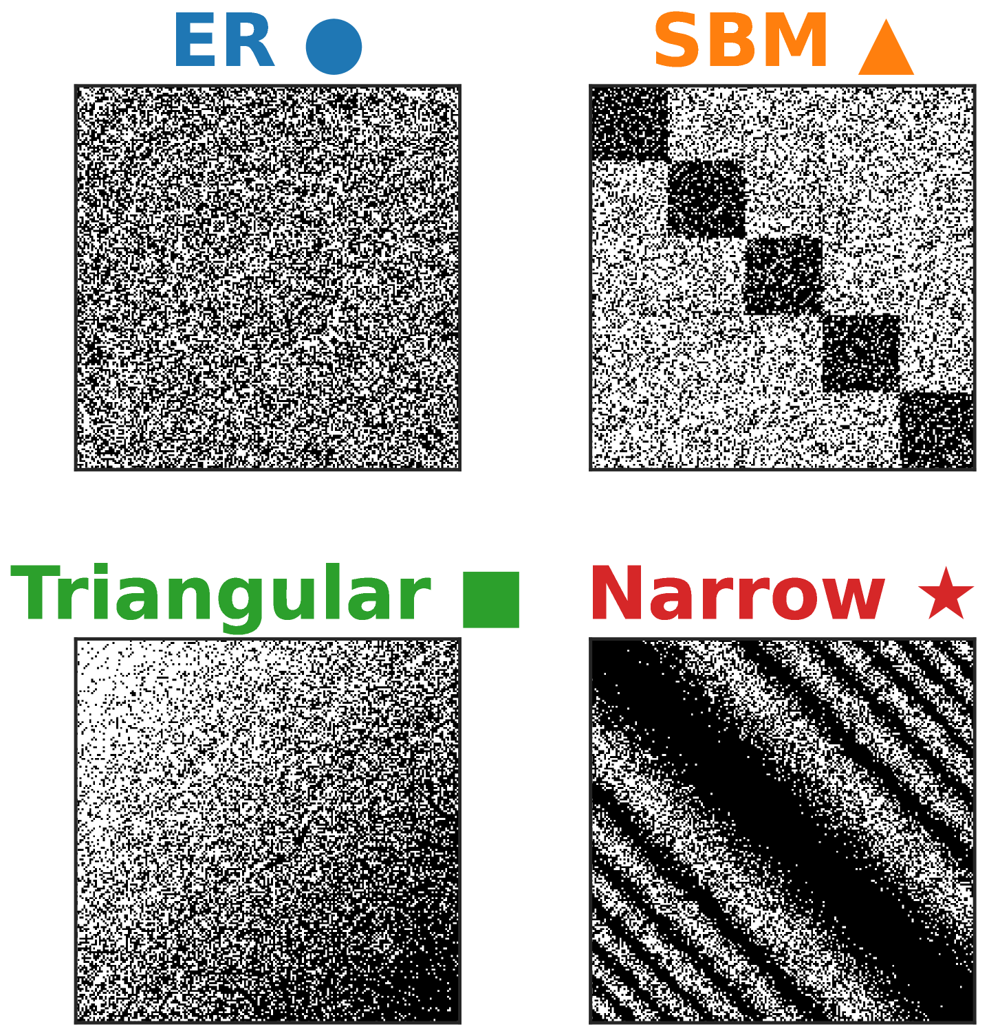
Figure 1: Example graphons $W$.

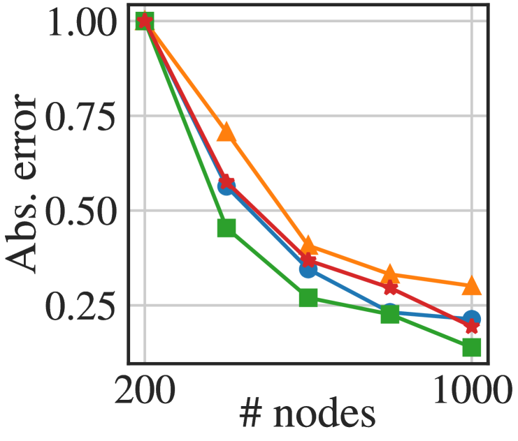
(a) MPNN

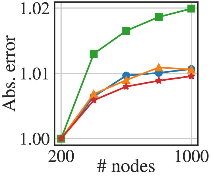
(b) 2-IWN

Figure 2: Absolute output errors $\mathcal{N}(W)$ vs. $\mathcal{N}(\mathbb{G}_{n}(W))$.

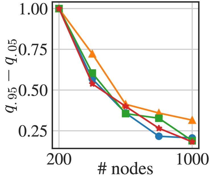
(a) MPNN

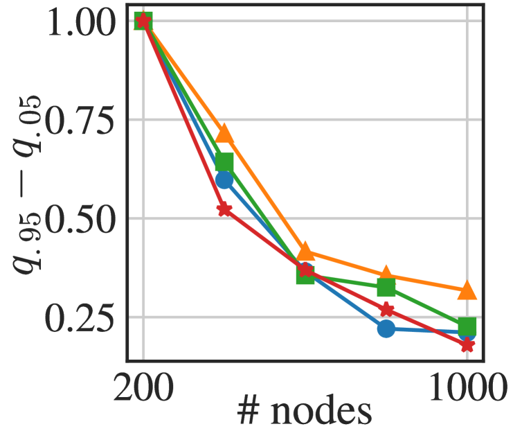
(b) 2-IWN

Figure 3: $90\%$ pred. interval widths of $\mathcal{N}(\mathbb{G}_{n}(W))$.

We also validate our theoretical findings for IWNs with a proof-of-concept experiment on the graphons from Figure 3. For continuity/convergence, we plot the absolute errors of the model outputs for the sampled simple graphs in comparison to their graphon limits in Figure 3. Due to the $\delta_{\square}$-continuity of MPNNs, their errors decrease as the graph size grows. For the IWN, however, this does not hold. Yet, the errors for the IWN stabilize with increasing sizes, suggesting that the outputs converge (just not to their graphon limit). For transferability, we further plot prediction interval widths of the output distributions on simple graphs for each of the sizes in Figure 3. Here, the widths contract for both models and there are only minor differences visible between the MPNN and the IWN. This validates Theorem 5.2 and suggests that IWNs have similar transferability properties as MPNNs. For more details, see Appendix H.

6 Conclusion

In this work, we study the continuity, expressivity, and transferability of graphon-based higher-order GNNs on the graphon-signal space (Levie, 2023) via signal-weighted homomorphism densities. We introduce Invariant Graphon Networks (IWNs) and analyze them through $L^{p}$ and cut distances on graphons. Significantly extending Cai & Wang (2022), we demonstrate that IWNs, as a subset of their IGN-small, retain the same expressive power as their discrete counterparts. Unlike MPNNs, IWNs are discontinuous w.r.t. cut distance, so standard transferability arguments (e.g., Ruiz et al. (2023); Levie (2023); Le & Jegelka (2024)) do not generalize. This stems from $k$-WL (Böker, 2023), so any $k$-WL expressive model on graphons has the same limitations. Yet, we show that this discontinuity can be overcome in the sense that higher-order GNNs are as transferable as MPNNs.

An intriguing avenue for future research could be developing more quantitative bounds on Theorem 5.2 under additional topological assumptions on the underlying graphon-signal. As our results make no such assumptions, the rate of convergence is essentially given by the graphon-signal sampling lemma. Furthermore, one could analyze expressive spectral methods (Lim et al., 2022; 2024; Huang et al., 2023). More broadly, future work could consider sparse graph limits (Le & Jegelka, 2024; Ruiz et al., 2024) or inductive biases through training, data distribution, or the specific task.

Acknowledgments

The authors would like to thank Thien Le, Manish Krishan Lal, and Levi Rauchwerger for insightful discussions at various stages of this work, and Andreas Bergmeister and Eduardo Santos Escriche for careful proofreading. This research was funded by an Alexander von Humboldt professorship.

Reproducibility Statement

We provide rigorous proofs of all our statements in the appendix, along with detailed explanations and the underlying assumptions. A comprehensive overview of our notation is listed in Appendix A. Details for the toy experiment are provided in Appendix H.

Appendices

[section] [section]l0

Appendix A Notation

Table 1: We list the most important symbols used in this work.

$\mathbb{N};\mathbb{N}_{0}$; $\mathbb{Q}$; $\mathbb{R}$	Natural, non-negative integer, rational, real numbers.
$[n]$	Set $\{1,\dots,n\}$ for $n\in\mathbb{N}$.
$\mathds{1}_{A}$	Indicator function of a set $A$.
$\{\cdot\}$	Explicit list of elements of a set.
$\{\!\!\{{\cdot}\}\!\!\}$	Explicit list of elements of a multiset.
$\varnothing$	Empty set and empty tuple.
$V(G);\;v(G)$	Node set of a graph; number of nodes of a graph $G$.
$E(G);\;e(G)$	Edge (multi)set of a (multi)graph; number of edges of a (multi)graph $G$.
$\deg(u)$	Degree of a node $u$ in a graph.
$\mathcal{O}(\cdot)$	“Big-O” notation for asymptotic growth of a function.
$o(\cdot)$	“Little-o” notation, indicating that the function is dominated by another.
$\mathcal{N}$	Generic variable for a neural network (MLP or GNN).
$\mathfrak{F}$	Generic variable for a function class of neural networks.
$\mathsf{tw}(F)$	Treewidth of a (multi)graph $F$.
$\mathsf{hom}(F,G)$	Number of homomorphisms from graph $F$ to $G$.
$\overline{A}$	Closure of a subset $A$ of a topological space $\mathcal{X}$.
$\mathcal{B}(\mathcal{X})$	Borel $\sigma$-algebra of a topological space $\mathcal{X}$.
$\sigma(\cdot)$	Generated $\sigma$-algebra.
$\mathbb{P}$	Probability measure.
$\mathbb{E}$	Expected value.
$\lambda;\lambda^{k}$	1-dimensional Lebesgue measure; $k$-dimensional Lebesgue measure.
$L^{p}(\mathcal{X})$	Space of $p$-integrable functions on a measure space $\mathcal{X}$, for $p\in[1,\infty]$.
$L^{p}_{r}(\mathcal{X})$	Space of $p$-integrable functions, with norm bounded by $r$.
$\left\|{\cdot}\right\|_{\square}$	Cut norm.
$\left\|{\cdot}\right\|_{p}$	$L^{p}$ norm of functions on a measure space, for $p\in[1,\infty]$.
$\left\|{\cdot}\right\|_{p,\mathcal{X}}$	$L^{p}$ norm, with emphasis on the underlying measure space $\mathcal{X}$.
$\mathcal{L}({V_{1}},{V_{2}})$	Space of bounded linear operators from normed vector space $V_{1}$ to $V_{2}$.
$\left\|{T}\right\|_{p\to q}$	Operator norm of $T\in\mathcal{L}({L^{p}(\mathcal{X})},{L^{q}(\mathcal{Y})})$.
$C(K)$	Space of continuous functions from compact topological space $K$ into $\mathbb{R}$, with uniform norm $\left\|{\cdot}\right\|_{\infty}$.
$\mathcal{W}$	Space of kernels.
$\mathcal{W}_{0}$	Space of graphons.
$\mathcal{WS}_{r}$	Space of graphon-signals $\mathcal{W}_{0}\times L^{\infty}_{r}[0,1]$.
$\widetilde{\mathcal{W}}_{0}$	Space of unlabeled graphons.
$\widetilde{\mathcal{WS}}_{r}$	Space of unlabeled graphon-signals.
$T_{W}$	Shift operator of a graphon $W$.
$S_{[0,1]}$	Measure preserving (almost) bijections of $[0,1]$.
$\overline{S}_{\mathcal{X}}$	Measure preserving functions $\mathcal{X}\to\mathcal{X}$, for a measure space $\mathcal{X}$.
$\delta_{\square}$	Cut distance.
$\delta_{p}$	$L^{p}$ distance for graphons/kernels.
$\delta_{N}$	Distance w.r.t. smooth invariant norms $N=(N_{1},N_{2})$.
$\overset{w}{\to}$	Weak convergence of probability measures.
$f_{\ast}\mu$	Pushforward of measure $\mu$ under $f$.
$W_{G}$	Step graphon of a graph $G$.
$\mathbb{H}_{k}(W)$; $\mathbb{H}_{k}(W,f)$	Distribution of weighted graphs/graph-signals of size $k$ sampled from a graphon $W$/graphon-signal $(W,f)$.
$\mathbb{G}_{k}(W)$; $\mathbb{G}_{k}(W,f)$	Distribution of unweighted graphs/graph-signals of size $k$ sampled from a graphon $W$/graphon-signal $(W,f)$.
$U(0,1)$	Uniform distribution on the interval $[0,1]$.
$t(F,W)$	Homomorphism density from a (multi)graph $F$ into graphon $W$.
$t((F,{\bm{d}}),(W,f))$	Signal-weighted homomorphism density from a (multi)graph $F$, ${\bm{d}}\in\mathbb{N}_{0}^{v(F)}$, into graphon-signal $(W,f)$.
${\bm{F}}=(F,{\bm{a}},{\bm{b}},{\bm{d}})$	Tri-labeled graph.
$\mathcal{M}^{k,\ell}$	Set of all tri-labeled graphs with $k$ input, $\ell$ output vertices.
${\bm{F}}_{1}\circ{\bm{F}}_{2}$	Composition of tri-labeled graphs.
${\bm{F}}_{1}\cdot{\bm{F}}_{2}$	Schur product of tri-labeled graphs.
$\mathcal{F}^{k}$	Set of atomic tri-labeled graphs.
$\langle\mathcal{F}\rangle$	Set of $\mathcal{F}$-terms.
$[\![\mathbb{F}]\!]$	Evaluation of a term $\mathbb{F}\in\langle\mathcal{F}\rangle$.
$h(\mathbb{F})$	Height of a term $\mathbb{F}$.
$T_{{\bm{F}}\to(W,f)}$	Graphon-signal operator associated with tri-labeled graph ${\bm{F}}$.
$\mathbb{M}^{k}_{s}$	Space of $k$-WL colors up to step $s$.
$\mathbb{M}^{k}$	Space of $k$-WL colors.
$p_{t\to s}$; $p_{\infty\to s}$	Canonical projections $\mathbb{M}_{t}^{k}\to\mathbb{M}_{s}^{k}$, $\mathbb{M}^{k}\to\mathbb{M}_{s}^{k}$.
$\mathbb{P}^{k}$	Space of $k$-WL refinements.
$F^{\mathbb{F}}$	Realizing functions on $\mathbb{M}^{k}$ of a term $\mathbb{F}$.
$t^{\mathbb{F}}$	Realizing function on $\mathbb{P}^{k}$ of a term $\mathbb{F}$.
$\mathfrak{C}_{(W,f)}^{k\text{-}\textnormal{WL},(s)}$	$k$-WL measure of $(W,f)\in\mathcal{WS}_{r}$.
$\nu_{(W,f)}^{k\text{-}\textnormal{WL}}$	$k$-WL distribution of $(W,f)\in\mathcal{WS}_{r}$.
$\textnormal{{LE}}^{\mathcal{X}}_{{k}\to{\ell}}$	Linear equivariant layers on measure space $\mathcal{X}$.
$\textnormal{{LE}}_{{k}\to{\ell}}$	Linear equivariant layers on $[0,1]$.
$\mathcal{F}_{k}^{(n)}$	Regular step functions in $L^{2}[0,1]^{k}$ at resolution $n$.
$\Gamma_{m}$	Set of partitions of $[m]$, $m\in\mathbb{N}_{0}$.
$\mathsf{bell}(m)$	$\left|{\Gamma_{m}}\right|$, i.e., number of partitions of $[m]$.
$\widetilde{\Gamma}_{k,\ell}$	Set of partitions of $[k+\ell]$ that index a basis of $\textnormal{{LE}}_{{k}\to{\ell}}$.
$T_{\gamma}$	Linear operator w.r.t. $\gamma\in\Gamma_{k+\ell}$.

Appendix B Extended Background

B.1 Topology and Measure Theory

We briefly recall fundamental definitions and results from topology, measure theory, and the theory of measures on Polish spaces that are used in this work. See, for example, Simon (2015) or Elstrodt (2018) for comprehensive primers.

B.1.1 Topology

A topological space is a pair $(\mathcal{X},\mathcal{O})$, where $\mathcal{X}$ is a set and the topology $\mathcal{O}\subseteq 2^{\mathcal{X}}$ is a collection satisfying that $\mathcal{X},\varnothing\in\mathcal{O}$, $\bigcup_{\iota\in I}U_{\iota}\in\mathcal{O}$ for any family $\{U_{\iota}\}_{\iota\in I}$ of $U_{\iota}\in\mathcal{O}$, and $U_{1}\cap\cdots\cap U_{n}\in\mathcal{O}$ for any $U_{1},\dots,U_{n}\in\mathcal{O}$. I.e., a topology is closed under arbitrary unions and finite intersections. A set $U\in\mathcal{O}$ is called open, and a set $A\in 2^{\mathcal{X}}$ is closed if its complement $A^{\mathsf{c}}:=\mathcal{X}\setminus A$ is open. The closure $\overline{A}$ of a set $A\subseteq\mathcal{X}$ is the smallest closed set containing $A$. A subset $A\subset\mathcal{X}$ is dense if its closure $\overline{A}=\mathcal{X}$. A topological space is separable if it has a countable dense subset. A neighborhood of $x\in\mathcal{X}$ is a set $A\subseteq\mathcal{X}$ such that there is an open set $U$ with $x\in U\subseteq A$. If the topology is clear from context, it is often left implicit.

A metric space is a pair $(\mathcal{X},d)$ with metric $d\colon\mathcal{X}\times\mathcal{X}\to[0,\infty)$ satisfying positive definiteness $d(x,y)=0$ iff $x=y$, symmetry $d(x,y)=d(y,x)$, and the triangle inequality $d(x,z)\leq d(x,y)+d(y,z)$ (here, $x,y,z\in\mathcal{X}$). A pseudometric is a function $d$ that satisfies all of the previous requirements except positive definiteness. A metric $d$ on $\mathcal{X}$ induces a topology by choosing the coarsest topology on $\mathcal{X}$ under which all balls $B_{\varepsilon}(x):=\{y\in\mathcal{X}|d(x,y)<\varepsilon\}$ for $x\in\mathcal{X}$, $\varepsilon>0$, are open. A topological space is metrizable if its topology can be induced by a metric. A topological space is Hausdorff if for any two points $x\neq y$ there exists a pair of disjoint neighborhoods. Metric spaces are trivially Hausdorff by positive definiteness. A metric space is complete if every Cauchy sequence in it converges to a point in the space. Note that this is a property of the metric itself and not of the induced topology. Spaces like $\mathbb{R}$ or $\mathbb{R}^{n}$ are typically considered with their standard topology, i.e. the one induced by the Euclidean norm/distance (which is the same for all norms).

A function $f\colon\mathcal{X}\to\mathcal{Y}$ between topological spaces $(\mathcal{X},\mathcal{O}_{\mathcal{X}})$ and $(\mathcal{Y},\mathcal{O}_{\mathcal{Y}})$ is continuous if for every open set $V\in\mathcal{O}_{\mathcal{Y}}$, one has $f^{-1}(V)\in\mathcal{O}_{\mathcal{X}}$. For metric spaces with their induced topology, this is equivalent to the standard definitions of continuity (via $\varepsilon$-$\delta$ or sequences).

An open cover of a topological space $\mathcal{X}$ is a family of open sets whose union is all of $\mathcal{X}$. A topological space $\mathcal{X}$ is compact if every open cover of $\mathcal{X}$ has a finite subcover; in metric spaces this is equivalent to every sequence in $\mathcal{X}$ having a convergent subsequence.

The product topology on $\prod_{\iota\in I}\mathcal{X}_{\iota}$ is the coarsest topology making all projections $p_{j}\colon\prod_{\iota\in I}\mathcal{X}_{\iota}\to X_{j}$ continuous, and if $A\subseteq\mathcal{X}$, the subspace topology on $A$ is $\{U\cap A\,|\,U\text{ open in }\mathcal{X}\}$. The convergence of a sequence in a topological product space is equivalent to convergence of all of its components, i.e., images under the projections $p_{\iota}$. A subset $A\subseteq\mathcal{X}$ is relatively compact if its closure is compact. By the Heine-Borel theorem, subsets of $\mathbb{R}^{n}$ are compact iff they are closed and bounded (in any norm).

A closed subset of a compact space is compact w.r.t. the subspace topology. The converse also holds if the space is Hausdorff. Tychonoff’s theorem states that any product $\prod_{\iota\in I}\mathcal{X}_{\iota}$ of compact topological spaces is again compact (regardless of the cardinality of $I$). A topological space is normal if any two disjoint closed subsets have disjoint open neighborhoods (i.e., open sets containing them). Every metrizable space is normal. The Tietze extension theorem states that if $\mathcal{X}$ is normal and $A\subseteq\mathcal{X}$ is closed, then any continuous function $f\colon A\to\mathbb{R}$ can be extended to a continuous function $\widetilde{f}\colon\mathcal{X}\to\mathbb{R}$.

Let $K$ be a compact Hausdorff space. Write $C(K,\mathbb{R})$ for the space of all continuous functions on $K$ (which are all bounded), equipped with the topology of uniform convergence, i.e., $\|{\cdot}\|_{\infty}$. With pointwise addition and multiplication, this space becomes an algebra. The Stone-Weierstrass theorem states that if $A\subset C(K,\mathbb{R})$ is a subalgebra that separates points in $K$ and contains the constant functions, then $A$ is dense in $C(K,\mathbb{R})$.

B.1.2 Measure Theory

A measurable space $(\mathcal{X},\mathcal{A})$ is a pair where $\mathcal{X}$ is an underlying set, and $\mathcal{A}\subseteq 2^{\mathcal{X}}$ is a $\sigma$-algebra, which fulfills $\varnothing\in\mathcal{A}$, and is stable under complements as well as countable unions. Note that this also implies stability under countable intersections. A measure space ($\mathcal{X},\mathcal{A}$, $\mu$) is a tuple, where $(\mathcal{X},\mathcal{A})$ is a measurable space and $\mu$ is a measure, i.e., a function from $\mathcal{A}$ to $[0,\infty]$ which satisfies $\mu(\varnothing)=0$, and $\sigma$-additivity $\mu(\bigcup_{n\in\mathbb{N}}A_{n})=\sum_{n\in\mathbb{N}}\mu(A_{n})$ for any disjoint $\{A_{n}\}_{n}\subseteq\mathcal{A}$. If the $\sigma$-algebra and/or measure is clear from context, we omit it. For any $\mathcal{G}\subseteq\mathcal{X}$, define its generated $\sigma$-algebra $\sigma(\mathcal{G})$ as the smallest $\sigma$-algebra containing $\mathcal{G}$ (this is well-defined as it is simply the intersection of all $\sigma$-algebras containing $\mathcal{G}$). A property of $\mathcal{X}$ holds almost everywhere (a.e.) if the set $N\in\mathcal{A}$ on which this property does not hold is a null set, i.e., $\mu(N)=0$. A probability space $(\mathcal{X},\mathcal{A},\mathbb{P})$ is a measure space with $\mathbb{P}(\mathcal{X})=1$.

The Borel $\sigma$-algebra $\mathcal{B}(\mathcal{X})$ on a topological space $\mathcal{X}$ is the $\sigma$-algebra generated by its open sets. Any continuous function on such a space is also measurable. The Lebesgue measure $\lambda$ on $\mathbb{R}$ is the unique measure on $\mathcal{B}(\mathbb{R})$ assigning intervals to its length. Analogously, $\lambda^{n}$ on $\mathcal{B}(\mathbb{R}^{n})$ is the unique measure assigning $n$-dimensional cuboids to its volume. These assignments determine the Lebesgue measure uniquely under translation invariance and regularity conditions. Often, the Lebesgue measure is considered on the Lebesgue $\sigma$-algebra, which is the completion of the Borel $\sigma$-algebra, containing all subsets of null sets. For this work, the distinction between both is not important, and we will work just with Borel sets. The counting measure on a set $\mathcal{X}$ is defined by mapping each subsets to its cardinality. Similarly to topologies, we can define subspace and product $\sigma$-algebras.

A function $f:(\mathcal{X},\mathcal{A}_{\mathcal{X}})\to(\mathcal{Y},\mathcal{A}_{\mathcal{Y}})$ between two measurable spaces is measurable if $f^{-1}(A)\in\mathcal{A}_{\mathcal{X}}$ for every $A\in\mathcal{A}_{\mathcal{Y}}$. The Lebesgue integral of a measurable function $f\colon(\mathcal{X},\mathcal{A},\mu)\to(\mathbb{R},\mathcal{B}(\mathbb{R}))$ is denoted by $\int_{\mathcal{X}}f\,\mathrm{d}\mu$, and is defined via taking a.e. limits of indicator and step functions.

A linear operator $T\colon(V,\|{\cdot}\|_{V})\to(W,\|{\cdot}\|_{W})$ between two normed spaces is bounded iff $T$ is continuous w.r.t. their induced metrics, which is equivalent to $\|T\|_{V\to W}:=\sup_{\|v\|_{V}=1}\|Tv\|_{W}<\infty$. For a measure space $(\mathcal{X},\mathcal{A},\mu)$ and $1\leq p<\infty$, its $L^{p}$ space is defined as $L^{p}\!\left(\mathcal{X}\right)=\{f\colon\mathcal{X}\to\mathbb{R}|\,f\text{ is measurable, }\|f\|_{p}=(\int_{\mathcal{X}}|f|^{p}\,\mathrm{d}\mu)^{1/p}<\infty\}$. $L^{\infty}(\mathcal{X})$ is defined via the essential supremum, $\|f\|_{\infty}=\operatorname*{ess\,sup}\,f:=\inf\{M\geq 0|\,|f(x)|\leq M\text{ a.e.}\}$. Functions that agree a.e. are identified.

In $L^{p}$ spaces, the following inequalities hold: Minkowski’s inequality states that $\|f+g\|_{p}\leq\|f\|_{p}+\|g\|_{p}$. Jensen’s inequality states that in a probability space $\mathcal{X}$ and for a convex function $\phi\colon\mathbb{R}\to\mathbb{R}$, $\phi\Bigl{(}\int_{\mathcal{X}}f\,d\mu\Bigr{)}\leq\int_{\mathcal{X}}\phi(f)\,\mathrm{d}\mu$. Hölder’s inequality states that for dual coefficients $p,q\in[1,\infty]$ with $1/p+1/q=1$, we have $\int_{\mathcal{X}}|fg|\,d\mu\leq\|f\|_{p}\|g\|_{q}$.

If $f\colon\mathcal{X}\to\mathcal{Y}$ is measurable and $\mu$ is a measure on $\mathcal{X}$, the pushforward measure $f_{\ast}\mu$ on $\mathcal{Y}$ is defined by $f_{\ast}\mu(A):=\mu\bigl{(}f^{-1}(A)\bigr{)}$ for all measurable $A\subseteq\mathcal{Y}$. If $g:\mathcal{Y}\to\mathbb{R}$ is measurable, then $\int_{\mathcal{Y}}g\,\mathrm{d}f_{\ast}\mu=\int_{\mathcal{X}}g\circ f\,\mathrm{d}\mu$ holds for the Lebesgue integral. A measure preserving function between two measure spaces $(\mathcal{X},\mu)$ and $(\mathcal{Y},\nu)$ is a measurable function $\varphi:\mathcal{X}\to\mathcal{Y}$ such that $\varphi_{\ast}\mu=\nu$. Two measure spaces $\mathcal{X}$ and $\mathcal{Y}$ are isomorphic if there exists a measure preserving bijection between them whose inverse is also measure preserving. The spaces are almost isomorphic if the former holds for some subsets of full measure of $\mathcal{X},\mathcal{Y}$.

B.1.3 Measures on Polish Spaces

A Polish space $\mathcal{X}$ is a topological space that is separable and completely metrizable, meaning that its topology is induced by a metric $d$ w.r.t. which $(\mathcal{X},d)$ is complete. We typically consider a Polish space with its Borel $\sigma$-algebra. A standard Borel probability space is a probability space defined on the Borel $\sigma$-algebra of a Polish space. Notably, by the isomorphism theorem, every nonatomic standard Borel probability space (meaning there are no points of positive measure) is almost isomorphic to the unit interval $([0,1],\mathcal{B}([0,1]),\lambda)$. By renormalization, a similar result holds for all finite measures.

Let $\mathcal{P}(\mathcal{X})$ be the set of all Borel probability measures on a Polish space $\mathcal{X}$. We equip this set with a topology as well: The weak topology of $\mathcal{P}(\mathcal{X})$ is the coarsest topology making all the maps $\mu\mapsto\int_{\mathcal{X}}f\,\mathrm{d}\mu$ continuous, where $f\in C_{b}(\mathcal{X})$ is considered over the bounded continuous functions on $\mathcal{X}$. This corresponds to the weak-$\ast$-topology on the dual $C_{b}(\mathcal{X})^{\ast}$, i.e., bounded linear functionals on $(C_{b}(\mathcal{X}),\|{\cdot}\|_{\infty})$. A sequence $(\mu_{n})_{n}$ of probability measures on $\mathcal{X}$ is said to converge weakly to $\mu$ (denoted $\mu_{n}\overset{w}{\to}\mu$) if $\int_{\mathcal{X}}f\,\mathrm{d}\mu_{n}\to\int_{\mathcal{X}}f\,\mathrm{d}\mu$ for every $f\in C_{b}(\mathcal{X})$.

The Portmanteau theorem gives several equivalent formulations of weak convergence (for example, convergence of the measures evaluated on continuity sets, or convergence of the integrals only for a dense subset of $C_{b}(\mathcal{X})$). On $\mathcal{X}=\mathbb{R}$, this is precisely convergence of random variables in distribution. Notably, if $\mathcal{X}$ is Polish, then so is $\mathcal{P}(\mathcal{X})$, and if $\mathcal{X}$ is metrizable and compact, this also carries over to $\mathcal{P}(\mathcal{X})$.

By Prokhorov’s theorem, a family of probability measures on a Polish space $\mathcal{X}$ is relatively compact (with respect to the weak topology) iff it is tight, meaning that the total probability mass can be approximated arbitrarily well by compact subsets $K_{\varepsilon}\subseteq\mathcal{X}$ uniformly on the family of measures.

B.2 Characterization of the IGN Basis

We restate the characterization of the IGN basis introduced by Cai & Wang (2022). As described by Maron et al. (2018), $\dim\textnormal{{LE}}^{[n]}_{{k}\to{\ell}}\,=\,\mathrm{bell}(k+\ell)$, i.e., the number of partitions $\Gamma_{k+\ell}$ of the set $[k+\ell]$. In the basis of Cai & Wang (2022), each basis element $L_{\gamma}^{(n)}$ associated with a partition $\gamma\in\Gamma_{k+\ell}$ can be characterized as a sequence of basic operations.

Given $\gamma\in\Gamma_{k+\ell}$, divide $\gamma$ into $3$ subsets $\gamma_{1}:=\{A\in\gamma\,|\,A\subseteq[k]\}$, $\gamma_{2}:=\{A\in\gamma\,|\,A\subseteq k+[\ell]\}$, $\gamma_{3}:=\gamma\setminus(\gamma_{1}\cup\gamma_{2})$. Here, the numbers $1,\dots,k$ are associated with the input axes and $k+1,\dots,k+\ell$ with the output axes respectively.

• (Selection: ${\bm{H}}\mapsto{\bm{H}}_{\gamma}$). In a first step, we specify which part of the input tensor ${\bm{H}}\in\mathbb{R}^{n^{k}}$ is under consideration. Take ${\left.\kern-1.2pt\gamma\vphantom{\big{|}}\right|_{[k]}}:=\{A\cap[k]\,|\,A\in\gamma,A\cap[k]\neq\varnothing\}$ and construct a new $|{\gamma_{1}}|+|{\gamma_{3}}|=|{{\left.\kern-1.2pt\gamma\vphantom{\big{|}}\right|_{[k]}}}|$-tensor ${\bm{H}}_{\gamma}$ by selecting the diagonal of the $k$-tensor ${\bm{H}}$ corresponding with the partition ${\left.\kern-1.2pt\gamma\vphantom{\big{|}}\right|_{[k]}}$.

• (Reduction: ${\bm{H}}_{\gamma}\mapsto{\bm{H}}_{\gamma,\textbf{red}}$). We average ${\bm{H}}_{\gamma}$ over the axes $\gamma_{1}\subseteq{\left.\kern-1.2pt\gamma\vphantom{\big{|}}\right|_{[k]}}$, resulting in a tensor ${\bm{H}}_{\gamma,\textbf{red}}$ of order $|{\gamma_{3}}|$, indexed by ${\left.\kern-1.2pt\gamma_{3}\vphantom{\big{|}}\right|_{[k]}}$.

• (Alignment: ${\bm{H}}_{\gamma,\textbf{red}}\mapsto{\bm{H}}_{\gamma,\textbf{align}}$). We align ${\bm{H}}_{\gamma,\textbf{red}}$ with a $|{\gamma_{3}}|$-tensor ${\bm{H}}_{\gamma,\textbf{align}}$ indexed by ${\left.\kern-1.2pt\gamma_{3}\vphantom{\big{|}}\right|_{k+[\ell]}}$, sending for $A\in\gamma_{3}$ the axis $A\cap[k]$ to $A\cap[\ell]$.

• (Replication: ${\bm{H}}_{\gamma,\textbf{align}}\mapsto{\bm{H}}_{\gamma,\textbf{rep}}$). Replicate the $|{\gamma_{3}}|$-tensor ${\bm{H}}_{\gamma,\textbf{align}}$ indexed by ${\left.\kern-1.2pt\gamma_{3}\vphantom{\big{|}}\right|_{k+[\ell]}}$ along the axes in $\gamma_{2}$. Note that if ${\left.\kern-1.2pt\gamma_{3}\vphantom{\big{|}}\right|_{k+[\ell]}}\cup\gamma_{2}$ contains non-singleton sets, the output tensor is supported on some diagonal.

Aggregations in this procedure can either be normalized (as described here) or simple sums. The basis element $T_{\gamma}^{(n)}:\mathbb{R}^{n^{k}}\to\mathbb{R}^{n^{\ell}}$ can now be described by the assignment $T_{\gamma}^{(n)}({\bm{H}}):={\bm{H}}_{\gamma,\textbf{rep}}$, and

$$\textnormal{{LE}}^{[n]}_{{k}\to{\ell}}\>=\>\mathrm{span}\left\{T^{(n)}_{\gamma}\,\middle|\,\gamma\in\Gamma_{k+\ell}\right\}.$$ (18)

B.3 IGN-small (Cai & Wang, 2022)

Cai & Wang (2022) study the convergence of discrete IGNs applied to graphs sampled from a graphon to a continuous version of the IGN defined on graphons. For this, they use the full IGN basis and a partition norm, which is for $U\in L^{2}[0,1]^{k}$ a $\mathsf{bell}(k)$-dimensional vector consisting of $L^{2}$ norms of $U$ on all possible diagonals. While they show that convergence of a discrete IGN on weighted graphs sampled from a graphon to its continuous counterpart holds, they also demonstrate that this is not the case for unweighted graphs with $\{0,1\}$-valued adjacency matrix.

As a remedy, Cai & Wang (2022) constrain the IGN space to IGN-small, which consists of IGNs for which applying the discrete version to a grid-sampled step graphon yields the same output as applying the continuous version and grid-sampling afterwards. In the following definition, we will formalize this. Here, $\mathcal{F}_{k}^{(n)}$ denotes the regular $k$-dimensional step kernels on $[0,1]$, $k\in\mathbb{N}_{0}$.

Definition B.1 (IGN-small (Cai & Wang, 2022)).

Let $\mathcal{N}$ be defined as in Definition 4.3, with the only difference that $\textnormal{{LE}}_{{k}\to{\ell}}$ is replaced by the full IGN basis, where averaging steps should be understood as integration. Cai & Wang (2022) call such $\mathcal{N}$ a continuous IGN. For any basis element $T_{\gamma}$, $\gamma\in\Gamma_{k+\ell}$, denote its discrete version at resolution $n\in\mathbb{N}$ by $T_{\gamma}^{(n)}$ and the network obtained by discretizing all equivariant linear layers by $\mathcal{N}^{(n)}$. Let

$$S^{(n)}:\mathbb{R}^{[0,1]^{k}\times d}\to\mathbb{R}^{n^{k}\times d},\;{\bm{U}}\mapsto(U(i/n,j/n))_{i,j=1}^{n}$$ (19)

be the grid-sampling operator. Then, $\mathcal{N}$ is contained in IGN-small if

$$(S^{(n)}\circ\mathcal{N})(W,f)\;=\;(\mathcal{N}^{(n)}\circ S^{(n)})(W,f)$$ (20)

for any $(W,f)\in\mathcal{WS}_{r}$ such that $W\in\mathcal{F}_{2}^{(n)}$, $f\in\mathcal{F}_{1}^{(n)}$. In this case, the input to such an IGN is $[(x,y)\mapsto(W(x,y),f(x))]$.

Cai & Wang (2022) show that convergence of IGN-small can be achieved in a model where a $\{0,1\}$-valued adjacency matrix is sampled from the graphon, provided that certain assumptions on the graphon and the signal—such as Lipschitz continuity—and a prior estimation of an edge probability are satisfied (see Theorem 4). It is important to note, however, that assuming the graphon is continuous is a rather strong condition, as it implies a topological structure on the node set corresponding to the unit interval. In contrast, similarly to Levie (2023), we treat $[0,1]$ solely as a measure space, which, being almost isomorphic to any nonatomic standard Borel probability space, is much more general. Regarding the expressivity of IGN-small, Cai & Wang (2022) establish that this model class can approximate spectral GNNs with arbitrary precision (cf. Theorem 5).

B.4 Tree Decomposition and Treewidth

In this section, we will recall the tree decomposition of a graph and the related notion of treewidth, which essentially captures how “far” a graph is from being a tree. See for example Diestel (2017, § 12.3) for a more in-depth discussion of this fundamental graph theoretic concept. We use the specific notation of Böker (2023).

Definition B.2 (Tree Decomposition of a Graph).

Let $G$ be a graph. A tree decomposition of $G$ is a pair $(T,\beta)$, where $T$ is a tree and $\beta:V(T)\to 2^{V(G)}$ such that

1. for every $v\in V(G)$, the set $\{t\,|\,v\in\beta(t)\}$ is nonempty and connected in $T$,

2. for every $e\in E(G)$, there is a node $t\in V(T)$ such that $e\subseteq\beta(t)$.

For $t\in V(T)$, the sets $\beta(t)\subseteq V(G)$ are commonly referred to as bags of the tree decomposition. Note that every graph $G$ has a trivial tree decomposition, given by a tree consisting of one node, with the bag being the entire node set $V(G)$. However, we are generally interested in finding tree decompositions with smaller bags. This leads us to the concept of treewidth:

Definition B.3 (Treewidth of a Graph).

Let $G$ be a graph. For any tree decomposition $(T,\beta)$ of $G$, define its width as

$$\max\{\left|{\beta(t)}\right|\,|\,t\in V(T)\}-1.$$ (21)

The treewidth of a graph $G$ is then the minimum width of all tree decompositions of $G$.

Note that, the edge graph of a tree $G$ can be seen as a tree decomposition of $G$, with each edge being a bag. Hence, the treewidth of a tree is 1. It can also be shown that, e.g., the treewidth of a circle of size at least 3 is 2. The definition can be extended to multigraphs by simply ignoring the edge multiplicities, i.e., considering the set of edges instead of the multiset.

B.5 Graphon-Signal Space (Levie, 2023)

Without reintroducing the graphon-signal space (see subsection 2.3 for the basic definitions), we formally restate two of the main results of Levie (2023) relevant to this work. Central to their contribution, Levie (2023) proves compactness of the graphon-signal space and provides a bound on its covering number. Note that something similar does not hold for any of the $\delta_{p}$ distances.

Theorem B.4 (Levie (2023), Theorem 3.6).

The space $(\widetilde{\mathcal{WS}}_{r},\delta_{\square})$ is compact. Moreover, given $r>0$ and $c>1$, for every sufficiently small $\varepsilon>0$, the space can be covered by $2^{k^{2}}$ balls of radius $\varepsilon$, where $k=\lceil 2^{\frac{9c}{4\varepsilon^{2}}}\rceil$.

The proof follows an approach analogous to that used for establishing the compactness of the space of unlabeled graphons and relies on a graphon-signal adaptation of the weak regularity lemma (Levie, 2023, Theorem B.6). The graphon-signal weak regularity lemma can also be used to derive a sampling lemma:

Theorem B.5 (Levie (2023), Theorem 3.7).

Let $r>1$. There exists a constant $N_{0}>0$ depending on $r$, such that for every $n\geq N_{0}$ and $(W,f)\in\mathcal{WS}_{r}$ we have

$$\mathbb{E}\left[\delta_{\square}\big{(}(W,f),\mathbb{G}_{n}(W,f)\big{)}\right]\,\leq\,\frac{15}{\sqrt{\log n}}.$$ (22)

Although the above results were obtained for one-dimensional signals, they readily extend to $d$-dimensional signals taking values in compact sets $K\subset\mathbb{R}^{d}$ (say, a hypercube $[-r,r]^{d}$) based on a multidimensional version of the signal cut norm normalized by $d$ (see Rauchwerger & Levie (2025) for a detailed treatment). In this case, the exact statements of Theorem B.4 and Theorem B.5 can be recovered. By norm equivalence, qualitative statements of the theorems remain valid when using the $L^{1}$ norm $\|{{\bm{f}}}\|_{1}$ as signal norm. The same reasoning extends to any $L^{1}$ norm defined from a vector norm $\|{\cdot}\|_{\mathbb{R}^{s}}$; that is, if one sets

$$\|{{\bm{f}}}\|:=\int_{[0,1]}\|{{\bm{f}}(x)}\|_{\mathbb{R}^{s}}\,\mathrm{d}\lambda(x),$$ (23)

as well as to other $L^{p}$ norms of ${\bm{f}}$: If for all signals ${\bm{f}}$, $x\mapsto\|{{\bm{f}}(x)}\|_{p}$ is uniformly bounded by $r$ on $[0,1]$, then

$$\int_{[0,1]}\|{{\bm{f}}(x)}\|_{p}\,\mathrm{d}\lambda(x)\>\leq\>\underbrace{\left(\int_{[0,1]}\|{{\bm{f}}(x)}\|_{p}^{p}\,\mathrm{d}\lambda(x)\right)^{1/p}}_{=\|{{\bm{f}}}\|_{p}}\>\leq\>r^{(p-1)/p}\left(\int_{[0,1]}\|{{\bm{f}}(x)}\|_{p}\,\mathrm{d}\lambda(x)\right)^{1/p},$$ (24)

where we used Jensen’s inequality for the first part.

Appendix C Signal-Weighted Homomorphism Densities

C.1 A Counting Lemma for Graphon-Signals

We derive a counting lemma similar to the standard graphon case (Lovász, 2012, Lemma 10.23), which shows that signal-weighted homomorphism densities from simple graphs into a graphon-signal are Lipschitz continuous w.r.t. cut distance.

Proposition C.1 (Counting lemma for graphon-signals).

Let $(W,f),(V,g)\in\mathcal{WS}_{r}$ and $F$ be a simple graph, ${\bm{d}}\in\mathbb{N}_{0}^{v(F)}$. Then, writing $D:=\sum_{i\in V(F)}d_{i}$,

$$\big{|}t((F,{\bm{d}}),(W,f))-t((F,{\bm{d}}),(V,g))\big{|}\;\leq\;2r^{D-1}\Big{(}2r\cdot e(F)\left\|{W-V}\right\|_{\square}+D\left\|{f-g}\right\|_{\square}\Big{)}.$$ (25)

As $t((F,{\bm{d}}),\cdot)$ is clearly invariant w.r.t. measure preserving functions acting on the graphon-signal, the bound of (25) can be easily extended to $\delta_{\square}$. The proof of Proposition C.1 is relatively straightforward, with the only detail requiring a little extra consideration being that the signals can take negative values and interact with the graphon. A similar statement can be shown for all multigraphs $F$ using $\left\|{\cdot}\right\|_{1}$.

Proof.

We split the l.h.s., bounding the difference of the graphons and the signals separately:

$$\big{|}t((F,{\bm{d}}),(W,f))-t((F,{\bm{d}}),(V,g))\big{|}\,\leq\,$$ (26)

$$\quad\underbrace{\left|{\int_{[0,1]^{k}}\left(\prod_{i\in V(F)}\!\!\!f(x_{i})^{d_{i}}\right)\left(\prod_{\{i,j\}\in E(F)}\!\!\!W(x_{i},x_{j})-\prod_{\{i,j\}\in E(F)}\!\!\!V(x_{i},x_{j})\right)\,\mathrm{d}\lambda^{k}({\bm{x}})}\right|}_{\leavevmode\hbox to7.49pt{\vbox to7.49pt{\text{[drawing]}}}}$$ (27)

$$+ \quad\underbrace{\left|{\int_{[0,1]^{k}}\left(\prod_{\{i,j\}\in E(F)}\!\!\!V(x_{i},x_{j})\right)\left(\prod_{i\in V(F)}\!\!\!f(x_{i})^{d_{i}}-\prod_{i\in V(F)}\!\!\!g(x_{i})^{d_{i}}\right)\,\mathrm{d}\lambda^{k}({\bm{x}})}\right|}_{\leavevmode\hbox to7.49pt{\vbox to7.49pt{\text{[drawing]}}}}.$$ (28)

For term , we set $D:=\sum_{i}d_{i}$ and observe that for all ${\bm{x}}\in[0,1]^{k}$

$$\frac{1}{r^{D}}\prod_{i\in V(F)}\!\!\!f(x_{i})^{d_{i}}\in[-1,1],\vskip-4.0pt$$ (29)

and hence similarly to the proof of the classical counting lemma (see, e.g., Zhao (2023)) we bound

$$\text{ \leavevmode\hbox to9.93pt{\vbox to9.93pt{\text{[drawing]}}}}\,\leq\,r^{D}e(F)\left\|{W-V}\right\|_{\square,2}\,\leq\,4r^{D}e(F)\left\|{W-V}\right\|_{\square}.$$ (30)

In comparison to the standard proof, the usage of $\left\|{\cdot}\right\|_{\square,2}$, an alternative definition of the cut norm, stems from the fact that function values appearing in the integral in (renormalizing by $r^{D}$) are not necessarily in $[0,1]$, but $[-1,1]$. See also equations (4.3), (4.4) in Janson (2013). For , we bound the $L^{1}$ difference of the terms involving $f$ and $g$:

$$\left|{\int_{[0,1]^{k}}\left(\prod_{\{i,j\}\in E(F)}\!\!\!V(x_{i},x_{j})\right)\left(\prod_{i\in V(F)}\!\!\!f(x_{i})^{d_{i}}-\prod_{i\in V(F)}\!\!\!g(x_{i})^{d_{i}}\right)\,\mathrm{d}\lambda^{k}({\bm{x}})}\right|$$ (31)

$$\leq\,\int_{[0,1]^{k}}\left|\prod_{\{i,j\}\in E(F)}\!\!\!V(x_{i},x_{j})\right|\left|\prod_{i\in V(F)}\!\!\!f(x_{i})^{d_{i}}-\prod_{i\in V(F)}\!\!\!g(x_{i})^{d_{i}}\right|\,\mathrm{d}\lambda^{k}({\bm{x}})$$ (32)

$$\leq\,\sum_{i\in V(F)}\int_{[0,1]^{k}}\Big{|}f(x_{i})^{d_{i}}-g(x_{i})^{d_{i}}\Big{|}\Big{|}\prod_{j<i}f(x_{j})^{d_{j}}\prod_{j>i}g(x_{j})^{d_{j}}\Big{|}\,\mathrm{d}\lambda^{k}({\bm{x}})$$ (33)

$$\leq\,\sum_{i\in V(F)}r^{\sum_{j\neq i}d_{i}}\int_{[0,1]}\left|f(x_{i})^{d_{i}}-g(x_{i})^{d_{i}}\right|\,\mathrm{d}\lambda(x)$$ (34)

$$\overset{(\ast)}{\leq}\,\sum_{i\in V(F)}r^{\sum_{j\neq i}d_{i}}\cdot d_{i}r^{d_{i}-1}\left\|{f-g}\right\|_{1}\,=\,Dr^{D-1}\left\|{f-g}\right\|_{1}\,\leq\,2Dr^{D-1}\left\|{f-g}\right\|_{\square},$$ (35)

where $(\ast)$ uses $\|{f}\|_{\infty},\|{g}\|_{\infty}\leq r$ and hence the Lipschitz constant of $x\mapsto x^{d_{i}}$ is bounded by the maximum of its derivative $d_{i}r^{d_{i}-1}$, and the last inequality uses $\left\|{\cdot}\right\|_{1}\leq 2\left\|{\cdot}\right\|_{\square}$ in one dimension. Combining the two bounds for from (30) and from (35), we obtain

$$\big{|}t((F,{\bm{d}}),(W,f))-t((F,{\bm{d}}),(V,g))\big{|}\,\leq\,4r^{D}e(F)\left\|{W-V}\right\|_{\square}+2Dr^{D-1}\left\|{f-g}\right\|_{\square},$$ (36)

which yields the claim. ∎

C.2 Smooth and Invariant Norms for Graphon-Signals

In this work, we consider not only the cut norm, but also $L^{p}$ norms (and distances) of graphon-signals. The purpose of this section is to show that all of the derived unlabeled distances we consider on the graphon-signal space yield the same notion of weak isomorphism, i.e., vanish simultaneously. This can be shown for smooth invariant norms on the graphon-signal space (cf. Lovász (2012, § 8.2.5)):

Definition C.2 (Smooth and invariant norms).

Two norms $N=(N_{1},N_{2})$, where $N_{1}$ is a norm on $L^{\infty}[0,1]$ and $N_{2}$ on $\mathcal{W}$, are called smooth if the two conditions

1. $W_{n}\to W\in\mathcal{W}$, $f_{n}\to f\in L^{\infty}[0,1]$ almost everywhere,

2. $\sup_{n\in\mathbb{N}}\|{W_{n}}\|_{\infty}\leq\infty$, $\sup_{n\in\mathbb{N}}\|{f_{n}}\|_{\infty}\leq\infty$,

imply that

$$N_{1}(f_{n})\to N_{1}(f),\qquad N_{2}(W_{n})\to N_{2}(W).$$ (37)

They are invariant if

$$N_{1}(f^{\varphi})=N_{1}(f),\quad N_{2}(W^{\varphi})=N_{2}(W)\qquad\forall\varphi\in S_{[0,1]},$$ (38)

where $(W,f)\in\mathcal{W}\times L^{\infty}[0,1]$ and $f^{\varphi}(x):=f(\varphi(x))$ for $x\in[0,1]$. We may sometimes also write $(W,f)^{\varphi}:=(W^{\varphi},f^{\varphi})$.

The conditions clearly apply to $\|{\cdot}\|_{\square}$ and $\|{\cdot}\|_{p}$ for $p\in[1,\infty)$ (acting either as $N_{1}$ and $N_{2}$), but do not hold for $p=\infty$ (take for example $W_{n}=\mathds{1}_{[0,1/n]^{2}}$, $f_{n}=\mathds{1}_{[0,1/n]}$). For any smooth and invariant $N$, we can obtain a derived unlabeled distance as done for the cut distance:

Definition C.3 (Derived unlabeled distance).

Let $N=(N_{1},N_{2})$ be smooth and invariant norms. Define its derived unlabeled distance on the graphon-signal space as

$$\delta_{N}((W,f),(V,g))\,:=\,\inf_{\varphi\in S_{[0,1]}}\big{(}N_{2}(W-V^{\varphi})+N_{1}(f-g^{\varphi})\big{)}.$$ (39)

Just as in the standard graphon case, for all such smooth and invariant norms, the infimum in (39) is attained when minimizing over all measure preserving functions. This turns out to be a generalization of Lovász (2012, Theorem 8.13):

Theorem C.4 (Minima vs. infima for smooth invariant norms).

Let $N$ be a smooth invariant norm on $\mathcal{W}$ and $L^{\infty}[0,1]$. Then, we have the following alternate expressions for $\delta_{N}$:

$$\delta_{N}((W,f),(V,g))\, =\,\inf_{\varphi\in\overline{S}_{[0,1]}}\big{(}N_{2}(W-V^{\varphi})+N_{1}(f-g^{\varphi})\big{)}$$ (40)

$$=\,\min_{\varphi,\psi\in\overline{S}_{[0,1]}}\big{(}N_{2}(W^{\varphi}-V^{\psi})+N_{1}(f^{\varphi}-g^{\psi})\big{)}.$$ (41)

Sketch of proof.

We follow the proof of Theorem 8.13 by Lovász (2012), briefly highlighting the necessary adjustments to the argument. To establish the first equality, approximations by step graphons that converge a.e. are considered, and the crucial point is that any $\varphi\in\overline{S}_{[0,1]}$ can be realized by a suitable $\widetilde{\varphi}\in S_{[0,1]}$ for such step graphons. For graphon-signals, the argument can be transferred if one simply considers partitions respecting each step graphon and step signal simultaneously when constructing the corresponding $\widetilde{\varphi}\in S_{[0,1]}$. For the second equality, which is proven in greater generality with coupling measures over $[0,1]^{2}$ by Lovász (2012), note that the lower semicontinuity in (8.24) is just shown for kernels (i.e., $L^{\infty}[0,1]^{2}$), but the argument extends verbatim to $L^{\infty}[0,1]$, and the sum of two lower semicontinuous functions is still lower semicontinuous. The rest of the argument applies without modification. ∎

Note that our definition of $\delta_{\square}$ coincides with the one by Levie (2023), as they also considered measure preserving bijections of co-null sets in $[0,1]$ (writing $S^{\prime}_{[0,1]}$ for this set). As an immediate corollary, we can obtain a simple characterization of weak isomorphism for graphon-signals:

Corollary C.5 (Weak isomorphism).

Two graphon-signals $(W,f),(V,g)\in\mathcal{WS}_{r}$ are weakly isomorphic, i.e., $\delta_{N}((W,f),(V,g))=0$ for any smooth and invariant norm $N=(N_{1},N_{2})$, if and only if there are $\varphi,\psi\in\overline{S}_{[0,1]}$ such that $W^{\varphi}=V^{\psi}$ and $f^{\varphi}=g^{\psi}$ almost surely.

Here, Theorem C.4 ensures that this does not depend on the specific $N$. Similar to standard graphons, we identify weakly isomorphic graphon-signals to obtain the space of unlabeled graphon-signals $\widetilde{\mathcal{WS}}_{r}$. We mainly work with the cut distance $\delta_{\square}$ as well as the $L^{p}$ distances $\delta_{p}$ for $p\in[1,\infty)$ (where we choose $N=(\|{\cdot}\|_{p},\|{\cdot}\|_{p}$)). Among these, of special interest are typically $\delta_{1}$ as this corresponds to the edit distance on graphs, as well as $\delta_{2}$, which gives rise to a geodesic space in the standard graphon case (Oh et al., 2024).

C.3 Proof of Theorem 3.2

See 3.2

The following elementary lemma will be useful on several occasions when comparing two probability distributions.

Lemma C.6 (Moments of Random Vectors).

Let $m\in\mathbb{N}$ and let ${\bm{X}},{\bm{Y}}$ be $m$-dimensional random vectors which are almost surely bounded, i.e., there is some $R>0$ such that $\mathbb{P}(\|{{\bm{X}}}\|\leq R)=\mathbb{P}(\|{{\bm{Y}}}\|\leq R)=1$, for any norm $\|{\cdot}\|$ on $\mathbb{R}^{m}$. Suppose that for all ${\bm{d}}\in\mathbb{N}_{0}^{m}$ the moments of ${\bm{X}},{\bm{Y}}$ agree:

$$\mathbb{E}\left[\prod_{i=1}^{m}X_{i}^{d_{i}}\right]\,=\,\mathbb{E}\left[\prod_{i=1}^{m}Y_{i}^{d_{i}}\right].$$ (42)

Then, ${\bm{X}}$ and ${\bm{Y}}$ are identically distributed, i.e., ${\bm{X}}\,\overset{\mathcal{D}}{=}\,{\bm{Y}}.$

Proof.

In the case of more general random variables/vectors, this is known in the literature as the moment problem (see, e.g., Schmüdgen (2017)). Under boundedness, however, this is trivial and can for example be proven via the characteristic functions of the random vectors. ∎

We are now ready to prove Theorem 3.2. To this end, we will show the implications in Figure 4.

Figure 4: Equivalence chain for the proof of Theorem 3.2.

Proof of Theorem 3.2.

(1) $\Leftrightarrow$ (2): Theorem C.4 implies that for any $p\in[1,\infty)$

$$\delta_{\square}((W,f),(V,g))=0\,\Leftrightarrow\,\exists\varphi,\psi\in\overline{S}_{[0,1]}:(W,f)^{\varphi}=(V,g)^{\psi}\,\Leftrightarrow\,\delta_{p}((W,f),(V,g))=0,$$ (43)

where equality in the middle holds in an $\lambda^{2}$-a.e. sense.

(2) $\Rightarrow$ (4): This follows immediately from Proposition C.1.

(4) $\Rightarrow$ (6): Let $(W,f),(V,g)\in\mathcal{WS}_{r}$ such that $t((F,{\bm{d}}),(W,f))=t((F,{\bm{d}}),(V,g))$ for all simple graphs $F$, ${\bm{d}}\in\mathbb{N}_{0}^{v(F)}$. Fix some $k\in\mathbb{N}$. Clearly, the distribution of $\mathbb{G}_{k}(W,f)$ is uniquely determined by

$$\mathbb{P}_{(G,{\bm{f}})\sim\mathbb{G}_{k}(W,f)}(G\cong F),$$ (44)

$$\mathbb{P}_{(G,{\bm{f}})\sim\mathbb{G}_{k}(W,f)}({\bm{f}}\in\cdot|G\cong F),$$ (45)

i.e., the discrete distribution of the (labeled) random graph $G$ and the conditional distribution of the node features given the graph structure, for every simple graph $F$ of size $k$. For (44), we remark that the standard homomorphism densities w.r.t. just the graphons $W,V$ can be recovered by taking ${\bm{d}}=0$. Thus, the inclusion-exclusion argument from the proof of Theorem 4.9.1 in (Zhao, 2023) can be used verbatim to reconstruct the probabilities from (44). With a similar inclusion-exclusion argument, we see that for any $F$

$$\mathds{1}\{\mathbb{G}_{k}(W)\cong F\}\,=\,\sum_{F^{\prime}\supseteq F}(-1)^{e(F^{\prime})-e(F)}\mathds{1}\{\mathbb{G}_{k}(W)\supseteq F^{\prime}\}$$ (46)

and therefore

$$\mathbb{E}_{(G,{\bm{f}})\sim\mathbb{G}_{k}(W,f)}\left[\prod_{i\in V(F)}f_{i}^{d_{i}}\middle|G\cong F\right]\,=\,\frac{\sum_{F^{\prime}\supseteq F}(-1)^{e(F^{\prime})-e(F)}\,t(F^{\prime},{\bm{d}},(W,f))}{\mathbb{P}_{(G,{\bm{f}})\sim\mathbb{G}_{k}(W,f)}(G\cong F)}$$ (47)

as long as the denominator is positive (otherwise, the corresponding conditional distribution is arbitrary). Since (${\bm{f}}|G\cong F$) is a bounded random vector ($\left\|{{\bm{f}}}\right\|_{\infty}\leq r$ a.s.), its distribution is uniquely determined by its multidimensional moments, i.e., precisely the expressions from (47) (see Lemma C.6). Thus, we can conclude $\mathbb{G}_{k}(W,f)\overset{\mathcal{D}}{=}\mathbb{G}_{k}(V,g)$ for all $k\in\mathbb{N}$.

(6) $\Rightarrow$ (2): This implication follows from applying the graphon-signal sampling lemma (Levie (2023, Theorem 3.7) and Theorem B.5): If (6) holds, we can bound

$$\delta_{\square}((W,f),(V,g))\, \leq\,\mathbb{E}\big{[}\delta_{\square}((W,f),\mathbb{G}_{k}(W,f))\big{]}+\mathbb{E}\big{[}\delta_{\square}((V,g),\mathbb{G}_{k}(W,f))\big{]}$$ (48)

$$=\,\mathbb{E}\big{[}\delta_{\square}((W,f),\mathbb{G}_{k}(W,f))\big{]}+\mathbb{E}\big{[}\delta_{\square}((V,g),\mathbb{G}_{k}(V,g))\big{]}\,\to\,0$$ (49)

as $k\to\infty$.

(1) $\Rightarrow$ (3): With a technique as in Proposition C.1, bounding the individual graphon terms in a similar way as the signal terms, it is straightforward to show that the signal-weighted homomorphism density $t((F,{\bm{d}}),\cdot)$ from any multigraph $F$ is also Lipschitz continuous w.r.t. $\delta_{1}$. Thus, statement (3) follows immediately.

(3) $\Rightarrow$ (5): Let $(W,f),(V,g)\in\mathcal{WS}_{r}$ such that $t((F,{\bm{d}}),(W,f))=t((F,{\bm{d}}),(V,g))$ for all multigraphs $F$, ${\bm{d}}\in\mathbb{N}_{0}^{v(F)}$. Fix $k\in\mathbb{N}$. Then, $\mathbb{H}_{k}(W,f)$ and $\mathbb{H}_{k}(V,g)$ can be seen as ($k^{2}+k$)-dimensional random vectors which are clearly bounded, since all graphon entries are in $[0,1]$ and all signal entries in $[-r,r]$. We observe that $\{t((F,{\bm{d}}),(W,f))\}_{F,{\bm{d}}}$ and $\{t((F,{\bm{d}}),(V,g))\}_{F,{\bm{d}}}$, with $F$ ranging over multigraphs of size $k$, are precisely the multidimensional moments of these random vectors. Lemma C.6 yields statement (5).

(5) $\Rightarrow$ (6): This is immediate, as $\mathbb{G}_{k}(\cdot)$ is a function of $\mathbb{H}_{k}(\cdot)$. ∎

C.4 Proof of Corollary 3.3

See 3.3

Proof.

The proof idea is essentially the same as in the classical graphon case (for example, see § 4.9 in Zhao (2023)): An application of Theorem 3.2 that uses compactness of the graphon-signal space. For the sake of completeness, we restate the argument.

“$\Rightarrow$” follows immediately from the counting lemma (Proposition C.1). For “$\Leftarrow$”, let $(W_{n},f_{n})_{n}$ be a sequence of graphon-signals that left-converges to $(W,f)\in\mathcal{WS}_{r}$. By compactness (Levie, 2023, Theorem 3.6), there exists a subsequence $(W_{n_{i}},f_{n_{i}})_{i}$ converging to some limit $(V,g)$ in cut distance. But then also all signal-weighted homomorphism densities of the subsequence converge, and hence

$$t(F,{\bm{d}},(W,f))\,=\,t(F,{\bm{d}},(V,g))\quad\forall F,{\bm{d}}\in\mathbb{N}_{0}^{v(F)}.$$ (50)

Theorem 3.2 yields $\delta_{\square}((W,f),(V,g))=0$, i.e., also $(W_{n},f_{n})\to(W,f)$ in cut distance. ∎

Appendix D $k$-WL for Graphon-Signals

In this section, we demonstrate that signal-weighted homomorphism densities also make sense on the granularity level of the $k$-WL hierarchy. Specifically, we show that their indistinguishability aligns with a natural formulation of the $k$-WL test for graphon-signals:

See 3.4

Recently, Böker (2023) established a characterization of the $k$-WL test for graphons, linking it to multigraph homomorphism densities w.r.t. patterns of bounded treewidth. Building on this, we introduce a natural generalization of the $k$-WL measure and distribution by Böker (2023) to graphon-signals and highlight that their homomorphism expressivity can be captured through signal-weighted homomorphism densities. This serves as the final step in demonstrating the suitability of this extension for our analyses. Since, compared to the discrete case, the formulation for graphons and graphon-signals is significantly more technical and relies heavily on measure theory, we directly state the graphon-signal versions of the concepts. Our goal in this section is not a fully detailed exposition, but rather to give intuition and highlight the key modifications required in the definitions and arguments of Böker (2023) to make them work for graphon-signals.

D.1 Tri-Labeled Graphs and Graphon-Signal Operators

To relate the $k$-WL measure to homomorphism densities on standard graphons, Böker (2023, § 3.1) introduces bi-labeled graphs to define a set of operators that generalize the single shift operator $T_{W}$ used by Grebík & Rocha (2022) for 1-WL. Using bi-labeled graphs, they define operations that generate all multigraphs of treewidth $\leq k-1$ by taking the closure of a set of atomic graphs under these operations. Intuitively, decomposing a bi-labeled graph into atomic parts corresponds to a tree decomposition with a certain special structure. This effectively allows one to express homomorphism densities via elementary operators associated with atomic graphs. This concept can be generalized to tri-labeled graphs for signal-weighted homomorphism densities:

Definition D.1 (Tri-labeled graphs).

A tri-labeled graph is a tuple ${\bm{G}}=(G,{\bm{a}},{\bm{b}},{\bm{d}})$, where $G$ is a multigraph, ${\bm{a}}\in V(G)^{k}$, ${\bm{b}}\in V(G)^{\ell}$ with $k,\ell\geq 0$, and ${\bm{d}}\in\mathbb{N}_{0}^{v(G)}$. Here, the entries of ${\bm{a}},{\bm{b}}$ each must be pairwise distinct. $(G,{\bm{d}})$ is called the underlying graph of ${\bm{G}}$, and ${\bm{a}},{\bm{b}}$ its input and output vertices. Write $\mathcal{M}^{k,\ell}$ for the set of all such graphs.

One can define some elementary operations with tri-labeled graphs: For ${\bm{F}}_{1}=(F_{1},{\bm{a}}_{1},{\bm{b}}_{1},{\bm{d}}_{1})\in\mathcal{M}^{k,\ell}$ and ${\bm{F}}_{2}=(F_{2},{\bm{a}}_{2},{\bm{b}}_{2},{\bm{d}}_{2})\in\mathcal{M}^{\ell,m}$, define the composition of ${\bm{F}}_{1}$ and ${\bm{F}}_{2}$ as

$${\bm{F}}_{1}\circ{\bm{F}}_{2}\>:=\>(F,{\bm{a}}_{1},{\bm{b}}_{2},{\bm{d}}_{1}+{\bm{d}}_{2})\>\in\>\mathcal{M}^{k,m},$$ (51)

where $F$ is obtained from $F_{1}\sqcup F_{2}$ by identifying the vertices in the tuples ${\bm{b}}_{1}$ and ${\bm{a}}_{2}$ (whose dimensions we required to be aligned), and the sum ${\bm{d}}_{1}+{\bm{d}}_{2}$ should be seen w.r.t. this identification. This identification also potentially introduces multiedges. The Schur product of ${\bm{F}}_{1}=(F_{1},{\bm{a}}_{1},\varnothing,{\bm{d}}_{1})$ and ${\bm{F}}_{2}=(F_{2},{\bm{a}}_{2},\varnothing,{\bm{d}}_{2})\in\mathcal{M}^{k,0}$ is defined as

$${\bm{F}}_{1}\cdot{\bm{F}}_{2}\>:=\>(F,{\bm{a}}_{1},\varnothing,{\bm{d}}_{1}+{\bm{d}}_{2})\>\in\>\mathcal{M}^{k,0},$$ (52)

where we abuse notation by writing $\varnothing$ for the empty tuple, and $F=F_{1}\sqcup F_{2}$, with the nodes in ${\bm{a}}_{1}$ and ${\bm{a}}_{2}$ identified. Now, also consider some atomic tri-labeled graphs which can be glued together using the above operations:

Definition D.2 (cf. Böker (2023, Definition 12)).

Let $k\geq 1$. Define the following specific tri-labeled graphs:

• Adjacency graph: ${\bm{A}}_{\{i,j\}}^{(k)}:=(([k],\{i,j\}),(1,\dots,k),(1,\dots,k),\bm{0})\in\mathcal{M}^{k,k}$ for $i\neq j$,

• Introduce graph: ${\bm{I}}_{j}^{(k)}:=(([k],\varnothing),(1,\dots,k),(1,\dots,j-1,j+1,\dots,k),\bm{0})\in\mathcal{M}^{k,k-1}$,

• Forget graph: ${\bm{F}}_{j}^{(k)}:=(([k],\varnothing),(1,\dots,j-1,j+1,\dots,k),(1,\dots,k),\bm{0})\in\mathcal{M}^{k-1,k}$,

• Neighbor graph: ${\bm{N}}_{j}^{(k)}:={\bm{I}}_{j}^{(k)}\circ{\bm{F}}_{j}^{(k)}\in\mathcal{M}^{k,k}$,

• Signal graph: ${\bm{S}}_{{\bm{d}}}^{(k)}:=(([k],\varnothing),(1,\dots,k),(1,\dots,k),{\bm{d}})\in\mathcal{M}^{k,k}$ for ${\bm{d}}\in\mathbb{N}_{0}^{k}$,

• All-one graph: $\bm{1}^{(k)}:=(([k],\varnothing),(1,\dots,k),\varnothing,\bm{0})\in\mathcal{M}^{k,0}$.

Define the set of all atomic tri-labeled graphs as   

$$\mathcal{F}^{k}\>:=\>\left\{{\bm{A}}_{\{i,j\}}^{(k)}\,\middle|\,i\neq j\in[k]\right\}\cup\left\{{\bm{N}}_{j}^{(k)}\,\middle|\,j\in[k]\right\}\cup\left\{{\bm{S}}_{{\bm{d}}}^{(k)}\,\middle|\,{\bm{d}}\in\mathbb{N}_{0}^{k}\right\}\>\subset\mathcal{M}^{k,k}.$$ (53)

These atomic graphs can now be joined by the elementary operations composition and Schur product to terms (Böker, 2023, Definition 13): For $k\geq 1$ and $\mathcal{F}\subseteq\mathcal{M}^{k,k}$, the set $\langle\mathcal{F}\rangle$ of $\mathcal{F}$-terms is the smallest set of expressions such that

$$\bm{1}^{(k)}\in\langle\mathcal{F}\rangle,$$ (54)

$${\bm{F}}\circ\mathbb{F}_{1}\in\langle\mathcal{F}\rangle \forall{\bm{F}}\in\mathcal{F},\mathbb{F}\in\langle\mathcal{F}\rangle,$$ (55)

$$\mathbb{F}_{1}\cdot\mathbb{F}_{2}\in\langle\mathcal{F}\rangle \forall\>\!\mathbb{F}_{1},\mathbb{F}_{2}\in\langle\mathcal{F}\rangle.$$ (56)

For such a term $\mathbb{F}$, write $[\![\mathbb{F}]\!]\in\mathcal{M}^{k,0}$ for its evaluation. Notably, Böker (2023, Definition 13) shows that the underlying graphs when evaluating the terms in their version of $\langle\mathcal{F}^{k}\rangle$ are precisely the multigraphs of treewidth bounded by $k-1$. In our case, we obtain

Theorem D.3 (cf. Böker (2023, Theorem 14)).

The underlying graphs of the tri-labeled graphs obtained by evaluating the terms in $\langle\mathcal{F}^{k}\rangle$ are precisely the node-featured multigraphs $(F,{\bm{d}})$ with $\mathsf{tw}(F)\leq k-1$, up to isolated vertices.

We omit the proof here; it is elementary and relies on the existence of certain nice tree decompositions (Kloks, 1994; Böker, 2023). In these (rooted) tree decompositions, roughly speaking, each edge where the bag changes corresponds to the addition or removal of a single node in a bag, and each bag has at most two children. Consequently, the tree can be traversed so that every edge is associated with one of the operations from Definition D.2.

Figure 5: A nice tree decomposition for a node-featured graph of treewidth 2, along with corresponding atomic tri-labeled graphs.

Consider, for example, the tri-labeled graph ${\bm{F}}=(F,{\bm{a}},\varnothing,{\bm{d}})\in\mathcal{M}^{3,0}$ from Figure 5 (the input vertices are highlighted), as well as a corresponding nice tree decomposition. ${\bm{F}}$ can be seen as the evaluation of the following term in $\mathcal{F}^{3}$:

$${\bm{F}}\>=\>{\color[rgb]{0,0.39453125,0.7421875}{\bm{S}}_{(d_{1},0,0)}^{(3)}}\circ\Big{(} \big{(}{\bm{A}}_{\{1,2\}}^{3}\circ{\bm{N}}_{3}^{(3)}\circ{\bm{A}}_{\{1,3\}}^{(3)}\circ{\bm{A}}_{\{2,3\}}^{(3)}\circ{\color[rgb]{0,0.39453125,0.7421875}{\bm{S}}_{(0,d_{2},d_{4})}^{(3)}}\circ\bm{1}^{(k)}\big{)}$$ (57)

$$\cdot \big{(}{\bm{A}}_{\{1,3\}}^{3}\circ{\bm{N}}_{2}^{(3)}\circ{\bm{A}}_{\{1,2\}}^{(3)}\circ{\bm{A}}_{\{2,3\}}^{(3)}\circ{\color[rgb]{0,0.39453125,0.7421875}{\bm{S}}_{(0,d_{5},d_{3})}^{(3)}}\circ\bm{1}^{(k)}\big{)}\Big{)}.$$ (58)

To later connect these terms in $\langle\mathcal{F}^{k}\rangle$ to the $k$-WL test, Böker (2023) defines the concept of height $h(\mathbb{F})$ for a term $\mathbb{F}$. Intuitively, this means that the homomorphism density w.r.t. the underlying graph of $[\![\mathbb{F}]\!]$ can be computed after $h(\mathbb{F})$ rounds of color refinement.

Definition D.4 (Height of a term).

We define the height $h(\mathbb{F})$ of a term $\mathbb{F}\in\langle\mathcal{F}^{k}\rangle$ inductively by setting $h(\bm{1}^{(k)}):=0$, $h({\bm{N}}\circ\mathbb{F}):=h(\mathbb{F})+1$ for any neighbor graph ${\bm{N}}$, $h({\bm{A}}\circ\mathbb{F}):=h(\mathbb{F})$ and $h({\bm{S}}\circ\mathbb{F}):=h(\mathbb{F})$ for any adjacency and signal graphs ${\bm{A}}$ and ${\bm{S}}$ respectively, and $h(\mathbb{F}_{1}\cdot\mathbb{F}_{2}):=\max\{h(\mathbb{F}_{1}),h(\mathbb{F}_{2})\}$.

We can define graphon-signal operators using tri-labeled graphs. Let ${\bm{F}}=(F,{\bm{a}},{\bm{b}},{\bm{d}})\in\mathcal{M}^{k,\ell}$ be a tri-labeled graph. Let $r>0$. Define the associated ${\bm{F}}$-operator of $(W,f)\in\mathcal{WS}_{r}$ as $T_{{\bm{F}}\to(W,f)}:L^{2}[0,1]^{\ell}\to L^{2}[0,1]^{k}$, which acts on $U\in L^{2}[0,1]^{\ell}$ as

$$\left(T_{{\bm{F}}\to(W,f)}U\right)({\bm{x}}_{\bm{a}})$$

$$\quad:=\int_{[0,1]^{v(F)-k}}\left(\prod_{i\in V(F)}f(x_{i})^{d_{i}}\right)\!\!\!\left(\prod_{\{i,j\}\in E(F)}\!\!\!\!\!\!W(x_{i},x_{j})\right)U({\bm{x}}_{\bm{b}})\,\mathrm{d}\lambda^{v(F)-k}({\bm{x}}_{V(F)\setminus{\bm{a}}}).$$ (59)

Importantly, composition (51) and Schur product (52) of tri-labeled graphs correspond to the composition and pointwise product of their associated operators, i.e.,

$$T_{{\bm{F}}_{1}\circ{\bm{F}}_{2}\to(W,f)}\> =\>T_{{\bm{F}}_{1}\to(W,f)}\circ T_{{\bm{F}}_{2}\to(W,f)} \forall{\bm{F}}_{1}\in\mathcal{M}^{k,m},\,{\bm{F}}_{2}\in\mathcal{M}^{m,\ell},\,k,l,m\geq 0,$$ (60)

$$T_{{\bm{F}}_{1}\cdot{\bm{F}}_{2}\to(W,f)}\> =\>T_{{\bm{F}}_{1}\to(W,f)}\cdot T_{{\bm{F}}_{2}\to(W,f)} \forall{\bm{F}}_{1},{\bm{F}}_{2}\in\mathcal{M}^{k,0},\,k\geq 0.$$ (61)

This allows us to gradually build up the operator $T_{[\![\mathbb{F}]\!]\to(W,f)}$ for any term $\mathbb{F}\in\langle\mathcal{F}^{k}\rangle$ from the operators w.r.t. its atomic graphs. It is also straightforward to see that just integrating over the output of such an operator applied to a constant function recovers the signal-weighted homomorphism densities. Formally, for any $(W,f)\in\mathcal{WS}_{r}$ and ${\bm{F}}=(F,{\bm{a}},{\bm{b}},{\bm{d}})\in\mathcal{M}^{k,\ell}$, we have

$$\int_{[0,1]^{k}}T_{{\bm{F}}\to(W,f)}\mathds{1}_{[0,1]^{\ell}}\,\mathrm{d}\lambda^{k}\>=\>t((F,{\bm{d}}),(W,f)).$$ (62)

D.2 Weisfeiler-Leman Measures

One can now define the space of colors used by the $k$-WL test for graphon-signals. In the discrete case—at least as long as node labels come from a countable alphabet—this space is countable and can be left implicit. However, for graphons and graphon-signals, the situation is more nuanced as the color space requires careful consideration of its topology, i.e., a suitable notion of convergence/distance.

Definition D.5 (Weisfeiler-Leman Measure, cf. Böker (2023, Definition 26)).

Let $k\geq 1$ and fix $r>0$. Let

$$P_{0}^{k}\>:=\>[0,1]^{[k]\choose 2}\times[-r,r]^{k}$$ (63)

be the space of initial colors. Inductively define

$$\mathbb{M}_{s}^{k}\>:=\>\prod_{i\leq s}P_{i}^{k},\qquad P_{s+1}^{k}\>:=\>\mathcal{P}(\mathbb{M}_{s}^{k})^{k}$$ (64)

for every $s\in\mathbb{N}$, where we consider $P_{0}^{k}$ with its standard topology, and $\mathcal{P}(\cdot)$ denotes the set of all Borel probability measures, equipped with the weak topology. Let $\mathbb{M}^{k}:=\prod_{s\in\mathbb{N}}P_{s}^{k}$ (equipped with the product topology) and define $p_{t\to s}:\mathbb{M}_{t}^{k}\to\mathbb{M}_{s}^{k}$ to be the natural projection for $s\leq t$. Set

$$\mathbb{P}^{k}\,:=\,\left\{\alpha\in\mathbb{M}^{k}\,|\,(\alpha_{s+1})_{j}\,=\,(p_{s+1\to s})_{\ast}(\alpha_{s+2})_{j}\text{ for all }j\in[k],s\in\mathbb{N}\right\},$$ (65)

where $(p_{s\to s+1})_{\ast}$ denotes the pushforward of measures.

We tacitly equip all spaces in Definition D.5 with their Borel $\sigma$-algebra. Intuitively, one can think of $\mathbb{P}^{k}$ as the space of all colors (potentially) used by the $k$-WL test, where for $\alpha\in\mathbb{P}^{k}$ each entry $\alpha_{s}$, $s\in\mathbb{N}$, is a refinement of the previous one. For any $\alpha\in\mathbb{P}^{k}$ and $j\in[k]$, there is a unique measure $\mu_{j}^{\alpha}\in\mathcal{P}(\mathbb{M}^{k})$ such that

$$(p_{\infty\to s})_{\ast}\mu_{j}^{\alpha}=(\alpha_{s+1})_{j},\qquad\forall s\in\mathbb{N},$$ (66)

by the Kolmogorov consistency theorem. A few basic statements about the topology of the spaces $\mathbb{M}^{k}$ and $\mathbb{P}^{k}$ are collected in the following lemma:

Lemma D.6 (cf. Böker (2023, p. 32 and Lemma 27)).

Consider $\mathbb{M}^{k}$ and $\mathbb{P}^{k}$ as in Definition D.5. The following holds:

1. The space $\mathbb{M}^{k}$ is metrizable and compact, and $\mathbb{P}^{k}\subseteq\mathbb{M}^{k}$ is closed.

2. The set

   $$\bigcup_{s\in\mathbb{N}_{0}}C(\mathbb{M}_{s}^{k})\circ p_{\infty\to s}\>\subset\>C(\mathbb{M}^{k})$$ (67)

   is dense.

3. For any $j\in[k]$, the assignment $\mathbb{P}^{k}\ni\alpha\mapsto\mu_{j}^{\alpha}\in\mathcal{P}(\mathbb{M}^{k})$ is continuous.

Proof.

Statement (1) follows immediately: $P_{0}^{k}$ is clearly metrizable and compact, and we can inductively conclude the same for $P_{s}^{k}$, $s\in\mathbb{N}$, as this is preserved by $\mathcal{P}(\cdot)$ and finite products. Also, as a countable product of metrizable and compact spaces, $\mathbb{M}^{k}$ is compact (by Tychonoff’s theorem) as well as metrizable. Now, let $\alpha^{(n)}\in\mathbb{P}^{k}$ such that $\alpha^{(n)}\to\alpha\in\mathbb{M}^{k}$. Clearly, for any $s\in\mathbb{N}$, $j\in[k]$, we have $(\alpha_{s+1}^{(n)})_{j}\overset{w}{\to}(\alpha_{s+1})_{j}$ by the definition of product topology, and for any $f\in C(\mathbb{M}^{k}_{s})$

$$\int_{\mathbb{M}^{k}_{s}}f\,\mathrm{d}(\alpha^{(n)}_{s+1})_{j}\,=\,\int_{\mathbb{M}^{k}_{s+1}}f\circ p_{s+1\to s}\,\mathrm{d}(\alpha_{s+2}^{(n)})_{j}\,\to\,\int_{\mathbb{M}^{k}_{s+1}}f\circ p_{s+1\to s}\,\mathrm{d}(\alpha_{s+2})_{j}\,=\,\int_{\mathbb{M}^{k}_{s}}f\,\mathrm{d}(\alpha_{s+1})_{j}$$ (68)

by the definition of the pushforward, and as $\alpha^{(n)}\in\mathbb{P}^{k}$. This implies also $(\alpha_{s+1}^{(n)})_{j}\overset{w}{\to}(p_{s+1\to s})_{\ast}(\alpha_{s+2})_{j}$, and, thus, $(\alpha_{s+1})_{j}=(p_{s+1\to s})_{\ast}(\alpha_{s+2})_{j}$ (as $\mathcal{P}(\mathbb{M}^{k}_{s})$ is metrizable and, hence, Hausdorff). We conclude $\alpha\in\mathbb{P}^{k}$, and $\mathbb{P}^{k}$ is closed. Particularly, this means that $\mathbb{P}^{k}$ is compact as well. For (2), note that the set is an algebra, clearly contains a constant function, and separates points of $\mathbb{M}^{k}$ (again, by the definition of product topology). The Stone-Weierstrass theorem yields the claim. Statement (3) follows similarly easily from (2). ∎

One can now define a set of “simple” functions on $\mathbb{M}^{k}$ which will turn out to be related to homomorphism densities. For a term $\mathbb{F}\in\langle\mathcal{F}^{k}\rangle$ of height $h(\mathbb{F})\leq s$, define a set of realizing functions $F^{\mathbb{F}}_{s}$ from $\mathbb{M}_{s}^{k}$ to $\mathbb{R}$ inductively as the smallest one fulfilling

$$F^{\bm{1}^{(k)}}_{s}\> \ni\>\mathds{1}_{\mathbb{M}_{s}^{k}},$$ (69)

$$F^{{\bm{A}}_{\{i,j\}}^{(k)}\circ\mathbb{F}}_{s}\> \ni\>\left[\alpha\mapsto((\alpha_{0})_{1})_{\{i,j\}}\cdot t(\alpha)\right] \forall t\in F^{\mathbb{F}}_{s},\,i\neq j\in[k],$$ (70)

$$F^{{\bm{S}}_{{\bm{d}}}^{(k)}\circ\mathbb{F}}_{s}\> \ni\>\left[\alpha\mapsto\prod_{i\in[k]}((\alpha_{0})_{2})_{i}^{d_{i}}\cdot t(\alpha)\right] \forall t\in F^{\mathbb{F}}_{s},\,{\bm{d}}\in\mathbb{N}_{0}^{k},$$ (71)

$$F^{{\bm{N}}_{j}^{k}\circ\mathbb{F}}_{s+1}\> \ni\>\left[\alpha\mapsto\int_{\mathbb{M}_{s}^{k}}t\,\mathrm{d}(\alpha_{s+1})_{j}\right] \forall t\in F^{\mathbb{F}}_{s},\,j\in[k],$$ (72)

$$F_{s}^{\mathbb{F}_{1}\cdot\mathbb{F}_{2}}\> \ni\>t_{1}\cdot t_{2} \forall t_{1}\in F_{s}^{\mathbb{F}_{1}},t_{2}\in F_{s}^{\mathbb{F}_{2}},$$ (73)

$$F_{s}^{\mathbb{F}}\> \ni\>t\circ p_{s\to t} \forall t\in F_{t}^{\mathbb{F}},t\leq s\leq h(\mathbb{F}).$$ (74)

Also, set

$$F^{\mathbb{F}}\>:=\>\bigcup_{s\in\mathbb{N}_{0}}\bigcup_{h(\mathbb{F})\leq s}F_{s}^{\mathbb{F}}\circ p_{\infty\to s}\;\subseteq\;L^{\infty}(\mathbb{M}^{k}).$$ (75)

One can check that each $t\in F^{\mathbb{F}}$ is continuous. By the consistency requirement on $\mathbb{P}^{k}$, the restriction of $F^{\mathbb{F}}$ to this subspace collapses to a singleton. Abusing notation, we define this realizing function of a term $\mathbb{F}\in\langle\mathcal{F}^{k}\rangle$ as

$$t^{\mathbb{F}}\>:=\>{\left.\kern-1.2ptF^{\mathbb{F}}\vphantom{\big{|}}\right|_{\mathbb{P}^{k}}}\>\in\>C(\mathbb{P}^{k}).$$ (76)

This leads to the following result:

Theorem D.7.

The sets

$$\mathrm{span}\bigcup_{\mathbb{F}\in\langle\mathcal{F}^{k}\rangle}F^{\mathbb{F}}\subset C(\mathbb{M}^{k})\qquad\text{and}\qquad\mathrm{span}\,\{t^{\mathbb{F}}\,|\,\mathbb{F}\in\mathcal{F}^{k}\}\subset C(\mathbb{P}^{k})$$ (77)

are dense w.r.t. $\|{\cdot}\|_{\infty}$.

The proof for $\mathbb{M}^{k}$ is tedious but conceptually simple, and relies on an inductive application of the Stone-Weierstrass theorem on $\mathbb{M}^{k}_{s}$ for $s\in\mathbb{N}$. Via Lemma D.6, (67), one can then arrive at $\mathbb{M}^{k}$ (this works, again, by a basic property of the product topology). The reader is referred to Böker (2023, Lemma 44) for the detailed argument. The statement for $\mathbb{P}^{k}$ follows immediately by its compactness.

D.3 Color Refinement for Graphon-Signals

One can now define the equivalent of the color refinement for a specific graphon-signal. Observe the close resemblance of the following definition to discrete $k$-WL test (cf. Huang & Villar (2021)).

Definition D.8 ($k$-WL, cf. Böker (2023, Definition 29)).

Let $k\geq 1$, $r>0$, and let $(W,f)\in\mathcal{WS}_{r}$. Define $\mathfrak{C}_{(W,f)}^{k\text{-}\textnormal{WL},(0)}:[0,1]^{k}\to\mathbb{M}_{0}^{k}$ by

$$\mathfrak{C}_{(W,f)}^{k\text{-}\textnormal{WL},(0)}({\bm{x}})\,:=\,\Big{(}\big{(}W(x_{i},x_{j})\big{)}_{\{i,j\}\in{[k]\choose 2}},\big{(}f(x_{j})\big{)}_{j\in[k]}\Big{)}\vskip-3.0pt$$ (78)

for every ${\bm{x}}\in[0,1]^{k}$. We then inductively define $\mathfrak{C}_{(W,f)}^{k\text{-}\textnormal{WL},(s+1)}\to\mathbb{M}_{s+1}^{k}$ by

$$\mathfrak{C}_{(W,f)}^{k\text{-}\textnormal{WL},(s)}({\bm{x}})\,:=\,\left(\mathfrak{C}_{(W,f)}^{k\text{-}\textnormal{WL},(s-1)}({\bm{x}}),\left(\left(\mathfrak{C}_{(W,f)}^{k\text{-}\textnormal{WL},(s-1)}\circ{\bm{x}}[\cdot/j]\right)_{\ast}\lambda\right)_{j\in[k]}\right)\vskip-3.0pt$$ (79)

for every ${\bm{x}}\in[0,1]^{k}$, where $\lambda$ is the Lebesgue measure and ${\bm{x}}[\cdot/j]:=(\dots,x_{j-1},\cdot,x_{j+1},\dots)\in[0,1]^{k}$. Let $\mathfrak{C}_{(W,f)}^{k\text{-}\textnormal{WL}}:[0,1]^{k}\to\mathbb{M}^{k}$ such that $(\mathfrak{C}_{(W,f)}^{k\text{-}\textnormal{WL}})_{s}=(\mathfrak{C}_{(W,f)}^{k\text{-}\textnormal{WL},(s)})_{s}$ for all $s\in\mathbb{N}$. Call

$$\nu_{(W,f)}^{k\text{-}\textnormal{WL}}\,:=\,\left(\mathfrak{C}_{(W,f)}^{k\text{-}\textnormal{WL}}\right)_{\ast}\lambda^{k}\,\in\,\mathcal{P}(\mathbb{M}^{k})$$ (80)

the $k$-dimensional Weisfeiler-Leman distribution of the graphon-signal $(W,f)$.

Intuitively, this corresponds with the multiset of colors that is obtained by the $k$-WL test for graphs. Consequentially, we call two graphon-signals $k$-WL-indistinguishable if and only if their $k$-WL distributions coincide. It is straightforward to show that $\nu_{(W,f)}^{k\text{-}\textnormal{WL}}(\mathbb{P}^{k})=1$, i.e., $k$-WL-distributions of graphon-signals indeed define color refinements in the sense of (65). Skipping all the technical details, we get directly to the homomorphism expressivity of this $k$-WL test. Notably, the realizing functions $t^{\mathbb{F}}$ of terms $\mathbb{F}\in\langle\mathcal{F}^{k}\rangle$ can be elegantly related to signal-weighted homomorphism densities via the terms from (76):

Proposition D.9 (cf. Böker (2023, Corollary 43)).

Let $k\geq 1$, $(W,f)\in\mathcal{WS}_{r}$, and $\mathbb{F}\in\langle\mathcal{F}^{k}\rangle$ with $[\![\mathbb{F}]\!]=(F,(1,\dots,k),\varnothing,{\bm{d}})\in\mathcal{M}^{k,0}$. Then, we have

$$t((F,{\bm{d}}),(W,f))\>=\>\int_{\mathbb{P}^{k}}t^{\mathbb{F}}\,\mathrm{d}\nu_{(W,f)}^{k\text{-}\textnormal{WL}}.$$ (81)

This leads to the following result, which generalizes Böker (2023, Theorem 5, (1) $\Leftrightarrow$ (2)):

Theorem D.10 ($k$-WL for graphon-signals, formal).

Let $r>0$ and $(W,f),(V,g)\in\mathcal{WS}_{r}$ be two graphon-signals. Then, $\nu_{(W,f)}^{k\text{-}\textnormal{WL}}=\nu_{(V,g)}^{k\text{-}\textnormal{WL}}$, i.e. the graphon-signals are $k$-WL indistinguishable, if and only if

$$t((F,{\bm{d}}),(W,f))\,=\,t((F,{\bm{d}}),(V,g))$$ (82)

for all multigraphs $F$ of treewidth $\leq k-1$ and ${\bm{d}}\in\mathbb{N}_{0}^{v(F)}$.

The arguments of Böker (2023) transfer almost verbatim to this setting. The crux is that in the $k$-WL test, both the distribution of the graphon values $W$ and the signal $f$ are captured already in the first step (78) and, therefore, higher-order moments need to be considered.

Appendix E Invariant Graphon Networks

E.1 Proof of Theorem 4.2

See 4.2

We will need some more preparations for the proof, in which we consider any $T\in\textnormal{{LE}}_{{k}\to{\ell}}$ only on step functions using regular intervals first, which will allow us to use the existing results for the discrete case.

Lemma E.1 (Fixed points of measure preserving functions).

If $k\in\mathbb{N}_{0}$ and $U\in L^{2}[0,1]^{k}$ such that $U^{\varphi}=U$ for all $\varphi\in\overline{S}_{[0,1]}$, then $U$ is constant. All involved equalities are meant $\lambda^{k}$-almost everywhere.

Although the proof is somewhat tedious, it is based on elementary measure theory. The aspect that warrants closer attention, however, is that $\varphi$ acts uniformly across all coordinates.

Proof.

Let $U\in L^{2}[0,1]^{k}$ such that $U$ is invariant under all measure preserving functions, and suppose that $U$ is not constant $\lambda^{k}$-almost everywhere. Then, there exist $a<b$ such that $A:=U^{-1}((-\infty,a])$, $B:=U^{-1}([b,\infty))$ have positive Lebesgue measure $\lambda^{k}(A),\lambda^{k}(B)>0$. Seeing $U$ as a random variable on the probability space $([0,1]^{k},\lambda^{k})$, the conditional distributions

$$\mathbb{P}(\cdot|U\leq a)\,=\,\frac{\lambda^{k}(\cdot\cap A)}{\lambda^{k}(A)}\quad\text{and}\quad\mathbb{P}(\cdot|U\geq b)\,=\,\frac{\lambda^{k}(\cdot\cap B)}{\lambda^{k}(B)}\vskip-2.0pt$$ (83)

are well-defined. For $n\in\mathbb{N}$, let $I_{j}^{(n)}:=[\frac{j-1}{n},\frac{j}{n})$ for $j\in\{1,\dots,n-1\}$ and $I_{n}^{(n)}:=[\frac{n-1}{n},1]$ be a partition of $[0,1]$ into regular intervals, and set $\mathcal{P}^{(n)}_{k}:=\{I_{j_{1}}^{(n)}\times\cdots\times I_{j_{k}}^{(n)}\,|\,j_{1},\dots,j_{k}\in\{1,\dots,n\}\}$. First, note that we have

$$\mathbb{P}(Q|U\leq a)\>\neq\>\mathbb{P}(Q|U\geq b)$$ (84)

for some $m\in\mathbb{N}$ and $Q\in\mathcal{P}^{(m)}_{k}$. Otherwise, equality in (84) would also hold for all hyperrectangles with rational endpoints, which is a $\cap$-stable generator of the Borel $\sigma$-algebra $\mathcal{B}([0,1]^{k})$. Consequently, equality would hold for all sets in $\mathcal{B}([0,1]^{k})$ and thus, $1=\mathbb{P}(A|U\leq a)=\mathbb{P}(A|U\geq b)=\lambda^{k}(\varnothing)/\lambda^{k}(B)=0$, which is a contradiction. W.l.o.g., assume $\mathbb{P}(Q|U\leq a)>\mathbb{P}(Q|U\geq b)$ in (84). As

$$\sum_{S\in\mathcal{P}^{(m)}_{k}}\mathbb{P}(S|U\leq a)\>=\>\sum_{S\in\mathcal{P}^{(m)}_{k}}\mathbb{P}(S|U\geq b)\>=\>1,$$ (85)

there must be another $R\in\mathcal{P}^{(m)}_{k}$ such that $\mathbb{P}(R|U\leq a)<\mathbb{P}(R|U\geq b)$. Set

$$\Delta_{k}\,:=\,\{{\bm{x}}\in[0,1]^{k}\,|\,\left|{\{x_{1},\dots,x_{k}\}}\right|<k\},\quad\Delta^{(n)}_{k}\,:=\,\{Q\in\mathcal{P}^{(n)}_{k}\,|\,Q\cap\Delta\neq\varnothing\}$$ (86)

to be the union of all diagonals on $[0,1]^{k}$ and the elements of $\mathcal{P}^{(n)}_{k}$ overlapping with $\Delta_{k}$ respectively for $n\in\mathbb{N}$. As $\lambda^{k}(\bigcup_{Q\in\Delta^{(n)}_{k}}Q)\to\lambda^{k}(\Delta_{k})=0$ as $n\to\infty$, there must exist $m^{\ast}\geq m\in\mathbb{N}$ such that there are $Q\supseteq Q^{\ast}\in\mathcal{P}^{(m^{\ast})}_{k}\setminus\Delta^{(m^{\ast})}_{k}$, $R\supseteq R^{\ast}\in\mathcal{P}^{(m^{\ast})}_{k}\setminus\Delta^{(m^{\ast})}_{k}$ satisfying

$$\mathbb{P}(Q^{\ast}|U\leq a)\>>\>\mathbb{P}(Q^{\ast}|U\geq b),\quad\mathbb{P}(R^{\ast}|U\leq a)\><\>\mathbb{P}(R^{\ast}|U\geq b).$$ (87)

Since $Q^{\ast}$ and $R^{\ast}$ do not overlap with any diagonal, we can now construct $\varphi\in S_{[0,1]}$ such that $\varphi^{\otimes k}$, which clearly defines a measure preserving function from $[0,1]^{k}$ to itself, sends $Q^{\ast}$ to $R^{\ast}$. By invariance of $U$ under all measure preserving functions, we get

$$\lambda^{k}(R^{\ast}\cap A)\, =\,\lambda^{k}\left((\varphi^{\otimes k})^{-1}(R^{\ast}\cap A)\right)\,=\,\lambda^{k}(Q^{\ast}\cap A),$$ (88)

$$\lambda^{k}(R^{\ast}\cap B)\, =\,\lambda^{k}\left((\varphi^{\otimes k})^{-1}(R^{\ast}\cap B)\right)\,=\,\lambda^{k}(Q^{\ast}\cap B),$$ (89)

which contradicts (87). Hence, $U$ must be $\lambda^{k}$-a.e. constant. ∎

Let $k,\ell\in\mathbb{N}_{0}$ and $n\in\mathbb{N}$. Let $I_{j}^{(n)}:=[\frac{j-1}{n},\frac{j}{n})$ for $j\in\{1,\dots,n-1\}$ and $I_{n}^{(n)}:=[\frac{n-1}{n},1]$ be a partition of $[0,1]$ into regular intervals. Let $\mathcal{A}_{n}:=\sigma\left(\{I_{1}^{(n)},\dots,I_{n}^{(n)}\}\right)$ denote the $\sigma$-algebra generated by this partition and let

$$\mathcal{F}_{k}^{(n)}:=\{U\in L^{2}[0,1]^{k}\,|\,U\text{ is }\mathcal{A}_{n}^{\otimes k}\text{-measurable}\};$$ (90)

define $\mathcal{F}_{\ell}^{(n)}$ similarly. Intuitively, this is just the set of regular $k$-dimensional $L^{2}$ step kernels.

Lemma E.2 (Invariance under discretization).

Any $T\in\textnormal{{LE}}_{{k}\to{\ell}}$ is invariant under discretization, which means that for any $n\in\mathbb{N}$, $T(\mathcal{F}_{k}^{(n)})\,\subseteq\,\mathcal{F}_{\ell}^{(n)}$, where the inclusion should be understood up to sets of measure zero.

Proof.

Let $T\in\textnormal{{LE}}_{{k}\to{\ell}}$ and let $U\in\mathcal{F}_{k}^{(n)}$. Then, if $\varphi\in\overline{S}_{[0,1]}$ such that

$$\varphi(I_{j}^{(n)})\subseteq I_{j}^{(n)}$$ (91)

for any $j\in\{1,\dots,n\}$, we have $U^{\varphi}=U$ and hence also $T(U)^{\varphi}=T(U)$ $\lambda^{\ell}$-almost everywhere. Take any hypercube $Q=I_{j_{1}}^{(n)}\times\dots\times I_{j_{\ell}}^{(n)}$ with $j_{1},\dots,j_{\ell}\in\{1,\dots,n\}$ and any measure-preserving function $\varphi:[0,1/n)\to[0,1/n)$. We replicate $\varphi$ on the unit interval as

$$\varphi^{\ast}(x)\,:=\,x\,\mathrm{div}\,1/n\;+\;\varphi\left(x\,\mathrm{mod}\,1/n\right),$$ (92)

which clearly satisfies (91), and thus $T(U)^{\varphi^{\ast}}=T(U)$ almost everywhere. Since now

$${\left.\kern-1.2ptT(U)\vphantom{\big{|}}\right|_{Q}}\,=\,{\left.\kern-1.2ptT(U)^{\varphi^{\ast}}\vphantom{\big{|}}\right|_{Q}}\,=\,\left({\left.\kern-1.2ptT(U)\vphantom{\big{|}}\right|_{Q}}\right)^{\varphi},$$ (93)

where we identify $\varphi$ with ${\left.\kern-1.2pt\varphi^{\ast}\vphantom{\big{|}}\right|_{I_{j}^{(n)}}}$ (which define measure preserving functions on $I_{j}^{(n)}$), we can use translation invariance and scale equivariance of the Lebesgue measure to conclude by Lemma E.1 that ${\left.\kern-1.2ptT(U)\vphantom{\big{|}}\right|_{Q}}$ is constant $\lambda^{\ell}$-almost everywhere. As $Q$ was chosen arbitrarily, this implies the statement of the lemma. ∎

Equipped with Lemma E.2, we are now ready to show that the dimension of linear equivariant layers in $[0,1]$ is finite. Central to the argument is the observation that we can consider the action of any $T\in\textnormal{{LE}}_{{k}\to{\ell}}$ on step functions, and apply the characterization from Maron et al. (2018) to a sequence of nested subspaces, which fixes the operator on the entire space $L^{2}[0,1]^{k}$.

Proof of Theorem 4.2.

Let $n\in\mathbb{N}$ and $T\in\textnormal{{LE}}_{{k}\to{\ell}}$. By Lemma E.2, we know that $T(\mathcal{F}_{k}^{(n)})\subseteq\mathcal{F}_{\ell}^{(n)}$. Since $\mathcal{F}_{k}^{(n)}\cong(\mathbb{R}^{n})^{\otimes k}\cong\mathbb{R}^{n^{k}}$, we can regard ${\left.\kern-1.2ptT\vphantom{\big{|}}\right|_{\mathcal{F}_{k}^{(n)}}}:\mathcal{F}_{k}^{(n)}\to\mathcal{F}_{\ell}^{(n)}$ as a linear operator $\mathbb{R}^{n^{k}}\to\mathbb{R}^{n^{\ell}}$. Taking for any $\sigma\in S_{n}$ a measure-preserving transformation $\varphi_{\sigma}\in S_{[0,1]}$ with $\varphi_{\sigma}(I_{j})=I_{\sigma(j)}$, we can see that ${\left.\kern-1.2ptT\vphantom{\big{|}}\right|_{\mathcal{F}_{k}^{(n)}}}$ is also permutation equivariant, and we can use the characterization of the basis elements from Cai & Wang (2022) (see subsection B.2).

Note that for any $n,m\in\mathbb{N}$ we have $\mathcal{F}_{k}^{(n)}\subseteq\mathcal{F}_{k}^{(nm)}$ and the canonical basis elements $\{T_{\gamma}\}_{\gamma\in\Gamma_{k+\ell}}$ under the identification $\mathcal{F}_{k}^{(n)}\cong\mathbb{R}^{n^{k}},\mathcal{F}_{k}^{(m)}\cong\mathbb{R}^{m^{k}}$ are compatible in the sense that

$${\left.\kern-1.2ptT_{\gamma}^{(nm)}\vphantom{\big{|}}\right|_{\mathcal{F}_{k}^{(n)}}}=T_{\gamma}^{(n)}.$$ (94)

Hence, the coefficients of ${\left.\kern-1.2ptT\vphantom{\big{|}}\right|_{\mathcal{F}_{k}^{(n)}}}$ w.r.t. the canonical basis $\{T_{\gamma}^{(n)}\}_{\gamma\in\Gamma_{k+\ell}}$ do not depend on the specific $n\in\mathbb{N}$. W.l.o.g., assume that $T$ restricted to some $\mathcal{F}_{k}^{(n)}$ is a canonical basis function $T_{\gamma^{\ast}}^{(n)}$ (where $\gamma^{\ast}\in\Gamma_{k+\ell}$ does not depend on $n$).

We now take a closer look at the partition $\gamma^{\ast}$ and its induced function $T_{\gamma^{\ast}}^{(n)}$ described by the steps Selection, Reduction, Alignment, and Replication. Partition $\gamma^{\ast}$ into the 3 subsets $\gamma^{\ast}_{1}:=\{A\in\gamma^{\ast}\,|\,A\subseteq[k]\}$, $\gamma^{\ast}_{2}:=\{A\in\gamma^{\ast}\,|\,A\subseteq k+[\ell]\}$, $\gamma^{\ast}_{3}:=\gamma^{\ast}\setminus(\gamma^{\ast}_{1}\cup\gamma^{\ast}_{2})$. For the constant $U\equiv 1\in\mathcal{F}_{k}^{(1)}\subseteq L^{2}[0,1]^{k}$, $T_{\gamma^{\ast}}^{(n)}(U)\neq 0$ must also be constant a.e. by compatibility with discretization, so the partition $\gamma^{\ast}$ cannot correspond to a basis function whose images are supported on a diagonal. This is precisely equivalent to $|{A\cap(k+[\ell])}|\leq 1$ for all $A\in\gamma^{\ast}$. Now suppose that the input only depends on a diagonal. Denoting the restriction of the constant $U\equiv 1$ to the diagonal under discretization of $[0,1]$ into $n$ pieces by $U_{\gamma^{\ast}}^{(n)}$,

$$T_{\gamma^{\ast}}^{(n)}(U_{\gamma^{\ast}}^{(n)})\,=\,T_{\gamma^{\ast}}^{(n)}(U)\,=\,T_{\gamma^{\ast}}^{(1)}(U)\,\neq\,0$$ (95)

is constant, but $\|{U_{\gamma^{\ast}}^{(n)}}\|_{2}\to 0$ for $n\to\infty$, which contradicts boundedness (i.e., continuity) of the operator $T\in\mathcal{L}({L^{2}[0,1]^{k}},{L^{2}[0,1]^{\ell}})$. Hence, $\gamma^{\ast}$ must correspond to a basis function for which the selection step is trivial, i.e., $|{A\cap[k]}|\leq 1$ for all $A\in\gamma^{\ast}$.

This leaves us with only the partitions $\gamma\in\Gamma_{k+\ell}$ whose sets $A\in\gamma$ contain at most one element from $[k]$ and $k+[\ell]$ respectively. In the following Lemma E.3 we will check that for all of these partitions, the Reduction/Alignment/Replication-procedure (with averaging in the sense of integration over $[0,1]$) indeed yields a valid operator $T_{\gamma}\in\mathcal{L}({L^{2}[0,1]^{k}},{L^{2}[0,1]^{\ell}})$ which agrees with $T_{\gamma}^{(n)}$ on $\mathcal{F}_{k}^{(n)}$.

If we can now show that $\bigcup_{n\in\mathbb{N}}\mathcal{F}_{k}^{(n)}\subseteq L^{2}[0,1]^{k}$ is dense w.r.t. $\|{\cdot}\|_{2}$, we can conclude that $T=T_{\gamma^{\ast}}$, as $T$ is continuous and agrees with $T_{\gamma^{\ast}}$ on a dense subset. However, this follows by a simple application of the martingale convergence theorem: Considering $[0,1]^{k}$ with Lebesgue measure $\lambda^{k}$ as a probability space and $U\in L^{2}[0,1]^{k}$ as a random variable, we have $\mathbb{E}[U|\mathcal{A}_{n}^{\otimes k}]\in\mathcal{F}_{k}^{(n)}$. Also, $\sigma\left(\bigcup_{n\in\mathbb{N}}\mathcal{A}_{n}^{\otimes k}\right)=\mathcal{B}([0,1]^{k})$ is the entire Borel $\sigma$-Algebra as $\mathcal{A}_{n}$ contains all intervals with rational endpoints, so $\mathbb{E}[U|\mathcal{A}_{n}^{\otimes k}]\to\mathbb{E}[U|\mathcal{B}([0,1]^{k})]=U$ in $L^{2}$.

Define now

$$\widetilde{\Gamma}_{k,\ell}\,:=\,\left\{\gamma\in\Gamma_{k+\ell}\,|\,\forall A\in\gamma:|{A\cap[k]}|\leq 1,|{A\cap k+[\ell]}|\leq 1\right\}.$$ (96)

It is straightforward to show that

$$\left|\widetilde{\Gamma}_{k,\ell}\right|\;=\,\sum_{s=0}^{\min\{k,\ell\}}s!{k\choose s}{\ell\choose s},$$ (97)

which can be seen as follows: Any partition on the l.h.s. can contain $s\in\{0,\dots,\min\{k,\ell\}\}$ sets of size 2. Fixing some $s$, any of these sets can only contain one element from $[k]$ and one from $k+[\ell]$. For the elements occuring in sets of size 2, there are ${k\choose s}{\ell\choose s}$ options, and there are $s!$ ways to match the $s$ selected elements in $[k]$ with the $s$ elements in $k+[\ell]$, leaving us with the formula on the right. This concludes the proof. ∎

Note the resemblance of the basis elements $T_{\gamma}$ (10) to the definition of graphon-signal operators from subsection D.1. Loosely speaking, all operators $T_{\gamma}$ are variants of (59), where the roles of ${\bm{a}}$ and ${\bm{b}}$ are switched, w.r.t. an empty graph $F$.

E.2 Continuity of Linear Equivariant Layers

We note that the choice $p=2$ in Definition 4.1 is somewhat arbitrary, and $T_{\gamma}$ can indeed be seen as an operator $L^{p}\to L^{p}$ for any $p\in[1,\infty]$, with $\|{T_{\gamma}}\|_{p\to p}=1$. The case case $p=2$ is technically still needed to complete the proof of Theorem 4.2.

Lemma E.3 (Continuity of Linear Equivariant Layers w.r.t. $\|{\cdot}\|_{p}$).

Fix $k,\ell\in\mathbb{N}_{0}$. Let $T\in\textnormal{{LE}}_{{k}\to{\ell}}$ and $p\in[1,\infty]$. Then, $T$ can also be regarded as a bounded linear operator $L^{p}[0,1]^{k}\to L^{p}[0,1]^{\ell}$. Furthermore, all of the canonical basis elements from the proof of Theorem 4.2 have operator norm $\|{T}\|_{p\to p}=1$.

Proof.

If suffices to show boundedness of all canonical basis elements. Just as in (10), take $\gamma\in\widetilde{\Gamma}_{k,\ell}$ containing $s$ sets of size 2 $\{i_{1},j_{1}\},\dots,\{i_{s},j_{s}\}$ with $i_{1},\dots,i_{s}\in[k]$, $j_{1},\dots,j_{s}\in k+[\ell]$, and set ${\bm{a}}=(i_{1},\dots,i_{s})$, ${\bm{b}}=(j_{1},\dots,j_{s})$. Write $T_{\gamma}$ as

$$T_{\gamma}(U)\,:=\,\left[[0,1]^{\ell}\ni{\bm{y}}\,\mapsto\,{\left.\kern-1.2pt\int_{[0,1]^{k-s}}\!\!\!\!U({\bm{x}}_{\bm{a}},{\bm{x}}_{[k]\setminus{\bm{a}}})\,\mathrm{d}\lambda^{k-s}({\bm{x}}_{[k]\setminus{\bm{a}}})\vphantom{\big{|}}\right|_{{\bm{x}}_{\bm{a}}={\bm{y}}_{{\bm{b}}-k}}}\right].$$ (98)

Consider at first $p<\infty$. Clearly, (98) is also well-defined for $U\in L^{p}[0,1]^{k}$ and

$$\|{T_{\gamma}(U)}\|_{p}^{p}\, =\,\int_{[0,1]^{\ell}}\left|{{\left.\kern-1.2pt\int_{[0,1]^{k-s}}\!\!\!\!U({\bm{x}}_{\bm{a}},{\bm{x}}_{[k]\setminus{\bm{a}}})\,\mathrm{d}\lambda^{k-s}({\bm{x}}_{[k]\setminus{\bm{a}}})\vphantom{\big{|}}\right|_{{\bm{x}}_{\bm{a}}={\bm{y}}_{{\bm{b}}-k}}}}\right|^{p}\mathrm{d}\lambda^{\ell}({\bm{y}})$$ (99)

$$\leq\,\int_{[0,1]^{\ell}}{\left.\kern-1.2pt\int_{[0,1]^{k-s}}\!\!\!\!\left|{U({\bm{x}}_{\bm{a}},{\bm{x}}_{[k]\setminus{\bm{a}}})}\right|^{p}\,\mathrm{d}\lambda^{k-s}({\bm{x}}_{[k]\setminus{\bm{a}}})\vphantom{\big{|}}\right|_{{\bm{x}}_{\bm{a}}={\bm{y}}_{{\bm{b}}-k}}}\mathrm{d}\lambda^{\ell}({\bm{y}})$$ (100)

$$=\,\int_{[0,1]^{s}}\int_{[0,1]^{k-s}}\!\!\!\!\left|{U({\bm{x}}_{\bm{a}},{\bm{x}}_{[k]\setminus{\bm{a}}})}\right|^{p}\,\mathrm{d}\lambda^{k-s}({\bm{x}}_{[k]\setminus{\bm{a}}})\,\mathrm{d}\lambda^{s}({\bm{x}}_{\bm{a}})\,=\,\|{U}\|_{p}^{p},$$ (101)

with Jensen’s inequality being applied in the second step. Note that equality holds, e.g., for $U\equiv 1$, so $\|{T_{\gamma}}\|_{p\to p}=1$. For $p=\infty$, we also see

$$\|{T_{\gamma}(U)}\|_{\infty}\, =\,\operatorname*{ess\,sup}_{{\bm{y}}\in[0,1]^{\ell}}\left|{{\left.\kern-1.2pt\int_{[0,1]^{k-s}}\!\!\!\!U({\bm{x}}_{\bm{a}},{\bm{x}}_{[k]\setminus{\bm{a}}})\,\mathrm{d}\lambda^{k-s}({\bm{x}}_{[k]\setminus{\bm{a}}})\vphantom{\big{|}}\right|_{{\bm{x}}_{\bm{a}}={\bm{y}}_{{\bm{b}}-k}}}}\right|$$ (102)

$$\leq\,\operatorname*{ess\,sup}_{{\bm{y}}\in[0,1]^{\ell}}{\left.\kern-1.2pt\int_{[0,1]^{k-s}}\underbrace{\left|{U({\bm{x}}_{\bm{a}},{\bm{x}}_{[k]\setminus{\bm{a}}})}\right|}_{\leq\|{U}\|_{\infty}\text{ a.e.}}\,\mathrm{d}\lambda^{k-s}({\bm{x}}_{[k]\setminus{\bm{a}}})\vphantom{\big{|}}\right|_{{\bm{x}}_{\bm{a}}={\bm{y}}_{{\bm{b}}-k}}}$$ (103)

$$\leq\|{U}\|_{\infty},$$ (104)

again with equality for $U\equiv 1$. ∎

E.3 Asymptotic Dimension of Linear Equivariant Layers

We briefly analyze the asymptotic differences in dimension between $\textnormal{{LE}}^{[n]}_{{k}\to{\ell}}$, the linear equivariant layer space of discrete IGNs, and $\textnormal{{LE}}_{{k}\to{\ell}}=\textnormal{{LE}}^{[0,1]}_{{k}\to{\ell}}$, of IWNs. Recall that

$$\dim\textnormal{{LE}}^{[n]}_{{k}\to{\ell}}\; =\;\mathsf{bell}(k+\ell),$$ (105)

$$\dim\textnormal{{LE}}^{[0,1]}_{{k}\to{\ell}}\; =\;\sum_{s=0}^{\min\{k,\ell\}}s!{k\choose s}{\ell\choose s}.$$ (106)

For a comparison of the dimensions for the first few pairs $(k,\ell)$, see Table 2.

Table 2: Dimensions of $\textnormal{{LE}}^{[n]}_{{k}\to{\ell}}$ and $\textnormal{{LE}}^{[0,1]}_{{k}\to{\ell}}$.

$\dim\textnormal{{LE}}^{[n]}_{{k}\to{\ell}}$ 0 1 2 3 4 0 1 1 2 5 15 1 1 2 5 15 52 2 2 5 15 52 203 3 5 15 52 203 877 4 15 52 203 877 4140

$\dim\textnormal{{LE}}^{[0,1]}_{{k}\to{\ell}}$ 0 1 2 3 4 0 1 1 1 1 1 1 1 2 3 4 5 2 1 3 7 13 21 3 1 4 13 34 73 4 1 5 21 73 209

The case of bounded $k$ or $\ell$.

Immediately visible from Table 2 is the vastly different behavior of the two expressions as long as one of the variables $k$, $\ell$ is bounded: In the discrete case, whenever $k\to\infty$ or $\ell\to\infty$, we have $\mathsf{bell}(k+\ell)\to\infty$ superexponentially. However, for the case of $[0,1]$, suppose w.l.o.g. that only $k\to\infty$ and $\ell=\mathcal{O}(1)$ remains constant. Then, the corresponding dimension growth is bounded by

$$\dim\textnormal{{LE}}^{[0,1]}_{{k}\to{\ell}}\;=\;\dim\textnormal{{LE}}^{[0,1]}_{{\ell}\to{k}}\;=\;\mathcal{O}(k^{\ell}),$$ (107)

as (106) is dominated by $\binom{k}{\ell}$ in this case.

The case of $k\sim\ell$.

We will now consider the worst case, i.e., when $k$ grows roughly as fast as $\ell$. For simplicity, assume $k=\ell$, and thus

$$\dim\textnormal{{LE}}^{[n]}_{{k}\to{k}}\;=\;\mathsf{bell}(2k),\quad\dim\textnormal{{LE}}^{[0,1]}_{{k}\to{k}}\>=\>\sum_{s=0}^{k}s!{k\choose s}^{2}.$$ (108)

The bell numbers grow superexponentially, as can be seen by one of its asymptotic formulas (e.g., refer to Weisstein (, Equation 19)):

$$\mathsf{bell}(n)\;\sim\;\frac{1}{\sqrt{n}}\left(\frac{n}{W(n)}\right)^{n+1/2}\exp\left(\frac{n}{W(n)}-n-1\right),$$ (109)

where $W$ denotes the Lambert W-function, i.e., the inverse of $x\mapsto x\exp(x)$, or a simpler characterization due to Grunwald & Serafin (2024, Proposition 4.7), which is not strictly asymptotically tight but suffices in our case:

$$\left(\frac{1}{e}\frac{n}{\log n}\right)^{n}\,\leq\,\mathsf{bell}(n)\,\leq\,\left(\frac{3}{4}\frac{n}{\log n}\right)^{n},$$ (110)

as long as $n\geq 2$. Therefore, the dimension of linear equivariant layers in the discrete case can be bounded as

$$\dim\textnormal{{LE}}^{[n]}_{{k}\to{k}}\,\geq\,\left(\frac{1}{e}\frac{2k}{\log 2k}\right)^{2k}.$$ (111)

We will now provide bounds on the dimension in the continuous case. First note that by only considering the last addend,

$$\dim\textnormal{{LE}}^{[0,1]}_{{k}\to{k}}\,\geq\,k!\,\geq\,\mathsf{bell}(k)$$ (112)

still grows superexponentially. A well-known bound on the factorial (see, e.g., Knuth (1997, § 1.2.5, Ex. 24)) is

$$\frac{n^{n}}{e^{n-1}}\,\leq\,n!\,\leq\,\frac{n^{n+1}}{e^{n-1}},$$ (113)

for $n\in\mathbb{N}$. For a rough upper bound on the dimension, we consider just an even tensor order $k$:

$$\dim\textnormal{{LE}}^{[0,1]}_{{k}\to{k}}\, =\,\sum_{s=0}^{k}s!{k\choose s}^{2}$$ (114)

$$\leq\,(k+1)k!\binom{k}{k/2}^{2}\,=\,(k+1)\frac{k!^{3}}{(k/2)!^{4}}$$ (115)

$$\!\!\!\!\!\!\overset{(\ref{eq:fact_bound})}{\leq}\,(k+1)\frac{k^{3k+3}}{e^{3k-3}}\frac{e^{2k-4}}{(k/2)^{2k}}\,=\,\frac{1}{e}(k+1)k^{3}\left(\frac{4}{e}k\right)^{k},$$ (116)

which still grows significantly slower than (111).

E.4 Proof of Proposition 4.4

See 4.4

Proof.

Let $\mathcal{N}^{\>\!\textsc{iwn}}$ be an IWN as in Definition 4.3. By invariance under discretization (Lemma E.2), we can see that any linear equivariant layer in $\mathcal{N}^{\>\!\textsc{iwn}}$ fulfills a basis representation stability condition, and under the identification $\mathcal{F}_{k}^{(n)}\cong\mathbb{R}^{n^{k}}$, which is captured by grid-sampling, this directly implies that grid-sampling commutes with application of the IWN and its discrete equivalent. ∎

E.5 Proof of Lemma 4.5

See 4.5

Proof of Lemma 4.5.

Let

$$\mathcal{N}^{\>\!{\textsc{iwn}}}\>=\>\mathfrak{T}^{(S)}\circ\varrho\circ\cdots\circ\varrho\circ\mathfrak{T}^{(1)}$$ (117)

be an IWN as in Definition 4.3. By Lemma E.3, each $T\in\textnormal{{LE}}_{{k}\to{\ell}}$ is Lipschitz continuous w.r.t. $\|{\cdot}\|_{p}$ on the respective input and output space, and this immediately carries over to all $\mathfrak{T}^{(s)}$, $s\in[S]$. Hence, it suffices to check that the pointwise application of the nonlinearity, i.e., $L^{p}[0,1]^{k}\ni U\mapsto\varrho(U)$, is Lipschitz continuous for every $k\in\mathbb{N}_{0}$, where $\varrho$ is applied elementwise. If $C_{\varrho}$ is the Lipschitz constant of $\varrho$, we have

$$\|{\varrho(U)-\varrho(W)}\|_{p}^{p}=\int_{[0,1]^{k}}\!\!\left|{\varrho(U)-\varrho(W)}\right|^{p}\,\mathrm{d}\lambda^{k}\leq\int_{[0,1]^{k}}\!\!C_{\varrho}^{p}\left|{U-W}\right|^{p}\,\mathrm{d}\lambda^{k}=C_{\varrho}^{p}\|{U-W}\|_{p}^{p},$$ (118)

for $p<\infty$, and the claim follows similarly for $\|{\cdot}\|_{\infty}$. ∎

E.6 Proof of Theorem 4.6

We show that IWNs can approximate signal-weighted homomorphism densities w.r.t. graphs of size up to their order. For this, we model the product in the homomorphism densities explicitly while tracking which linear equivariant layers are being used by the IWN. The final result then follows by using a tree decomposition.

See 4.6

To establish this result, we first show that IWNs can approximate signal-weighted homomorphism densities for graphs of size up to their order. To facilitate the final step of combining these approximations via a tree decomposition, we refrain from integrating over all nodes of the pattern graph immediately. Instead, we keep some labeled nodes to serve as connection points—akin to the construction of signal-weighted homomorphism densities from tri-labeled graphs in subsection D.1.

Lemma E.4.

Let $r>0$, $R>0$, $\varrho:\mathbb{R}\to\mathbb{R}$ Lipschitz continuous and non-polynomial, and $k>1$. Let ${\bm{F}}=(F,{\bm{a}},{\bm{b}},{\bm{d}})\in\mathcal{M}^{\ell,k}$ be a tri-labeled graph with $V(F)=[k]$ and $\ell\leq k$. Write $\iota_{k}$ for the function that embeds any $U\in L^{2}[0,1]^{m}$ for $m\leq k$ as a $k$-tensor $\iota_{k}(U):=[[0,1]^{k}\ni{\bm{x}}\to U(x_{1},\dots,x_{m})]$. Consider now the map $\Phi_{\bm{F}}$ that implements

$$\Phi_{{\bm{F}}}:\left(L^{2}[0,1]^{k}\right)^{\!3}\to\left(L^{2}[0,1]^{k}\right)^{\!3},\;\begin{bmatrix}\iota_{k}(W)\\ \iota_{k}(f)\\ U\end{bmatrix}\mapsto\begin{bmatrix}\iota_{k}(W)\\ \iota_{k}(f)\\ (\iota_{k}\circ T_{{\bm{F}}\to(W,f)})U\end{bmatrix}$$ (119)

for any $(W,f)\in\mathcal{WS}_{r}$ and $U\in L^{2}[0,1]^{k}$ (technically, this is only partially specified in the first two coordinates). Then, extending notation informally, for any $\varepsilon>0$, there exists a $k$-order EWN $\mathcal{N}^{\>\!{\textsc{ewn}}}_{{\bm{F}}}$ with nonlinearity $\varrho$ such that uniformly on $(W,f)\in\mathcal{WS}_{r}$ and $U\in L^{\infty}_{R}[0,1]^{k}$

$$\left\|{\Phi_{{\bm{F}}}(W,f,U)-\mathcal{N}^{\>\!{\textsc{ewn}}}_{{\bm{F}}}(W,f,U)}\right\|_{\infty,[0,1]^{k}}\>\leq\>\varepsilon.$$ (120)

For the proof, we model the product in the graphon-signal operators explicitly while tracking which linear equivariant layers are being used by the EWN.

We start with a few further preparations for the proofs. Namely, our main goal will be to show that if an EWN of a fixed order can approximate a set of functions, it can also approximate their product (Lemma E.6). First, we show how we can approximate the identity with an EWN:

Lemma E.5.

Let $k>1$ and $R>0$. Let $\varrho:\mathbb{R}\to\mathbb{R}$ be differentiable at least at one point with nonzero derivative. For any $\varepsilon>0$, there exist $T^{(1)}$, $T^{(2)}\in\textnormal{{LE}}_{{k}\to{k}}$ such that for $\mathcal{N}^{\>\!{\textsc{ewn}}}:=T^{(2)}\circ\varrho\circ T^{(1)}$ we have

$$\left\|{\mathcal{N}^{\>\!{\textsc{ewn}}}(U)-U}\right\|_{\infty,[0,1]^{k}}\>\leq\>\varepsilon$$ (121)

uniformly for all $U\in L^{\infty}_{R}[0,1]^{k}$.

Proof.

We simply approximate the identity function using the nonlinearity $\varrho$. Let $x_{0}\in\mathbb{R}$ be a point at which $\varrho$ is differentiable with $\varrho^{\prime}(x_{0})\neq 0$. Fix $\varepsilon>0$. There exists some constant $\delta>0$ such that $\left|{x}\right|\leq\delta$ implies

$$\left|{\varrho(x_{0}+x)-\varrho(x_{0})-\varrho^{\prime}(x_{0})x}\right|\,\leq\,\varepsilon\left|{x}\right|.$$ (122)

Set

$$\mathrm{id}_{\varrho}(x)\,:=\,\frac{R}{\delta\varrho^{\prime}(x_{0})}\left(\varrho\left(x_{0}+\frac{\delta}{R}x\right)-\varrho(x_{0})\right).$$ (123)

Then, for any $x\in[-R,R]$, $\left|{\frac{\delta}{R}x}\right|\leq\delta$ and hence

$$\left|{\mathrm{id}_{\varrho}(x)-x}\right|\, =\,\left|{\frac{R}{\delta\varrho^{\prime}(x_{0})}}\right|\left|{\varrho\left(x_{0}+\frac{\delta}{R}x\right)-\varrho(x_{0})-\varrho^{\prime}(x_{0})\frac{\delta}{R}x}\right|$$ (124)

$$\leq\,\left|{\frac{R}{\delta\varrho^{\prime}(x_{0})}}\right|\varepsilon\left|{\frac{\delta}{R}x}\right|\,\leq\,\frac{R}{\left|{\varrho^{\prime}(x_{0})}\right|}\varepsilon.$$ (125)

We can now simply set $\mathcal{N}^{\>\!{\textsc{ewn}}}:=\mathrm{id}_{\varrho}$, acting on the function values of an input independently. Hence, for any $U\in L^{\infty}_{R}[0,1]^{k}$, we get

$$\left\|{\mathcal{N}^{\>\!{\textsc{ewn}}}(U)-U}\right\|_{\infty,[0,1]^{k}}\>\leq\>\frac{R}{\left|{\varrho^{\prime}(x_{0})}\right|}\varepsilon$$ (126)

directly by (125). Since the r.h.s. can be made arbitrarily small, the proof is complete. ∎

Lemma E.6.

Let $k>1$ and $R>0$. Let $\mathcal{N}^{\>\!{\textsc{ewn}}}_{1}$, …, $\mathcal{N}^{\>\!{\textsc{ewn}}}_{m}$ be $m\in\mathbb{N}$ EWNs of order $k\in\mathbb{N}$ and Lipschitz continuous nonlinearity $\varrho$, each with constant orders of $k$, the same input dimension $d$, and output dimension of 1, i.e., returning a function $[0,1]^{k}\to\mathbb{R}$. Fix $\varepsilon>0$. Then, there exists an EWN ${\mathcal{N}^{\>\!{\textsc{ewn}}}}^{\ast}$ of order $k$, such that for all $U\in(L^{\infty}_{R}[0,1]^{k})^{d}$

$$\left\|{\prod_{\ell=1}^{m}\mathcal{N}^{\>\!{\textsc{ewn}}}_{\ell}(U)\,-\,{\mathcal{N}^{\>\!{\textsc{ewn}}}}^{\ast}(U)}\right\|_{\infty,[0,1]^{k}}\,\leq\,\varepsilon.$$ (127)

For the proof, we will draw inspiration from Keriven & Peyré (2019). However, a crucial difference to their proof is that we do not rely on modeling multiplication by increasing the tensor orders.

Proof.

We will exploit a property of $\cos$ that allows us to express products as sums. Namely, it is well-known that for $x_{1},\dots,x_{m}\in\mathbb{R}$ we have

$$\prod_{j=1}^{m}\cos(x_{j})\;=\;\frac{1}{2^{m}}\sum_{\sigma\in\{\pm 1\}^{m}}\cos\left(\sum_{j=1}^{m}\sigma_{j}x_{j}\right).$$ (128)

Fix $\varepsilon>0$. At first, we will describe how to approximate any $\mathcal{N}^{\>\!{\textsc{ewn}}}_{\ell}$ using $\cos$ as a nonlinearity. By the classical universal approximation theorem (see for example Pinkus (1999, Theorem 3.1)), we can approximate $\varrho:\mathbb{R}\to\mathbb{R}$ on compact sets arbitrarily well by a feedforward neural network $\varrho_{\cos}$ with one hidden layer, using the cosine function as nonlinearity. For all $\ell\in[m]$, the set of values of all intermediate computations in the evaluation of $\mathcal{N}^{\>\!{\textsc{ewn}}}_{\ell}(U)$ for $U\in(L^{\infty}_{R}[0,1]^{k})^{d}$ is bounded, and we define $M_{1}\in[0,\infty)$ to be the supremum of this set. Note that this means that $\varrho$ is only ever evaluated on the compact set $[-M_{1},M_{1}]$ in $\{\mathcal{N}^{\>\!{\textsc{ewn}}}_{\ell}\}_{\ell}$. We can see that replacing each occurence of $\varrho$ in $\mathcal{N}^{\textsc{ewn}}_{\ell}$ by $\varrho_{\cos}$ and absorbing the linear factors into the linear equivariant layers again yields valid EWNs. Call these EWNs $\mathcal{N}^{\textsc{ewn}}_{\ell,\cos}$, $\ell=1,\dots,m$. The underlying feedforward neural network $\varrho_{\cos}$ can now be chosen such that for all $\ell\in[m]$, $U\in(L^{\infty}_{R}[0,1]^{k})^{d}$

$$\left\|{\mathcal{N}^{\>\!{\textsc{ewn}}}_{\ell,\cos}(U)-\mathcal{N}^{\>\!{\textsc{ewn}}}_{\ell}(U)}\right\|_{\infty,[0,1]^{k}}\,\leq\,\varepsilon.$$ (129)

Note that each $\mathcal{N}^{\>\!{\textsc{ewn}}}_{\ell,\cos}$ might have different numbers of layers. Hence, we invoke Lemma E.5 to equalize the number of layers, and add one more layer of the identity. We obtain EWNs $\widetilde{\mathcal{N}^{\>\!{\textsc{ewn}}}_{\ell,\cos}}$ such that

$$\left\|{\mathrm{id}_{\cos}(\widetilde{\mathcal{N}^{\>\!{\textsc{ewn}}}_{\ell,\cos}}(U))-\mathcal{N}^{\>\!{\textsc{ewn}}}_{\ell,\cos}(U)}\right\|_{\infty,[0,1]^{k}}\,\leq\,\varepsilon$$ (130)

for all $U\in(L^{\infty}_{R}[0,1]^{k})^{d}$. Using (128) and setting $\mathrm{id}_{\cos}(x)=c\cdot\cos(ax+b)+d$ for some $a,b,c,d\in\mathbb{R}$, we can now write

$$\prod_{\ell=1}^{m}\mathrm{id}_{\cos}(\widetilde{\mathcal{N}^{\>\!{\textsc{ewn}}}_{\ell,\cos}}(U))\, =\,\prod_{\ell=1}^{m}\left(c\cdot\cos(a\cdot\widetilde{\mathcal{N}^{\>\!{\textsc{ewn}}}_{\ell,\cos}}(U)+b)+d\right)$$ (131)

$$=\,\sum_{A\subseteq[m]}c^{\left|{A}\right|}d^{m-\left|{A}\right|}\left(\prod_{\ell\in A}\cos(a\cdot\widetilde{\mathcal{N}^{\>\!{\textsc{ewn}}}_{\ell,\cos}}(U)+b)\right)$$ (132)

$$=\,\sum_{A\subseteq[m]}\frac{c^{\left|{A}\right|}d^{m-\left|{A}\right|}}{2^{\left|{A}\right|}}\sum_{\sigma\in\{\pm 1\}^{A}}\cos\underbrace{\left(\sum_{\ell\in A}\sigma_{\ell}(a\cdot\widetilde{\mathcal{N}^{\>\!{\textsc{ewn}}}_{\ell,\cos}}(U)+b)\right)}_{(\ast)},$$ (133)

which can be represented by an EWN of order $k$ and one layer more compared to $\{\widetilde{\mathcal{N}^{\>\!{\textsc{ewn}}}_{\ell,\cos}}\}_{\ell}$, stacking the expressions from ($\ast$), applying the nonlinearity $\cos$ and aggregating the outputs as determined by the weighted sum. Let

$$M_{2}\,:=\,\max_{\ell\in[m]}\sup_{U}\|{\mathcal{N}^{\>\!{\textsc{ewn}}}_{\ell}(U)}\|_{\infty,[0,1]^{k}}.$$ (134)

Since for any $U\in(L^{\infty}_{R}[0,1]^{k})^{d}$

$$\left\|{\prod_{\ell=1}^{m}\mathrm{id}_{\cos}(\widetilde{\mathcal{N}^{\>\!{\textsc{ewn}}}_{\ell,\cos}}(U))-\prod_{\ell=1}^{m}\mathcal{N}^{\>\!{\textsc{ewn}}}_{\ell}(U)}\right\|_{\infty,[0,1]^{k}}$$ (135)

$$\quad\leq\,\sum_{\ell=1}^{m}\left\|{\left(\prod_{i>\ell}\mathrm{id}_{\cos}(\widetilde{\mathcal{N}^{\>\!{\textsc{ewn}}}_{\ell,\cos}}(U))\prod_{i<\ell}\mathcal{N}^{\>\!{\textsc{ewn}}}_{\ell}(U)\right)\left(\mathrm{id}_{\cos}(\widetilde{\mathcal{N}^{\>\!{\textsc{ewn}}}_{\ell,\cos}}(U))-\mathcal{N}^{\>\!{\textsc{ewn}}}_{\ell}(U)\right)}\right\|_{\infty,[0,1]^{k}}$$ (136)

$$\quad\leq\,\sum_{\ell=1}^{m}\left\|{\prod_{i>\ell}\mathrm{id}_{\cos}(\widetilde{\mathcal{N}^{\>\!{\textsc{ewn}}}_{\ell,\cos}}(U))\prod_{i<\ell}\mathcal{N}^{\>\!{\textsc{ewn}}}_{\ell}(U)}\right\|_{\infty,[0,1]^{k}}\left\|{\mathrm{id}_{\cos}(\widetilde{\mathcal{N}^{\>\!{\textsc{ewn}}}_{\ell,\cos}}(U))-\mathcal{N}^{\>\!{\textsc{ewn}}}_{\ell}(U)}\right\|_{\infty,[0,1]^{k}}$$ (137)

$$\quad\leq\,\sum_{\ell=1}^{m}(M_{2}+2\varepsilon)^{m-\ell}M_{2}^{\ell-1}2\varepsilon,$$ (138)

and since (138) goes to zero as $\varepsilon\to 0$, this shows the claim for $\cos$. Another application of the universal approximation theorem yields the claim for $\varrho$. ∎

The proof of Lemma E.4 now boils down to an application of Lemma E.6.

Proof of Lemma E.4.

Fix a tri-labeled graph ${\bm{F}}=(F,{\bm{a}},{\bm{b}},{\bm{d}})$ with $V(F)=[k]$, ${\bm{a}}$ and ${\bm{b}}$ $\ell$- and $k$-tuples over $[k]$ respectively. Let $(W,f)\in\mathcal{WS}_{r}$ and $U\in L^{\infty}_{R}[0,1]^{k}$. Define

$$f_{i}: [0,1]^{k}\to\mathbb{R},\;{\bm{x}}\mapsto f(x_{i})\qquad\qquad\text{for }i\in V(F),$$ (139)

$$W_{\{i,j\}}: [0,1]^{k}\to\mathbb{R},\;{\bm{x}}\mapsto W(x_{i},x_{j})\qquad\text{for }\{i,j\}\in E(F).$$ (140)

Clearly, $[\iota_{k}(W),\iota_{k}(f),U]^{\top}\mapsto f_{i}$, $[\iota_{k}(W),\iota_{k}(f),U]^{\top}\mapsto W_{\{i,j\}}$, and $[\iota_{k}(W),\iota_{k}(f),U]^{\top}\mapsto U_{\bm{b}}:=[{\bm{x}}\mapsto U({\bm{x}}_{\bm{b}})]$ can be exactly represented by EWNs of order $k$ with one layer (i.e., no application of the nonlinearity at all). By Lemma E.6, the product

$$\begin{bmatrix}\iota_{k}(W)\\ \iota_{k}(f)\\ U\end{bmatrix}\,\mapsto\,\left(\prod_{i\in V(F)}f_{i}^{d_{i}}\right)\left(\prod_{\{i,j\}\in E(F)}W_{\{i,j\}}\right)U_{\bm{b}}$$ (141)

can be approximated by an EWN of order $k$ arbitrarily well in $\|{\cdot}\|_{\infty}$. However, setting $D:=\sum_{i}d_{i}$,

$$T_{{\bm{F}}\to(W,f)}U\>=\>\int_{[0,1]^{k-\ell}}\left(\prod_{i\in V(F)}f_{i}^{d_{i}}\right)\left(\prod_{\{i,j\}\in E(F)}W_{\{i,j\}}\right)U_{\bm{b}}\,\mathrm{d}\lambda^{[k]\setminus{\bm{a}}}\>\in\>L^{\infty}_{Rr^{D}}[0,1]^{\ell},$$ (142)

and combined with applying Lemma E.5 again on $W$ and $f$, one concludes that

$$\begin{bmatrix}\iota_{k}(W)\\ \iota_{k}(f)\\ U\end{bmatrix}\mapsto\begin{bmatrix}\iota_{k}(W)\\ \iota_{k}(f)\\ (\iota_{k}\circ T_{{\bm{F}}\to(W,f)})U\end{bmatrix}$$ (143)

can be approximated arbitrarily well by an EWN for $(W,f)\in\mathcal{WS}_{r}$ and $U\in L^{\infty}_{R}[0,1]^{k}$. ∎

With these preparations in place, we are now ready to prove Theorem 4.6. The proof proceeds by constructing a signal-weighted homomorphism density step by step using $\mathcal{F}^{k}$-terms of tri-labeled graphs, as outlined in subsection D.1.

Proof of Theorem 4.6.

We first consider the operators $\Phi_{{\bm{F}}_{\mathrm{atom}}}$ from Lemma E.4 for the atomic graphs ${\bm{F}}_{\mathrm{atom}}$ from Definition D.2. The restriction we imposed on the tri-labeled graphs ${\bm{F}}=(F,{\bm{a}},{\bm{b}},{\bm{d}})\in\mathcal{M}^{\ell,k}$ to have $V(F)=[k]$ is straightforwardly fulfilled by the adjacency graphs ${\bm{A}}_{\{i,j\}}^{(k)}$ and signal graphs ${\bm{S}}_{\bm{d}}^{(k)}$. Any neighborhood graph can be implemented by two such operators $\Phi_{\bm{F}}$, where only the labels in the introduce graph have to be permuted to account for the trailing dimension caused by our use of the $k$-order embedding $\iota_{k}$. In total, this means that $\Phi_{{\bm{F}}_{\mathrm{atom}}}$ for all atomic tri-labeled graphs in $\mathcal{F}^{k}$ can be written as the composition of at most two of the functions in Lemma E.4. By precisely this lemma, we know that $\Phi_{{\bm{F}}_{\mathrm{atom}}}$ can be approximated by some EWN $\mathcal{N}^{\>\!\textsc{ewn}}_{{\bm{F}}_{\mathrm{atom}}}$ up to arbitrary precision in $\|{\cdot}\|_{\infty}$ and on some restriction on the values of the input tensor $U$. Note that the composition of such functions can again be trivially approximated by an EWN (where the first and last linear equivariant layers can be merged). It is crucial here that the set of all tensor values is bounded and that any EWN as well as $\Phi_{\bm{F}}$ is $L^{\infty}$-Lipschitz.

Now, for any term $\mathbb{F}\in\langle\mathcal{F}^{k}\rangle$, it is possible to approximate $\Phi_{[\![\mathbb{F}]\!]}$ with arbitrary precision by an EWN. To start, simply take $\Phi_{\bm{1}^{(k)}}(W,f):=[\iota_{k}(W),\iota_{k}(f),\mathds{1}_{[0,1]^{k}}]^{\top}$, which can clearly be implemented by an EWN. As already mentioned, the composition of two approximable $\Phi_{\bm{F}}$ can be clearly also approximated by an EWN, and the product in the third “register” acting on $U$ as well by Lemma E.6. By the definition of $\langle\mathcal{F}^{k}\rangle$ and (60)/(61), this implies that $\Phi_{[\![\mathbb{F}]\!]}$ can indeed be approximated up to arbitrary precision for any $\mathcal{F}^{k}$-term $\mathbb{F}$. Letting $[\![\mathbb{F}]\!]=(F,{\bm{a}},\varnothing,{\bm{d}})\in\mathcal{M}^{k,0}$, we get by (62) that

$$(W,f)\overset{\mathcal{N}^{\>\!\textsc{ewn}}_{[\![\mathbb{F}]\!]}\,\approx\,\Phi_{[\![\mathbb{F}]\!]}}{\mapsto}\begin{bmatrix}\iota_{k}(W)\\ \iota_{k}(f)\\ T_{[\![\mathbb{F}]\!]\to(W,f)}(1)\end{bmatrix}\mapsto\int_{[0,1]^{k}}T_{[\![\mathbb{F}]\!]\to(W,f)}(1)\,\mathrm{d}\lambda^{k}\>=\>t((F,{\bm{d}}),(W,f)),$$ (144)

and the mapping on the l.h.s. can be collapsed to an IWN $\mathcal{N}^{\>\!\textsc{iwn}}_{[\![\mathbb{F}]\!]}$. Hence, the r.h.s. in (144) can also be approximated uniformly by an IWN. The claim of Theorem 4.6 follows, as $\mathcal{F}^{k}$-terms parametrize all signal-weighted homomorphism densities up to treewidth $k-1$ by Theorem D.3. ∎

E.7 Proof of Corollary 4.7

Having shown Theorem 4.6, $k$-WL expressivity can be obtained effectively by definition.

See 4.7

Proof.

Let $(W,f),(V,g)\in\mathcal{WS}_{r}$ be distinguishable by $k$-WL. By Theorem D.10, this means that there exists a multigraph $F$ of treewidth at most $k-1$ and ${\bm{d}}\in\mathbb{N}_{0}^{v(F)}$ for which

$$t((F,{\bm{d}}),(W,f))\,\neq\,t((F,{\bm{d}}),(V,g)).$$ (145)

Let $\varepsilon:=\left|{t((F,{\bm{d}}),(W,f))-t((F,{\bm{d}}),(V,g))}\right|>0$. By Theorem 4.6, take a $k$-order IWN $\mathcal{N}^{\>\!\textsc{iwn}}$ such that

$$\sup_{(U,h)\in\mathcal{WS}_{r}}\left|{\mathcal{N}^{\>\!\textsc{iwn}}(U,h)-t((F,{\bm{d}}),(U,h))}\right|\leq\varepsilon/3.$$ (146)

We obtain

$$\!\!\!\left|{\mathcal{N}^{\>\!\textsc{iwn}}(W,f)-\mathcal{N}^{\>\!\textsc{iwn}}(V,g)}\right|$$ (147)

$$\geq\,\left|{t((F,{\bm{d}}),(W,f))-t((F,{\bm{d}}),(V,g))}\right|$$ (148)

$$\qquad-\left|{\mathcal{N}^{\>\!\textsc{iwn}}(W,f)-t((F,{\bm{d}}),(W,f)))}\right|-\left|{t((F,{\bm{d}}),(V,g))-\mathcal{N}^{\>\!\textsc{iwn}}(V,g)}\right|$$

$$\geq\,\varepsilon-\varepsilon/3-\varepsilon/3\,=\,\varepsilon/3>0,$$ (149)

which yields the claim. ∎

E.8 Proof of Corollary 4.8

Note that Theorem 4.6 tells us that IWNs of arbitrary order can approximate any signal-weighted homomorphism density. As these separate points in $\widetilde{\mathcal{WS}}_{r}$ by Theorem 3.2, it is straightforward to obtain universality on any set which is compact w.r.t. a distance on $\widetilde{\mathcal{WS}}_{r}$ under which the signal-weighted homomorphism densities are continuous.

See 4.8

Proof.

We show this statement by applying the Stone-Weierstrass theorem. In essence, the main part of the proof already lies in establishing the approximation of the signal-weighted homomorphism densities (Theorem 4.6). Fix a compact subset $K\subset(\widetilde{\mathcal{WS}}_{r},\delta_{p})$. Consider the space

$$\mathcal{D}\,:=\,\mathrm{span}\{t((F,{\bm{d}}),\cdot)\,|\,F\text{ multigraph},{\bm{d}}\in\mathbb{N}_{0}^{v(F)}\}\,\subseteq\,C(K,\mathbb{R}).$$ (150)

Clearly, $\mathcal{D}$ is a linear subspace, and $\mathcal{D}$ contains a non-zero constant function as we can take a homomorphism density of a graph $F$ with no edges and ${\bm{d}}=0$. Also, it is straightforward to see that $\mathcal{D}$ is a subalgebra, as for any two multigraphs $F_{1},F_{2}$, ${\bm{d}}_{1}\in\mathbb{N}_{0}^{v(F_{1})}$, ${\bm{d}}_{2}\in\mathbb{N}_{0}^{v(F_{2})}$,

$$t((F_{1},{\bm{d}}_{1}),\cdot)\cdot t((F_{2},{\bm{d}}_{2}),\cdot)\;=\;t((F_{1}\sqcup F_{2},{\bm{d}}_{1}\|{\bm{d}}_{2}),\cdot)\,\in\,\mathcal{D},$$ (151)

i.e., the product of homomorphism densities w.r.t. two simple graphs can be rewritten as the homomorphism density w.r.t. their disjoint union. By Theorem 3.2, $\mathcal{D}$ also separates points, and we can apply Stone-Weierstrass (note that $K$ is a metric space and, thus, particularly Hausdorff) to conclude that $\mathcal{D}\subseteq C(K,\mathbb{R})$ is dense. However, by Theorem 4.6, any element of $\mathcal{D}$ can be approximated with arbitrary precision by $\mathfrak{F}^{\>\!\textsc{iwn}}_{\varrho}$, and thus

$$C(K,\mathbb{R})\,=\,\overline{\mathcal{D}}\,\subseteq\,\overline{\mathfrak{F}^{\>\!\textsc{iwn}}_{\varrho}}\,\subseteq\,C(K,\mathbb{R}).$$ (152)

This concludes the proof. ∎

Appendix F Refinement-Based Graphon Neural Networks and $k$-WL

In this section, we extend the notion of a $k$–order GNN to the graphon–signal setting. In analogy to IWNs, we call such networks higher-order graphon neural networks (WNNs). Moreover, we show that—similarly as signal-weighted homomorphism densities in (81)—such WNNs can also be written as continuous functions on the space of $k$-WL measures, and related back to their original formulation via the graphon-signal’s $k$-WL distribution (see subsection D.3). In the following, we will make this precise.

F.1 Definition of Graphon Neural Networks

In the following, we extend higher-order graph neural networks that mimic the $k$-WL test (Appendix D) to graphon-signals.

Definition F.1 ($k$–order graphon neural network).

Fix $k>1$. An $S$-layer $k$–order graphon neural network (WNN) is a function $\mathcal{N}^{\>\!k{\textsc{-wnn}}}:\mathcal{WS}_{r}\to\mathbb{R}$ that uses the atomic types from Definition D.8 as initialization and updates its embeddings ${\bm{h}}^{(s)}:[0,1]^{k}\to\mathbb{R}^{d_{s}}$ iteratively for an input $(W,f)\in\mathcal{WS}_{r}$ and ${\bm{x}}\in[0,1]^{k}$ as

$${\bm{h}}^{(0)}({\bm{x}})\> :=\>\Big{(}\big{(}W(x_{i},x_{j})\big{)}_{\{i,j\}\in{[k]\choose 2}},\big{(}f(x_{j})\big{)}_{j\in[k]}\Big{)},$$ (153)

$${\bm{h}}^{(s)}({\bm{x}})\> :=\>\mathcal{N}^{(s)}_{{\textsc{update}}}\left({\bm{h}}^{(s-1)}({\bm{x}}),\left(\int_{[0,1]}\mathcal{N}^{(s)}_{j}({\bm{h}}^{(s-1)}({\bm{x}}[y/j]))\,\mathrm{d}\lambda(y)\right)_{j\in[k]}\right),$$ (154)

$$\mathcal{N}^{\>\!k{\textsc{-wnn}}}(W,f)\> :=\>\mathcal{N}_{{\textsc{readout}}}\left(\int_{[0,1]^{k}}{\bm{h}}^{(S)}\,\mathrm{d}\lambda^{k}\right).$$ (155)

Here, $d_{0}=\binom{k}{2}+k$, and $\mathcal{N}^{(s)}_{j}:\mathbb{R}^{d_{s-1}}\to\mathbb{R}^{\widetilde{d_{s}}}$, $\mathcal{N}^{(s)}_{{\textsc{update}}}:\mathbb{R}^{d_{s}}\times(\mathbb{R}^{\widetilde{d_{s}}})^{k}\to\mathbb{R}^{d_{s+1}}$, $\mathcal{N}_{{\textsc{readout}}}:\mathbb{R}^{d_{S}}\to\mathbb{R}$ are all implemented by MLPs.

Under suitable assumptions on the MLPs, i.e., (Lipschitz) continuity of the nonlinearity, it is straightforward to show that such a WNN is (Lipschitz) continuous in any $L^{p}$ norm. By invariance w.r.t. measure preserving maps, this extends easily to continuity in the $\delta_{p}$ distances (cf. subsection C.2). It is immediately apparent that this mirrors the discrete version (Morris et al., 2019) and aligns with the $k$-WL distribution (Definition D.8).

F.2 Formulation on $k$–WL Measures

In the following, we show how the WNNs from Definition F.1 can be factorized as a function of the $k$-WL measure $\nu^{k\text{-}\textnormal{WL}}_{(W,f)}$ for a graphon-signal $(W,f)$ (subsection D.3). Effectively, this will allow us to regard $\mathcal{N}^{\>\!k\textsc{-wnn}}$ not as a function on the uncontrollable spaces $(\widetilde{\mathcal{WS}}_{r},\delta_{p})$, but as functions on the compact space $\mathcal{P}(\mathbb{M}^{k})$ of probability measures over the colors produced by the $k$-WL test. In the discrete case, it is clear that any graph parameter which is at most $k$-WL expressive, could alternatively be seen as a function on the $k$-WL colors. In our setting, however, additional care is needed to ensure that the defined functions are well-defined and continuous w.r.t. the considered topologies. The idea of considering GNN outputs on the space of WL colors was already introduced by Böker et al. (2023) for MPNNs.

Definition F.2 ($k$-order graphon neural network on $k$-WL measure).

Let $k>1$ and fix $S\in\mathbb{N}$. Take the MLPs $\mathcal{N}^{(s)}_{j}$, $\mathcal{N}^{(s)}_{{\textsc{update}}}$, $\mathcal{N}_{{\textsc{readout}}}$ precisely from Definition F.1. Define the following embeddings ${\bm{h}}^{(s)}:\mathbb{M}^{k}_{s}\to\mathbb{R}^{d_{s}}$ on the space of $k$-WL measures (to be exact, their first coordinates) as follows:

$${\bm{h}}^{(0)}(\alpha)\> :=\>\alpha\in\mathbb{R}^{d_{0}},$$ (156)

$${\bm{h}}^{(s)}(\alpha)\> :=\>\mathcal{N}^{(s)}_{{\textsc{update}}}\left({\bm{h}}^{(s-1)}(p_{s\to s-1}(\alpha)),\left(\int_{\mathbb{M}^{k}_{s-1}}\mathcal{N}^{(s)}_{j}\circ{\bm{h}}^{(s-1)}\mathrm{d}(\alpha_{s})_{j}\right)_{\!j\in[k]}\right), \forall s\in[S].$$ (157)

Finally, for any $\nu\in\mathcal{P}(\mathbb{M}^{k})$, set

$$\mathcal{N}^{\>\!k{\textsc{-wnn}}}(\nu)\>:=\>\mathcal{N}_{{\textsc{readout}}}\left(\int_{\mathbb{M}^{k}}{\bm{h}}^{(S)}\circ p_{\infty\to S}\,\mathrm{d}\nu\right).$$ (158)

Measurability of all involved functions can be checked easily. We will demonstrate that $\mathcal{N}^{\>\!k{\textsc{-wnn}}}$ is indeed continuous w.r.t. the weak topology on $\mathcal{P}(\mathbb{M}^{k})$:

Lemma F.3 (Continuity of $k$-WNN).

Let $\mathcal{N}^{\>\!k{\textsc{-wnn}}}:\mathcal{P}(\mathbb{M}^{k})\to\mathbb{R}$ be a WNN from Definition F.2. Suppose all involved MLPs are continuous. Then, ${\bm{h}}^{(S)}\in C(\mathbb{M}^{k},\mathbb{R}^{d_{S}})$, and $\mathcal{N}^{\>\!k{\textsc{-wnn}}}\in C(\mathcal{P}(\mathbb{M}^{k}))$.

Proof.

For the first statement, proceed via induction. For $s=0$, ${\bm{h}}^{(0)}$ is the identity, so there is nothing to show. Fix $s\in\mathbb{N}$ and suppose that ${\bm{h}}^{(s-1)}:\mathbb{M}^{k}_{s-1}\to\mathbb{R}^{d_{s}}$ is continuous. Let $(\alpha_{n})_{n}$ be a sequence in $\mathbb{M}_{s}^{k}$ that converges to $\alpha\in\mathbb{M}_{s}^{k}$. By the induction hypothesis, ${\bm{h}}^{(s-1)}(p_{s\to s-1}(\alpha_{n}))\to{\bm{h}}^{(s-1)}(p_{s\to s-1}(\alpha))$. The convergence

$$\vskip-2.0pt\int_{\mathbb{M}^{k}_{s-1}}\mathcal{N}^{(s)}_{j}\circ{\bm{h}}^{(s-1)}\mathrm{d}((\alpha_{n})_{s})_{j}\>\to\>\int_{\mathbb{M}^{k}_{s-1}}\mathcal{N}^{(s)}_{j}\circ{\bm{h}}^{(s-1)}\mathrm{d}(\alpha_{s})_{j}\vskip-2.0pt$$ (159)

follows similarly as $\mathcal{N}^{(s)}_{j}\circ{\bm{h}}^{(s-1)}\in C(\mathbb{M}_{s-1}^{k},\mathbb{R}^{d_{s}})$ and $\mathcal{P}(\mathbb{M}_{s-1}^{k})\ni((\alpha_{n})_{s})_{j}\overset{w}{\to}(\alpha_{s})_{j}$. Continuity of $\mathcal{N}^{(s)}_{{\textsc{update}}}$ finally yields continuity of ${\bm{h}}^{(s)}$. Thus, the proof of the first statement is complete. The second part follows directly, as ${\bm{h}}^{(S)}\circ p_{\infty\to S}\in C(\mathbb{M}^{k},\mathbb{R}^{d_{S}})$, $\mathcal{N}_{\textsc{readout}}$ is continuous, and we are considering the topology of weak convergence on $\mathcal{P}(\mathbb{M}^{k})$. ∎

In the following theorem, we will get to the objective of this section: Showing that the two formulations of $k$-order GNNs we have stated so far are indeed equivalent, in the sense that applying the $k$-WL measure version to the $k$-WL distribution of a graphon-signal (Definition F.2) indeed gives the same output as the original definition (Definition F.1).

Theorem F.4 (Equivalence of formulations).

Let $(W,f)\in\mathcal{WS}_{r}$, and let $\mathcal{N}^{\>\!k{\textsc{-wnn}}}$ be an WNN. For the formulations from Definition F.1 and Definition F.2, we obtain that

$$\mathcal{N}^{\>\!k{\textsc{-wnn}}}(W,f)\>=\>\mathcal{N}^{\>\!k{\textsc{-wnn}}}(\nu_{(W,f)}^{k\text{-}\textnormal{WL}}).$$ (160)

Proof.

We first show that

$${\bm{h}}^{(s)}({\bm{x}})\>=\>{\bm{h}}^{(s)}\!\left(\mathfrak{C}_{(W,f)}^{k\text{-}\textnormal{WL},(s)}({\bm{x}})\right)$$ (161)

for all $s\in\mathbb{N}_{0}$ and $\lambda^{k}$-almost all ${\bm{x}}\in[0,1]^{k}$. We proceed via induction. For $s=0$ this is obvious, as $\mathcal{N}^{\>\!k{\textsc{-wnn}}}$ is initialized with the atomic types of the $k$-WL test. Consider some fixed but arbitrary $s\in\mathbb{N}$, and suppose that the equality (161) holds for $s-1$. Then,

$${\bm{h}}^{(s)}\!\left(\mathfrak{C}_{(W,f)}^{k\text{-}\textnormal{WL},(s)}({\bm{x}})\right)\> =\>\mathcal{N}^{(s)}_{{\textsc{update}}}\Bigg{(}{\bm{h}}^{(s-1)}\left(\mathfrak{C}_{(W,f)}^{k\text{-}\textnormal{WL},(s-1)}({\bm{x}})\right),$$

$$\qquad\quad\Big{(}\int_{\mathbb{M}^{k}_{s-1}}\mathcal{N}^{(s)}_{j}\circ{\bm{h}}^{(s-1)}\,\mathrm{d}\big{(}\mathfrak{C}_{(W,f)}^{k\text{-}\textnormal{WL},(s-1)}\circ{\bm{x}}[\cdot/j]\big{)}_{\ast}\lambda\Big{)}_{\!j\in[k]}\Bigg{)}$$ (162)

$$=\>\mathcal{N}^{(s)}_{{\textsc{update}}}\Bigg{(}{\bm{h}}^{(s-1)}\left(\mathfrak{C}_{(W,f)}^{k\text{-}\textnormal{WL},(s-1)}({\bm{x}})\right),$$

$$\qquad\quad\Big{(}\int_{[0,1]^{k}}\mathcal{N}^{(s)}_{j}\circ{\bm{h}}^{(s-1)}\circ\mathfrak{C}_{(W,f)}^{k\text{-}\textnormal{WL},(s-1)}\,\mathrm{d}\big{(}{\bm{x}}[\cdot/j]\big{)}_{\ast}\lambda\Big{)}_{\!j\in[k]}\Bigg{)}$$ (163)

$$\overset{(\ast)}{=}\mathcal{N}^{(s)}_{{\textsc{update}}}\left({\bm{h}}^{(s-1)}({\bm{x}}),\left(\int_{[0,1]^{k}}\mathcal{N}^{(s)}_{j}\circ{\bm{h}}^{(s-1)}\,\mathrm{d}\big{(}{\bm{x}}[\cdot/j]\big{)}_{\ast}\lambda\right)_{\!j\in[k]}\right)$$ (164)

$$=\>\mathcal{N}^{(s)}_{{\textsc{update}}}\left({\bm{h}}^{(s-1)}({\bm{x}}),\left(\int_{[0,1]}\mathcal{N}^{(s)}_{j}({\bm{h}}^{(s-1)}({\bm{x}}[\cdot/j]))\,\mathrm{d}\lambda\right)_{j\in[k]}\right)$$ (165)

$$=\>{\bm{h}}^{(s)}({\bm{x}}),$$ (166)

where we used the induction hypothesis in (164). This proves (161). For the final output $\mathcal{N}^{\>\!k{\textsc{-wnn}}}$, the equality follows just as easily by moving the pushforward $\nu_{(W,f)}^{k\text{-}\textnormal{WL}}=(\mathfrak{C}_{(W,f)}^{k\text{-}\textnormal{WL}})_{\ast}\lambda^{k}$ into the integrand. ∎

Note that—akin to signal-weighted homomorphism densities (subsection D.2)—one could apply the Stone-Weierstrass theorem to show that the set of all $k$-order WNNs is universal on $\mathbb{M}^{k}$ and, therefore, $k$-order WNNs are $k$-WL expressive. We omit the proof here.

Similar characterizations as in this section could also be derived for the Folklore $k$-WL test (see, e.g., Jegelka (2022)) and the corresponding $k$-FGNNs (Maron et al., 2019a), which achieve the same expressivity as $(k+1)$-GNNs. While extending the $k$-FWL test and FGNNs is straightforward, obtaining a characterization via signal-weighted homomorphism densities— derived using tri-labeled graphs (subsection D.1)—would require a bit more effort.

Appendix G Cut Distance and Transferability of Higher-Order WNNs

G.1 Proof of Proposition 5.1

See 5.1

Proof.

We will show that the assignment

$$\mathcal{W}_{0}\ni W\,\mapsto\,\varrho(W)\in\mathcal{W},$$ (167)

where $\varrho$ is applied pointwise, is continuous if and only if $\varrho$ is linear. First, note that $\mathcal{W}\in W\mapsto\int_{[0,1]^{2}}W\,\mathrm{d}\lambda^{2}$ is linear and continuous w.r.t. $\|{\cdot}\|_{\square}$, since

$$\left|{\int_{[0,1]^{2}}W\,\mathrm{d}\lambda^{2}}\right|\,\leq\,\sup_{S,T\subseteq[0,1]}\left|{\int_{S\times T}W\,\mathrm{d}\lambda^{2}}\right|\,=\,\|{W}\|_{\square}.$$ (168)

Let $\varrho:[0,1]\to\mathbb{R}$ such that $W\mapsto\varrho(W)$ is continuous. Then, also $W\mapsto\int_{[0,1]^{2}}\varrho(W)\,\mathrm{d}\lambda^{2}$ is continuous. Let $p\in(0,1)$ and set $W_{p}:=p$ to be a constant graphon. If we sample $G_{p}^{(n)}\sim\mathbb{G}_{n}(W_{p})$, i.e., from an Erdős–Rényi model with edge probability $p$, $G_{p}^{(n)}\to W_{p}$ in the cut norm almost surely. But

$$\int_{[0,1]^{2}}\varrho\left(W_{G_{p}^{(n)}}\!\right)\,\mathrm{d}\lambda^{2}\,\to\,p\cdot\varrho(1)+(1-p)\cdot\varrho(0),$$ (169)

while $\int_{[0,1]^{2}}\varrho(W_{p})\,\mathrm{d}\lambda^{2}=\varrho(p)$. This implies

$$\forall p\in(0,1):\;\varrho(p)=p\cdot\varrho(1)+(1-p)\cdot\varrho(0),$$ (170)

i.e., $\varrho$ is a linear function. It is trivial to check that if $\varrho(x)=ax+b$ is a linear function, $W\mapsto\varrho(W)$ is indeed continuous. ∎

G.2 Proof of Theorem 5.2

See 5.2

Proof.

For such a $\mathcal{N}$, there exists a linear combination of signal-weighted homomorphism densities, i.e., finite collections of $\{\alpha_{i}\}_{i}\in\mathbb{R}$, multigraphs $\{F_{i}\}_{i}$, and exponents $\{\bm{d}_{i}\}_{i}$, ${\bm{d}}_{i}\in\mathbb{N}_{0}^{v(F_{i})}$, such that

$$\Bigg{\|}\mathcal{N}-\underbrace{\sum_{i}\alpha_{i}t((F_{i},{\bm{d}}_{i}),\cdot)}_{=:\,\mathcal{N}_{\varepsilon}}\Bigg{\|}_{\infty}\>\leq\>\frac{\varepsilon}{2}.$$ (171)

Set

$$\widetilde{\mathcal{N}_{\varepsilon}}(W,f)\,=\,\sum_{i}\alpha_{i}\cdot t(F_{i}^{\mathrm{simple}},\bm{d}_{i},(W,f)),$$ (172)

where $F_{i}\mapsto F_{i}^{\mathrm{simple}}$ removes parallel edges. $\widetilde{\mathcal{N}_{\varepsilon}}$ is Lipschitz continuous in the cut distance by Proposition C.1 and, crucially, agrees with $\mathcal{N}_{\varepsilon}$ on $\{0,1\}$-valued graphons (since any monomial $x\mapsto x^{d}$ has $0$ and $1$ as fixed points). Let $M>0$ denote the $\delta_{\square}$-Lipschitz constant of $\widetilde{\mathcal{N}}_{\varepsilon}$.

Now, consider $(G_{n},{\bm{f}}_{n}),(G_{m},{\bm{f}}_{m})\sim\mathbb{G}_{n}(W,f)$, $\mathbb{G}_{m}(W,f)$. By the graphon-signal sampling lemma (Levie (2023); (4)), we can bound

$$\mathbb{E}\big{[}|\mathcal{N}(G_{n},{\bm{f}}_{n})-\mathcal{N}(G_{m},{\bm{f}}_{m})|\big{]}$$ (173)

$$\leq\underbrace{\mathbb{E}\big{[}|\mathcal{N}(G_{n},{\bm{f}}_{n})-\mathcal{N}_{\varepsilon}(G_{n},{\bm{f}}_{n})|\big{]}}_{\leq\varepsilon/2}+\mathbb{E}\big{[}|\widetilde{\mathcal{N}_{\varepsilon}}(G_{n},{\bm{f}}_{n})-\widetilde{\mathcal{N}_{\varepsilon}}(G_{m},{\bm{f}}_{m})|\big{]}$$ (174)

$$\qquad+\underbrace{\mathbb{E}\big{[}|\mathcal{N}_{\varepsilon}(G_{m},{\bm{f}}_{m})-\mathcal{N}(G_{m},{\bm{f}}_{m})|\big{]}}_{\leq\varepsilon/2}$$ (175)

$$\leq\varepsilon+M\cdot\mathbb{E}\left[\delta_{\square}((G_{n},{\bm{f}}_{n}),(G_{m},{\bm{f}}_{m}))\right]$$ (176)

$$\leq\varepsilon+M\cdot\Big{(}\mathbb{E}\big{[}\delta_{\square}((G_{n},{\bm{f}}_{n}),(W,f))\big{]}+\mathbb{E}\big{[}\delta_{\square}((W,f),(G_{m},{\bm{f}}_{m}))\big{]}\Big{)}$$ (177)

$$\overset{(\ast)}{\leq}\varepsilon+M\left(\frac{15}{\sqrt{\log n}}+\frac{15}{\sqrt{\log m}}\right)\,\leq\,\varepsilon+\underbrace{15M}_{=:\,M_{\varepsilon,\mathcal{N}}}\left(\frac{1}{\sqrt{\log n}}+\frac{1}{\sqrt{\log m}}\right),$$ (178)

where the sampling lemma was used in $(\ast)$. This completes the proof. ∎

G.3 Proof of Corollary 5.3

See 5.3

Proof.

Let $\mathcal{N}^{\>\!\textsc{iwn}}$ be an IWN with nonlinearity $\varrho$, and fix $\varepsilon>0$. Let $p:\mathbb{R}\to\mathbb{R}$ be a polynomial such that the IWN $\mathcal{N}^{\>\!\textsc{iwn}}_{p}$ which is obtained from $\mathcal{N}^{\>\!\textsc{iwn}}$ by replacing each occurrence of $\varrho$ with $p$ fulfills

$$\|\mathcal{N}^{\>\!\textsc{iwn}}_{p}-\mathcal{N}^{\>\!\textsc{iwn}}\|_{\infty}\;=\;\sup_{(W,f)\in\mathcal{WS}_{r}}|\mathcal{N}^{\>\!\textsc{iwn}}_{p}(W,f)-\mathcal{N}^{\>\!\textsc{iwn}}(W,f)|\,\leq\,\varepsilon.$$ (179)

Such a $p$ exists: We can approximate $\varrho:\mathbb{R}\to\mathbb{R}$ uniformly arbitrarily well on compact subsets of $\mathbb{R}$ by the standard Weierstrass theorem, and, as the domain of $\mathcal{N}^{\>\!\textsc{iwn}}$ only contains bounded functions $W$ and $f$, for any input $(W,f)\in\mathcal{WS}_{r}$, $\varrho$ is only ever considered on some fixed bounded set (which depends on the model parameters). The argument is the same as switching activation functions, as done on multiple occasions in subsection 4.3. Now, observe that $\mathcal{N}^{\>\!\textsc{iwn}}_{p}$ can be reduced to an integral over $[0,1]^{n}$ of a polynomial in the variables $W(x_{i},x_{j})$ and $f(x_{k})$, for $i,j,k\in[n]$ and some $n\in\mathbb{N}$. This implies that $\mathcal{N}^{\>\!\textsc{iwn}}_{p}$ is a linear combination of signal-weighted homomorphism densities. ∎

G.4 Proof of Corollary 5.4

See 5.4

Proof.

This follows immediately by combining Theorem D.7 with Proposition D.9. Note that such a factorization specifically exists for $k$-WNNs by Theorem F.4. ∎

G.5 Additional Remarks

Factorization of Higher-Order WNNs.

Since $\mathbb{P}^{k}\subset\mathbb{M}^{k}$ is closed, defining the factorization from Corollary 5.4 only on measures on $\mathbb{P}^{k}$ (see Appendix D) would also suffice by the Tietze extension theorem. However, it is important to note that defining the extension solely on the $k$-WL measures $\{\nu_{(W,f)}^{k\text{-}\textnormal{WL}}\}_{(W,f)}$ is a priori not enough, as we have not shown that this set is closed.

In other words, we can also look at these phenomena through the lens of different topologies on $\widetilde{\mathcal{WS}}_{r}$. The 1-WL test and MPNNs are continuous in the cut distance, which makes $\widetilde{\mathcal{WS}}_{r}$ a compact space, in which convergence is determined by signal-weighted homomorphism densities w.r.t. simple graphs (Corollary 3.3). For the $k$-WL test and higher-order graphon neural networks such as the ones we considered (IWNs, $k$-WNNs), we have seen that this does not hold. However, these models factorize as continuous functions on the compact space of $k$-WL colors $\mathbb{P}^{k}$, whose convergence is determined by multigraph signal-weighted homomorphism densities. Note that for the standard graphon case, Böker et al. (2023, § 4.7) combines all $k$-WL measures, $k>1$, into a single object (which is again compact by Tychonoff’s theorem), which describes precisely the topology of convergence of all multigraph homomorphism densities. A topology which is at least as fine is given by the $\{\delta_{p}\}_{p\in[1,\infty)}$ distances, as the multigraph homomorphism densities are continuous in these. This is illustrated in Figure 6.

Figure 6: Relevant graphon-signal topologies.

We want to briefly elaborate on $(\ast)$ regarding relative compactness in the middle of Figure 6. For 1-WL via distributions of iterated degree measures defined on a color space $\mathbb{M}$, the assignment $(W,f)\mapsto\nu_{(W,f)}$ is continuous in cut distance, and, as such, the above set can be interpreted as the continuous image of a compact set into a Hausdorff space. Hence, $\{\nu_{(W,f)}\}_{(W,f)}\subset\mathcal{P}(\mathbb{M})$ is again compact, and distinguishing between the two sets is not crucial, as remarked by Böker et al. (2023). Moreover, the pullback of this map yields a compact topology on the original graphon-signal space $\widetilde{\mathcal{WS}}_{r}$ which corresponds precisely to convergence of simple signal-weighted homomorphism densities w.r.t. trees. For $k$-WL this is slightly more subtle, as the map $(W,f)\mapsto\nu_{(W,f)}^{k\text{-}\textnormal{WL}}$ is not continuous in $\delta_{\square}$ but only in $\delta_{1}$, and the space $(\widetilde{\mathcal{WS}}_{r},\delta_{1})$ is not compact. Therefore, one cannot apply the same argument to show that $\{\nu_{(W,f)}^{k\text{-}\textnormal{WL}}\}_{(W,f)}\subset\mathcal{P}(\mathbb{M}^{k})$ is closed.

Simple $k$-WL (Böker, 2023).

Böker (2023) also proposes a simple $k$-WL test for graphons, which iteratively updates the colors using a pre-defined set of “shift-like” operators that explicitly parametrize simple homomorphism densities. They also remark that while simple vs. multigraph homomorphism densities yield the same notion of weak isomorphism (see also Theorem 3.2), simple $k$-WL is strictly weaker than $k$-WL for finite $k$. Analogous to Appendix D and Appendix F, it would be straightforward to extend the simple $k$-WL test to graphon-signals and to design higher-order WNNs based on the simple $k$-WL test which would be continuous in cut distance. We also note that the parametrization of operators given by Böker (2023, § 5.2) for simple $k$-FWL can be straightforwardly reduced from $(k+1)^{2}2^{k}$ to $(k^{2}+1)2^{k}$ operators by resolving ambiguities. While both formulations are asymptotically equivalent, for small, feasible values of $k$, this would yield an improvement when implementing this method (20 vs. 36 operators to consider for $k=2$). Yet, Böker (2023) contends that the definition of simple $k$-WL is rather complicated and “artificial”. In this work, however, we argue that cut distance discontinuity can be fixed and is, indeed, of limited practical concern.

Appendix H Experiment Details

In this section, we provide details for the toy experiments shown in Figure 3, Figure 3, and Figure 3. The purpose of these experiments is to empirically validate the findings from section 5 regarding the cut distance discontinuity and the transferability of IWNs.

H.1 Setup

Data.

We keep the signal fixed at a constant value of $1$ and look at the following 4 different graphons:

• Erdős–Rényi (ER): $W:=1/2$ constant.

• Stochastic Block Model (SBM): We take $5$ blocks, each with intra-cluster edge probabilities of $p=0.8$ and inter-cluster edge probabilites $q=0.3$.

• Triangular: Here, $W(x,y)=(x+y)/2$ (the sets $\{W\geq z\},z\in[0,1]$ are triangles).

• Narrow: $W(x,y)=\exp\left(\sin\left(\frac{(x-y)^{2}}{\gamma}\right)^{2}\right)$, with $\gamma:=0.05$.

From each of these graphons, we sample $100$ simple graphs of each of the sizes $\{200,400,600,800,1000\}$. We use a weighted graph of $1000$ nodes sampled from each graphon as an approximation of the respective graphon itself (convergence of weighted graphs is typically much faster than of simple graphs).

Models.

The following two models are compared:

• MPNN: A standard MPNN with mean aggregation over the entire node set, as used in the analyses of Levie (2023); Böker et al. (2023).

• 2-IWN: An IWN of order $2$, i.e., with a basis dimension of $7$.

For both models, we use a simple setup of $2$ layers, a hidden dimension of $16$, and the sigmoid function as activation.

Experiment.

In Figure 3, we plot the absolute errors of the model outputs for the sampled simple graphs in comparison to their graphon limits. Due to the cut distance continuity of MPNNs and the sampling lemma (Levie, 2023, Theorem 4.3), the MPNN outputs decrease as the graph size grows. While the convergence is slow, it is still significantly faster than the worst-case bound. This is expected as the considered graphons are fairly regular, and the convergence rates can be improved under additional regularity assumptions (Le & Jegelka, 2024; Ruiz et al., 2023). The IWN, however, is discontinuous in the cut distance (Proposition 5.1) and, as such, the errors do not decrease. In Figure 3, we further plot the difference between the $0.95$ and $0.05$ quantiles of the output distributions on simple graphs for each of the considered sizes. Notably, there are only minor differences visible between the MPNN and the IWN. This validates Theorem 5.2 and suggests that IWNs have similar transferability properties as MPNNs (also beyond the worst-case bound), and $\delta_{p}$-continuity suffices for transferability.

Code.

The code used for the toy experiment is provided under https://github.com/dan1elherbst/Higher-Order-WNNs.

H.2 Pseudocode of Models

H.2.1 MPNN

Algorithm 1 MPNN forward pass

1:procedure $\mathfrak{f}^{\>\!\textsc{mpnn}}$(${\bm{W}}\in[0,1]^{n\times n},{\bm{X}}\in\mathbb{R}^{n\times d_{0}}$)

2:  ${\bm{H}}\leftarrow{\bm{X}}$

3:  for $s\leftarrow 1$ to $S$ do

4:   ${\bm{H}}\leftarrow 1/n\cdot{\bm{W}}\cdot{\bm{H}}$

5:   ${\bm{H}}\leftarrow\textsc{Linear}^{(s)}_{d_{s-1}\to d_{s}}({\bm{H}})$

6:   if $s<S$ then

7:     ${\bm{H}}\leftarrow\varrho({\bm{H}})$

8:   end if

9:  end for

10:  return $1/n\cdot\sum_{i=1}^{n}{\bm{H}}_{i\ast}$

11:end procedure

H.2.2 2-IWN

Algorithm 2 2-IWN forward pass

1:procedure $\mathfrak{f}^{\>\!2\textsc{-iwn}}$(${\bm{W}}\in[0,1]^{n\times n},{\bm{X}}\in\mathbb{R}^{n\times d_{0}}$)

2:  ${\bm{H}}\leftarrow\textsc{Stack}({\bm{W}}_{\ast\ast\varnothing},{\bm{X}}_{\ast\varnothing\ast})\in\mathbb{R}^{n^{2}\times d_{0}}$

3:  for $s\leftarrow 1$ to $S$ do

4:   ${\bm{H}}\leftarrow\textsc{2-Iwn-Linear}_{d_{s-1}\to d_{s}}^{(s)}({\bm{H}})$

5:   if $s<S$ then

6:     ${\bm{H}}\leftarrow\varrho({\bm{H}})$

7:   end if

8:  end for

9:  return $1/n^{2}\cdot\sum_{i,j=1}^{n}{\bm{H}}_{ij\ast}$

10:end procedure

Algorithm 3 2-IWN linear operators

1:procedure $\textsc{2-Iwn-Linear}^{(s)}_{d_{s-1}\to d_{s}}$(${\bm{H}}\in\mathbb{R}^{n^{2}\times d_{s-1}}$)

2:  # operators in $\textnormal{{LE}}_{{2}\to{2}}$

3:  ${\bm{H}}_{1}\leftarrow 1/n\cdot\textsc{Einsum}({\texttt{'ijd->id'}},{\bm{H}})_{\ast\varnothing\ast}$

4:  ${\bm{H}}_{2}\leftarrow 1/n\cdot\textsc{Einsum}({\texttt{'ijd->id'}},{\bm{H}})_{\varnothing\ast\ast}$

5:  ${\bm{H}}_{3}\leftarrow 1/n\cdot\textsc{Einsum}({\texttt{'ijd->jd'}},{\bm{H}})_{\ast\varnothing\ast}$

6:  ${\bm{H}}_{4}\leftarrow 1/n\cdot\textsc{Einsum}({\texttt{'ijd->jd'}},{\bm{H}})_{\varnothing\ast\ast}$

7:  ${\bm{H}}_{5}\leftarrow\textsc{Einsum}({\texttt{'ijd->ijd'}},{\bm{H}})$

8:  ${\bm{H}}_{6}\leftarrow\textsc{Einsum}({\texttt{'ijd->jid'}},{\bm{H}})$

9:  ${\bm{H}}_{7}\leftarrow 1/n^{2}\cdot\textsc{Einsum}({\texttt{'ijd->d}},{\bm{H}})_{\varnothing\varnothing\ast}$

10:  # combine operators and return linear

11:  ${\bm{H}}\leftarrow\textsc{Stack}({\bm{H}}_{1},\dots,{\bm{H}}_{7})\in\mathbb{R}^{n^{2}\times 7d_{s-1}}$

12:  return $\textsc{Linear}^{(s)}_{7d_{s-1}\to d_{s}}({\bm{H}})$

13:end procedure

References

- Azizian & Lelarge (2021) Waïss Azizian and Marc Lelarge. Expressive Power of Invariant and Equivariant Graph Neural Networks, June 2021. URL http://arxiv.org/abs/2006.15646. arXiv:2006.15646 [cs, stat].
- Backhausz & Szegedy (2022) Ágnes Backhausz and Balázs Szegedy. Action convergence of operators and graphs. Canadian Journal of Mathematics, 74(1):72–121, February 2022. ISSN 0008-414X, 1496-4279. doi: 10.4153/S0008414X2000070X. URL https://www.cambridge.org/core/journals/canadian-journal-of-mathematics/article/action-convergence-of-operators-and-graphs/F5900CA5BE554C9F4DEAAB518962D2DD.
- Böker (2023) Jan Böker. Weisfeiler-Leman Indistinguishability of Graphons. The Electronic Journal of Combinatorics, 30(4):P4.35, December 2023. ISSN 1077-8926. doi: 10.37236/10973. URL http://arxiv.org/abs/2112.09001. arXiv:2112.09001 [math].
- Böker et al. (2023) Jan Böker, Ron Levie, Ningyuan Huang, Soledad Villar, and Christopher Morris. Fine-grained Expressivity of Graph Neural Networks. Advances in Neural Information Processing Systems, 36:46658–46700, December 2023. URL https://proceedings.neurips.cc/paper_files/paper/2023/hash/9200d97ca2bf3a26db7b591844014f00-Abstract-Conference.html.
- Cai & Wang (2022) Chen Cai and Yusu Wang. Convergence of Invariant Graph Networks. In Proceedings of the 39th International Conference on Machine Learning, pp. 2457–2484. PMLR, June 2022. URL https://proceedings.mlr.press/v162/cai22b.html. ISSN: 2640-3498.
- Cai et al. (1992) Jin-Yi Cai, Martin Fürer, and Neil Immerman. An optimal lower bound on the number of variables for graph identification. Combinatorica, 12(4):389–410, December 1992. ISSN 1439-6912. doi: 10.1007/BF01305232. URL https://doi.org/10.1007/BF01305232.
- Chen et al. (2020) Zhengdao Chen, Lei Chen, Soledad Villar, and Joan Bruna. Can graph neural networks count substructures? Advances in neural information processing systems, 33:10383–10395, 2020. URL https://proceedings.neurips.cc/paper/2020/hash/75877cb75154206c4e65e76b88a12712-Abstract.html.
- Dell et al. (2018) Holger Dell, Martin Grohe, and Gaurav Rattan. Lov\’asz Meets Weisfeiler and Leman, May 2018. URL http://arxiv.org/abs/1802.08876. arXiv:1802.08876 [cs, math].
- Diestel (2017) Reinhard Diestel. Graph Theory, volume 173 of Graduate Texts in Mathematics. Springer, Berlin, Heidelberg, 2017. ISBN 978-3-662-53621-6 978-3-662-53622-3. doi: 10.1007/978-3-662-53622-3. URL https://link.springer.com/10.1007/978-3-662-53622-3.
- Dvořák (2010) Zdeněk Dvořák. On recognizing graphs by numbers of homomorphisms. Journal of Graph Theory, 2010. URL https://onlinelibrary.wiley.com/doi/abs/10.1002/jgt.20461.
- Elstrodt (2018) Jürgen Elstrodt. Maß- und Integrationstheorie. Springer, Berlin, Heidelberg, 2018. ISBN 978-3-662-57938-1 978-3-662-57939-8. doi: 10.1007/978-3-662-57939-8. URL http://link.springer.com/10.1007/978-3-662-57939-8.
- Fan et al. (2019) Wenqi Fan, Yao Ma, Qing Li, Yuan He, Eric Zhao, Jiliang Tang, and Dawei Yin. Graph Neural Networks for Social Recommendation. In The World Wide Web Conference, WWW ’19, pp. 417–426, New York, NY, USA, May 2019. Association for Computing Machinery. ISBN 978-1-4503-6674-8. doi: 10.1145/3308558.3313488. URL https://doi.org/10.1145/3308558.3313488.
- Gilmer et al. (2017) Justin Gilmer, Samuel S. Schoenholz, Patrick F. Riley, Oriol Vinyals, and George E. Dahl. Neural Message Passing for Quantum Chemistry. In Proceedings of the 34th International Conference on Machine Learning, pp. 1263–1272. PMLR, July 2017. URL https://proceedings.mlr.press/v70/gilmer17a.html. ISSN: 2640-3498.
- Grebík & Rocha (2022) Jan Grebík and Israel Rocha. Fractional Isomorphism of Graphons. Combinatorica, 42(3):365–404, June 2022. ISSN 0209-9683, 1439-6912. doi: 10.1007/s00493-021-4336-9. URL https://link.springer.com/10.1007/s00493-021-4336-9.
- Grohe & Otto (2015) Martin Grohe and Martin Otto. Pebble Games and Linear Equations. The Journal of Symbolic Logic, 80(3):797–844, 2015. ISSN 0022-4812. URL https://www.jstor.org/stable/43864249. Publisher: [Association for Symbolic Logic, Cambridge University Press].
- Grood (2006) Cheryl Grood. The rook partition algebra. Journal of Combinatorial Theory, Series A, 113(2):325–351, February 2006. ISSN 0097-3165. doi: 10.1016/j.jcta.2005.03.006. URL https://www.sciencedirect.com/science/article/pii/S0097316505000580.
- Grunwald & Serafin (2024) Jerzy Grunwald and Grzegorz Serafin. Explicit bounds for Bell numbers and their ratios, August 2024. URL https://arxiv.org/abs/2408.14182v1.
- Halverson & Jacobson (2020) Tom Halverson and Theodore N. Jacobson. Set-partition tableaux and representations of diagram algebras. Algebraic Combinatorics, 3(2):509–538, 2020. ISSN 2589-5486. doi: 10.5802/alco.102. URL https://alco.centre-mersenne.org/item/ALCO_2020__3_2_509_0/.
- Huang & Villar (2021) Ningyuan Huang and Soledad Villar. A Short Tutorial on The Weisfeiler-Lehman Test And Its Variants. In ICASSP 2021 - 2021 IEEE International Conference on Acoustics, Speech and Signal Processing (ICASSP), pp. 8533–8537, June 2021. doi: 10.1109/ICASSP39728.2021.9413523. URL http://arxiv.org/abs/2201.07083. arXiv:2201.07083 [stat].
- Huang et al. (2023) Yinan Huang, William Lu, Joshua Robinson, Yu Yang, Muhan Zhang, Stefanie Jegelka, and Pan Li. On the Stability of Expressive Positional Encodings for Graphs. October 2023. URL https://openreview.net/forum?id=xAqcJ9XoTf.
- Janson (2013) Svante Janson. Graphons, cut norm and distance, couplings and rearrangements. NYJM Monographs, (4), 2013. URL http://arxiv.org/abs/1009.2376. arXiv:1009.2376 [math].
- Jegelka (2022) Stefanie Jegelka. Theory of graph neural networks: Representation and learning. In The International Congress of Mathematicians, 2022. URL https://ems.press/content/book-chapter-files/33345.
- Jin et al. (2024) Emily Jin, Michael Bronstein, İsmail İlkan Ceylan, and Matthias Lanzinger. Homomorphism Counts for Graph Neural Networks: All About That Basis, June 2024. URL http://arxiv.org/abs/2402.08595. arXiv:2402.08595 [cs].
- Keriven & Peyré (2019) Nicolas Keriven and Gabriel Peyré. Universal Invariant and Equivariant Graph Neural Networks. In Advances in Neural Information Processing Systems, volume 32. Curran Associates, Inc., 2019. URL https://proceedings.neurips.cc/paper_files/paper/2019/hash/ea9268cb43f55d1d12380fb6ea5bf572-Abstract.html.
- Keriven et al. (2021) Nicolas Keriven, Alberto Bietti, and Samuel Vaiter. On the Universality of Graph Neural Networks on Large Random Graphs. In Advances in Neural Information Processing Systems, volume 34, pp. 6960–6971. Curran Associates, Inc., 2021. URL https://proceedings.neurips.cc/paper/2021/hash/38181d991caac98be8fb2ecb8bd0f166-Abstract.html.
- Kipf & Welling (2017) Thomas N. Kipf and Max Welling. Semi-Supervised Classification with Graph Convolutional Networks, February 2017. URL http://arxiv.org/abs/1609.02907. arXiv:1609.02907 [cs, stat].
- Kloks (1994) Ton Kloks. Treewidth: Computations and Approximations. In Springer Science & Business Media, 1994. doi: https://doi.org/10.1007/BFb0045375. URL https://link.springer.com/book/10.1007/BFb0045375.
- Knuth (1997) Donald E. Knuth. The art of computer programming, volume 1 (3rd ed.): fundamental algorithms. Addison Wesley Longman Publishing Co., Inc., USA, May 1997. ISBN 978-0-201-89683-1.
- Lam et al. (2023) Remi Lam, Alvaro Sanchez-Gonzalez, Matthew Willson, Peter Wirnsberger, Meire Fortunato, Ferran Alet, Suman Ravuri, Timo Ewalds, Zach Eaton-Rosen, Weihua Hu, Alexander Merose, Stephan Hoyer, George Holland, Oriol Vinyals, Jacklynn Stott, Alexander Pritzel, Shakir Mohamed, and Peter Battaglia. GraphCast: Learning skillful medium-range global weather forecasting. Science, August 2023. doi: 10.48550/arXiv.2212.12794. URL http://arxiv.org/abs/2212.12794. arXiv:2212.12794 [physics].
- Lavrov (2023) Misha Lavrov. Expected graph edit distance between two random graphs, 2023. URL https://math.stackexchange.com/q/4824292(version:2023-12-11).
- Le & Jegelka (2024) Thien Le and Stefanie Jegelka. Limits, approximation and size transferability for GNNs on sparse graphs via graphops. Advances in Neural Information Processing Systems, 36, 2024. URL https://proceedings.neurips.cc/paper_files/paper/2023/hash/8154c89c8d3612d39fd1ed6a20f4bab1-Abstract-Conference.html.
- Levie (2023) Ron Levie. A graphon-signal analysis of graph neural networks. Advances in Neural Information Processing Systems, 36:64482–64525, December 2023. URL https://proceedings.neurips.cc/paper_files/paper/2023/hash/cb7943be26bb34f036c7e4068c490903-Abstract-Conference.html.
- Levie et al. (2021) Ron Levie, Wei Huang, Lorenzo Bucci, Michael M. Bronstein, and Gitta Kutyniok. Transferability of Spectral Graph Convolutional Neural Networks, June 2021. URL http://arxiv.org/abs/1907.12972. arXiv:1907.12972 [cs, stat].
- Lim et al. (2022) Derek Lim, Joshua David Robinson, Lingxiao Zhao, Tess Smidt, Suvrit Sra, Haggai Maron, and Stefanie Jegelka. Sign and Basis Invariant Networks for Spectral Graph Representation Learning. September 2022. URL https://openreview.net/forum?id=Q-UHqMorzil.
- Lim et al. (2024) Derek Lim, Joshua Robinson, Stefanie Jegelka, and Haggai Maron. Expressive sign equivariant networks for spectral geometric learning. Advances in Neural Information Processing Systems, 36, 2024. URL https://proceedings.neurips.cc/paper_files/paper/2023/hash/3516aa3393f0279e04c099f724664f99-Abstract-Conference.html.
- Lovász (2012) László Lovász. Large Networks and Graph Limits. American Mathematical Soc., 2012. ISBN 978-0-8218-9085-1. Google-Books-ID: FsFqHLid8sAC.
- Lovász & Szegedy (2006) László Lovász and Balázs Szegedy. Limits of dense graph sequences. Journal of Combinatorial Theory, Series B, 96(6):933–957, November 2006. ISSN 0095-8956. doi: 10.1016/j.jctb.2006.05.002. URL https://www.sciencedirect.com/science/article/pii/S0095895606000517.
- Maehara & NT (2019) Takanori Maehara and Hoang NT. A Simple Proof of the Universality of Invariant/Equivariant Graph Neural Networks, October 2019. URL http://arxiv.org/abs/1910.03802. arXiv:1910.03802 [cs].
- Maron et al. (2018) Haggai Maron, Heli Ben-Hamu, Nadav Shamir, and Yaron Lipman. Invariant and Equivariant Graph Networks. September 2018. URL https://openreview.net/forum?id=Syx72jC9tm.
- Maron et al. (2019a) Haggai Maron, Heli Ben-Hamu, Hadar Serviansky, and Yaron Lipman. Provably Powerful Graph Networks. In Advances in Neural Information Processing Systems, volume 32. Curran Associates, Inc., 2019a. URL https://proceedings.neurips.cc/paper/2019/hash/bb04af0f7ecaee4aae62035497da1387-Abstract.html.
- Maron et al. (2019b) Haggai Maron, Ethan Fetaya, Nimrod Segol, and Yaron Lipman. On the Universality of Invariant Networks. In Proceedings of the 36th International Conference on Machine Learning, pp. 4363–4371. PMLR, May 2019b. URL https://proceedings.mlr.press/v97/maron19a.html. ISSN: 2640-3498.
- Maskey et al. (2024) Sohir Maskey, Gitta Kutyniok, and Ron Levie. Generalization Bounds for Message Passing Networks on Mixture of Graphons, April 2024. URL http://arxiv.org/abs/2404.03473. arXiv:2404.03473 [cs].
- Merchant et al. (2023) Amil Merchant, Simon Batzner, Samuel S. Schoenholz, Muratahan Aykol, Gowoon Cheon, and Ekin Dogus Cubuk. Scaling deep learning for materials discovery. Nature, 624(7990):80–85, December 2023. ISSN 1476-4687. doi: 10.1038/s41586-023-06735-9. URL https://www.nature.com/articles/s41586-023-06735-9. Publisher: Nature Publishing Group.
- Morris et al. (2019) Christopher Morris, Martin Ritzert, Matthias Fey, William L. Hamilton, Jan Eric Lenssen, Gaurav Rattan, and Martin Grohe. Weisfeiler and leman go neural: Higher-order graph neural networks. In Proceedings of the AAAI conference on artificial intelligence, volume 33, pp. 4602–4609, 2019. URL https://ojs.aaai.org/index.php/AAAI/article/view/4384. Issue: 01.
- Nguyen & Maehara (2020) Hoang Nguyen and Takanori Maehara. Graph Homomorphism Convolution. In Proceedings of the 37th International Conference on Machine Learning, pp. 7306–7316. PMLR, November 2020. URL https://proceedings.mlr.press/v119/nguyen20c.html. ISSN: 2640-3498.
- Oh et al. (2024) Sewoong Oh, Soumik Pal, Raghav Somani, and Raghavendra Tripathi. Gradient Flows on Graphons: Existence, Convergence, Continuity Equations. Journal of Theoretical Probability, 37(2):1469–1522, June 2024. ISSN 1572-9230. doi: 10.1007/s10959-023-01271-8. URL https://doi.org/10.1007/s10959-023-01271-8.
- Pinkus (1999) Allan Pinkus. Approximation theory of the MLP model in neural networks. Acta Numerica, 8:143–195, January 1999. ISSN 1474-0508, 0962-4929. doi: 10.1017/S0962492900002919. URL https://www.cambridge.org/core/journals/acta-numerica/article/approximation-theory-of-the-mlp-model-in-neural-networks/18072C558C8410C4F92A82BCC8FC8CF9.
- Rauchwerger & Levie (2025) Levi Rauchwerger and Ron Levie. A Note on Graphon-Signal Analysis of Graph Neural Networks. arXiv preprint, 2025.
- Ruiz et al. (2020) Luana Ruiz, Luiz F. O. Chamon, and Alejandro Ribeiro. Graphon Neural Networks and the Transferability of Graph Neural Networks, October 2020. URL http://arxiv.org/abs/2006.03548. arXiv:2006.03548 [cs, stat].
- Ruiz et al. (2021a) Luana Ruiz, Luiz F. O. Chamon, and Alejandro Ribeiro. Graphon Signal Processing. IEEE Transactions on Signal Processing, 69:4961–4976, 2021a. ISSN 1053-587X, 1941-0476. doi: 10.1109/TSP.2021.3106857. URL http://arxiv.org/abs/2003.05030. arXiv:2003.05030 [eess].
- Ruiz et al. (2021b) Luana Ruiz, Fernando Gama, and Alejandro Ribeiro. Graph Neural Networks: Architectures, Stability and Transferability, January 2021b. URL http://arxiv.org/abs/2008.01767. arXiv:2008.01767 [cs, stat].
- Ruiz et al. (2023) Luana Ruiz, Luiz F. O. Chamon, and Alejandro Ribeiro. Transferability Properties of Graph Neural Networks. IEEE Transactions on Signal Processing, 71:3474–3489, 2023. ISSN 1941-0476. doi: 10.1109/TSP.2023.3297848. URL https://ieeexplore.ieee.org/abstract/document/10190182. Conference Name: IEEE Transactions on Signal Processing.
- Ruiz et al. (2024) Luana Ruiz, Ningyuan Teresa Huang, and Soledad Villar. A Spectral Analysis of Graph Neural Networks on Dense and Sparse Graphs. In ICASSP 2024 - 2024 IEEE International Conference on Acoustics, Speech and Signal Processing (ICASSP), pp. 9936–9940, April 2024. doi: 10.1109/ICASSP48485.2024.10448216. URL https://ieeexplore.ieee.org/abstract/document/10448216. ISSN: 2379-190X.
- Schmüdgen (2017) Konrad Schmüdgen. The Moment Problem, volume 277 of Graduate Texts in Mathematics. Springer International Publishing, Cham, 2017. ISBN 978-3-319-64545-2 978-3-319-64546-9. doi: 10.1007/978-3-319-64546-9. URL http://link.springer.com/10.1007/978-3-319-64546-9.
- Simon (2015) Barry Simon. Real Analysis. American Mathematical Soc., November 2015. ISBN 978-1-4704-1099-5. Google-Books-ID: pkMACwAAQBAJ.
- Tahmasebi et al. (2023) Behrooz Tahmasebi, Derek Lim, and Stefanie Jegelka. The Power of Recursion in Graph Neural Networks for Counting Substructures. In Proceedings of The 26th International Conference on Artificial Intelligence and Statistics, pp. 11023–11042. PMLR, April 2023. URL https://proceedings.mlr.press/v206/tahmasebi23a.html. ISSN: 2640-3498.
- Veličković et al. (2018) Petar Veličković, Guillem Cucurull, Arantxa Casanova, Adriana Romero, Pietro Liò, and Yoshua Bengio. Graph Attention Networks, February 2018. URL http://arxiv.org/abs/1710.10903. arXiv:1710.10903 [cs, stat].
- (58) Eric W. Weisstein. Bell Number. URL https://mathworld.wolfram.com/. Publisher: Wolfram Research, Inc.
- Xu et al. (2019) Keyulu Xu, Weihua Hu, Jure Leskovec, and Stefanie Jegelka. How Powerful are Graph Neural Networks?, February 2019. URL http://arxiv.org/abs/1810.00826. arXiv:1810.00826 [cs, stat].
- Xu et al. (2021) Keyulu Xu, Mozhi Zhang, Jingling Li, Simon S. Du, Ken-ichi Kawarabayashi, and Stefanie Jegelka. How Neural Networks Extrapolate: From Feedforward to Graph Neural Networks, March 2021. URL http://arxiv.org/abs/2009.11848. arXiv:2009.11848 [cs, stat].
- Yehudai et al. (2021) Gilad Yehudai, Ethan Fetaya, Eli Meirom, Gal Chechik, and Haggai Maron. From Local Structures to Size Generalization in Graph Neural Networks. In Proceedings of the 38th International Conference on Machine Learning, pp. 11975–11986. PMLR, July 2021. URL https://proceedings.mlr.press/v139/yehudai21a.html. ISSN: 2640-3498.
- Zhang et al. (2024) Bohang Zhang, Jingchu Gai, Yiheng Du, Qiwei Ye, Di He, and Liwei Wang. Beyond Weisfeiler-Lehman: A Quantitative Framework for GNN Expressiveness, January 2024. URL http://arxiv.org/abs/2401.08514. arXiv:2401.08514 [cs, math].
- Zhao (2023) Yufei Zhao. Graph Theory and Additive Combinatorics: Exploring Structure and Randomness. Cambridge University Press, Cambridge, 2023. ISBN 978-1-00-931094-9. doi: 10.1017/9781009310956. URL https://www.cambridge.org/core/books/graph-theory-and-additive-combinatorics/90A4FA3C584FA93E984517D80C7D34CA.