Relativistic stars in $f(Q)$-gravity

Abstract

We investigate static spherically symmetric spacetimes within the framework of symmetric teleparallel $f(Q)$ gravity in order to describe relativistic stars. We adopt a specific ansatz for the background geometry corresponding to a singularity-free space-time. We obtain an expression for the connection, which allows the derivation of solutions for any $f(Q)$ theory in this context. Our approach aims to address a recurring error appearing in the literature, where even when a connection compatible with spherical symmetry is adopted, the field equation for the connection is systematically omitted and not checked if it is satisfied. For the stellar configuration, we concentrate on the power-law model $f(Q)=Q+\alpha Q_{0}\left(\frac{Q}{Q_{0}}\right)^{\nu}$. The de Sitter-Schwarzschild geometry naturally emerges as an attractor beyond a certain radius, we thus utilize it as the external solution beyond the boundary of the star. We perform a detailed investigation of the physical characteristics of the interior solution, explicitly determining the mass function, analyzing the resulting gravitational fluid properties and deriving the angular and radial speed of sound.

I Introduction

The analysis of cosmological observations Teg ; Kowal ; Komatsu ; suzuki11 ; ade18 ; cco1 ; yy ; yy1 challenges General Relativity (GR) as a gravitational theory on very large scales. Modifying the Einstein-Hilbert action integral by introducing geometric scalars opens new directions for explaining gravitational phenomena df2 ; md1 ; md2 . The modified field equations provide us with corrections to GR, although the deviations from the classical predictions must be suppressed at scales relevant to Lab experiments or solar system tests. The rapid progress of the fields of observational cosmology and multimessenger astrophysics now allow us precision tests of fundamental physics on the scale of the observable Universe as well as in the strong gravity regime of relativistic compact objects.

Quantum corrections in GR are expressed through the modification of the Einstein-Hilbert Action with higher-order curvature invariants hg1 ; hg2 ; hg3 ; hg4 . The so-called Starobinsky model of inflation hg5 belongs to this family of theories, where the $R^{2}$ term is introduced in the Einstein-Hilbert Action and drives the dynamics to explain the early-time acceleration phase of the universe. The Starobinsky model belongs to a broader family of modified gravity theories, the $f\left(R\right)$-theories fr , which are also part of the Brans-Dicke theories of gravity oh1 .

Recently, Symmetric Teleparallel Equivalent General Relativity (STEGR) Nester:1998mp and its extensions Koivisto2 ; Koivisto3 ; Baha1 ; sc1 ; sc2 ; mf1 ; mf2 ; mf4 have drawn the attention of the academic community. For an extended review, we refer the reader to rev1 . In STEGR, the manifold is embedded with a metric tensor and a symmetric, flat connection. From the definition of the connection, only the nonmetricity tensor $Q_{\kappa\mu\nu}$ survives, and the nonmetricity scalar $Q$ defines the gravitational Action Integral. Since $Q$ is related to the Ricci scalar for the Levi-Civita connection of the metric tensor by a boundary term rev1 , the two gravitational Action Integrals lead to the same gravitational field equations. However, this equivalence is fragile, as introducing nonlinear terms of the nonmetricity scalar $Q$ into the gravitational Action Integral results in theories that are no longer equivalent.

The $f\left(Q\right)$-theory of gravity, which has been introduced recently, has been widely applied to describe cosmic acceleration and dark energy. See, for instance, re2 ; re1 ; re3 ; re4 ; re7 ; re8 ; re9 ; re10 ; re11 ; re12 ; re13 ; re14 ; re17 ; re18 and references therein. At this point, it is important to mention that while $f\left(Q\right)$-gravity suffers from the appearance of ghosts or strong coupling in cosmological perturbations ppr1 ; ppr2 , it serves as a case study to understand the effects of the connection in gravity. The choice of connection in $f\left(Q\right)$-gravity is not always unique, meaning that different connections lead to different gravitational models.

There are few studies in the literature that investigate static spherically symmetric spacetimes in $f\left(Q\right)$-gravity. Exact solutions describing static spherically symmetric black holes have been determined in bh1 ; bh2 ; bh2a ; bh2b , while black holes in the nonmetricity scalar-tensor theory were studied in bh2 ; bh3 . The latter is a more general theory that includes $f\left(Q\right)$-gravity as a limiting case, similar to the relation between Brans-Dicke and $f\left(R\right)$-gravity. In bh3 , an interesting result was found: there are no static spherically symmetric black hole solutions in $f\left(Q\right)$-gravity when the two metric coefficients, $g_{tt}$ and $g_{rr}$, are constrained by $g_{rr}g_{tt}=1$. Moreover, the coincidence gauge for static spherically symmetric spacetimes was discussed in Laur1 . Possible constraints from solar system tests in the theory are discussed in sol .

In this study, we focus on analyzing interior static spherically symmetric solutions within the framework of $f\left(Q\right)$-gravity. To perform this analysis, we consider a specific ansatz for the geometry and examine the physical properties of the gravitational fluid. It follows that the de Sitter-Schwarzschild geometry acts as an attractor for this model, allowing us to define a boundary for the star and determine the mass function. The structure of the paper is as follows.

In Section II, we briefly introduce symmetric teleparallel gravity and its extension, the $f\left(Q\right)$-theory of gravity. Emphasis is given to the limit in which General Relativity is recovered within $f\left(Q\right)$-theory. In Section III, we focus on static spherically symmetric spacetimes. We introduce the symmetric and flat connection, which inherits the four symmetries of the background geometry, and present the gravitational field equations. We also discuss the de Sitter–Schwarzschild limit to be used for the exterior solution.

In Section IV, we introduce the model under consideration, which is a power-law $f\left(Q\right)$-theory, given by $f(Q)=Q+\alpha Q_{0}\left(\frac{Q}{Q_{0}}\right)^{\nu}$. Observational cosmological constraints on this theory have been studied in power1 ; power2 We adopt a specific ansatz for the spacetime structure and analyze the evolution of the physical parameters of the gravitational fluid. We identify the radius of the star and, beyond this limit, we apply the necessary conditions so that the de Sitter–Schwarzschild solution describes the exterior. For the gravitational fluid of the interior solution, we derive the angular and radial speed of sound as well as the mass of the star. Finally, in Section V, we discuss our results and present our conclusions.

II Symmetric teleparallel gravity and modifications

In this section, we provide a brief overview of the fundamental aspects of the Symmetric Teleparallel Equivalent of General Relativity (STEGR) and its extensions. For a more detailed discussion, we refer the reader to rev1 ; Heis1 .

A space is characterized by a rule for measuring distances and another for the parallel transport of vectors. In other words, it is defined by its metric $g_{\mu\nu}$ and its connection $\Gamma_{~\mu\nu}^{\alpha}$. The most general connection can be written in the form

$$\Gamma_{~\mu\nu}^{\alpha}=\mathring{\Gamma}_{~\mu\nu}^{\alpha}+K_{~\mu\nu}^{\alpha}+L_{~\mu\nu}^{\alpha},$$ (1)

where

$$\mathring{\Gamma}_{~\mu\nu}^{\alpha}=\frac{1}{2}g^{\kappa\alpha}\left(\frac{\partial}{\partial x^{\mu}}g_{\kappa\nu}+\frac{\partial}{\partial x^{\nu}}g_{\mu\kappa}-\frac{\partial}{\partial x^{\kappa}}g_{\mu\nu}\right),$$ (2)

denote the Christoffel symbols,

$$K_{~\mu\nu}^{\alpha}=\frac{1}{2}\left(\mathcal{T}_{~\mu\nu}^{\alpha}+\mathcal{T}_{\mu~\nu}^{~a}+\mathcal{T}_{\nu~\mu}^{~a}\right),$$ (3)

is the contorsion tensor defined with the help of the torsion, $\mathcal{T}_{~\mu\nu}^{\alpha}=2\left(\Gamma_{~\mu\nu}^{\alpha}-\Gamma_{~\nu\mu}^{\alpha}\right)$, and finally

$$L_{~\mu\nu}^{\lambda}=\frac{1}{2}g^{\lambda\sigma}\left(Q_{\mu\nu\sigma}+Q_{\nu\mu\sigma}-Q_{\sigma\mu\nu}\right),$$ (4)

is the disformation tensor constructed with the use of the nonmetricity

$$Q_{\alpha\mu\nu}=\nabla_{\alpha}g_{\mu\nu}.$$ (5)

In metric theories of gravity, like GR, the torsion and the nonmetricity tensors are zero. As a result, the connection coefficients are given in terms of the Christoffel symbols and thus the $\Gamma^{\alpha}_{~\mu\nu}$ is dependent on the metric. However, there are more generic geometries, where either of the two - or even both - the torsion and the nonmetricity are nonzero. Here, we are interested in the case where only the nonmetricity is present and in addition the space is flat. Thus, the $\Gamma_{~\mu\nu}^{\alpha}$ need to be such that the Riemann tensor

$$R^{\lambda}_{~\mu\nu\kappa}=\frac{\partial}{\partial x^{\nu}}\Gamma_{~\mu\kappa}^{\lambda}-\frac{\partial}{\partial x^{\kappa}}\Gamma_{~\mu\nu}^{\lambda}+\Gamma_{~\mu\kappa}^{\eta}\Gamma_{~\nu\eta}^{\lambda}-\Gamma_{~\mu\nu}^{\eta}\Gamma_{~\kappa\eta}^{\lambda}$$ (6)

vanishes. Gravitational effects can thus be attributed purely to the nonmetricity.

The fundamental geometric object that enters in the action of the gravitational theories of this type is the nonmetricity scalar

$$Q=-g^{\mu\nu}\left(L_{~\beta\mu}^{\alpha}L_{~\nu\alpha}^{\beta}-L_{~\beta\alpha}^{\alpha}L_{~\mu\nu}^{\beta}\right).$$ (7)

The latter is constructed in such a way, so that the linear in $Q$ action

$$S_{STEGR}=\int\!\!d^{4}x\sqrt{-g}Q,$$ (8)

gives rise to field equations equivalent to those of GR; hence the name STEGR. This occurs because the nonmetricity $Q$ and the Ricci scalar of GR (the scalar derived from the curvature tensor constructed with the use of the Christoffel symbols), differ by a total divergence.

II.1 $f\left(Q\right)$-theory

As happens in the case of GR and its modifications in terms of different $f(R)$ theories, we also obtain modifications to the STEGR by considering nonlinear functions of the fundamental scalar. We may thus write extensions of this theory by taking the action

$$S=\int\!\!d^{4}x\sqrt{-g}f(Q)+S_{m},$$ (9)

where $f(Q)$ is generally a nonlinear function of $Q$, while the $S_{m}$ denotes the part of the action corresponding to the matter content. For completeness, we need to mention that the full action includes the curvature $R^{\kappa}_{~\lambda\mu\nu}$ and the torsion tensor, which are added with Lagrange multipliers, so that the $R^{\kappa}_{~\lambda\mu\nu}=0$ and the $\mathcal{T}_{~\mu\nu}^{\alpha}=0$ conditions are induced as constraints fieldeq1 ; fieldeq2 .

Variation of (9) with respect to the metric yields

$$\frac{2}{\sqrt{-g}}\nabla_{\lambda}\left(\sqrt{-g}f_{Q}(Q)P_{\;\mu\nu}^{\lambda}\right)-\frac{1}{2}f(Q)g_{\mu\nu}+f_{Q}(Q)\left(P_{\mu\rho\sigma}Q_{\nu}^{\;\rho\sigma}-2Q_{\rho\sigma\mu}P_{~~~~\nu}^{\rho\sigma}\right)=\kappa\,T_{\mu\nu},$$ (10)

where $\kappa=8\pi G/c^{4}$,

$$P^{\alpha}_{\phantom{\alpha}\mu\nu}=-\frac{1}{4}Q^{\alpha}_{\phantom{\alpha}\mu\nu}+\frac{1}{2}Q_{(\mu\nu)}^{\phantom{(\mu\nu)}\alpha}+\frac{1}{4}\left(Q^{\alpha}-\tilde{Q}^{\alpha}\right)g_{\mu\nu}-\frac{1}{4}\delta^{\alpha}_{\phantom{\alpha}(\mu}Q_{\nu)}$$ (11)

and $Q_{\alpha}=Q_{\alpha\phantom{\mu}\mu}^{\phantom{\alpha}\mu}$, $\tilde{Q}_{\alpha}=Q^{\mu}_{\phantom{\mu}\alpha\mu}$. The lower index $Q$ appearing in front of $f$ is used to symbolize the derivative of the function with respect to $Q$, i.e. $f_{Q}(Q)=\frac{df}{dQ}$, $f_{QQ}(Q)=\frac{d^{2}f}{dQ^{2}}$. The $T_{\mu\nu}$ is the energy-momentum tensor associated with the matter content which we add in the theory. Variation with respect to the (symmetric and flat) connection, which is an independent field from the metric, leads to the equations

$$\nabla_{\mu}\nabla_{\nu}\left(\sqrt{-g}f_{Q}(Q)P^{\mu\nu}_{\phantom{\mu\nu}\alpha}\right)=0,$$ (12)

assuming of course that the matter does not couple with the connection. Equation (12) is on equal footing with the field equations of the metric (10), it also needs to be satisfied. Not any connection for which (10) form a compatible set of equations will trivialize (12).

The field equations (10) of the metric can also be brought to the form Zhao

$$f_{Q}\left(Q\right)G_{\mu\nu}-\frac{1}{2}g_{\mu\nu}\left(f\left(Q\right)-f_{Q}\left(Q\right)Q\right)+2f_{QQ}\left(Q\right)P_{~~\mu\nu}^{\lambda}\nabla_{\lambda}Q=\kappa\,T_{\mu\nu},$$ (13)

where $G_{\mu\nu}$ is the usual Einstein tensor of GR and $\kappa=8\pi G/c^{4}$. With the equations expressed like this it is easy to see that the linear version of the theory simply reduces to $G_{\mu\nu}=\kappa_{\text{eff}}\;T_{\mu\nu}$. What is more, if $Q=$ const., then the above equations assume the form

$$G_{\mu\nu}+\Lambda_{\text{eff}}\;g_{\mu\nu}=\kappa_{\text{eff}}\;T_{\mu\nu},$$ (14)

where

$$\Lambda_{\text{eff}} =\frac{1}{2}\left(Q-\frac{f(Q)}{f_{Q}(Q)}\right)$$ (15)

$$\kappa_{\text{eff}} =\frac{\kappa}{f_{Q}(Q)}$$ (16)

are effective versions of the cosmological and Newton’s constants respectively. Thus, in the $f(Q)\sim Q$ or $Q=$ const. cases the theory is, at least at the level of the equations, equivalent to GR or GR plus cosmological constant respectively.

III Static, Spherically Symmetric Spacetimes

We consider a spacetime which is static and spherically symmetric. The line element can be written as

$$ds^{2}=-e^{A(r)}dt^{2}+e^{B(r)}dr^{2}+r^{2}\left(d\theta^{2}+\sin^{2}\theta d\phi^{2}\right).$$ (17)

A clarification is in order here in what regards the general ansatz we may make for the connection. It is well known Eisenhart , that for a flat and symmetric connection there can always be found a coordinate system where the components of the connection are zero, i.e. $\Gamma_{~\mu\nu}^{\alpha}=0$. This is referred to the literature as the coincident gauge. However, we need to be careful when we impose such a condition. When assuming a particular class of metrics, like the one we read from (17), we need to consider that we have already fixed the gauge by choosing a particular coordinate system. The latter may happen to be incompatible with having $\Gamma_{~\mu\nu}^{\alpha}=0$.

In these cases, a guide in order to write connections which are compatible with the field equations, is given by requiring that the connection shares the symmetries of the metric, i.e. the isometries. In other words we demand that the Killing fields of the metric, satisfying $\mathcal{L}_{\xi}g_{\mu\nu}=0$, where $\mathcal{L}$ is the Lie-derivative, leave invariant the connection $\mathcal{L}_{\xi}\Gamma_{~\mu\nu}^{\alpha}=0$ as well. The resulting connections can play an important role in the dynamics introducing additional degrees of freedom re11 . For static, spherically symmetric spacetimes, there are two general families of connections with this property Hohmann2 ; bh1 . The first leads to off-diagonal components in the field equations (10) for the gravitational part. These off-diagonal terms can only be eliminated by setting $Q=$const. or $f(Q)\sim Q$. Alternatively, one can keep the off-diagonal terms and consider a non-diagonal energy momentum tensor for the matter. For the second family of connections the relative non-diagonal terms can be removed without requiring a constraint on the theory $f(Q)$ or on $Q$ itself. It is this second connection which we choose in this work. Its non-zero components are Hohmann2 ; bh1 ; bh2 :

$$\begin{split}&\Gamma_{\;tt}^{t}=c_{1}+c_{2}-c_{1}c_{2}\gamma_{1},\quad\Gamma_{\;tr}^{t}=\frac{c_{2}\gamma_{1}(c_{1}\gamma_{1}-1)}{\gamma_{2}},\quad\Gamma_{\;rr}^{t}=\frac{\gamma_{1}(1-c_{1}\gamma_{1})(c_{2}\gamma_{1}+1)-\gamma_{2}\gamma_{1}^{\prime}}{\gamma_{2}^{2}},\\ &\Gamma_{\;\theta\theta}^{t}=-\gamma_{1},\quad\Gamma_{\phi\phi}^{t}=-\sin^{2}\theta\gamma_{1},\quad\Gamma_{\;tt}^{r}=-c_{1}c_{2}\gamma_{2},\quad\Gamma_{\;tr}^{r}=c_{1}\left(c_{2}\gamma_{1}+1\right),\\ &\Gamma_{\;rr}^{r}=\frac{1-c_{1}\gamma_{1}(c_{2}\gamma_{1}+2)-\gamma_{2}^{\prime}}{\gamma_{2}},\quad\Gamma_{\;\theta\theta}^{r}=-\gamma_{2},\quad\Gamma_{\;\phi\phi}^{r}=-\gamma_{2}\sin^{2}\theta,\quad\Gamma_{\;t\theta}^{\theta}=c_{1},\\ &\Gamma_{\;r\theta}^{\theta}=\frac{1-c_{1}\gamma_{1}}{\gamma_{2}},\quad\Gamma_{\phi\phi}^{\theta}=-\sin\theta\cos\theta,\quad\Gamma_{t\phi}^{\phi}=c_{1},\quad\Gamma_{\;r\phi}^{\phi}=\frac{1-c_{1}\gamma_{1}}{\gamma_{2}},\quad\Gamma_{\;\theta\phi}^{\phi}=\cot\theta,\end{split}$$ (18)

where $c_{1}$, $c_{2}$ are constants and $\gamma_{1}(r)$, $\gamma_{2}(r)$ functions of the radial variable $r$. We use the prime to denote derivation with respect to $r$. For this choice of a connection, and for metric (17), the off-diagonal terms of the field equations (10) are eliminated by simply setting $c_{1}=c_{2}=0$.

By assuming a matter content leading to an anisotropic energy momentum tensor of the form

$$T^{\mu}_{\;\;\nu}=\mathrm{diag}\left(-\rho(r),p_{r}(r),p_{\theta}(r),p_{\theta}(r)\right),$$ (19)

the remaining independent field equations for the metric read (for simplicity we drop the argument $Q$ from $f$ and its derivatives):

$$\frac{e^{-B}}{r}\left[2\left(1-e^{\frac{B}{2}}\right)Q^{\prime}f_{QQ}-\frac{1}{r}\left(rB^{\prime}+e^{B}-1\right)f_{Q}\right]+\frac{1}{2}\left(Qf_{Q}-f\right)=\kappa\,T^{0}_{~0},$$ (20a)

$$\frac{1}{2}\left(Qf_{Q}-f\right)-\frac{e^{-B}}{r^{2}}\left(e^{B}-rA^{\prime}-1\right)f_{Q}=\kappa\,T^{1}_{~1},$$ (20b)

$$\frac{1}{2}\left(Qf_{Q}-f\right)+\frac{e^{-B}}{4r}\left[2rA^{\prime\prime}+\left(rA^{\prime}+2\right)\left(A^{\prime}-B^{\prime}\right)\right]f_{Q}-\frac{e^{-B}}{2r}\left(2e^{\frac{B}{2}}-rA^{\prime}-2\right)Q^{\prime}f_{QQ}=\kappa\,T^{2}_{~2}.$$ (20c)

The equation (12) for the connection reduces to

$$\begin{split}&Q^{\prime}f_{QQ}\left(A^{\prime}\left(r^{2}-e^{B}\gamma_{2}^{2}\right)-\left(e^{B}\gamma_{2}^{2}+r^{2}\right)B^{\prime}+4\left(r-e^{B}\gamma_{2}\gamma_{2}^{\prime}\right)\right)+2\left(r^{2}-e^{B}\gamma_{2}^{2}\right)Q^{\prime 2}f_{QQQ}\\ &+2\left(r^{2}-e^{B}\gamma_{2}^{2}\right)Q^{\prime\prime}f_{QQ}=0,\end{split}$$ (21)

while the nonmetricity scalar (7) is expressed as

$$Q=\frac{e^{-B}}{r^{2}\gamma_{2}^{2}}\left[2r^{2}\gamma_{2}^{\prime B}\gamma_{2}^{3}\left(A^{\prime}+B^{\prime}\right)+r\gamma_{2}\left(-rA^{\prime}+rB^{\prime}-4\right)+2\gamma_{2}^{2}\left(rA^{\prime B}\gamma_{2}^{\prime B}+1\right)\right]$$ (22)

A key observation here is that the simple choice

$$\gamma_{2}(r)=re^{-\frac{B}{2}}$$ (23)

satisfies equation (21) irrespectively of the $f(Q)$ function and of the $A(r)$ and $B(r)$ appearing in the metric. A brief comment is in order at this point. Many works in the literature, attempting to study stellar configurations in $f(Q)$ gravity, repeat a serious error: In some cases, the coincident gauge is adopted, which however is incompatible with line element (17) in spherical coordinates. In other works, even though a connection compatible with spherical symmetry in these coordinates is considered, it is usually not checked whether the equation of motion for the connection (12) is satisfied.

Alternatively to (12) one may also require the satisfaction of the equation of motion for the matter Zhao , demand $\nabla_{\mu}T^{\mu}_{\;\;\nu}=0$, for the energy density and pressures determined by the metric equations. The gravitational part of the field equations, the left hand side of (10), is compatible with $\nabla_{\mu}T^{\mu}_{\;\;\nu}=0$ given that (12) holds. In our case, the $\gamma_{2}(r)$ we derived in (23), is not the most general solution, but it satisfies (12) and subsequently (21) for a generic $f(Q)$ function and for the metric given by (17). Thus, the $\gamma_{2,\text{int}}=re^{-\frac{B}{2}}$ forms a satisfactory choice for the connection which we adopt for the interior of the star. For the exterior vacuum solution we will follow a different path described in the next section.

III.1 Exterior solution

We know that the theory becomes dynamically equivalent to GR plus a cosmological constant when $Q=$const. Hence, the equations are going to be satisfied by the Schwarzschild-de Sitter metric if, outside the star and in vacuum, we take the nonmetricity scalar to be constant. As a result, for the exterior region, we choose to use

$$ds^{2}_{\text{ext}}=-\left(1-\frac{2M}{r}+\frac{\Lambda_{\text{eff}}}{3}r^{2}\right)dt^{2}+\frac{dr^{2}}{\left(1-\frac{2M}{r}+\frac{\Lambda_{\text{eff}}}{3}r^{2}\right)}+r^{2}\left(d\theta^{2}+\sin^{2}\theta d\phi^{2}\right),$$ (24)

where the effective cosmological constant $\Lambda_{\text{eff}}$ is given by (15).

In order for $Q$ to be constant, we need $\gamma_{2}$ to satisfy the differential equation $Q=q$, $q\in\mathbb{R}$, where $Q$ is given by (22). This equation can be easily integrated to give

$$\begin{split}\gamma_{2}=&\gamma_{2,\text{ext}}=\frac{1}{12f_{Q}}\Bigg{[}r^{3}f-C_{1}-2r\left(q\,r^{2}-6\right)f_{Q}\\ &\pm\left[\left(C_{1}-r^{3}f\right)^{2}-4r\left(q\,r^{5}f-C_{1}qr^{2}+6C_{1}\right)f_{Q}+4r\left(72M+q\,r^{3}\left(q\,r^{2}-6\right)\right)f_{Q}^{2}\right]^{\frac{1}{2}}\Bigg{]},\end{split}$$ (25)

with $C_{1}$ being an integration constant and $f_{Q}=f_{Q}(q)=$const. The constant $C_{1}$ plays a crucial role since with this we can continuously connect the $\gamma_{2,\text{ext}}$ with the $\gamma_{2,\text{int}}$ given by (23) at the radius of the star. The equation of motion for the connection now is satisfied due to the fact that the nonmetricity $Q$ is a constant.

IV The model under consideration

We consider a theory of the form

$$f(Q)=Q+\alpha\,Q_{0}\left(\frac{Q}{Q_{0}}\right)^{\nu},$$ (26)

where $\alpha$, $Q_{0}$ and $\nu$ are constants. The ansatz we follow for the metric functions $A$ and $B$ is the following anss1

$$A(r) =C+\left(\frac{r}{r_{1}}\right)^{2},$$ (27)

$$B(r) =\left(\frac{r}{r_{2}}\right)^{2},$$ (28)

with $C\in\mathbb{R}$ and $r_{1}$, $r_{2}$ positive constants. The corresponding geometry describes a singular-free physical solution.

With these considerations, the resulting energy density and the two pressures from (20) become

$$\begin{split}\rho=&\frac{Q_{0}^{-\nu}e^{-\frac{r^{2}}{r_{2}^{2}}}}{2\kappa r^{2}Q^{2}}\Bigg{[}4\alpha(\nu-1)\nu Q_{0}r\left(e^{\frac{r^{2}}{2r_{2}^{2}}}-1\right)Q^{\nu}Q^{\prime}+2Q^{2}Q_{0}^{\nu}\left(\frac{2r^{2}}{r_{2}^{2}}+e^{\frac{r^{2}}{r_{2}^{2}}}-1\right)\\ &+2\alpha\nu Q_{0}\left(\frac{2r^{2}}{r_{2}^{2}}+e^{\frac{r^{2}}{r_{2}^{2}}}-1\right)Q^{\nu+1}-\alpha(\nu-1)Q_{0}r^{2}e^{\frac{r^{2}}{r_{2}^{2}}}Q^{\nu+2}\Bigg{]},\end{split}$$ (29)

$$\begin{split}p_{r}=\frac{Q_{0}^{-\nu}e^{-\frac{r^{2}}{r_{2}^{2}}}}{2\kappa r^{2}r_{1}^{2}Q}&\Bigg{[}\alpha Q_{0}Q^{\nu}\left(r_{1}^{2}e^{\frac{r^{2}}{r_{2}^{2}}}\left((\nu-1)r^{2}Q-2\nu\right)+2\nu\left(2r^{2}+r_{1}^{2}\right)\right)\\ &+2QQ_{0}^{\nu}\left(2r^{2}-r_{1}^{2}\left(e^{\frac{r^{2}}{r_{2}^{2}}}-1\right)\right)\Bigg{]},\end{split}$$ (30)

$$\begin{split}p_{\theta}=\frac{Q_{0}^{-\nu}e^{-\frac{r^{2}}{r_{2}^{2}}}}{2\kappa rr_{1}^{4}r_{2}^{2}Q^{2}}&\Bigg{[}\alpha Q_{0}Q^{\nu}\left((2(\nu-1)\nu)r_{1}^{2}r_{2}^{2}Q^{\prime}\left(r^{2}-r_{1}^{2}\left(e^{\frac{r^{2}}{2r_{2}^{2}}}-1\right)\right)+(\nu-1)rr_{1}^{4}r_{2}^{2}Q^{2}e^{\frac{r^{2}}{r_{2}^{2}}}\right)\\ &-2rQ\left(r^{2}\left(r_{1}^{2}-r_{2}^{2}\right)+r_{1}^{4}-2r_{1}^{2}r_{2}^{2}\right)\left(QQ_{0}^{\nu}+\alpha\nu Q_{0}Q^{\nu}\right)\Bigg{]},\end{split}$$ (31)

respectively. The nonmetricity scalar appearing in the above relations is calculated from (22), with the use of (23) for the interior, which leads to

$$Q(r)=\frac{2e^{-B}}{r^{2}}\left(e^{\frac{B}{2}}-1\right)\left(-rA^{\prime}+e^{\frac{B}{2}}-1\right)=\frac{2e^{-\frac{r^{2}}{r_{2}^{2}}}}{r^{2}}\left(e^{\frac{r^{2}}{2r_{2}^{2}}}-1\right)\left(e^{\frac{r^{2}}{2r_{2}^{2}}}-\frac{2r^{2}}{r_{1}^{2}}-1\right).$$ (32)

Using Eq. (32) in the expressions (29)-(31), and considering theories $f(Q)$ for which $\nu>1$ in (26), it is straightforward to demonstrate that the relevant physical quantities assume a finite value at $r=0$. The nonmetricity scalar itself becomes zero at $r\rightarrow 0$. In the Taylor expansion, there always exists a zero-th order term, while the rest that follow are in positive powers of $r$. Specifically, for $\nu\geq 2$ the leading $r$-dependent terms are quadratic:

$$\rho =\frac{3}{\kappa r_{2}^{2}}+\mathcal{O}(r^{2})$$ (33)

$$p_{r} =\frac{1}{\kappa}\left(\frac{2}{r_{1}^{2}}-\frac{1}{r_{2}^{2}}\right)+\mathcal{O}(r^{2})$$ (34)

$$p_{\theta} =\frac{1}{\kappa}\left(\frac{2}{r_{1}^{2}}-\frac{1}{r_{2}^{2}}\right)+\mathcal{O}(r^{2}).$$ (35)

In (33)-(35) we distinguish the finite values at the origin for the energy density and the two pressures. The pressures are equal at $r=0$, but differentiate as $r>0$.

Turning to calculate the speed of sound in the radial and angular directions from

$$c_{s,\text{radial}}^{2}=\frac{p_{r}^{\prime}}{\rho^{\prime}},\quad c_{s,\text{angular}}^{2}=\frac{p_{\theta}^{\prime}}{\rho^{\prime}}$$ (36)

we obtain at the limits $r\rightarrow 0$

$$\lim\limits_{r\to 0}c_{s,\text{radial}}^{2}=\frac{\left(4r_{2}^{2}-r_{1}^{2}\right)\left(Q_{0}r_{1}^{2}r_{2}^{2}-2\alpha r_{1}^{2}+4\alpha r_{2}^{2}\right)}{5r_{1}^{2}\left(Q_{0}r_{1}^{2}r_{2}^{2}-2\alpha r_{1}^{2}+8\alpha r_{2}^{2}\right)},$$ (37)

$$\lim\limits_{r\to 0}c_{s,\text{angular}}^{2}=\frac{4\alpha\left(r_{1}^{4}-6r_{1}^{2}r_{2}^{2}+8r_{2}^{4}\right)-2Q_{0}r_{2}^{2}\left(r_{1}^{4}-3r_{1}^{2}r_{2}^{2}+r_{2}^{4}\right)}{5r_{1}^{2}\left(Q_{0}r_{1}^{2}r_{2}^{2}-2\alpha r_{1}^{2}+8\alpha r_{2}^{2}\right)}$$ (38)

for a theory with $\nu=2$, while for $\nu$ assuming natural number values with $\nu>2$ we recover

$$\lim\limits_{r\to 0}c_{s,\text{radial}}^{2}=\frac{4r_{2}^{2}}{5r_{1}^{2}}-\frac{1}{5},$$ (39)

$$\lim\limits_{r\to 0}c_{s,\text{angular}}^{2}=\frac{2\left(3r_{1}^{2}r_{2}^{2}-r_{1}^{4}-r_{2}^{4}\right)}{5r_{1}^{4}}.$$ (40)

In Fig. 1 we present the plots of the two speeds of sound in the interior of the star for certain values of the parameters.

The radius of the star is defined as the distance $r=\mathcal{R}$, where $p_{r}(\mathcal{R})=0$. As can be seen from (30), this condition defines a transcendental equation, which can only be solved numerically for certain values of the parameters. We calculate the mass, $m(r)$, of the star by parameterizing the $g_{rr}$ component of the metric as

$$\left(1-\frac{2m(r)}{r}-\frac{\Lambda_{\text{eff}}}{3}r^{2}\right)^{-1}=e^{\frac{r^{2}}{r_{2}^{2}}},$$ (41)

with

$$\Lambda_{\text{eff}}=\frac{1}{2}\left(Q(R)-\frac{f(Q(\mathcal{R}))}{f_{Q}(Q(\mathcal{R}))}\right).$$ (42)

At the radius, $r=\mathcal{R}$, the nonmetricity assumes a value $Q(\mathcal{R})$, which we consider to remain constant in the outside region $r>r_{s}$. The resulting mass function for $r\leq\mathcal{R}$ from (41) is

$$m(r)=\frac{1}{2}r\left(1-\frac{\Lambda_{\text{eff}}}{3}r^{2}-e^{-\frac{r^{2}}{r_{2}^{2}}}\right).$$ (43)

The total mass of the star is of course given by $m(\mathcal{R})=M$. In Fig. 2 we depict the function of the mass divided by the mass of the Sun ($M_{\text{Sun}}\sim 1.989\times 10^{30}$ kg) as a function of the normalized radial distance $r/\mathcal{R}$. As can be seen, stronger deviations from GR, lead to more rapidly rising curves with increasing radius.

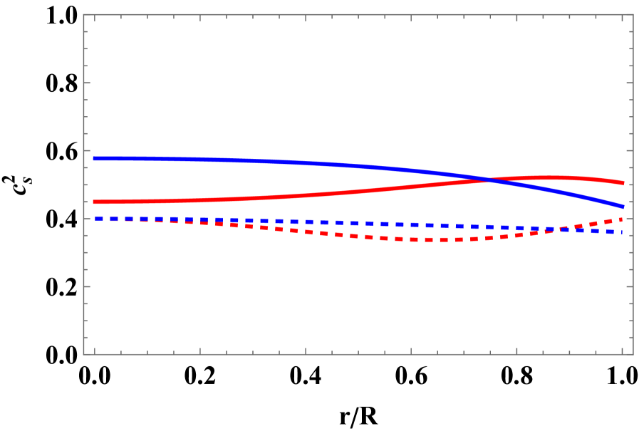
Figure 1: The radial (continuous lines) and angular (dashed lines) sound speeds as functions of the star radius. The theory considered has $\nu=2$. The red lines correspond to $\alpha=0.1$ and the blue ones to $\alpha=0.01$. For the rest of the parameters we have $r_{1}=r_{2}=10$ km and $Q_{0}=1/100$ km^-2.

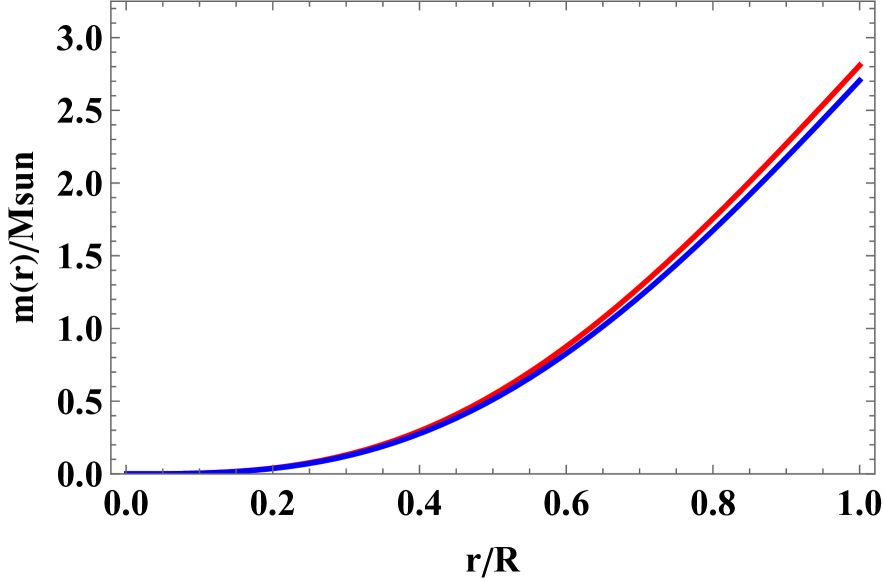
Figure 2: The mass function in the interior of the star. The power index characterizing the theory is $\nu=2$. The red lines correspond to $\alpha=0.1$ and the blue ones to $\alpha=0.01$. For both curves $r_{1}=r_{2}=10$ km and $Q_{0}=1/100$ km^-2.

V Conclusions

In this study, we investigated the structure of static spherically symmetric stars within the framework of symmetric teleparallel $f\left(Q\right)$-gravity. The limit of General Relativity (GR), with or without the cosmological constant, is recovered in $f\left(Q\right)$-theory when $Q$ is constant. Consequently, if $Q$ is a non-zero constant, the de Sitter–Schwarzschild solution emerges.

We exploited this fact to use the latter as the exterior solution of our problem. For the interior of the star, we encountered first the connection which is compatible with the field equations induced by a space-time given by line element (17). It is important to note that this connection can be used in this context with any $f(Q)$ theory. In our investigation we used a power-law $f(Q)$ function (26) and, under the ansatz (27), we determined the physical properties of the respective fluid. We determined variables of the parameters, which give a reasonable behavior for the energy density and the two pressures. We identified the radius $r=\mathcal{R}$, where we assume that $Q(r)=\text{const}$. for $r\geq\mathcal{R}$. In this setting we calculated the explicit expression for the mass function.

Additionally, we analyzed the radial and angular sound speeds near the singularity. For values $\nu>2$ of the power index characterizing the $f\left(Q\right)$-theory, the variation of the sound speeds is nearly independent of $\nu$. These findings contribute to a deeper understanding of the role of nonmetricity in gravitational models and support the viability of $f(Q)$ gravity in describing compact objects. In a future work we plan to study the definition for the Tolman - Oppenheimer - Volkov formula within the symmetric teleparallel theory of gravity.

- (1) M. Tegmark et al., Astrophys. J. 606, 702 (2004)
- (2) M. Kowalski et al., Astrophys. J. 686, 749 (2008)
- (3) E. Komatsu et al., Astrophys. J. Suppl. Ser. 180, 330 (2009)
- (4) N. Suzuki et. al., Astrophys. J. 746, 85 (2012)
- (5) Planck Collaboration: Y. Akrami et al. A&A 641, A10 (2020)
- (6) E. Abdalla et al. JHEAp 34, 49 (2022)
- (7) Y. Carloni, O. Luongo and M. Muccino, Phys. Rev. D 111, 023512 (2025)
- (8) O. Luongo and M. Muccino, Astron. Astrophys. 641, A174 (2020)
- (9) S. Nojiri, S.D. Odintsov and V.K. Oikonomou, Phys. Rept. 692, 1 (2017)
- (10) K. Bamba, LHEP 2022, 352 (2022)
- (11) S. Shankaranarayanan and J.P. Johnson, Gen. Rel. Grav. 54, 44 (2022)
- (12) J.D. Barrow, Phys. Lett. B 214, 515 (1988)
- (13) M. Madsen and J.D. Barrow, Nucl. Phys. B 323, 242 (1989)
- (14) T. Clifton and J.D. Barrow, Phys. Rev. D 72, 123003 (2003)
- (15) T. Clifton and J.D. Barrow, Class. Quantum Grav. 23, 2351 (2006)
- (16) A.A. Starobinsky, Phys. Lett. B 91, 99 (1980)
- (17) T.P. Sotiriou and V. Faraoni, Rev. Mod. Phys. 82, 451 (2010)
- (18) G. Papagiannopoulos, S. Basilakos, J.D. Barrow and A. Paliathanasis, Phys. Rev. D 97, 024026 (2018)
- (19) M. Hohmann, Phys. Rev. D 104, 124077 (2021)
- (20) J. B. Jiménez, L. Heisenberg and T. S. Koivisto, Phys. Rev. D 98, 044048 (2018)
- (21) J. B. Jiménez, L. Heisenberg, T. S. Koivisto and S. Pekar, Phys. Rev. D 101, 103507 (2020)
- (22) S. Bahamonde, J. G. Valcarcel, L. Järv and J. Lember, JCAP 08, 082 (2022)
- (23) L. Järv, M. Rünkla, M. Saal and O. Vilson, Phys. Rev. D 97, 124025 (2018)
- (24) A. Paliathanasis, EPJC 84, 125 (2024)
- (25) A. De, T.-H. Loo and E.N. Saridakis, JCAP 03, 050 (2024)
- (26) A. Paliathanasis, Phys. Dark Universe 43, 101388 (2024)
- (27) S. Nojiri and S.D. Odintsov, F(Q) gravity with Gauss-Bonnet corrections: from early-time inflation to late-time acceleration, (2024) [arXiv:2406.12558]
- (28) L. Heisenberg, Phys. Reports 1066, 1 (2024)
- (29) J. Shi, Eur. Phys. J. C 83, 951 (2023)
- (30) F. K. Anagnostopoulos, S. Basilakos and E. N. Saridakis, Phys. Lett. B 822, 136634 (2021)
- (31) W. Khyllep, A. Paliathanasis and J. Dutta, Phys. Rev. D 103, 103521 (2021)
- (32) A. Lymperis, JCAP 11, 018 (2022)
- (33) J. Ferreira, T. Barreiro, J.P. Mimoso and N.J. Nunes, Phys. Rev. D 108, 063521 (2023)
- (34) M. Koussour, N. Myrzakulov, A.H.A. Alfedeel and E.I. Hassan, Commun. Theor. Phys. 75, 125403 (2023)
- (35) A. Paliathanasis, Phys. Dark Univ. 41, 101255 (2023)
- (36) A. Paliathanasis, Phys. Dark. Univ. 46, 101585 (2024)
- (37) N. Dimakis, A. Paliathanasis, M. Roumeliotis and T. Christodoulakis, Phys. Rev. D 106, 043509 (2022)
- (38) S. Pradhan, R. Solanki and P.K. Sahoo, JHEAp 43, 258 (2024)
- (39) H. Shabani, A. De, T.-H. Loo and E.N. Saridakis, EPJC 84, 285 (2024)
- (40) G. Subramaniam, A. De, T.-H. Loo and Y.K. Goh, Phys. Dark Univ. 41, 101243 (2023)
- (41) S. Nojiri and S.D. Odintsov, Phys. Dark Univ. 45, 101538 (2024)
- (42) Y. Carloni and O. Luongo, arXiv:2410.10935 (2024)
- (43) D.A. Gomes, J.B. Jimenez, A.J. Cano and T.S. Koivisto, Phys. Rev. Lett. 132, 141401 (2024)
- (44) L. Heisenberg and M. Hohmann, JCAP 03, 063 (2024)
- (45) F. D’ Ambrosio, S. D. B. Fell, L. Heisenberg and S. Kuhn, Phys. Rev. D 105, 024042 (2022)
- (46) N. Dimakis, P.A. Terzis, A. Paliathanasis and T. Christodoulakis, JHEAp 45, 273 (2025)
- (47) D. J. Gogoi, A. Övgün and M. Koussour, Eur. Phys. J. C 83, 700 (2023)
- (48) Z.-X. Zhang, C. Lan and Y.-G. Miao, Comparison of Quasinormal Modes of Black Holes in and Gravity, (2025) [arXiv:2501.12800 [gr-qc]]
- (49) S. Bahamonte, J.G. Valcarel, L. Jarv and J. Lember, JCAP 08, 082 (2022)
- (50) S. Bahamonde and L. Järv, Eur. Phys. J. C 82, 963 (2022)
- (51) W. Wang, K. Hu and T. Katsuragawa, Phys. Rev. D 111, 064038 (2025)
- (52) S. Mandal, S. Pradhan, P.K. Sahoo and Tiberiu Harko, Eur. Phys. J. C 83, 1141 (2023)
- (53) D. Mhamdi, F. Bargach, S. Dahmani, A. Bouali and T. Ouali, Phys. Lett. B 859, 139113 (2024)
- (54) J. B. Jimenez, L. Heisenberg and T. S. Koivisto, Universe 5, 173 (2019)
- (55) J. B. Jiménez, L. Heisenberg and T.S. Koivisto, JCAP 08, 039 (2018)
- (56) M. Hohmann, Universe 7, 114 (2021)
- (57) D. Zhao, Eur. Phys. J. C 82, 303 (2022)
- (58) L. P. Eisenhart, “Non-Riemannian Geometry,” American Mathematical Society, Colloquium Publications Vol. VIII, New York, (1927)
- (59) M. Hohmann, Symmetry 12, 53 (2020)
- (60) K.D. Krori and J. Barua, J. Phys. A.: Math. Gen. 8, 508 (1975)