Study of gravitational waves from phase transitions in three-component dark matter

Abstract

This paper presents a dark matter model comprising three types of particles with distinct spins, along with a scalar field $\phi$ that mediates interactions between Standard Model particles and dark matter. It discusses the electroweak phase transition following the Big Bang, during which all particles are initially massless due to the inactive Higgs mechanism. As temperature decreases, the effective potential reaches zero at two points, leading to two minima at the critical temperature ($T_{c}$), and eventually to a true vacuum state. The formation of new vacuum bubbles, where electroweak symmetry is broken and particles acquire mass, generates gravitational waves as these bubbles interact with the fabric of space-time. The paper derives the gravitational wave frequency and detection range based on the model’s parameters, aligning with observational data from the Planck satellite and detection thresholds from PandaX-4T and XENONnT. It concludes by comparing the predicted background gravitational wave density with the sensitivities of LISA and BBO detectors.

1 Introduction

After the Big Bang, all particles, including dark matter particles undergoes a electroweak phase transition at a certain temperature. We present a dark matter model composed of three types of particles, each with distinct spins, along with a scalar field $\phi$ that serves as an intermediary between Standard Model particles and dark matter, capable of assuming the vacuum expectation value. Prior to electroweak phase transition, three-component dark matter particles and all SM particles are massless, because the Higgs mechanism has not yet activated. Before the electroweak phase transition, the minimum of effective potential at a certain value of the scalar field $\phi$ is equal to zero, which indicates the initial vacuum before the phase transition. As the temperature decreases, the effective potential becomes zero at two distinct points of the scalar field $\phi$, resulting in two minima corresponding to the critical temperature ($T_{c}$). As the temperature continues to drop, the potential reaches a distinct negative value, leading to a single minimum known as the ”true vacuum”. Cosmic phase transitions happen when the temperature decreases below a critical level, resulting in the Universe transitioning from a symmetric phase to one characterized by broken symmetry. This temperature, at which the cores of true vacuum bubbles begin to form in space, is known as the nucleation temperature ($T_{n}$). In fact, with the breaking of symmetry, the scalar field ($\phi$) acquires a nonzero vacuum expectation value (VEV), and all particles gain mass through the Higgs mechanism. New vacuum bubbles form spherically and move through space, replacing the vacuum before the phase transition. Inside the bubbles, electroweak symmetry is broken, and the Higgs mechanism is activated. In fact, inside the bubbles, dark matter and Standard Model particles have mass, whereas outside these bubbles, they are massless [1, 2, 3, 4, 5, 6, 7, 8, 9, 10].

The motion of spherically shaped new vacuum bubbles (true vacuum) within the hot plasma resulting from the Big Bang leads to expansion and oscillation in the space-time fabric due to the distribution of mass in space. When the walls of the bubbles collide with each other, they shake the surrounding space-time, which generates gravitational waves that propagate through space. These gravitational waves were produced in the early universe, and their strength has diminished significantly over time and the expansion of the universe, ultimately transforming into cosmic background gravitational waves. In this paper, we derive the GW frequency and range for the detection of these background gravitational waves, considering the assumption of the existence of multi-component dark matter [11, 12, 13, 14, 15, 16, 17, 18, 19, 20].

In this article, we first present the Lagrangian and its dependent constraints for our dark matter model based on WIMPs. In our model, a pair is considered for the Higgs particle, and its mass ($M_{H_{2}}$) is determined by the Gildener–Weinberg mechanism. Next, we select points from our model’s parameter space where their relic density aligns with the Planck satellite report and their rescaled DM-nucleon cross sections exceed the PandaX-4T and XENONnT detection threshold. We then calculate the effective potential for these points and, using the Euclidean action, determine the necessary parameters for background gravitational waves, which we substitute into the relevant equations. Finally, We determine the detection range for the background gravitational wave density using a three-component dark matter model and compare it to the sensitivities of the LISA and BBO gravitational wave detectors [21, 22, 23, 24, 25, 26, 27, 28].

The paper is organized as follows: Section 2 introduces the Lagrangian of our model, while Section 3 examines the electroweak phase transition via the one-loop effective potential. In Section 4, we present our results, considering the gravitational wave spectrum using two selected points outlined in Table 2. We conclude in Section 5.

2 The model

2.1 Lagrangian of model

In this section, we use a model for dark matter that we previously introduced in our earlier article [3]. We proposed a model featuring a scalar field $S$, two spinor fields $\psi^{1,2}$ (including right-handed $\psi^{1,2}_{R}$ and left-handed $\psi^{1,2}_{L}$), and a vector field $V_{\mu}$ as dark matter (DM), along with a complex scalar field $\phi$ acting as an intermediate particle. All these fields are singlets under the Standard Model gauge group. We introduce a discrete symmetry under which the new fields transform as follows:

$$\phi\rightarrow\phi^{*},\quad S\rightarrow-S,\,\quad V_{\mu}\rightarrow-V_{\mu},\,\quad\psi_{L}^{1}\rightarrow-\psi_{L}^{2}\quad\text{and}\,\quad\psi_{R}^{1}\rightarrow-\psi_{R}^{2}.$$ (2.1)

All SM particles are even and singlets under the dark gauge symmetry. The local gauge transformation for the new fields is as follows:

$$S\rightarrow e^{iQ_{S}\alpha(x)}S,$$

$$\psi_{L}^{a}\rightarrow e^{iQ_{L}^{a}\alpha(x)}\psi_{L}^{a},$$

$$\psi_{R}^{a}\rightarrow e^{iQ_{R}^{a}\alpha(x)}\psi_{R}^{a},$$

$$\phi\rightarrow e^{iQ_{\phi}\alpha(x)}\phi,$$

$$V_{\mu}\rightarrow V_{\mu}-\frac{1}{g_{v}}\partial_{\mu}{\alpha(x)}.$$ (2.2)

In our model, the scalar field $\phi$ and the spinor fields $\psi^{1,2}_{R}$ and $\psi^{1,2}_{L}$ carry charge under a dark $U_{D}(1)$ gauge symmetry, with the vector field $V_{\mu}$ acting as the gauge field (see Table 1).

Table 1: The charges associated with the particles in the dark sector with respect to the newly introduced $U_{D}(1)$ symmetry.

field	$\phi$	$S$	$V_{\mu}$	$\psi_{L}^{1}$	$\psi_{R}^{1}$	$\psi_{L}^{2}$	$\psi_{R}^{2}$
dark charge ($Q$)	$1$	0	0	$\frac{1}{2}$	$-\frac{1}{2}$	$-\frac{1}{2}$	$\frac{1}{2}$

We present the Lagrangian, invariant under the local gauge transformation (2.1) and incorporating renormalizable interactions, as follows:

$${\cal L}={\cal L}_{SM}+\frac{1}{2}(\partial_{\mu}S)(\partial^{\mu}S)+(D_{\mu}\phi)^{*}(D^{\mu}\phi)-\frac{1}{4}V_{\mu\nu}V^{\mu\nu}-V(H,S,\phi)$$

$$+\sum_{a=1}^{2}\left(i\bar{\psi}_{L}^{a}\gamma^{\mu}D_{\mu}\psi_{L}^{a}+i\bar{\psi}_{R}^{a}\gamma^{\mu}D_{\mu}\psi_{R}^{a}\right)-g_{\phi,1}\phi\bar{\psi}_{L}^{1}\psi_{R}^{1}-g_{\phi,2}\phi^{*}\bar{\psi}_{L}^{2}\psi_{R}^{2}+{\text{H.C.}},$$ (2.3)

where ${\cal L}_{SM}$ is the SM Lagrangian without the Higgs potential term. The covariant derivative and field strength tensor are $D_{\mu}=(\partial_{\mu}+iQg_{v}V_{\mu})$ and $V_{\mu\nu}=\partial_{\mu}V_{\nu}-\partial_{\nu}V_{\mu}$, respectively. From (2.1), we have $g_{\phi,1}=g_{\phi,2}=g_{\phi}$, leading to $M_{\psi_{1}}=M_{\psi_{2}}=M_{\psi}$. We introduce gauge invariant potential $V(H,\phi,S)$ as follows:

$$V(H,\phi,S)= \,\lambda_{H}(H^{\dagger}H)^{2}+\lambda_{\phi}(\phi^{*}\phi)^{2}+\lambda_{H\phi}(H^{\dagger}H)(\phi^{*}\phi)$$

$$+\frac{1}{2}\lambda_{HS}(H^{\dagger}H)S^{2}+\frac{1}{2}\lambda_{\phi S}(\phi^{*}\phi)S^{2}+\frac{1}{4}\lambda_{S}S^{4}.$$ (2.4)

Since all the particles introduced as dark matter are odd, no interaction occurs between them, leading to an accidental symmetry that allows dark matter to persist. The scalar field $\phi$ can acquire VEVs that break the $U_{D}(1)$ symmetry, while the Higgs field $H$ can obtain VEVs that break electroweak symmetry. We can rewrite the scalar and Higgs fields in unitary gauge as follows:

$$H=\frac{1}{\sqrt{2}}\begin{pmatrix}0\\ h_{1}\end{pmatrix}\,\,\,and\,\,\,\phi=\frac{1}{\sqrt{2}}h_{2}.$$ (2.5)

Here, $h_{1}$ and $h_{2}$ are real scalar fields that can acquire vacuum expectation values. By substituting Eqs. (2.5) into Eq. (2.1), the tree-level potential can be rewritten as follows:

$$V^{tree}=\frac{1}{4}\lambda_{H}h_{1}^{4}+\frac{1}{4}\lambda_{\phi}h_{2}^{4}+\frac{1}{4}\lambda_{\phi H}h_{1}^{2}h_{2}^{2}+\frac{1}{4}\lambda_{HS}h_{1}^{2}s^{2}+\frac{1}{4}\lambda_{\phi S}h_{2}^{2}s^{2}+\frac{1}{4}\lambda_{s}s^{4}.$$ (2.6)

The local minimum of the tree-level potential (2.6) at $\langle h_{1}\rangle=\nu_{1}$ and $\langle h_{2}\rangle=\nu_{2}$ defines the VEVs of the fields, leading to the following condition:

$$\lambda_{\phi H}<0\;\;,\;\;\lambda_{H}>0\;\;,\;\;\lambda_{\phi}>0$$

$$\frac{\nu_{1}^{2}}{\nu_{2}^{2}}=-\frac{\lambda_{\phi H}}{2\lambda_{H}}\;\;,\;\;\frac{\nu_{2}^{2}}{\nu_{1}^{2}}=-\frac{\lambda_{\phi H}}{2\lambda_{\phi}},$$

$$\;\;\;\;\;\;\;\;\;\;\;\;\lambda_{\phi H}^{2}=4\lambda_{H}\lambda_{\phi}.$$ (2.7)

In the flat direction of field space, the tree-level potential reaches its minimum, along which $V_{\text{tree}}(\nu_{1},\nu_{2},0)=0$. Now, we substitute $h_{1}\to\nu_{1}+h_{1}$ and $h_{2}\to\nu_{2}+h_{2}$, mixing $h_{1}$ and $h_{2}$. The mass eigenstates, $H_{1}$ and $H_{2}$, can be obtained from the following rotation:

$$\begin{bmatrix}H_{1}\\ H_{2}\end{bmatrix}=\begin{bmatrix}\cos\alpha&-\sin\alpha\\ \sin\alpha&\;\;\;\cos\alpha\end{bmatrix}\begin{bmatrix}h_{1}\\ h_{2}\end{bmatrix}.$$ (2.8)

The rotation of the fields in (2.8), the flat direction position and ($\alpha$) angle are shown in figure 1. The mass of $H_{1}$ and $H_{2}$ are determined by substituting (2.8) into (2.6) and calculating $M_{H_{i}}^{2}=\frac{\partial^{2}V^{\text{tree}}}{\partial H_{i}^{2}}$, as follows:

$$M_{H_{1}}^{2}=-H_{2}^{2}\lambda_{\phi H},$$ (2.9)

$$M_{H_{2}}^{2}=-H_{1}^{2}\lambda_{\phi H}.$$ (2.10)

Equation (2.9) and (2.10) are derived from the flat direction situation. Equation (2.10) shows that the mass of $H_{2}$ is influenced by the $H_{1}$ field, so in the flat direction where $H_{1}=0$, as illustrated in figure 1, the mass of $H_{2}$ is zero. The $H_{1}$ field is perpendicular to the flat direction and is identified as the SM-like Higgs observed at the LHC, leading us to consider $M_{H_{1}}=125\;GeV$ [29]. Figure 1 shows that at every point along the flat direction line, the value of $H_{2}$ equals the hypotenuse.

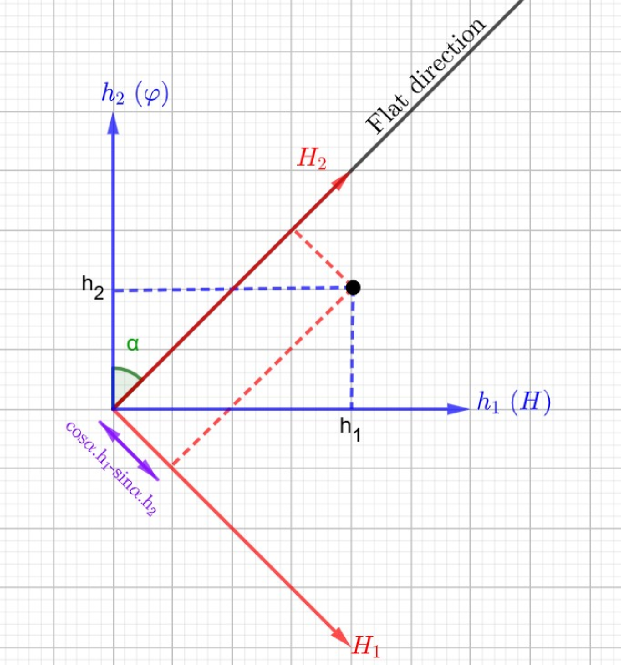
Figure 1: The relative positions of the Higgs and scalar fields as indicated in (2.8).

Consequently, the average $<H_{2}>$ in the flat direction is calculated as follows:

$$<H_{2}>=\sqrt{\nu_{1}^{2}+\nu_{2}^{2}}=\nu.$$ (2.11)

On the other hand, from the Standard Model, we know that $\nu_{1}=246\;GeV$. As mentioned before, the field $H_{2}$ is aligned along the flat direction; thus, its tree-level mass is zero. However, the inclusion of one-loop corrections via Gildener–Weinberg mechanism leads to a non-zero value along the flat direction, yielding a minimum of the potential, which provides the following mass to $H_{2}$:

$$M_{H_{2}}^{2}=\frac{1}{8\pi^{2}\nu^{2}}\left(M_{H_{1}}^{4}+6M_{W}^{4}+3M_{Z}^{4}+3M_{V}^{4}+M_{S}^{4}-8M_{\psi}^{4}-12M_{t}^{4}\right),$$ (2.12)

where $M_{W,Z,V,S,\psi,t}$ being the masses for W and Z gauge bosons, vector DM, scalar DM, spinor DM and top quark, respectively after symmetry breaking. The model’s dependent constraints are obtained as follows:

$$\sin\alpha=\frac{\nu_{1}}{\sqrt{\nu_{1}^{2}+\nu_{2}^{2}}},\;\;g_{V}=\frac{M_{V}}{\nu_{2}},\;\;g_{\phi}=\frac{\sqrt{2}M_{\psi}}{\nu_{2}},$$

$$\lambda_{H}=\frac{M_{H_{1}}^{2}cos^{2}\alpha}{2\nu_{1}^{2}},\;\;\lambda_{\phi}=\frac{M_{H_{1}}^{2}sin^{2}\alpha}{2\nu_{2}^{2}},$$

$$\lambda_{\phi H}=-\frac{M_{H_{1}}^{2}\sin\alpha\cos\alpha}{\nu_{1}\nu_{2}},\;\;\lambda_{HS}=\frac{2M_{S}^{2}-\lambda_{\phi S}\nu_{2}^{2}}{\nu_{1}^{2}}.$$ (2.13)

There are six free parameters which we choose them as $M_{S}$, $M_{V}$, $M_{\psi}$, $\lambda_{\phi s}$, $\nu_{2}$ and $\lambda_{s}$. Conversely, $\lambda_{s}$ is irrelevant to the DM phenomenology and phase transition studied in this paper, leaving us with only four free parameters.

2.2 Appropriate points

In this section, we use the micrOMEGAs to select parameter points from our model that achieve a relic density between 0.10 and 0.14, while also ensuring that their DM-nucleon cross section significantly exceeds the detection threshold of the PandaX-4T and XENONnT detectors [30, 21]. For $M_{DM}>40\;GeV$, the direct detection constraint is expressed as follows:

$$\frac{\sigma}{\text{M}_{\text{DM}}}\equiv\xi_{S}\frac{\sigma_{s}}{M_{S}}+\xi_{\psi}\frac{\sigma_{\psi}}{M_{\psi}}+\xi_{V}\frac{\sigma_{v}}{M_{V}}\lesssim\frac{\sigma}{M}\bigg{\rvert}_{\text{PandaX-4T}}\simeq 0.0005\,\frac{\text{zb}}{\text{GeV}},$$ (2.14)

Where $\xi_{i}$ is the dark matter fractions used to quantify the relative importance of each type of dark matter, as follows:

$$\xi_{S}=\frac{\Omega_{S}}{\Omega_{DM}},\;\;\;\xi_{\psi}=\frac{\Omega_{\psi}}{\Omega_{DM}},\;\;\;\xi_{V}=\frac{\Omega_{V}}{\Omega_{DM}},$$ (2.15)

where $\xi_{S}+\xi_{\psi}+\xi_{V}=1$. Using dark matter relic density measurements from the Planck collaboration and considering (2.14), we identify two suitable points presented in Table 2.

Table 2: Characteristics of the selected points with $\lambda_{\phi s}=8$, according to inequality (2.14).

Point	$M_{V}$(GeV)	$M_{S}$(GeV)	$M_{\psi}$(GeV)	${\nu}_{2}$(GeV)	$M_{H_{2}}$(GeV)	${\Omega}h^{2}$
A	54.5	1125	611	567	125.79	0.12
B	330	665	175	340	124	0.14

Considering the condition $M_{V}<2M_{\psi}$, all scalar, spinor, and vector components are viable DM candidates. Thus, Table 2 shows that for each point, the mass of the vector particle is less than twice that of the spinor particle.

The rescaled DM-nucleon cross sections of selected points, relative to the threshold of the PandaX-4T and XENONnT detectors, are shown in Figure 2.

   

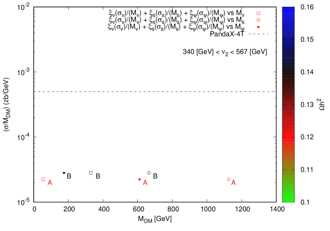
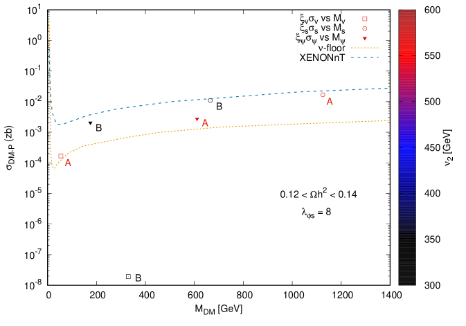
Figure 2: These figures illustrate the points from table 2 in relation to rescaled DM-Proton cross section versus DM masses, with $\nu_{2}$ and ${\Omega}h^{2}$ represented by color bar.

As shown in figure 2, both points selected fall below the PandaX-4T and XENONnT line threshold. Thus, we can use these points to calculate the gravitational waves from the electroweak phase transition.

In the following sections, we will calculate gravitational waves from phase transitions using the points in table 2.

3 Electroweak phase transition

3.1 One-loop effective potential

As the gravitational waves from the electroweak phase transition obtain from the potential, in this section we acquire the effective potential as a function of temperature (T) and the scalar field ($\phi$). The effective potential is the combination of the zero-temperature and non-zero temperature potentials, including the tree-level and daisy potentials. In the flat direction, substituting $H_{1}=0$ and $H_{2}=\nu$ into equation (2.6) results $V^{tree}=0$, as illustrated in equation (2.11). The effective potential is defined as follows:

$$V_{\text{eff}}(\phi,T)=\underbrace{V^{\text{tree}}}_{0}+V_{(T=0)}^{(1-\text{Loop})}+V_{(T\neq 0)}^{(1-\text{Loop})}+V_{\text{daisy}}$$ (3.1)

The effective potential was initially studied at the 1-loop level by Coleman and Weinberg. The Coleman–Weinberg potential is a sum of 1PI 1-loop diagrams featuring arbitrary numbers of external fields and particles in the loops [31]. Then Gildener and Weinberg presented their formulation for a scale-invariant theory involving multiple scalar fields [32]. The Gildener and Weinberg potential is as follows:

$$V_{\text{GW}}^{(1-\text{Loop})}=a\phi^{4}+b\phi^{4}\ln\left(\frac{\phi^{2}}{\Lambda^{2}}\right),$$ (3.2)

where

$$a =\frac{1}{64\pi^{2}\nu^{4}}\sum_{k=1}^{n}g_{k}M_{k}^{4}\left(\ln\frac{M_{k}^{2}}{\nu^{2}}-C_{k}\right),$$

$$b =\frac{1}{64\pi^{2}\nu^{4}}\sum_{k=1}^{n}g_{k}M_{k}^{4}.$$ (3.3)

In equation (3.2) $\Lambda$ is the renormalization group (RG) scale. In equation (3.1) the $C_{k}$=3/2 (5/6), $M_{k}$ and $g_{k}$ are scalars/spinors (vectors), the measured mass of particles, and the number of degrees of freedom of particle k, respectively. By finding the minimum of potential (3.2) at $\phi\neq 0$, the VEV value becomes non-zero:

$$\frac{dV^{1\text{-loop}}}{d\varphi}\bigg{|}_{\langle\varphi\rangle\neq 0} =0,$$

$$\frac{d^{2}V^{1\text{-loop}}}{d\varphi^{2}}\bigg{|}_{\langle\varphi\rangle\neq 0} >0,$$ (3.4)

which leads to

$$\langle\varphi\rangle=\nu=\Lambda e^{-\left(\frac{a}{2b}+\frac{1}{4}\right)}\quad\text{and}\quad b>0.$$ (3.5)

By substituting (3.5) and (3.1) into equation (3.2), we obtain the effective potential at the $T=0$ as follows:

$$V_{(T=0)}^{(1\text{-Loop})}(\varphi)=\frac{M_{H_{2}}^{2}}{8\nu^{2}}\varphi^{4}\left(\ln\left(\frac{\varphi^{2}}{\nu^{2}}\right)-\frac{1}{2}\right).$$ (3.6)

We now examine the finite-temperature 1-loop effective potential, allowing us to compute the scalar field vacuum expectation values in a thermal bath at temperature T [33]. The 1-loop finite-temperature corrections are given by

$$V_{(T\neq 0)}^{(1\text{-Loop})}(\varphi,T)=\frac{T^{4}}{2\pi^{2}}\sum_{i=1}^{n}g_{k}J_{(B,F)_{i}}(x),\quad x=\frac{M_{i}\varphi}{\nu T},$$ (3.7)

where $J_{(B_{i})}(x)$ and $J_{(F_{i})}(x)$ are thermal functions defined as follows:

$$J_{(B_{i})}(x) =-\sum_{k=1}^{3}\frac{1}{k^{2}}x^{2}k_{2}(kx),$$

$$J_{(F_{i})}(x) =-\sum_{k=1}^{2}\frac{(-1)^{k}}{k^{2}}x^{2}k_{2}(kx).$$ (3.8)

Since we have only calculated the potential for one-loop Feynman diagrams so far, it is necessary to compute the potential for higher-order corrections of Feynman diagrams as well. For this purpose, we will use the daisy potential. We have obtained two types of potentials from the total effective potential, with the daisy potential being the last component. The daisy potential includes thermal contributions from virtual particles at finite temperatures, modifying the effective potential by incorporating thermal excitations. Daisy diagrams serve as higher loop corrections that capture the effects of thermal fluctuations and interactions among virtual particles, making the effective potential temperature-dependent, especially during phase transitions. This non-perturbative effect reflects significant feedback from these loop corrections, leading to important physical insights that traditional perturbative approaches might miss. The daisy potential is defined as follows [34]:

$$V_{\text{daisy}}(\varphi,T)=\sum_{k=1}^{n}\frac{g_{k}T^{4}}{12\pi}\left(x^{3}-\left(x^{2}+\frac{\prod_{k}}{T^{2}}\right)^{\frac{3}{2}}\right),\quad x=\frac{M_{i}\varphi}{\nu T},$$ (3.9)

where the sum includes only scalar bosons and the longitudinal degrees of freedom of the gauge bosons. In equation (3.9), the $\prod_{k}$ are the thermal masses of particle k, defined as follows:

$$\Pi_{s} =\frac{T^{2}}{24}\left(\lambda_{HS}+6\lambda_{S}+\lambda_{\phi S}\right),$$

$$\Pi_{w} =\frac{11}{6}(g_{SM}^{2}T^{2}),\quad g_{SM}=\frac{2M_{w}}{\nu_{1}},$$

$$\Pi_{V} =\frac{2}{3}(g_{V}^{2}T^{2}),\quad g_{V}=\frac{M_{V}}{\nu_{2}},$$

$$\Pi_{Z} =\frac{11}{6}(g_{SM}^{2}T^{2}),$$

$$\Pi_{H_{1}} =\frac{T^{2}}{24}\left(\frac{9}{2}g_{SM}^{2}+\frac{3}{2}g_{SM}^{\prime 2}+6\lambda_{t}^{2}+\lambda_{H}\phi+6\lambda_{H}+\lambda_{HS}\right),\quad g_{SM}^{\prime}=\frac{2\sqrt{M_{Z}^{2}-M_{w}^{2}}}{\nu_{1}},$$

$$\lambda_{t} =\frac{\sqrt{2}M_{t}}{\nu_{1}},$$ (3.10)

where $\lambda_{t}$ denotes the top quark Yukawa coupling, and $g_{v}$, $g_{SM}$, and $g_{SM}^{\prime}$ are dark $U(1)_{D}$, $SU(2)_{L}$, and $U(1)_{Y}$ gauge couplings, respectively. The parameters values from (2.13) are utilized to calculate the thermal masses in (3.1). Finally, we can express the total effective potential (3.1) in terms of temperature (T) and the scalar field ($\phi$). We can now substitute the effective potential into the Euclidean action. The function $S_{3}(T)$ represents the three-dimensional Euclidean action for a spherically symmetric bubble, defined as follows:

$$S_{3}(T)=4\pi\int_{0}^{\infty}dr\,r^{2}\left(\frac{1}{2}\left(\frac{d\varphi}{dr}\right)^{2}+V_{\text{eff}}(\varphi,T)\right),$$ (3.11)

where $\phi$ fulfills the differential equation that minimizes $S_{3}(T)$:

$$\frac{d^{2}\varphi}{dr^{2}}+\frac{2d\varphi}{rdr}=\frac{\partial V_{\text{eff}}(\varphi,T)}{\partial\varphi},$$ (3.12)

with the following boundary conditions:

$$\frac{d\varphi}{dr}\bigg{|}_{r=0}=0,\quad\text{and}\quad\varphi(r\to\infty)=0.$$ (3.13)

The nucleation temperature ($T_{n}$) occurs where the corresponding euclidean action is $S_{E}=\frac{S_{3}(T_{N})}{T_{N}}\simeq 140$ [24]. To solve equation (3.12) and find the Euclidean action (3.11), we used the AnyBubble package [23]. This package allows us to calculate the Euclidean action for each selected point using the two minima in the effective potential diagram as function of the scalar field ($\phi$), and plot the ratio of the Euclidean action to temperature (T). In figure 3, we present $\frac{S_{3}(T)}{T}$ for selected points in table 2.

   

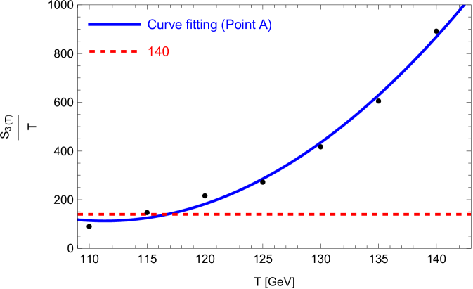
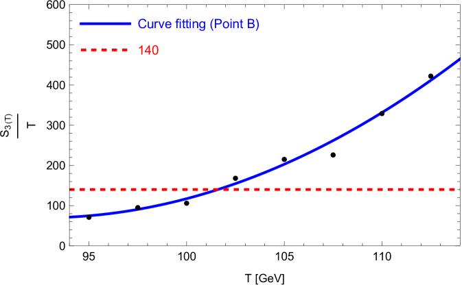
Figure 3: The blue line shows $S_{3}(T)/T$ as a function of T, while the dashed red line indicates $S_{3}(T)/T$ = 140, where nucleation occurs. The black dots are derived using the AnyBubble package.

In figure 3, the nucleation temperature ($T_{n}$) is determined by finding the intersection point of the curve fitting and the red line.

To determine the critical temperature $T_{c}$ for the points in table 2, we must plot the effective potential (3.1) against the scalar field ($\phi$) to identify the temperature at which the effective potential exhibits two aligned minima (see figure 4).

   

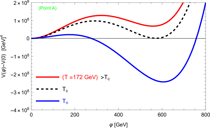
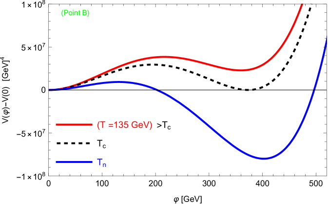
Figure 4: Effective potential diagrams of points in table 3 as a function of $\phi$ scalar field at nucleation, critical, and supercritical temperatures.

Figure 4 shows the effective potential for each point in Table 2 at the three temperatures: nucleation ($T_{n}$), critical ($T_{c}$), and supercritical ($T>T_{c}$). To ensure $V_{\text{eff}}(0,T)=0$ at all temperatures, we subtract a constant term from the potential: $V_{\text{eff}}(\phi,T)\rightarrow V_{\text{eff}}(\phi,T)-V_{\text{eff}}(0,T)$. As shown in Figure 4, at the nucleation temperature ($T_{n}$), the zero minimum is known as a false vacuum and the negative minimum is known as a true vacuum. There is a bulge between the two minima, which prevents the electroweak phase transition from occurring smoothly between the minima, and instead occurs suddenly and explosively, like a dam breaking.

The supercritical temperatures ($T>T_{c}$) shown in figure 4 are determined as arbitrary and indicate the position of the effective potential in relation to the nucleation and critical temperatures. Figure 4 illustrates that as the temperature decreased, the effective potential also diminishes. Table 3 specifies the calculated values for the nucleation and critical temperatures, as follows:

Table 3: The nucleation and critical temperatures according to points of table 2.

Point	$T_{n}$(GeV)	$T_{C}$(GeV)	${\phi}_{V_{min}}$(GeV)
A	116	162.5	606.022
B	101	128.2	402.363

In Table 3, the ${\phi}_{V_{min}}$ denotes the point of ${\phi}$ scalar field at which the effective potential value in $T_{n}$ is minimized, as illustrated in Figure 4. In this context, the ${\phi}_{V_{min}}$ represents the true vacuum.

In the next section, we will use the values from Table 3 to calculate the background gravitational waves.

3.2 Gravitational waves

The background gravitational waves from strong first-order electroweak phase transitions has three contributions:

1. The collision of spherical bubble walls in the plasma after the Big Bang.

2. Sound waves that release kinetic energy in the plasma due to bubble collisions.

3. Turbulence of massive plasma in the fabric of space-time.

Before calculating gravitational waves, we need to introduce $\alpha$ (the strength parameter) and $\beta$, the inverse duration of the phase transition, as follows:

$$\alpha=\frac{\Delta\left(V_{\text{eff}}-T\frac{\partial V_{\text{eff}}}{\partial T}\right)_{\big{|}_{T_{n}}}}{\rho_{*}},\;\;\;\rho_{*}=\frac{\pi^{2}g_{*}}{30}T_{n}^{4}$$

$$\frac{\beta}{H_{*}}=T_{n}\left.\frac{d}{dT}\left(\frac{S_{3}(T)}{T}\right)\right|_{T_{n}},$$ (3.14)

where $g_{*}=100$. In equation (3.2), we obtain the parameter $\frac{\beta}{H_{*}}$ from the slope of the graphs in figure 3 at the intersection point of the curve fitting and the red line. Now, we derive the density relations of gravitational waves for all three types of their sources, including collision (coll), sound wave (sw), and turbulence (turb). We begin with the density of background gravitational waves from collision sources [35]:

$$\Omega_{\text{coll}}(f)h^{2}=1.67\times 10^{-5}\left(\frac{\beta}{H_{*}}\right)^{-2}\left(\frac{k\alpha}{1+\alpha}\right)^{2}\left(\frac{g_{*}}{100}\right)^{-\frac{1}{3}}\left(\frac{0.11v_{w}^{3}}{0.42+v_{w}^{2}}\right)S_{\text{coll}},$$ (3.15)

where k is the fraction of latent heat converted into the gradient energy of the Higgs-like field, defined as follows:

$$k=\frac{1}{1+0.715\alpha}\left(0.715\alpha+\frac{4}{27}\sqrt{\frac{3\alpha}{2}}\right).$$ (3.16)

In equation (3.15), $v_{w}$ is the bubble propagation speed, which we take to be equal to one [36]. Additionally, f is the GW frequency of the gravitational wave. $S_{\text{coll}}$ is the spectral shape parameter of the bubble, defined by the following relation:

$$S_{\text{coll}}=\frac{3.8\left(\frac{f}{f_{\text{coll}}}\right)^{2.8}}{2.8\left(\frac{f}{f_{\text{coll}}}\right)^{3.8}+1},$$

$$f_{\text{coll}}=1.65\times 10^{-5}\left(\frac{0.62}{v_{w}^{2}-0.1v_{w}+1.8}\right)\left(\frac{\beta}{H_{*}}\right)\left(\frac{T_{n}}{100}\right)\left(\frac{g_{*}}{100}\right)^{\frac{1}{6}}.$$ (3.17)

The density of background GW from sound wave sources is defined as [37]:

$$\Omega_{\text{sw}}(f)h^{2}=2.65\times 10^{-6}\left(\frac{\beta}{H_{*}}\right)^{-1}\left(\frac{k_{v}\alpha}{1+\alpha}\right)^{2}\left(\frac{g_{*}}{100}\right)^{-\frac{1}{3}}v_{w}S_{\text{sw}},$$ (3.18)

where $k_{v}$ is the bulk motion of the fluid, defined as follows:

$$k_{v}=\frac{\alpha}{0.73+0.083\sqrt{\alpha}+\alpha}.$$ (3.19)

In equation (3.18), $S_{\text{sw}}$ is also the spectral shape parameter of the bubble, defined as follows:

$$S_{\text{sw}} =\left(\frac{f}{f_{\text{sw}}}\right)^{3}\left(\frac{7}{3\left(\frac{f}{f_{\text{sw}}}\right)^{2}+4}\right)^{3.5},$$

$$f_{\text{sw}} =1.9\times 10^{-5}\left(\frac{1}{v_{w}}\right)\left(\frac{\beta}{H_{*}}\right)\left(\frac{T_{n}}{100}\right)\left(\frac{g_{*}}{100}\right)^{\frac{1}{6}}.$$ (3.20)

The density of background GW from turbulence sources is defined as [38]:

$$\Omega_{\text{turb}}(f)h^{2}=3.35\times 10^{-4}\left(\frac{\beta}{H_{*}}\right)^{-1}\left(\frac{k_{\text{turb}}\alpha}{1+\alpha}\right)^{\frac{3}{2}}\left(\frac{g_{*}}{100}\right)^{-\frac{1}{3}}v_{w}S_{\text{turb}},$$ (3.21)

where $k_{\text{turb}}$ is the magneto-hydrodynamic (MHD) turbulence, defined as follows:

$$k_{\text{turb}}=0.05k_{v}$$ (3.22)

In equation (3.21), $S_{\text{turb}}$ is defined as follows:

$$S_{\text{turb}} =\frac{\left(\frac{f}{f_{\text{turb}}}\right)^{3}}{\left(1+\frac{8\pi f}{h_{*}}\right)\left(1+\frac{f}{f_{\text{turb}}}\right)^{\frac{11}{3}}},\;\;\;h_{*}=1.65\times 10^{-5}\left(\frac{T_{n}}{100}\right)\left(\frac{g_{*}}{100}\right)^{\frac{1}{6}},$$

$$f_{\text{turb}} =2.7\times 10^{-5}\left(\frac{1}{v_{w}}\right)\left(\frac{\beta}{H_{*}}\right)\left(\frac{T_{n}}{100}\right)\left(\frac{g_{*}}{100}\right)^{\frac{1}{6}}.$$ (3.23)

In the next section, we plot all types of background gravitational wave densities obtained in terms of GW frequency.

4 Results

In this section, we calculate $\alpha$ as the strength parameter and $\beta$ as the inverse duration of the phase transition, for selected points, as shown in Table 4.

Table 4: Phase transition parameters based on (3.2) for the points in Table 2.

Point	$T_{n}$(GeV)	$\alpha$	$\frac{\beta}{H_{*}}$
A	116	0.1119	1004
B	101	0.0970	1469

Now by using the previous section’s relations and the results of table 4, we can determine the total background gravitational wave density from the electroweak phase transition as follows:

$$\Omega_{\text{total}}(f)h^{2}\simeq\Omega_{\text{coll}}(f)h^{2}+\Omega_{\text{sw}}(f)h^{2}+\Omega_{\text{turb}}(f)h^{2}.$$ (4.1)

Finally, figure 5 presents the total background gravitational wave density (4.1) versus GW frequency, utilizing data from table 4 for selected points. In figure 5, there are two curves for Lisa and BBO, which show the power of space-based laser detectors that have not yet been launched into space. As shown in figure 5, the Lisa detector does not have the capability to detect the background gravitational waves resulting from the electroweak phase transition for parameter space of B point; however, it is possible that other points like A, in our model exist where Lisa could detect the background gravitational waves from their electroweak phase transitions.

   

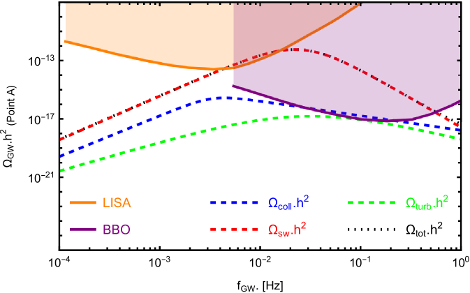
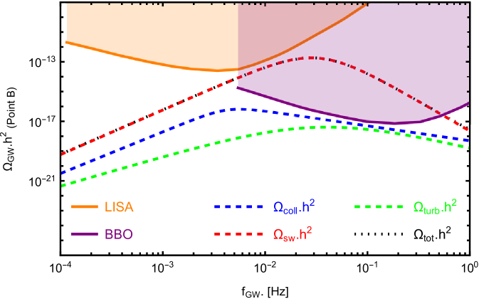
Figure 5: GW spectrum as a function of backgound gravitational frequency for points in Table 4.

In contrast, the BBO detector can detect a portion of these background gravitational waves for both points.

The background gravitational wave density from sound wave sources in both graphs in figure 5 is the main contributor to the total background gravitational wave. The maximum values in both graphs, indicate that the optimal GW frequency range for detecting background gravitational waves is between 0.003 and 0.5 Hz, with the best GW frequency at 0.02 Hz.

5 Conclusion

This paper introduces a model of dark matter in which particles exhibit three spin types: a vector particle, a scalar, and a spinor. In our model, the Higgs particle acts as a portal between Standard Model particles and dark matter. We identified parameter space points that exceed the detection capability of PandaX-4T and XENONnT, while their relic density matches the Planck satellite’s findings. We examined the electroweak phase transition for these points and showed that a potential barrier between the two minima of the effective potential at nucleation temperature can generate gravitational waves. The three parameters, $\alpha$, $\frac{\beta}{H_{*}}$, and nucleation temperature ($T_{n}$), are sufficient for gravitational wave calculations, independent of other model parameters. Our results indicate that the sensitivity of the LISA detector is insufficient for detecting cosmic background gravitational waves throughout the entire parameter space within the three-component dark matter model, whereas the BBO detector has the capability to confirm the existence of these waves.

References

- [1] K. M. Zurek, Phys. Rev. D 79 (2009), 115002 doi:10.1103/PhysRevD.79.115002 [arXiv:0811.4429 [hep-ph]].
- [2] A. Biswas, D. Majumdar, A. Sil and P. Bhattacharjee, JCAP 12 (2013), 049 doi:10.1088/1475-7516/2013/12/049 [arXiv:1301.3668 [hep-ph]].
- [3] M. H. R. Abkenar, A. Mohamadnejad and R. Sepahvand, Phys. Rev. D 111 (2025) no.5, 055018 doi:10.1103/PhysRevD.111.055018 [arXiv:2410.22252 [hep-ph]].
- [4] S. Yaser Ayazi and A. Mohamadnejad, Eur. Phys. J. C 79 (2019) no.2, 140 doi:10.1140/epjc/s10052-019-6651-5 [arXiv:1808.08706 [hep-ph]].
- [5] A. H. Guth and E. J. Weinberg, Phys. Rev. D 23 (1981), 876 doi:10.1103/PhysRevD.23.876
- [6] P. J. Steinhardt, Phys. Rev. D 25 (1982), 2074 doi:10.1103/PhysRevD.25.2074
- [7] E. Witten, Nucl. Phys. B 177 (1981), 477-488 doi:10.1016/0550-3213(81)90182-6
- [8] P. J. Steinhardt, Nucl. Phys. B 179 (1981), 492-508 doi:10.1016/0550-3213(81)90016-X
- [9] E. Witten, Phys. Rev. D 30 (1984), 272-285 doi:10.1103/PhysRevD.30.272
- [10] S. Yaser Ayazi and A. Mohamadnejad, JHEP 03 (2019), 181 doi:10.1007/JHEP03(2019)181 [arXiv:1901.04168 [hep-ph]].
- [11] E. Hall, T. Konstandin, R. McGehee and H. Murayama, Phys. Rev. D 107 (2023) no.5, 055011 doi:10.1103/PhysRevD.107.055011 [arXiv:1911.12342 [hep-ph]].
- [12] E. Hall, R. McGehee, H. Murayama and B. Suter, Phys. Rev. D 106 (2022) no.7, 075008 doi:10.1103/PhysRevD.106.075008 [arXiv:2107.03398 [hep-ph]].
- [13] E. Hall, T. Konstandin, R. McGehee, H. Murayama and G. Servant, JHEP 04 (2020), 042 doi:10.1007/JHEP04(2020)042 [arXiv:1910.08068 [hep-ph]].
- [14] M. Chala, G. Nardini and I. Sobolev, Phys. Rev. D 94 (2016) no.5, 055006 doi:10.1103/PhysRevD.94.055006 [arXiv:1605.08663 [hep-ph]].
- [15] I. Baldes, JCAP 05 (2017), 028 doi:10.1088/1475-7516/2017/05/028 [arXiv:1702.02117 [hep-ph]].
- [16] R. Flauger and S. Weinberg, Phys. Rev. D 97 (2018) no.12, 123506 doi:10.1103/PhysRevD.97.123506 [arXiv:1801.00386 [astro-ph.CO]].
- [17] W. Chao, H. K. Guo and J. Shu, JCAP 09 (2017), 009 doi:10.1088/1475-7516/2017/09/009 [arXiv:1702.02698 [hep-ph]].
- [18] X. F. Han, L. Wang and Y. Zhang, Phys. Rev. D 103 (2021) no.3, 035012 doi:10.1103/PhysRevD.103.035012 [arXiv:2010.03730 [hep-ph]].
- [19] X. Deng, X. Liu, J. Yang, R. Zhou and L. Bian, Phys. Rev. D 103 (2021) no.5, 055013 doi:10.1103/PhysRevD.103.055013 [arXiv:2012.15174 [hep-ph]].
- [20] K. Kannike and M. Raidal, Phys. Rev. D 99 (2019) no.11, 115010 doi:10.1103/PhysRevD.99.115010 [arXiv:1901.03333 [hep-ph]].
- [21] Y. Meng et al. [PandaX-4T], Phys. Rev. Lett. 127 (2021) no.26, 261802 doi:10.1103/PhysRevLett.127.261802 [arXiv:2107.13438 [hep-ex]].
- [22] N. Aghanim et al. [Planck], Astron. Astrophys. 641 (2020), A6 [erratum: Astron. Astrophys. 652 (2021), C4] doi:10.1051/0004-6361/201833910 [arXiv:1807.06209 [astro-ph.CO]].
- [23] A. Masoumi, K. D. Olum and J. M. Wachter, JCAP 10 (2017), 022 [erratum: JCAP 05 (2023), E01] doi:10.1088/1475-7516/2017/10/022 [arXiv:1702.00356 [gr-qc]].
- [24] R. Apreda, M. Maggiore, A. Nicolis and A. Riotto, Nucl. Phys. B 631 (2002), 342-368 doi:10.1016/S0550-3213(02)00264-X [arXiv:gr-qc/0107033 [gr-qc]].
- [25] J. Ellis, M. Lewicki and J. M. No, JCAP 04 (2019), 003 doi:10.1088/1475-7516/2019/04/003 [arXiv:1809.08242 [hep-ph]].
- [26] J. Crowder and N. J. Cornish, Phys. Rev. D 72 (2005), 083005 doi:10.1103/PhysRevD.72.083005 [arXiv:gr-qc/0506015 [gr-qc]].
- [27] C. Caprini, M. Chala, G. C. Dorsch, M. Hindmarsh, S. J. Huber, T. Konstandin, J. Kozaczuk, G. Nardini, J. M. No and K. Rummukainen, et al. JCAP 03 (2020), 024 doi:10.1088/1475-7516/2020/03/024 [arXiv:1910.13125 [astro-ph.CO]].
- [28] P. Amaro-Seoane et al. [LISA], [arXiv:1702.00786 [astro-ph.IM]].
- [29] S. Chatrchyan et al. [CMS], Phys. Lett. B 716 (2012), 30-61 doi:10.1016/j.physletb.2012.08.021 [arXiv:1207.7235 [hep-ex]].
- [30] T. Hur, H. S. Lee and S. Nasri, Phys. Rev. D 77 (2008), 015008 doi:10.1103/PhysRevD.77.015008 [arXiv:0710.2653 [hep-ph]].
- [31] S. R. Coleman and E. J. Weinberg, Phys. Rev. D 7 (1973), 1888-1910 doi:10.1103/PhysRevD.7.1888
- [32] E. Gildener and S. Weinberg, Phys. Rev. D 13 (1976), 3333 doi:10.1103/PhysRevD.13.3333
- [33] L. Dolan and R. Jackiw, Phys. Rev. D 9 (1974), 3320-3341 doi:10.1103/PhysRevD.9.3320
- [34] M. E. Carrington, Phys. Rev. D 45 (1992), 2933-2944 doi:10.1103/PhysRevD.45.2933
- [35] S. J. Huber and T. Konstandin, JCAP 09 (2008), 022 doi:10.1088/1475-7516/2008/09/022 [arXiv:0806.1828 [hep-ph]].
- [36] D. Bodeker and G. D. Moore, JCAP 05 (2009), 009 doi:10.1088/1475-7516/2009/05/009 [arXiv:0903.4099 [hep-ph]].
- [37] M. Hindmarsh, S. J. Huber, K. Rummukainen and D. J. Weir, Phys. Rev. D 92 (2015) no.12, 123009 doi:10.1103/PhysRevD.92.123009 [arXiv:1504.03291 [astro-ph.CO]].
- [38] C. Caprini, R. Durrer and G. Servant, JCAP 12 (2009), 024 doi:10.1088/1475-7516/2009/12/024 [arXiv:0909.0622 [astro-ph.CO]].