Improved Scalable Lipschitz Bounds for Deep Neural Networks
Abstract
Computing tight Lipschitz bounds for deep neural networks is crucial for analyzing their robustness and stability, but existing approaches either produce relatively conservative estimates or rely on semidefinite programming (SDP) formulations (namely the LipSDP condition) that face scalability issues. Building upon ECLipsE-Fast, the state-of-the-art Lipschitz bound method that avoids SDP formulations, we derive a new family of improved scalable Lipschitz bounds that can be combined to outperform ECLipsE-Fast. Specifically, we leverage more general parameterizations of feasible points of LipSDP to derive various closed-form Lipschitz bounds, avoiding the use of SDP solvers. In addition, we show that our technique encompasses ECLipsE-Fast as a special case and leads to a much larger class of scalable Lipschitz bounds for deep neural networks. Our empirical study shows that our bounds improve ECLipsE-Fast, further advancing the scalability and precision of Lipschitz estimation for large neural networks.
Index Terms:
Fine-grained Lipschitz bounds, deep neural networks, scalabilityI INTRODUCTION
Neural networks (NNs) have achieved remarkable success across various domains such as computer vision, natural language processing, and feedback control. The (global) Lipschitz constant that measures the maximum possible ratio of output change to input perturbation in the -to- sense, is a key metric for neural network robustness and generalization [1, 2]. Importantly, for a neural network controller, its Lipschitz constant can also be used to certify the closed-loop stability [3, 4, 5]. However, computing the exact Lipschitz constant for deep neural networks is NP-hard [6], leading to significant research efforts in developing computationally tractable Lipschitz upper bounds.
Practical approaches for computing (global) Lipschitz bounds of NNs mainly fall into two categories. The first category relies on semidefinite programming (SDP) formulations. Specifically, for -slope-restricted activation functions, the LipSDP approach [7] provides the least conservative Lipschitz upper bounds that can be computed with polynomial time guarantees, paving the way for many developments in analysis and design of robust NNs [8, 9, 10, 11, 12, 13, 14, 15, 16]. However, how to scale LipSDP for very large NNs is still an open research question being heavily investigated [17, 18, 19, 20, 21].
In contrast, the second category of bounding methods relies on closed-form Lipschitz bounds that are computationally more scalable than SDP-based methods but often produce conservative estimates. For example, the so-called matrix norm product bound [22] gives arguably the most popular Lipschitz bound for large-scale NNs, and can be efficiently computed using power iteration or other advanced methods [23, 24, 25]. However, this bound is based on the simple fact that the global Lipschitz constant of a NN can be upper bounded by the product of Lipschitz constants of individual layers, and can be quite conservative in many situations. More recently, ECLipsE-Fast [21] has emerged as the state-of-the-art method in this second category, leveraging a recursive analytical decomposition approach to achieve less conservative bounds than the naive matrix norm product approach consistently while preserving a similar level of scalability.111In [21], another SDP-based method termed as ECLipsE has also been developed. However, ECLipsE-Fast is much more scalable than ECLipsE. However, there is still some gap between ECLipsE-Fast and the original LipSDP, and it is natural to ask whether one can derive other closed-form Lipschitz bounds for NNs to reduce the conservatism in ECLipsE-Fast.
In this paper, we provide an affirmative answer to the above question and present a new family of closed-form Lipschitz bounds that significantly advances the state of the art in scalable Lipschitz bound computation. Our approach extends the recursive framework of ECLipsE-Fast via bridging it with more general analytical parameterizations of the feasible points for LipSDP. Specifically, built upon analytical solutions of a particular small matrix inequality, we derive a diverse set of new scalable Lipschitz bounds that can be combined to improve the original EClipsE-Fast method. This generalization allows us to maintain the computational efficiency of avoiding SDP solvers while substantially reducing the conservatism in ECLipsE-Fast. We show theoretically that our proposed bounds strictly encompass ECLipsE-Fast as a special case, and provide extensive numerical study to demonstrate that our bounds consistently improve upon ECLipsE-Fast across various network architectures.
II Preliminaries
II-A Problem Statement: Lipschitz Estimation of NNs
Consider a standard feedforward NN that maps the input to the output as follows:
| (1) | ||||
where and denote the weight matrix and the bias vector at the -th layer, respectively. The network parameter is denoted by . The activation function is assumed to be -slope-restricted. Standard activation functions including ReLU, sigmoid, and all satisfy this assumption. The output is an -dimensional vector. Denote the 2-norm of any vector as , and the goal of the Lipschitz constant estimation is to find a tight Lipschitz bound such that the following inequality holds
| (2) |
Next, we will review several existing approaches for obtaining such Lipschitz bounds.
II-B Norm Product Bound
The simplest Lipschitz upper bound for (1) is the so-called matrix norm product bound. Specifically, under the assumption that the activation is 1-Lipschitz, (2) will hold with the following choice of [22]:
| (3) |
where denotes the largest singular value (spectral norm). Essentially, the product of the spectral norm of every layer’s weight naturally leads to a Lipschitz bound. The above product bound can be efficiently computed using the power iteration method222For convolutional layers, more advanced methods such as Gram iteration [24] and tensor norm bounds [25] are available.. The ease of use makes (3) arguably the most popular Lipschitz bound for large-scale NNs at the practical level. However, the main issue is that (3) can be overly conservative. Intuitively, the product bound holds for any 1-Lipschitz activation functions, and do not really exploit the -slope-restricted property of ReLU, sigmoid, and activations. This motivates extensive recent research efforts in developing improved Lipschitz bounds for NNs.
II-C LipSDP and Variants
In [7], semidefinite programming (SDP) techniques have been leveraged to develop the LipSDP method, which provides the least conservative Lipschitz upper bounds with polynomial time guarantees. The LipSDP result [7, 8, 9] states that the neural network (1) is -Lipschitz if the following matrix inequality is feasible
| (4) |
where the decision variable matrix is required to be diagonal with non-negative entries for . For a given NN with fixed, the above condition is linear in and . To obtain tighter Lipschitz bounds, one can minimize subject to the above linear matrix inequality (LMI) condition (4). This leads to a SDP problem which is termed as LipSDP. The formulation of the LMI condition (4) requires exploiting the -slope-restrictedness of the activation functions, significantly reducing the conservatism of the matrix norm product bound (3).
However, for deep and wide neural networks used in practice, LipSDP faces severe scalability issues. There has been some recent progress in improving the scalability of LipSDP by either decomposing it into smaller SDPs [17, 20, 21] or transforming it to equivalent forms that can be solved using first-order iterative optimization algorithms [19]. Despite such progress, LipSDP-based methods are in general still much less scalable than the matrix norm product bound technique. More research efforts are still needed to mitigate the scalability/tightness trade-off in computing Lipschitz bounds for NNs.
II-D ECLipsE-Fast
Interestingly, a recently-developed method termed as ECLipsE-Fast [21] provides a meaningful middle ground between the matrix norm product bound (3) and LipSDP (4). ECLipsE-Fast is developed based on choosing a specific feasible point333In [21], some geometrical explanations are provided to justify why this specific feasible point is a reasonable choice for deriving Lipschitz bounds. for LipSDP (4) to derive a computable Lipschitz bound that does not require solving any SDPs. ECLipsE-Fast leverages a recursive scheme to compute the Lipschitz bound. Specifically, initialize , and choose . For , perform the following recursion:
| (5) | ||||
| (6) |
Then the NN (1) is guaranteed to be -Lipschitz with .
ECLipsE-Fast does not require solving SDPs, and the required number of matrix norm calculations is on the order of . When applying the power iteration to compute for each , one does not need to invert explicitly. Notice that the power iteration method only requires computing fast for any given , which is a much simpler task than computing .
Empirically, it has been observed that ECLipsE-Fast consistently gives much less conservative numerical results than the matrix norm product bound (3). In addition, ECLipsE-Fast is much more scalable than SDP-based Lipschitz analysis methods [17, 20, 21, 19] despite being more conservative than these methods. We note that the analysis in [21] provides some geometrical explanations to justify the use of ECLipsE-Fast on the conceptual level. However, there is no formal theory addressing whether ECLipsE-Fast is optimal in any sense. It is very natural to ask whether we can derive other SDP-free Lipschitz bounds that are less conservative than ECLipsE-Fast. In this next section, we will answer this question by deriving new Lipschitz bounds that can be used to improve ECLipsE-Fast.
III Main Results
In this section, we present our main results. First, we show that we can characterize the feasible points of LipSDP via analyzing a small matrix inequality whose size does not scale with the NN depth. Next, we convert various analytical closed-form solutions of this matrix inequality to a new family of scalable Lipschitz bounds for NNs. Finally, we discuss how to combine our derived bounds to reduce the conservatism in ECLipsE-Fast.
III-A Characterizing Feasible Points of LipSDP
If one can express some feasible points of LipSDP (4) as closed-form functions of , then those expressions naturally lead to Lipschitz bounds for (1). As a matter of facts, this perspective unifies the norm product bound (3) and the ECLipsE-Fast, both of which can be derived from characterizing special feasible points of (4). Specifically, it is easy to verify that choosing and leads to a feasible point for (4), directly recovering the norm product bound (3). In addition, the derivations in [21] show that the choice of and in ECLipsE-Fast also provides a feasible point for LipSDP. By comparing the expressions of , one can see that the choice of for the norm product bound is decoupled in the sense that does not depend on for . In contrast, ECLipsE-Fast exploits the structure of LipSDP to introduce the dependence of on (for ), leading to less conservative Lipschitz bounds.
The above discussion motivates us to ask the following question: Can we obtain other closed-form expressions of the feasible points of (4) that will naturally lead to new closed-form Lipschitz bounds for (1)? To give an affirmative answer to this question, we first obtain the following useful result.
Theorem 1
Define . Choose to be any invertible diagonal matrix satisfying . Next, define and choose to be any diagonal matrix satisfying . For , continue this recursion by defining and choose to be any diagonal matrix satisfying . Then LipSDP (4) is feasible with the resultant choice of and .
Proof:
The proof is similar to the proof of Theorem 3 in [21]. The only difference is that we need to apply the Schur complement lemma for positive semidefinite matrices here, while Theorem 3 in [21] relies on the simpler version of Schur complement lemma for positive definite matrices. Specifically, one can just recursively apply the Schur complement lemma for positive semidefinite matrices to (4) for times, and that naturally leads to the conclusion. ∎
Therefore, if we know how to find diagonal satisfying for given and (, then we immediately have a recursive formula to compute the Lipschitz upper bound for the original neural network to be analyzed. To recover ECLipsE-Fast using Theorem 1, we can simply choose and show
By Theorem 1, this directly recovers ECLipsE-Fast. Interestingly, there are many different ways to specify to ensure , which will be discussed next.
III-B A New Set of Closed-form Lipschitz Bounds for NNs
Now we leverage Theorem 1 to provide various new Lipschitz bounds for (1). Later in Section III-C, we will discuss how to use these bounds to improve ECLipsE-Fast.
Suppose we will only use nonsingular . Then we can rewrite the condition as
| (7) |
where is known to be diagonal and positive definite. Now we only need to think about how to choose a diagonal matrix such that it is greater than the matrix in the definite sense. We can immediately derive the following new Lipschitz bounds.
ECLipsE-SN: For every , we can choose as
| (8) |
With this choice, it is straightforward to verify , and hence (7) holds. Therefore, by Theorem 1, the recursive bound based on (8) and (5) gives a valid Lipschitz bound for (1). We termed this bound as ECLipsE-SN since it is proved based on the spectral norm bound . One can view ECLipsE-Fast as a special case of ECLipsE-SN with for all . In Section III-C, we will demonstrate the choice of introduces unnecessary conservatism.
ECLipsE-GC: Next we use the Gershgorin circle theorem to derive ECLipsE-GC, which offers another Lipschitz bound. For simplicity, we define . By Gershgorin circle theorem, as long as the -th diagonal entry of satisfies , then is a diagonally dominant matrix, and (7) holds as desired. Therefore, we can choose as a diagonal matrix whose -entry is set up as follows. If , we have
| (9) |
If , we set
| (10) |
Combining (9), (10), and (5), we directly obtain another Lipschitz bound. Interestingly, this bound replaces the largest singular value computation with the summation operation in (9), providing extra computation advantages for extremely large-scale problems.
ECLipsE-GCS: We can use the well-known diagonal scaling variant of the Gershgorin circle theorem to further generalize ECLipsE-GC. Recall . Given arbitrary non-negative , as long as , then (7) holds. This is an immediate consequence of [23, Corollary 6.1.6]. In other words, we can choose with arbitrary positive definite diagonal matrix , and then set the diagonal matrix as444Obviously the -th entry of is . Notice (11) requires . If , we set .
| (11) |
Combining (11) and (5) immediately leads to another Lipschitz bound. A natural choice for is for and with being small for . We can view ECLipsE-GCS as a scaling version of ECLipsE-GC. Similar to ECLipsE-GC, the ECLipsE-GCS also enjoys similar computational advantage compared to ECLipse-Fast as it avoids the computation of spectral norm at each iteration.
ECLipsE-Shift: Given an arbitrary diagonal matrix , then (7) holds if and only if the following shifted matrix inequality holds
| (12) |
A sufficient condition ensuring (12) to hold is given by
This immediately leads to another feasible point choice by specifying the diagonal entries of as
| (13) |
A natural choice for the diagonal matrix is to set the -th entry of as the -th entry of . Combining (13) and (5) leads to ECLipsE-Shift, which leverages the shifting trick (12) to derive another Lipschitz bound.
Remark 1
Based on the above derivations, it is clear that we can leverage various feasible points for (7) to obtain Lipschitz bounds in different forms. As a matter of fact, one can build upon our derivations to obtain even more choices of Lipschitz bounds. For example, since (7) is linear in , we can interpolate the choice of in the above bounds to easily derive new Lipschitz bounds. However, it remains unclear how to compare the feasible points used in our various Lipschitz bounds without calculating the numerical values. In Section III-C, we will discuss how to combine these bounds to reduce the conservatism in ECLipsE-Fast.
III-C Reducing Conservatism in ECLipsE-Fast
Each Lipschitz bound above corresponds to a particular feasible point of LipSDP (4). However, it is challenging to determine a priori which feasible point will yield the tightest bound, as in general these points are not directly comparable. The effectiveness of a particular feasible solution depends on the specific structure of the neural network and the properties of the input domain. In this section, we will first illustrate the potential conservatism of ECLipsE-Fast by explaining why choosing may not be optimal for ECLipsE-SN, and then discuss how to leverage all the bounds in Section III-B to reduce such unnecessary conservatism.
Recall that ECLipsE-Fast is a special case of ECLipsE-SN with . In [21], some geometric explanations are provided to justify the development of ECLipsE-Fast. Specifically, the main intuition is based on [21, Proposition 4] which states that the choice of in (8) with minimizes . However, an important issue is that there is no direct relationship between and the final resultant Lipschitz bound . To see this, we can first set . When is given, the optimal choice of should be the one that minimizes and obviously depends on . In contrast, the choice of from ECLipsE-Fast does not depend on , and hence is not optimal in general. Similarly, if we set and let be given, then the minimization of over cannot be easily decoupled in a way that one can choose and separately. Continuing this argument, we can see that finding the optimal choice of for ECLipsE-SN is a subtle problem involving complex coupling between different . Choosing as ECLipsE-Fast may not be optimal.
In practice, it is quite difficult to determine a priori what choice of for ECLipsE-SN will give the best numerical Lipschitz bound for a given NN. As a matter of fact, we do not even know how to select the Lipschitz bounds from Section III-B for a particular NN to be analyzed. Now we discuss some heuristics that can be used to reduce the conservatism in ECLipsE-Fast when computing Lipschitz bounds for any given neural networks. Fortunately, whenever we fix the values of , all the bounds in Section III-B can be efficiently calculated with similar computational cost as ECLipsE-Fast. Therefore, we can choose and then do grid search or bisection on the scalar hyperparameter to figure out the best choice for each bound. With these choices of for different bounds, we can calculate all the bounds in Section III-B efficiently and then report the best numerical value. This simple heuristic method immediately reduce the conservatism in ECLipsE-Fast while maintaining almost the same level of scalability. In the next section, we will perform numerical experiments to show that the best choice among the Lipschitz bounds in Section III-B is problem-dependent, and our proposed heuristic method reduces the conservatism in ECLipsE-Fast efficiently.
IV Numerical Experiments
In this section, we provide numerical experimental results to support our claim that our new Lipschitz bounds can be combined to reduce the conservatism in ECLipsE-Fast. When implementing our bounds including ECLipsE-SN, ECLipsE-GC, ECLipsE-GCS, and ECLipsE-Shift, we set and treat as a hyperparameter. To push for the best numerical values of the Lipschitz bounds, one typically needs to fine-tune the value of via search or bisection. Due to the scalar nature, the tuning process of remains simple and computationally efficient.
Since our main point is that our derived bounds can reduce the conservatism in ECLipsE-Fast, it makes sense for us to adopt the same experimental setups from [21]. Specifically, the experiments in [21] consider networks trained on the MNIST dataset or generated randomly with varying depth/width. In this section, our dervied bounds including ECLipsE-SN, ECLipsE-GC, ECLipsE-GCS, and ECLipsE-Shift are first compared with ECLipsE-Fast on the exact MNIST networks provided in the supplementary material of [21]. For randomly generated networks used in [21], the exact weight information has not been provided online. Instead, a code for generating random networks was originally provided in the supplementary material of [21] for the purpose of reproduction. We directly download this code to generate various random networks with varying depth/width and then compare our bounds with ECLipsE-Fast on those resultant NNs. Our comparison is based on two key metrics: the numerical values of the resultant Lipschitz bounds and the computational time required for their evaluation. Notice that similar to [21], we systematically vary the number of neurons per layer in fully connected networks as well as the overall depth of the network to make our experimental study comprehensive and convincing.
IV-A Lipschitz Bounds for MNIST Networks
First, we directly download the MNIST networks provided by the online supplementary material of [21]. These are three-layer neural networks with neurons in each layer, trained on the MNIST dataset. Table I presents a comparison of the Lipschitz bounds computed using ECLipsE-Fast and the improved methods derived in Section III-B. Regarding the specific hyperparameter choices, the results in Table I are obtained using for ECLipsE-SN, for ECLipsE-GC and ECLipsE-GCS, and for ECLipsE-Shift. The results in Table I clearly demonstrate that for the MNIST networks used in [21], ECLipsE-SN with , ECLipsE-GCS with , and ECLipsE-Shift with can immediately improve the original results from ECLipsE-Fast. Interestingly, ECLipsE-Shift provides the most improvement in this case. Our comparison also supports our claim that the choice of in ECLipsE-Fast is not always optimal for ECLipsE-SN. In this case, setting in ECLipsE-SN can trivially reduce the conservatism.
Since the networks used in this analysis are relatively shallow, the computational time across different methods remains approximately the same, and a detailed discussion is omitted here.
| Neurons | ECLipsE-Fast | ECLipsE-SN | ECLipsE-GC | ECLipsE-GCS | ECLipsE-Shift |
|---|---|---|---|---|---|
| 100 | 18.79 | 17.40 | 18.23 | 17.71 | 17.32 |
| 200 | 19.66 | 19.29 | 20.58 | 19.28 | 19.04 |
| 300 | 19.50 | 18.75 | 20.82 | 19.20 | 18.44 |
| 400 | 19.92 | 19.04 | 21.38 | 19.92 | 18.92 |
| Depth | ECLipsE-Fast | ECLipsE-SN | ECLipsE-GC | ECLipsE-GCS | ECLipsE-Shift |
|---|---|---|---|---|---|
| 20 | 0.31 | 0.31 | 0.30 | 0.33 | 0.31 |
| 30 | 2.20 | 2.20 | 2.11 | 2.40 | 2.20 |
| 50 | 39.53 | 39.53 | 37.43 | 44.50 | 39.48 |
| 75 | 5.63 | 5.63 | 5.21 | 6.62 | 5.62 |
| 100 | 74.57 | 74.57 | 67.64 | 91.33 | 74.40 |
The best bounds are highlighted in bold.
| Width | ECLipse-Fast | ECLipse-SN | ECLipse-GC | ECLipse-GCS | ECLipse-Shift |
|---|---|---|---|---|---|
| 80 | 0.04 | 0.04 | 0.036 | 0.05 | 0.04 |
| 100 | 74.57 | 74.57 | 67.64 | 91.33 | 74.45 |
| 120 | 15.30 | 15.30 | 14.01 | 18.35 | 15.28 |
| 140 | 27.84 | 27.84 | 25.72 | 32.64 | 27.80 |
| 160 | 0.08 | 0.08 | 0.07 | 0.09 | 0.08 |
The best bounds are highlighted in bold.
IV-B Randomly Generated Neural Networks
For deep NNs, it is crucial that the Lipschitz bound computation scales efficiently with both the depth and width of the network. To assess the scalability of our bounds, we conducted a comprehensive comparison study similar to [21] by varying the depth (number of layers) and width (number of neurons per layer) of NNs, and the results are reported in Table II and Table III, respectively. In line with [21], we used their code available online to randomly generate weight matrices. Specifically, for Table II, we generated neural networks with layers, where each layer consists of 100 neurons. For Table III, we randomly sample weight matrices for 100-layer neural networks with neurons per layer.
For both Table II and Table III, the networks are getting larger and hence we adopt a simpler choice of the hyperparameter as follows: for ECLipsE-SN, for ECLipsE-GC and ECLipsE-GCS, and for ECLipsE-Shift. Notably, in this setting, if we actually change the value of to , the resultant numerical value of the Lipschitz bounds actually gets larger. This actually demonstrates that the optimal choice of for ECLipsE-SN is highly problem-dependent, and one has to rely on search or bisection heuristics to explore the best choice of the value.
In Table II, both ECLipsE-GC and ECLipsE-Shift outperform ECLipsE-Fast consistently, with ECLipsE-GC exhibiting the most significant improvement as the network depth increases from 20 layers to 100 layers. In Table III, ECLipsE-GC again consistently provides the best numerical values for the resultant Lipschitz bounds. We emphasize that the results in Table II and Table III do not mean that one should always use ECLipsE-GC in the deep network setting. However, these results do demonstrate the potential benefits of combining ECLipsE-SN, ECLipsE-GC, ECLipsE-GCS, and ECLipsE-Shift to reduce the conservatism in ECLipsE-Fast.
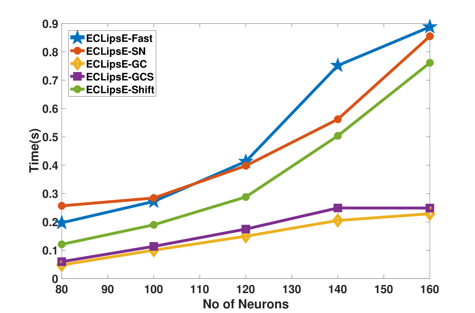
For deep neural networks, the computational time required to estimate the bounds is another crucial factor. Figure 1 presents a comparison of the computational time required by the proposed techniques as the number of neurons per layer increases from 80 to 160. Since ECLipsE-GC and ECLipsE-GCS replace the largest singular value computation with sum-based operators, they outperform ECLipsE-Fast in terms of computational efficiency. This demonstrates that these methods not only produce tighter Lipschitz bounds but also significantly reduce computational overhead, making them more suitable for large-scale neural networks.
V Conclusion
In this paper, we develop a family of new scalable Lipschitz bounds that do not require solving SDPs and can reduce the conservatism in the previous SOTA non-SDP bound ECLipsE-Fast. We provide a principled approach that leverages analytical solutions of a particular matrix inequality to streamline the developments of scalable Lipschitz bounds for deep networks. Our numerical results support our claim that our derived Lipschitz bounds are less conservative than ECLipsE-Fast while maintaining the same level of scalability.
References
- [1] Y. Tsuzuku, I. Sato, and M. Sugiyama, “Lipschitz-margin training: Scalable certification of perturbation invariance for deep neural networks,” Advances in Neural Information Processing Systems, 2018.
- [2] P. L. Bartlett, D. J. Foster, and M. J. Telgarsky, “Spectrally-normalized margin bounds for neural networks,” Advances in neural information processing systems, 2017.
- [3] M. Jin and J. Lavaei, “Stability-certified reinforcement learning: A control-theoretic perspective,” IEEE Access, vol. 8, pp. 229 086–229 100, 2020.
- [4] M. Fazlyab, M. Morari, and G. J. Pappas, “An introduction to neural network analysis via semidefinite programming,” in 2021 60th IEEE Conference on Decision and Control (CDC), 2021, pp. 6341–6350.
- [5] F. Fabiani and P. J. Goulart, “Reliably-stabilizing piecewise-affine neural network controllers,” IEEE Transactions on Automatic Control, vol. 68, no. 9, pp. 5201–5215, 2022.
- [6] A. Virmaux and K. Scaman, “Lipschitz regularity of deep neural networks: analysis and efficient estimation,” in Advances in Neural Information Processing Systems, 2018.
- [7] M. Fazlyab, A. Robey, H. Hassani, M. Morari, and G. Pappas, “Efficient and accurate estimation of Lipschitz constants for deep neural networks,” Advances in Neural Information Processing Systems, 2019.
- [8] P. Pauli, A. Koch, J. Berberich, P. Kohler, and F. Allgöwer, “Training robust neural networks using Lipschitz bounds,” IEEE Control Systems Letters, vol. 6, pp. 121–126, 2021.
- [9] P. Pauli, N. Funcke, D. Gramlich, M. A. Msalmi, and F. Allgöwer, “Neural network training under semidefinite constraints,” in IEEE Conference on Decision and Control (CDC), 2022, pp. 2731–2736.
- [10] M. Revay, R. Wang, and I. R. Manchester, “Lipschitz bounded equilibrium networks,” arXiv preprint arXiv:2010.01732, 2020.
- [11] A. Araujo, A. J. Havens, B. Delattre, A. Allauzen, and B. Hu, “A unified algebraic perspective on Lipschitz neural networks,” in International Conference on Learning Representations, 2023.
- [12] Z. Wang, G. Prakriya, and S. Jha, “A quantitative geometric approach to neural-network smoothness,” in Advances in Neural Information Processing Systems, 2022.
- [13] A. Havens, A. Araujo, S. Garg, F. Khorrami, and B. Hu, “Exploiting connections between Lipschitz structures for certifiably robust deep equilibrium models,” Advances in Neural Information Processing Systems, 2023.
- [14] P. Pauli, A. J. Havens, A. Araujo, S. Garg, F. Khorrami, F. Allgöwer, and B. Hu, “Novel quadratic constraints for extending lipsdp beyond slope-restricted activations,” in International Conference on Learning Representations, 2024.
- [15] N. H. Barbara, R. Wang, and I. R. Manchester, “On robust reinforcement learning with Lipschitz-bounded policy networks,” arXiv preprint arXiv:2405.11432, 2024.
- [16] R. Wang and I. Manchester, “Direct parameterization of lipschitz-bounded deep networks,” in International Conference on Machine Learning, 2023.
- [17] A. Xue, L. Lindemann, A. Robey, H. Hassani, G. J. Pappas, and R. Alur, “Chordal sparsity for lipschitz constant estimation of deep neural networks,” in 2022 IEEE 61st Conference on Decision and Control (CDC), 2022, pp. 3389–3396.
- [18] P. Pauli, D. Gramlich, and F. Allgöwer, “Lipschitz constant estimation for 1d convolutional neural networks,” in Learning for Dynamics and Control Conference, 2023, pp. 1321–1332.
- [19] Z. Wang, B. Hu, A. J. Havens, A. Araujo, Y. Zheng, Y. Chen, and S. Jha, “On the scalability and memory efficiency of semidefinite programs for Lipschitz constant estimation of neural networks,” in International Conference on Learning Representations, 2024.
- [20] P. Pauli, D. Gramlich, and F. Allgöwer, “Lipschitz constant estimation for general neural network architectures using control tools,” arXiv preprint arXiv:2405.01125, 2024.
- [21] Y. Xu and S. Sivaranjani, “Eclipse: Efficient compositional lipschitz constant estimation for deep neural networks,” in The Thirty-eighth Annual Conference on Neural Information Processing Systems, 2024.
- [22] C. Szegedy, W. Zaremba, I. Sutskever, J. Bruna, D. Erhan, I. Goodfellow, and R. Fergus, “Intriguing properties of neural networks,” in International Conference on Learning Representations, 2014.
- [23] R. Horn and C. Johnson, Matrix Analysis. Cambridge University Press, 2012.
- [24] B. Delattre, Q. Barthélemy, A. Araujo, and A. Allauzen, “Efficient bound of lipschitz constant for convolutional layers by gram iteration,” in International Conference on Machine Learning, 2023.
- [25] E. Grishina, M. Gorbunov, and M. Rakhuba, “Tight and efficient upper bound on spectral norm of convolutional layers,” in European Conference on Computer Vision, 2024, pp. 19–34.