Entente: Cross-silo Intrusion Detection on Network Log Graphs
with Federated Learning

Abstract.

Graph-based Network Intrusion Detection System (GNIDS) has gained significant momentum in detecting sophisticated cyber-attacks, like Advanced Persistent Threat (APT), in an organization or across organizations. Though achieving satisfying detection accuracy and adapting to ever-changing attacks and normal patterns, all prior GNIDSs assume the centralized data settings directly, but non-trivial data collection is not always practical under privacy regulations nowadays. We argue that training a GNIDS model has to consider privacy regulations, and propose to leverage federated learning (FL) to address this prominent challenge.

Yet, directly applying FL to GNIDS is unlikely to succeed, due to issues like non-IID (independent and identically distributed) graph data over clients and the diverse design choices taken by different GNIDS. We address these issues with a set of novel techniques tailored to the graph datasets, including reference graph synthesis, graph sketching and adaptive contribution scaling, and develop a new system Entente. We evaluate Entente on the large-scale LANL, OpTC and Pivoting datasets. The result shows Entente outperforms the other baseline FL algorithms and sometimes even the non-FL GNIDS. We also evaluate Entente under FL poisoning attacks tailored to the GNIDS setting, and show Entente is able to bound the attack success rate to low values. Overall, our result suggests building cross-silo GNIDS is feasible and we hope to encourage more efforts in this direction.

1. Introduction

The techniques and scale of modern cyber-attacks are evolving at a rapid pace. More high-profile security breaches are observed against large organizations nowadays. One prominent attack strategy is Advanced Persistent Threat (APT) (Lockheed Martin, 2019), which establishes multiple attack stages and infiltrates multiple organizational assets through techniques like lateral movement. As a popular countermeasure, many organizations collect network logs (e.g., firewall and proxy logs) and perform intrusion detection on them (Li and Oprea, 2016). To more precisely capture the distinctive network communication patterns of the attack, a promising approach is to model the network logs as graph and apply graph-based algorithms to detect abnormal entities, interactions or communities. We term such system Graph-based Network Intrusion Detection System (GNIDS), and we observe that the recent works (Xu et al., 2024; King and Huang, 2023; Khoury et al., 2024; Paudel and Huang, 2022; Liu et al., 2019; Bowman et al., 2020; Cheng et al., 2021; Sun and Yang, 2022; Rabbani et al., 2024; Qiu et al., 2023) prefer advanced graphical models like graph autoencoder (GAE) (Kipf and Welling, 2016b) to build their systems, showing much higher detection accuracy over the traditional NIDS and capabilities of detecting sophisticated attacks like lateral movement (Khoury et al., 2024).

Regulation compliance concerns for GNIDS. Given the sensitive nature of network logs—such as revealing communication patterns of employees and organizations (Imana et al., 2021)—privacy regulations present significant compliance concerns when training GNIDS models with logs from multiple regions. Recent discussions have highlighted the challenges data privacy regulations pose to cybersecurity systems like security information and event management (SIEM) (Menges et al., 2021). For example, Menges et al. advocate SIEM to be compliant with Europe’s General Data Protection Regulation (GDPR) (Menges et al., 2021), which covers the data processing and transfer “within and between private companies and/or public bodies in the European member states”. Outside Europe, regional regulations add further complexity: for example, Singapore’s Personal Data Protection Act (PDPA) prohibits using data for purposes beyond its original intent without explicit individual consent (Lim, 2023), creating barriers for training security models on network logs. The deployment of GNIDS requires analyzing interactions across organizations or departments, but centralized log-based training may be infeasible due to privacy restrictions. To address these regulation compliance concerns, there is an urgent need for a new framework that aligns with diverse privacy laws.

Federated Learning for GNIDS. To address the privacy issues in other domains, e.g., training an image classifier over people’s images, Federated Learning (FL) has been proposed and gained prominent attraction from the academia and industry (Yang et al., 2019). In essence, FL allows the individual data owners (e.g., a device owner or an organization) to keep their data in premise and jointly train a global model. Recently, some works have applied FL to train models for security applications (Fereidooni et al., 2022; Ongun et al., 2022; Rey et al., 2022; De La Torre Parra et al., 2022; Naseri et al., 2022), but we found none of the prior works apply to GNIDS. We believe FL is a reasonable solution to address the aforementioned privacy issues GNIDS because 1) the long trajectory of the contemporary cyber-attacks (e.g., traversing through different departments and organizations (Lockheed Martin, 2019)) underscores the importance of multi-region logs and 2) FL exchanges model parameters instead of raw data. Hence, we pivot the research of developing a practical FL-powered GNIDS and term our new system Entente.

Design of Entente. We argue that Entente should satisfy three critical design goals: effectiveness (similar effectiveness as the GNIDS trained on the entire dataset), scalability (the overhead introduced by the FL mechanism should be small and a large number of FL clients should be supported) and robustness (maintaining detection accuracy against attackers who compromise the FL procedure). Yet, based on our survey, none of the existing FL methods are able to achieve these goals altogether. In addition, the data to be processed by GNIDS usually have imbalanced classes (e.g., malicious events are far less than the normal events) and non-IID (not independent and identically distributed) across FL clients, which is a well-known challenge to FL (Li et al., 2019; Hsu et al., 2019).

We address these issues by leveraging the domain knowledge of GNIDS and its data, and design a new FL protocol that achieves effectiveness, scalability and robustness goals altogether. To address the issues of class imbalance and non-IID, we observe that clients’ initial weights play a critical role, and it can be instantiated with help of the parameter server without leaking clients’ statistics. We develop a new FL bootstrapping protocol based on reference graph synthesis and graph sketching, which only involve lightweight computation on the parameter server and FL clients, and a new technique termed adaptive contribution scaling (ACS) to adjust the clients’ weights dynamically in each round. Second, the attacker needs to scale up the model updates to effectively poison the trained global model. Since the clients weights are adjusted under ACS already, we can bound the model updates by tweaking ACS. We are also able to formally prove the convergence rate is bounded, suggesting it could be useful for other applications under federated graph learning. Finally, though the design choices of existing GNIDSs are vastly different, we found there exists a unified workflow and their trainable components can be updated concurrently within each FL iteration. We adapt the classic FedAvg algorithm (McMahan et al., 2017), which is compatible with the existing GNIDS paradigms, and develop Entente on top of it.

Evaluation of Entente. We conduct an extensive evaluation on Entente, focusing on its effectiveness of detecting abnormal interactions between entities. We adapt Entente to two exemplar GNIDS, namely Euler (King and Huang, 2023) and Jbeil (Khoury et al., 2024), as they embody quite different designs. We choose three real-world large-scale log datasets, OpTC (Five Directions, 2020), LANL Cyber1 (or LANL) (Kent, 2015) and Pivoting (Apruzzese et al., 2017) for evaluation. Different client numbers are simulated. On OpTC, Entente outperforms all the other baseline FL methods and even the non-FL version (the GNIDS is trained using all data) with over 0.1 increase of average precision (AP). On LANL and Pivoting, when link prediction is conducted by Jbeil, high AP and AUC can be reached by Entente (over 0.9 in most cases), for both transductive learning and inductive learning modes. On LANL when Euler is used, given only hundreds of redteam events are used for edge classification, the AP is low for all FL methods, but Entente still outperforms the other methods in most cases.

We also consider the robustness of Entente under adaptive attacks and consider model poisoning (Bagdasaryan et al., 2020) as the main threat. We adapt the attack that scales up the model updates(Bagdasaryan et al., 2020) and adds covering edges (Xu et al., 2023) to the GNIDS setting, by replaying malicious edges from the testing period to the training period. Since Entente integrates norm bounding when adjusting clients’ weights, the attack success rate is bounded to a very low rate, e.g., less than 10% when attacking Euler+LANL. Without norm bounding, not only attack success rate increases, the FL training process might not even finish when the attacker scales the model updates by a very large ratio.

Overall, our study shows promises in addressing the data sharing concerns in building GNIDS in practice.

Contributions. We summarize the contributions of this paper as follows:

• We propose a new system Entente that can train a GNIDS model without requesting data sharing among departments/ organizations, under the framework of FL.

• We address the threats like non-iid client graphs and adaptive attackers with novel techniques like reference graph synthesis and adaptive contribution scaling. We also formally prove our method has bounded convergence rate.

• We conduct the extensive evaluation using large-scale log datasets (LANL, OpTC and Pivoting), and the result shows Entente can outperform other baselines in most cases.

2. Background

2.1. Graph-based Network Intrusion Detection Systems (GNIDS)

Network logs collected by network appliances like firewall and proxy have been extensively leveraged to detect various cyber-attacks, including APT attacks (Lockheed Martin, 2019). Many graph-based approaches have been developed in recent years and we term them Graph-based Network Intrusion Detection Systems (GNIDS). At the high level, for each log entry, the GNIDS extracts the subject and object fields (e.g., host) as nodes, and fills the edge attributes using the other fields (e.g., the instruction contained in the network packet). In Figure 1, we illustrate an example of a graphs generated from network logs collected by different organizations (or clients).

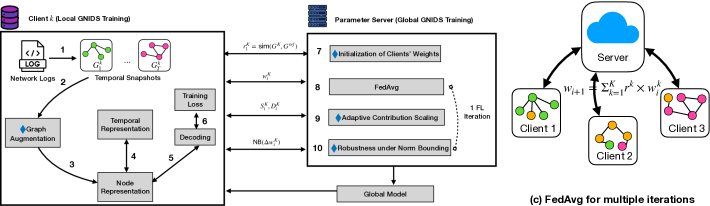
Figure 1. An example summarized from the day 1 attack campaign in the OpTC dataset (Five Directions, 2020). The attacker firstly connects to machine0201 and downloads the powershell attack tool. Then it pivots to machine machine0401 and machine0660 with Windows WMI command. Finally, the attack spreads to other machines. The attacked machines can belong to multiple organizations (or clients). Graphs can be constructed separately from the logs collected by different clients.

On top of the graph data, GNIDS can perform anomaly detection with a trained model. The relevant works can be divided by their classification targets: sub-graphs (e.g., a graph snapshot), nodes (e.g., a host) and edges (e.g., interactions between hosts). In order to accurately model the patterns in the graph data, most works choose Graph Neural Network (GNN). One prominent technique is graph autoencoder (GAE) (Kipf and Welling, 2016b), which uses a graph encoder to generate node embedding and a graph decoder to reconstruct a similar graph. The downstream tasks like edge classification can be done by generating edge scores from node embedding and comparing them with a threshold. In Section 4, we elaborate the common design choices of GNIDS models when describing the workflow of Entente.

Noticeably, a relevant line of research is provenance- or host-based intrusion detection system (PIDS or HIDS) (Zipperle et al., 2022; Inam et al., 2023), which detects intrusions on the host log graph. In Section 7, we discuss this line and the potential changes of our system Entente for adaption.

2.2. Federated Learning

Federated Learning (FL) is an emerging technique to allow multiple clients to train a model without revealing their private data (Konečnỳ et al., 2016; McMahan et al., 2017). FL relies on a central parameter server to train a global model under multiple iterations. At the start of each iteration $i$, the server transmits a global model ($w_{i}$) to a set of clients ($1,\dots,K$) and they train local models ($w_{i}^{1},\dots,w_{i}^{K}$) from $w_{i}$. Then the clients transmit the local models to the server to average their differences (e.g., FedAVG on model parameters (McMahan et al., 2017)) and generate a new $w_{i+1}$.

FL has two main deployment settings: horizontal FL and vertical FL (Yang et al., 2019). For horizontal FL, the clients’ datasets have a large overlap in the same feature space but little overlap in the sample space (e.g., every client owns the same type of network logs of its sub-network machines). On the contrary, vertical FL assumes the clients have a large overlap in the sample space but little overlap in the feature space (e.g., each client collects a unique type of logs for all organizational machines). In this work, we focus on horizontal FL, which has been studied more often (Yang et al., 2019). We also focus on the cross-silo FL setting, in which a small number of organizations participate in the entire training process (Huang et al., 2022), rather than cross-device FL setting, in which many user-owned devices selectively participate in different training iterations.

Federated Graph Learning (FGL). Initially, FL was developed for tasks related to Euclidean data like image classification (McMahan et al., 2017). Recently, FL has been applied to non-Euclidean data like graphs (Liu et al., 2022; Fu et al., 2022), and these works are termed under Federated Graph Learning (FGL). Under the horizontal FL setting, the graph data is partitioned across clients, where each client has a sub-graph with non-overlapping (or little overlapping) nodes. A prominent challenge for sub-graph FL is the heterogeneity between clients’ subgraphs, such that the sizes and topology are vastly different between subgraphs. While there are general solutions to address the data heterogeneity issues under FL (Reddi et al., 2020; Li et al., 2020a), some solutions are customized to sub-graph FL (Li et al., 2023a; Wang et al., 2024). For example, FedGTA proposed a topology-aware optimization strategy for FGL (Li et al., 2023a), but it requires heavy changes on the design of existing graphical models.

Alternatively, some works propose to amend each subgraph with some information shared by other clients or server (Zhang et al., 2021b; Chen et al., 2021; Zhang et al., 2021a; Peng et al., 2022; Zhu et al., 2024). For example, the server in FedGL asks the clients to upload node embeddings to generate a global pseudo embedding (Chen et al., 2021). FedSage+ asks the clients to train a neighborhood generator jointly (Zhang et al., 2021a). However, there is no guarantee that the shared information will not leak more clients’ information (e.g., node embedding can lead to inference attacks (Zhang et al., 2022a)). To mitigate the privacy concerns, cryptographic primitives and/or differential privacy have been tested to amend the subgraph in a privacy-preserving way (Yao et al., 2022; Zhang et al., 2021a; Qiu et al., 2022; Wu et al., 2021). For example, FedGCN allows a client to collect 1-hop or 2-hop averaged neighbor node features from clients with Fully Homomorphic Encryption (FHE) (Yao et al., 2022). However, significant computation and communication overhead will be incurred.

In this work, we develop a new FGL technique to tackle the subgraph heterogeneity issue and apply FL to GNIDS in practice.

3. Overview

In this section, we first describe the deployment settings of our system Entente. Then, we demonstrate the goals to be achieved by Entente. Finally, we describe the threat model.

3.1. Deployment Settings

We assume an organization consists of multiple sub-organizations, but it is not always feasible for them to share the raw logs with each other, e.g., when they are located in disjoint regions that are governed by privacy laws like GDPR, as elaborated in Section 1. Each sub-organization collects the logs about the network packets sent to and received by its controlled machines, with systems like SIEM (IBM, 2023), and trains a local GNIDS model to detect past or ongoing attacks by analyzing the logs. To achieve better detection coverage and effectiveness, they decide to perform FL to jointly train a global GNIDS model that can be used by each participated sub-organization. The same procedure can be taken by multiple independent organizations to train a global GNIDS model.

Here we formally define the entities that deploy our system. Figure 1 also illustrates the setup.

• A client is the sub-organization that collects logs from its managed machines and trains a GNIDS model to perform intrusion detection.

• A parameter server is operated by an entity outside the clients (e.g., the parent organization of the clients) to aggregate the clients’ model updates and pushes the global model to clients.

• A machine owned by a client is subjected to attacks. It produces network logs that are collected by the client. Each machine is also called a node under the client graph.

3.2. Design Goals and Challenges

When designing Entente, we identify several goals that should be achieved to enable its real-world deployment.

• Effectiveness. Entente should achieve high detection accuracy and precision on large-scale real-world logs. Achieving high precision is more important due to the imbalanced data distribution in the log dataset (Quiring et al., 2022). Entente should achieve comparable effectiveness as the GNIDS trained on the entire log dataset.

• Scalability. The introduced FL mechanisms should be scalable when training a global model from large-scale log datasets owned by many clients. The communication overhead and latency added by Entente on each client should be small.

• Robustness. In addition to compromising the client machines, the attacker has motivation to compromise the FL procedure. Entente should be able to defend against such adaptive attack.

Challenges. The major challenge is the heterogeneity among clients. Previous studies have discovered that when clients’ data are non-IID (independent and identically distributed), the effectiveness and robustness of the trained global model can be significantly degraded (Li et al., 2019). In our case, it is very likely that each client has very different subgraphs in terms of size and topology. As supporting evidence, Dambra et al. studied the malware encounters using the telemetry data from a security company, and it shows enterprises in the United States have more than 5x monitored end-hosts than any other country (Dambra et al., 2023). In Table 12, we show our datasets have this problem.

Second, due to the scalability requirement listed above, prior approaches that address client heterogeneity with heavyweight cryptographic methods, as reviewed in Section 2.2, are not suitable. In addition, achieving FL robustness under non-iid datasets is challenging due to the divergence of normal model updates.

Third, GNIDS could be executed under different graph modeling (e.g., static graph and temporal graph), downstream tasks (e.g., edge and node classification) and training/testing setup (e.g., transductive learning and inductive learning). A GNIDS trained under FL that achieves satisfactory performance in all these settings requires careful design.

3.3. Threat Model

Firstly, we consider the attackers that compromise machines of a client. We follow the threat model of the other GNIDS (e.g.,  (King and Huang, 2023; Khoury et al., 2024)) that assume though the machines can be compromised, the network communications are correctly logged by the network appliances. Hence, log integrity can be achieved. Though it is possible that advanced attackers could violate this assumption, additional defenses (e.g., using Trusted Execution Environment) can be deployed as a countermeasure (Bates et al., 2015; Paccagnella et al., 2020; Gandhi et al., 2023).

Secondly, we consider the attackers compromise the FL process and are able to launch the poisoning attack, which is the major threat against FL. We assume some of the participated clients are subject to data poisoning (Bagdasaryan et al., 2020) (e.g., the adversary commands some compromised machines to initiate covering communications during the training stage) or model poisoning (Bagdasaryan et al., 2020) (e.g., the adversary manipulates the updates of local models). In Section 5.4, we introduce a concrete attack against GNIDS in the FL setting, and demonstrate Entente is an effective defense.

Finally, we follow the threat model as the basic FedAvg method that assumes the central data collector is interested in inferring the sensitive information (e.g., communications between two employees of a sub-organization). The raw logs remain local to each FL client, and only the model updates are transmitted to the parameter server. To mitigate privacy leakage, we only allow the parameter server to know the total number of nodes aggregated from all clients. Yet, the node number from each client is not necessarily known. We argue the total node number is usually not a secret in an organization, as explained in Section 4.3. In Section 6, we further discuss the privacy implications of our deployment settings and provide preliminary analysis under the lenses of differential privacy (DP).

4. Design of Entente

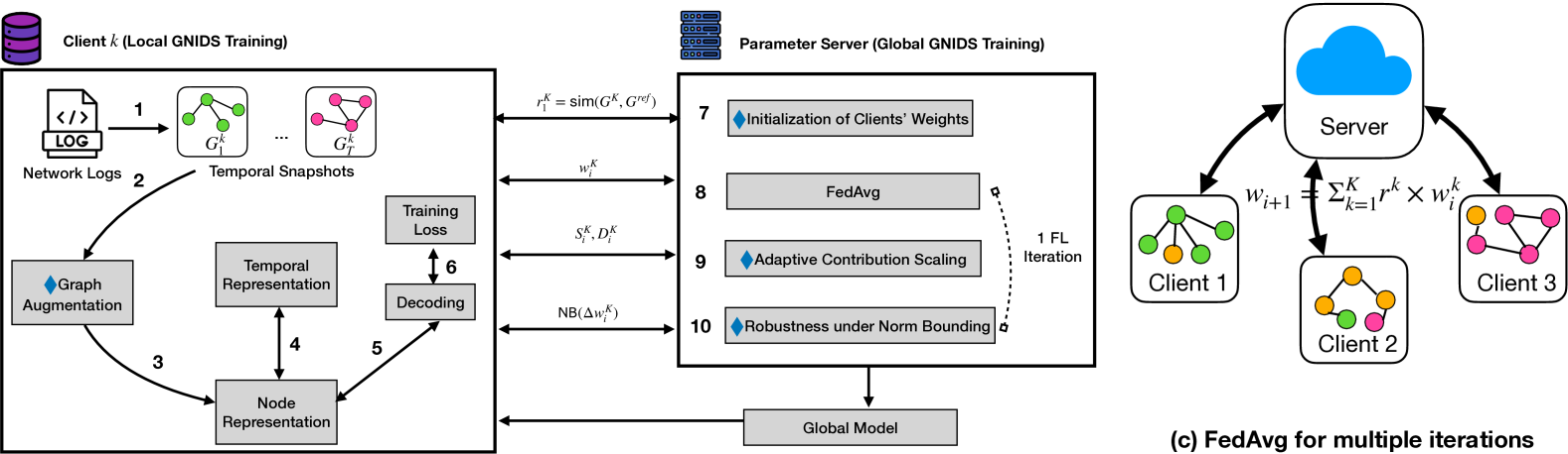
Figure 2. The workflow of Entente. The client $k$ trains a GNIDS model locally and communicates with the parameter server to jointly learn a global GNIDS with other clients. Function Sim computes graph similarity.

In this section, we describe Entente in detail. Entente encompasses GNIDS components that are adapted from the existing works and FL components that train the GNIDS models. We highlight FL-related components with “$\blacklozenge$” as they are the key contributions of this work. The high-level workflow of Entente is illustrated in Figure 2. The mainly used symbols and their meanings are summarized in Table 1.

Table 1. The main symbols used in the paper.

Term(s)	Symbol(s)
Client number, index	$K$, $k$
Client graph	$\mathcal{G}^{k}$
Client edges, edge	$\mathcal{E}^{k}$, $e^{k}$
Client nodes, node	$\mathcal{V}^{k}$, $v^{k}$
Snapshot number, index	$T$, $t$
Client snapshot	$\mathcal{G}^{k}_{t}$
Client model parameters	$w^{k}$
FL max and current iteration	$R$, $i$
Weight of a client update	$r^{k}$
Global model after $i$ iterations	$w_{i+1}$

4.1. Local Graph Creation

We assume $K$ clients have deployed the same GNIDS and they jointly train a global model with FL. Each client is indexed by $k\in[1,K]$. After the network logs are collected by client $k$, a graph $\mathcal{G}^{k}$ will be constructed by representing the event sources and destinations (machines/users/etc.) as nodes $\mathcal{V}^{k}$ and their communications as edges $\mathcal{E}^{k}$. An edge $e^{k}$ between a pair of nodes $v^{k}_{1}$ and $v^{k}_{2}$ could contain features extracted from one or many events that have both $v^{k}_{1}$ and $v^{k}_{2}$, and the commonly used features include the event frequency (King and Huang, 2023), traffic volume of network flows (Xu et al., 2024), etc. Each node has a feature vector, which can be the node type (e.g., workstation or server), privilege, etc. (King and Huang, 2023)

Though it is relatively straightforward to generate a single static graph from all events (Zeng et al., 2022), such graph modeling has prominent issues like the coarse detection granularity and missing the unique temporal patterns (Xu et al., 2024). Recent works advocate dynamic graph modeling that generate a sequence of temporal snapshots $[\mathcal{G}_{1},\cdots,$ $\mathcal{G}_{T}]$, and a snapshot $\mathcal{G}_{t}$ ($t\in[1,T]$) merges the events in a fix-duration time window (e.g., one hour) (Xu et al., 2024; King and Huang, 2023; Khoury et al., 2024). Entente generates dynamic graph by default, but it can easily be switched to the static modeling by merging the nodes and edges of $[\mathcal{G}^{k}_{1},\cdots,\mathcal{G}^{k}_{T}]$, yielding $\mathcal{G}^{k}$.

$\blacklozenge$Augmenting local graph. Missing cross-client edges is a prominent issue for subgraph FL, and previous works tried to amend the subgraph by exchanging the topological information among clients, which however lead to privacy and efficiency issues, as surveyed in Section 2.2. We found this problem can be partially addressed under the unique GNIDS deployment setting, with 1-hop graph augmentation. Our key insight is that the log collectors deployed by a client, like firewalls, usually record the inbound and outbound cross-client events automatically (Li and Oprea, 2016). Therefore, the cross-client edges can be harvested “for free” from each client’s internal logs.

Specifically, assume $\mathcal{V}_{t}^{k}$ and $\mathcal{E}_{t}^{k}$ are nodes and edges of the snapshot $\mathcal{G}_{t}^{k}$ of client $k$. We search the logs to find all entities that are not contained by $\mathcal{V}_{t}^{k}$ while following the constraints of $\mathcal{V}_{t}^{k}$ (e.g., in the same snapshot period), denoted as $\mathcal{V}_{t}^{k\complement}$. Then $\mathcal{V}_{t}^{k\complement}$ will be added into $\mathcal{G}_{t}^{k}$, together with $\mathcal{E}_{t}^{k\complement}$ (the edges between $\mathcal{V}_{t}^{k}$ and $\mathcal{V}_{t}^{k\complement}$).

4.2. Local GNIDS Training

Node representation learning. On a generated graph snapshot $\mathcal{G}^{k}_{t}$, Entente extracts the representation (or embedding) of each node with a graph auto-encoder (GAE) (Kipf and Welling, 2016b), which aggregates the node’s features and its neighborhood information. Graph Convolutional Network (GCN) (Kipf and Welling, 2016a) is a standard choice (King and Huang, 2023), which takes the whole adjacency matrix as the input, but only transductive learning, which assumes the nodes are identical between training and testing, is supported. In our setting, the GCN encoder can be written as:

(1) $$Z^{k}_{t}=\text{GCN}(X^{k}_{t},A^{k}_{t})$$

where $Z^{k}_{t}\in\mathbb{R}^{n\times r}$ is the node embedding generated by the encoder on $\mathcal{G}^{k}_{t}$, $X^{k}_{t}$ represents the node features and $A^{k}_{t}$ represents the adjacency matrix on $\mathcal{G}^{k}_{t}$.

To accommodate the new nodes observed in the testing phase, inductive learning has been proposed, which learns the neighborhood aggregator to generate node embedding. GraphSage (Hamilton et al., 2017) is a classic encoder in this case, but recent GNIDS (Khoury et al., 2024) also integrate the other encoders like Temporal Graph Networks (TGN) (Rossi et al., 2020). The TGN encoder deals with continuous-time dynamic graph, and for each time $t$, the node embedding $Z^{k}_{t}$ is generated by trainable message function, message aggregator and memory updater.

Temporal learning. The anomalous temporal patterns (e.g., a login attempt outside of work hours) provides important indicators for intrusion detection, and some recent GNIDS (King and Huang, 2023; Xu et al., 2024) choose to capture such patterns with Recurrent Neural Network (RNN), e.g., Gated Recurrent Unit (GRU) under RNN families. The RNN module can be written as:

(2) $$[Z^{k}_{1},\dots,Z^{k}_{T}]=\text{RNN}([\text{ENC}(\mathcal{G}^{k}_{1}),\dots,\text{ENC}(\mathcal{G}^{k}_{T})])$$

where $\mathcal{G}^{k}_{t}=(X^{k}_{t},A^{k}_{t})$ ($t\in[1,T]$) , ENC is the encoder (e.g., GCN), and $[Z^{k}_{1},\dots,Z^{k}_{T}]$ are the embeddings updated by RNN after they are encoded from $[\mathcal{G}^{k}_{1},\dots,\mathcal{G}^{k}_{T}]$.

When TGN is the encoder, the temporal pattern is directly handled by its memory module, which can be vanilla RNN and GRU (Rossi et al., 2020). Hence, no extra RNN layer is needed.

Both GCN+RNN and TGN encoders (and other encoders used by GNIDS) are supported by Entente when they are trained under FL and we explain this feature in Section 4.3.

Decoding. On the node representations, the decoder aims to reconstruct the adjacency matrix with edge scores. The basic decoder is inner product decoder (King and Huang, 2023), which can be written as:

(3) $$\text{DEC}(Z^{k}_{t})=\Pr(A^{k}_{t+n}=1|Z^{k}_{t})=\sigma(Z^{k}_{t}Z_{t}^{k\intercal})$$

where $\sigma(\cdot)$ is the logistic sigmoid function and $\Pr(A_{t+n}=1|Z_{t})$ is the reconstructed adjacency matrix at time $t+n$ given $Z_{t}$. The probability at each matrix cell is used as an edge score.

The simplicity of the inner product could lead to prominent reconstruction loss, and more complex, trainable decoders like Multilayer Perceptron (MLP) have been used by GNIDS (Xu et al., 2024; Khoury et al., 2024). We design Entente to support different variations of decoders as elaborated in Section 4.3.

Training loss. When training a GNIDS, the weights of trainable components, including graph encoder, RNN and decoder, are updated under a loss function. The typical choice is cross-entropy loss, which can be written as:

(4) $$\mathcal{L}=-\log(\Pr(A^{k}_{t}|\hat{A^{k}_{t}}))$$

where $\hat{A^{k}_{t}}$ is the adjacency matrix decoded from node embeddings.

When the GNIDS is trained with only benign events in unsupervised learning mode, negative sampling (Mikolov et al., 2013) can be applied to randomly select non-existent data points as the malicious samples (e.g., non-existent edges (King and Huang, 2023; Xu et al., 2024)).

4.3. Federated GNIDS Training

We aim to support different GNIDS graph modeling, downstream tasks, training/testing setup, as described in Section 3.2. Hence, Entente is designed to augment the existing GNIDS without heavy adjustment of their components, and the FGL works that redesign the local models (Meng et al., 2021; Li et al., 2023a) are not suitable. Based on our survey of existing FL frameworks, we are motivated to build Entente on top of FedAVG, because 1) it only needs clients’ model parameters as input, and 2) it has demonstrated effectiveness when the clients’ models are GNN (Wang et al., 2022) and RNN (Hard et al., 2018). Since the common GNIDS components like node representation learning, temporal learning and decoding all use the same set of training data, we could train them independently with FedAvg and update their model parameters. As such, Entente not only incurs minimum development overhead, but also achieves similar or even better effectiveness comparing to the original GNIDS, as supported by the evaluation (Section 5). We also want to point out the standard FedAvg workflow leads to unsatisfactory performance and we elaborate the key adjustment below.

$\blacklozenge$Initialization of clients’ weights. FedAVG aggregates the model parameters of GNIDS components in a number of iterations as described in Section 2.2. Its basic version in one iteration can be represented as:

(5) $$w_{i+1}=\Sigma^{K}_{k=1}r^{k}\times w^{k}_{i}$$

where $i$ is the current iteration, $w^{k}_{i}$ is the local model parameters of client $C_{k}$ that is trained with the global model of previous iteration $w_{i}$ and its local data, $r^{k}$ is the weight of client $k$ during aggregation, and $w_{i+1}$ is the global model parameters after aggregation. As described in Section 3.2, the clients’ data are non-IID, which has a prominent impact on the performance of FL algorithms. To tackle non-IID data, one feasible approach is to assign different weights to the model updates from different clients, so the impact from clients with outlying distribution can be contained. Previous works have used the number of data samples (e.g., images (McMahan et al., 2017)) per client for weights, but in our case, each client only has one sub-graph.

We address this challenge with a new method to initialize the client’s weights based on its graph properties. We minimize the communication overhead and privacy leakage by computing the client’s weights on top of a single reference graph generated by the parameter server. This reference graph stays the same for the whole training process and across clients. Our approach is inspired by Zhao et al., which distributes a warm-up model trained with globally shared data and shows test accuracy can be increased (Zhao et al., 2018).

Specifically, we assume the server knows the total number of nodes ($n$) from all clients. We argue this information is often accessible within an organization (e.g., an administrator can get the list of users from active directory (Microsoft, 2023)), so no extra privacy leakage is expected. When bootstrapping FL, the parameter server generates a reference graph $\mathcal{G}^{ref}$ and distributes it to all clients for them to compute $r^{k}$ ($\forall k\in[1,K]$). We choose to apply Barabási–Albert (BA) Model (Barabási and Albert, 1999) to generate the reference graph. BA model is a random graph model for complex networks analysis (Drobyshevskiy and Turdakov, 2019), and it is selected

because 1) it only needs the number of nodes ($n$) and the number of initial edges for a new node ($m$) and 2) it has low computational overhead (complexity is $O(n\times m)$) when $m$ is small. In Section 5.1 and Appendix 5.5, we discuss the selection of $m$ and evaluate its impact. The pseudo-code of BA model is written in Appendix A.

On a client $C^{k}$, $r^{k}$ will be initialized based on the graph similarity between its generated graph $\mathcal{G}^{k}$ (aggregated from $[\mathcal{G}_{1}^{k},\dots,\mathcal{G}_{T}^{k}]$) and $\mathcal{G}^{ref}$. Intuitively, the client with a similar distribution to the global data should receive high $r^{k}$. Noticeably, we compute $r^{k}$ locally on the client, so nothing about the client’s data or distribution will be learned by the server. This is different from the standard FedAVG which computes weights on the server. However, graph similarity is computationally intensive: e.g., graph edit distance (GED) is a fundamental NP-hard problem (Bunke, 1997). Therefore, we choose to compute the similarity on the graph sketches instead of raw graphs for efficiency. We use Weisfeiler-Lehman (WL) graph kernel (Shervashidze et al., 2011) to capture the graph structure surrounding each node and compute histogram by nodes’ neighborhood.

Data: Graph $\mathcal{G}$

Result: histograms

$\text{labels}\leftarrow\text{InitializeLabels}(\mathcal{G})$;

$\text{histograms}\leftarrow\text{Histogram}(\text{labels})$;

for $i=1$ to MaxIters do

    foreach $v$ in $\mathcal{G}$ do

       $\text{neigh}\leftarrow\text{NeighborLabels}(v,\text{labels})$;

       $\text{labels}[v]\leftarrow\text{Hash}(\text{Sort}(\text{labels}[v]+\text{neigh}))$;

      

   $\text{histograms}\leftarrow\text{Append}(\text{histograms},\text{Histogram}(\text{labels}))$

   

return histograms

Algorithm 1 Weisfeiler-Lehman Histogram (WLH).

In Algorithm 1, we describe how to compute the Weisfeiler-Lehman histogram (WLH), where InitializeLabels assigns node degree as a label to each node $v$, NeighborLabels creates a multiset containing $v$’s current label and its neighbors’ labels, Hash and Sort produce a new label for $v$. $MaxIters$ is the number of iterations, and $i$th-iteration computes WLH for $i$-hop neighborhood. We set $MaxIters$ to 3. When applying Algorithm 1 to our setting, we compute the Jaccard similarity $S_{\mathsf{Jac}}^{k}$ between $\mathcal{G}^{k}$ and $\mathcal{G}^{ref}$.

(6) $$S_{\mathsf{Jac}}^{k}=\frac{\mathcal{G}^{ref}\cap\mathcal{G}^{k}}{\mathcal{G}^{ref}\cup\mathcal{G}^{k}}$$

$\blacklozenge$Adaptive contribution scaling (ACS). We follow the FedAVG client-server protocol to update the model parameters by iterations. While FedAvg uses the same $r^{k}$ throughout FL, we found the client contributions can be more precisely modeled by dynamically adjusting them towards stability. This idea at the high level has been examined by prior works like  (Siomos and Passerat-Palmbach, 2023; Wu and Wang, 2021; Cao et al., 2021), but we found none of them are suitable under our setting. First, they require the statistical information of local data (e.g., local gradients or local samples (Wu and Wang, 2021; Cao et al., 2021)), which has been avoid by Entente due to privacy concerns. Second, the contribution evaluation can be heavy (e.g., Shapley value by  (Siomos and Passerat-Palmbach, 2023)).

Instead, we propose a lightweight and privacy-preserving method termed adaptive contribution scaling (ACS) to adjust clients’ weights only using the model parameters. Specifically, for client $C^{k}$ at the FL iteration $i$, the parameter server computes a similarity metric $S^{k}_{i}$ based on the cosine similarity and a distance metric based on L2 distance $D^{k}_{i}$. The new client’ weights $r^{k}_{i}$ will be computed with $S_{\mathsf{Jac}}^{k}$, $S^{k}_{i}$ and $D^{k}_{i}$. $r^{k}_{1}$ is initialized using $S_{\mathsf{Jac}}^{k}$. ACS models both representational similarity (with $S^{k}_{i}$) and distance of local models to the global models (with $D^{k}_{i}$), hence presenting a more reliable indicator for client contributions. To mitigate model collapse incurred by some clients, the server bounds $D^{k}_{i}$ by a hyper-parameter $\omega$.

The definitions of $S^{k}_{i}$ and $D^{k}_{i}$, and the new aggregation function are listed below.

(7) $$S^{k}_{i}=\frac{||\sum w^{k}_{i}\times w_{i-1}||}{||\sum w_{i}^{k}||\times||w_{i-1}||}$$

(8) $$D^{k}_{i}=\frac{\omega\sqrt{\sum(w_{i}^{k}-w_{i-1})^{2}}}{\max(\omega,\sqrt{\sum(w_{i}^{k}-w_{i-1})^{2}})},\forall\omega>0$$

(9) $$w_{i+1}=\frac{1}{K}\sum^{K}_{k=1}r^{k}_{i}\times w^{k}_{i}\quad\mathrm{s.t.}\ r^{k}_{i}=c_{1}\times S_{\mathsf{Jac}}^{k}+c_{2}\times S^{k}_{i}\times D^{k}_{i}$$

where $c_{1}$ and $c_{2}$ are two constants to adjust the contributions from $S_{\mathsf{Jac}}^{k}$, $S^{k}_{i}$ and $D^{k}_{i}$.

With ACS, Entente is able to achieve better effectiveness in the evaluation. Moreover, we are able to formally prove that the iteration-wise difference shifting under Equation 9 is bounded, by $|\frac{w_{i+1}}{\sum_{k}w^{k}_{i}}|\leq c_{1}+c_{2}\omega$ from $\sum_{k}w^{k}_{i}$ (FedAVG).

Theorem 1.

Define $S_{\mathsf{Jac}}^{k},S^{k}_{i}$, and $D_{i}^{k}$ as Equation 6, Equation 7, and Equation 8, respectively. Let $c_{1},c_{2}$ be two hyperparameters to adjust the contributions. Global model update shifting from FedAVG per iteration $i$ is bounded by $|\frac{w_{i+1}}{\sum_{k}w^{k}_{i}}|\leq c_{1}+c_{2}\omega$ for any $0\leq S_{\mathsf{Jac}}^{k},S^{k}_{i}\leq 1$.

In Appendix G.1, we show the full proof of Theorem 1. This analytical result shows promises that Entente can be effective in other applications that use subgraph FL.

$\blacklozenge$Robustness via norm bounding. Due to the use of FL, a client deploying GNIDS could be more vulnerable, when the other clients are compromised and poisoning the global model. We observe that ACS can be extended to defend against FL poisoning attack by limiting the contribution of a client, and we are able to integrate norm bounding (NB) (Sun et al., 2019) to this end. In particular, NB observes that the attacker’s model updates are likely to have large norms to influence the direction of the global model, so the server can bound the model updates with a threshold $M$ to mitigate the impact of the abnormal update during aggregation. Our approach differs from the standard NB by adjusting the bounds dynamically under ACS.

We define $\mathsf{NB}(\Delta w^{k}_{i+1})=\frac{\Delta w^{k}_{i+1}}{\max(1,\lVert\Delta w^{k}_{i+1}\rVert_{2}/M)}$ (Sun et al., 2019) for simplification. The global model is bounded through the updated difference $\Delta w^{k}_{i+1}$ derived from local models as Equation 10.

(10) $$w_{i+1}=w_{i}+\frac{1}{K}\sum^{K}_{k=1}r_{i}^{k}\times\mathsf{NB}(\Delta w^{k}_{i+1})\quad s.t.\ \Delta w^{k}_{i+1}=w^{k}_{i+1}-w_{i}$$

Like ACS, for theoretically understanding, we present Theorem 2 (formally proved in Appendix G.2) to confirm that Entente has a bounded convergence rate for establishing a global model.

Theorem 2.

Assume all Lemmas 1,2,3,4 and constrains (Reddi et al., 2021). For any bounding norm $M\geq\eta EG$, theoretical complexity of Entente’s convergence is $O(1/{(R\eta E(c_{1}+c_{2}\omega))})+O((c_{1}+c_{2}\omega)\eta/K\cdot\sigma^{2}_{\mathsf{local}})+O(\eta^{2}E^{2}\cdot\sigma^{2}_{\mathsf{global}})$.

4.4. Intrusion Detection

After the model is trained, for intrusion detection by GNIDS, different classification granularity can be applied. Edge classification compares the edge scores generated from the GNIDS decoder with a threshold, which can be learnt from validation snapshots, and achieves the finest detection granularity (King and Huang, 2023; Xu et al., 2024; Khoury et al., 2024). Node classification adds a a classification layer (e.g., softmax) on top of the node embeddings and compares the probabilities with a threshold (Khoury et al., 2024). Alternatively, one can compute a score for the whole snapshot by aggregating the edge scores and detect the abnormal ones. In this work, we test Entente over edge-level classification due to its finest detection granularity. Supporting other detection granularity is trivial by applying the aforementioned changes.

In Appendix B, we also summarize the detailed workflow of Entente in pseudo-code.

5. Evaluation

This section describes our experiment setting, including the evaluated GNIDS, datasets, baseline FL methods, etc. Then, we consider the effectiveness of Entente and other baseline FL methods on different combinations of GNIDS and datasets. Next, we how Entente fulfill the scalabilty and robustness goals. An ablation study is performed in the end to understand the impact of individual components and hyper-parameters.

5.1. Experiment Settings

Evaluated GNIDS. We adapt two recent GNIDS models Euler (King and Huang, 2023) and Jbeil (Khoury et al., 2024) under Entente. We chose them because they have open-source implementations and both have been tested on large-scale network datasets. In addition, their architectures are very different, so we can assess whether the design goals can be achieved across different GNIDS modes. For instance, due to the use of GCN, Euler only supports transductive learning, while TGN used by Jbeil supports both transductive learning and inductive learning. Both learning modes are tested by us.

Datasets. We use OpTC, LANL cyber1 (or LANL for short) and Pivoting datasets to evaluate Entente. These datasets have been used by our baseline GNIDS (King and Huang, 2023; Khoury et al., 2024) and thoroughly tested by other GNIDS like (Xu et al., 2024; Paudel and Huang, 2022). In Appendix C, we describe the characteristics of the datasets and how we pre-process them. Table 2 shows their statistics.

Table 2. The statistics of the three tested datasets.

Dataset	#Nodes	#Events	Duration
OpTC	814	92,073,717	8 days
OpTC-redteam	28	21,784	3 days
LANL	17,649	1,051,430,459	58 days
LANL-redteam	305	749	28 days
Pivoting	1,015	74,551,643	1 day

Data split for clients. To simulate the FL process, we need each client to keep a subgraph of the complete graph. The prior FGL studies choose to cluster the nodes and generate local graphs (Yao et al., 2022; Zhang et al., 2021a; Xie et al., 2021). We follow this direction and leverage a recent approach Multilayer Block Model (MBM) (Larroche, 2022a) to cluster the logs. MBM clusters system events to visualize the major clusters and major events between different clusters. For LANL, MBM has built-in support and we use its code to generate a user-machine bipartite graph and change its “Number of bottom clusters” to get different numbers of sub-graphs (Larroche, 2022b). For OpTC, we categorize its hosts into internal and external nodes, like how MBM processes the VAST dataset (a dataset with simulated network traffic), and generate sub-graphs like processing LANL. For Pivoting, we follow the similar settings as LANL except that we replace machines with hosts, and use the protocol and destination port to fill the node type.

Metrics. For Euler, we define true positive (TP) as a malicious edge in a snapshot that contains at least one redteam event, and true negative (TN) as a normal edge without any redteam event. False positive (FP) and false negative (FN) are misclassified malicious and normal edges. For Jbeil, we consider TP as a non-existent edge and TN as an existing edge while FPs and FNs are misclassified as non-existent and existing edges With TP, TN, FP and FN defined, we compute precision, recall and FPR as $\frac{TP}{TP+FP}$, $\frac{TP}{TP+FN}$ and $\frac{FP}{TP+FP}$.

The values of precision, recall and FPR depend on the classification threshold, which might not always be optimal, e.g., when the validation dataset has a different distribution from the testing dataset. Hence, we also compute the area under the ROC curve (AUC) that is computed over all thresholds. When the malicious and normal edges are highly imbalanced, AUC might not correctly capture the effectiveness of a GNIDS, as it measures the relation between TPR and FPR (see “Base Rate Fallacy” in  (Quiring et al., 2022)). So, we also compute average precision (AP), which is defined as:

(11) $$\text{AP}=\sum_{n}(R_{n}-R_{n-1})\times P_{n}$$

where $R_{n}$ and $P_{n}$ are the precision and recall at the $n$-th threshold. It measures the area under the precision-recall curve, which “conveys the true performance” (Quiring et al., 2022) on an imbalanced dataset. We use AUC and AP as the major metrics.

Baselines. We consider 5 baseline models to compare with Entente. Except for Non-FL, all the other models are well-known FL models or extensions. For them, the cross-client edges have been added to the local graphs for a fair comparison with Entente.

• Non-FL. For this method, we assume GNIDS is directly trained on the whole training dataset and FL is not involved.

• FedAVG (McMahan et al., 2017). We use the basic version and use the same weight for each client.

• FedOpt (Reddi et al., 2020). FedOpt seeks to improve the convergence and stability of FL in non-IID settings. It employs adaptive local solvers and a server-side momentum term to achieve faster convergence.

• FedProx (Li et al., 2020a). Similar to FedOpt, FedProx is designed to handle non-IID settings. It introduces a proximal term to the local optimization objective of each client, which helps prevent divergence when local datasets are skewed.

• FedAVG-N. This is a simple extension of FedAVG, in which a client’s weight depends on its node numbers $n^{k}$, i.e., $r^{k}=\frac{n^{k}}{n}$, where $n$ is the total node number. $r^{k}$ is constant across iterations.

To evaluate the impact of norm bounding on GNIDS utility, we create a variation of Entente, termed Entente-UB, that performs without Equation 9.

Hyper-parameters. We set $m=5$ for Barabási–Albert (BA) model. For the client numbers $K$, we vary it from 2-5 for LANL, 2-5 OpTC, and 2-4 for Pivoting. We found if we further increase $K$, MBM will yield invalid clusters (e.g., empty clusters). For Pivoting, because the edge features useful for clustering are fewer (only port number can be used), generating clusters with sufficient node numbers from $K\geq 5$ is infeasible. Yet, for the scalability analysis in Section 5.3, we tried $K=10,20$ for LANL by dropping invalid clusters. The number of local epochs $E$ is set to 1, except FedOpt, of which we set $E$ to 5. For FedProx, we set its parameter $\mu$, which controls the weight of the proximal term, to 0.05. For the learning rate $\eta$, we set 0.01 for LANL, 0.005 for OpTC and 0.003 for Pivoting. We use Adam Optimizer. For ACS hyper-parameters, we set a large $c_{1}$ as 0.8 and a small $c_{2}$ as 0.2 to avoid drastic changes on $w_{i+1}$. $\omega$ is set as 5. For norm bounding parameter $M$, we use 5 for Euler and 70 for Jbeil. We use a larger value of $M$ for Jbeil because the norm $w$ of Jbeil is empirically large.

Environment. We run the experiments on a workstation that has an AMD Ryzen Threadripper 3970X 32-core Processor and 256 GB CPU memory. The OS is Ubuntu 20.04.2 LTS. We use PyTorch 1.10 and Python 3.9.12 as the environment when building Entente. We use GPU implementations as default and our GPU is NVIDIA GeForce RTX 3090 with 24GB memory. For Euler, we use its source code from (iHeartGraph, 2022) and disable its distributed setting so FL can be implemented. For Jbeil, we use its source code from (LMscope, 2024).

5.2. Effectiveness

We evaluate the overall performance of Entente under the default hyper-parameters and compare the results with the other baselines. We list the results when $K=3-5$ and the results under $K=2$ are shown in the Appendix D. We assume no poisoning attacks happen here and leave the evaluation under poisoning attacks in Section 5.4.

Table 3. Evaluation on OpTC with Euler under different client numbers $K$. Non-FL is listed for ease of comparison.

Client#	3		4		5
Algorithm	AP	AUC	AP	AUC	AP	AUC
Non-FL	0.6996	0.9876	0.6996	0.9876	0.6996	0.9876
FedAVG	0.6572	0.9862	0.6641	0.9700	0.7519	0.9866
FedOpt	0.6724	0.9919	0.7009	0.9826	0.7219	0.9884
FedProx	0.7246	0.9925	0.7379	0.9730	0.7138	0.9825
FedAVG-N	0.6991	0.9929	0.7840	0.9897	0.7187	0.9878
Entente-UB	0.8295	0.9968	0.8496	0.9969	0.7812	0.9924
Entente	0.8329	0.9976	0.8082	0.9979	0.8203	0.9979

Results on OpTC. In Table 3, we compare the AUC and AP of different FL methods, with different client number $K$. First, we found Entente and Entente-UB clearly outperform the other FL methods for every $K$, reaching 0.82-0.84 AP and over 0.99 AUC. The accuracy loss due to norm bounding is also acceptable. Simply initializing the clients’ weights with node numbers (FedAVG-N) boosts the performance of FedAvg, but not yet reaching the same level of Entente (e.g., 0.6991 AP vs 0.8329 AP under $K=3$). Though FedOpt and FedProx are designed to address the non-iid issue of FedAVG, their performance is even worse than the simple variation of FedAvg (FedAVG-N), suggesting pure data-adaptive tuning is difficult on imbalanced datasets.

Interestingly, we found Entente even outperformed Non-FL, which trains the GNIDS using all data. In fact, the AP achieved by Entente is 0.12-0.14 higher compared to Non-FL. The advantage of Entente over non-FL suggests learning on the whole graph is not always beneficial, as the information aggregated from far-away nodes can be noisy.

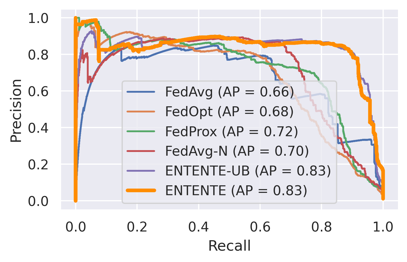
Figure 3. The precision-recall curve under different FL methods on OpTC dataset ($K=3$).

In Figure 3, we draw the precision-recall curve of different FL methods with one client number ($K=3$) due to space limit. The precision of Entente outperforms the other systems at most recall values, and it can reach 0.8 precision at about 0.9 recall.

Table 4. Evaluation on LANL with Euler under different client numbers $K$. Non-FL is listed for ease of comparison.

Client#	3		4		5
Algorithm	AP	AUC	AP	AUC	AP	AUC
Non-FL	0.0089	0.9793	0.0089	0.9793	0.0089	0.9793
FedAVG	0.0010	0.9808	0.0022	0.9841	0.0057	0.9879
FedOpt	0.0060	0.9880	0.0060	0.9908	0.0001	0.8445
FedProx	0.0001	0.8198	0.0019	0.9884	0.0001	0.8164
FedAVG-N	0.0062	0.9797	0.0041	0.9680	0.0053	0.9668
Entente-UB	0.0065	0.9795	0.0082	0.9701	0.0065	0.9733
Entente	0.0087	0.9768	0.0072	0.9700	0.0067	0.9716

Table 5. Evaluation on LANL under different client numbers $K$ on Jbeil. Non-FL is listed for ease of comparison.

	Transductive
Client#	3		4		5
Algorithm	AP	AUC	AP	AUC	AP	AUC
Non-FL	0.9647	0.9751	0.9647	0.9751	0.9647	0.9751
FedAVG	0.6677	0.7298	0.5094	0.5184	0.5964	0.6511
FedOpt	0.8218	0.8581	0.6075	0.6735	0.7258	0.8006
FedProx	0.6729	0.7432	0.7089	0.7787	0.7652	0.8202
FedAVG-N	0.8896	0.9114	0.6192	0.6893	0.6330	0.7016
Entente-UB	0.7747	0.8298	0.9029	0.9147	0.8546	0.8622
Entente	0.8747	0.8880	0.8410	0.8509	0.8105	0.8770
	Inductive
Non-FL	0.9447	0.9621	0.9447	0.9621	0.9447	0.9621
FedAVG	0.6725	0.7389	0.5006	0.5012	0.5877	0.6386
FedOpt	0.8200	0.8612	0.6219	0.6920	0.7516	0.8233
FedProx	0.6828	0.7529	0.7084	0.7796	0.7652	0.8188
FedAVG-N	0.9050	0.9258	0.6385	0.7131	0.6280	0.6977
Entente-UB	0.8212	0.8699	0.9128	0.9265	0.8809	0.8883
Entente	0.8913	0.9049	0.8780	0.8636	0.8056	0.8748

Results on LANL. In Table 4, we show AP and AUC when LANL is tested with Euler. Since Euler uses the redteam events as TP, the class distribution is highly imbalanced, and all systems have low AP. Entente and Entente-UB do not outperform non-FL but are still the ones closest to non-FL in all cases ($K=3,4,5$) in terms of AP. We notice that the trend of AP is somehow opposite to AUC (e.g., AP of Entente is higher than FedAvg when $K=3,5$) and this observation can be attributed to the differences in the training and testing data distribution. In particular, Euler uses negative sampling to “synthesize” malicious edges during training. However, the ground-truth malicious edges during testing have a much smaller volume (only hundreds), which might not be characterized well by the sampled negative edges. Correctly classifying malicious edges is a major goal modeled under AP, but not necessarily so under AUC, when the vast majority of edges are benign. We acknowledge that the AP is still low, and discuss this limitation in Section 6. Yet, we argue that the improvement over the existing systems is more important, and Entente achieves this goal.

Table 5 shows the result when Jbeil is the GNIDS. This time, as non-existent edges are considered as TP (explained in Section 5.1), higher AP is observed. We found Entente still outperforms the other baselines (except $K=3$, lower than FedAVG-N). Though Entente performs worse than Entente-UB, the margin is small. The more balanced class distribution makes non-FL the winner in most cases.

Results on Pivoting. Due to space limit, we present the results in Appendix D. In short, we found Entente achieves the best AP and AUC in the majority of the cases among the FL methods.

5.3. Scalability

Following the scalability requirement described in Section 3.2, we measure the communication overhead and latency caused by Entente.

We first adhere to the default data split setup ($K=2,3,4,5$). Regarding latency, when training LANL and OpTC with Euler, the whole training process takes an average of 116.33 seconds and 706.40 seconds (30 FL iterations till the training converges for LANL and OpTC) and the testing process takes 160.99 seconds and 0.6139 seconds. For Pivoting, the training process takes in average 314.58 seconds (5 FL iterations) and the testing process takes 45.963 seconds.

Compared to the basic FedAVG, Entente introduces extra overhead in generating the global reference graph and updating clients’ weights with WLH and ACS. On LANL, for the first part, only 0.082 seconds is spent, and the second part takes 5.4704, 7.8968, 2.7002, and 0.2395 seconds on the 4 clients separately, when $K=4$. On OpTC, for the first part only 0.0058 seconds is spent and the second one takes 0.5386, 2.2515, 0.8902, 25.6830 when $K=4$. On Pivoting, the first part takes 0.0509 seconds and the second one takes 0.0488, 0.0094, 0.0819 and 0.0349, when $K=4$. The differences between clients are due to their different sizes. The result shows the overhead introduced by Entente is reasonable.

By using FL, Entente also reduces the data transmitted from client to server when training a GNIDS model, saving clients’ bandwidth. Take Euler+LANL as an example. The central server would need to access the 65GB network logs to train GNIDS. With Entente, only model weights $w^{k}_{i}$ are transmitted by a client $k$ in an FL iteration $i$, and only 1.94MB model weights are transmitted in total.

Finally, we attempt to increase $K$ to be more than 5 and test whether Entente can scale up to many clients, and show thete results in Table 6. We evaluate this setting on the LANL dataset because it contains a large number of nodes (17,649). Yet, for large $K$ (e.g., 10 and 20), we found MBM generates empty clusters, so we treat the non-empty clusters as clients (9 and 15 for $K=10$ and $K=20$). We found the training time does increase notably when $K=9$ and $K=15$, but this is because the data loading time is longer (more cross-client edges appear when $K$ increases). Besides, since we simulate all clients on a single machine and they share a GPU, the resource contention also elongate the training time. The training time is expected to reduce when the clients operate in real-world distributed environment. AP and AUC are also recorded, and we found AP are AUC are actually improved for larger $K$.

Table 6. Performance of LANL+Euler under larger client number $K$. “Valid Client#” means the number of valid clients after MBM clustering.

Valid Client#	Training Time	AP	AUC
5	138.51	0.0067	0.9716
9	224.38	0.0077	0.9872
15	497.46	0.0105	0.9912

5.4. Robustness against Poisoning Attacks

In this subsection, we evaluate how Entente performs when FL poisoning attack is conducted by a compromised client. Recently, a few adaptive attacks against GNIDS were developed (Xu et al., 2023; Goyal et al., 2023; Mukherjee et al., 2023). Only Xu et al. (Xu et al., 2023) tested the training-time attacks (the other focused on testing-time attacks). So far, none of the prior works considered the robustness of a GNIDS model trained under FL, and we adapt the attack from Xu et al. (Xu et al., 2023) to our setting, which has been evaluated against Euler on the LANL dataset.

In the original attack of Xu et al. (Xu et al., 2023), covering accesses are added for each malicious edge to avoid exposing the malicious edges when GNIDS is trained. In our setting, the attacker can directly inject the malicious edges to the logs after they are collected by the FL client, under the model poisoning adversary (Bagdasaryan et al., 2020). As such, the covering edges are unnecessary. In addition, the attacker can scale up the model updates by a constant factor $\gamma$ to outweigh the updates from other benign clients (Bagdasaryan et al., 2020).

We present the attack pseudo-code in Algorithm 2. Specifically, on a controlled client $k$, the attacker needs to enumerate all the sub-graphs $[\mathcal{G}_{1}^{k},\dots,\mathcal{G}_{T}^{k}]$ and compare the source and destination nodes to its malicious edges $\mathcal{EM}$ to be used in the testing time. An edge will be added when there is a pair-wise match. We also use a likelihood threshold $p$ to control the number of injected edges.

Data: Number of subgraphs $T$; Malicious edges $\mathcal{EM}$; Likelihood threshold $p$

foreach client $k$ from the malicious clients do

   

   for $t\leftarrow 1$ to T  do

       if random number $<$ p then

         

         for $e\in\mathcal{EM}^{k}$ do

             if $e\not\in\mathcal{E}^{k}_{t}$ and $e.src\in\mathcal{V}^{k}_{t}$ and $e.dst\in\mathcal{V}^{k}_{t}$ then

                $\mathcal{G}^{k}_{t}.add(e)$;

               

            

         

      

   Send $\gamma$ $\times$ ClientUpdate($k,w_{i}$) to central server in each FL iteration

Algorithm 2 The proposed poisoning attack. ClientUpdate is the same as Algorithm 4. Each client’s graph $\mathcal{G}^{k}=(\mathcal{V}^{k},\mathcal{E}^{k})$

Since the poisoning attack conducted by Xu et al (Xu et al., 2023) is on Euler+LANL, we focus on attacking the Euler GNIDS. We test both LANL and OpTC datasets to evaluate the generality of the attack. In Table 7, we show the attack result when Euler is trained on LANL under Entente. We select client 4 as the malicious client, which observes 495 malicious edges (out of 517 total malicious edges). Among these edges, 492 are cross-client edges, so the attacker has the motivation to poison the global model to hide their attack from the other clients. We define “success rate” (SR) as the ratio of malicious edges that evade detection, which is similar to Xu et al. (Xu et al., 2023). We also count the number of injected edges per malicious edge (EPM). EPM could be larger than 1 when multiple snapshots are poisoned. $\gamma$ is set to values between 5 and 100 and $p$ is set to values between 25% to 100%. The row with “-” in $\gamma$ and $p$ in Table 7 shows result without attack. The attack is more powerful with larger $\gamma$ and $p$. The result shows Entente can bound SR to a low number (9.30%). When disabling the norm bounding defense (Entente-UB), training GNIDS model observes higher SR, but more importantly, “NaN” (not a number) error occurs with larger $p$ and $\gamma$. In this case, the gradient updates accumulate substantial changes, leading to sudden large adjustments of the global model weights and gradient explosion. Training the GNIDS model will fail, which maps to the untargeted attack against FL (Fang et al., 2020).

Table 7. Attack on LANL ($K=4$). Client 4 is malicious. The upper (“E”) and lower parts (“EUB”) of the table shows the result of Entente and Entente-UB.

	$p$	$\gamma$	AP	AUC	SR	EPM
E	-	-	0.0072	0.9700	-
	25%	5	0.0054	0.9696	9.30%	22
	50%	5	0.0056	0.9697	9.30%	40
	50%	25	0.0056	0.9697	9.30%	40
	75%	25	0.0060	0.9699	9.30%	62
	100%	100	0.0055	0.9696	9.30%	80
EUB	25%	5	0.0074	0.9734	11.4%	22
	50%	25	0.0018	0.9623	40.59%	22
	100%	100	NaN	NaN	-	80

Regarding OpTC, we choose $K=3$ and use client 3 as a malicious client. Similar as the result on LANL, Entente is robust even under very large $p$ and $\gamma$, as shown in Table 8. Without the norm bounding defense, much higher SR is observed or the training process cannot finish.

Table 8. Attack on OpTC ($K=3$). Client 3 is malicious. The upper (“E”) and lower (“EUB”) parts of the table shows the result of Entente and Entente-UB.

	$p$	$\gamma$	AP	AUC	SR	EPM
E	-	-	0.8329	0.9976	-
	10%	2	0.8370	0.9972	17.65%	148
	25%	5	0.8348	0.9976	14.61%	374
	50%	10	0.8569	0.9978	13.38%	764
	100%	100	0.8491	0.9975	14.20%	1513
EUB	10%	2	0.7294	0.9930	28.24%	148
	50%	5	NaN	NaN	-	764
	100%	25	NaN	NaN	-	1513

5.5. Ablation Study

Impact of ACS. We introduce ACS to dynamically adjust the clients’ weights of each iteration. Here we measure its contributions, by comparing the AP and AUC of Entente with and without it. We found that ACS increases AP and AUC in nearly every combination of GNIDS, dataset, and $K$. Taking AP as an example, the increases averaged among $K$ are 0.0776 for OpTC+Euler, 0.0024 for LANL+Euler, 0.1463 (Transductive) and 0.1668 (Inductive) for LANL+Jbeil, and 0.0653 (Transductive) and 0.0753 (Inductive) for Pivoting+Jbeil.

In Figure 4, we illustrate the changes of client weight along FL iterations, and we show the result of LANL+Euler when $K=4$ due to space limit. It turns out ACS is able to notably adjust the client weights, e.g., Client 3 and 4 after Epoch 15, which addresses the issue of gradient instability when updating the global model.

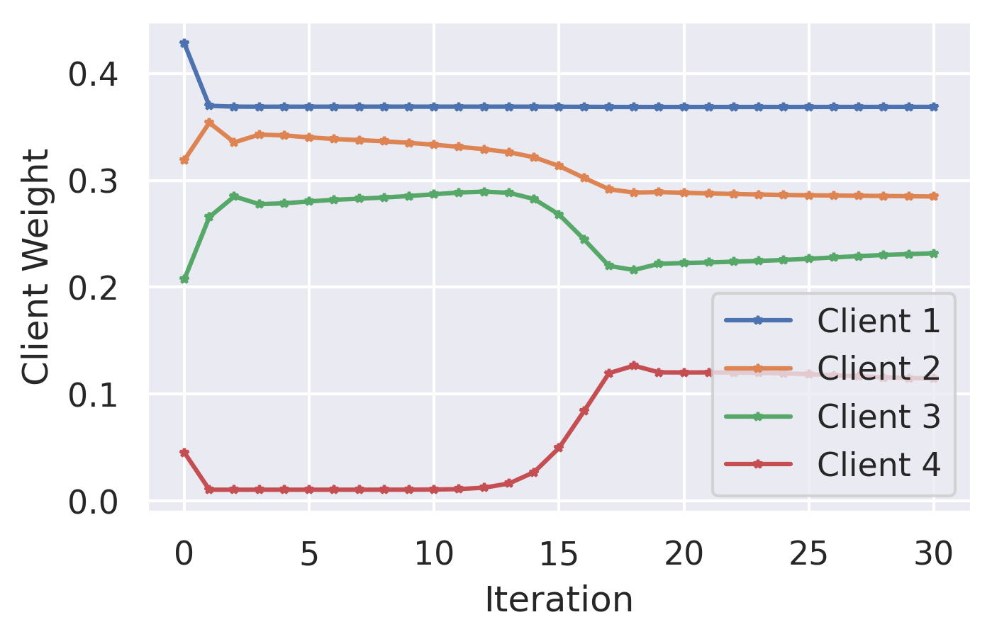
Figure 4. The client weight updating on LANL ($K=4$).

Impact of graph augmentation. We propose to augment each client’s subgraph with 1-hop cross-client edges as described in Section 4.1. Here we evaluate the contribution of this technique. We rerun the experiments for OpTC ($K=3$) and LANL ($K=4$) when Euler is the GNIDS without adding the cross-client edges. The result is shown in Table 9. It shows prominent improvement with graph augmentation: over 0.82 and 0.56 increase in AP and AUC on OpTC is achieved, and 0.0061 and 0.007 increase in AP and AUC on LANL is achieved.

Table 9. Analysis of graph augmentation. “1-hop” is the default setting. “None” means the cross-client edges are not added. Euler is the GNIDS.

Dataset	Augmentation	AP	AUC
OpTC ($K=3$)	None	0.0101	0.4380
	1-hop	0.8329	0.9976
LANL ($K=4$)	None	0.0011	0.9623
	1-hop	0.0072	0.9700

Other ablation study. In Appendix E, we provide more ablation study results, including the impact of $K$ and $m$, comparison between local and global models, and visualization of MBM clustering.

6. Discussion

Differential privacy for Entente. To protect the privacy of FL clients, differential privacy (DP) has been leveraged to add noises to the model updates, which could hide the existence of a single instance for cross-silo FL (Xie et al., 2023). Interestingly, poisoning attacks can also be deterred by DP, as discovered by previous works  (Sun et al., 2019; Xie et al., 2023; Geyer et al., 2017; Zhang et al., 2022b). Here we provide a cursory analysis regarding the combination of DP and Entente. In Appendix F, we describe the test results, which however suggest maintaining reasonable model utility while curbing the poisoning attack is still challenging.

Limitations and future works. First, we admit that the results of Entente on LANL are far from ideal when the redteam events are TP. A few reasons have been given in prior works (King and Huang, 2023; Xu et al., 2024), including: 1) the labeled malicious events are too coarse-grained; 2) the malicious activities after the redteam’s ground-truth events are not tracked; 3) potentially malicious events on included in the “attack-free” training period. Second, due to the lack of ground truth of the locations of each device in the LANL or OpTC dataset, we choose to run the clustering method MBM (Larroche, 2022a) to generate FL clients’ data. The location information is usually not provided from a log dataset and the IP is also anonymized. Clustering is our best effort. Similar approaches have been followed by other FGL works like  (Yao et al., 2022; Zhang et al., 2021a; Xie et al., 2021). Third, we did not simulate Entente and other baseline FL methods in a fully distributed environment, i.e., different clients on different machines. Hence, the actual overhead, especially network communication, should be higher. However, the extra overhead caused by Entente over the basic FedAVG method is introduced during bootstrap and ACS, and Section 5.2 shows it is reasonable. Finally, we did not simulate different FL poisoning attacks (surveyed in Section 7) besides Xu et al. (Xu et al., 2023), due to the gap between the attack methods and the concrete GNIDS setting. We leave the exploration of new attacks as a future work.

7. Related Work

Host-based Intrusion Detection (HIDS). This work focuses on developing privacy-preserving GNIDS, which consumes network logs. Graph learning has also been applied on host logs. We refer interested readers to a survey by Inam et al.  (Inam et al., 2023) for details. Below we provide a brief overview. The main approach to detect intrusions under HIDS is through provenance tracking (King and Chen, 2005; Jiang et al., 2006), which performs variations of breadth-first search (e.g., under temporal constraints like happens-before relation (Shu et al., 2018)) to find other attack-related nodes given Indicators of Compromise (IoCs). Yet, provenance tracking often leads to a large number of candidate nodes to be investigated (Xu et al., 2016), and many HIDS add heuristics to reduce the investigation scope (Hassan et al., 2019; Liu et al., 2018; Milajerdi et al., 2019; Hossain et al., 2020). Another way to reduce the false positives is to simplify the graphs, e.g., through event abstraction (Hassan et al., 2020; Yu et al., 2021) and graph summation (Xu et al., 2022).

Recently, like GNIDS, GNN has also been tested for HIDS and various embedding techniques have been developed/used, including masked representation learning (Jia et al., 2023), TGN (Cheng et al., 2024), Graph2Vec  (Yang et al., 2023b), embedding recycling (Rehman et al., 2024), root cause embedding (Goyal et al., 2024), etc. It is likely that FL could benefit these HIDS, but different operational model and/or learning method is needed. For instance, cross-device FL instead of cross-silo FL is a more suitable FL setup.

FL for security. Before our work, FL has been applied in various security-related settings, like risk modeling on mobile devices (Fereidooni et al., 2022), malicious URL detection (Khramtsova et al., 2020; Ongun et al., 2022), detecting abnormal IoT devices (Nguyen et al., 2019), malware detection (Rey et al., 2022), browser fingerprinting detection (Annamalai et al., 2024), etc. Though FL has also been used to train an anomaly detector on system logs (De La Torre Parra et al., 2022; Naseri et al., 2022), these work treat logs as tabular data while we model logs as graphs.

Security and privacy for FL. Here, we present a more detailed overview of security and privacy issues in FL. Regarding security, poisoning (or backdoor) attacks are considered as the major threat (Mothukuri et al., 2021), and the previous attacks can be divided into data poisoning (Nguyen et al., 2020; Shen et al., 2016; Xie et al., 2019) that manipulates the clients’ training data and model poisoning (Bagdasaryan et al., 2020; Wang et al., 2020; Li et al., 2023b; Krauß et al., 2024) that manipulates the training process or models themselves. In either case, poisoning will result in deviation of model updates, and the majority of defenses aim to detect and mitigate abnormal deviation (Rieger et al., 2022; Nguyen et al., 2022; Kumari et al., 2023; Fereidooni et al., 2024; Sun et al., 2019; Rieger et al., 2024; Kabir et al., 2024). Entente integrates norm bounding (Sun et al., 2019) into the training procedure and the empirical and theoretical results show its effectiveness.

Though FL is supposed to protect the privacy of clients’ data, attacks like membership inference attacks (MIA) can still leak private information (Nasr et al., 2019). As a countermeasure, differential privacy (DP) has been applied to FL, and the noises can be added to each training step with DP-SGD (Sun et al., 2021; Truex et al., 2020), to the trained local model (Agarwal et al., 2021; Kairouz et al., 2021) and to the central server (Geyer et al., 2017; McMahan et al., 2018). Recently, Yang et al. studied the accuracy degradation caused by FL+DP, and exploited client heterogeneity to improve the FL model’s accuracy (Yang et al., 2023a). We attempted to integrate DP into Entente but the accuracy drop is prominent. We also believe the privacy threat and the privacy notions need to be clearly defined under the GNIDS setting, in order to enable more effective defense.

8. Conclusion

In this paper, we propose Entente, a new Graph-based Network Intrusion Detection Systems (GNIDS) backed by Federated Learning (FL), to address concerns in data sharing. We carefully tailor the design of Entente to the unique settings of the security datasets (e.g., highly imbalanced classes and non-IID client data) and variations of GNIDS tasks/architectures. With new techniques like weight initialization and adaptive contribution scaling, we are able to achieve the desired design goals (effectiveness, scalability and robustness) altogether. The evaluation of three large-scale log datasets, namely OpTC, LANL and Pivoting, shows that Entente outperforms the other baseline systems, even including the model trained on the whole dataset in some cases. We also conduct adaptive attacks against Entente with FL poisoning, and show Entente can bound the attack success rate and ensure the training procedure can finish as desired. With Entente, we hope to encourage more research to address the data sharing issues in building GNIDS, which is under-studied, and develop better attack and defense benchmarks to evaluate the robustness of federated graph learning (FGL) systems.

Appendix A Algorithm of BA Model

In Algorithm 3, we describe BA model with pseudo-code.

Data: $n$ (number of nodes), $m$ (number of edges to attach from a new node to existing nodes)

Result: $G$ (generated graph)

$G\leftarrow\text{InitializeGraph}(m)$;

for $i=m+1$ to $n$ do

    $\text{AddNode}(G,i)$;

    $k_{j}\leftarrow\text{Degree}(G)$;

    $K\leftarrow\sum_{j\in G}k_{j}$;

    $L\leftarrow\text{EmptyList}()$;

    foreach $j\in G$ do

       $L.\text{Add}(j,k_{j}/K)$;

      

   $S\leftarrow\text{RandomSelect}(L,m)$;

    foreach $v\in S$ do

       $\text{AddEdge}(G,i,v)$;

      

   

return $G$

Algorithm 3 Barabási–Albert (BA) Model

Appendix B Workflow of Entente

In Algorithm 4, we summarize the workflow of Entente. Specifically, $w_{i}$ contains the model parameters for graph encoder, temporal encoder and decoder, which are denoted by $\text{ENC}(\cdot)$, $\text{TEMP}(\cdot)$ and $\text{DEC}(\cdot)$. For decoder, only the trainable implementations go through FL. $\text{JS}(\cdot)$ is Jaccard similarity. $\nabla\mathcal{L}$ computes gradients on training loss, and the same loss function of the GNIDS is used.

Data: $E$ is the number of local epochs; $\eta$ is the learning rate; Number of maximum FL iterations $R$; Number of subgraphs $T$; $c_{1}$ and $c_{2}$ are two constants.

Result: Global model parameters $w_{i+1}$

Server executes:

Initialize $w_{1}$;

$\mathcal{G}^{ref}$ $\leftarrow$ BA_Model($n$, $m$);

foreach client $k$ from all clients do

    $S_{Jac}^{k}$ $\leftarrow$ ClientInitialWeight($k,\mathcal{G}^{ref}$);

   

for $i=1$ to $R$ do

    foreach client $k$ from all clients do

       $w^{k}_{i}$ $\leftarrow$ ClientUpdate($k,w_{i}$);

      

   $S^{K}_{i},D^{K}_{i}=$ ACS($w_{i},w^{k}_{i}$);

    $w_{i+1}[\text{ENC}]$ $\leftarrow$ $w_{i}[\text{ENC}]$ + $\Sigma^{K}_{k=1}(c_{1}\times S^{k}_{Jac}+c_{2}\times S^{k}_{i}\times D^{k}_{i})\times\mathsf{NB}(\Delta w^{k}_{i+1}[\text{ENC}])$ ;

    $w_{i+1}[\text{TEMP}]$ $\leftarrow$ $w_{i}[\text{TEMP}]+\Sigma^{K}_{k=1}(c_{1}\times S^{k}_{Jac}+c_{2}\times S^{k}_{i}\times D^{k}_{i})\times\mathsf{NB}(\Delta w^{k}_{i+1}[\text{TEMP}]$ ;

    if  DEC is trainable then

       $w_{i+1}[\text{DEC}]$ $\leftarrow$ $w_{i}[\text{DEC}]+\Sigma^{K}_{k=1}(c_{1}\times S^{k}_{Jac}+c_{2}\times S^{k}_{i}\times D^{k}_{i})\times\mathsf{NB}(\Delta w^{k}_{i+1}[\text{DEC}]$ ;

      

   

   if early_stopping($w_{1},\dots,w_{i+1}$) then

       break;

      

   

return $w_{i+1}$

Function ClientInitialWeight($k,\mathcal{G}^{ref}$):

    Generate local graph $\mathcal{G}^{k}$;

    Add cross-client edges to $\mathcal{G}^{k}$;

    $[\mathcal{G}_{1}^{k},\dots,\mathcal{G}_{T}^{k}]$ $\leftarrow$ separate($\mathcal{G}^{k}$);

    return JS(WLH($\mathcal{G}^{k}$), WLH($\mathcal{G}^{ref}$)) to server;

   

Function ACS($w_{i},w^{k}_{i}$):

    Compute $S^{K}_{i}$ and $D^{K}_{i}$ ;

    return $S^{K}_{i},D^{K}_{i}$ to server;

   

Function ClientUpdate($k,w$):

    for each local epoch $i$ from 1 to E do

       $w\leftarrow w-\eta\nabla\mathcal{L}(w;[\mathcal{G}_{1}^{k},\dots,\mathcal{G}_{T}^{k}])$;

      

   return $w$ to server;

   

Algorithm 4 Global model training under Entente.

Table 10. Evaluation on different datasets with client number $K=2$.

Euler on OpTC Client# 2 Algorithm AP AUC Non-FL 0.6996 0.9876 FedAVG 0.3369 0.9578 FedOpt 0.6662 0.9837 FedProx 0.6429 0.9807 FedAVG-N 0.7041 0.9913 Entente-UB 0.7714 0.9950 Entente 0.7460 0.9941

Euler on LANL Client# 2 Algorithm AP AUC Non-FL 0.0089 0.9793 FedAVG 0.0071 0.9808 FedOpt 0.0065 0.9787 FedProx 0.0072 0.9790 FedAVG-N 0.0051 0.9685 Entente-UB 0.0070 0.9707 Entente 0.0077 0.9892

Jbeil on LANL (Transductive) Client# 2 Algorithm AP AUC Non-FL 0.9647 0.9751 FedAVG 0.8854 0.9185 FedOpt 0.5967 0.6464 FedProx 0.6100 0.6771 FedAVG-N 0.7137 0.7746 Entente-UB 0.9540 0.9647 Entente 0.9443 0.9625

Jbeil on LANL (Inductive) Client# 2 Algorithm AP AUC Non-FL 0.9447 0.9621 FedAVG 0.8730 0.9134 FedOpt 0.5879 0.6350 FedProx 0.6280 0.6994 FedAVG-N 0.6733 0.7413 Entente-UB 0.9554 0.9655 Entente 0.9358 0.9588

Appendix C Datasets and pre-processing

The OpTC dataset (Five Directions, 2020) contains the telemetry data collected under the DARPA TC program (DARPA, 2014), during which APT attacks were simulated on different OSes. The host-level activities between subjects like processes and objects like files and sockets were logged. Like Euler (King and Huang, 2023), we use the “START” events related to the “FLOW” objects (i.e., network flows). The nodes are hosts distinguished by IP addresses and the flows between hosts are merged into edges. The statistics after this step are shown in Table 2. We split the data into 6 minutes (360s) window. We use the first 5 days’ snapshots (no redteam events exist) for training and the remaining 3 days’ snapshots for testing. OpTC is only tested by Euler and we report its result accordingly.

The LANL dataset (Kent, 2015) contains anonymized event data from four sources within Los Alamos National Laboratory’s internal computer network. We use the authentication logs from individual computers and domain controller servers following (King and Huang, 2023; Khoury et al., 2024). Simulated redteam attacks are conducted from the compromised machines. As shown in Table 2, the malicious events consist of a fairly small portion among all events, posing a great challenge to GNIDS. Regarding data pre-processing, like  (King and Huang, 2023; Khoury et al., 2024), we only keep the events with the keyword “NTLM” (Microsoft, 2021), as other events are unrelated to authentications. For Euler, the logs are split by a 30-minute (1,800s) window into snapshots. We use “source computer” and “destination computer” as nodes and all events sharing the same pairs of nodes are merged into an edge. The first 42 hours are used to train the Euler GNIDS. On average, each snapshot has 7,957 edges and we use 5% edges for validation. After 42 hours, redteam events appear and the following snapshots are used for testing. For Jbeil, we follow their pre-processing procedures to use the events that happened during the first 14 days, including 12,049,423 events. Different from Euler, Jbeil did not use the LANL’s redteam events as malicious samples. Instead, it injects non-existent edges (i.e., negative sampling) and conducts link prediction (i.e., predicting an edge’s existence in testing). We use 70% events for training, 15% for validation and the remaining 15% for testing. For the transductive learning mode, the training and testing sets share the same set of nodes. For the inductive learning mode, 30% of the nodes are hidden during the training but unmasked during testing, following Jbeil’s setting.

The Pivoting dataset (Apruzzese et al., 2017) comprises network flow data, collected over a full working day under a large organizational setting, exclusively representing internal-to-internal communications among hosts. The simulated pivoting activities for lateral movement are considered malicious. It is only tested by Jbeil and we follow its setting and used the first 1,000,000 events, which correspond to 698 nodes. Again, the data is split into 70% for training, 15% for validation, and the remaining 15% for testing. Link prediction is conducted and we test both transductive and inductive learning modes.

Appendix D More Results on LANL, OpTC and Pivoting Dataset

Table 10 shows the effectiveness results when the client number $K=2$ under the same setting of Section 5.2. Again, Entente or Entente-UB achieve the best results among the FL methods.

Table 11 shows the results on the Pivoting dataset when Jbeil is the GNIDS. We observe that Entente achieves the best AUC in most cases ($K=2,4$ for transductive mode and $K=3,4$ for inductive mode). FedOpt outperforms Entente when $K=2$ and Entente-UB outperforms when $K=3$ for transductive but the differences are small (less than 5%). Though non-FL achieves the best AP and AUC in nearly all cases, the margins over Entente are also small (less than 0.07 AP and 0.04 AUC).

Table 11. Evaluation on Pivoting with Jbeil. Non-FL is listed for ease of comparison.

	Transductive
Client#	2		3		4
Algorithm	AP	AUC	AP	AUC	AP	AUC
Non-FL	0.9626	0.9705	0.9626	0.9705	0.9626	0.9705
FedAVG	0.8207	0.8870	0.6881	0.7570	0.8119	0.8726
FedOpt	0.9581	0.9702	0.8114	0.8737	0.9028	0.9397
FedProx	0.8101	0.8734	0.8072	0.8671	0.5862	0.6256
FedAVG-N	0.7414	0.8064	0.9338	0.9621	0.9579	0.9750
Entente-UB	0.9355	0.9600	0.8972	0.9391	0.9478	0.9624
Entente	0.9554	0.9721	0.9098	0.9468	0.9640	0.9777
	Inductive
Non-FL	0.9592	0.9687	0.9592	0.9687	0.9592	0.9687
FedAVG	0.8359	0.8946	0.7105	0.7806	0.8080	0.8699
FedOpt	0.9621	0.9744	0.8570	0.9087	0.9165	0.9494
FedProx	0.8058	0.8717	0.8153	0.8740	0.5808	0.6199
FedAVG-N	0.7282	0.7881	0.8762	0.9241	0.9268	0.9584
Entente-UB	0.9146	0.9486	0.8753	0.9258	0.9096	0.9397
Entente	0.9288	0.9585	0.8905	0.9358	0.9319	0.9609

Appendix E More Ablation Study

Client number ($K$). Here, we take a closer look at the effectiveness results under different $K$. We found Entente, FedOpt and FedProx are less sensitive to different $K$ values, suggesting their robustness under different client settings. The changes on FedAvg can be drastic, e.g., AP dropping from 0.7519 ($K=5)$ to 0.3369 ($K=2$) for OpTC+Euler, and from 0.8854 ($K=2$) to 0.5094 ($K=4$) for LANL+Jbeil+Transductive. Though FedAVG-N sometimes can outperform Entente, it is not as stable as Entente, e.g., AP dropping from 0.9338 to 0.7414 for Pivoting+Jbeil+Transductive.

Table 12. Standard deviation of node and event numbers among different clients under different $K$. “Non-FL” shows the numbers when GNIDS is trained on the whole dataset.

		Non-FL	2	3	4	5
Nodes	OpTC	814	475	408	359	324
	LANL	17,649	10,858	5,626	5,139	4,721
	Pivoting	1,015	112	139	107	-
Events	OpTC	92,095,501	864,643	759,024	673,283	609,197
	LANL	1,051,431,208	33,407	5,470,379	6,438,577	6,814,546
	Pivoting	74,551,643	36,904,845	34,684,014	31,569,225	-

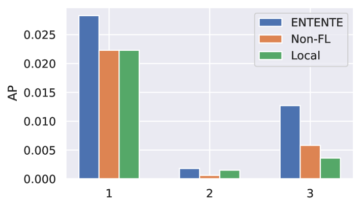
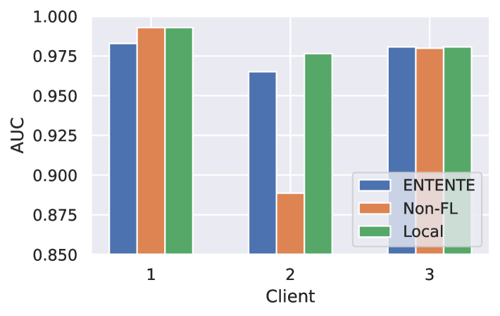
Figure 5. The AP and AUC of Entente’s global model, non-FL model and local model on each local dataset. LANL+Euler is tested and $K=3$.

We also examine the client clusters, by measuring the standard deviation of the node numbers and event numbers across clients. The result is shown in Table 12. For LANL, the standard deviation of node numbers is the highest when $K=2$, which is over 40% of the total node numbers, and it is significantly reduced for when $K>2$. Entente turns out to achieve stable AP and AUC across different $K$, especially when Euler is the GNIDS, suggesting Entente can self-adjust to different client distributions. For OpTC, we also observe high standard deviation of node numbers. For Pioviting, though the standard deviation of node numbers are relatively small, we observe very high standard deviation of event numbers. Overall, the data distribution reflects the non-iid challenge discussed in Section 3.2.

The number of initial edges for a new node ($m$). We use the BA model to generate the reference graph. We set $m$ as 5 by default. Decreasing and increasing $m$ could make the reference graph denser or sparser, which could impact the weights computed for each client. To assess its impact, we set $m=2,4,5,10,100$ and compute AUC and AP on LANL with Euler GNIDS ($K=3$). We find the result does not change, suggesting Entente is not sensitive to the value of $m$.

Comparison between local and global models. Each client obtains a global model from the central server after FL. On the other hand, the client can just train a local model on its own data and ignore the global model, when it considers the global model does not bring benefit. As such, we compare Entente’s global model with the trained local model on each client. For a fair comparison, the cross-client edges have been added to each client’s graph when training the local model. We also test how non-FL performs on each client’s data separately.

In Figure 5, we show the comparison of Entente’s global model, Non-FL, and local model on 3 clients of LANL,. For AP, Entente outperforms the other methods on all clients (0.0283, 0.0018, 0.0127). Client 1 and client 3 have a higher AP margin because many malicious edges (47.41% and 40.79%) reside in both clients. The result shows that for a client, aggregating information from other clients is beneficial.

Cluster generation. We leverage MBM to cluster machines of a log dataset and form clients. Here we provide a visualized example of the clustering result on LANL in Figure 6 with the MBM code (Larroche, 2022b). We set the the number of machine clusters, which equals to the client number $K$, to 4. MBM is able to generate machine clusters of variable sizes (ranging from 129 to 15,941) and preserve the prominent interactions between user clusters and machine clusters (e.g., host cluster 1 connects to user cluster 0, 1 and 2).

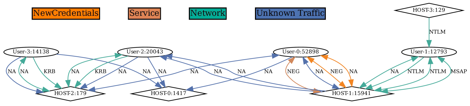
Figure 6. Visualization of the clustering done by MBM for LANL ($K=4$). We use ellipses to show user clusters and the number in the ellipses are the user number. For hosts (or machines), we use diamonds and provide host numbers. The legend in different colors summarizes the major traffic type between user clusters and machine clusters: New Credentials, Service, Network and Unknown Traffic. Each edge represents one protocol type. “KRB” means Kerberos; “NEG” means Negotiate; “MSAP” means Microsoft Authentication Package. “’NA” means unknown protocols.

Table 13. Defenses against strongest poisoning ($p=100\%$, $\gamma=100$) on LANL ($K=4$). Client 4 is malicious. “-” in “Defense” means no defense is enabled.

Type	Defense	AP	AUC	SR
No attack	-	0.0072	0.9700	-
	Weak DP	0.0006	0.9523	-
	CDP	0.0054	0.9636	-
With attack	Weak DP	0.0011	0.9521	2.77%
	CDP	0.0054	0.9637	9.10%

Table 14. Defenses against strongest poisoning ($p=100\%$, $\gamma=100$) on OpTC ($K=3$). Client 3 is malicious.

Type	Defense	AP	AUC	SR
No attack	-	0.8329	0.9976	-
	Weak DP	0.7475	0.9666	-
	CDP	0.2404	0.8694	-
With attack	Weak DP	0.7401	0.9666	16.25%
	CDP	0.2403	0.8695	38.66%

Appendix F Differential Privacy for Entente

Specifically, Equation 10 can be adjusted to integrate DP as written below:

(12) $$w_{i+1}=w_{i}+\frac{1}{K}\sum^{K}_{k=1}r^{k}_{k}\times\mathsf{NB}(\Delta w^{k}_{i+1})+\mathcal{N}(0,M_{\mathsf{qs}}^{2}\sigma^{2})$$

We are able to support weak DP (Sun et al., 2019) and CDP (Geyer et al., 2017; Zhang et al., 2022b) defenses with Equation 12. Their difference is the value of $M_{\mathsf{qs}}$. Weak DP extends norm bounding by adding a Gaussian noise under small variance $\sigma$ to each model update, and the value of $M_{\mathsf{qs}}$ is relatively smaller than expected as the standard DP. CDP requires the noise level to be proportional to the sensitivity.

We set $\omega$, $M$, $\epsilon$ and $\delta$ to 5.0, 5.0, 1.0, 0.1 and $\sigma$ as 1.0 for Weak DP and 0.2 for CDP after empirical analysis. The results of LANL and OpTC from Table 13 and Table 14 show that though both defenses are effective against our poisoning attack, with Weak DP more effective in dropping SR, they also significantly drop GNIDS’s AP even when no attack is launched (e.g., 0.0072 dropped to 0.0006 for LANL+Weak DP and 0.8329 dropped to 0.2404 for OpTC+CDP).

Appendix G Theoretical Analysis

G.1. Proof of Theorem 1

Proof.

With Equation 9, we have,

$$|w_{i+1}| =|\sum^{K}_{k=1}(c_{1}\times S_{\mathsf{Jac}}^{k}+c_{2}\times S^{k}_{i}\times D^{k}_{i})\times w^{k}_{i}|$$

$$\leq\sum^{K}_{k=1}|(c_{1}\times S_{\mathsf{Jac}}^{k}+c_{2}\times S^{k}_{i}\times D^{k}_{i})\times w^{k}_{i}|$$

$$\leq\sum^{K}_{k=1}|(c_{1}\times S_{\mathsf{Jac}}^{k}+c_{2}\times S^{k}_{i}\times D^{k}_{i})|\times|w^{k}_{i}|$$

Given Equation 8, we know that $D^{k}_{i}=\omega$ if $\sqrt{\sum(w_{i}^{k}-w_{i-1})^{2}}\geq\omega$; otherwise $D^{k}_{i}=\sqrt{\sum(w_{i}^{k}-w_{i-1})^{2}}$ if $\sqrt{\sum(w_{i}^{k}-w_{i-1})^{2}}<\omega$. Thus, we bound $D_{1}^{k}\leq\omega$ for any $\omega>0$. In practice, $\omega=1$ can be done by normalization.

Jaccard similarity $S_{\mathsf{Jac}}^{k}$ and Cosine similarity $S^{k}_{i}$ satisfy $0\leq S_{\mathsf{Jac}}^{k},S^{k}_{i}\leq 1$. For a preset positive integer $K$, we can simplify the inequality above and get,

$$|w_{i+1}| \leq\frac{1}{K}\sum^{K}_{k=1}|(c_{1}\times 1+c_{2}\times 1\times\omega)|\times|w^{k}_{i}|$$

$$\leq\sum^{K}_{k=1}\frac{|(c_{1}+c_{2}\omega)|\times|w^{k}_{i}|}{K}$$

$$=|(c_{1}+c_{2}\omega)|\frac{\sum^{K}_{k=1}|w^{k}_{i}|}{K}$$

$$\Rightarrow|\frac{w_{i+1}}{(1/K)\sum_{k}w^{k}_{i}}| \leq c_{1}+c_{2}\omega$$

∎

G.2. Proof of Theorem 2

In Entente, at each round $i\in[R]$, we solve an optimization problem in the following form,

(13) $$\min_{x\in\mathbb{R}^{d}}f(w_{i+1})=\frac{1}{K}\sum_{k=1}^{K}F_{k}(w_{i})$$

where $k\in[K]$ be a client index for $K$ clients. For the $k$-th client, we define its loss function by,

(14) $$F_{k}(w)=\mathbb{E}_{z\sim\mathrm{data}_{k}}[f_{k}(w,z)]$$

where $\mathrm{data}_{k}$ is the client’s data distribution. For different clients, $\mathrm{data}_{k}$ can be heterogeneous. Recall in FedAVG, $F_{k}(w_{i})=w_{i}$.

At each round $i$, we assume all $K$ clients participate in and contribute to updating the global model. Following the notations used in Algorithm 4, $E$ is the number of local epochs; $\eta$ is the learning rate used in local models; $R$ is the number of maximum FL iterations; $c_{1}$ and $c_{2}$ are the predetermined hyperparameters to adjust contributors; $d$ is the dimension of $w$.

Before analyzing the convergence of Entente, we first introduce the prior knowledge (Reddi et al., 2021; Zhang et al., 2022b) and common settings (Zaheer et al., 2018; Reddi et al., 2016; Kingma and Ba, 2015) that we rely on. We adopt the standard assumption in Lemma 1 (Zaheer et al., 2018; Reddi et al., 2016; Kingma and Ba, 2015) for nonconvex optimization as $F_{k}$ may be nonconvex. $\nabla F_{k}(x)$ is defined as the computed gradients of each client. As for federated optimization, we consider the setting of bounded variance and gradients (Li et al., 2020b; Reddi et al., 2021; Zhang et al., 2022b) as in Lemmas 2,3 and Lemmas 4, which are widely adopted for heterogeneity analysis.

Lemma 0 (Lipschitz Gradient).

The function $F_{k}$ is $L$-smooth for any $k\in[K]$ such that,

(15) $$\|\nabla F_{k}(x)-\nabla F_{k}(y)\|\leq L\|x-y\|,\quad\forall\ x,y\in\mathbb{R}^{d}$$

Lemma 0 (Bounded Local Variance).

The function $F_{k}$ has $\sigma_{\mathsf{local}}$-bounded local variance such that,

(16) $$\mathbb{E}[\|\nabla[f_{k}(w,z)]_{j}-[\nabla F_{k}(w)]_{j}\|]=\sigma_{\mathsf{local},j}^{2}$$

for all $w\in\mathbb{R}^{d},j\in[d]$, and $k\in[K]$.

Lemma 0 (Bounded Global Variance).

The function $F_{k}$ has $\sigma_{\mathsf{global}}$-bounded global variance such that,

(17) $$\frac{1}{K}\sum_{k=1}^{K}\|\nabla[F_{k}(w)]_{j}-[\nabla f(w)]_{j}\|\leq\sigma_{\mathsf{global},j}^{2}$$

for all $w\in\mathbb{R}^{d}$ and $j\in[d]$.

Lemma 0 (Bounded Gradients).

The gradients of function $f_{k}(w,z)$ is $G$-bounded such that,

(18) $$|[\nabla f_{k}(w,z)]_{j}\leq G|,\quad\forall\ j\in[d]$$

for any $k\in[K],w\in\mathbb{R}^{d}$ and $z\sim\mathrm{data}_{k}$.

Proof.

To analyze the convergence of Entente, we need to express the global model difference $w_{i+1}-w_{i}$ between any consecutive rounds $i,i+1$. By Equation 10, the global model difference can be calculated by,

$$w_{i+1}-w_{i}=\frac{1}{K}\sum^{K}_{k=1}(c_{1}\times S_{\mathsf{Jac}}^{k}+c_{2}\times S^{k}_{i}\times D^{k}_{i})\times\mathsf{NB}(\Delta w^{k}_{i+1})$$

At the $i$-th iteration, the learning rate of updating $w_{i}+1$ is $c_{1}\times S_{\mathsf{Jac}}+c_{2}\times S^{k}_{i}\times D^{k}_{i}$ at each client. Using Lipschitz smoothness, we get,

$$\mathbb{E}[f(w_{i+1})]\leq f(w_{t})$$

$$+\left\langle\nabla f(w_{t}),\mathbb{E}[\frac{1}{K}\sum^{K}_{k=1}(c_{1}\times S_{\mathsf{Jac}}^{k}+c_{2}\times S^{k}_{i}\times D^{k}_{i})\times\mathsf{NB}(\Delta w^{k}_{i+1})]\right\rangle$$

$$+\frac{L}{2}\mathbb{E}\left[\|\frac{1}{K}\sum^{K}_{k=1}(c_{1}\times S_{\mathsf{Jac}}^{k}+c_{2}\times S^{k}_{i}\times D^{k}_{i})\times\mathsf{NB}(\Delta w^{k}_{i+1})\|\right]$$

In Theorem 1, we know $r^{k}_{i}=c_{1}\times S_{\mathsf{Jac}}^{k}+c_{2}\times S^{k}_{i}\times D^{k}_{i}\leq c_{1}+c_{2}\omega$ for any positive $c_{1},c_{2}$. Norm bounding is defined by $\mathsf{NB}(\Delta w^{k}_{i+1})=\frac{\Delta w^{k}_{i+1}}{\max(1,\lVert\Delta w^{k}_{i+1}\rVert_{2}/M)}$ (Sun et al., 2019). The bounding ensures that if $\|\Delta w^{k}_{i+1}\|_{2}\leq M$, $w^{k}_{i+1}$ is preserved for further computation; otherwise, if $\|\Delta w^{k}_{i+1}\|_{2}>M$, the norm of $\Delta w^{k}_{i+1}$ is equal to $M$. For simplifying notations, we define,

$$\alpha^{k}_{i}=\frac{(c_{1}\times S_{\mathsf{Jac}}^{k}+c_{2}\times S^{k}_{i}\times D^{k}_{i})M}{\max(M,\eta\|\sum_{e=1}^{E}g^{k,e}_{i}\|)}$$

where $g^{k,e}_{i}$ is the stochastic gradient computed by client $k$ at the $e$-th local epoch. Then, we define $\tilde{\alpha}^{k}_{i}$ to take the math expectation for all possible random variables in local epochs,

$$\tilde{\alpha}^{k}_{i}=\frac{(c_{1}\times S_{\mathsf{Jac}}^{k}+c_{2}\times S^{k}_{i}\times D^{k}_{i})M}{\max(M,\eta\|\mathbb{E}[\sum_{e=1}^{E}g^{k,e}_{i}]\|)}$$

We replace with $r_{i}^{k}$ to focus on the analysis of norm bounding. That is, Inequality G.2 can be simplified to be,

$$\mathbb{E}[f(w_{i+1})] \leq f(w_{t})$$

$$+\left\langle\nabla f(w_{t}),\mathbb{E}[\frac{1}{K}\sum^{K}_{k=1}r_{i}^{k}\times\mathsf{NB}(\Delta w^{k}_{i+1})]\right\rangle$$

$$+\frac{L}{2}\mathbb{E}\left[\|\frac{1}{K}\sum^{K}_{k=1}r_{i}^{k}\times\mathsf{NB}(\Delta w^{k}_{i+1})\|\right]$$

Using $\alpha_{i}^{k},\tilde{\alpha}^{k}_{i}$, the updated gradient $r_{i}^{k}\times\mathsf{NB}(\Delta w^{k}_{i+1})$ can be calculated by,

$$r_{i}^{k} \times\mathsf{NB}(\Delta w^{k}_{i+1})=-\eta\sum_{e=1}^{E}g_{i}^{k,e}\cdot\alpha^{k}_{i}$$

$$= -\eta\sum_{e=1}^{E}g_{i}^{k,e}\cdot(\alpha^{k}_{i}-\tilde{\alpha}^{k}_{i}+\tilde{\alpha}^{k}_{i})$$

$$=\left(-\eta\sum_{e=1}^{E}g_{i}^{k,e}\cdot(\alpha^{k}_{i}-\tilde{\alpha}^{k}_{i})\right)+\left(-\eta\sum_{e=1}^{E}g_{i}^{k,e}\cdot\tilde{\alpha}^{k}_{i}\right)$$

Let $\overline{\alpha}_{i}=\frac{1}{K}\sum_{k=1}^{K}\tilde{\alpha}^{k}_{i}$. As for the first-order term in Inequality G.2, we thus drive the following relations,

$$\left\langle\nabla f(w_{i}),\mathbb{E}\left[\frac{1}{K}\sum^{K}_{k=1}r_{i}^{k}\times\mathsf{NB}(\Delta w^{k}_{i+1})\right]\right\rangle$$

$$= \left\langle\nabla f(w_{i}),\mathbb{E}\left[\frac{1}{K}\sum^{K}_{k=1}\left(-\eta\sum_{e=1}^{E}g_{i}^{k,e}\cdot(\alpha^{k}_{i}-\tilde{\alpha}^{k}_{i})\right)\right]\right\rangle$$

$$+\left\langle\nabla f(w_{i}),\mathbb{E}\left[\frac{1}{K}\sum^{K}_{k=1}\left(-\eta\sum_{e=1}^{E}g_{i}^{k,e}\cdot(\tilde{\alpha}^{k}_{i}-\overline{\alpha}_{i})\right)\right]\right\rangle$$

$$+\left\langle\nabla f(w_{i}),\mathbb{E}\left[\frac{1}{K}\sum^{K}_{k=1}\left(-\eta\sum_{e=1}^{E}g_{i}^{k,e}\cdot\overline{\alpha}_{i}\right)\right]\right\rangle$$

The first two terms are essentially statistical bias. Thus, we reduce to the third term to analyze the bound of the first-order term. By taking math expectation over all $K$ clients and defining $\mathbb{E}[g_{i}^{k,e}]=\nabla F_{k}(w^{k,e}_{i})$, we have,

$$\mathbb{E}\left[\left\langle\nabla f(w_{i}),\frac{1}{K}\sum^{K}_{k=1}\left(-\eta\sum_{e=1}^{E}g_{i}^{k,e}\cdot\overline{\alpha}_{i}\right)\right\rangle\right]$$

$$=\mathbb{E}\left[\left\langle\nabla f(w_{i}),\frac{1}{K}\sum^{K}_{k=1}\left(-\eta\sum_{e=1}^{E}(g_{i}^{k,e}-\nabla F_{k}(w^{k,e}_{i}))\cdot\overline{\alpha}_{i}\right)\right\rangle\right]$$

$$\quad+\mathbb{E}\left[\left\langle\nabla f(w_{i}),\frac{1}{K}\sum^{K}_{k=1}\left(-\eta\sum_{e=1}^{E}\nabla F_{k}(w^{k,e}_{i})\cdot\overline{\alpha}_{i}\right)\right\rangle\right]$$

Now, we reduce to the last term to analyze the convergence of the first-order term, which is equivalent to the first-order analysis in (Zhang et al., 2022b, Theorem 3.1). Combine with Theorem 1, Theorem 3.1 (Zhang et al., 2022b) and Lemma 3 in (Reddi et al., 2021), we get,

$$\left\langle\nabla f(w_{t}),\mathbb{E}[\frac{1}{K}\sum^{K}_{k=1}r_{i}^{k}\times\mathsf{NB}(\Delta w^{k}_{i+1})]\right\rangle$$

$$\leq 5L^{2}E^{2}\eta^{2}\sigma_{\mathsf{local}}^{2}(c_{1}+c_{2}\omega)$$

$$\quad+30L^{2}E^{3}\eta^{2}(c_{1}+c_{2}\omega)(\sigma^{2}_{\mathsf{global}}+\|\nabla f(w_{i}))\|^{2})$$

where $\sigma^{2}_{\mathsf{local}}=\sum_{j=1}^{d}\sigma^{2}_{\mathsf{local},j}$ and $\sigma^{2}_{\mathsf{global}}=\sum_{j=1}^{d}\sigma^{2}_{\mathsf{global},j}$. The analysis of the second-order term is similar to the first-order term. According to Theorem 3.1 in (Zhang et al., 2022b) and Theorem 1 in (Reddi et al., 2021), we have,

$$\frac{L}{2}\mathbb{E}\left[\|\frac{1}{K}\sum^{K}_{k=1}r_{i}^{k}\times\mathsf{NB}(\Delta w^{k}_{i+1})\|\right]$$

$$\leq 5\sigma^{2}_{\mathsf{local}}K\eta^{4}\overline{\alpha}_{i}L^{3}E^{2}(c_{1}+c_{2}\omega)$$

$$\quad+2\sigma^{2}_{\mathsf{global}}K\eta^{2}\overline{\alpha}_{i}E^{3}(15L^{3}\eta^{2}+L)(c_{1}+c_{2}\omega)$$

$$\quad+2K\eta^{2}\overline{\alpha}_{i}E^{3}(15L^{3}\eta^{2}+L)(c_{1}+c_{2}\omega)\|\nabla f(w_{i})\|^{2}$$

Combining all equations above /and constrain (Reddi et al., 2021)

$$\eta\leq\min\{\frac{\sqrt{K}}{(c_{1}+c_{2}\omega)\sqrt{48E^{3}}},\frac{K}{6EL(c_{1}+c_{2}\omega)(K-1)},\frac{1}{\sqrt{60}EL}\}$$

, we have,

$$\mathbb{E}[f(w_{i+1})]\leq f(w_{i})-\frac{(c_{1}+c_{2}\omega)\eta\overline{\alpha}_{i}E}{4}\|\nabla f(w_{i})\|^{2}$$

$$+\left(\frac{5(c_{1}+c_{2}\omega)\eta^{3}\overline{\alpha}_{i}}{2}(1+\frac{12\eta(c_{1}+c_{2}\omega)}{K})L^{2}E^{2}\right)\sigma^{2}_{\mathsf{local}}$$

$$+\left(\frac{3L}{K}(c_{1}+c_{2}\omega)^{2}\eta^{2}\overline{\alpha}_{i}^{2}E\right)\sigma^{2}_{\mathsf{local}}$$

$$+\frac{30(c_{1}+c_{2}\omega)\eta^{3}\overline{\alpha}_{i}}{2}(1+\frac{12\eta(c_{1}+c_{2}\omega)}{K})L^{2}E^{3}\sigma_{\mathsf{global}}^{2}$$

$$+\left\langle\nabla f(w_{i}),\mathbb{E}\left[\frac{1}{K}\sum^{K}_{k=1}\left(-\eta\sum_{e=1}^{E}g_{i}^{k,e}\cdot(\alpha^{k}_{i}-\tilde{\alpha}^{k}_{i})\right)\right]\right\rangle$$

$$+{\left\langle\nabla f(w_{i}),\mathbb{E}\left[\frac{1}{K}\sum^{K}_{k=1}\left(-\eta\sum_{e=1}^{E}g_{i}^{k,e}\cdot(\tilde{\alpha}^{k}_{i}-\overline{\alpha}_{i})\right)\right]\right\rangle}$$

$$+\frac{3L}{2}(c_{1}+c_{2}\omega)^{2}\mathbb{E}\left[\left\|\frac{1}{K}\sum^{K}_{k=1}\left(-\eta\sum_{e=1}^{E}g_{i}^{k,e}\cdot(\alpha^{k}_{i}-\tilde{\alpha}^{k}_{i})\right)\right\|^{2}\right]$$

$$+\frac{3L}{2}(c_{1}+c_{2}\omega)^{2}\mathbb{E}\left[\left\|\frac{1}{K}\sum^{K}_{k=1}\left(-\eta\sum_{e=1}^{E}g_{i}^{k,e}\cdot(\alpha^{k}_{i}-\tilde{\alpha}^{k}_{i})\right)\right\|^{2}\right]$$

After federated training $R$ rounds, we get the expectation over gradients norm bounding,

$$\frac{1}{R}\sum_{i=1}^{R}\mathbb{E}[\overline{\alpha}_{1}\|\nabla f(w_{i})\|^{2}]$$

$$\leq\underbrace{\frac{4}{(c_{1}+c_{2}\omega)R\eta E}\left(\mathbb{E}\left[f(w_{1})\right]-\mathbb{E}\left[f(w_{R+1})\right]\right)}_{O(1/{(R\eta E(c_{1}+c_{2}\omega))})}+G$$

$$+\underbrace{\frac{10\eta^{2}L^{2}EK+120(c_{1}+c_{2}\omega)\eta^{3}L^{2}E}{K}\sigma_{\mathsf{local}}^{2}(\frac{1}{R}\sum_{i=1}^{R}\overline{\alpha_{i}})}_{<O((c_{1}+c_{2}\omega)\eta/K*\sigma^{2}_{\mathsf{local}})}$$

$$+\underbrace{\frac{12(c_{1}+c_{2}\omega)L}{K}\eta\sigma_{\mathsf{local}}^{2}(\frac{1}{R}\sum_{i=1}^{R}(\overline{\alpha_{i}})^{2})}_{O((c_{1}+c_{2}\omega)\eta/K\cdot\sigma^{2}_{\mathsf{local}})}$$

$$+\underbrace{\frac{60E(\eta^{2}L^{2}EK+12(c_{1}+c_{2}\omega)\eta^{3}L^{2}E)}{K}\sigma_{\mathsf{global}}^{2}(\frac{1}{R}\sum_{i=1}^{R}\overline{\alpha_{i}})}_{O(\eta^{2}E^{2}\cdot\sigma^{2}_{\mathsf{global}})}\$$

If the DP-style noise is added, the upper bound additionally involves $O((c_{1}+c_{2}\omega)d/(\eta EK)\cdot\sigma_{\mathsf{DP}})$, where $\sigma_{\mathsf{DP}}=M_{\mathsf{qs}}\sigma$ in Equation 12. ∎

References

- (1)
- Agarwal et al. (2021) Naman Agarwal, Peter Kairouz, and Ziyu Liu. 2021. The skellam mechanism for differentially private federated learning. Advances in Neural Information Processing Systems 34 (2021), 5052–5064.
- Annamalai et al. (2024) Meenatchi Sundaram Muthu Selva Annamalai, Igor Bilogrevic, and Emiliano De Cristofaro. 2024. FP-Fed: Privacy-Preserving Federated Detection of Browser Fingerprinting. In Proceedings of Network and Distributed System Security Symposium (NDSS).
- Apruzzese et al. (2017) Giovanni Apruzzese, Fabio Pierazzi, Michele Colajanni, and Mirco Marchetti. 2017. Detection and threat prioritization of pivoting attacks in large networks. IEEE transactions on emerging topics in computing 8, 2 (2017), 404–415.
- Bagdasaryan et al. (2020) Eugene Bagdasaryan, Andreas Veit, Yiqing Hua, Deborah Estrin, and Vitaly Shmatikov. 2020. How to backdoor federated learning. In International conference on artificial intelligence and statistics. PMLR, 2938–2948.
- Barabási and Albert (1999) Albert-László Barabási and Réka Albert. 1999. Emergence of scaling in random networks. Science 286, 5439 (1999), 509–512.
- Bates et al. (2015) Adam Bates, Dave Jing Tian, Kevin RB Butler, and Thomas Moyer. 2015. Trustworthy Whole-System Provenance for the Linux Kernel. In 24th USENIX Security Symposium (USENIX Security 15). 319–334.
- Bowman et al. (2020) Benjamin Bowman, Craig Laprade, Yuede Ji, and H Howie Huang. 2020. Detecting Lateral Movement in Enterprise Computer Networks with Unsupervised Graph AI. In 23rd International Symposium on Research in Attacks, Intrusions and Defenses (RAID 2020). 257–268.
- Bunke (1997) Horst Bunke. 1997. On a relation between graph edit distance and maximum common subgraph. Pattern recognition letters 18, 8 (1997), 689–694.
- Cao et al. (2021) Xiaoyu Cao, Minghong Fang, Jia Liu, and Neil Zhenqiang Gong. 2021. FLTrust: Byzantine-robust Federated Learning via Trust Bootstrapping. In ISOC Network and Distributed System Security Symposium (NDSS).
- Chen et al. (2021) Chuan Chen, Weibo Hu, Ziyue Xu, and Zibin Zheng. 2021. FedGL: Federated graph learning framework with global self-supervision. arXiv preprint arXiv:2105.03170 (2021).
- Cheng et al. (2021) Qiumei Cheng, Yi Shen, Dezhang Kong, and Chunming Wu. 2021. STEP: Spatial-Temporal Network Security Event Prediction. arXiv preprint arXiv:2105.14932 (2021).
- Cheng et al. (2024) Zijun Cheng, Qiujian Lv, Jinyuan Liang, Yan Wang, Degang Sun, Thomas Pasquier, and Xueyuan Han. 2024. KAIROS: Practical Intrusion Detection and Investigation using Whole-system Provenance. In 2024 IEEE Symposium on Security and Privacy (SP). IEEE Computer Society, 5–5.
- Dambra et al. (2023) Savino Dambra, Leyla Bilge, and Davide Balzarotti. 2023. A comparison of systemic and systematic risks of malware encounters in consumer and enterprise environments. ACM Transactions on Privacy and Security 26, 2 (2023), 1–30.
- DARPA (2014) DARPA. 2014. Transparent Computing (Archived). https://www.darpa.mil/program/transparent-computing.
- De La Torre Parra et al. (2022) Gonzalo De La Torre Parra, Luis Selvera, Joseph Khoury, Hector Irizarry, Elias Bou-Harb, and Paul Rad. 2022. Interpretable federated transformer log learning for cloud threat forensics. NDSS 22 (2022).
- Drobyshevskiy and Turdakov (2019) Mikhail Drobyshevskiy and Denis Turdakov. 2019. Random graph modeling: A survey of the concepts. ACM computing surveys (CSUR) 52, 6 (2019), 1–36.
- Fang et al. (2020) Minghong Fang, Xiaoyu Cao, Jinyuan Jia, and Neil Gong. 2020. Local model poisoning attacks to Byzantine-Robust federated learning. In 29th USENIX security symposium (USENIX Security 20). 1605–1622.
- Fereidooni et al. (2022) Hossein Fereidooni, Alexandra Dmitrienko, Phillip Rieger, Markus Miettinen, Ahmad-Reza Sadeghi, and Felix Madlener. 2022. Fedcri: Federated mobile cyber-risk intelligence. In Network and Distributed Systems Security (NDSS) Symposium.
- Fereidooni et al. (2024) Hossein Fereidooni, Alessandro Pegoraro, Phillip Rieger, Alexandra Dmitrienko, and Ahmad-Reza Sadeghi. 2024. FreqFed: A Frequency Analysis-Based Approach for Mitigating Poisoning Attacks in Federated Learning. In NDSS.
- Five Directions (2020) Five Directions. 2020. Operationally Transparent Cyber (OpTC) Data Release. https://github.com/FiveDirections/OpTC-data.
- Fu et al. (2022) Xingbo Fu, Binchi Zhang, Yushun Dong, Chen Chen, and Jundong Li. 2022. Federated graph machine learning: A survey of concepts, techniques, and applications. ACM SIGKDD Explorations Newsletter 24, 2 (2022), 32–47.
- Gandhi et al. (2023) Varun Gandhi, Sarbartha Banerjee, Aniket Agrawal, Adil Ahmad, Sangho Lee, and Marcus Peinado. 2023. Rethinking System Audit Architectures for High Event Coverage and Synchronous Log Availability. In 32nd USENIX Security Symposium (USENIX Security 23). 391–408.
- Geyer et al. (2017) Robin C Geyer, Tassilo Klein, and Moin Nabi. 2017. Differentially private federated learning: A client level perspective. arXiv preprint arXiv:1712.07557 (2017).
- Goyal et al. (2023) Akul Goyal, Xueyuan Han, Gang Wang, and Adam Bates. 2023. Sometimes, You Aren’t What You Do: Mimicry Attacks against Provenance Graph Host Intrusion Detection Systems. In NDSS.
- Goyal et al. (2024) Akul Goyal, Gang Wang, and Adam Bates. 2024. R-CAID: Embedding Root Cause Analysis within Provenance-based Intrusion Detection. In 2024 IEEE Symposium on Security and Privacy (SP). IEEE Computer Society, 257–257.
- Hamilton et al. (2017) William L Hamilton, Rex Ying, and Jure Leskovec. 2017. Inductive representation learning on large graphs. In Proceedings of the 31st International Conference on Neural Information Processing Systems. 1025–1035.
- Hard et al. (2018) Andrew Hard, Kanishka Rao, Rajiv Mathews, Swaroop Ramaswamy, Françoise Beaufays, Sean Augenstein, Hubert Eichner, Chloé Kiddon, and Daniel Ramage. 2018. Federated learning for mobile keyboard prediction. arXiv preprint arXiv:1811.03604 (2018).
- Hassan et al. (2020) Wajih Ul Hassan, Adam Bates, and Daniel Marino. 2020. Tactical Provenance Analysis for Endpoint Detection and Response Systems. In Proceedings of the IEEE Symposium on Security and Privacy.
- Hassan et al. (2019) Wajih Ul Hassan, Shengjian Guo, Ding Li, Zhengzhang Chen, Kangkook Jee, Zhichun Li, and Adam Bates. 2019. Nodoze: Combatting threat alert fatigue with automated provenance triage. In network and distributed systems security symposium.
- Hossain et al. (2020) Md Nahid Hossain, Sanaz Sheikhi, and R Sekar. 2020. Combating dependence explosion in forensic analysis using alternative tag propagation semantics. In 2020 IEEE Symposium on Security and Privacy (SP). IEEE, 1139–1155.
- Hsu et al. (2019) Tzu-Ming Harry Hsu, Hang Qi, and Matthew Brown. 2019. Measuring the effects of non-identical data distribution for federated visual classification. arXiv preprint arXiv:1909.06335 (2019).
- Huang et al. (2022) Chao Huang, Jianwei Huang, and Xin Liu. 2022. Cross-silo federated learning: Challenges and opportunities. arXiv preprint arXiv:2206.12949 (2022).
- IBM (2023) IBM. 2023. What is SIEM? https://www.ibm.com/topics/siem.
- iHeartGraph (2022) iHeartGraph. 2022. Euler source code. https://github.com/iHeartGraph/Euler.
- Imana et al. (2021) Basileal Imana, Aleksandra Korolova, and John Heidemann. 2021. Institutional privacy risks in sharing DNS data. In Proceedings of the Applied Networking Research Workshop. 69–75.
- Inam et al. (2023) Muhammad Adil Inam, Yinfang Chen, Akul Goyal, Jason Liu, Jaron Mink, Noor Michael, Sneha Gaur, Adam Bates, and Wajih Ul Hassan. 2023. Sok: History is a vast early warning system: Auditing the provenance of system intrusions. In 2023 IEEE Symposium on Security and Privacy (SP). IEEE, 2620–2638.
- Jia et al. (2023) Zian Jia, Yun Xiong, Yuhong Nan, Yao Zhang, Jinjing Zhao, and Mi Wen. 2023. MAGIC: Detecting Advanced Persistent Threats via Masked Graph Representation Learning. arXiv preprint arXiv:2310.09831 (2023).
- Jiang et al. (2006) Xuxian Jiang, AAron Walters, Dongyan Xu, Eugene H Spafford, Florian Buchholz, and Yi-Min Wang. 2006. Provenance-aware tracing ofworm break-in and contaminations: A process coloring approach. In Distributed Computing Systems, 2006. ICDCS 2006. 26th IEEE International Conference on. IEEE, 38–38.
- Kabir et al. (2024) Ehsanul Kabir, Zeyu Song, Md Rafi Ur Rashid, and Shagufta Mehnaz. 2024. Flshield: a validation based federated learning framework to defend against poisoning attacks. In 2024 IEEE Symposium on Security and Privacy (SP). IEEE, 2572–2590.
- Kairouz et al. (2021) Peter Kairouz, Ziyu Liu, and Thomas Steinke. 2021. The distributed discrete gaussian mechanism for federated learning with secure aggregation. In International Conference on Machine Learning. PMLR, 5201–5212.
- Kent (2015) Alexander D. Kent. 2015. Comprehensive, Multi-Source Cyber-Security Events. Los Alamos National Laboratory. doi:10.17021/1179829
- Khoury et al. (2024) Joseph Khoury, Dorde Klisura, Hadi Zanddizari, Gonzalo De La Torre Parra, Peyman Najafirad, and Elias Bou-Harb. 2024. Jbeil: Temporal Graph-Based Inductive Learning to Infer Lateral Movement in Evolving Enterprise Networks. In 2024 IEEE Symposium on Security and Privacy (SP). IEEE Computer Society, 9–9.
- Khramtsova et al. (2020) Ekaterina Khramtsova, Christian Hammerschmidt, Sofian Lagraa, and Radu State. 2020. Federated learning for cyber security: SOC collaboration for malicious URL detection. In 2020 IEEE 40th International Conference on Distributed Computing Systems (ICDCS). IEEE, 1316–1321.
- King and Huang (2023) Isaiah J King and H Howie Huang. 2023. Euler: Detecting network lateral movement via scalable temporal link prediction. ACM Transactions on Privacy and Security 26, 3 (2023), 1–36.
- King and Chen (2005) Samuel T King and Peter M Chen. 2005. Backtracking intrusions. ACM Transactions on Computer Systems (TOCS) 23, 1 (2005), 51–76.
- Kingma and Ba (2015) Diederik P. Kingma and Jimmy Ba. 2015. Adam: A Method for Stochastic Optimization. In 3rd International Conference on Learning Representations, ICLR.
- Kipf and Welling (2016a) Thomas N Kipf and Max Welling. 2016a. Semi-supervised classification with graph convolutional networks. arXiv preprint arXiv:1609.02907 (2016).
- Kipf and Welling (2016b) Thomas N Kipf and Max Welling. 2016b. Variational graph auto-encoders. arXiv preprint arXiv:1611.07308 (2016).
- Konečnỳ et al. (2016) Jakub Konečnỳ, H Brendan McMahan, Felix X Yu, Peter Richtárik, Ananda Theertha Suresh, and Dave Bacon. 2016. Federated learning: Strategies for improving communication efficiency. arXiv preprint arXiv:1610.05492 (2016).
- Krauß et al. (2024) Torsten Krauß, Jan König, Alexandra Dmitrienko, and Christian Kanzow. 2024. Automatic adversarial adaption for stealthy poisoning attacks in federated learning. In To appear soon at the Network and Distributed System Security Symposium (NDSS).
- Kumari et al. (2023) Kavita Kumari, Phillip Rieger, Hossein Fereidooni, Murtuza Jadliwala, and Ahmad-Reza Sadeghi. 2023. BayBFed: Bayesian Backdoor Defense for Federated Learning. arXiv preprint arXiv:2301.09508 (2023).
- Larroche (2022a) Corentin Larroche. 2022a. Multilayer Block Models for Exploratory Analysis of Computer Event Logs. In International Conference on Complex Networks and Their Applications. Springer, 625–637.
- Larroche (2022b) Corentin Larroche. 2022b. MultilayerBlockModels. https://github.com/cl-anssi/MultilayerBlockModels.
- Li et al. (2023b) Haoyang Li, Qingqing Ye, Haibo Hu, Jin Li, Leixia Wang, Chengfang Fang, and Jie Shi. 2023b. 3DFed: Adaptive and Extensible Framework for Covert Backdoor Attack in Federated Learning. In 2023 IEEE Symposium on Security and Privacy (SP). IEEE, 1893–1907.
- Li et al. (2020a) Tian Li, Anit Kumar Sahu, Manzil Zaheer, Maziar Sanjabi, Ameet Talwalkar, and Virginia Smith. 2020a. Federated optimization in heterogeneous networks. Proceedings of Machine learning and systems 2 (2020), 429–450.
- Li et al. (2020b) Tian Li, Anit Kumar Sahu, Manzil Zaheer, Maziar Sanjabi, Ameet Talwalkar, and Virginia Smith. 2020b. Federated Optimization in Heterogeneous Networks. In Proceedings of the Third Conference on Machine Learning and Systems, MLSys. mlsys.org.
- Li et al. (2019) Xiang Li, Kaixuan Huang, Wenhao Yang, Shusen Wang, and Zhihua Zhang. 2019. On the Convergence of FedAvg on Non-IID Data. In International Conference on Learning Representations.
- Li et al. (2023a) Xunkai Li, Zhengyu Wu, Wentao Zhang, Yinlin Zhu, Rong-Hua Li, and Guoren Wang. 2023a. FedGTA: Topology-Aware Averaging for Federated Graph Learning. Proceedings of the VLDB Endowment 17, 1 (2023), 41–50.
- Li and Oprea (2016) Zhou Li and Alina Oprea. 2016. Operational security log analytics for enterprise breach detection. In 2016 IEEE Cybersecurity Development (SecDev). IEEE, 15–22.
- Lim (2023) Chong Kin Lim. 2023. Singapore - Data Protection Overview. https://www.dataguidance.com/notes/singapore-data-protection-overview.
- Liu et al. (2019) Fucheng Liu, Yu Wen, Dongxue Zhang, Xihe Jiang, Xinyu Xing, and Dan Meng. 2019. Log2vec: A heterogeneous graph embedding based approach for detecting cyber threats within enterprise. In Proceedings of the 2019 ACM SIGSAC Conference on Computer and Communications Security. 1777–1794.
- Liu et al. (2022) Rui Liu, Pengwei Xing, Zichao Deng, Anran Li, Cuntai Guan, and Han Yu. 2022. Federated graph neural networks: Overview, techniques and challenges. arXiv preprint arXiv:2202.07256 (2022).
- Liu et al. (2018) Yushan Liu, Mu Zhang, Ding Li, Kangkook Jee, Zhichun Li, Zhenyu Wu, Junghwan Rhee, and Prateek Mittal. 2018. Towards a timely causality analysis for enterprise security. In Proceedings of the 25th Network and Distributed System Security Symposium (NDSS).
- LMscope (2024) LMscope. 2024. Jbeil source code. https://github.com/LMscope/Jbeil.
- Lockheed Martin (2019) Lockheed Martin. 2019. Cyber Kill Chain. https://www.lockheedmartin.com/en-us/capabilities/cyber/cyber-kill-chain.html.
- McMahan et al. (2017) Brendan McMahan, Eider Moore, Daniel Ramage, Seth Hampson, and Blaise Aguera y Arcas. 2017. Communication-efficient learning of deep networks from decentralized data. In Artificial intelligence and statistics. PMLR, 1273–1282.
- McMahan et al. (2018) H Brendan McMahan, Daniel Ramage, Kunal Talwar, and Li Zhang. 2018. Learning Differentially Private Recurrent Language Models. In International Conference on Learning Representations.
- Meng et al. (2021) Chuizheng Meng, Sirisha Rambhatla, and Yan Liu. 2021. Cross-node federated graph neural network for spatio-temporal data modeling. In Proceedings of the 27th ACM SIGKDD conference on knowledge discovery & data mining. 1202–1211.
- Menges et al. (2021) Florian Menges, Tobias Latzo, Manfred Vielberth, Sabine Sobola, Henrich C Pöhls, Benjamin Taubmann, Johannes Köstler, Alexander Puchta, Felix Freiling, Hans P Reiser, et al. 2021. Towards GDPR-compliant data processing in modern SIEM systems. Computers & Security 103 (2021), 102165.
- Microsoft (2021) Microsoft. 2021. NTLM user authentication. https://docs.microsoft.com/en-us/troubleshoot/windows-server/windows-security/ntlm-user-authentication.
- Microsoft (2023) Microsoft. 2023. Get-ADUser. https://learn.microsoft.com/en-us/powershell/module/activedirectory/get-aduser?view=windowsserver2022-ps.
- Mikolov et al. (2013) Tomas Mikolov, Ilya Sutskever, Kai Chen, Greg S Corrado, and Jeff Dean. 2013. Distributed representations of words and phrases and their compositionality. Advances in neural information processing systems 26 (2013).
- Milajerdi et al. (2019) Sadegh M Milajerdi, Rigel Gjomemo, Birhanu Eshete, R Sekar, and VN Venkatakrishnan. 2019. Holmes: real-time apt detection through correlation of suspicious information flows. In 2019 IEEE Symposium on Security and Privacy (SP). 1137–1152.
- Mothukuri et al. (2021) Viraaji Mothukuri, Reza M Parizi, Seyedamin Pouriyeh, Yan Huang, Ali Dehghantanha, and Gautam Srivastava. 2021. A survey on security and privacy of federated learning. Future Generation Computer Systems 115 (2021), 619–640.
- Mukherjee et al. (2023) Kunal Mukherjee, Joshua Wiedemeier, Tianhao Wang, James Wei, Feng Chen, Muhyun Kim, Murat Kantarcioglu, and Kangkook Jee. 2023. Evading Provenance-BasedML Detectors with Adversarial System Actions. In 32nd USENIX Security Symposium (USENIX Security 23). 1199–1216.
- Naseri et al. (2022) Mohammad Naseri, Yufei Han, Enrico Mariconti, Yun Shen, Gianluca Stringhini, and Emiliano De Cristofaro. 2022. Cerberus: exploring federated prediction of security events. In Proceedings of the 2022 ACM SIGSAC Conference on Computer and Communications Security. 2337–2351.
- Nasr et al. (2019) Milad Nasr, Reza Shokri, and Amir Houmansadr. 2019. Comprehensive privacy analysis of deep learning: Passive and active white-box inference attacks against centralized and federated learning. In 2019 IEEE symposium on security and privacy (SP). IEEE, 739–753.
- Nguyen et al. (2019) Thien Duc Nguyen, Samuel Marchal, Markus Miettinen, Hossein Fereidooni, N Asokan, and Ahmad-Reza Sadeghi. 2019. DÏoT: A federated self-learning anomaly detection system for IoT. In 2019 IEEE 39th International conference on distributed computing systems (ICDCS). IEEE, 756–767.
- Nguyen et al. (2022) Thien Duc Nguyen, Phillip Rieger, Roberta De Viti, Huili Chen, Björn B Brandenburg, Hossein Yalame, Helen Möllering, Hossein Fereidooni, Samuel Marchal, Markus Miettinen, et al. 2022. FLAME: Taming backdoors in federated learning. In 31st USENIX Security Symposium (USENIX Security 22). 1415–1432.
- Nguyen et al. (2020) Thien Duc Nguyen, Phillip Rieger, Markus Miettinen, and Ahmad-Reza Sadeghi. 2020. Poisoning attacks on federated learning-based IoT intrusion detection system. In Proc. Workshop Decentralized IoT Syst. Secur.(DISS). 1–7.
- Ongun et al. (2022) Talha Ongun, Simona Boboila, Alina Oprea, Tina Eliassi-Rad, Jason Hiser, and Jack Davidson. 2022. CELEST: Federated Learning for Globally Coordinated Threat Detection. arXiv preprint arXiv:2205.11459 (2022).
- Paccagnella et al. (2020) Riccardo Paccagnella, Pubali Datta, Wajih Ul Hassan, Adam Bates, Christopher Fletcher, Andrew Miller, and Dave Tian. 2020. Custos: Practical tamper-evident auditing of operating systems using trusted execution. In Network and distributed system security symposium.
- Paudel and Huang (2022) Ramesh Paudel and H Howie Huang. 2022. Pikachu: Temporal Walk Based Dynamic Graph Embedding for Network Anomaly Detection. In NOMS 2022-2022 IEEE/IFIP Network Operations and Management Symposium. IEEE, 1–7.
- Peng et al. (2022) Liang Peng, Nan Wang, Nicha Dvornek, Xiaofeng Zhu, and Xiaoxiao Li. 2022. Fedni: Federated graph learning with network inpainting for population-based disease prediction. IEEE Transactions on Medical Imaging (2022).
- Qiu et al. (2023) Chenyang Qiu, Yingsheng Geng, Junrui Lu, Kaida Chen, Shitong Zhu, Ya Su, Guoshun Nan, Can Zhang, Junsong Fu, Qimei Cui, et al. 2023. 3D-IDS: Doubly Disentangled Dynamic Intrusion Detection. In Proceedings of the 29th ACM SIGKDD Conference on Knowledge Discovery and Data Mining. 1965–1977.
- Qiu et al. (2022) Yeqing Qiu, Chenyu Huang, Jianzong Wang, Zhangcheng Huang, and Jing Xiao. 2022. A privacy-preserving subgraph-level federated graph neural network via differential privacy. In International Conference on Knowledge Science, Engineering and Management. Springer, 165–177.
- Quiring et al. (2022) E Quiring, F Pendlebury, A Warnecke, F Pierazzi, C Wressnegger, L Cavallaro, and K Rieck. 2022. Dos and don’ts of machine learning in computer security. In 31st USENIX Security Symposium (USENIX Security 22), USENIX Association, Boston, MA.
- Rabbani et al. (2024) Mahdi Rabbani, Leila Rashidi, and Ali A Ghorbani. 2024. A Graph Learning-Based Approach for Lateral Movement Detection. IEEE Transactions on Network and Service Management (2024).
- Reddi et al. (2020) Sashank J Reddi, Zachary Charles, Manzil Zaheer, Zachary Garrett, Keith Rush, Jakub Konečnỳ, Sanjiv Kumar, and Hugh Brendan McMahan. 2020. Adaptive Federated Optimization. In International Conference on Learning Representations.
- Reddi et al. (2021) Sashank J. Reddi, Zachary Charles, Manzil Zaheer, Zachary Garrett, Keith Rush, Jakub Konečný, Sanjiv Kumar, and Hugh Brendan McMahan. 2021. Adaptive Federated Optimization. In 9th International Conference on Learning Representations, ICLR 2021, Virtual Event, Austria, May 3-7, 2021. OpenReview.net.
- Reddi et al. (2016) Sashank J. Reddi, Ahmed Hefny, Suvrit Sra, Barnabás Póczos, and Alexander J. Smola. 2016. Stochastic Variance Reduction for Nonconvex Optimization. In Proceedings of the 33nd International Conference on Machine Learning, ICML (JMLR Workshop and Conference Proceedings, Vol. 48). JMLR.org, 314–323.
- Rehman et al. (2024) Mati Ur Rehman, Hadi Ahmadi, and Wajih Ul Hassan. 2024. FLASH: A Comprehensive Approach to Intrusion Detection via Provenance Graph Representation Learning. In 2024 IEEE Symposium on Security and Privacy (SP). IEEE Computer Society, 139–139.
- Rey et al. (2022) Valerian Rey, Pedro Miguel Sánchez Sánchez, Alberto Huertas Celdrán, and Gérôme Bovet. 2022. Federated learning for malware detection in IoT devices. Computer Networks 204 (2022), 108693.
- Rieger et al. (2024) Phillip Rieger, Torsten Krauß, Markus Miettinen, Alexandra Dmitrienko, and Ahmad-Reza Sadeghi. 2024. CrowdGuard: Federated Backdoor Detection in Federated Learning. In To appear soon at the Network and Distributed System Security Symposium (NDSS).
- Rieger et al. (2022) Phillip Rieger, Thien Duc Nguyen, Markus Miettinen, and Ahmad-Reza Sadeghi. 2022. Deepsight: Mitigating backdoor attacks in federated learning through deep model inspection. arXiv preprint arXiv:2201.00763 (2022).
- Rossi et al. (2020) Emanuele Rossi, Ben Chamberlain, Fabrizio Frasca, Davide Eynard, Federico Monti, and Michael Bronstein. 2020. Temporal graph networks for deep learning on dynamic graphs. arXiv preprint arXiv:2006.10637 (2020).
- Shen et al. (2016) Shiqi Shen, Shruti Tople, and Prateek Saxena. 2016. Auror: Defending against poisoning attacks in collaborative deep learning systems. In Proceedings of the 32nd Annual Conference on Computer Security Applications. 508–519.
- Shervashidze et al. (2011) Nino Shervashidze, Pascal Schweitzer, Erik Jan Van Leeuwen, Kurt Mehlhorn, and Karsten M Borgwardt. 2011. Weisfeiler-lehman graph kernels. Journal of Machine Learning Research 12, 9 (2011).
- Shu et al. (2018) Xiaokui Shu, Frederico Araujo, Douglas L Schales, Marc Ph Stoecklin, Jiyong Jang, Heqing Huang, and Josyula R Rao. 2018. Threat intelligence computing. In Proceedings of the 2018 ACM SIGSAC Conference on Computer and Communications Security. 1883–1898.
- Siomos and Passerat-Palmbach (2023) Vasilis Siomos and Jonathan Passerat-Palmbach. 2023. Contribution Evaluation in Federated Learning: Examining Current Approaches. arXiv preprint arXiv:2311.09856 (2023).
- Sun et al. (2021) Lichao Sun, Jianwei Qian, and Xun Chen. 2021. LDP-FL: Practical Private Aggregation in Federated Learning with Local Differential Privacy. In Proceedings of the Thirtieth International Joint Conference on Artificial Intelligence. International Joint Conferences on Artificial Intelligence Organization.
- Sun and Yang (2022) Xiaoqing Sun and Jiahai Yang. 2022. HetGLM: Lateral movement detection by discovering anomalous links with heterogeneous graph neural network. In 2022 IEEE International Performance, Computing, and Communications Conference (IPCCC). IEEE, 404–411.
- Sun et al. (2019) Ziteng Sun, Peter Kairouz, Ananda Theertha Suresh, and H Brendan McMahan. 2019. Can you really backdoor federated learning? arXiv preprint arXiv:1911.07963 (2019).
- Truex et al. (2020) Stacey Truex, Ling Liu, Ka-Ho Chow, Mehmet Emre Gursoy, and Wenqi Wei. 2020. LDP-Fed: Federated learning with local differential privacy. In Proceedings of the Third ACM International Workshop on Edge Systems, Analytics and Networking. 61–66.
- Wang et al. (2020) Hongyi Wang, Kartik Sreenivasan, Shashank Rajput, Harit Vishwakarma, Saurabh Agarwal, Jy-yong Sohn, Kangwook Lee, and Dimitris Papailiopoulos. 2020. Attack of the tails: Yes, you really can backdoor federated learning. Advances in Neural Information Processing Systems 33 (2020), 16070–16084.
- Wang et al. (2024) Yingcheng Wang, Songtao Guo, Dewen Qiao, Guiyan Liu, and Mingyan Li. 2024. FedSG: A Personalized Subgraph Federated Learning Framework on Multiple Non-IID Graphs. IEEE Transactions on Emerging Topics in Computational Intelligence (2024).
- Wang et al. (2022) Zhen Wang, Weirui Kuang, Yuexiang Xie, Liuyi Yao, Yaliang Li, Bolin Ding, and Jingren Zhou. 2022. Federatedscope-gnn: Towards a unified, comprehensive and efficient package for federated graph learning. In Proceedings of the 28th ACM SIGKDD Conference on Knowledge Discovery and Data Mining. 4110–4120.
- Wu et al. (2021) Chuhan Wu, Fangzhao Wu, Yang Cao, Yongfeng Huang, and Xing Xie. 2021. Fedgnn: Federated graph neural network for privacy-preserving recommendation. arXiv preprint arXiv:2102.04925 (2021).
- Wu and Wang (2021) Hongda Wu and Ping Wang. 2021. Fast-convergent federated learning with adaptive weighting. IEEE Transactions on Cognitive Communications and Networking 7, 4 (2021), 1078–1088.
- Xie et al. (2019) Chulin Xie, Keli Huang, Pin-Yu Chen, and Bo Li. 2019. Dba: Distributed backdoor attacks against federated learning. In International conference on learning representations.
- Xie et al. (2023) Chulin Xie, Yunhui Long, Pin-Yu Chen, Qinbin Li, Sanmi Koyejo, and Bo Li. 2023. Unraveling the connections between privacy and certified robustness in federated learning against poisoning attacks. In Proceedings of the 2023 ACM SIGSAC Conference on Computer and Communications Security. 1511–1525.
- Xie et al. (2021) Han Xie, Jing Ma, Li Xiong, and Carl Yang. 2021. Federated graph classification over non-iid graphs. Advances in Neural Information Processing Systems 34 (2021), 18839–18852.
- Xu et al. (2024) Jiacen Xu, Xiaokui Shu, and Zhou Li. 2024. Understanding and Bridging the Gap Between Unsupervised Network Representation Learning and Security Analytics. In 2024 IEEE Symposium on Security and Privacy (SP). IEEE Computer Society, 12–12.
- Xu et al. (2023) Xiaojun Xu, Qingying Hao, Zhuolin Yang, Bo Li, David Liebovitz, Gang Wang, and Carl Gunter. 2023. How to Cover up Anomalous Accesses to Electronic Health Records. In 32nd USENIX Security Symposium (USENIX Security 23).
- Xu et al. (2022) Zhiqiang Xu, Pengcheng Fang, Changlin Liu, Xusheng Xiao, Yu Wen, and Dan Meng. 2022. DEPCOMM: Graph Summarization on System Audit Logs for Attack Investigation. In 2022 IEEE Symposium on Security and Privacy (SP). IEEE, 540–557.
- Xu et al. (2016) Zhang Xu, Zhenyu Wu, Zhichun Li, Kangkook Jee, Junghwan Rhee, Xusheng Xiao, Fengyuan Xu, Haining Wang, and Guofei Jiang. 2016. High fidelity data reduction for big data security dependency analyses. In Proceedings of the 2016 ACM SIGSAC conference on computer and communications security. 504–516.
- Yang et al. (2023b) Fan Yang, Jiacen Xu, Chunlin Xiong, Zhou Li, and Kehuan Zhang. 2023b. PROGRAPHER: An Anomaly Detection System based on Provenance Graph Embedding. In 32nd USENIX Security Symposium (USENIX Security 23).
- Yang et al. (2019) Qiang Yang, Yang Liu, Tianjian Chen, and Yongxin Tong. 2019. Federated machine learning: Concept and applications. ACM Transactions on Intelligent Systems and Technology (TIST) 10, 2 (2019), 1–19.
- Yang et al. (2023a) Yuchen Yang, Bo Hui, Haolin Yuan, Neil Gong, and Yinzhi Cao. 2023a. PrivateFL: Accurate, Differentially Private Federated Learning via Personalized Data Transformation. In 32nd USENIX Security Symposium (USENIX Security 23). 1595–1612.
- Yao et al. (2022) Yuhang Yao, Weizhao Jin, Srivatsan Ravi, and Carlee Joe-Wong. 2022. Fedgcn: Convergence and communication tradeoffs in federated training of graph convolutional networks. arXiv preprint arXiv:2201.12433 (2022).
- Yu et al. (2021) Le Yu, Shiqing Ma, Zhuo Zhang, Guanhong Tao, Xiangyu Zhang, Dongyan Xu, Vincent E Urias, Han Wei Lin, Gabriela Ciocarlie, Vinod Yegneswaran, et al. 2021. ALchemist: Fusing Application and Audit Logs for Precise Attack Provenance without Instrumentation. In NDSS.
- Zaheer et al. (2018) Manzil Zaheer, Sashank J. Reddi, Devendra Singh Sachan, Satyen Kale, and Sanjiv Kumar. 2018. Adaptive Methods for Nonconvex Optimization. In Annual Conference on Neural Information Processing Systems, NeurIPS. 9815–9825.
- Zeng et al. (2022) Jun Zeng, Xiang Wang, Jiahao Liu, Yinfang Chen, Zhenkai Liang, Tat-Seng Chua, and Zheng Leong Chua. 2022. Shadewatcher: Recommendation-guided cyber threat analysis using system audit records. In 2022 IEEE Symposium on Security and Privacy (SP). IEEE, 489–506.
- Zhang et al. (2021b) Chenhan Zhang, Shuyu Zhang, JQ James, and Shui Yu. 2021b. FASTGNN: A topological information protected federated learning approach for traffic speed forecasting. IEEE Transactions on Industrial Informatics 17, 12 (2021), 8464–8474.
- Zhang et al. (2021a) Ke Zhang, Carl Yang, Xiaoxiao Li, Lichao Sun, and Siu Ming Yiu. 2021a. Subgraph federated learning with missing neighbor generation. Advances in Neural Information Processing Systems 34 (2021), 6671–6682.
- Zhang et al. (2022b) Xinwei Zhang, Xiangyi Chen, Mingyi Hong, Steven Wu, and Jinfeng Yi. 2022b. Understanding Clipping for Federated Learning: Convergence and Client-Level Differential Privacy. In International Conference on Machine Learning, ICML 2022, 17-23 July 2022, Baltimore, Maryland, USA (Proceedings of Machine Learning Research, Vol. 162). PMLR, 26048–26067.
- Zhang et al. (2022a) Zhikun Zhang, Min Chen, Michael Backes, Yun Shen, and Yang Zhang. 2022a. Inference attacks against graph neural networks. In 31st USENIX Security Symposium (USENIX Security 22). 4543–4560.
- Zhao et al. (2018) Yue Zhao, Meng Li, Liangzhen Lai, Naveen Suda, Damon Civin, and Vikas Chandra. 2018. Federated learning with non-iid data. arXiv preprint arXiv:1806.00582 (2018).
- Zhu et al. (2024) Yinlin Zhu, Xunkai Li, Zhengyu Wu, Di Wu, Miao Hu, and Rong-Hua Li. 2024. FedTAD: Topology-aware Data-free Knowledge Distillation for Subgraph Federated Learning. arXiv preprint arXiv:2404.14061 (2024).
- Zipperle et al. (2022) Michael Zipperle, Florian Gottwalt, Elizabeth Chang, and Tharam Dillon. 2022. Provenance-based intrusion detection systems: A survey. Comput. Surveys 55, 7 (2022), 1–36.