CTSR: Controllable Fidelity-Realness Trade-off Distillation for Real-World Image Super Resolution

Abstract

Real-world image super-resolution is a critical image processing task, where two key evaluation criteria are the fidelity to the original image and the visual realness of the generated results. Although existing methods based on diffusion models excel in visual realness by leveraging strong priors, they often struggle to achieve an effective balance between fidelity and realness. In our preliminary experiments, we observe that a linear combination of multiple models outperforms individual models, motivating us to harness the strengths of different models for a more effective trade-off. Based on this insight, we propose a distillation-based approach that leverages the geometric decomposition of both fidelity and realness, alongside the performance advantages of multiple teacher models, to strike a more balanced trade-off. Furthermore, we explore the controllability of this trade-off, enabling a flexible and adjustable super-resolution process, which we call CTSR (Controllable Trade-off Super-Resolution). Experiments conducted on several real-world image super-resolution benchmarks demonstrate that our method surpasses existing state-of-the-art approaches, achieving superior performance across both fidelity and realness metrics.

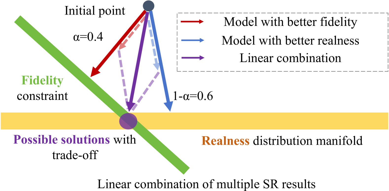
Figure 1: Illustration for vector decomposition in the image super-resolution process. It shows the simple linear approach, which serves as the motivation of our proposed CTSR.

1 Introduction

Image restoration, particularly image super-resolution (SR), is both a critical and challenging task in image processing. Early research [66, 29, 59] typically focused on fixed degradation operators, such as downsampling and blur kernels, modeled as $\mathbf{y}=\mathbf{Ax}+\mathbf{n}$, where $\mathbf{x}$ represents the original image, $\mathbf{A}$ is the fixed degradation operator, $\mathbf{n}$ is random noise, and $\mathbf{y}$ is the degraded result. As the field has advanced, more recent work has shifted its focus to real-world degradation scenarios, where $\mathbf{A}$ turns to a complex and random combination of various degradations, with unknown degradation types and parameters. The evaluation of image super-resolution is mainly based on two metrics: fidelity, which measures the consistency between the super-resolved image and the degraded image, and realness, which assesses how well the super-resolved image conforms to the prior distribution of natural images, as well as its visual quality [38, 80, 75].

The early methods primarily used architectures based on GAN [14] and MSE, trained on pairs of original and degraded images [10, 32, 54, 15]. These approaches excelled in achieving good fidelity in super-resolved results but often suffered from over-smoothing and detail loss [4]. The introduction of diffusion models brought powerful visual priors to the SR task, significantly improving the realness and visual quality of super-resolved images. However, these models frequently struggle with maintaining consistency between the super-resolved and degraded images. Achieving a satisfactory balance between fidelity and realness remains a challenge, with most methods failing to strike an effective trade-off.

Our insight is inspired by the simple attempt at linear combination. Let the super-resolved result with good fidelity be $\mathbf{x}_{f}$, and the super-resolved result with good realness be $\mathbf{x}_{r}$. By linearly combining them as $\mathbf{x}_{c}=\alpha\mathbf{x}_{f}+(1-\alpha)\mathbf{x}_{r}$, we can manually adjust $\alpha\in[0,1]$ to achieve a better balance between fidelity and realness in the final result $\mathbf{x}_{c}$. Building on the insights from DDS [24], we treat the super-resolution process based on diffusion as a vector in the manifold space [5, 47], from the low-resolution (LR) input to the high-resolution (HR) output. This vector can be geometrically decomposed into two components: (1) convergence toward the natural image distribution using the diffusion prior, ensuring realness, and (2) correction toward consistency constraints, ensuring fidelity. This decomposition is illustrated in Fig. 1.

Motivated by this observation, we propose a controllable trade-off real-world image super-resolution method based on fidelity-realness distillation, which we name CTSR. Our method distills a diffusion-based SR approach with high fidelity to an existing SR model with strong realness, which also serves as a teacher to distill itself, maintaining its superior performance of realness. Furthermore, To achieve a continuous and controllable trade-off, we further distill the model using the flow-matching technique [33, 83, 13], enabling it to freely adjust between fidelity and realness. Specifically, assuming sampling steps range from $0$ to $T$, the distilled model exhibits better fidelity at step $T$, better realness at step $0$, and a trade-off between the two at intermediate steps. Based on this approach, our CTSR enables the controllability of SR results, as shown in Fig. LABEL:fig:teaser. To summarize, our contributions are three-fold:

❑ We propose a real-world image super-resolution method based on fidelity-realness distillation, effectively achieving a trade-off between fidelity and realness.

❑ We further introduce a continuous and controllable trade-off approach through another distillation process, enabling the model to freely adjust the balance between fidelity and realness, thus providing practical user flexibility and advancing the optimization of image SR tasks.

❑ Experiments on real-world image SR benchmarks demonstrate the superior performance of our proposed CTSR method, along with efficient inference sampling steps and reduced trainable parameter count.

2 Related Work

GAN-based and MSE-oriented Image SR Methods Earlier work mainly use GAN [14] and MSE-oriented [51, 10] networks to implement the image SR task [42, 55, 39, 54, 70, 40]. SRGAN [30] first uses the GAN network to image SR task, optimized via both GAN and perceptual losses, to improve visual quality. Based on this observation, ESRGAN [54] improved detail recovery by incorporating a relativistic average discriminator. Methods like BSRGAN [74] and Real-ESRGAN [55] follow the complexities of real-world degradation, allowing the ISR approaches to effectively tackle uncertain degradation, thus improving the flexibility of the model. Although GAN-based methods can inject more realistic detail into images, they struggle with challenges such as training instability. For MSE-oriented methods, SwinIR [32] introduces a strong baseline model for image restorations, which includes image super-resolution (including known degradation and real-world types), image denoising, and JPEG compression artifacts. As this method is also trained in an end-to-end manner, it also faces problems like over-smooth and detail missing.

Diffusion-based Image SR Methods As diffusion models have developed, their strong visual priors have also been applied to image super-resolution tasks. SR3 [45] first proposes a diffusion model for SR task, which uses LR input as the condition of diffusion sampling, thus needs training for the UNet. Further methods like DDRM [27], DDNM [56] and DPS [6] use classifier-free guidance [18], which takes LR input as the guidance of original diffusion sampling; thus, these methods are training-free. However, all these methods are on a fixed degradation setting, where the degradation type and parameters are known.

As these training-free methods use gradient guidance to correct the diffusion sampling process, methods such as DiffBIR [65] and GDP [12] try to leverage the gradient to update the parameters of the degradation operator, and in this case the degradation type is known but the parameters are unknown. Current diffusion-based image SR methods mainly focus on the real-world scenario, where the degradation is unknown and complex [53, 64, 63, 57, 62, 72, 68, 71]. StableSR [53] proposes an image SR method based on Stable Diffusion [43], using an adapter to introduce the LR guidance for diffusion sampling. However, such approach needs multiple steps to obtain SR result, which is time-consuming. ResShift [72] designs a special sampling, accelerating the overall sampling in 15 steps. Currently some methods try to distill the diffusion-based SR methods into one step, including AddSR [64], SinSR [57] and OSEDiff [71]. There are also some papers explore the controllability of diffusion-based SR, including PiSA-SR [50] and OFTSR [83].

3 Preliminaries

Diffuion Probablistic Models [19, 48, 49] are a class of generative models with strong visual prior. The key idea is to model the data distribution by simulating a forward noise-adding process and a reverse denoising process. Let $\mathbf{x}_{0}$ represent the original image, $\mathbf{x}_{t}$ be the data at the t-th step of the forward process. The forward process can be described as: $q(\mathbf{x}_{t}|\mathbf{x}_{t-1})=\mathcal{N}(\mathbf{x}_{t};\sqrt{1-\beta_{t}}\mathbf{x}_{t-1},\beta_{t}\mathbf{I})$, where $\beta_{t}$ controls the noise added at each step, and $\mathcal{N}(\cdot,\boldsymbol{\mu},\sigma^{2}\mathbf{I})$ represents Gaussian distribution with mean $\mu$ and co-variance matrix $\sigma^{2}\mathbf{I}$. The reverse process aims to reconstruct the original data $\mathbf{x}_{0}$ by predicting $\mathbf{x}_{t-1}$ from $\mathbf{x}_{t}$: $p_{\theta}(\mathbf{x}_{t-1}|\mathbf{x}_{t})=\mathcal{N}(\mathbf{x}_{t-1};\boldsymbol{\mu}_{\theta}(\mathbf{x}_{t},t),\sigma_{t}^{2}\mathbf{I})$, where $\boldsymbol{\mu}_{\theta}(\mathbf{x}_{t},t)$ is the predicted mean parameterized by a neural network.

The training of the diffusion model needs a reconstruction loss of the difference between added noise in forward process, and predicted noise in reverse process, formulated as $L=\sum_{t=1}^{T}[||\boldsymbol{\epsilon}_{\theta}(\mathbf{x}_{t},t)-\boldsymbol{\epsilon}||^{2}]$, where $\boldsymbol{\epsilon}_{\theta}(\mathbf{x}_{t},t)$ is the model’s prediction of the noise $\epsilon$ added at each timestep.

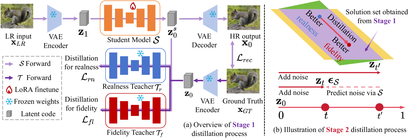
Figure 2: Illustration of our proposed CTSR. (a) At the first stage, we distill student model via two teacher models, one with better fidelity performance, and one with better realness performance. (b) At the second stage, we distill model obtailed from first stage, to a continuous mapping to SR results with different trade-offs between fidelity and realness.

Flow matching [34, 33] is a generative modeling technique similar to diffusion models [37]. It can model and learn the mapping from one data distribution to another through a noise-adding and denoising process, similar to diffusion models. Such distribution transformation process can be applied to tasks such as image reconstruction and style transfer [36, 7, 22, 69].

Convex Optimization for Image Restoration Image restoration, when modeled as $\mathbf{y}=\mathbf{Ax}+\mathbf{n}$, is also known as image inverse problem. The target for image restoration is as $\mathop{\arg\min}\limits_{\mathbf{x}}||\mathbf{y}-\mathbf{Ax}||_{2}^{2}+\lambda\mathcal{R}(\mathbf{x})$, where $\mathcal{R}(\mathbf{x})$ is the regularization term, like $L_{1}$ norm or total variation [44, 82]. This convex optimization problem can be solved via algorithms like gradient descent and ISTA [25], in an iterative process. Take gradient descent step as an example: $\mathbf{x}_{k+1}=\mathbf{x}_{k}+\rho\nabla_{\mathbf{x}}(\mathbf{y}-\mathbf{Ax}_{k})$, where $\mathbf{x}_{k}$ and $\mathbf{x}_{k+1}$ is the restoration result in $k$ and $k+1$ step, and $\rho$ is the learning rate. Diffision-based image SR methods, like DPS [6] and DDS [24], are inspired via such process, taking iterative sampling in diffusion as optimization steps.

4 Method

4.1 Motivation

In diffusion-based methods, some approaches excel in fidelity, such as ResShift [72] and SinSR [57], while others prioritize realness metrics, like OSEDiff [62] and StableSR [53]. Combining the strengths of these methods can facilitate an effective trade-off between the two. One straightforward approach is to linearly combine the super-resolved outputs of different models. For example, by multiplying the image tensor of ResShift by $\alpha$ and OSEDiff by $(1-\alpha)$, and then summing them, both fidelity and realness metrics can be improved by adjusting the coefficients. We validate this on the Nikon test subset of RealSR [2], with the results shown in Tab. 1. We further interpret this linear combination method as the sum of vectors corresponding to different SR methods in image space, as illustrated in Fig. 1.

Settings	PSNR$\uparrow$	LPIPS$\downarrow$	Inference time (s)
$\alpha=0$	24.54	0.3575	0.7546
$\alpha=0.2$	24.84	0.3525	0.9196
$\alpha=0.4$	25.25	0.3633	0.9196
$\alpha=0.6$	25.34	0.3742	0.9196
$\alpha=0.8$	25.10	0.3857	0.9196
$\alpha=1.0$	24.88	0.3915	0.1791
Ours	25.45	0.3411	0.1791

Table 1: Results of the linear combination on RealSR [2] Nikon sub-testset. $\alpha$ is multiplied with ResShift [72], and $(1-\alpha)$ with OSEDiff [62]. By adding SR results from two models, the performance for both fidelity and realness is improved. Best and second-best results shown in red and blue.

However, the performance of the linear combination method above is limited, and its inference speed is slower due to the need to run two models. To address these issues and enhance the model’s representation capability, we extend it to a more general framework. Inspired by the success of knowledge distillation in image SR [23, 78, 79, 81], we distill the model output to the intersection of consistency constraints and high-quality image distribution manifolds, striking a trade-off of fidelity and realness. To further enable controllability of the trade-off between fidelity and realness, we distill the diffusion sampling process of the model into a transformation from realness to fidelity, allowing for a flexible, controllable adjustment between the two. As a result, users can freely adjust these two properties according to their preferences in practical scenarios.

4.2 Overview

Our model is an one-step diffusion-based SR approach finetuned from OSEDiff [62]. The training scheme consists of two stages. In the first stage, as shown in Fig. 2(a), we select an SR model with good realness as the student model $\mathcal{S}$. This model is distilled via LoRA [21] using two teacher models: one with high fidelity (denoted as $\mathcal{T}_{f}$) and another with good realness (denoted as $\mathcal{T}_{r}$). The teacher model $\mathcal{T}_{f}$ guides the student model $\mathcal{S}$ with gradient directions for fidelity, while $\mathcal{T}_{r}$ ensures that the student model retains its original generative capability. As a result, the super-resolution process of the model receives gradient corrections in the fidelity direction, and converges to the intersection of the fidelity constraint and the realness distribution manifold.

In the second stage, as shown in Fig. 2(b), we further distill $\mathcal{S}$ within the solution set obtained from the first stage. Since the diffusion model can be viewed as a distribution transformation mapping from the initial input to the final output, we set the starting point as the super-resolved result from the first stage, with the target transformation being the solution with better fidelity within the solution set. This distribution transformation is achieved through distillation. As the time step $t$ of the diffusion model is continuous, we can controllably select the appropriate trade-off state, allowing us to achieve better and more diverse super-resolution results. An illustration of our proposed CTSR is shown in Fig. 2.

4.3 Stage 1: Distillation via Dual-Teacher Learning

Motivated by the insight in Sec. 4.1, we propose a distillation-based method, where two super-resolution models with good fidelity, $\mathcal{T}_{f}$, and realness, $\mathcal{T}_{r}$, are used to distill the original model $\mathcal{S}$. Our training objective consists of two components:

Reconstruction Loss. The output of the student model should be consistent with the original model in terms of both consistency and visual quality. We choose $L_{2}$ loss and LPIPS loss as the reconstruction loss terms:

$$\mathcal{L}_{rec}=\lambda_{l2}||\mathcal{S}(\mathbf{x}_{LR})-\mathbf{x}_{GT}||_{2}^{2}+\lambda_{lp}\ell(\mathcal{S}(\mathbf{x}_{LR}),\mathbf{x}_{GT})$$ (1)

, where $\mathbf{x}_{LR}$ is input LR image, $\mathbf{x}_{GT}$ is ground-truth image, $\ell$ is LPIPS loss, $\lambda_{l2}$ and $\lambda_{lp}$ are balancing hyper-parameters.

Dual Teacher Distillation Loss. For ease of implementation, we use the same model for both the realness teacher $\mathcal{T}_{r}$ and the student model $\mathcal{S}$. This allows us to split the distillation process into two parts: (1) The fidelity teacher model $\mathcal{T}_{f}$ guides the gradients of $\mathcal{S}$, adjusting its output distribution toward a more faithful direction. (2) The realness teacher model $\mathcal{T}_{r}$ regulates the student model, ensuring that the directional correction in (1) does not deviate from the manifold of the true image distribution achieved by $\mathcal{T}_{r}$. The specific formula for $\mathcal{L}_{fl}$ is as follows:

$$\mathcal{L}_{fl} =||\boldsymbol{\epsilon}_{\mathcal{T}_{f}}\left(\mathbf{z}_{t}^{s},t,c\right)-\boldsymbol{\epsilon}_{\mathcal{S}}\left(\mathbf{z}_{t}^{s},t,c\right)||_{2}^{2}$$ (2)

$$+\gamma_{time}||\boldsymbol{\epsilon}_{\mathcal{T}_{f}}\left(\mathbf{z}^{s}_{t},t,c\right)-\boldsymbol{\epsilon}_{\mathcal{T}_{f}}\left(\mathbf{z}_{t},t,c\right)||_{2}^{2},$$

where $\boldsymbol{\epsilon}_{\mathcal{T}_{f}}$ and $\boldsymbol{\epsilon}_{\mathcal{S}}$ represent the denoising UNet of $\mathcal{T}_{f}$ and $\mathcal{S}$, respectively; $c$ is prompt embedding; $\mathbf{z}_{t}$ and $\mathbf{z}^{s}_{t}$ are the latent codes of ground-truth $\mathbf{x}_{GT}$ and the student model’s SR result $\mathbf{x}_{0}$, obtained via VAE encoder $\mathcal{E}$, each added with the noise at timestep $t$ in the forward process of the diffusion model; $\gamma_{time}$ is the hyperparameter for balancing the two terms. The first term $\boldsymbol{\epsilon}_{\mathcal{T}_{f}}\left(\mathbf{z}_{t}^{s},t,c\right)-\boldsymbol{\epsilon}_{\mathcal{S}}\left(\mathbf{z}_{t}^{s},t,c\right)$ aligns the output of $\mathcal{S}$ with the teacher model $\mathcal{T}_{f}$, enabling the student model to learn the distribution information from the teacher. The second term, $\boldsymbol{\epsilon}_{\mathcal{T}_{f}}\left(\mathbf{z}^{s}_{t},t,c\right)-\boldsymbol{\epsilon}_{\mathcal{T}_{f}}\left(\mathbf{z}_{t},t,c\right)$, leverages the teacher model’s prior to align the SR result $\mathbf{x}_{0}$ with $\mathbf{x}_{GT}$. Since the alignment in the second term is achieved by adding noise to the latent codes of $\mathbf{x}_{0}$ and $\mathbf{x}_{GT}$ separately, and calculating the difference in the predicted noise of $\mathcal{T}_{f}$, it reflects the distributional difference between them in the image space. As a result, compared to directly using $L_{2}$ loss, this approach better captures the distributional differences between the student model and the ground truth, avoiding issues like over-smoothing and loss of detail typically introduced by $L_{2}$ loss, while preserving the semantic details of the original image. We depict the detailed calculating process of $\mathcal{L}_{fl}$ in Supplementary Materials.

This design is similarly applied for the distillation of $\mathcal{T}_{r}$:

$$\mathcal{L}_{rn} =||\boldsymbol{\epsilon}_{\mathcal{T}_{r}}\left(\mathbf{z}_{t}^{s},t,c\right)-\boldsymbol{\epsilon}_{\mathcal{S}}\left(\mathbf{z}_{t}^{s},t,c\right)||_{2}^{2}$$ (3)

$$+\gamma_{time}||\boldsymbol{\epsilon}_{\mathcal{T}_{r}}\left(\mathbf{z}^{s}_{t},t,c\right)-\boldsymbol{\epsilon}_{\mathcal{T}_{r}}\left(\mathbf{z}_{t},t,c\right)||_{2}^{2},$$

By combining these losses, the student model $\mathcal{S}$ can achieve improved fidelity without sacrificing its original performance. As a result, the linear combination method discussed in Sec. 4.1 is extended to a more general approach, where the student’s convergence direction evolves from a simple vector sum to a more precise optimal solution direction. This distillation mechanism is inspired by the SDS [41] and VSD [60, 11] losses, which regulate the student model using both the teacher model and the ground truth.

The loss function for distillation in the first stage is:

$$\mathcal{L}_{s1}=\mathcal{L}_{rec}+\lambda_{rn}\mathcal{L}_{rn}+\lambda_{fl}\mathcal{L}_{fl},$$ (4)

where $\lambda_{rn}$ and $\lambda_{rn}$ are balancing weights.

In short, our proposed distillation method guides student model $\mathcal{S}$ toward the intersection of the fidelity constraint and the realness distribution. The distilled SR model then serves as the teacher model in the following second stage, providing SR solutions with fidelity-realness trade-off.

Datasets	Method	PSNR $\uparrow$	SSIM $\uparrow$	LPIPS $\downarrow$	DISTS $\downarrow$	FID $\downarrow$	NIQE $\downarrow$	MUSIQ $\uparrow$	MANIQA $\uparrow$	CLIPIQA $\uparrow$
	RealESRGAN [55]	28.62	0.8052	0.5428	0.2374	171.79	7.8675	54.26	0.5202	0.4515
	ResShift [72]	28.69	0.7874	0.3525	0.2541	176.77	7.8762	52.40	0.4756	0.5413
	SinSR [57]	28.38	0.7497	0.3669	0.2484	172.72	6.9606	55.03	0.4904	0.6412
DRealSR	CTSR (t=0.8) (ours)	28.47	0.8056	0.3561	0.2369	161.24	7.8462	58.76	0.5453	0.6745
	RealESRGAN [55]	25.69	0.7614	0.3266	0.1646	168.02	4.0146	60.36	0.3934	0.4495
	ResShift [72]	26.39	0.7567	0.3158	0.2432	149.59	6.8746	60.22	0.5419	0.5496
	SinSR [57]	26.27	0.7351	0.3217	0.2341	137.59	6.2964	60.76	0.5418	0.6163
RealSR	CTSR (t=0.2) (ours)	26.29	0.7211	0.3210	0.1620	127.67	4.2979	66.84	0.6314	0.6435
	RealESRGAN [55]	24.29	0.6372	0.3570	0.1621	46.31	3.4591	61.05	0.3830	0.5276
	ResShift [72]	24.71	0.6234	0.3473	0.2253	42.01	6.3615	60.63	0.5283	0.5962
	SinSR [57]	24.41	0.6018	0.3262	0.2068	35.55	5.9981	62.95	0.5430	0.6501
DIV2K-Val	CTSR (t=0.2) (ours)	24.45	0.6098	0.3384	0.1394	24.75	3.6803	69.25	0.5826	0.6726

Table 2: Quantitative comparison with the state-of-the-art (SOTA) methods, which have superior performance on fidelity. “Ours-t” here is chosen as the results when timestep is set as $t$. The best and second-best results of each metric are highlighted in red and blue.

Datasets	Method	PSNR $\uparrow$	SSIM $\uparrow$	LPIPS $\downarrow$	DISTS $\downarrow$	FID $\downarrow$	NIQE $\downarrow$	MUSIQ $\uparrow$	MANIQA $\uparrow$	CLIPIQA $\uparrow$
	StableSR [53]	28.04	0.7454	0.3279	0.2272	144.15	6.5999	58.53	0.5603	0.6250
	DiffBIR [65]	25.93	0.6525	0.4518	0.2761	177.04	6.2324	65.66	0.6296	0.6860
	SUPIR [71]	25.09	0.6460	0.4243	0.2795	169.48	7.3918	58.79	0.5471	0.6749
	PASD [68]	27.79	0.7495	0.3579	0.2524	171.03	6.7661	63.23	0.5919	0.6242
	InvSR [73]	26.75	0.6870	0.4178	0.2144	142.98	6.7030	63.92	0.5439	0.6791
	OSEDiff [62]	27.35	0.7610	0.3177	0.2365	141.93	7.3053	63.56	0.5763	0.7053
DRealSR	CTSR (t=0.0) (ours)	27.38	0.7767	0.3423	0.1937	142.52	6.6438	64.70	0.6412	0.7060
	StableSR [53]	24.62	0.7041	0.3070	0.2156	128.54	5.7817	65.48	0.6223	0.6198
	DiffBIR [65]	24.24	0.6650	0.3469	0.2300	134.56	5.4932	68.35	0.6544	0.6961
	SUPIR [71]	23.65	0.6620	0.3541	0.2488	130.38	6.1099	62.09	0.5780	0.6707
	PASD [68]	25.68	0.7273	0.3144	0.2304	134.18	5.7616	68.33	0.6323	0.5783
	InvSR [73]	24.50	0.7262	0.2872	0.1624	148.16	4.2189	67.45	0.6636	0.6918
	OSEDiff [62]	23.94	0.6736	0.3172	0.2363	125.93	6.3822	67.52	0.6187	0.7001
RealSR	CTSR (t=0.0) (ours)	25.70	0.6962	0.3058	0.1530	121.30	4.0662	67.94	0.6367	0.6495
	StableSR [53]	23.27	0.5722	0.3111	0.2046	24.95	4.7737	65.78	0.6164	0.6753
	DiffBIR [65]	23.13	0.5717	0.3469	0.2108	33.93	4.6056	68.54	0.6360	0.7125
	SUPIR [71]	22.13	0.5279	0.3919	0.2312	31.40	5.6767	63.86	0.5903	0.7146
	PASD [68]	24.00	0.6041	0.3779	0.2305	39.12	4.8587	67.36	0.6121	0.6327
	InvSR [73]	23.32	0.5901	0.3657	0.1370	28.85	3.0567	68.97	0.6122	0.7198
	OSEDiff [62]	23.72	0.6109	0.3058	0.2138	26.34	5.3903	65.27	0.5838	0.6558
DIV2K-Val	CTSR (t=0.0) (ours)	24.34	0.6093	0.3377	0.1377	24.56	3.5455	69.52	0.5894	0.6741

Table 3: Quantitative comparison with SOTA methods having better performance on realness. “Ours-0.0” here denotes the result when timestep of CTSR is set as $0$. The best and second-best results of each metric are highlighted in red and blue, respectively.

4.4 Stage 2: Distillation for Controllablility

As shown in Fig. 1, we represent the optimal solution as a point within a set of feasible solutions obtained from from Sec. 4.3. Within this set, some solutions exhibit better realness, while others demonstrate superior fidelity. Let the possible solutions be denoted as $\mathbf{x}_{0}$ and $\mathbf{x}_{1}$, where $\mathbf{x}_{0}$ performs better in realness and $\mathbf{x}_{1}$ excels in fidelity. These solutions can be viewed as distinct points in the high-dimensional space (where the image domain is considered as a $channel\times height\times width$ space), each at varying distances from the degradation constraint and the ground truth distribution manifold.

Building on the flow matching approach [33, 83], we further distill $\mathcal{S}$, mapping the diffusion sampling process from $\mathbf{x}_{0}$ to $\mathbf{x}_{1}$ within the feasible solution set. The input timesteps $t$ for the diffusion UNet in this mapping act as an adjustable parameter, enabling a a continuous, controllable trade-off between fidelity and realness.

Our training approach involves adding different noise to $\mathbf{z}_{0}$, the latent code of $\mathbf{x}_{0}$, and fine-tuning the denoising UNet $\boldsymbol{\epsilon}_{\mathcal{S}}$. The noise addition process, starting from $t=0$, is as follows:

$$\mathbf{z}_{t}=\mathbf{z}_{0}+t\boldsymbol{\epsilon}_{\mathcal{T}_{S}}(\mathbf{z}_{0},t,c),$$ (5)

where $\mathcal{T}_{S}$ denotes the student model obtained from the first stage. This process also applies for timesteps starting at $t$:

$$\mathbf{z}_{t^{\prime}}=\mathbf{z}_{t}+(\Delta t)\boldsymbol{\epsilon}_{\mathcal{T}_{S}}(\mathbf{z}_{0},t,c),$$ (6)

where $\Delta t=t^{\prime}-t$. The student model $\mathcal{S}$ should adhere to the following equation:

$$t^{\prime}\epsilon_{\mathcal{T}_{S}}(\mathbf{z}_{0},t^{\prime},c)-t\epsilon_{\mathcal{T}_{S}}(\mathbf{z}_{0},t,c)=(\Delta t)\epsilon_{\mathcal{S}}(\mathbf{z}_{t},t,c),$$ (7)

wher the left-hand term represents the difference in added noise to latent code, and the right-hand term is the predicted noise by the student model $\mathcal{S}$. To satisfy the requirement in Eq. 7, $\mathcal{S}$ is finetuned using the following loss:

$$\mathcal{L}_{ctrl_{t,t^{\prime}}} =||t\boldsymbol{\epsilon}_{\mathcal{T}_{s}}(\mathbf{z}_{0},t,c)-t^{\prime}\boldsymbol{\epsilon}_{\mathcal{T}_{s}}(\mathbf{z}_{0},t^{\prime},c)$$ (8)

$$+(\Delta t)\boldsymbol{\epsilon}_{\mathcal{S}}(\mathbf{z}_{t},t,c)||_{2}^{2},$$

where $t$ and $t^{\prime}$ are uniformly sampled from the range 0 to 1, separately. The overall loss function for controllable trade-off distillation in the second stage is then:

$$\mathcal{L}_{s2}=\mathcal{L}_{ctrl_{t,t^{\prime}}},\;t,t^{\prime}\in(0,1).$$ (9)

By randomly sampling the timesteps $t$ and $t^{\prime}$, the student model gradually learns the distribution of the first-stage solution set, acquiring information about solutions with better fidelity. Due to the inherent uncertainty and diversity in the noise addition and UNet predictions during distillation, our model efficiently utilizes the diversity of the diffusion model in SR tasks.

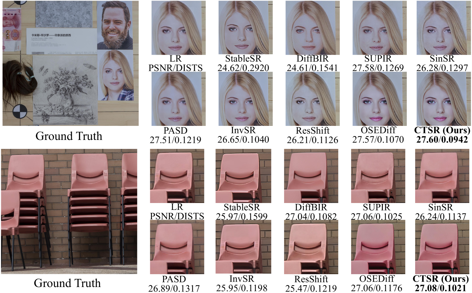
Figure 3: Visualized results of evaluation on the RealSR testset, with our proposed CTSR ($t=0.0$) and compared methods.

5 Experiments

5.1 Settings

Datasets We merge the training sets from DIV2K [1], LSDIR [31], DRealSR [61], ImageNet [8], and RealSR [2] as our training dataset, and evaluate our method on the validation sets of DIV2K, DRealSR, and RealSR. Degraded images are generated using the real-world degradation operator from RealESRGAN [55].

Evaluation Metrics We assess both fidelity and realness for the super-resolution task. For fidelity, we use PSNR and SSIM [58]; for realness, we use LPIPS [77], DISTS [9], and FID [17], which require reference images, and NIQE [76], MUSIQ [28], CLIPIQA [52], and MANIQA [67], which are reference-free. LPIPS uses VGG [46] weights following  [11], and MANIQA uses PIPAL [26] weights by default.

Implementation Details For the teacher model selection, we choose OSEDiff [62] as $\mathcal{T}_{r}$, due to its advantage in realness, and ResShift [72] as$\mathcal{T}_{r}$, for its better fidelity performance. The pretrained version of Stable Diffusion [43] used is 2.1-base. The default image input size for the models is 512$\times$512. All images are processed at their original size, and for images larger than 512$\times$512, we use patch splitting and apply VAE tiling to avoid block artifacts. In both the first and second stages of training, we use the AdamW [35] optimizer with $\beta_{1}$=0.9, $\beta_{2}$=0.999, and a learning rate of 5e-5, with 20,000 training steps in the first stage and 50,000 in the second stage. The batch size is set to 1. Distilltion in both stages is performed using LoRA [21] fine-tuning, with a rank of 4. For the loss balancing coefficients in $\mathcal{L}_{s1}$, $\lambda_{rn}$ is set to 1, $\lambda_{fl}$ to 2, and $\gamma_{time}$ to 5.5. In $\mathcal{L}_{rec}$, $\lambda_{l2}$ and $\lambda_{lp}$ are set to 1 and 2 respectively. All experiments are conducted on SR task with a scaling factor of 4, using an NVIDIA A6000 GPU.

5.2 Comparison with State-of-the-arts

Comparison Methods. We select methods for comparison based on two performance metrics: fidelity and realness, and group them accordingly. For fidelity, we choose ResShift [72], SinSR [57], and RealESRGAN [55]; for realness, we select StableSR [53], DiffBIR [65], SUPIR [71], SinSR [57], PASD [68], InvSR [73], and OSEDiff [62].

Loss type	PSNR$\uparrow$	SSIM$\uparrow$	LPIPS$\downarrow$	CLIPIQA$\uparrow$	MANIQA$\uparrow$
w/o distill	26.71	0.6743	0.4552	0.5439	0.5775
w/ distill (Ours)	25.70	0.6962	0.3058	0.6495	0.6367

Table 4: Ablation of training with and without dual teacher distillation loss. Best results are shown in red.

Teacher $\mathcal{T}_{fl}$	PSNR$\uparrow$	SSIM$\uparrow$	LPIPS$\downarrow$	CLIPIQA$\uparrow$	MANIQA$\uparrow$
SinSR	25.71	0.6734	0.3552	0.6036	0.6065
ResShift (Ours)	25.70	0.6962	0.3058	0.6495	0.6367

Table 5: Results of different choices on $\mathcal{T}_{fl}$, evaluated on the RealSR testset. Best results are shown in red.

$\lambda_{rn}$	PSNR$\uparrow$	LPIPS$\downarrow$	$\lambda_{fl}$	PSNR$\uparrow$	LPIPS$\downarrow$	$\gamma_{time}$	PSNR$\uparrow$	LPIPS$\downarrow$
0.6	25.07	0.3487	1.6	25.81	0.3377	4.5	25.08	0.3481
0.8	24.81	0.3185	1.8	25.62	0.3365	5.0	25.60	0.3166
1.0	25.70	0.3058	2.0	25.70	0.3058	5.5	25.70	0.3058
1.2	25.66	0.3376	2.2	25.44	0.3149	6.0	24.82	0.3212
1.4	25.62	0.3317	2.4	25.19	0.3226	6.5	27.07	0.3490

Table 6: Ablation for $\lambda_{rn}$, $\lambda_{fl}$ and $\lambda_{time}$. It is shown that our choice (in bold) leads to a better trade-off for both fidelity and realness. Best and second-best results shown in red and blue.

Timestep $t$	PSNR$\uparrow$	LPIPS$\downarrow$	NIQE$\downarrow$	MUSIQ$\uparrow$
0.0	24.34	0.3377	3.5455	69.52
0.2	24.45	0.3384	3.6803	69.25
0.4	24.58	0.3397	3.8114	69.00
0.6	24.72	0.3409	3.9368	68.60
0.8	24.82	0.3423	4.0234	68.25
1.0	24.85	0.3437	4.0438	67.96

Table 7: Results of the controllable trade-off between fidelity and realness, with adjustable properties implemented via timestep $t$. Test on the DIV2K validation set. Best results shown in red.

	StableSR [53]	DiffBIR [65]	SUPIR [71]	PASD [68]	ResShift [72]	InvSR [73]	SinSR [57]	OSEDiff [62]	Ours
Inference Step	200	50	50	20	15	1	1	1	1
Inference Time (s)	12.4151	7.9637	16.8704	4.8441	0.7546	0.1416	0.1424	0.1791	0.1791
Total / Trainable Parameters (M)	1410 / 150.0	1717 / 380.0	2662.4 / 1331.2	1900 / 625.0	110 / 118.6	1010 / 33.8	119 / 118.6	1775 / 8.5	1775 / 8.5

Table 8: Comparison of computational complexity, training time, and number of trainable parameters across diffusion-based methods. Loading time for model weights and dataloaders are not included. Best and second-best results are shown in red and blue.

Method	PSNR$\uparrow$	SSIM$\uparrow$	LPIPS$\downarrow$	Parameters (M) $\downarrow$
GSAD [20]	28.67	0.9444	0.0487	17.17
Reti-Diff [16]	27.53	0.9512	0.0349	26.11
GSAD (Distilled)	28.69	0.9507	0.0336	17.17

Table 9: Our distillation applied in low-light enhancement task evaluated on LOL-v2-syn [3] testset, which brings fidelity preservation and realness improvement. Best results shown in red.

Quantitative Comparison. We use RealESRGAN as a simulation of real-world degradation and compare the performance on the DIV2K, RealSR, and DRealSR validation sets. Tab. 2 and Tab. 3 present the quantitative comparison results.

Tab. 2 compares our method with existing methods that excel in terms of fidelity, showing that our method is comparable in terms of PSNR and SSIM, while significantly outperforming others on realness metrics such as DISTS, FID, and others. The comparison with RealESRGAN further demonstrates that diffusion-based methods generally achieve higher scores on no-reference metrics (NIQE, MANIQA, CLIPIQA, MUSIQ), suggesting that diffusion models are better suited to provide visual priors for super-resolution tasks.

Tab. 3 compares our method with existing methods that excel in realness. The results show that our method is competitive in realness metrics, while also achieving significant performance gains in fidelity.

Qualitative Comparison. Fig. 3 presents the results of comparison experiments on the RealSR testset. The figure shows that our method provides better visual quality and consistency with the original image compared to the other methods.

Efficiency Comparison. To evaluate the efficiency and complexity of CTSR, we compare these properties with SOTA methods in Tab. 8, which shows that CTSR requires fewer inference steps, achieves comparable inference time and has fewer trainable parameters.

5.3 Ablation Study

Necessity of Teacher Distillation Loss. A natural question arises: “why do we need two teacher models to achieve the trade-off, given that many methods use $L_{2}$ loss and LPIPS loss for balancing fidelity and realness?”. From a theoretical standpoint, $L_{2}$-norm, when used as the fidelity constraint, is too sparse and lacks the smoothness necessary to capture the detailed semantic information of the LR input. On the other hand, regularization losses like LPIPS struggle to effectively represent the distribution of natural images. By training SR models on a diffusion prior with various strategies, we can obtain better guidance for balancing fidelity and realness, thereby advancing the Pareto frontier of SR tasks. To further support this, we present results with and without the distillation loss in Tab. 4. The comparison shows that without the distillation loss, the method reverts to the behavior of earlier GAN-based approaches, achieving better fidelity but suffering a significant decline in realness and visual quality.

Selection of Teacher $\mathcal{T}_{fl}$. Since multiple SOTA SR models excel in fidelity performance, to find the best choice for $\mathcal{T}_{fl}$, we also experiment with SinSR [57] as the teacher model for dual teacher distillation. The results are presented in Tab. 5.

Selection of Coefficients $\lambda_{fl}$, $\lambda_{rn}$ and $\gamma_{time}$. For the balancing coefficients among the loss function terms, we employ a grid search to determine the values that yield the best overall performance. The results of this selection process are shown in Tab. 6.

5.4 Evaluation of Controllability and Extendability

Contollability. Here, we introduce a controllable image super-resolution method enabled by the second stage of distillation that we propose. Specifically, the controllability of CTSR is determined by the input timestep $t$ of the diffusion model, where where $t=0$ corresponds to the best realness and $t=1$ corresponds to the best fidelity. The input $t$ can be selected anywhere between 0 and 1, allowing the user to adjust the balance between these two properties. We evaluate performance on the DIV2K validation set, with results presented in Tab. 7. As the input timestep $t$ increases from 0 to 1, fidelity metrics such as PSNR and SSIM improve, while realness metrics like LPIPS begin to decrease. Visual results are shown in Fig. LABEL:fig:teaser(a) and Supplementary Materials.

Extension to Image Enhancement. To demonstrate the generalization and versatility of our proposed fidelity-realness distillation method from Sec.  4.3, we extend it to the low-light enhancement (LLE) task, showcasing the performance improvement achieved by this approach. We select two diffusion-based LLE methods: GSAD [20], which excels in fidelity, and Reti-Diff [16], which excels in realness, and apply a training strategy similar to our CTSR. The results, presented in Tab. 9, show that our proposed distillation strategy preserves the fidelity advantage of GSAD while leveraging the model prior from Reti-Diff to enhance realness performance. To be specific, the performance improves by 0.02 in PSNR, 0.0063 in SSIM, and 0.0151 in LPIPS, thus validating the effectiveness and generality of our approach.

6 Conclusion

This paper proposes CTSR, a distillation-based real-world image super-resolution method that leverages multiple teacher models to strike a trade-off between realness and fidelity. Furthermore, inspired by the working pricinple of flow matching, to enable controllability between fidelity and realness, this paper explores a controllable trade-off effect by distilling the output distributions of the aforementioned models, enabling a controllable image super-resolution method that is able to be adjusted via input timestep. Experiments on several real-world image super-resolution benchmarks demonstrate the superior performance of CTSR, compared to other competing methods. Additionally, the proposed fidelity-realness distillation approach can be extended to other tasks like low-light enhancement for performance improvement.

Supplementary Material

In the supplementary materials, we demonstrate additional experimental results, implementation details, discussion, and analysis as follows.

7 More Implementation Details

7.1 More Details of Loss Funtion

We provide a detailed loss calculation process for Stage 1 in the main paper, as shown in Fig. 4.

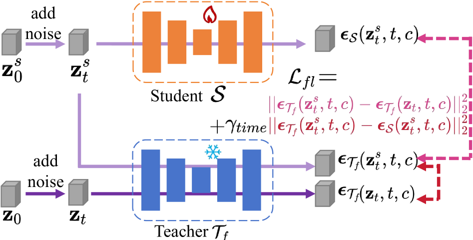
Figure 4: Visualized calculation process of $\mathcal{L}_{fl}$.

7.2 Pseudocode of Our Proposed CTSR Method

The overall training process for first and second stage is shown in Algo. 1 and Algo. 2.

Input: Ground truth $\mathbf{x}_{GT}$, input LR image $\mathbf{x}_{LR}$, student model $\mathcal{S}$, teacher model $\mathcal{T}_{fl}$ and $\mathcal{T}_{rn}$, VAE encoder $\mathcal{E}$, VAE decoder $\mathcal{D}$, embedding of prompt $c$, loss balancing hyper-parameters $\lambda_{time}$, $\lambda_{fl}$, $\lambda_{rn}$, $\lambda_{l2}$, $\lambda_{lp}$

Output: Student model $\mathcal{S}$

1 Initialize $\mathcal{S}$ using weight of $\mathcal{T}_{rn}$.

2 for $epoch=1$ to $total\;epochs$ do

3    $\mathbf{z}_{1}=\mathcal{E}(\mathbf{x}_{LR})$

4    $\mathbf{z}_{0}=\mathcal{E}(\mathbf{x}_{GT})$

5    Random sample a timestep $t$

6    $\mathbf{z}_{t}=add\_noise(\mathbf{z}_{0},t)$

7    $\mathbf{z}_{0}^{s}=\mathcal{S}(\mathbf{z}_{1})$

8    $\mathbf{x}_{0}=\mathcal{D}(\mathbf{z}_{0}^{s})$

9    $\mathbf{z}_{t}^{s}=add\_noise(\mathbf{z}_{0}^{s},t,c)$

10    $\mathcal{L}_{rec}=\lambda_{l2}||\mathbf{x}_{GT}-\mathbf{x}_{0}||_{2}^{2}+\lambda_{lp}\ell(\mathbf{x}_{GT},\mathbf{x}_{0})$

11    $\mathcal{L}_{fl}=||\boldsymbol{\epsilon}_{\mathcal{T}_{f}}(\mathbf{z}_{t}^{s},t,c)-\boldsymbol{\epsilon}_{\mathcal{S}}(\mathbf{z}_{t}^{s},t,c)||_{2}^{2}+\lambda_{time}||\boldsymbol{\epsilon}_{\mathcal{T}_{f}}(\mathbf{z}_{t},t,c)-\boldsymbol{\epsilon}_{\mathcal{T}_{f}}(\mathbf{z}_{t}^{s},t,c)||_{2}^{2}$

12    $\mathcal{L}_{rn}=||\boldsymbol{\epsilon}_{\mathcal{T}_{r}}(\mathbf{z}_{t}^{s},t,c)-\boldsymbol{\epsilon}_{\mathcal{S}}(\mathbf{z}_{t}^{s},t,c)||_{2}^{2}+\lambda_{time}||\boldsymbol{\epsilon}_{\mathcal{T}_{r}}(\mathbf{z}_{t},t,c)-\boldsymbol{\epsilon}_{\mathcal{T}_{r}}(\mathbf{z}_{t}^{s},t,c)||_{2}^{2}$

13    $\mathcal{L}_{s1}=\mathcal{L}_{rec}+\lambda_{fl}\mathcal{L}_{fl}+\lambda_{rn}\mathcal{L}_{rn}$

14    $\mathcal{L}_{s1}.backward()$

15    $\mathcal{S}.update()$

16 end for

return $\mathbf{S}$

Algorithm 1 Fidelity-Realness Distillation in Stage 1

Input: HR output of student model $\mathbf{x}_{0}$, student model $\mathcal{S}$, teacher model (weight initalized from student model) $\mathcal{T}_{\mathcal{S}}$, VAE encoder $\mathcal{E}$

Output: Student model $\mathcal{S}$

1 for $epoch=1$ to $total\;epochs$ do

2    Randomly sample timesteps $t$ and $t^{\prime}$ $\in(0,1)$ /* ensure $t^{\prime}>t$ */

3    $\mathbf{z}_{t}=\mathbf{z}_{0}+t\boldsymbol{\epsilon}_{\mathcal{T}_{\mathcal{S}}}(\mathbf{z}_{0},t,c)$

4    $\mathbf{z}_{t^{\prime}}=\mathbf{z}_{t}+t^{\prime}\boldsymbol{\epsilon}_{\mathcal{T}_{\mathcal{S}}}(\mathbf{z}_{0},t,c)$

5   

6   $\mathcal{L}_{ctrl_{t,t^{\prime}}}=||t\boldsymbol{\epsilon}_{\mathcal{T}_{\mathcal{S}}}(\mathbf{z}_{t},t,c)-t^{\prime}\boldsymbol{\epsilon}_{\mathcal{T}_{\mathcal{S}}}(\mathbf{z}_{t^{\prime}},t^{\prime},c)+(\Delta t)\boldsymbol{\epsilon}_{\mathcal{S}}(\mathbf{z}_{t},t,c)||_{2}^{2}$

7    $\mathcal{L}_{s2}=\sum_{t,t^{\prime}\in[0,1]}\mathcal{L}_{ctrl_{t,t^{\prime}}}$

8    $\mathcal{L}_{s2}.backward()$

9    $\mathcal{S}.update()$

10 end for

return $\mathcal{S}$

Algorithm 2 Controllability Distillation in Stage 2

8 More Experimental Results

8.1 More Results of Controllable Image SR

Here we present the controllable image SR effect on the validation sets of DIV2K, RealSR and DRealSR. Results are shown in Tab. 10, Tab. 11 and Tab. 12 seperately.

Timestep $t$	PSNR$\uparrow$	SSIM$\uparrow$	LPIPS$\downarrow$	DISTS$\downarrow$	FID$\downarrow$	NIQE$\downarrow$	MUSIQ$\uparrow$	MANIQA$\uparrow$	CLIPIQA$\uparrow$
0.0	24.34	0.6093	0.3377	0.1377	24.56	3.5455	69.52	0.5894	0.6741
0.2	24.45	0.6098	0.3384	0.1394	24.75	3.6803	69.25	0.5826	0.6726
0.4	24.58	0.6131	0.3397	0.1412	25.00	3.8114	69.00	0.5767	0.6715
0.6	24.72	0.6172	0.3409	0.1432	25.64	3.9368	68.60	0.5698	0.6684
0.8	24.82	0.6191	0.3423	0.1447	26.13	4.0234	68.25	0.5642	0.6632
1.0	24.85	0.6192	0.3437	0.1459	26.32	4.0438	67.96	0.5609	0.6585

Table 10: More results of the controllable trade-off between fidelity and realness, with adjustable properties implemented via timestep $t$. Test on the DIV2K validation set.

Timestep $t$	PSNR$\uparrow$	SSIM$\uparrow$	LPIPS$\downarrow$	DISTS$\downarrow$	FID$\downarrow$	NIQE$\downarrow$	MUSIQ$\uparrow$	MANIQA$\uparrow$	CLIPIQA$\uparrow$
0.0	25.70	0.6962	0.3058	0.1530	121.30	4.0662	67.94	0.6367	0.6495
0.2	26.29	0.7211	0.3210	0.1620	127.67	4.2979	66.84	0.6314	0.6435
0.4	26.61	0.7203	0.3178	0.1594	134.38	4.2320	66.33	0.6355	0.6340
0.6	26.62	0.7204	0.3191	0.1605	145.21	4.2561	65.29	0.6340	0.6333
0.8	26.65	0.7208	0.3206	0.1614	148.86	4.2708	62.64	0.6327	0.6240
1.0	26.72	0.7213	0.3220	0.1628	156.38	4.3209	61.08	0.6304	0.6209

Table 11: More results of the controllable trade-off between fidelity and realness, with adjustable properties implemented via timestep $t$. Test on the RealSR testset.

Timestep $t$	PSNR$\uparrow$	SSIM$\uparrow$	LPIPS$\downarrow$	DISTS$\downarrow$	FID$\downarrow$	NIQE$\downarrow$	MUSIQ$\uparrow$	MANIQA$\uparrow$	CLIPIQA$\uparrow$
0.0	27.38	0.7767	0.3423	0.1937	142.52	6.6438	64.70	0.6412	0.7060
0.2	27.53	0.7794	0.3446	0.1402	147.25	7.7594	63.52	0.6408	0.7042
0.4	27.99	0.8023	0.3513	0.1687	150.39	7.5088	63.35	0.5654	0.6958
0.6	28.22	0.8043	0.3528	0.2195	156.36	7.5306	62.99	0.5642	0.6930
0.8	28.47	0.8056	0.3561	0.2369	161.24	7.8462	58.76	0.5453	0.6745
1.0	28.68	0.8152	0.3697	0.2371	164.46	7.9699	57.85	0.5974	0.6664

Table 12: More results of the controllable trade-off between fidelity and realness, with adjustable properties implemented via timestep $t$. Test on the DRealSR testset.

8.2 More Visual Results

We provide more results presenting the controllability of our proposed CTSR, which are shown in Fig. 5. From left to right, the fidelity property is gradually changed to realness, with less smooth and more details and better visual quality.

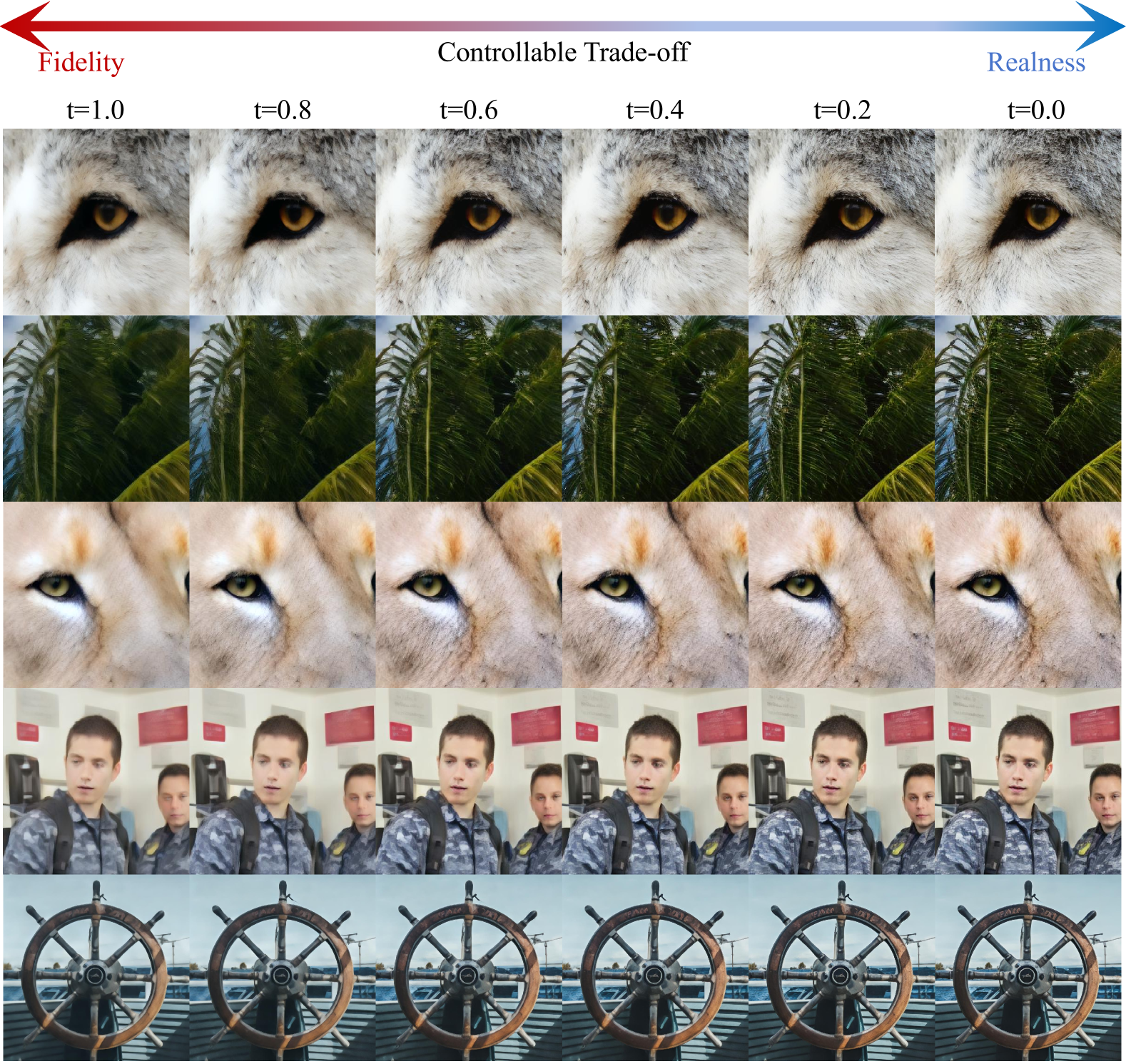
Figure 5: Visualized results of controllable image SR.

References

- Agustsson and Timofte [2017] Eirikur Agustsson and Radu Timofte. Ntire 2017 challenge on single image super-resolution: Dataset and study. In Proceedings of the IEEE conference on computer vision and pattern recognition workshops, pages 126–135, 2017.
- Cai et al. [2019] Jianrui Cai, Hui Zeng, Hongwei Yong, Zisheng Cao, and Lei Zhang. Toward real-world single image super-resolution: A new benchmark and a new model. In Proceedings of the IEEE/CVF international conference on computer vision, pages 3086–3095, 2019.
- Chen et al. [2018] Wei Chen, Wang Wenjing, Yang Wenhan, and Liu Jiaying. Deep retinex decomposition for low-light enhancement. In British Machine Vision Conference, 2018.
- Chen et al. [2024] Yaxin Chen, Huiqian Du, and Min Xie. Ccir: high fidelity face super-resolution with controllable conditions in diffusion models. Signal, Image and Video Processing, 18(12):8707–8721, 2024.
- Chung et al. [2022] Hyungjin Chung, Byeongsu Sim, and Jong Chul Ye. Improving diffusion models for inverse problems using manifold constraints. In Proceedings of the Advances in Neural Information Processing Systems (NeurIPS), 2022.
- Chung et al. [2023] Hyungjin Chung, Jeongsol Kim, Michael Thompson Mccann, Marc Louis Klasky, and Jong Chul Ye. Diffusion posterior sampling for general noisy inverse problems. In Proceedings of the International Conference on Learning Representations (ICLR), 2023.
- Dao et al. [2023] Quan Dao, Hao Phung, Binh Nguyen, and Anh Tran. Flow matching in latent space. arXiv preprint arXiv:2307.08698, 2023.
- Deng et al. [2009] Jia Deng, Wei Dong, Richard Socher, Li-Jia Li, Kai Li, and Li Fei-Fei. Imagenet: A large-scale hierarchical image database. In Proceedings of the IEEE Conference on Computer Vision and Pattern Recognition (CVPR), 2009.
- Ding et al. [2020] Keyan Ding, Kede Ma, Shiqi Wang, and Eero P Simoncelli. Image quality assessment: Unifying structure and texture similarity. IEEE transactions on pattern analysis and machine intelligence, 44(5):2567–2581, 2020.
- Dong et al. [2015] Chao Dong, Chen Change Loy, Kaiming He, and Xiaoou Tang. Image super-resolution using deep convolutional networks. IEEE Transactions on Pattern Analysis and Machine Intelligence (TPAMI), 2015.
- Dong et al. [2024] Linwei Dong, Qingnan Fan, Yihong Guo, Zhonghao Wang, Qi Zhang, Jinwei Chen, Yawei Luo, and Changqing Zou. Tsd-sr: One-step diffusion with target score distillation for real-world image super-resolution. arXiv preprint arXiv:2411.18263, 2024.
- Fei et al. [2023] Ben Fei, Zhaoyang Lyu, Liang Pan, Junzhe Zhang, Weidong Yang, Tianyue Luo, Bo Zhang, and Bo Dai. Generative diffusion prior for unified image restoration and enhancement. In Proceedings of the IEEE/CVF Conference on Computer Vision and Pattern Recognition (CVPR), 2023.
- Fischer et al. [2023] Johannes S Fischer, Ming Gui, Pingchuan Ma, Nick Stracke, Stefan A Baumann, and Björn Ommer. Boosting latent diffusion with flow matching. arXiv preprint arXiv:2312.07360, 2023.
- Goodfellow et al. [2014] Ian Goodfellow, Jean Pouget-Abadie, Mehdi Mirza, Bing Xu, David Warde-Farley, Sherjil Ozair, Aaron Courville, and Yoshua Bengio. Generative adversarial nets. In Proceedings of the Advances in Neural Information Processing Systems (NeurIPS), 2014.
- Guo et al. [2022] Baisong Guo, Xiaoyun Zhang, Haoning Wu, Yu Wang, Ya Zhang, and Yan-Feng Wang. Lar-sr: A local autoregressive model for image super-resolution. In Proceedings of the IEEE/CVF conference on computer vision and pattern recognition, pages 1909–1918, 2022.
- He et al. [2023] Chunming He, Chengyu Fang, Yulun Zhang, Tian Ye, Kai Li, Longxiang Tang, Zhenhua Guo, Xiu Li, and Sina Farsiu. Reti-diff: Illumination degradation image restoration with retinex-based latent diffusion model. In Proceedings of the International Conference on Learning Representations (ICLR), 2023.
- Heusel et al. [2017] Martin Heusel, Hubert Ramsauer, Thomas Unterthiner, Bernhard Nessler, and Sepp Hochreiter. Gans trained by a two time-scale update rule converge to a local nash equilibrium. In Advances in neural information processing systems (NeurIPS), 2017.
- Ho and Salimans [2022] Jonathan Ho and Tim Salimans. Classifier-free diffusion guidance. In Proceedings of the Advances in Neural Information Processing Systems (NeurIPS) Workshop, 2022.
- Ho et al. [2020] Jonathan Ho, Ajay Jain, and Pieter Abbeel. Denoising diffusion probabilistic models. In Proceedings of the Advances in Neural Information Processing Systems (NeurIPS), 2020.
- Hou et al. [2023] Jinhui Hou, Zhiyu Zhu, Junhui Hou, Hui Liu, Huanqiang Zeng, and Hui Yuan. Global structure-aware diffusion process for low-light image enhancement. In Advances in Neural Information Processing Systems (NeurIPS), pages 79734–79747, 2023.
- Hu et al. [2022] Edward J Hu, Yelong Shen, Phillip Wallis, Zeyuan Allen-Zhu, Yuanzhi Li, Shean Wang, Lu Wang, Weizhu Chen, et al. Lora: Low-rank adaptation of large language models. In Proceedings of the International Conference on Learning Representations (ICLR), 2022.
- Hu et al. [2024] Vincent Tao Hu, Wei Zhang, Meng Tang, Pascal Mettes, Deli Zhao, and Cees Snoek. Latent space editing in transformer-based flow matching. In Proceedings of the AAAI conference on artificial intelligence, pages 2247–2255, 2024.
- Hui et al. [2019] Zheng Hui, Xinbo Gao, Yunchu Yang, and Xiumei Wang. Lightweight image super-resolution with information multi-distillation network. In Proceedings of the 27th acm international conference on multimedia, pages 2024–2032, 2019.
- Hyungjin et al. [2024] Chung Hyungjin, Lee Suhyeon, and Ye Jong Chul. Decomposed diffusion sampler for accelerating large-scale inverse problems. In Proceedings of the International Conference on Learning Representations (ICLR), 2024.
- Ito et al. [2019] Daisuke Ito, Satoshi Takabe, and Tadashi Wadayama. Trainable ista for sparse signal recovery. IEEE Transactions on Signal Processing, 67(12):3113–3125, 2019.
- Jinjin et al. [2020] Gu Jinjin, Cai Haoming, Chen Haoyu, Ye Xiaoxing, Jimmy S Ren, and Dong Chao. Pipal: a large-scale image quality assessment dataset for perceptual image restoration. In Proceedings of the European Conference on Computer Vision (ECCV), pages 633–651. Springer, 2020.
- Kawar et al. [2022] Bahjat Kawar, Michael Elad, Stefano Ermon, and Jiaming Song. Denoising diffusion restoration models. In Proceedings of the Advances in Neural Information Processing Systems (NeurIPS), 2022.
- Ke et al. [2021] Junjie Ke, Qifei Wang, Yilin Wang, Peyman Milanfar, and Feng Yang. Musiq: Multi-scale image quality transformer. In Proceedings of the IEEE/CVF international conference on computer vision, pages 5148–5157, 2021.
- Kim and Kwon [2010] Kwang In Kim and Younghee Kwon. Single-image super-resolution using sparse regression and natural image prior. IEEE transactions on pattern analysis and machine intelligence, 32(6):1127–1133, 2010.
- Ledig et al. [2017] Christian Ledig, Lucas Theis, Ferenc Huszár, Jose Caballero, Andrew Cunningham, Alejandro Acosta, Andrew Aitken, Alykhan Tejani, Johannes Totz, Zehan Wang, et al. Photo-realistic single image super-resolution using a generative adversarial network. In Proceedings of the IEEE Conference on Computer Vision and Pattern Recognition (CVPR), 2017.
- Li et al. [2023] Yawei Li, Kai Zhang, Jingyun Liang, Jiezhang Cao, Ce Liu, Rui Gong, Yulun Zhang, Hao Tang, Yun Liu, Denis Demandolx, et al. Lsdir: A large scale dataset for image restoration. In Proceedings of the IEEE/CVF Conference on Computer Vision and Pattern Recognition, pages 1775–1787, 2023.
- Liang et al. [2021] Jingyun Liang, Jiezhang Cao, Guolei Sun, Kai Zhang, Luc Van Gool, and Radu Timofte. Swinir: Image restoration using swin transformer. In Proceedings of the IEEE/CVF International Conference on Computer Vision Workshops (ICCVW), 2021.
- Lipman et al. [2024] Yaron Lipman, Ricky TQ Chen, Heli Ben-Hamu, Maximilian Nickel, and Matt Le. Flow matching for generative modeling. In Advances in neural information processing systems (NeurIPS), 2024.
- Liu et al. [2023] Xingchao Liu, Chengyue Gong, et al. Flow straight and fast: Learning to generate and transfer data with rectified flow. In Proceedings of the International Conference on Learning Representations (ICLR), 2023.
- Loshchilov and Hutter [2017] Ilya Loshchilov and Frank Hutter. Decoupled weight decay regularization. arXiv preprint arXiv:1711.05101, 2017.
- Martin et al. [2024] Ségolène Martin, Anne Gagneux, Paul Hagemann, and Gabriele Steidl. Pnp-flow: Plug-and-play image restoration with flow matching. arXiv preprint arXiv:2410.02423, 2024.
- Meng et al. [2023] Chenlin Meng, Robin Rombach, Ruiqi Gao, Diederik Kingma, Stefano Ermon, Jonathan Ho, and Tim Salimans. On distillation of guided diffusion models. In Proceedings of the IEEE/CVF Conference on Computer Vision and Pattern Recognition, pages 14297–14306, 2023.
- Mentzer et al. [2020] Fabian Mentzer, George D Toderici, Michael Tschannen, and Eirikur Agustsson. High-fidelity generative image compression. In Advances in neural information processing systems, pages 11913–11924, 2020.
- Pan et al. [2021] Xingang Pan, Xiaohang Zhan, Bo Dai, Dahua Lin, Chen Change Loy, and Ping Luo. Exploiting deep generative prior for versatile image restoration and manipulation. IEEE Transactions on Pattern Analysis and Machine Intelligence (TPAMI), 2021.
- Poirier-Ginter and Lalonde [2023] Yohan Poirier-Ginter and Jean-François Lalonde. Robust unsupervised stylegan image restoration. In Proceedings of the IEEE/CVF Conference on Computer Vision and Pattern Recognition (CVPR), 2023.
- Poole et al. [2022] Ben Poole, Ajay Jain, Jonathan T Barron, and Ben Mildenhall. Dreamfusion: Text-to-3d using 2d diffusion. arXiv preprint arXiv:2209.14988, 2022.
- Ren et al. [2020] Haoyu Ren, Amin Kheradmand, Mostafa El-Khamy, Shuangquan Wang, Dongwoon Bai, and Jungwon Lee. Real-world super-resolution using generative adversarial networks. In Proceedings of the IEEE/CVF Conference on Computer Vision and Pattern Recognition Workshops, pages 436–437, 2020.
- Rombach et al. [2022] Robin Rombach, Andreas Blattmann, Dominik Lorenz, Patrick Esser, and Bjorn Ommer. High-resolution image synthesis with latent diffusion models. In Proceedings of the IEEE/CVF Conference on Computer Vision and Pattern Recognition (CVPR), 2022.
- Rudin et al. [1992] Leonid I Rudin, Stanley Osher, and Emad Fatemi. Nonlinear total variation based noise removal algorithms. Physica D: nonlinear phenomena, 60(1-4):259–268, 1992.
- Saharia et al. [2022] Chitwan Saharia, Jonathan Ho, William Chan, Tim Salimans, David J Fleet, and Mohammad Norouzi. Image super-resolution via iterative refinement. IEEE Transactions on Pattern Analysis and Machine Intelligence (TPAMI), 2022.
- Simonyan and Zisserman [2014] Karen Simonyan and Andrew Zisserman. Very deep convolutional networks for large-scale image recognition. arXiv preprint arXiv:1409.1556, 2014.
- Soh et al. [2019] Jae Woong Soh, Gu Yong Park, Junho Jo, and Nam Ik Cho. Natural and realistic single image super-resolution with explicit natural manifold discrimination. In Proceedings of the IEEE/CVF conference on computer vision and pattern recognition, 2019.
- Song et al. [2021] Jiaming Song, Chenlin Meng, and Stefano Ermon. Denoising diffusion implicit models. In Proceedings of the International Conference on Learning Representations (ICLR), 2021.
- Song et al. [2020] Yang Song, Jascha Sohl-Dickstein, Diederik P Kingma, Abhishek Kumar, Stefano Ermon, and Ben Poole. Score-based generative modeling through stochastic differential equations. In Proceedings of the International Conference on Learning Representations (ICLR), 2020.
- Sun et al. [2025] Lingchen Sun, Rongyuan Wu, Zhiyuan Ma, Shuaizheng Liu, Qiaosi Yi, and Lei Zhang. Pixel-level and semantic-level adjustable super-resolution: A dual-lora approach. In Proceedings of the IEEE/CVF Conference on Computer Vision and Pattern Recognition, 2025.
- Vaswani et al. [2017] Ashish Vaswani, Noam Shazeer, Niki Parmar, Jakob Uszkoreit, Llion Jones, AidanN. Gomez, Lukasz Kaiser, and Illia Polosukhin. Attention is all you need. In Proceedings of the Advances in Neural Information Processing Systems (NeurIPS), 2017.
- Wang et al. [2023a] Jianyi Wang, Kelvin CK Chan, and Chen Change Loy. Exploring clip for assessing the look and feel of images. In Proceedings of the AAAI Conference on Artificial Intelligence, pages 2555–2563, 2023a.
- Wang et al. [2024a] Jianyi Wang, Zongsheng Yue, Shangchen Zhou, Kelvin C.K. Chan, and Chen Change Loy. Exploiting diffusion prior for real-world image super-resolution. International Journal of Computer Vision (IJCV), 2024a.
- Wang et al. [2018] Xintao Wang, Ke Yu, Shixiang Wu, Jinjin Gu, Yihao Liu, Chao Dong, Yu Qiao, and Chen Change Loy. Esrgan: Enhanced super-resolution generative adversarial networks. In Proceedings of the European Conference on Computer Vision Workshops (ECCVW), 2018.
- Wang et al. [2021] Xintao Wang, Liangbin Xie, Chao Dong, and Ying Shan. Real-esrgan: Training real-world blind super-resolution with pure synthetic data. In Proceedings of the International Conference on Computer Vision Workshops (ICCVW), 2021.
- Wang et al. [2023b] Yinhuai Wang, Jiwen Yu, and Jian Zhang. Zero-shot image restoration using denoising diffusion null-space model. In Proceedings of the Eleventh International Conference on Learning Representations (ICLR), 2023b.
- Wang et al. [2024b] Yufei Wang, Wenhan Yang, Xinyuan Chen, Yaohui Wang, Lanqing Guo, Lap-Pui Chau, Ziwei Liu, Yu Qiao, Alex C Kot, and Bihan Wen. Sinsr: diffusion-based image super-resolution in a single step. In Proceedings of the IEEE/CVF Conference on Computer Vision and Pattern Recognition (CVPR), 2024b.
- Wang et al. [2004] Zhou Wang, Alan C Bovik, Hamid R Sheikh, and Eero P Simoncelli. Image quality assessment: from error visibility to structural similarity. IEEE transactions on image processing, 13(4):600–612, 2004.
- Wang et al. [2015] Zhaowen Wang, Ding Liu, Jianchao Yang, Wei Han, and Thomas Huang. Deep networks for image super-resolution with sparse prior. In Proceedings of the IEEE international conference on computer vision, pages 370–378, 2015.
- Wang et al. [2023c] Zhengyi Wang, Cheng Lu, Yikai Wang, Fan Bao, Chongxuan Li, Hang Su, and Jun Zhu. Prolificdreamer: High-fidelity and diverse text-to-3d generation with variational score distillation. In Advances in Neural Information Processing Systems (NeurIPS), pages 8406–8441, 2023c.
- Wei et al. [2020] Pengxu Wei, Ziwei Xie, Hannan Lu, Zongyuan Zhan, Qixiang Ye, Wangmeng Zuo, and Liang Lin. Component divide-and-conquer for real-world image super-resolution. In Computer Vision–ECCV 2020: 16th European Conference, Glasgow, UK, August 23–28, 2020, Proceedings, Part VIII 16, pages 101–117. Springer, 2020.
- Wu et al. [2024a] Rongyuan Wu, Lingchen Sun, Zhiyuan Ma, and Lei Zhang. One-step effective diffusion network for real-world image super-resolution. In Proceedings of the Advances in Neural Information Processing Systems (NeurIPS), 2024a.
- Wu et al. [2024b] Rongyuan Wu, Tao Yang, Lingchen Sun, Zhengqiang Zhang, Shuai Li, and Lei Zhang. Seesr: Towards semantics-aware real-world image super-resolution. In Proceedings of the IEEE/CVF Conference on Computer Vision and Pattern Recognition (CVPR), 2024b.
- Xie et al. [2024] Rui Xie, Chen Zhao, Kai Zhang, Zhenyu Zhang, Jun Zhou, Jian Yang, and Ying Tai. Addsr: Accelerating diffusion-based blind super-resolution with adversarial diffusion distillation. arXiv preprint arXiv:2404.01717, 2024.
- Xinqi et al. [2024] Lin Xinqi, He Jingwen, Chen Ziyan, Lyu Zhaoyang, Dai Bo, Yu Fanghua, Ouyang Wanli, Qiao Yu, and Chao Dong. Diffbir: Towards blind image restoration with generative diffusion prior. In Proceedings of the European Conference on Computer Vision (ECCV), 2024.
- Yang et al. [2010] Jianchao Yang, John Wright, Thomas S Huang, and Yi Ma. Image super-resolution via sparse representation. IEEE transactions on image processing, 19(11):2861–2873, 2010.
- Yang et al. [2022] Sidi Yang, Tianhe Wu, Shuwei Shi, Shanshan Lao, Yuan Gong, Mingdeng Cao, Jiahao Wang, and Yujiu Yang. Maniqa: Multi-dimension attention network for no-reference image quality assessment. In Proceedings of the IEEE/CVF Conference on Computer Vision and Pattern Recognition (CVPR), 2022.
- Yang et al. [2024] Tao Yang, Rongyuan Wu, Peiran Ren, Xuansong Xie, and Lei Zhang. Pixel-aware stable diffusion for realistic image super-resolution and personalized stylization. In Proceedings of the European Conference on Computer Vision (ECCV), 2024.
- Yin et al. [2024] Tianwei Yin, Michaël Gharbi, Richard Zhang, Eli Shechtman, Fredo Durand, William T Freeman, and Taesung Park. One-step diffusion with distribution matching distillation. In Proceedings of the IEEE/CVF conference on computer vision and pattern recognition, pages 6613–6623, 2024.
- Yinhuai et al. [2023] Wang Yinhuai, Hu Yujie, Yu Jiwen, and Zhang Jian. Gan prior based null-space learning for consistent super-resolution. In Proceedings of the AAAI Conference on Artificial Intelligence (AAAI), 2023.
- Yu et al. [2024] Fanghua Yu, Jinjin Gu, Zheyuan Li, Jinfan Hu, Xiangtao Kong, Xintao Wang, Jingwen He, Yu Qiao, and Chao Dong. Scaling up to excellence: Practicing model scaling for photo-realistic image restoration in the wild. In Proceedings of the IEEE/CVF Conference on Computer Vision and Pattern Recognition (CVPR), 2024.
- Yue et al. [2023] Zongsheng Yue, Jianyi Wang, and Chen Change Loy. Resshift: Efficient diffusion model for image super-resolution by residual shifting. In Proceedings of the Advances in Neural Information Processing Systems (NeurIPS), 2023.
- Yue et al. [2024] Zongsheng Yue, Kang Liao, and Chen Change Loy. Arbitrary-steps image super-resolution via diffusion inversion. arXiv preprint arXiv:2412.09013, 2024.
- Zhang et al. [2021a] Kai Zhang, Jingyun Liang, Luc Van Gool, and Radu Timofte. Designing a practical degradation model for deep blind image super-resolution. In Proceedings of the IEEE/CVF International Conference on Computer Vision (ICCV), 2021a.
- Zhang et al. [2022] Keke Zhang, Tiesong Zhao, Weiling Chen, Yuzhen Niu, and Jinsong Hu. Spqe: Structure-and-perception-based quality evaluation for image super-resolution. arXiv preprint arXiv:2205.03584, 2022.
- Zhang et al. [2015] Lin Zhang, Lei Zhang, and Alan C Bovik. A feature-enriched completely blind image quality evaluator. IEEE Transactions on Image Processing, 24(8):2579–2591, 2015.
- Zhang et al. [2018] Richard Zhang, Phillip Isola, Alexei A Efros, Eli Shechtman, and Oliver Wang. The unreasonable effectiveness of deep features as a perceptual metric. In Proceedings of the IEEE conference on computer vision and pattern recognition, pages 586–595, 2018.
- Zhang et al. [2021b] Yiman Zhang, Hanting Chen, Xinghao Chen, Yiping Deng, Chunjing Xu, and Yunhe Wang. Data-free knowledge distillation for image super-resolution. In Proceedings of the IEEE/CVF Conference on Computer Vision and Pattern Recognition, pages 7852–7861, 2021b.
- Zhang et al. [2024] Yuehan Zhang, Seungjun Lee, and Angela Yao. Pairwise distance distillation for unsupervised real-world image super-resolution. In European Conference on Computer Vision, pages 429–446. Springer, 2024.
- Zhou and Wang [2022] Wei Zhou and Zhou Wang. Quality assessment of image super-resolution: Balancing deterministic and statistical fidelity. In Proceedings of the 30th ACM international conference on multimedia, pages 934–942, 2022.
- Zhu et al. [2024a] Han Zhu, Zhenzhong Chen, and Shan Liu. Information bottleneck based self-distillation: Boosting lightweight network for real-world super-resolution. IEEE Transactions on Circuits and Systems for Video Technology, 2024a.
- Zhu et al. [2024b] Qiwen Zhu, Yanjie Wang, Shilv Cai, Liqun Chen, Jiahuan Zhou, Luxin Yan, Sheng Zhong, and Xu Zou. Perceptual-distortion balanced image super-resolution is a multi-objective optimization problem. In Proceedings of the 32nd ACM International Conference on Multimedia, pages 7483–7492, 2024b.
- Zhu et al. [2024c] Yuanzhi Zhu, Ruiqing Wang, Shilin Lu, Junnan Li, Hanshu Yan, and Kai Zhang. Oftsr: One-step flow for image super-resolution with tunable fidelity-realism trade-offs. arXiv preprint arXiv:2412.09465, 2024c.