Integral modelling and Reinforcement Learning control of 3D liquid metal coating on a moving substrate
Abstract
Metallic coatings are used to improve the durability of metal surfaces, protecting them from corrosion. These protective layers are typically deposited in a fluid state via a liquid film. Controlling instabilities in the liquid film is crucial for achieving uniform and high-quality coatings. This study explores the possibility of controlling liquid films on a moving substrate using a combination of gas jets and electromagnetic actuators. To model the 3D liquid film, we extend existing integral models to incorporate the effects of electromagnetic actuators. The control strategy was developed within a reinforcement learning framework, where the Proximal Policy Optimization (PPO) algorithm interacts with the liquid film via pneumatic and electromagnetic actuators to optimize a reward function, accounting for the amplitude of the instability waves through a trial and error process. The PPO found an optimal control law, which successfully reduced interface instabilities through a novel control mechanism, where gas jets push crests and electromagnets raise troughs using the Lorentz force.
I Introduction
The interaction between liquid films and external magnetic fields is a relevant physical phenomenon for many engineering applications. Described by magnetohydrodynamic (MHD) equations, this interaction is important for the analysis of magnetic soap films [1], the evaluation of magnetic wiping solutions in dip coating processes [2, 3], the control of mould flow during continuous steel casting [4], and the design of liquid metal films for plasma confinement and heat removal inside nuclear fusion reactors [5, 6].
The complexity of MHD equations poses significant challenges for numerical simulations of these flows [7], often requiring customized software implementations with prohibitive computational costs [8, 9, 10]. To avoid these limitations, Smolentsev and Abdou [11] proposed simplified MHD models based on the long-wave assumption. Other authors used models of reduced-dimensionality with a single evolution equation for film thickness based on depth-averaged equations and a gradient expansion of the velocity components truncated at first or second order [1, 8, 12].
Reduced-dimensional models reproduce the relevant features of the liquid film dynamics with simplified governing equations, which enables analytical analysis and cost-effective computational simulations. Shkadov [13] and Kapitza [14] developed a 2D Integral Boundary Layer (IBL) model for moderate Reynolds number flows in terms of film thickness and flow rate. This model outperformed the single-equation model in capturing the film dynamics. Widely used in the falling liquid film community, a vast spectrum of reduced-dimensional models was developed for different Reynolds and Kapitza numbers of flows, using weighted residual methods and referred to WIBL models (reviewed by Ruyer-Quil et al. [15] and Kalliadasis et al. [16]).
The WIBL model was extended to account for the motion of the substrate and the effect of the pressure gradient and the shear stress distributions on the free surface [17]. Validated against Direct Numerical Simulations (DNS) using the Volume Of Fluid (VOF) technique to track the free surface [18], this enhanced model was used to reproduce the dynamics of the liquid film in the hot-dip galvanizing process with impinging gas jets.
In this process, a metal sheet is coated with a thin layer of zinc by withdrawing it from a bath of molten zinc. The thickness of the final coating is regulated by impinging gas jets, which remove excess liquid from the surface [19, 20]. At withdrawal velocities exceeding 2 m/s, the gas jets oscillate, inducing a liquid film instability known as undulation [20, 21, 22]. This instability manifests itself as nearly 2D travelling waves [18, 23, 24], leading to an uneven coating layer that reduces the quality of the final product, limits the maximum production rate and results in substantial energy and material waste.
A feedback regulator with gas jets and electromagnets represents a possible solution to the undulation problem. Electromagnetic actuators are a new concept recently explored in developing liquid walls for nuclear fusion reactors [25, 26]. Preliminary experiments have shown that a transverse magnetic field can stabilize a liquid film of Galistan flowing over an inclined plate. In an open-loop configuration, Mirhoseini et al. [25] demonstrated the stabilizing effect of a uniform magnetic field. In a closed-loop configuration, they showed that a simple feedback system, using liquid film height observations, can locally stabilize the film by controlling the electric current in the bulk.
This work focuses on closed-loop control of coating non-uniformities in liquid metal films along a moving substrate, using gas jets and electromagnetic actuators with limited free-surface observation points. The optimal control function is developed using Proximal Policy Optimization (PPO) [27], a reinforcement learning (RL) algorithm [28]. RL methods are gaining popularity within the fluid dynamics community across a wide range of applications [29, 30, 31], particularly for high-dimensional control problems with significant noise and uncertainty, as seen in coating control for industrial galvanizing lines. A comparative analysis of RL methods and black-box optimization for flow control is presented in [32]. PPO was used in [33] to stabilize waves in a 2D falling liquid film over an inclined surface, using localized pressure pulsations and limited liquid film thickness observations without relying on knowledge of the governing equations. This work extends the 3D IBL model derived by Ivanova et al. [34], accounting for pneumatic and electromagnetic actuators. Moreover, we investigate the performances of a PPO-trained agent for wave attenuation on a liquid film over a moving substrate.
The rest of the article is structured as follows. Section II outlines the problem and introduces the relevant physical quantities. Section III reviews the reference quantities used to scale the governing equations. The modelling of gas jets and electromagnetic actuators is presented in Section IV. Section V details the numerical methods for solving the reduced-dimensional model equations. Section VII presents the wave dynamics and control performance results. Finally, conclusions and perspectives are discussed in Section VIII.
II Problem description and physical quantities
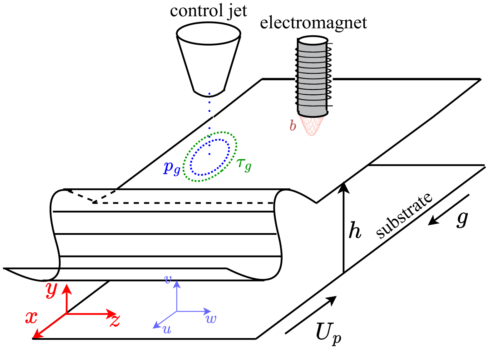
We consider a 3D liquid film of thickness flowing over a substrate moving against gravity at constant speed in contact with air, under the action of external control gas jets and electromagnetic actuators.
For clarity, the physical quantities related to the liquid are written without a subscript, while those related to the air are denoted by the subscript “g”. We consider a liquid film of molten zinc with density , dynamic viscosity , kinematic viscosity , surface tension , electrical conductivity (evaluated at C [35]), magnetic permeability , magnetic diffusivity and magnetic susceptibility where is the magnetic permeability of the void. The air has magnetic permeability and magnetic susceptibility .
For later convenience in the derivation of the reduced-dimensional model, we express the magnetic permeability of the air as a function of the magnetic permeability and susceptibility of the liquid and the magnetic susceptibility of the air through the following relation:
| (1) |
Figure 1 illustrates the coordinate system ; with the axis aligned with the gravity vector pointing downward, the axis pointing along the normal direction of the wall towards the free surface, and the axis spanning the direction of flow, with origin on the substrate. Due to the translational invariance of the problem, specifying a precise origin for the axis is unnecessary.
A local Cartesian coordinate system is defined on the free surface tangent plane as ; , with representing the normal vector pointing towards the air, and and representing the tangential directions along and respectively. These vectors are expressed in (; ) with the following relations:
| (2a) | |||
| (2b) | |||
having used the shorthand notation for partial derivatives, and denotes the transpose of a vector or a matrix.
The film dynamics is described by the velocity field , and the pressure field . The integral formulation of the film dynamics is defined in terms of film thickness and streamwise and spanwise flow rates per unit width, defined as:
| (3) |
Following the modelling approach proposed by Gosset and Buchlin [36] and Mendez et al. [17], the effect of the gas jets at the free-surface is modelled by a pressure and a shear stress distributions.
The influence of the electromagnetic actuator is represented by an external magnetic field , where . Because of the low magnetic susceptibility of both liquid zinc and air , the magnetic fields in the liquid and in the gas , are approximated as being equal to , reading:
| (4a) | |||
| (4b) | |||
The relative motion of the liquid zinc with respect to induces a current in the bulk, denoted as given by Faraday’s law of induction. Neglecting the electric potential difference, as discussed in [37], the induction law reads:
| (5) |
Details on the modelling of , , and are provided in Section IV.
III Integral Modelling with Magnetic Actuators
| Definition | Value | |
| 2 m/s | ||
| 330 m | ||
| 0.583 T | ||
| 102.9 Pa | ||
| 21.87 | ||
| 40 | ||
| Re | 1237 | |
| Ca | 0.01 | |
| 266 | ||
| Ka | 15713 | |
| Ha | 6 | |
| Rm | ||
| S | ||
| N |
This section outlines the derivation of the 3D Integral Boundary Layer (IBL) model, incorporating the effects of gas jets and electromagnetic actuators. The model is presented in dimensionless form, based on the long-wave assumption [16, 15]. Subsection III.1 introduces dimensionless parameters and groups. For conciseness, the complete magnetohydrodynamic equations and boundary conditions are provided in Appendix A. Subsection III.3, introduces the boundary layer equations obtained from the long-wave approximation. Finally, Subsection III.2 discusses the steady-state solutions used to derive the closure relations for the IBL model, presented in Subsection III.4.
III.1 Reference quantities and nondimensional groups
The liquid film governing equations, reported in Appendix A, are scaled as in Ivanova et al. [34], with the addition of two dimensionless numbers accounting for the electromagnetic force. In the following, all dimensionless quantities are denoted with a hat . These are obtained by dividing dimensional variables by their reference quantities, identified by the subscript ‘’. The streamwise and spanwise velocities are scaled by the substrate velocity , and the film thickness is scaled based on the thickness arising from the viscous-gravity balance in steady-state condition [17], namely
| (6) |
The streamwise and the spanwise spatial scales are based on the long wave assumption, which sets:
| (7) |
where is the film parameter, with the capillary number. Based on (6) and (7), the remaining variables are scaled accordingly:
| (8a) | |||
| (8b) | |||
The scaling introduced in Ivanova et al. [34] is expanded by the reference quantities for the magnetic field and the induced current , introduced by the magnetohydrodynamic extension of the model; these are taken as
| (9a) | |||
The capillary number Ca introduced with the definition of the film parameter, can be expressed as , where is the Kapitza number and Re the Reynolds number, which is defined as:
| (10) |
In addition to the Reynolds, Kapitza and capillary numbers, the other non-dimensional groups arising from this scaling are the reduced Reynolds number , the Hartmann number,
| (11) |
the magnetic Reynolds number , the susceptibility ratio and the Stuart number . This number can also be expressed as the ratio of electromagnetic to inertial time scales , where the timescale over which the Lorentz force acts is given by:
| (12) |
where is the spatial scale over which the electromagnetic actuators exert influence.
III.2 Flat-film steady state solution
Before deriving the reduced-dimensional model, it is worth analysing the steady-state flat film solution of the governing equations detailed in Appendix A, excluding the influence of external gas jet actuators. Assuming a stable () and flat () surface, without external shear stress () and no external pressure () distributions, and considering a uniform transversal magnetic field , the flow field becomes parallel () and unidimensional (). The Navier-Stokes equation reduces to the balance of viscous stresses, gravity, and Lorentz force along the streamwise direction :
| (13) |
with the boundary equations (61) and (63) reducing to:
| (14) |
The non-dimensional steady-state velocity of (13) with (14) reads:
| (15) |
with integrating constants and :
| (16a) | |||
| (16b) | |||
III.3 The long wave formulation
In the derivation of the reduced-dimensional model, the liquid film is treated as one-way coupled with the actuators. Moreover, considering the thin film thickness and the negligible magnetic field resulting from the induced current (), it is further assumed that the pressure and shear stress distributions at the free surface are independent of the magnetic field .
The first step in the derivation of the reduced-dimensional model consists in scaling the magnetohydrodynamic equations and the boundary conditions presented in Appendix A using the reference quantities introduced in Subsection III.1. Retaining only terms up to and assuming the surface tension terms and Re to be of , results in the following boundary layer equations:
| (19a) | |||
| (19b) | |||
| (19c) | |||
| (19d) | |||
with boundary conditions:
| (20a) | |||
| (20b) | |||
| (20c) | |||
| (20d) | |||
where represent the normal component of the Maxwell stresses, with and accounting for the gas-jet induced shear stress and the tangential component of the Maxwell stresses at the free surface, reading:
| (21) |
where .
III.4 3D Integral boundary layer model
The integral boundary layer model is derived by integrating the boundary layer equations (19) over the liquid film thickness () using the Leibniz integral rule with the boundary conditions (20). This results in a set of nonlinear hyperbolic partial differential equations in terms of , , and , reading:
| (22) |
where , is the flux matrix defined as:
| (23) |
and is the vector containing the source terms, which is expressed as:
where and with the wall-shear stress vector components along the streamwise and spanwise directions given by:
| (24) |
The convective terms with , along with the wall-shear stress component, are expressed in terms of , , and through closure relations. These relations are based on the assumption of self-similar velocity profile in streamwise and spanwise directions [38, 39]. The shape of these profiles reflects that of the leading-order steady-state solutions given in (15), here concisely rewritten as:
| (25a) | |||
| (25b) | |||
where and the coefficients depend on , , Ha, and . By solving a linear system of equations, which includes the non-slip condition at the substrate (20a), the tangential stress balance at the free surface (20d), and the flow rate definitions (3), the following expressions for these coefficients are derived:
| (26a) | ||||
| (26b) | ||||
| (26c) | ||||
| (26d) | ||||
| (26e) | ||||
| (26f) | ||||
Introducing (25) with the coefficients (26) in the definition of the flux matrix (23) and the wall shear stress (24) gives the following closure relations for the convective flux terms:
| (27a) | |||
| (27b) | |||
| (27c) |
with and for the wall shear stress term , reading:
| (28a) | |||
| (28b) |
Equations (22) with the closure relations (27) and (28) define the 3D IBL model with gas jets and electromagnetic actuators. Considering the conditions relevant to this analysis (see Table 1), we neglect Maxwell stresses as their normal and tangential components appear at in the equations. Despite , and given that , , with derivatives satisfying and , we can confidently neglect these terms.
IV Modelling control actuators
This section outlines the modelling of the gas jet and magnetic forces acting on the liquid film, which are included in the reduced-dimensional model equations (22) and the closure relations (27) and (28) as pressure and shear stress distributions at the free surface and as a wall-normal magnetic field . Pressure and shear stress are modelled using experimental correlations for circular impinging gas jets on a dry substrate (Subsection IV.1). The magnetic field is modelled as a Gaussian distribution, which approximates the magnetic field of a cylindrical electromagnetic actuator (Subsection IV.2).
IV.1 Modelling gas jets actuators
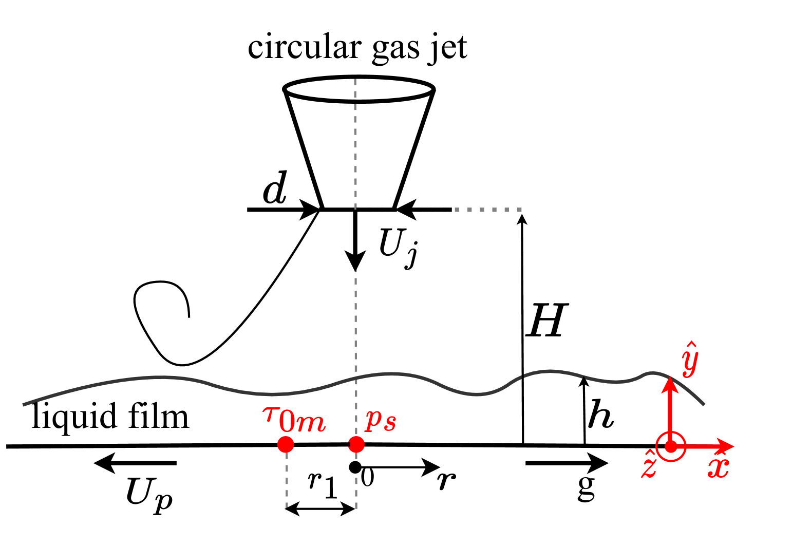
The distribution of pressure and shear stresses on the free surface is modelled using experimental correlations for circular gas jets impinging on a flat dry substrate [40]. Figure 2 provides a schematic of the gas jet impingement configuration and its relevant parameters. In this study, we consider nozzles with a diameter of positioned at a distance from the substrate. The assumption of one-way coupling is justified by the large ratio , as demonstrated in Lacanette et al. [41] and Gosset et al. [20] for the average film distribution. Following Mendez et al. [17], this assumption is also regarded appropriate for the dynamic case to demonstrate the feasibility of electromagnetic control.
Figure 2 also shows the location of the radial reference system , positioned on the substrate along the centreline of the jet.
The value of the stagnation pressure (at ) and the maximum shear stress (at ) are given by:
| (29) |
where is the centreline nozzle’s exit velocity.
The experimental correlations for the pressure and shear stress distributions read:
| (30a) | |||
| (30b) |
where and is a modified form of the original shear stress distribution proposed by Beltaos and Rajaratnam [40], including an additional quadratic term in and a clipping function between zero and .
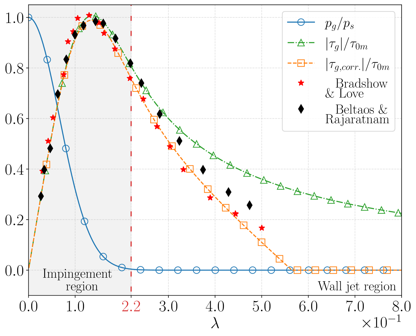
Figure 3 shows the normalised pressure (solid blue line with circles) and shear stress (orange dashed line with squares) distributions, compared to the shear stress distribution proposed by Beltaos and Rajaratnam [40] (dash-dotted line with triangles) and the shear stress measurements from Beltaos and Rajaratnam [40] (black diamonds) and Bradshaw and Love [42] (red stars). The stress distributions are more pronounced in the impingement region (grey area) (), and gradually decrease to zero in the wall jet region (). Our modified shear stress distribution, given by (30b), more accurately predicts the experimental data than Bradshaw’s correlation, which deviates from observed values outside the impingement region.
IV.2 Modelling electromagnetic actuators
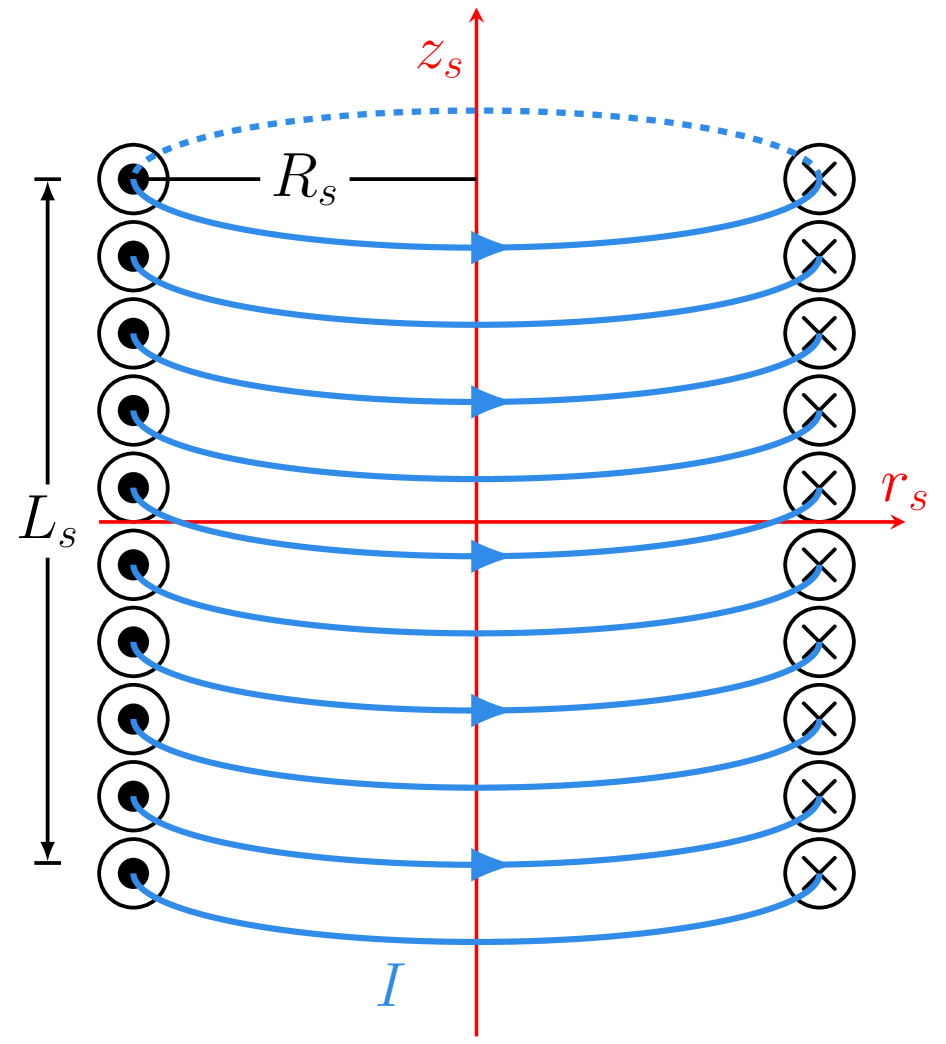
The electromagnetic actuators are modelled as cylindrical solenoids perpendicular to the substrate with length , radius , and metal core with magnetic permeability . Figure 4 shows a solenoid schematic containing coils and carrying a time-varying current . In a cylindrical reference frame centred at the midpoint of the solenoid, the magnetic field is given by complex analytical expressions derived by Hampton et al. [43] (see Appendix B for more details).
Assuming that the liquid film is positioned at a distance and considering a region near the centerline (), the radial component of the magnetic field can be neglected and its axial component ( in the reference frame of the liquid film) can be approximated as a 2D Gaussian in the plane, with a time-dependent modulation described by the control function . The approximated magnetic field reads:
| (31) |
where () denotes the position of the Gaussian’s centerline and is the nondimensional standard deviation. The dimensional value of defines the spatial scale at which the electromagnet affects the liquid film (). This value is important for calculating the characteristic timescale of the magnetic effect according to (12).
The maximum frequency of is constrained to avoid modeling the skin effect. This effect consists in an increase of the liquid film’s electrical resistivity due to electric currents concentrating in a thin region near the free surface referred to as the skin thickness , reading [44, Section 11.4]:
| (32) |
This thickness represents the depth within the liquid film at which the amplitude of an electromagnetic wave decreases to (approximately 37%) of its initial value at the surface. To ensure that the skin effect can be neglected, we require that remains larger than the liquid film thickness , leading to an upper bound on for , given by:
| (33) |
To minimize the error between the approximated form (31) and the analytical solution [43], we derived a relation between the nondimensional amplitude , the standard deviations , and the geometrical and physical characteristics of the solenoid (detailed in Appendix B), which read:
| (34) |
These relations can help design an experimental setup: given the shape and intensity of the magnetic field used in our simulations, they allow for defining the electromagnet geometry, the number of coils, and the time-dependent current profile in the experimental setup.
V Numerical Methods
The IBL model in (22) was implemented in numerical software using the Fourier pseudo-spectral method for spatial discretization [45, 46]. This method transforms the physical quantities from a physical space to a Fourier wave number space, where the spatial derivatives are calculated analytically. The liquid film height and the flow rates and are approximated as linear combinations of 2D plane waves, where , expressed as:
| (35a) | ||||
| (35b) | ||||
| (35c) | ||||
where and are the nondimensional streamwise and spanwise wave numbers, and , , and are the Fourier coefficients.
Substituting (35) into (22), calculating the spatial derivative by differentiating (35) and subtracting the right-hand-side from the left-hand-side results gives the residual of the spectral approximation. This is then projected onto a basis of Dirac delta functions , defined on an equispaced grid (known as collocation points) where and , with such that and . Using the properties of the Dirac delta function, the inner product with the residual yields a discrete inverse Fourier transform (IDFT), which provides the values of the state variables at the grid points:
Given the values of , , and at the grid points for a specific time , the nonlinear terms are first computed in physical space and then transformed into Fourier wave number space using the Fast Fourier Transform (FFT). A 2D Finite Impulse Response (FIR) filter is applied to reduce aliasing errors, with a normalized cutoff wave number set to times the Nyquist frequency in both spatial directions. The filter is designed using a Hamming window, with the number of filter coefficients set to half the length of the input signal in each direction. The 2D filter is obtained by independently applying the dot product of the 1D filters along the and directions. Finally, the derivatives are transformed back into physical space using the Inverse Discrete Fourier Transform (IDFT), and time integration is carried out using Euler’s method.
VI Reinforcement Learning Control
The undulation control problem consists in finding the optimal weights of a parameterized feedback control law , which minimizes an objective functional accounting for the amplitude of undulation waves. Based on observations of the liquid film thickness sampled at time , the parametric feedback control law gives the value of control actions , which corresponds to the nozzle exit velocities or magnetic field intensities of the actuators. The objective functional to minimize is given by the time integral of a reward function over a liquid film simulation that lasts for a duration . In this setting, the undulation control problem is expressed as:
| (36) |
The reward function provides an instantaneous performance measure of the feedback control law and it is defined as the space integral of a running cost , over the reward region , reading:
| (37) |
The running cost function quantifies the deviation of the liquid film thickness from its initial flat state and is defined as:
| (38) |
where represents the initial thickness of the flat film at , exp denotes the exponential function and std denotes the standard deviation computation in both space and time.
VI.1 Proximal Policy Optimization
The undulation control problem (36) with (37) and (38), constrained by the 3D IBL equations (22), is solved using the Proximal Policy Optimization (PPO) reinforcement learning algorithm [27] using the implementation provided by the Stable Baselines 3 library [47].
This method uses a stochastic feedback control law, with actions sampled from a parameterized multivariate Gaussian distribution . The vectors and represent the mean and standard deviation of the distribution, and the symbol indicates the conditioning of observations . For any given set of observations , and are provided by a neural network with weights of size neurones. Using a stochastic feedback control law, variability is introduced into the action selection process, fostering the exploration of different control strategies, which ultimately enhances control performance.
The PPO seeks the optimal parametrization through a trial-and-error process, which consists of running 300 liquid film simulations in parallel, evaluating the instantaneous performance of the feedback control law, learning from the accumulated experience, and then updating its parameterization in a gradient descent fashion.
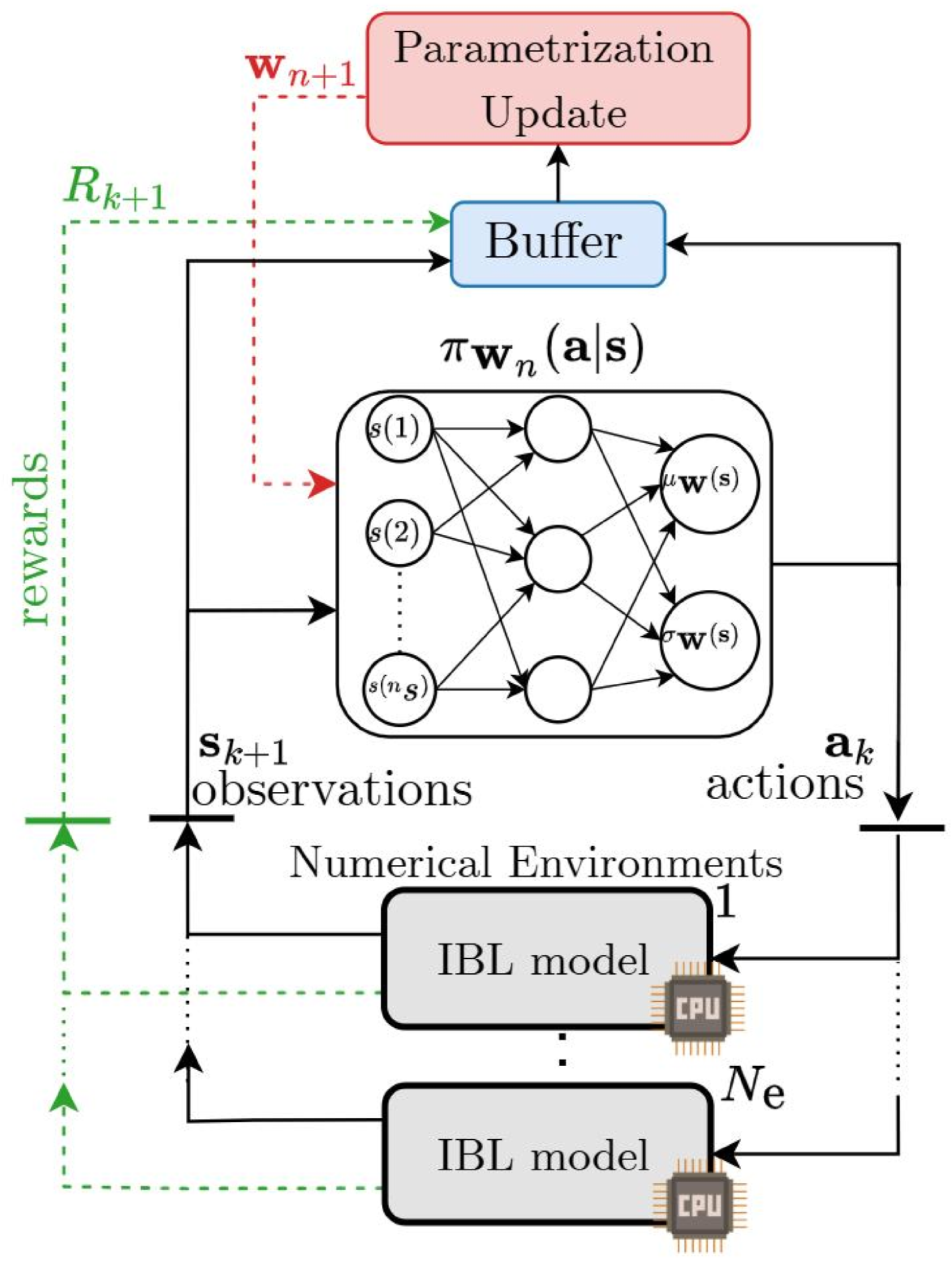
Figure 5 shows the main steps of this process: actions are sampled from the Gaussian distribution , parameterized by the neural network weights (white box). These actions are then passed on to liquid film simulations, known as numerical environments, at time , where represents the integration time step. To accelerate the optimization process, these numerical environments are executed in parallel across multiple CPUs (grey boxes), simulating shifted undulation waves to increase variability and enhance the chances of learning a better parameterization (more details are provided in Subsection VI.2).
The actions , which differ across environments, are held constant for integration time steps to prevent sudden changes that could hamper the PPO learning process. At the end of this period, each numerical environment outputs a vector of liquid film observations evaluated at the last timestep of the integration period , along with a total reward function given by the sum of the reward function at each time step, which reads:
| (39) |
The sequence of actions, observations, and rewards gathered during a simulation of duration constitutes a trajectory. The final time is defined as , where represents the algorithm’s total number of interactions with the numerical environment per simulation. Trajectories from different simulations and numerical environments are stored in a buffer (blue box).
Leveraging the knowledge of liquid film dynamics acquired from stored trajectories, the PPO algorithm enhances control performance by updating the weights every time . This update is made by maximizing a clipped objective function, which entails the minimum of the probability ratio between the updated control law and the old control law , along with a clipping function [48]. The maximization problem is formulated as:
| (40) |
where is the advantage function and denotes the empirical average over the trajectories in the buffer collected with the old control law.
The advantage function estimates the benefit of taking an action given an observation and reads:
| (41) |
where is the discount factor that determines the weight of future rewards, and represents the value function. This function calculates the expected sum of rewards starting from a given state , with actions chosen according to the control law until the last interaction with the numerical environments () and it is defined as follows:
| (42) |
The value function is approximated by a separate neural network of size neurones and is updated using the sum of the rewards collected in the buffer.
The sign of the advantage function is used to prevent the algorithm from making too large updates in (40), which could result in ineffective control laws. To this end, the clipping function defines a confidence region around the probability ratio , based on the sign of , ensuring that successive control laws do not differ too much from one another. This function is defined as:
| (43) |
where is a hyperparameter that defines the clipping range.
VI.2 Control test cases
This section describes the numerical environment used to solve the control problem introduced in Section VI using the PPO algorithm presented in Subsection.
The IBL equations are discretised in space using the Fourier pseudo-spectral method (Subsection V) over a uniform grid of points along and along . The discrete system is integrated in time via the explicit Euler method with a time step ().
We consider an initially flat liquid film, with thickness and flow rates given by:
| (44) |
The computational domain is a rectangle of size in the streamwise direction and in the spanwise direction. Figure 6 shows a schematic of the numerical environment where the domain includes a set of control gas jets (red crosses) and electromagnets (green squares), the locations of the observation point of the liquid film thickness (indicated by red dots), a series of forcing jets aligned along the direction (depicted by blue circles) and a Perfectly Matched Layer (PML) (light green area) around the periodic boundaries (black contour line).
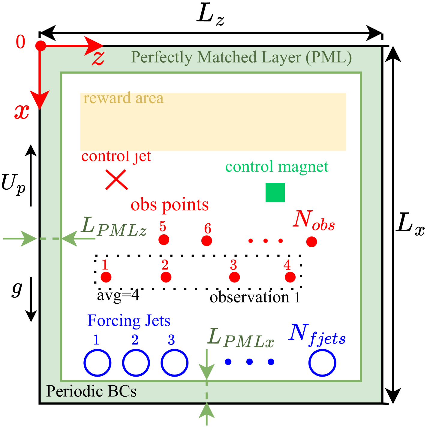
The PML is used to simulate open-flow conditions. This layer absorbs the incoming waves without reflection, preventing them from re-entering the domain through the periodic boundaries. A linear perfectly matched layer [49, 50] is implemented with dimension and . The PML is implemented by replacing the spatial derivative with the following expressions:
| (45) |
where is the angular frequency of the liquid film waves and and are positive functions which determine the strength of the absorbing layer, defined as:
| (46a) | |||
| (46b) |
The transformation in equation (45) involves introducing a set of auxiliary equations, discretized both in space and time, similar to the IBL equations. For convenience, these equations are provided in Appendix C.
Moving to the undulation instability, this appears in the liquid film as two-dimensional waves propagating streamwise, with minimal variations along . Numerical simulations from Large Eddies Simulations (LES) [51] and 2D IBL model [17] indicate that these waves are characterized by a nondimensional frequency in the range , a peak-to-peak amplitude ranging from to of the unperturbed film thickness, and wavelengths within the range .
To reproduce these characteristics, we use a set of blowing and sucking gas jets. The nozzle exit velocity of these jets varies with a harmonic function of the nondimensional time , with a random phase shift to induce a small variation in the spanwise direction. The exit velocity of the -th forcing jets reads:
| (47) |
To introduce greater variability into the simulation and promote the learning of robust control functions, the amplitude and the frequency are modelled as finite Fourier series with randomly selected coefficients and [52], reading:
| (48) |
where the coefficients and , which are different for the amplitude and the frequency, are sampled from the normal distribution . Based on (48), the amplitude and frequency are rescaled in the range of interest as:
| (49a) | |||
| (49b) |
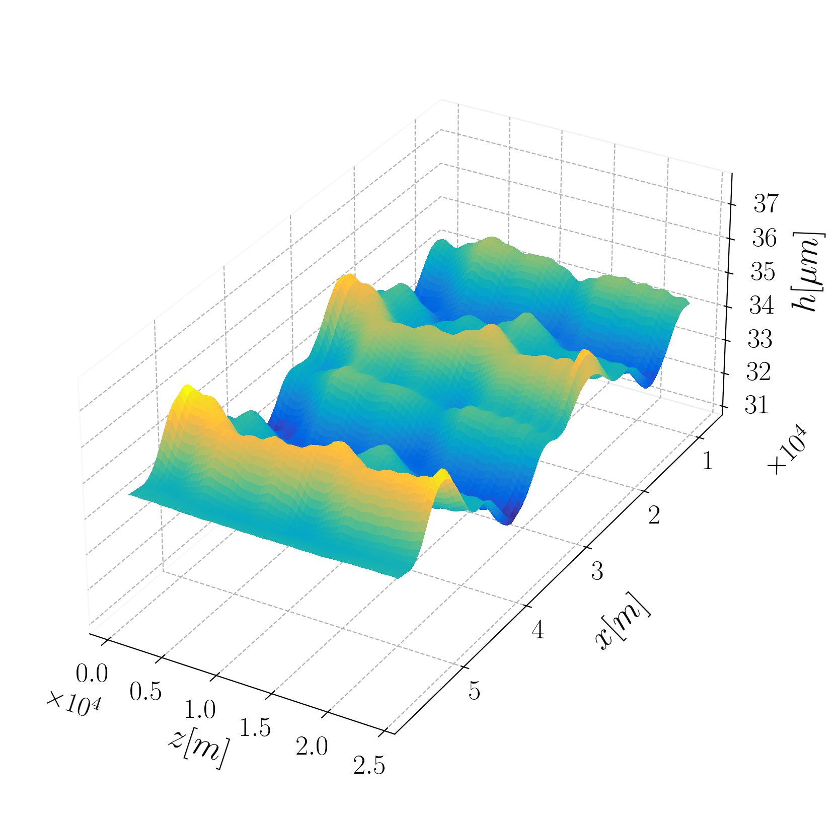
Figure 7 shows the nondimensional uncontrolled liquid film with the undulation instability induced by the forcing jets propagating through the domain. The wavelength ranges from to , in the range of most amplified waves identified inMendez et al. [17].

Regarding the control actuators, as introduced in subsection IV, the magnetic field , is approximated as a Gaussian function centred at with standard deviation where , and is the control parameter. Although the standard deviation and the Hartmann number (), do not lie on the Pareto front of optimal solutions [3], the magnetic Gaussian roughly spans half the wavelength of the undulation instability, allowing the controller to direct the electromagnet’s action to either a valley or a crest.
The pressure and shear distributions of the control and forcing jets are modelled using experimental correlations for 3D impinging circular jets (see Subsection IV), with the velocity at the jet nozzle exit, , used as the control parameter. To avoid sharp changes in the control action, this is smoothed with an exponential moving average, reading:
| (50) |
where is the action passed to the solver, is the action selected by the PPO and is the action passed to the solver at the previous interaction with the film.
Three distinct actuator configurations were analysed: a standalone 2D gas jet, a standalone 2D electromagnet, and a combination of both actuators. A harmonic control action was applied with amplitude, frequency, and phase variations throughout the simulation in the standalone configurations.
Figure 8 illustrates the numbering and placement of the three liquid film observations (red dashed lines) and the actuators (black dashed and dash-dotted lines) for the case with a single (left) and double (rights) actuators.
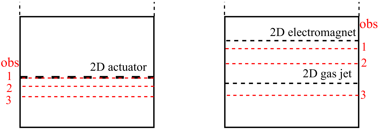
The three liquid film observations are the average liquid film thickness sampled at four points along at three locations along . For a single 2D actuator, these are placed at and . For the two 2D actuators, these are placed at and .
Concerning the reward area (yellow area in Figure 7), in the case of a single actuator, this is defined as and in the case of two actuators
VII Results
This section is divided into three subsections. Subsection VII.1 reports on the asymptotic behaviour of the steady-state solution and the closure terms for a magnetic field approaching zero. Subsection VII.2 reports on the wave dynamics that arises when setting the non-linear phase speed in the leading order in the IBL model. Finally, subsection VII.3 reports on the results of Reinforcement Learning control of the unstable undulation perturbations using gas jets and electromagnetic actuators, considering both standalone and tandem configurations.
VII.1 Asymptotic Behaviour
In this subsection, we analyse the behaviour of the steady-state solution found in Subsection III.2 and the closure relations introduced in Subsection III.4 as the magnetic field and the Hartmann number Ha approach zero.
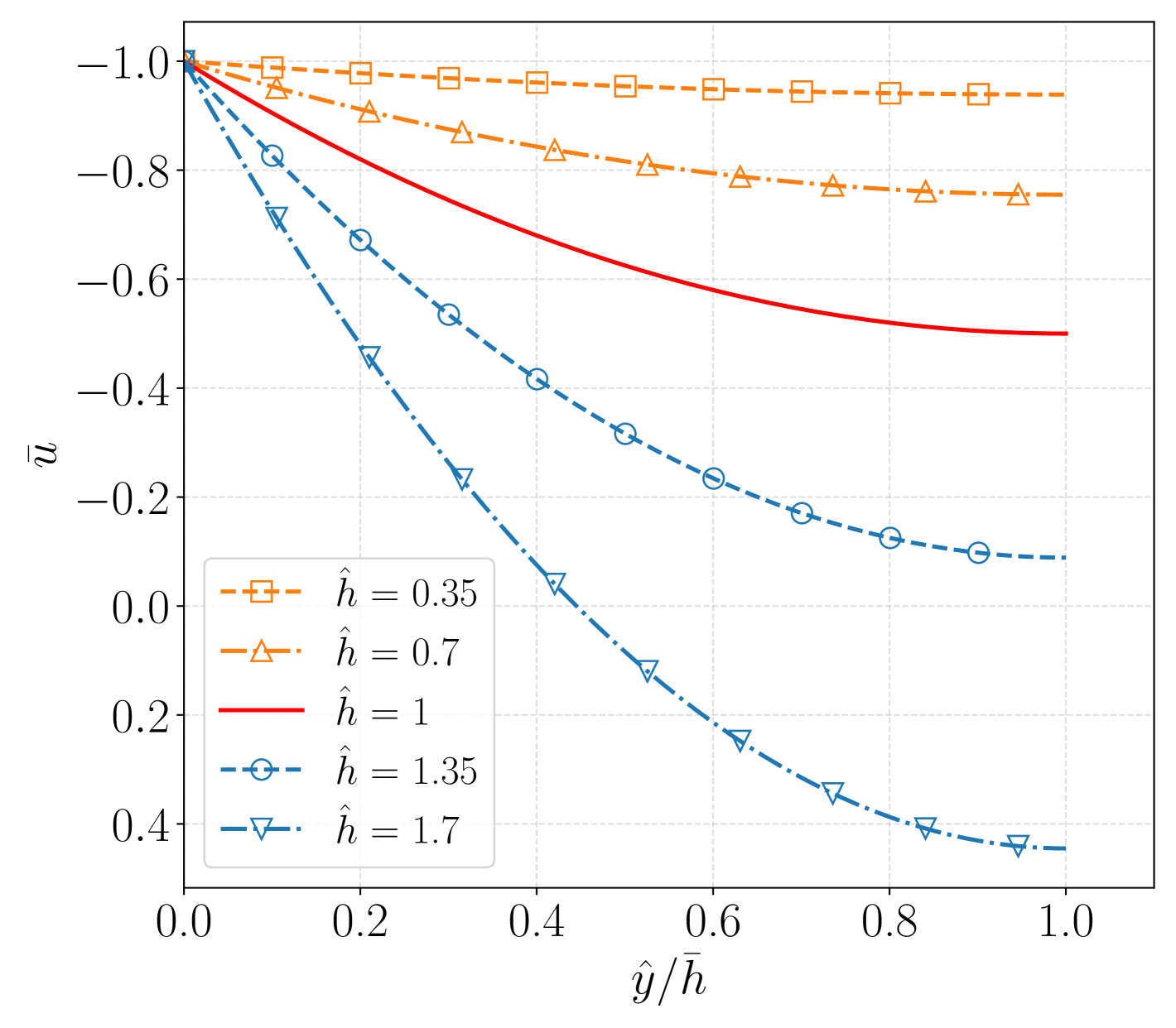
Expanding the steady state velocity profile (17) in Taylor series around () gives:
| (51) |
The velocity reaches a well-defined limiting value, as it recovers, at leading order, the solution that was previously derived in the case without magnetic field by Ivanova et al. [34]. This result serves as the first analytical validation of our model, confirming its asymptotic consistency.
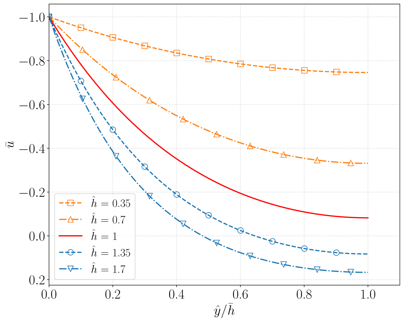
Figure 9 presents the steady-state results for case (a) without and (b) with a magnetic field (), for different values of . In both cases, the velocity profile is parabolic, but the variation between the different profiles is more pronounced in the absence of the magnetic field. In particular, the magnetic field has a more significant effect when , where the streamwise velocity remains negative, balancing the gravitational effects. In contrast, without the magnetic field, the downward gravitation force causes the velocity to become positive for most of the liquid film thickness.
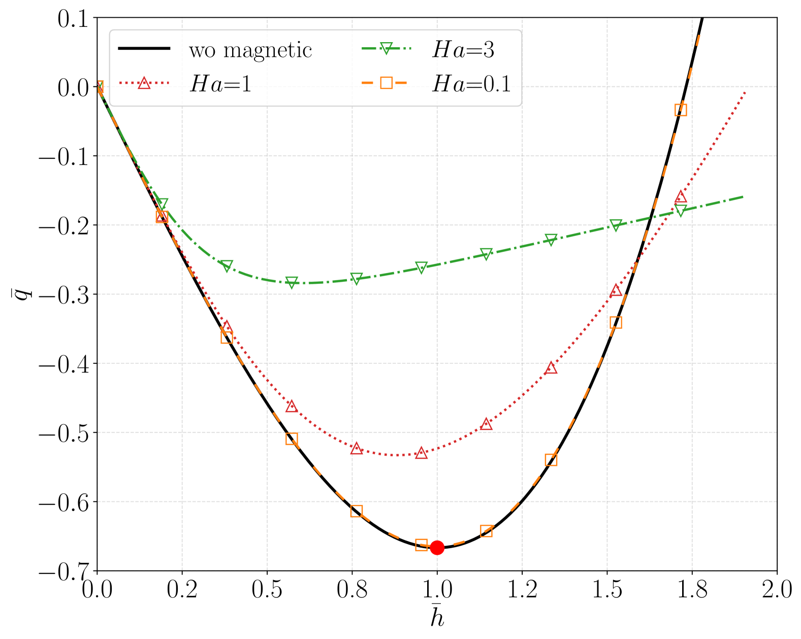
Moving to the steady-state flow rate (18), Figure 10 shows the relationship between and for different values of Ha (lines with markers) and the case without a magnetic field (black continuous line). Like the velocity profile, recovers the case without a magnetic field as . In the absence of the magnetic field, has two solution branches: thin film () and thick film (), with a minimum at , corresponding to the flat film solution of Derjaguin [53]. The branch with in the range is attainable solely by withdrawing the substrate from the bath and, at the same time, feeding the liquid film from above.
When the magnetic field is applied, the minimum moves towards smaller flow rates and thinner film thicknesses as Ha increases. In addition, the position of the zero net flow rate changes to higher values of as Ha increases. This indicates that the locus of possible steady-state solutions, attainable by simply extracting the liquid film from a bath, expands with the application of the magnetic field.
The same asymptotic behaviour observed for the steady-state velocity profile in (51) also applies to the flux terms and the wall shear stress closure relations. The Taylor expansions of (27) and (28) around the point () are as follows:
| (52a) | ||||
| (52b) | ||||
| (52c) | ||||
| (52d) | ||||
| (52e) | ||||
The closure relation exhibits a regular limit, recovering at leading order the values obtained in the absence of the magnetic field found by [34]. This provides an additional analytical validation of our model, showcasing the consistency of the term entering the unsteady equations.
VII.2 Leading-Oder convective velocity
Having established the consistency of the IBL model with the non-magnetic case under both steady and unsteady conditions, this section investigates the effect of magnetic forces on the phase speed of surface waves. To this end, we neglect all terms of order in (22), assuming the pressure gradient terms of order , and everywhere in the domain. Under these assumptions, the solution to (22) is given by the steady-state solution (18) for the flow rate, with zero flow rate along the -axis. Substituting this into the integral form of the continuity equation yields a convection equation for the liquid film thickness, which is given by:
| (53) |
where is the nonlinear phase speed, reading:
| (54) |
The Taylor expansion of (54) around , reads:
| (55) |
As for the cases treated in subsection VII.1, the leading-order term is consistent with the case without magnetic field [34].
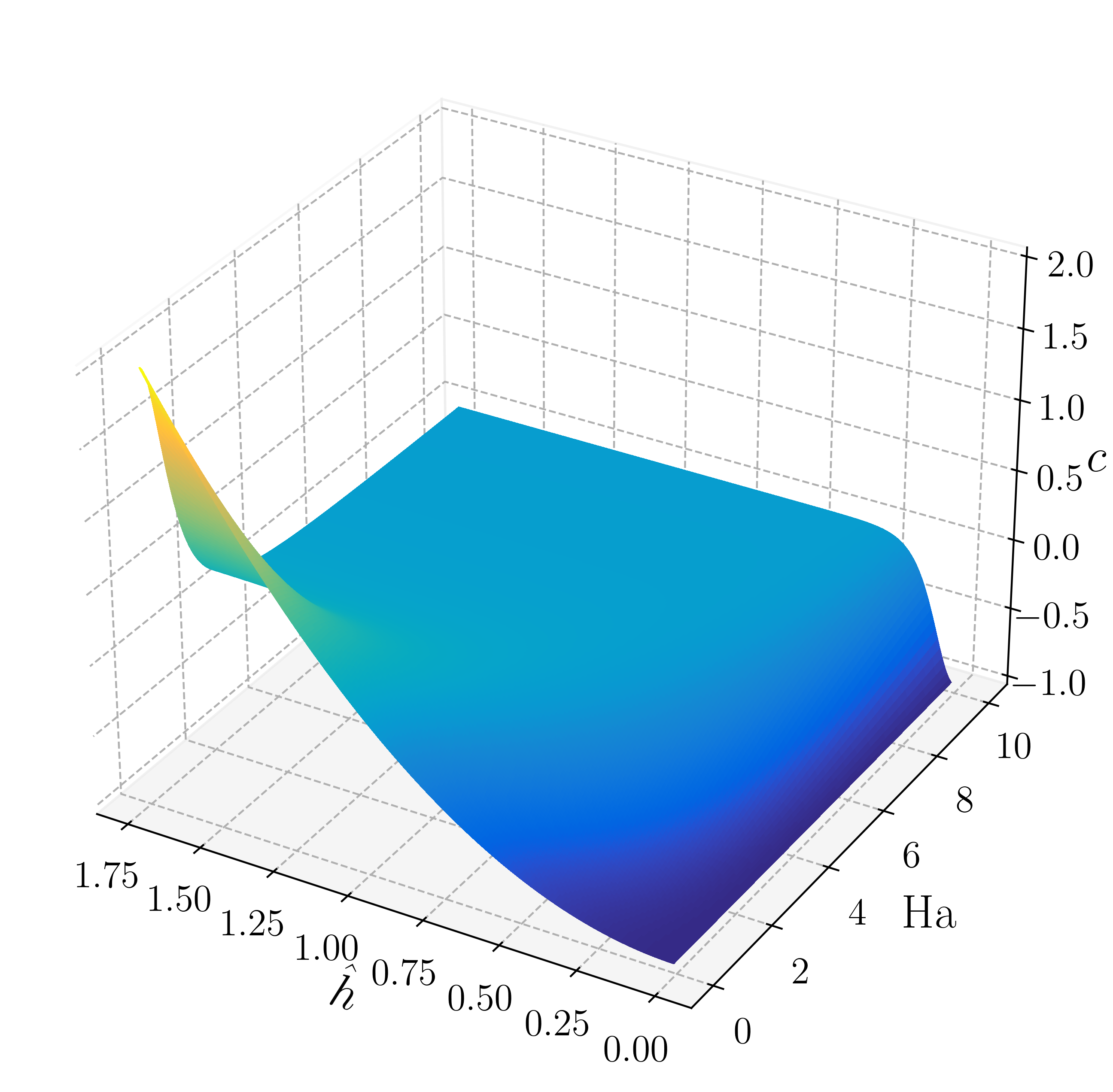
Figure 11 illustrates the phase speed (54) as a function of the non-dimensional thickness and the Hartmann number Ha. For small values of Ha, has a quadratic dependence on , with waves propagating upstream () for and downstream () for . For , reaches a plateau at approximately for . As we have already seen in figure 9(b), the magnetic effects for these conditions counterbalance the gravitational effects, resulting in an equilibrium solution where waves always propagate in the direction of substrate movement. This highlights how the magnetic force might affect the absolute/convective instability properties of these flat film solutions compared to the case without a magnetic field [54].
VII.3 Undulation control using Reinforcement Learning
In this section, we present the results of the undulation control problem outlined in subsection VI.2, using the PPO algorithm introduced in subsection VI.1. We examine the cases with a single gas jet or electromagnetic actuators and the cases where these are used together. The results are presented in terms of learning curves, the mean, and standard deviation over the testing episodes, the evolution of the control function over time, and snapshots of the liquid film along the centreline.
VII.3.1 Control with 2D gas-jets
The first case involves a single 2D gas jet actuator in the case of a prescribed harmonic control function and in the case where the agent is free to take any action in time.
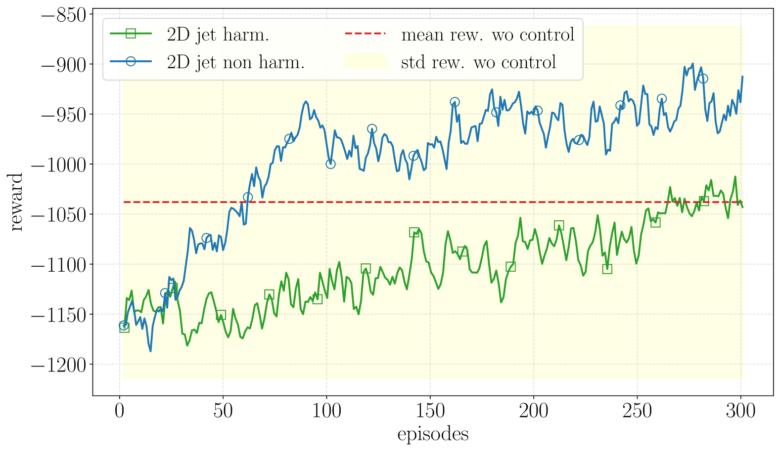
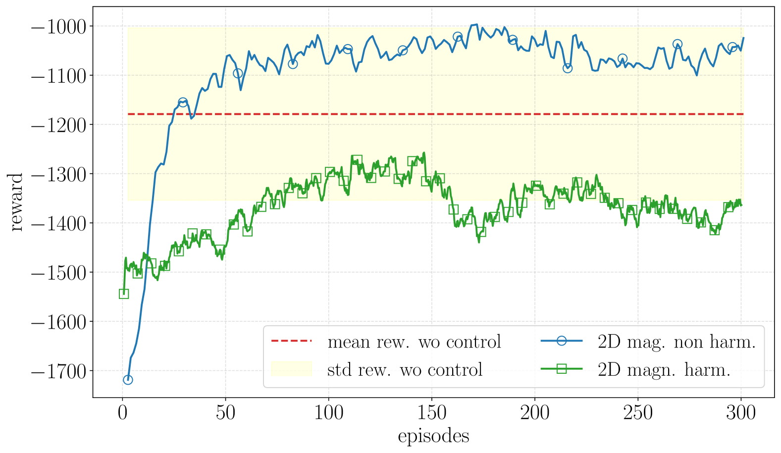
Figure 12 shows the learning curves for the case with a single 2D gas jet, comparing the harmonic control function (green curve with squares) and the nonharmonic control function (blue curve with circles) against the mean (red dashed line) and the standard deviation (yellow shaded area) of the uncontrolled case. Both control functions achieve mean rewards at the end of the training that exceed those of the uncontrolled case.
| Reward | wo Control | Harmonic | Non-harmonic | ||
|---|---|---|---|---|---|
|
-1038 | -826 | -790 | ||
|
176 | 153 | 136 |
Table 2 summarises the mean and standard deviation of the evaluation episodes for controlled and uncontrolled cases. Like in the learning phase, both control functions result in a higher mean reward than in the uncontrolled case. Furthermore, in the controlled case, the reward variability around the mean is reduced, with a smaller standard deviation. This shows how the PPO managed to find an effective control action that led to a reduced undulation amplitude in the reward area.
Focussing on the harmonic case, the evolution of the optimal control function during an evaluation episode is reported in figure 13. Figure 13(a) shows the amplitude (solid red line with squares), the nondimensional frequency (blue dashed line with triangles), and the phase shift (dotted dashed line with circles) of the harmonic control function during an evaluation episode. These three parameters remain nearly constant, with an amplitude of , a frequency of , and a phase shift of . The frequency aligns with the average frequency of the undulation waves, which ranges between and . This shows how a single harmonic function is sufficient to reduce the amplitude of the undulation instability.
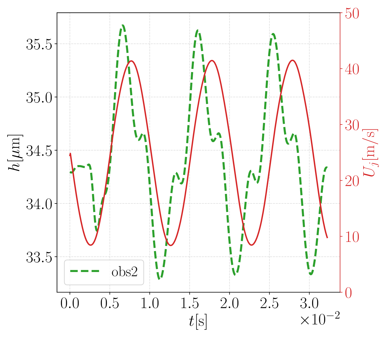
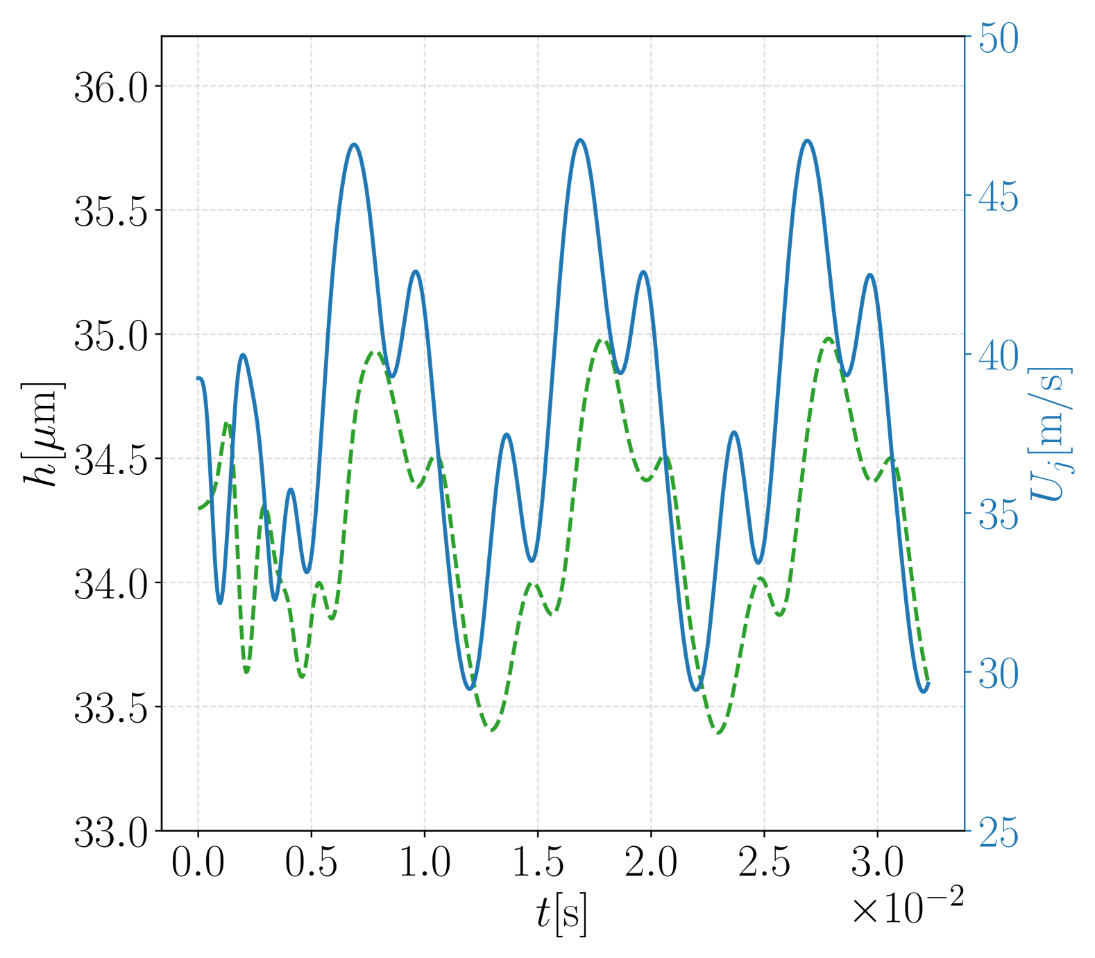
To gain a better understanding of the control mechanism, we look at the evolution of the control function compared to the observation of the liquid film collected at one of the three observation locations. Figure 13(b) shows the evolution of the nozzle exit velocity (solid red line) and the observation at obs2 (solid green line). The positions of the crests and valleys of the two functions are very similar, with only a small phase shift because the observation point is located ahead of the control actuator. This shows that the jet primarily flattens the crests with only a minor effect on the valleys. However, since the nozzle exit velocity is always non-zero, this indicates that the optimal control law involves a thinning of the liquid film and a harmonic component nearly in phase with the instability wave.
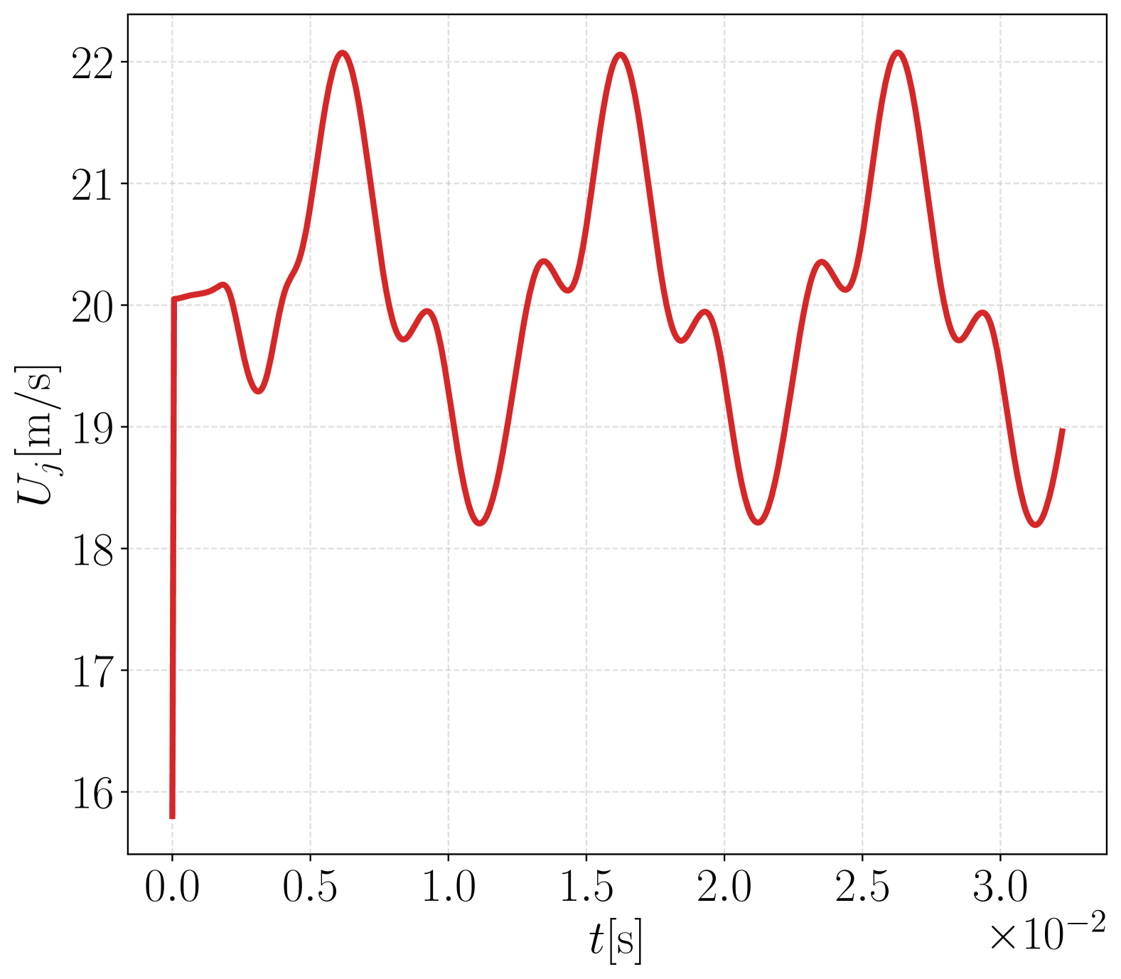
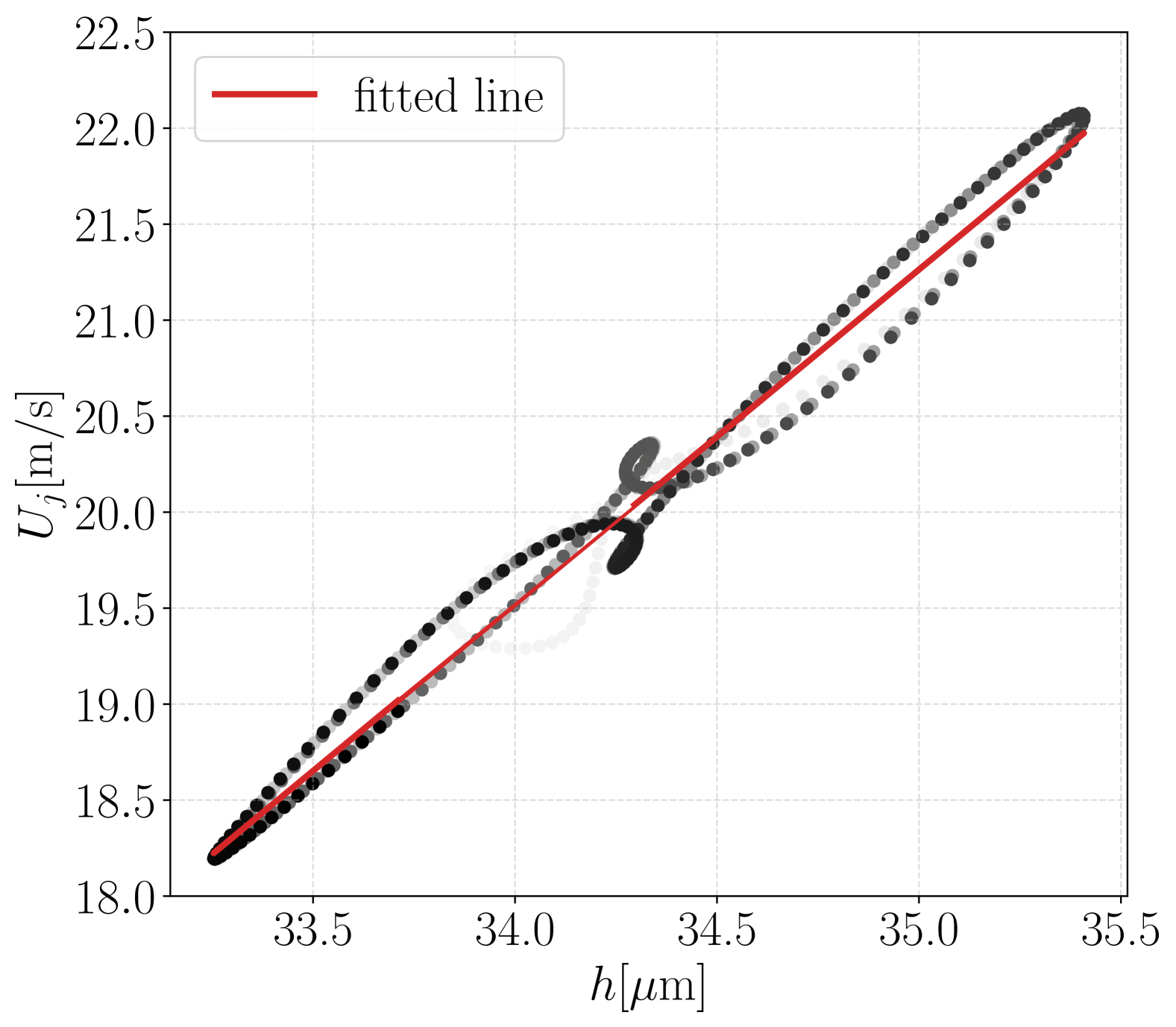
Moving to the case where the PPO is free to take any actions, figure 14 shows the evolution of (a) the control actions and the relation between the control actions and (b) the obs1 with the fitted line (red curve) for the non-harmonic control function. The control action is proportional to the mean liquid film thickness at the impingement point with a small phase shift.
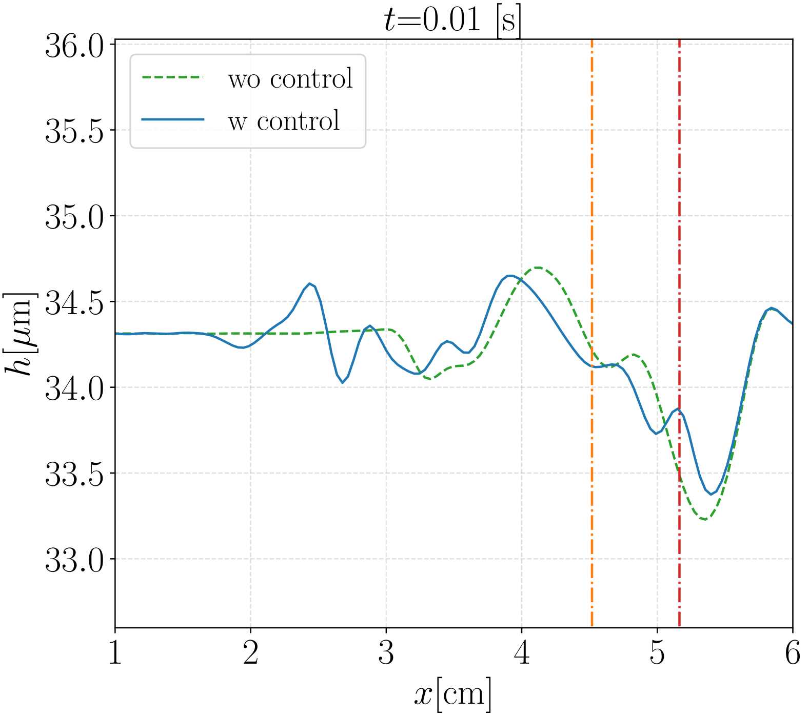
Looking at the plot along a line in the streamwise direction, figure 15 shows the evolution of the controlled three-dimensional liquid film (a, b, and c) and the comparison between the uncontrolled (green dashed line) and the controlled (continuous blue line) along at (d, e, and f). In the harmonic case, the controller reduces the amplitude of the crests with small effects on the valleys.
VII.3.2 Control with 2D electromagnets
Turning to the control with a single 2D electromagnetic actuator, Figure 16 shows the learning curve (solid black line), the mean value (red dashed line) and the standard deviation (yellow shaded area) of the reward in the absence of control. The case with a prescribed harmonic control function fails to produce good results, with the average reward well below that of the uncontrolled case, even falling outside the uncertainty region of the no-control case. This suggests that the agent could not find an efficient control law and continued to test random combinations of actions, which led to an increased amplitude of undulation within the reward area. In contrast, the agent discovered an optimal non-harmonic control law in the case without a prescribed control function shape at the 40th learning episode. This episode marks the point at which the mean reward surpassed the mean reward of the uncontrolled case. Furthermore, the mean value closely approaches the upper bound of the uncertainty region for the uncontrolled case, underscoring the robust performance achieved by the algorithm.
A similar behaviour can be observed when examining the performance during the evaluation episodes. Table 3 shows the mean and standard deviation of the liquid film with and without control, using both harmonic and non-harmonic control functions with the 2D electromagnetic actuator. The harmonic control function resulted in a mean reward that was 14% lower than the uncontrolled case, with a larger standard deviation. In contrast, the non-harmonic control function yielded a reward 8% higher than the uncontrolled case, with a smaller standard deviation.
| Reward | wo Control | Harmonic | Non-harmonic | ||
|---|---|---|---|---|---|
|
-1179 | -1345 | -1075 | ||
|
175 | 189 | 165 |
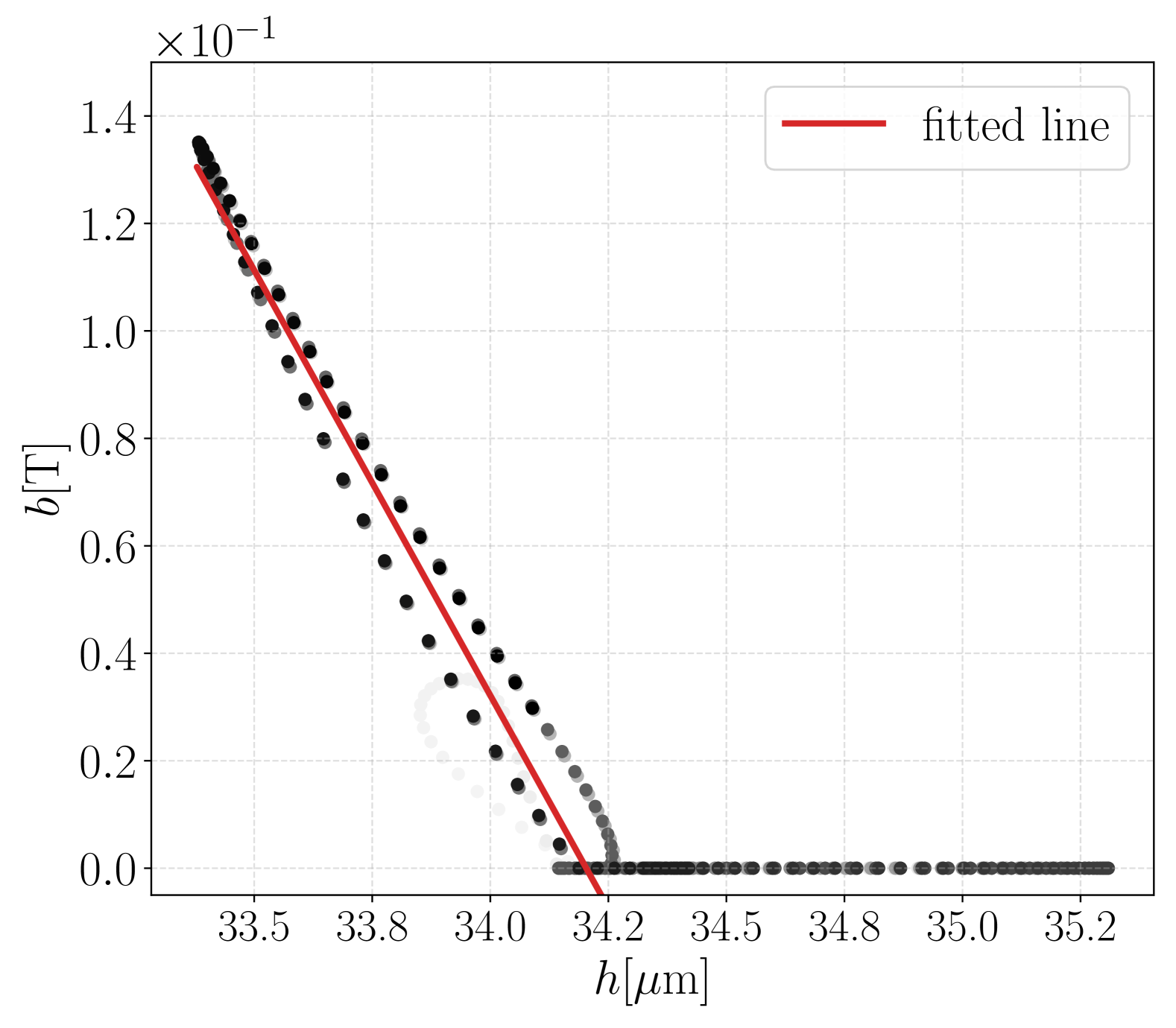
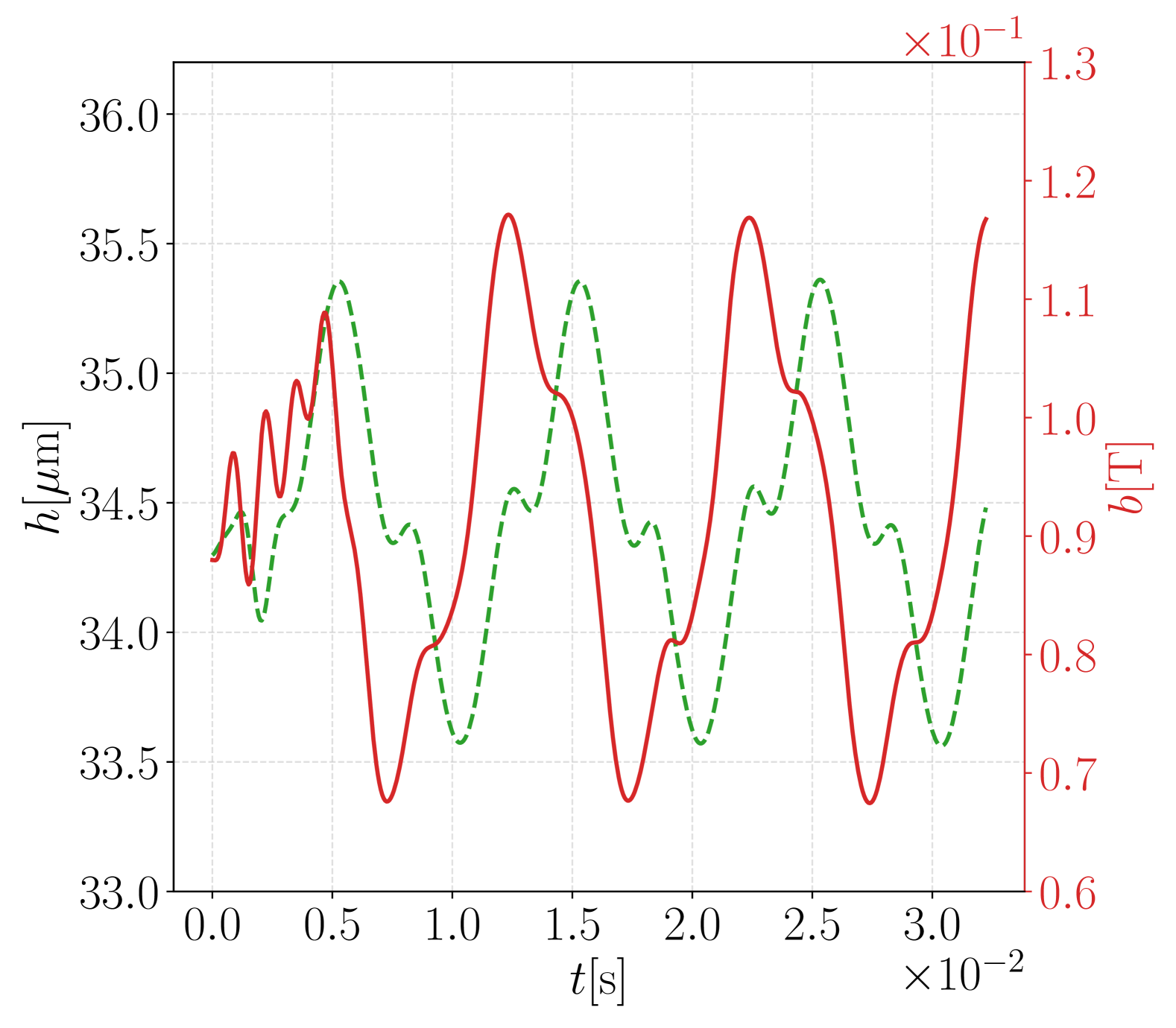
The control strategy obtained with the electromagnets differs significantly from the one we found using a single 2D gas jet. Figure 17 shows (a) the evolution of the control function (solid red line with squares) and the observations (coloured lines without markers) and (b) the relationship between the control function and obs1 during an evaluation episode. The electromagnetic control exhibits a bang-bang-type behaviour, acting only near the valleys with a maximum intensity of . The actions are inversely proportional to obs1 when they exceed the flat state of the target, .
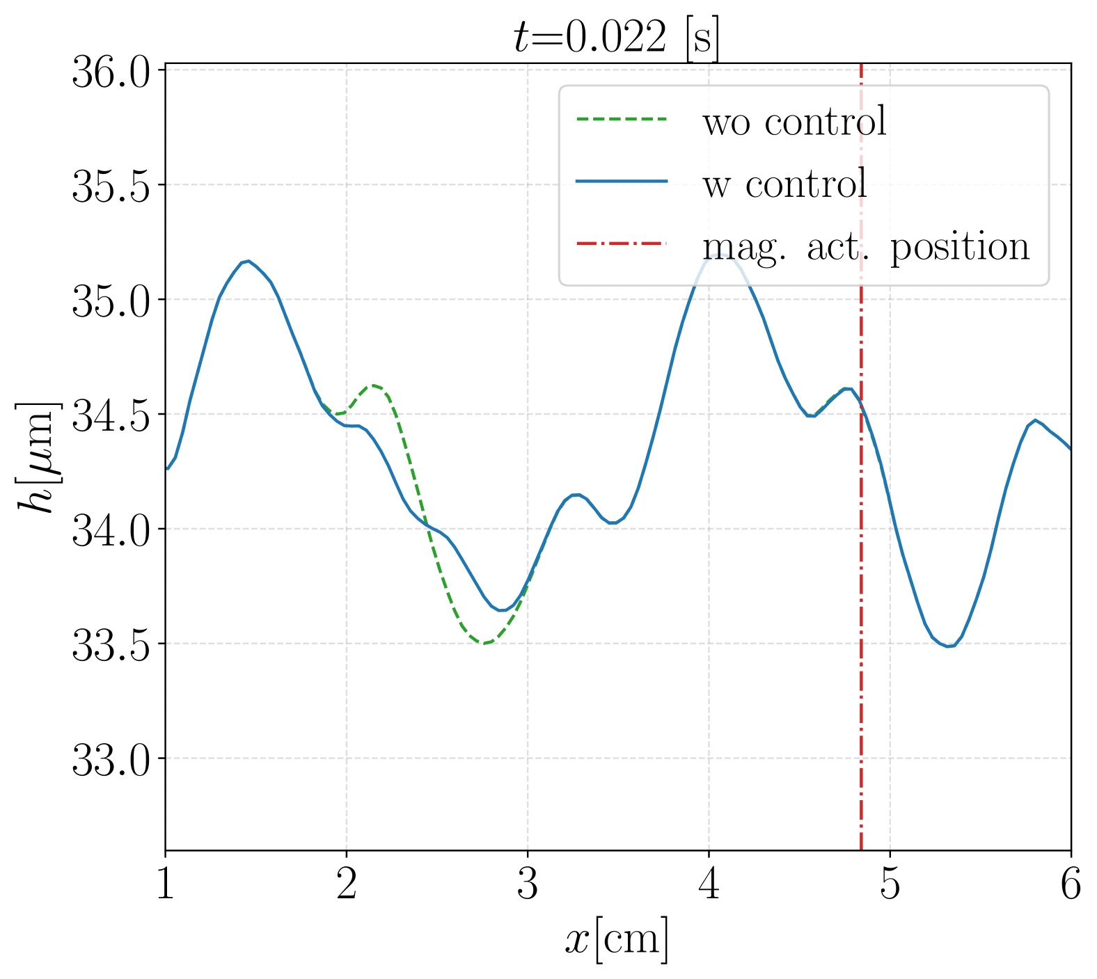
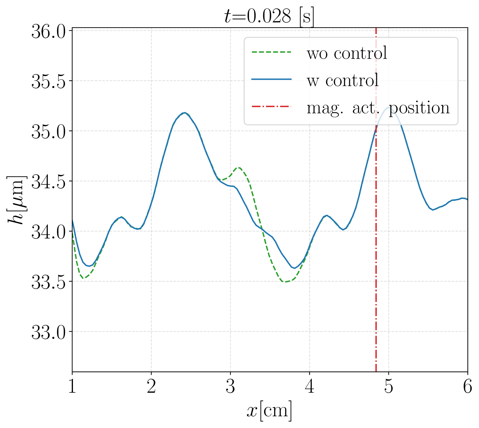
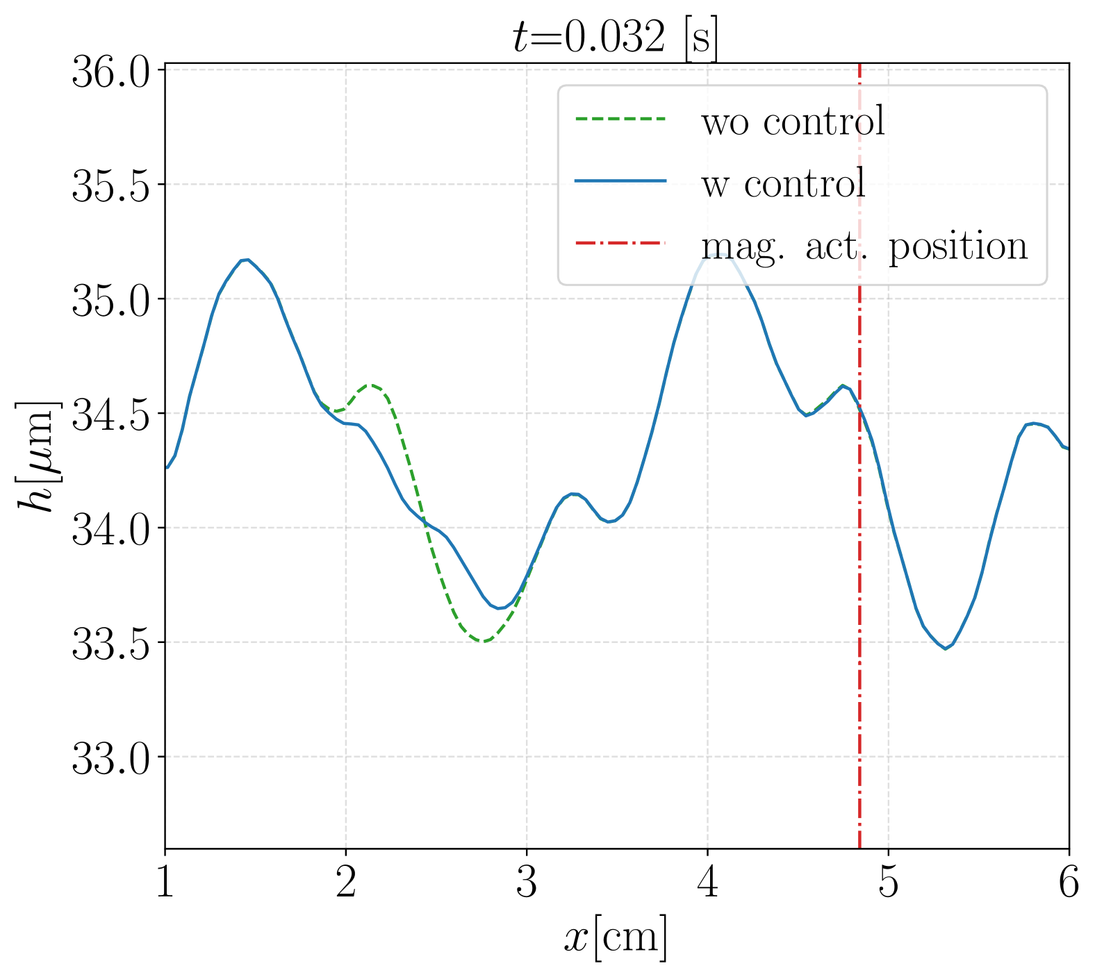
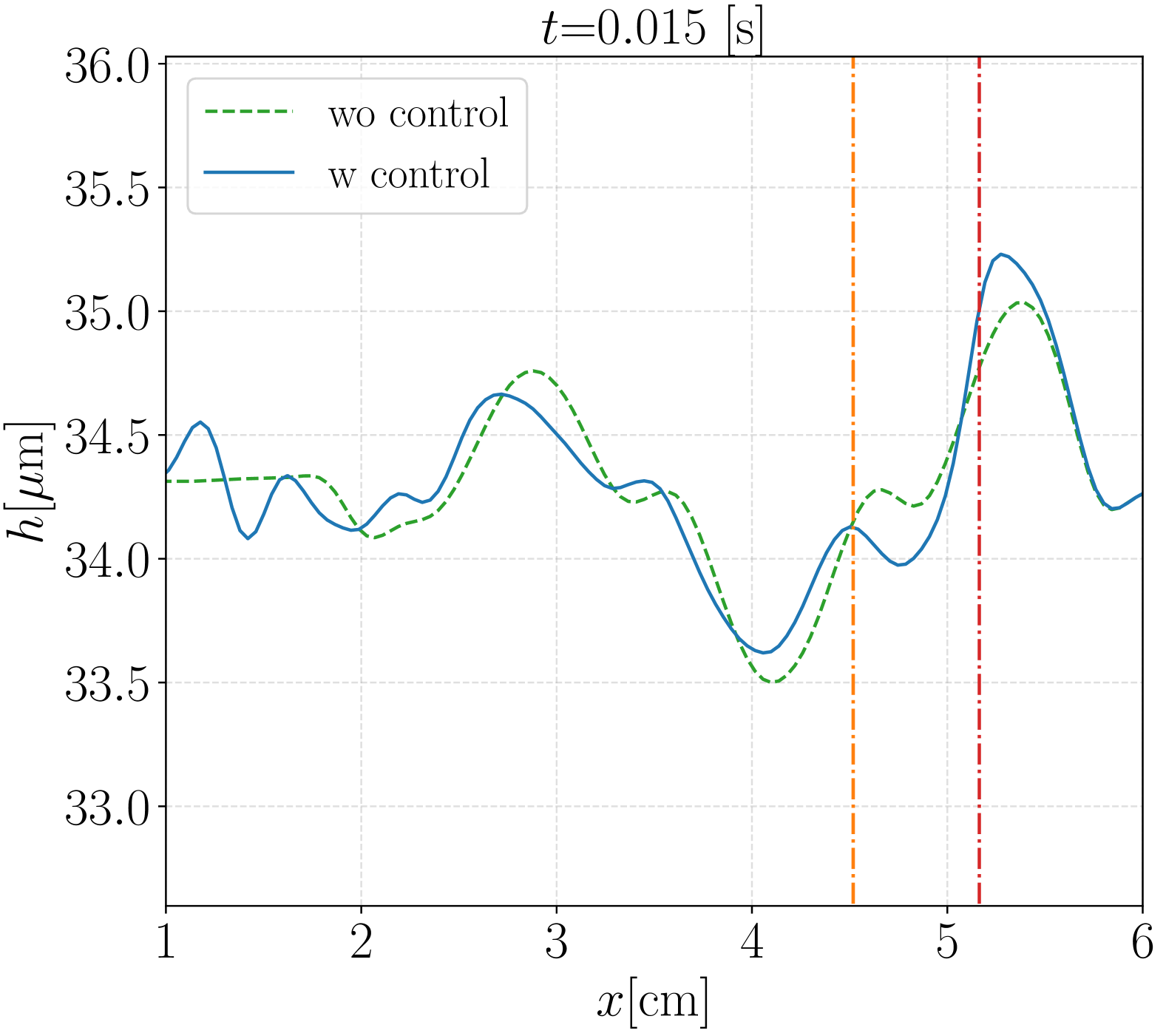
The optimal control law mechanism is due to the resistive effects of the Lorentz force on the liquid film. The Lorenz forces push the liquid in the positive direction, which creates a positive/negative flow rate gradient upstream/downstream of the electromagnet centerline. This leads to an increase/decrease in the liquid film thickness upstream and a decrease downstream. This behaviour is evident when comparing the evolution of the waves in the controlled and uncontrolled cases. Figure 18 shows the plot along for the liquid film with (solid blue line) and without (dashed green line) control. The action of the electromagnet raises and deforms the valleys, which reduces the amplitude of the nearby peaks.
This control mechanism is limited by the rapid dynamics of the liquid film, which does not provide sufficient time for the Lorentz force to flatten the free surface. As shown in Table 1, the Stuart number N, which represents the relative importance of the Lorentz force compared to inertia, is well below one (). The squared ratio between the electromagnetic and inertial time scales is given by the product of N by the film parameter as presented at the end of Section III.1. In our case, we obtain that the characteristic inertia timescale is three times smaller than the Lorentz force timescale :
| (56) |
For more efficient flattening of the liquid film, the magnetic timescale should be of the same order of magnitude as the inertial timescale, which would be possible to impose a Hartmann number given by the following relationship:
| (57) |
VII.3.3 Control with 2D gas jets and electromagnets
In the previous test cases, we found that optimal control actions of the gas jet and electromagnetic actuators complement each other. The gas jet pushes the crests, whereas the electromagnets raise the valleys. In this case, we test the control of undulations with both actuators working together. Additionally, to simplify the control problem, the agent has access to only three liquid film thickness observations instead of six.
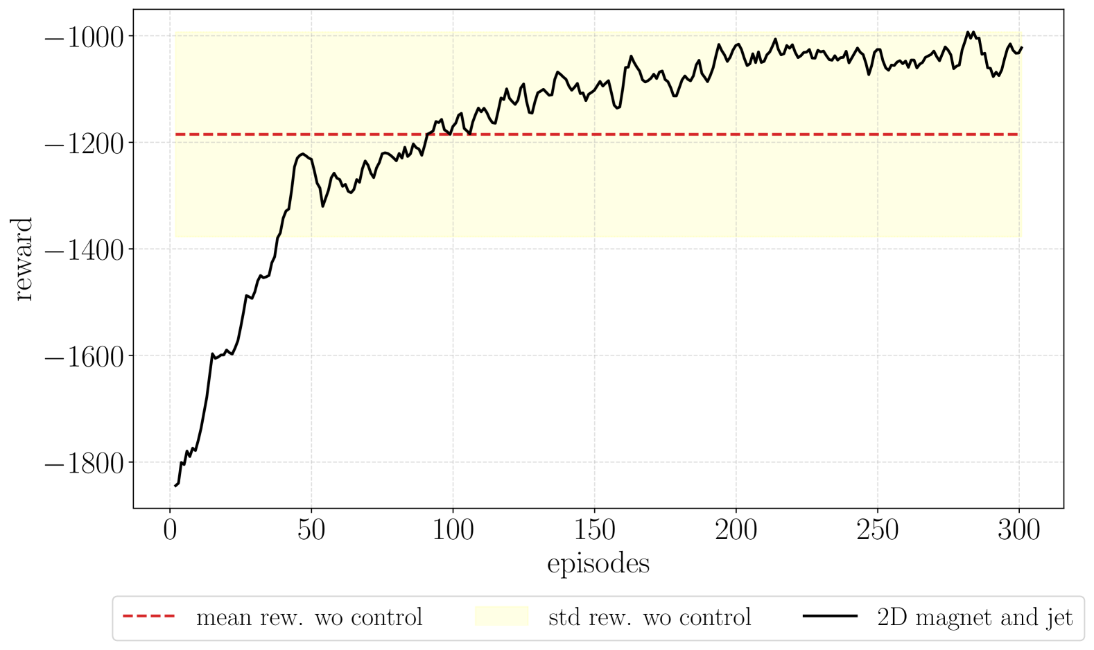
Figure 19 shows the learning curve along with the mean (red dashed line) and standard deviation (yellow shaded area) of the reward obtained without control. The PPO algorithm finds an optimal control law that outperforms the uncontrolled case after 100 training episodes. Furthermore, as observed in the case with a single electromagnet, the learning curve approaches the upper bound of the uncertainty region, demonstrating the robustness of the discovered control action. Similar results are evident in terms of evaluation episodes.
| Reward | wo Control | w Control | ||
|---|---|---|---|---|
|
-1185 | -1036 | ||
|
192 | 155 |
Table 4 shows the mean and standard deviation of the reward obtained during the evaluation episodes, both with and without control. The optimal control law yields a mean reward 13% higher than in the uncontrolled case, and a 20% reduction in the standard deviation. This indicates that even in the worst evaluation test case, the agent outperforms the uncontrolled case on average.
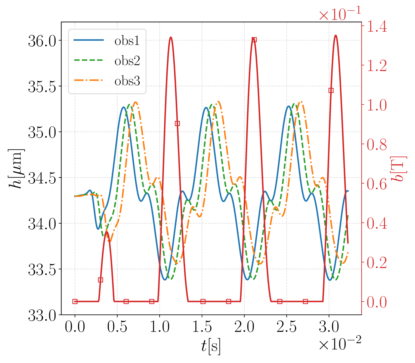
Moving to the evolution of optimal control functions during an evaluation episode, Figure 20 shows (a) the actions of the 2D gas jet (blue solid line) and obs3 (green dashed line) and (b) the actions of the 2D electromagnet (red solid line) and obs2 (green dashed line). Similarly to the case with a single gas jet, the optimal control law is nearly proportional to the liquid film observation, with a small phase shift owing to the distance between the observation point and the actuator. In contrast, the magnetic control action differs significantly from that in the standalone case. Here, the magnetic field is never zero and changes in a non-proportional way compared to the observation, unlike the gas jet’s upstream action, which alters the free surface topography and forces the electromagnet to adopt a different control strategy. Additionally, since both actuators are always nonzero, the optimal control action implies further thinning of the liquid film.
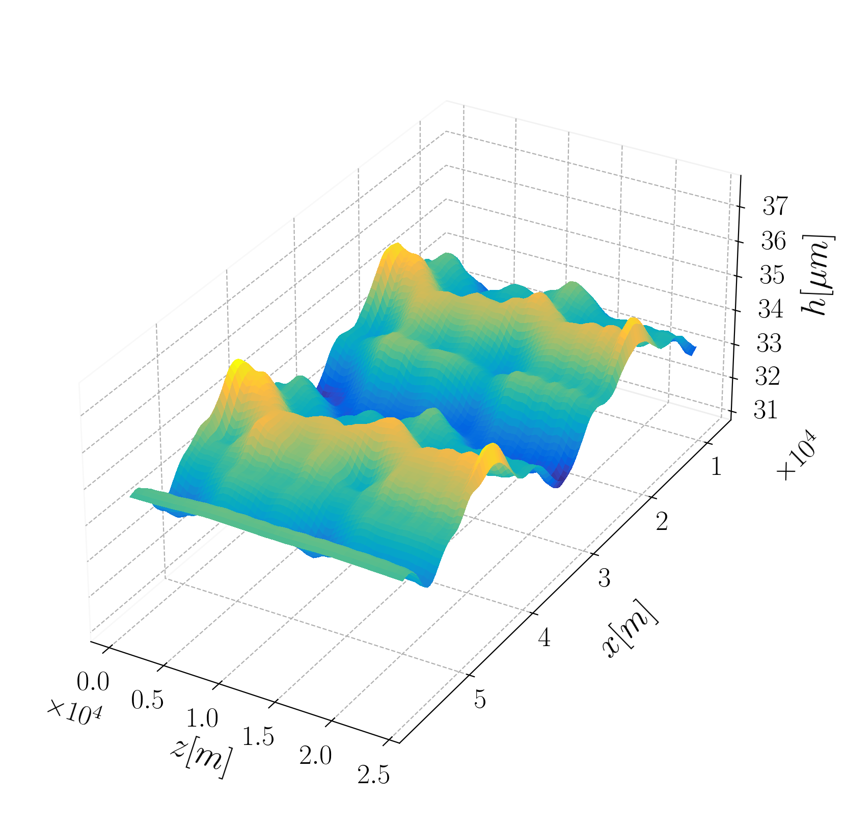
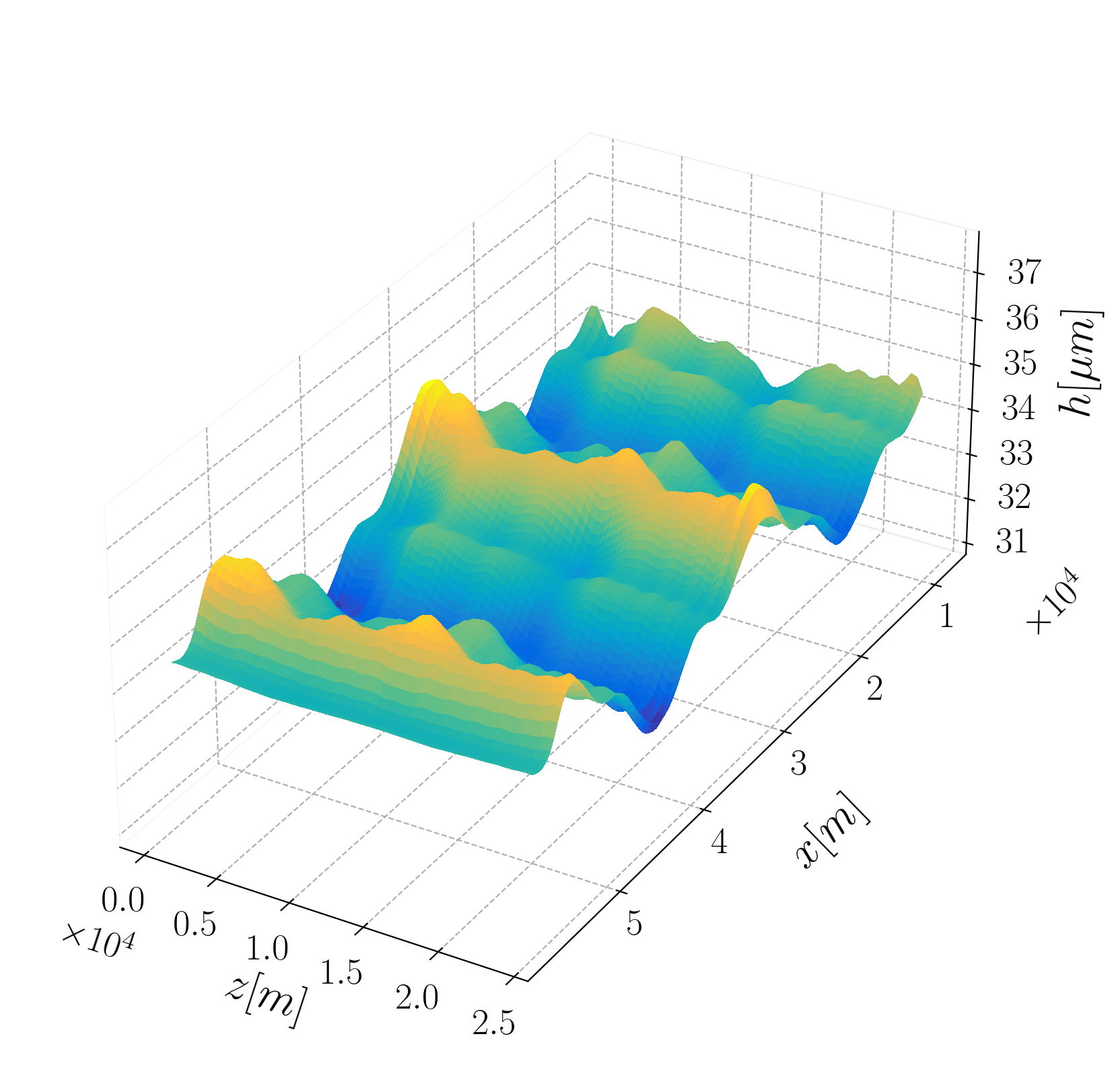
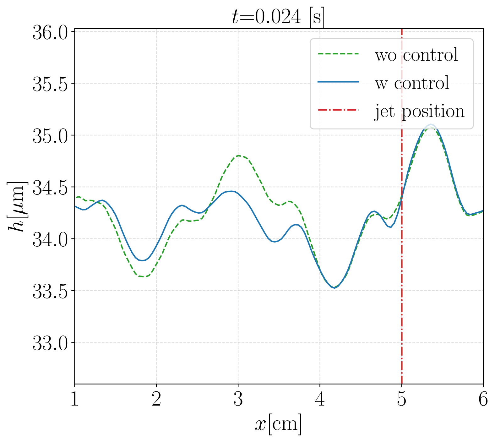
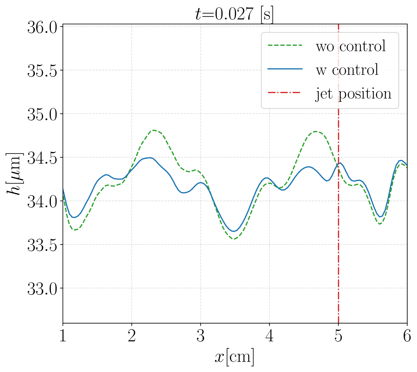
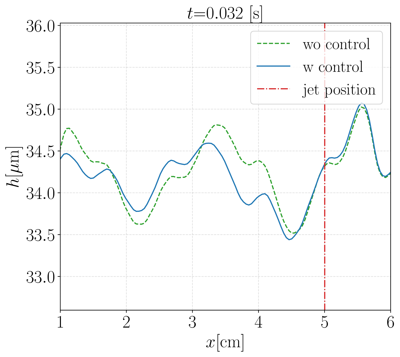
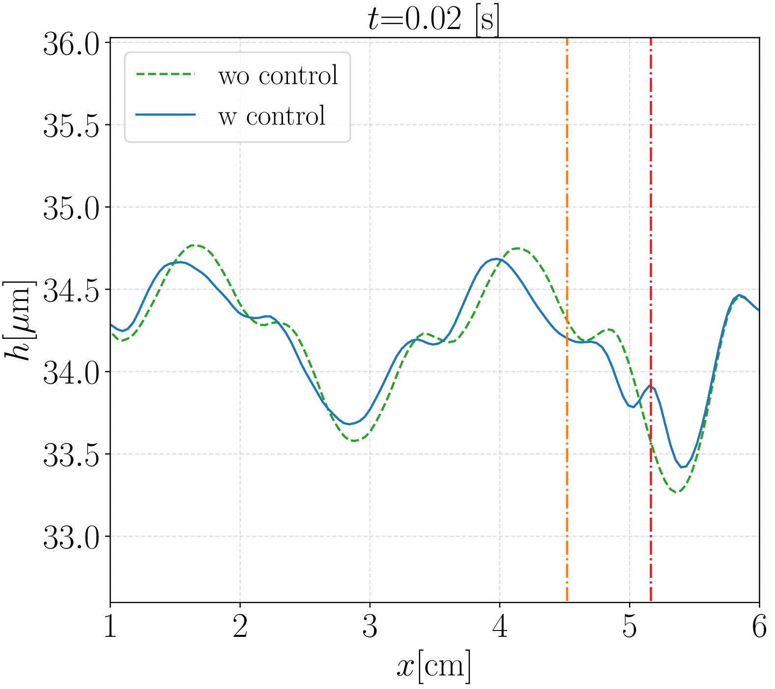
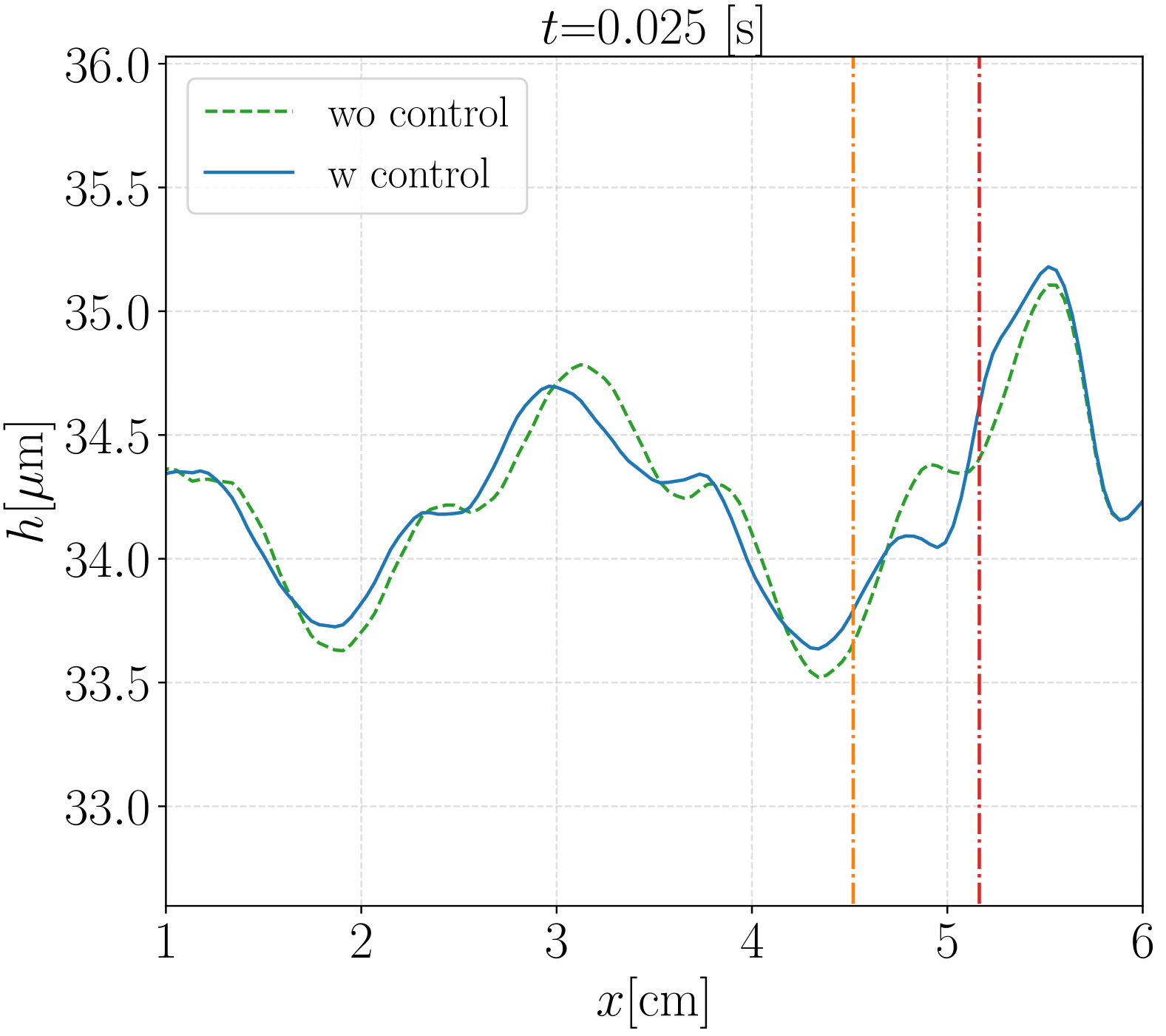
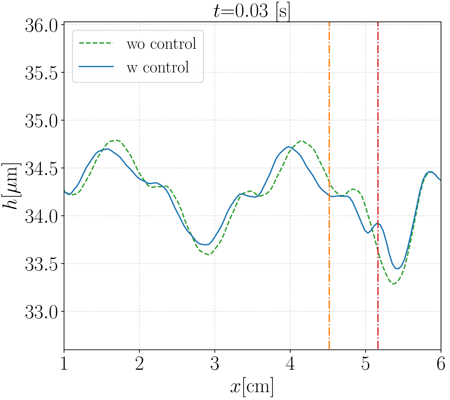
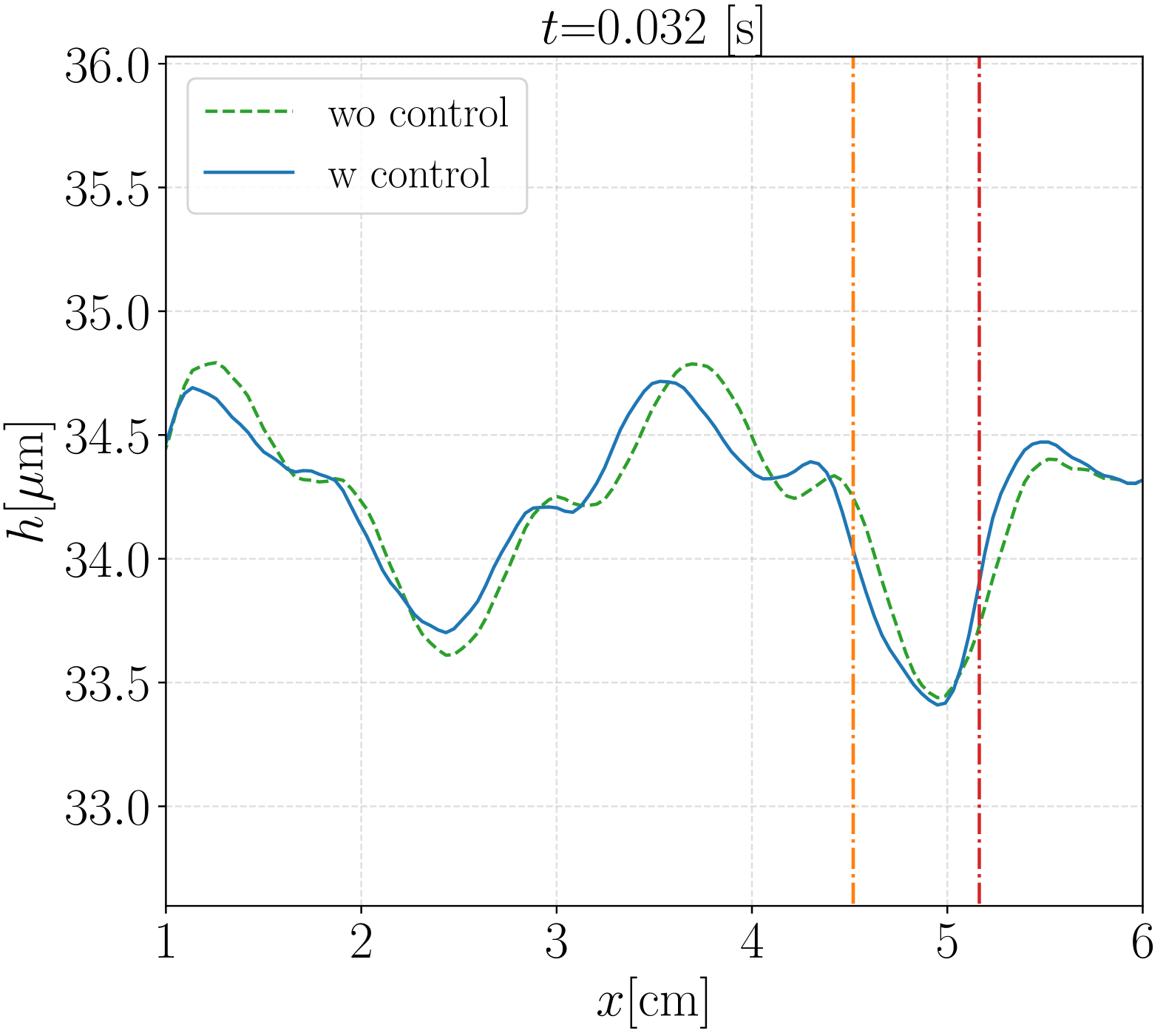
The control mechanism, which combines pushing crests and raising valleys, is most apparent when examining the evolution of the liquid film along a line in the streamwise direction. Figure 21 shows the evolution of the liquid film with control (solid blue line) and without control (dashed green line) along at . For a single actuator, the gas jets push down the crests with additional wiping. However, this is counteracted by the action of the electromagnet, resulting in waves with a smaller peak-to-valley amplitude in the controlled case compared to the uncontrolled one.
VIII Conclusion and Perspectives
In this study, we developed a 3D Integral Boundary Layer model to describe a liquid film on a moving substrate under the effect of a transverse magnetic field. The model was implemented in a numerical environment using the Fourier pseudo-spectral method. To reproduce open-domain conditions, we applied a linear, perfectly matched layer around the boundaries to absorb the incoming waves. Leveraging this numerical environment, we addressed a control problem involving unstable waves interacting with gas-jet and electromagnetic actuators. The optimal control law for the actuators was found using a reinforcement learning algorithm called proximal policy optimisation (PPO).
The Boundary Layer model exhibits good consistency with the non-magnetic model. As the magnetic field intensity decreases, the flat film steady-state solution and the closure relations for the flux terms and wall shear stress converge to their non-magnetic solutions.
Our analysis of the unsteady model at the leading order revealed that the convective velocity is always negative for . This highlights the strong influence that the magnetic field could have on the absolute and convective nature of steady-state solutions, further investigation of which could provide valuable insight into whether small defects on the free surface could impact industrial production processes. In addition, our study suggests that an effective magnetic field requires for galvanising conditions, which may be impractical for real-world applications due to high thermal gradients caused by the Joule effect and the destabilising magnetic effects on the strip’s dynamics.
Concerning the control problem, this study shows that an electromagnetic feedback regulator can effectively reduce unwanted wave amplitudes by raising their valleys. This outcome was achieved through a control mechanism governed by the resistive effects of the Lorentz force. These results open new avenues for applying this technique to more complex scenarios, particularly when considering the heat effects induced by the electromagnetic field, which could help to stabilise the liquid film via the Marangoni effects.
A key feature of our model is the absence of a hysteresis term in the magnetic field. In practice, the magnetic field does not change instantaneously when is adjusted; rather, it exhibits a response time determined by the magnetic properties of the solenoid’s core material. Although this simplification is sufficient for the accuracy required in this study, a more advanced model would need to account for the hysteresis effect. Another promising direction for future research could involve examining the effects of a high-frequency magnetic field, which could generate a ‘skin effect’, concentrating the induced electric current in a small region near the free surface.
This investigation provides valuable insights into the dynamics of the coating process, capturing the intricate multiscale interactions between the liquid zinc and control actuators at a computational cost lower than that of Large Eddy Simulations (LES). Beyond its immediate applications, the model can be adapted to other engineering problems. This opens new avenues for modelling, experimental investigations, and control design, ranging from ‘liquid walls’ used to confine plasma in tokamak nuclear fusion reactors to shaping versatile circuitry for next-generation electronic devices.
Appendix A Magnetohydrodynamic governing equations and boundary conditions
The liquid film is governed by the 3D incompressible Navier-Stokes equations given by:
| (58a) | |||
| (58b) | |||
where is the Lorentz force given by the interaction between the magnetic field in the liquid and the induced current. The relative motion of the liquid zinc with respect to the external magnetic field generates an induced current in the bulk , given by the Faraday’s law of induction neglecting the electric potential difference [37]:
| (59) |
The interaction of the induced current with results in a Lorentz force given by the cross product of and :
| (60) |
At the strip surface (), we enforce the non-slip condition:
| (61) |
At the free surface (), we impose the kinematic boundary condition:
| (62) |
along with the dynamic condition:
| (63) |
where is the free surface mean curvature [16, Chapter 2], defines the jump at the interface between the liquid and the gas phases, is the viscous stress tensor, and is the Maxwell stress tensor [55, Section 3.9] defined as:
| (64) |
By introducing the following notations:
| (65a) | |||
| (65b) | |||
| (65c) | |||
where is the strain-rate tensor, we obtain the three scalar equations representing the projections of the force balance (63) in the local Cartesian reference frame (O;) (defined in (2)):
| (66a) | |||
| (66b) | |||
| (66c) | |||
Appendix B Approximated magnetic field of a circular finite-length solenoid
This section details the assumptions behind the derivation of the approximated Gaussian magnetic field (31) presented in Subsection IV.2.
We consider a circular solenoid with radius and length , as illustrated in Figure 4, with a cylindrical reference frame centred at its midpoint. The analytical expression for the axial and radial components of the generated magnetic field read [43]:
| (68a) | |||
| (68b) |
where , , and are the complete elliptic integrals of the first, second, and third kinds, respectively, is the magnetic field at the solenoid’s core in the limit of given by:
| (69) |
where is the magnetic permeability of the core material, is the number of coils and is the electric current flowing through the coils of the solenoid. The variables , , and are expressed in terms of and by the following expressions:
| (70a) | |||
| (70b) | |||
| (70c) |
with and reading:
| (71) |
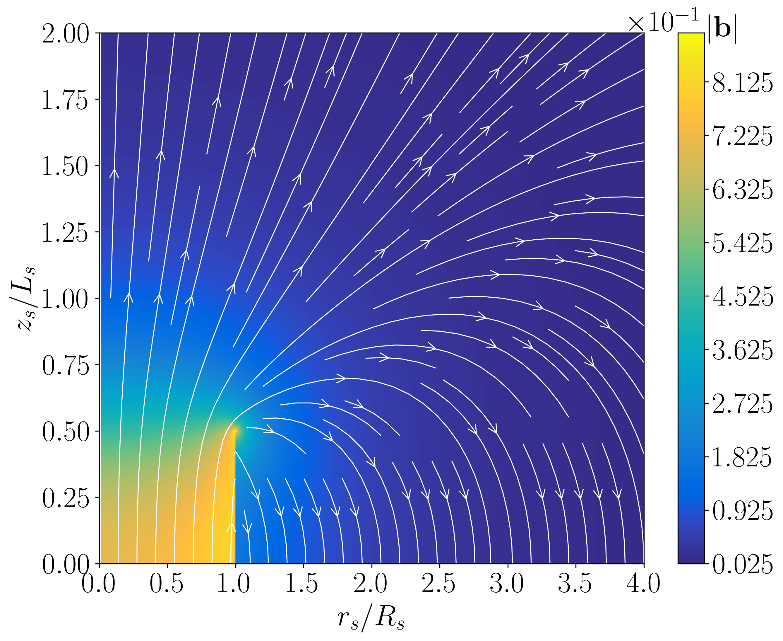
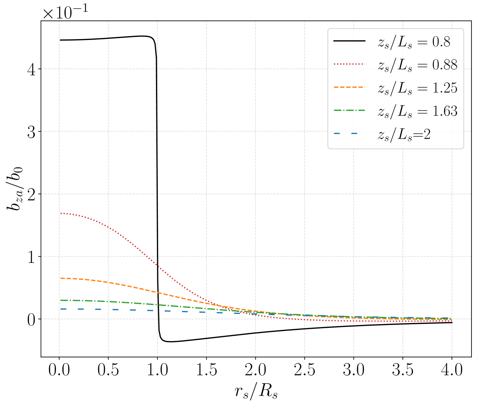
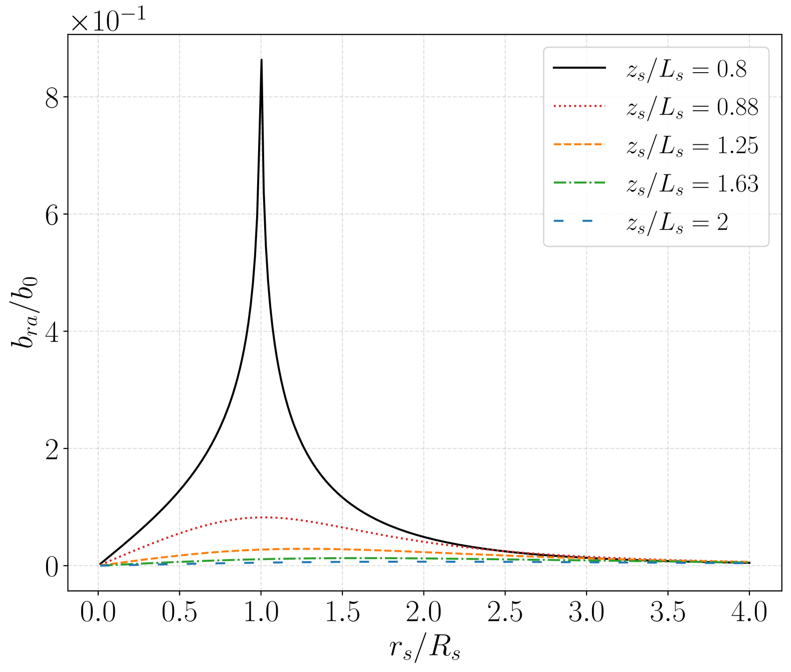
Figure 22 shows the normalized magnetic field (colour map) and magnetic field lines (white continuous lines), and figure and 23 shows the radial distributions of (a) the axial and (b) radial components of the magnetic field normalized with at different axial positions, , outside the solenoid. The field intensity drops sharply outside the solenoid, falling below of for and . Near the solenoid exit (), remains nearly constant along , while exhibits a peak at the edge (), where the field lines are most curved. As increases, both and become smoother, adopting a bell-shaped profile in , with the axial component dominating, being one order of magnitude larger than the radial component.
Based on these observations, assuming that the electromagnetic actuator is positioned far enough from the moving substrate, we neglected the radial component of the magnetic field and approximated its axial component as a Gaussian function in space, modulated by a time-varying amplitude , reading:
| (72) |
To define a relationship between the Gaussian’s standard deviation , the amplitude and the geometrical and physical characteristics of the solenoid , , and , we assume that or , where . Thereby, the complete elliptic integral of the third kind reduces to . This simplification leads to a more tractable expression for the axial magnetic field (68a), which reads:
| (73) |
At this point, we further assume that and which results in the following conditions for :
| (74) |
and for :
| (75) |
Leveraging this assumption, we can approximate and which simplify (73) into:
| (76) |
The difference in terms of absolute value between (76) with approximated by its first two terms in its power series expansion and the Taylor expansion of the approximated magnetic field (72) truncated at its fifth order around gives the error function , which reads:
| (77) |
To minimize , the coefficients at and are set to zero, yielding the following expressions for and :
| (78) |
where their nondimensional forms are reported in subsection IV.2.
Replacing in (78) with its definition (69) gives a relation between and the evolution of the electric current in the solenoid in time:
| (79) |
Concerning the magnetic field in the radial direction in (68b), it is straightforward to observe that this can be considered negligible with the approximation reported above.
Appendix C Governing and auxiliary equations implemented in the spectral BLEW 3D environment
Here, we report the modified governing and auxiliary differential equations arising from the perfectly matched layer transformation. The modified 3D IBL equations, without considering Maxwell stresses, with the auxiliary variable arising from the PML formulation reads:
| (80a) | |||
| (80b) | |||
| (80c) |
with the new set of auxiliary differential equations given by:
| (81) | ||||||
Acknowledgements.
F. Pino was supported by an F.R.S.-FNRS FRIA grant. This project was funded by Arcelor-Mittal Research. B. Scheid is Research Director at F.R.S.-FNRS.References
- Lalli and Giusti [2024] N. S. Lalli and A. Giusti, Journal of Fluid Mechanics 986, A7 (2024).
- Dumont et al. [2011a] M. Dumont, R. Ernst, Y. Fautrelle, B. Grenier, J. Hardy, and M. Anderhuber, COMPEL-The international journal for computation and mathematics in electrical and electronic engineering 30, 1663 (2011a).
- Pino et al. [2025] F. Pino, B. Scheid, and M. A. Mendez, Journal of Engineering Mathematics 150, 20 (2025).
- Lehman [1994] A. F. Lehman, in International Symposium on Electromagnetic Processing of Materials, 1994, Nagoya, ISIJ (1994).
- Zakharov [2003] L. E. Zakharov, Physical review letters 90, 045001 (2003).
- Narula et al. [2005] M. Narula, A. Ying, and M. Abdou, Fusion science and technology 47, 564 (2005).
- Morley et al. [2004] N. Morley, S. Smolentsev, R. Munipalli, M.-J. Ni, D. Gao, and M. Abdou, Fusion Engineering and Design 72, 3 (2004).
- Lunz and Howell [2019] D. Lunz and P. Howell, Journal of Fluid Mechanics 867, 835 (2019).
- Smolentsev et al. [2021] S. Smolentsev, T. Rhodes, Y. Jiang, P. Huang, and C. Kessel, Fusion Science and Technology 77, 745 (2021).
- Munipalli et al. [2003] R. Munipalli, S. Shankar, M. Ni, and N. Morley, DOE SBIR phase-ii final report (2003).
- Smolentsev and Abdou [2005] S. Smolentsev and M. Abdou, Applied mathematical modelling 29, 215 (2005).
- Seric et al. [2014] I. Seric, S. Afkhami, and L. Kondic, Journal of Fluid Mechanics 755, R1 (2014).
- Shkadov [1968] V. Y. Shkadov, Fluid Dynamics 3, 12 (1968).
- Kapitza [1949] S. Kapitza, Sov. Phys., J. Exp. Theor. Phys 19, 105 (1949).
- Ruyer-Quil et al. [2014] C. Ruyer-Quil, N. Kofman, D. Chasseur, and S. Mergui, The European Physical Journal E 37, 1 (2014).
- Kalliadasis et al. [2011] S. Kalliadasis, C. Ruyer-Quil, B. Scheid, and M. G. Velarde, Falling liquid films, vol. 176 (Springer Science & Business Media, 2011).
- Mendez et al. [2021] M. A. Mendez, A. Gosset, B. Scheid, M. Balabane, and J.-M. Buchlin, Journal of Fluid Mechanics 911, A47 (2021).
- Barreiro-Villaverde et al. [2021] D. Barreiro-Villaverde, A. Gosset, and M. A. Mendez, Physics of Fluids 33, 062114 (2021).
- Buchlin [1997] J.-M. Buchlin, Thin liquid films and coating processes (1997).
- Gosset et al. [2019] A. Gosset, M. A. Mendez, and J.-M. Buchlin, Experimental Thermal and Fluid Science 103, 51 (2019).
- Mendez et al. [2015] M. A. Mendez, K. Myrillas, A. Gosset, and J. Buchlin, in 11th European Coating Symposium (Eindhoven, The Netherlands, 2015).
- Mendez et al. [2019] M. Mendez, A. Gosset, and J.-M. Buchlin, Experimental Thermal and Fluid Science 106, 48 (2019).
- Barreiro-Villaverde et al. [2023] D. Barreiro-Villaverde, A. Gosset, M. Lema, and M. A. Mendez, Physics of Fluids 35 (2023).
- Barreiro-Villaverde et al. [2024a] D. Barreiro-Villaverde, A. Gosset, M. Lema, and M. A. Mendez, Journal of Fluid Mechanics 992 (2024a), ISSN 1469-7645.
- Mirhoseini et al. [2017] S. Mirhoseini, R. Diaz-Pacheco, and F. Volpe, arXiv preprint arXiv:1702.01040 (2017).
- Mirhoseini and Volpe [2016] S. Mirhoseini and F. Volpe, Plasma Physics and Controlled Fusion 58, 124005 (2016).
- Schulman et al. [2017] J. Schulman, F. Wolski, P. Dhariwal, A. Radford, and O. Klimov, arXiv preprint arXiv:1707.06347 (2017).
- Viquerat et al. [2022] J. Viquerat, P. Meliga, A. Larcher, and E. Hachem, Physics of Fluids 34 (2022).
- Vu et al. [2022] V. T. Vu, Q. H. Tran, T. L. Pham, and P. N. Dao, International Journal of Control, Automation and Systems 20, 1029 (2022).
- Zheng et al. [2021] M. Zheng, Y. Wu, and C. Li, Aerospace Science and Technology 119, 107126 (2021).
- Ran et al. [2021] M. Ran, J. Li, and L. Xie, IEEE Transactions on Cybernetics 52, 9621 (2021).
- Pino et al. [2023] F. Pino, L. Schena, J. Rabault, and M. A. Mendez, Journal of Fluid Mechanics 958, A39 (2023).
- Belus et al. [2019] V. Belus, J. Rabault, J. Viquerat, Z. Che, E. Hachem, and U. Reglade, AIP Advances 9, 125014 (2019).
- Ivanova et al. [2023] T. Ivanova, F. Pino, B. Scheid, and M. A. Mendez, Physics of Fluids 35 (2023).
- Giordanengo et al. [2000] B. Giordanengo, A. B. Moussa, A. Makradi, H. Chaaba, and J. Gasser, Journal of Physics: Condensed Matter 12, 3595 (2000).
- Gosset and Buchlin [2006] A. Gosset and J.-M. Buchlin, Journal of Fluids Engineering 129, 466 (2006).
- Dumont et al. [2011b] M. Dumont, R. Ernst, Y. Fautrelle, B. Grenier, J. J. Hardy, and M. Anderhuber, COMPEL - The International Journal for Computation and Mathematics in Electrical and Electronic Engineering 30, 1663 (2011b).
- Kapitza and Haar [1967] P. L. Kapitza and D. t. Haar, (No Title) (1967).
- Shkadov [1967] V. Y. Shkadov, Fluid Dynamics 2, 29 (1967).
- Beltaos and Rajaratnam [1974] S. Beltaos and N. Rajaratnam, Journal of the hydraulics division 100, 1313 (1974).
- Lacanette et al. [2006] D. Lacanette, A. Gosset, S. Vincent, J.-M. Buchlin, and É. Arquis, physics of Fluids 18, 042103 (2006).
- Bradshaw and Love [1959] P. Bradshaw and E. M. Love (1959).
- Hampton et al. [2020] S. Hampton, R. Lane, R. Hedlof, R. Phillips, and C. A. Ordonez, AIP Advances 10 (2020).
- Buck and Hayt [2011] J. Buck and W. Hayt, Engineering Electromagnetics (McGraw-Hill Education, 2011), ISBN 9780073380667, URL https://books.google.co.uk/books?id=XeaHcgAACAAJ.
- Dutykh [2016] D. Dutykh, arXiv preprint arXiv:1606.05432 (2016).
- Canuto et al. [2007] C. Canuto, M. Y. Hussaini, A. Quarteroni, and T. A. Zang, Spectral methods: evolution to complex geometries and applications to fluid dynamics (Springer Science & Business Media, 2007).
- Raffin et al. [2021] A. Raffin, A. Hill, A. Gleave, A. Kanervisto, M. Ernestus, and N. Dormann, Journal of Machine Learning Research 22, 1 (2021), URL http://jmlr.org/papers/v22/20-1364.html.
- OpenAI [2025] OpenAI, Proximal policy optimization — spinning up documentation, https://spinningup.openai.com/en/latest/algorithms/ppo.html (2025), accessed: 2025-01-21.
- Johnson [2021] S. G. Johnson, arXiv preprint arXiv:2108.05348 (2021).
- Besse et al. [2022] C. Besse, S. Gavrilyuk, M. Kazakova, and P. Noble, Water Waves 4, 313 (2022).
- Barreiro-Villaverde et al. [2024b] D. Barreiro-Villaverde, A. Gosset, M. Lema, and M. A. Mendez, Journal of Fluid Mechanics 992, A11 (2024b).
- Filip et al. [2019] S. Filip, A. Javeed, and L. N. Trefethen, SIAM Review 61, 185 (2019).
- Derjaguin [1943] B. V. Derjaguin, Acta Physicochim. URSS 20, 349 (1943).
- Pino et al. [2024] F. Pino, M. A. Mendez, and B. Scheid, Journal of Fluid Mechanics 1000, A57 (2024).
- Davidson [2001] P. A. Davidson, An Introduction to Magnetohydrodynamics, Cambridge Texts in Applied Mathematics (Cambridge University Press, 2001).