Pushing Everything Everywhere All At Once: Probabilistic Prehensile Pushing

Abstract

We address prehensile pushing, the problem of manipulating a grasped object by pushing against the environment. Our solution is an efficient nonlinear trajectory optimization problem relaxed from an exact mixed integer non-linear trajectory optimization formulation. The critical insight is recasting the external pushers (environment) as a discrete probability distribution instead of binary variables and minimizing the entropy of the distribution. The probabilistic reformulation allows all pushers to be used simultaneously, but at the optimum, the probability mass concentrates onto one due to the entropy minimization. We numerically compare our method against a state-of-the-art sampling-based baseline on a prehensile pushing task. The results demonstrate that our method finds trajectories 8 times faster and at a 20 times lower cost than the baseline. Finally, we demonstrate that a simulated and real Frank Panda robot can successfully manipulate different objects following the trajectories proposed by our method. Supplementary materials are available at https://probabilistic-prehensile-pushing.github.io/.

I Introduction

Prehensile pushing, exemplified in Fig. LABEL:fig:pull_figure, is the task of manipulating grasped objects by pushing them against external pushers (the environment) [1]. Finding pushing strategies is challenging because of the non-continuous, non-linear dynamics arising from contacts breaking and forming [2, 3, 4, 5]. The non-continuity, in particular, discourages gradient-based solutions because the optimization problem turns into an NP-hard Mixed Integer Nonlinear Program (MINLP), which is slow to solve [6]. As a result, many prior works have addressed the problem using gradient-free sampling-based methods [7, 8, 9]. Still, sampling-based methods are slow at finding solutions and include many hyper-parameters that must be tuned.

In this work, we formulate prehensile pushing as a mixed-integer non-linear trajectory optimization problem where pushers are binary integer variables and Motion Cones [7] are used to calculate admissible prehensile pushes given frictional contact. Furthermore, we propose an efficient continuous non-linear relaxation of the mixed-integer formulation, where the critical insight is recasting the integer variables as a discrete probability distribution and then minimizing the entropy of this distribution. Effectively, the relaxation allows all pushers to be used simultaneously, while the entropy term encourages the optimal solution to converge to one distinct pusher. The continuous relaxation is faster to solve and, for specific instances of our problem, will have the same global minimum as the original MINLP.

We compare our method numerically against the state-of-the-art MC-based Rapidly Exploring Random Tree (RRT) planner from Chavan et al. [7] on planar non-horizontal prehensile pushing tasks. The results demonstrate that our method finds, on average, a feasible trajectory 8 times faster and at a 20 times lower cost than the baseline. Finally, we validate our method on a simulated and real-world (Fig. LABEL:fig:pull_figure) prehensile pushing task. In summary, we contribute:

• An exact MINLP trajectory optimization formulation for prehensile pushing presented in Section V-A.

• The continuous Nonlinear Program (NLP) relaxation described in Section V-B.

• Auxiliary optimization objectives and optimization variables that reduce the pusher switching and speed up the program, presented in Section V-C.

• A comprehensive experimental evaluation demonstrating our method’s efficacy and real-world applicability, presented in Section VI.

We start by summarizing the related work, followed by the theoretical framework and problem statement.

II Related Work

Extrinsic dexterity [10] may include pushing against external contact, harnessing gravity, and executing dynamic arm motions. Solutions for extrinsic dexterity are mainly learning-based, sampling-based, or optimization-based, so we review them separately.

II-A Learning-Based

The prevailing learning methods for extrinsic dexterity are Reinforcement Learning (RL) [11, 12, 13, 14, 15] and Behavior Cloning (BC) [16]. The RL-based methods have mainly focused on object pivoting by either learning direct actions [11, 12, 14] or combining predefined manipulation primitives to pivot an object [15]. BC has been used to learn non-prehensile manipulation from videos [16]. Recently, some works have theoretically shown that RL is suitable for learning dexterous manipulation as it stochastically approximates the non-smooth contact dynamics [17, 18]. Thus, the main benefit of learning is that the non-trivial dynamics are implicitly learned rather than explicitly modeled. However, the downside of RL is that training is sample-inefficient, and learning often requires fine-tuned rewards, while BC requires high-quality demonstrations.

II-B Sampling-Based

If the contact dynamic is explicitly known, we can use it to plan dexterous manipulation through sampling-based or optimization-based methods. Many works [7, 8, 9, 4] have proposed different sampling-based methods as these can better handle the non-continuous contact dynamics than optimization-based methods. Out of these works, [7, 8, 4] uses different RRT-type samplers to find a set of pushes that would bring an object from a start to a goal pose. In contrast, the authors of [9] proposed a fast hierarchical planning framework that combines Monte Carlo Tree Search (MCTS), RRT, and contact dynamics.

The sampling-based method most similar to our work is [7], which uses MCs in the propagation step of a RRT. Our solution also builds upon the MC framework but integrates it into a gradient-based trajectory optimization formulation. The primary benefit of our solution over [7] is computational speed.

II-C Optimization-Based

The main challenge for optimization-based methods is the non-smooth contact dynamic that creates discontinuities in the optimization landscape. Some methods [19, 20, 21, 22, 23, 24] overcome the problem by smoothly approximating the contact dynamics by allowing contacts to act at a distance. Another more physically realistic solution is to model the planning-through-contact problem using complementarity constraints that ensure forces are only non-zero when there is contact [25, 26, 5].

The abovementioned methods solve the trajectory to local optimality, which is significantly easier than to solve for global optimality. There exist some approaches for finding globally optimal contact-rich trajectories [27, 28, 29, 30, 31, 32]. All these approaches, except [27], formulate the optimization problem as a Mixed Integer Program (MIP) that jointly optimizes over discrete contact modes and continuous robotic motions. In comparison, Graesdal et al. [27] frames the problem as finding the shortest path in a graph of convex sets. We formulate trajectory optimization as a MINLP, which we relax into a computationally cheaper NLP.

The main difference between our and other optimization-based methods is that we optimize over object twists instead of forces or accelerations. This is possible because the MCs provides direct dynamic feasibility bounds in the motion space.

III Preliminaries

Here, we describe MCs, later used as velocity constraints in our trajectory optimization formulation. The goal is to determine the possible object motions for stable pushing of an object while sliding on a support, as previously described in  [33, 7]. We do not contribute to the MC framework but present it here for completeness.

Consider a 2D rigid object $\mathbf{O}$ with a body-fixed coordinate frame $O$ whose origin is at the center of mass. Let ${\prescript{\text{O}}{}{\mathbf{w}_{\text{c}}}=\left[\prescript{\text{O}}{}{\mathbf{f}_{\text{c}}}^{\mathsf{T}},\prescript{\text{O}}{}{\mathbf{\tau}_{\text{c}}}^{\mathsf{T}}\right]^{\mathsf{T}}\in\mathbb{R}^{3}}$ denote the wrench applied by a contact $c$ and represented in the object frame $O$, as the stacked vector of contact force $\prescript{\text{O}}{}{\mathbf{f}_{\text{c}}}$ and torque $\prescript{\text{O}}{}{\mathbf{\tau}_{\text{c}}}$. The object is in frictional contact with a support $s$, with the origin of the support contact frame $S$ located at the center of pressure. In this work, the support is the gripper. A pusher $p$ that interacts with the object is represented by $k=1,\ldots,K$ frictional point contacts $p_{k}$. The origin of each local friction contact frame $P_{k}$ lies at the respective contact point. Unless otherwise specified, we denote quantities in the object frame $O$.

In the present planar scenario, pushing and sliding forces act upon the object within the same plane. Under the quasistatic assumption, i.e., sufficiently slow velocities, inertial effects can be neglected. Then, force balance holds:

$$\mathbf{w}_{\text{p}}+\mathbf{w}_{\text{s}}+m\mathbf{g}=\mathbf{0},$$ (1)

with $\mathbf{w}_{\text{p}}$ as pusher contact wrench, $\mathbf{w}_{\text{s}}$ as support wrench, $m$ as mass of the object, and $\mathbf{g}$ as gravitational force.

Following [33], a push is considered stable if contact between the pusher and the object is maintained throughout the motion. Considering friction adhering to Coulomb’s law of friction, pushing forces that result in sticking motion at a contact $p_{\text{k}}$ are constrained to lie within a friction cone $FC_{\text{p}_{k}}$. The contact normal force $\prescript{\text{P}_{k}}{}{\mathbf{n}_{\text{p}_{k}}}$ defines the cone’s axis of rotation, while the constant friction coefficient $\mu_{\text{p}}$ determines the opening angle $\beta=\arctan(\mu_{\text{p}})$. $\mu_{\text{p}}$ is assumed the same in static and kinetic friction cases. These local effects can be expressed via generalized friction cones in the object’s wrench space [34]. For a pusher $p$, the generalized friction cone is defined as the convex hull:

$$\mathbf{W}_{\text{p}}=\left\{\hat{\mathbf{w}}_{\text{p}_{k}}=\text{Ad}_{\mathbf{T}_{\text{P}_{k}O}}^{\mathsf{T}}\prescript{\text{P}_{k}}{}{\hat{\mathbf{f}}_{\text{p}_{k}}}\;|\;\prescript{\text{P}_{k}}{}{\hat{\mathbf{f}}_{\text{p}_{k}}}\in FC_{\text{p}_{k}},\;\forall k\right\},$$ (2)

where the unit wrench applied by a pusher contact $\hat{\mathbf{w}}_{\text{p}_{k}}$ corresponds to the effect of a unit force $\hat{\mathbf{f}}_{\text{p}_{k}}$ on the object. The adjoint transformation $\text{Ad}_{\mathbf{T}_{\text{P}_{k}O}}^{\mathsf{T}}$ maps the local pusher contact forces to wrenches in the object frame.

The maximum set of wrenches on the object by the support contact $\prescript{\text{S}}{}{\mathbf{w}_{\text{s}}}$ that can be statically transmitted is strictly bounded by an ellipsoidal limit surface. A contact wrench intersecting the limit surface results in a quasistatic sliding motion. The unit support wrench, $\prescript{\text{S}}{}{\hat{\mathbf{w}}_{\text{s}}}=\>\prescript{\text{S}}{}{\mathbf{w}_{\text{s}}}(\mu_{\text{s}}F_{N})^{-1}$, is proportional to the friction coefficient $\mu_{\text{s}}$ that arises between the object and the support, and magnitude of support normal force $F_{N}$. It defines the ellipsoidal limit surface as:

$$\prescript{\text{S}}{}{\hat{\mathbf{w}}_{\text{s}}}^{\mathsf{T}}\mathbf{A}\prescript{\text{S}}{}{\hat{\mathbf{w}}_{\text{s}}}=1,$$ (3)

with $\mathbf{A}=\text{diag}(\left[1,1,(re)^{-2}\right])$. Here, $r$ is the radius of the support contact, and $e\in\left[0,1\right]$ is an integration constant specifying the pressure distribution at the support contact interface.

Combining equations (1) and (2), the force balance condition for a stable push on a sliding object is obtained as:

$$a\hat{\mathbf{w}}_{\text{p}}+(\mu_{\text{s}}F_{N})\>\text{Ad}_{\mathbf{T}_{SO}}^{\mathsf{T}}\prescript{\text{S}}{}{\hat{\mathbf{w}}_{\text{s}}}+m\mathbf{g}=0,$$ (4)

where $\hat{\mathbf{w}}_{\text{p}}\in\mathbf{W}_{\text{p}},\;a\in\mathbb{R}^{+}$. The unit pusher wrench inside the generalized friction cone $\hat{\mathbf{w}}_{\text{p}}\in\mathbf{W}_{\text{p}}$ is scaled by a magnitude $a$. Note that the magnitude of the support normal force $F_{N}$ and the design parameters $\mu_{s}$ and $e$ influence the unique solution of $a$.

Solving equations (3) and (4) together yields a set $\prescript{\text{S}}{}{\mathbf{W}_{\text{s}}}$, which effectively constrains the admissible support contact wrenches $\prescript{\text{S}}{}{\hat{\mathbf{w}}_{\text{s}}}\in\prescript{\text{S}}{}{\mathbf{W}_{\text{s}}}$ during stable pushing of a sliding object. For a uniform and finite support friction distribution, the resulting sliding velocity from such a frictional contact wrench is normal to its intersection point with the limit surface [35]. Hence, the direction of the velocity can be obtained via differentiation of (3). Let the object motion w.r.t. the support frame be denoted by the twist $\prescript{\text{S}}{}{\bm{\xi}_{\text{o}}}=\left[\prescript{\text{S}}{}{\mathbf{v}_{\text{o}}}^{\mathsf{T}},\prescript{\text{S}}{}{\mathbf{\omega}_{\text{o}}}^{\mathsf{T}}\right]^{\mathsf{T}}\in\mathbb{R}^{3}$, with linear velocity $\prescript{\text{S}}{}{\mathbf{v}_{\text{o}}}$ and angular velocity $\prescript{\text{S}}{}{\mathbf{\omega}_{\text{o}}}$. Then, the set of possible object motions resulting from stable pushes is defined as the motion cone:

$$\prescript{\text{S}}{}{\mathbf{V}_{\text{o}}}=\left\{\prescript{\text{S}}{}{\bm{\xi}_{\text{o}}}=b\mathbf{A}\prescript{\text{S}}{}{\hat{\mathbf{w}}_{\text{s}}}\;|\;\prescript{\text{S}}{}{\hat{\mathbf{w}}_{\text{s}}}\in\prescript{\text{S}}{}{\mathbf{W}_{\text{s}}},b\in\mathbb{R}^{+}\right\},$$ (5)

with velocity scaling factor $b$. Note that the wrench is independent of the speed of motion [36]. An illustration of these preliminaries is provided in Figure 1.

\begin{overpic}[width=216.81pt]{Figures/mc.pdf}\put(25.0,470.0){\scriptsize P}\put(380.0,500.0){\scriptsize G}\put(380.0,300.0){\scriptsize{O}}\put(80.0,400.0){\scriptsize$p_{0}$}\put(80.0,300.0){\scriptsize$p_{1}$}\put(235.0,385.0){\scriptsize$O$}\put(390.0,380.0){\scriptsize$S$}\put(250.0,250.0){\scriptsize(a)}\put(130.0,10.0){\scriptsize(b)}\put(370.0,10.0){\scriptsize(c)}\put(570.0,10.0){\scriptsize(d)}\put(770.0,10.0){\scriptsize(e)}\put(770.0,250.0){\scriptsize(f)}\put(558.0,160.0){\scriptsize y}\put(540.0,65.0){\scriptsize z}\put(620.0,90.0){\scriptsize x}\put(310.0,390.0){\scriptsize x}\put(235.0,320.0){\scriptsize z}\par\end{overpic}

Figure 1: Visual description for calculating MCs. (a) Shows the pusher (P) pushing the rectangular object (O), which slides inside the gripper (G). Together, the convex hull of the generalized friction cones (b), the limit surface (c), and the gravity acting on the object (d) result in the motion resolution (e). The final polyhedral approximation of the motion cone is shown in (f). The axes labels in (b), (c), (e), and (f) follow the convention in (d), where forces act along the x- and z-axis and torque around the y-axis (best viewed in color).

To compute the motion cone, we follow [7] and first sweep over the boundaries of the pusher cone, obtain the boundaries of support and motion cone, and approximate the surfaces connecting supports linearly to end up with a polyhedral approximation of this motion cone. In our following formulation of the trajectory optimization problem, we rely on the computation of motion cones as the set of admissible object twists that will result in stable pushes and apply the motion cone as a constraint.

IV Problem Statement

Using the same notation as in the previous section, the problem we address is manipulating $\mathbf{O}$ from a start pose $\mathbf{P}_{0}\in\text{SE}(2)$ to a goal pose $\mathbf{P}_{g}\in\text{SE}(2)$ by sequentially pushing against external pushers $p^{0},\dots,p^{M}\in\{0,1\}$. The push action is a twist $\bm{\xi}$. The goal is reached when $d(\mathbf{P}_{N},\mathbf{P}_{g})\leq\epsilon$, where $d:\text{SE}(2)\times\text{SE}(2)\rightarrow\mathbb{R}_{\geq 0}$ is a distance function, $\mathbf{P}_{N}$ is the final pose and $\epsilon$ is a user-specified distance threshold. We define the distance function as $d(\mathbf{P}_{N},\mathbf{P}_{g})=\lambda_{s}\left\lVert\bm{\kappa}_{N}-\bm{\kappa}_{g}\right\rVert+\lambda_{\theta}\left\lvert\theta_{N}-\theta_{g}\right\rvert$, where $\bm{\kappa}\in\mathbb{R}^{2}$ is a position vector, $\theta$ is a rotation around the global coordinate system’s y-axis, and $\lambda_{s}$ and $\lambda_{\theta}$ are user-specified weights.

We represent $\mathbf{O}=\left\{\bm{\nu}_{0},\bm{\nu}_{1},\dots,\bm{\nu}_{I}\right\}$ with a set of vertices $\bm{\nu}_{i}\in\mathbb{R}^{2}$, where $\bm{\nu}_{i}$ is connected to $\bm{\nu}_{i+1}$ and $\bm{\nu}_{I}$ is connected to $\bm{\nu}_{0}$. We predefine the number of pushing sequences $N$ and the maximum execution time $T$, which are used to calculate the time-step for each push as $\delta=\frac{T}{N-1}$. Given these specifications, the problem becomes finding a sequence of pushers $p^{0},\dots,p^{M}$ and twists $\bm{\xi}_{0},\dots,\bm{\xi}_{N-1}$ that minimizes $d(\mathbf{P}_{N},\mathbf{P}_{g})$.

V Prehensile Pushing as Trajectory Optimization

We now present the MINLP formulation for prehensile pushing and then the computationally more tractable continuous NLP relaxation. Finally, we discuss additional cost and optimization variables used to speed up the optimization and find trajectories that are easier to execute on physical hardware.

V-A Mixed Integer Nonlinear Programming Formulation

We define the trajectory optimization problem as minimizing the distance between $\mathbf{P}_{N}$ and $\mathbf{P}_{g}$ while keeping the twists inside the motion cone and the pusher on the object. Mathematically, this is formulated as:

—s—ξ^m_n, P_n, p^m_n m∈{0,…,M}n∈{0,…,N-1} ∥P_N - P_g∥+λ_p ∑_n=0^N-1 ∥P_n+1 - P_n∥, ξ_n^m ∈^S_V_o,n^m P_n ∈O P_n+1= P_n+δ∑_m = 0^M ξ_n^mp_n^m ∑_m = 0^M p_n^m = 1 p_n^m ∈{0,1}, where $n$ describes the discretization point of the trajectory, $\bm{\xi}^{m}_{n}$ is the m-th twist at the n-th segment, $\prescript{\text{S}}{}{\mathbf{V}_{o,n}^{m}}$ is the m-th motion cone at the n-th segment, $p_{n}^{m}$ is the m-th pusher at the n-th segment, and $\lambda_{p}$ is a user-specified weighting term. In the above optimization problem, Eq. V-A ensures the twist is inside the MC, Eq. V-A ensures the gripper is on the object, Eq. V-A ensures the dynamics hold, and Eq. V-A and Eq. V-A combined ensure that one and only one pusher is active.

If $\mathbf{O}$ is convex, we can express Eq. V-A as the linear constraint:

$$\mathbf{A}\begin{pmatrix}x_{n}\\ y_{n}\end{pmatrix}\leq\mathbf{b},$$ (6)

where $\mathbf{A}\in\mathbb{R}^{I\times 2}$ and $\mathbf{b}\in\mathbb{R}^{I}$ are derived from the vertices of $\mathbf{O}$ and $x_{n}$ and $y_{n}$ are the 2D position of $\mathbf{P}_{n}$. Non-convex $\mathbf{O}$ cannot be expressed in the same linear form. Instead, for such objects, we first divide the object into a set of convex regions $\{\mathbf{U}_{0},\dots,\mathbf{U}_{L}|\bigcup_{l=0}^{L}\mathbf{U}_{l}=\mathbf{O}\}$ where each $\mathbf{U}_{l}$ is associated with a linear state-constraint $\mathbf{A}_{l}\begin{pmatrix}x_{n}\\ y_{n}\end{pmatrix}-\mathbf{b}_{l}\leq 0$ and a binary variable $\psi_{l}\in\{0,1\}$ that is 1 iff $\mathbf{P}_{n}\in\mathbf{U}_{l}$. Then, we can form the state constraint as the integer constraint:

$$\begin{split}\sum_{l=0}^{L}\psi_{l}&=1,\\ \psi_{l}\left[\mathbf{A}_{l}\begin{pmatrix}x_{n}\\ y_{n}\end{pmatrix}-\mathbf{b}_{l}\right]&\leq 0~\forall l\in\{0,\dots,L\}.\end{split}$$ (7)

The optimization problem in Eq. V-A is a MINLP due to the integer constraints (V-A) and (7), and the non-linear constraint (V-A). Unfortunately, MINLPs are NP-hard [6], meaning they are computationally expensive to solve. Thus, to make the problem computationally more tractable, we propose to continuously relax Eq. V-A into a NLP.

V-B Continuous Relaxation

We continuously relax the integer variables $p_{n}^{m}$ in Eq. V-A by treating them as probabilities. This reformulation has one obvious limitation: it allows for solutions where the robot simultaneously uses all pushers, which is physically impossible. Therefore, the probability mass should concentrate on one distinct $p_{n}^{m}$ at the optimum. To encourage this, we add the entropy of the discrete probability distribution as an additional cost term. Mathematically, the continuous relaxation of Eq. V-A becomes: —s— ξ^m_n, P_n, p^m_n m∈{0,…,M}n∈{0,…,N-1} ∥P_N - P_g∥ +λ_p ∑_n=0^N-1 ∥P_n+1 - P_n∥ + λ_e ∑_n=0^N-1∑_m=0^M p_n^mlog(p_n^m) (V-A)-(V-A) p_n^m ≥0, where $\lambda_{e}$ is a user-specified weighing term. Ideally, the entropy term in Eq. V-B concentrates the probability mass onto one pusher. Thus, once we execute the actual trajectory, we sample the most probable pushers as:

$$p_{n}^{*}=\operatorname*{arg\,max}_{m\in\{0,...,M\}}p_{n}^{m},~\forall n\in\{0,\dots,N\}.$$ (8)

Despite the rounding in Eq. 8 the constraints (V-A)-(V-A) remain feasible because 1. $\bm{\xi}_{n}^{m}\in\prescript{\text{S}}{}{\mathbf{V}_{o,n}^{m}}$is enforced during optimization, satisfying constraint (V-A), 2. $\mathbf{P}_{n}\in\mathbf{O}$is independent of the pusher selection, satisfying constraint (V-A), 3. the dynamics remain valid as we only execute motions corresponding to the selected pusher, satisfying constraint (V-A), and 4. exactly one pusher is selected at each timestep through the $\arg\max$ operation, satisfying constraint (V-A).

We propose to smooth the boundaries between the convex regions to relax the integer non-convex state-constraint (7). Specifically, for each neighboring convex regions $\mathbf{U}_{l}$ and $\mathbf{U}_{l+1}$ we add a Sigmoid function:

$$\sigma_{l}(x)=\frac{1}{1+\exp(-\alpha\cdot(x-\hat{x}_{l}))},$$ (9)

where $\hat{x}_{l}$ is the x-value between the two convex regions and $\alpha$ is a hyperparameter. Using the Sigmoid functions, we can formulate the continuous non-convex state constraint as:

$$\begin{split}(1-\sigma_{0}(x_{n}))(1-\sigma_{1}(x_{n}))\cdots(1-\sigma_{L-1}(x_{n}))f_{0}(x_{n},y_{n})+\\ \sigma_{0}(x_{n})(1-\sigma_{1}(x_{n}))\cdots(1-\sigma_{L-1}(x_{n}))f_{2}(x_{n},y_{n})+\dots+\\ \sigma_{0}(x_{n})\sigma_{1}(x_{n})\sigma_{L-1}(x_{n})f_{L-1}(x_{n},y_{n})\leq 0,\end{split}$$ (10)

where $f_{l}(x_{n},y_{n})=\mathbf{A}_{l}\begin{pmatrix}x_{n}\\ y_{n}\end{pmatrix}-\mathbf{b}_{l}$. By tuning $\alpha$ in Eq. 9, we can make the boundary infinitely steep, and at $\alpha\to\infty$, we recover the integer constraint in Eq. 7. Fig. 2 shows an example of the smoothed non-convex state constraint with only one $\sigma$.

Figure 2: The smoothed non-convex state constraint for the T-shaped object. Here, $\alpha=200$ and $\hat{x}_{0}=0.02$.

The relaxed problem can now be solved using gradient-based optimization in polynomial time. The relaxation in Eq. V-B is also conservative because it has the same global optimum as Eq. V-A, assuming such an optimum exists and that $N\to\infty$. This is true because the minimization of the entropy cost results asymptotically in a discrete probability distribution. The initial solution begins around the barycenter of the simplex and evolves towards one of the vertices, where only one mode remains active. Such vertex coincides with the global minimum of the original MINLP.

V-C Additional Improvements

Solving Eq. V-B already results in physically plausible trajectories that, once executed, manipulate the object. Still, we can further speed up the computation and ensure that the trajectories are more efficient to execute on a real robot if we (i) allow for variable execution time $T$, and (ii) minimize pusher switching.

Variable Time. Instead of prespecifying $T$, we add it as an additional optimization variable. Adding it gives the optimizer more freedom at the cost of an additional optimization variable and constraint $\delta=\frac{T}{N-1}$.

Pusher Switch Minimization. Eq. V-B allows for arbitrarily many pusher switches. However, on a real system where switching pushers is costly, the fewer, the better. We incorporate pusher switch minimization into Eq. V-B by adding the Kullback-Leibler (KL) divergence between consecutive probability distributions as a cost. Mathematically, we add the following objective

$$\lambda_{kl}\sum_{n=0}^{N-1}D_{KL}(p_{n+1}^{m}||p_{n}^{m}),$$ (11)

where $D_{KL}(p_{n+1}^{m}||p_{n}^{m})=\sum_{m=0}^{M}p_{n+1}^{m}\log\frac{p_{n+1}^{m}}{p_{n}^{m}}$.

Incorporating all the additional objectives and constraints results in the optimization problem: —s— ξ^m_n, P_n, p^m_n T m∈{0,…,M}n∈{0,…,N-1} ∥P_N - P_g∥ + λ_p ∑_n=0^N-1 ∥P_n+1 - P_n∥ +λ_e ∑_n=0^N-1∑_m=0^M p_n^mlog(p_n^m) +λ_kl∑_n=0^N-2∑_m=0^MD_KL(p_n+1^m——p_n^m) (V-A)-(V-A) p_n^m ≥0 δ=TN-1, where $\lambda_{p}$, $\lambda_{e}$, and $\lambda_{kl}$ are user-specified weighing terms for the separate loss functions.

VI Experiments

We experimentally evaluate our trajectory optimization formulation on a 2D non-horizontal prehensile pushing task. To solve the NLPs, we used the Sequential Least SQuares Programming optimizer (SLSQP) version 1.9.1 from SciPy [37]. We used the following hyperparameters in all experiments as they delivered the best performance: $N=3$, $\alpha=200$, $T=2$, $\lambda_{p}=\lambda_{e}=\lambda_{kl}=0.1$, $\lambda_{s}=0.9$, and $\lambda_{\theta}=0.1$. All computations are done on Ubuntu 20.04.5 LTS using an Intel Core i7-10750H 2.60GHz processor. $\mathbf{P}_{n}$ are initialized using linear interpolation between $\mathbf{P}_{0}$ and $\mathbf{P}_{N}$. The twists $\bm{\xi}^{m}_{n}$ are initialized using finite differencing $\bm{\xi}^{m}_{n}=\frac{1}{\delta}\log(\mathbf{P}_{n-1}^{-1}\mathbf{P}_{n})$. Pusher probabilities $p^{m}_{n}$ are initialized uniformly ($p^{m}_{n}=\frac{1}{M+1}$) to avoid bias towards any particular pusher.

The specific questions we wanted to answer with the experiments were:

1. What are the differences between our approach and RRT-MC regarding computational time and solution quality?

2. What effects do the variable time and switch minimization have on the computational efficiency and the solution?

3. How successful is a Franka Panda robot at manipulating objects when following trajectories generated by our method?

VI-A Numerical Evaluation

We numerically evaluated all methods on a convex squared object and a non-convex T-shaped and L-shaped object. We fixed the goal state for each object while uniformly sampling 20 different start states. An example of the start and goal states for the T-shape is shown in Fig. 3(a). The environment included four different pushers. We benchmarked against our implementation of the RRT-based MC method from [7], hereafter referred to as RRT-MC. We set $\epsilon=10^{-4}$.

(a)

(b)

Figure 3: (3(a)) shows the uniformly sampled start and goal positions while (3(b)) shows an optimized trajectory.

Figure 4: The relationship between the goal distance and the computational budget. T stands for the T-shaped and L for the L-shaped object.

The numerical results are shown in Fig. 4. The results demonstrate that, after 20 seconds, our method’s goal distance is 1,000 times smaller for the non-convex object and 10,000 times smaller for the convex one than RRT-MC. Even after running RRT-MC for 140 seconds on the convex and 160 seconds on the non-convex object, the distance to the goal is still 100 times higher than the solution our method provides after only 20 seconds. Fig. 3(b) shows an example trajectory found using our method.

We further analyzed how different optimization variables impact the computational time and the goal distance when optimizing Eq. V-B. The results are presented in Table I and demonstrate that the direct transcription formulation, where both $\bm{\xi}$ and $\mathbf{P}$ are optimized, leads to a ten times lower goal distance than single shooting methods that only optimize $\bm{\xi}$. Adding $T$ as an optimization variable reduces the computational time by 2–4 seconds.

Finally, we investigated if the KL-penalty in Eq. V-C reduced the number of pusher switches. To quantify the reduction in pusher switches, we propose the metric $Q=100\times\frac{\Delta-\Delta_{kl}}{\Delta}$, where $\Delta_{kl}$ and $\Delta$ are the total number of pusher switches with and without the KL penalty, respectively. The Q-metric represents the percentage reduction in pusher switches when using the KL penalty compared to not using it, where a higher value indicates fewer pusher switches. Fig. 5 illustrates the switch reduction as a function of $\mu$. The results demonstrate that with $\mu=0.4$, the KL penalty decreases pusher switching with $15\%$. As expected, the percentage of switches approaches zero as the friction coefficient increases because the MC becomes wide enough that object manipulation is possible using only one pusher.

TABLE I: Solution time and objective value for different optimization variables. T stands for the T-shaped and L for the L-shaped object.

Optimization Variables	Time (s)			Objective Value
	Square	T	L	Square	T	L
$\bm{\xi},~\mathbf{p}$	23	27	26	$e^{-6}$	$e^{-6}$	$e^{-6}$
$\bm{\xi},~\mathbf{p},~T$	20	23	23	$e^{-6}$	$e^{-6}$	$e^{-6}$
$\bm{\xi},~\mathbf{p},~\mathbf{P}$	34	39	37	$e^{-7}$	$e^{-6}$	$e^{-6}$
$\bm{\xi},~\mathbf{p},~\mathbf{P},~T$	31	37	36	$e^{-7}$	$e^{-7}$	$e^{-6}$

Figure 5: The reduction in switches w/ and w/o the KL penalty as a function of the friction coefficient $\mu$.

VI-B Evaluation in Physics Simulation

Next, we evaluate RRT-MC and our best method from the numerical experiments, namely Eq. V-C, in the physics engine MuJoCo [38]. The simulation environment includes a Frank Panda robot, the object to manipulate, and a free-floating fixture that serves as the external pusher. The end-effector twists were mapped to joint velocities using differential inverse kinematics. We performed a grid search over MuJoCo’s hyper-parameters to find a combination that enabled prehensile pushing. The selected hyper-parameters are detailed in Appendix A.

Each method generated five different trajectories for each object type (square, T-shaped, and L-shaped), using consistent pre-selected start and goal poses. The evaluation used two $\epsilon$ thresholds: $\epsilon=5^{-4}$ for high-precision control and $\epsilon=6^{-3}$ for standard operation. With the stricter threshold ($\epsilon=5^{-4}$), our method achieved successful manipulation in all trials (100% success rate), while RRT-MC failed to reach the target poses (0% success). When relaxing the threshold to $\epsilon=6^{-3}$, both methods achieved complete success (100%). These results demonstrate that our method can generate robust trajectories under realistic physics simulation, particularly for high-precision manipulation tasks.

VI-C Real World Evaluation

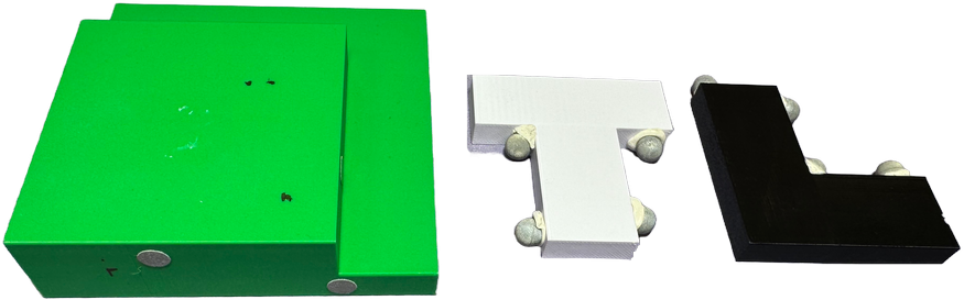
Figure 6: Objects for real-world experiments.

Finally, we conducted physical experiments using a Frank Panda to validate the real-world applicability of our approach. As in the simulation experiment, we evaluated our best method Eq. V-C. Our method was evaluated on the three objects in Fig. 6: a convex square and a non-convex T- and L-shape, with dimensions and weights listed in Table II. The objects’ poses were tracked using a motion capture system. The robot could use two different pushers. We set $\epsilon=10^{-4}$ and executed one trajectory per object.

The experimental results demonstrated successful manipulation from the start to the goal pose across all three object geometries. An example execution is presented in Fig. LABEL:fig:pull_figure, while the complete execution sequences are available at https://probabilistic-prehensile-pushing.github.io/. These real-world results confirm that the trajectories generated by our optimization approach are robust enough to transfer from planning to physical execution, even when subject to real-world factors such as friction variations, contact uncertainties, and robot control imperfections.

TABLE II: Object dimensions and weights.

Shape	Dim [L, W, H] (mm)		Mass (g)
Square		100, 20, 100		121
T-shape		60, 10, 35		47
L-shape		60, 10, 60		12

VII Discussion

Together, our experimental results demonstrate the advantages of our trajectory optimization approach over RRT-MC. The numerical evaluations show that our method finds solutions 8 times faster and achieves costs 20 times lower than RRT-MC. This improved performance translated directly to practical benefits, with our method achieving a 10x lower goal distance in simulation than RRT-MC. Furthermore, our real-world experiments validated that a physical robot can successfully reorient objects by following the trajectories proposed by our method.

While our method’s computation time of approximately 20 seconds precludes real-time feedback control, it offers several advantages. The main benefit is the flexibility to incorporate additional objectives and constraints. For instance, we demonstrated how pusher switches could be minimized by introducing the KL-cost term in (11). Implementing similar behavior modifications in sampling-based methods like RRT-MC would require non-trivial changes to the tree expansion strategy, potentially compromising exploration efficiency and further increasing computation time. Another benefit is our method’s reduced sensitivity to hyper-parameters compared to RRT-MC. We experimentally discovered that for RRT-MC, many step size and $\epsilon$ combinations resulted in overshooting behaviors where a solution was never found. In contrast, our optimization-based approach proved more robust across different parameter settings.

Finally, our probabilistic relaxation of mixed-integer constraints represents a novel theoretical contribution that could be valuable beyond this specific application. For instance, in cluttered pick-and-place scenarios, instead of making binary decisions about which objects to move, a planner could assign probabilities to different objects and smoothly explore various clearing sequences while naturally converging to discrete choices through entropy minimization.

Regarding the computation time, several directions exist for reducing it. One is to design a specialized solver that exploits the problem’s structure. Another is to relax the NLP in (V-B) into a convex problem, which could unlock millisecond solution rates. Finally, warm-starting techniques could be employed for faster re-planning in dynamic scenarios.

Another line of future work is combining RRT-MC and the trajectory optimization formulation. For instance, RRT-MC could generate diverse initial trajectories that our method then refines. This hybrid approach might prove valuable for more complex scenarios like bi-manual prehensile manipulation, where one end-effector is a movable pusher, and the other is a movable support [39]. A final suggestion for future work is to extend the proposed method to closed-loop estimation of friction parameters.

VIII Conclusion

This paper addressed the challenging task of prehensile pushing. Our solution formulated prehensile pushing as a non-linear trajectory optimization problem using MCs. The key idea was to relax the binary variables in the original MINLP into a discrete probability distribution and to penalize the entropy of said distribution, resulting in a quick-to-solve NLP. Although the probabilistic formulation allowed the robot to use all pushers simultaneously, the probability mass focused on one distinct pusher at the optimum due to the entropy minimization. The experimental evaluations demonstrated that our trajectory optimization method found solutions 8 times faster and at a 20 times lower cost than a state-of-the-art sampling-based baseline. Finally, we verified that a simulated and real-world Frank Panda robot could successfully reorient objects by following the trajectories proposed by our solution.

Appendix A

The following parameters simulated prehensile pushing in MuJoCo [38]. The numerical integrator was set to implicitfast, with a stepsize of $0.002$. We enabled the multiccd parameter to allow for multiple-contact collision detection between geom pairs and set condim to 6. The sliding, torsional, and rolling friction were set to 1.05, 0.05, and 0.1, respectively. The solimp parameters $d_{0}$, $d_{\text{width}}$, width, midpoint, and power were set to $1$, $0.5$, $0.2$, $0.5$, $2$, respectively. The solref parameters timeconst and dampratio were set to $0.001$ and $1$, respectively.

References

- [1] N. Chavan-Dafle and A. Rodriguez, “Prehensile pushing: In-hand manipulation with push-primitives,” in IEEE/RSJ International Conference on Intelligent Robots and Systems, 2015, pp. 6215–6222.
- [2] W. Yuan, J. A. Stork, D. Kragic, M. Y. Wang, and K. Hang, “Rearrangement with nonprehensile manipulation using deep reinforcement learning,” in 2018 IEEE International Conference on Robotics and Automation, 2018, pp. 270–277.
- [3] W. Yuan, K. Hang, D. Kragic, M. Y. Wang, and J. A. Stork, “End-to-end nonprehensile rearrangement with deep reinforcement learning and simulation-to-reality transfer,” Robotics and Autonomous Systems, vol. 119, pp. 119–134, 2019.
- [4] T. Pang, H. T. Suh, L. Yang, and R. Tedrake, “Global planning for contact-rich manipulation via local smoothing of quasi-dynamic contact models,” IEEE Transactions on robotics, 2023.
- [5] W. Jin and M. Posa, “Task-driven hybrid model reduction for dexterous manipulation,” IEEE Transactions on Robotics, 2024.
- [6] S. Burer and A. N. Letchford, “Non-convex mixed-integer nonlinear programming: A survey,” Surveys in Operations Research and Management Science, vol. 17, no. 2, pp. 97–106, 2012.
- [7] N. Chavan-Dafle, R. Holladay, and A. Rodriguez, “Planar in-hand manipulation via motion cones,” The International Journal of Robotics Research, vol. 39, no. 2-3, pp. 163–182, 2020.
- [8] N. Chavan-Dafle and A. Rodriguez, “Sampling-based planning of in-hand manipulation with external pushes,” in Robotics Research: The 18th International Symposium ISRR, 2020, pp. 523–539.
- [9] X. Cheng, S. Patil, Z. Temel, O. Kroemer, and M. T. Mason, “Enhancing dexterity in robotic manipulation via hierarchical contact exploration,” IEEE Robotics and Automation Letters, vol. 9, no. 1, pp. 390–397, 2023.
- [10] N. C. Dafle, A. Rodriguez, R. Paolini, B. Tang, S. S. Srinivasa, M. Erdmann, M. T. Mason, I. Lundberg, H. Staab, and T. Fuhlbrigge, “Extrinsic dexterity: In-hand manipulation with external forces,” in IEEE International Conference on Robotics and Automation, 2014, pp. 1578–1585.
- [11] W. Zhou and D. Held, “Learning to grasp the ungraspable with emergent extrinsic dexterity,” in Conference on Robot Learning. PMLR, 2023, pp. 150–160.
- [12] W. Zhou, B. Jiang, F. Yang, C. Paxton, and D. Held, “Hacman: Learning hybrid actor-critic maps for 6d non-prehensile manipulation,” Conference on Robot Learning, 2023.
- [13] M. Kim, J. Han, J. Kim, and B. Kim, “Pre-and post-contact policy decomposition for non-prehensile manipulation with zero-shot sim-to-real transfer,” in IEEE/RSJ International Conference on Intelligent Robots and Systems, 2023, pp. 10 644–10 651.
- [14] X. Zhang, S. Jain, B. Huang, M. Tomizuka, and D. Romeres, “Learning generalizable pivoting skills,” in IEEE International Conference on Robotics and Automation, 2023, pp. 5865–5871.
- [15] S.-M. Yang, M. Magnusson, J. A. Stork, and T. Stoyanov, “Learning extrinsic dexterity with parameterized manipulation primitives,” in IEEE International Conference on Robotics and Automation, 2024, pp. 5404–5410.
- [16] B. Aceituno, A. Rodriguez, S. Tulsiani, A. Gupta, and M. Mukadam, “A differentiable recipe for learning visual non-prehensile planar manipulation,” in Conference on Robot Learning. PMLR, 2022, pp. 137–147.
- [17] H. J. Suh, M. Simchowitz, K. Zhang, and R. Tedrake, “Do differentiable simulators give better policy gradients?” in International Conference on Machine Learning. PMLR, 2022, pp. 20 668–20 696.
- [18] H. J. T. Suh, T. Pang, and R. Tedrake, “Bundled gradients through contact via randomized smoothing,” IEEE Robotics and Automation Letters, vol. 7, no. 2, pp. 4000–4007, 2022.
- [19] A. Ö. Önol, P. Long, and T. Padır, “Contact-implicit trajectory optimization based on a variable smooth contact model and successive convexification,” in International Conference on Robotics and Automation, 2019, pp. 2447–2453.
- [20] I. Mordatch, Z. Popović, and E. Todorov, “Contact-invariant optimization for hand manipulation,” in Proceedings of the ACM SIGGRAPH/Eurographics symposium on computer animation, 2012, pp. 137–144.
- [21] I. Mordatch, E. Todorov, and Z. Popović, “Discovery of complex behaviors through contact-invariant optimization,” ACM Transactions on Graphics, vol. 31, no. 4, pp. 1–8, 2012.
- [22] Y. Tassa, T. Erez, and E. Todorov, “Synthesis and stabilization of complex behaviors through online trajectory optimization,” in IEEE/RSJ International Conference on Intelligent Robots and Systems, 2012, pp. 4906–4913.
- [23] Y. Tassa, N. Mansard, and E. Todorov, “Control-limited differential dynamic programming,” in 2014 IEEE International Conference on Robotics and Automation, 2014, pp. 1168–1175.
- [24] I. Chatzinikolaidis and Z. Li, “Trajectory optimization of contact-rich motions using implicit differential dynamic programming,” IEEE Robotics and Automation Letters, vol. 6, no. 2, pp. 2626–2633, 2021.
- [25] J.-P. Sleiman, J. Carius, R. Grandia, M. Wermelinger, and M. Hutter, “Contact-implicit trajectory optimization for dynamic object manipulation,” in IEEE/RSJ international conference on intelligent robots and systems (IROS), 2019, pp. 6814–6821.
- [26] M. Posa, C. Cantu, and R. Tedrake, “A direct method for trajectory optimization of rigid bodies through contact,” The International Journal of Robotics Research, vol. 33, no. 1, pp. 69–81, 2014.
- [27] B. P. Graesdal, S. Y. C. Chia, T. Marcucci, S. Morozov, A. Amice, P. Parrilo, and R. Tedrake, “Towards Tight Convex Relaxations for Contact-Rich Manipulation,” in Proceedings of Robotics: Science and Systems, 2024.
- [28] T. Marcucci, R. Deits, M. Gabiccini, A. Bicchi, and R. Tedrake, “Approximate hybrid model predictive control for multi-contact push recovery in complex environments,” in IEEE-RAS 17th international conference on humanoid robotics, 2017, pp. 31–38.
- [29] T. Marcucci and R. Tedrake, “Mixed-integer formulations for optimal control of piecewise-affine systems,” in 22nd ACM International Conference on Hybrid Systems: Computation and Control, 2019, pp. 230–239.
- [30] F. R. Hogan and A. Rodriguez, “Feedback control of the pusher-slider system: A story of hybrid and underactuated contact dynamics,” in Algorithmic Foundations of Robotics XII, 2020, pp. 800–815.
- [31] ——, “Reactive planar non-prehensile manipulation with hybrid model predictive control,” The International Journal of Robotics Research, vol. 39, no. 7, pp. 755–773, 2020.
- [32] B. Aceituno-Cabezas and A. Rodriguez, “A Global Quasi-Dynamic Model for Contact-Trajectory Optimization in Manipulation,” in Proceedings of Robotics: Science and Systems, 2020.
- [33] K. M. Lynch and M. T. Mason, “Stable pushing: Mechanics, controllability, and planning,” The International Journal of Robotics Research, vol. 15, no. 6, pp. 533–556, 1996.
- [34] M. Erdmann, “Multiple-point contact with friction: Computing forces and motions in configuration space,” in IEEE/RSJ International Conference on Intelligent Robots and Systems, vol. 1, 1993, pp. 163 – 170.
- [35] S. Goyal, A. Ruina, and J. Papadopoulos, “Planar sliding with dry friction part 1. limit surface and moment function,” Wear, vol. 143, no. 2, pp. 307–330, 1991.
- [36] I. Kao, K. M. Lynch, and J. W. Burdick, “Contact modeling and manipulation,” Springer Handbook of Robotics, pp. 931–954, 2016.
- [37] P. Virtanen, R. Gommers, T. E. Oliphant, M. Haberland, T. Reddy, D. Cournapeau, E. Burovski, P. Peterson, W. Weckesser, J. Bright et al., “Scipy 1.0: fundamental algorithms for scientific computing in python,” Nature methods, vol. 17, no. 3, pp. 261–272, 2020.
- [38] E. Todorov, T. Erez, and Y. Tassa, “Mujoco: A physics engine for model-based control,” in IEEE/RSJ International Conference on Intelligent Robots and Systems, 2012, pp. 5026–5033.
- [39] S. Cruciani, C. Smith, D. Kragic, and K. Hang, “Dexterous manipulation graphs,” in 2018 IEEE/RSJ International Conference on Intelligent Robots and Systems, 2018, pp. 2040–2047.