Positivity Proofs for Linear Recurrences with Several Dominant Eigenvalues

Abstract.

Deciding the positivity of a sequence defined by a linear recurrence and initial conditions is, in general, a hard problem.

When the coefficients of the recurrences are constants, decidability has only been proven up to order 5. The difficulty arises when the characteristic polynomial of the recurrence has several roots of maximal modulus, called dominant roots of the recurrence.

We study the positivity problem for recurrences with polynomial coefficients, focusing on sequences of Poincaré type, which are perturbations of constant-coefficient recurrences. The dominant eigenvalues of a recurrence in this class are the dominant roots of the associated constant-coefficient recurrence.

Previously, we have proved the decidability of positivity for recurrences having a unique, simple, dominant eigenvalue, under a genericity assumption. The associated algorithm proves positivity by constructing a positive cone contracted by the recurrence operator.

We extend this cone-based approach to a larger class of recurrences, where a contracted cone may no longer exist. The main idea is to construct a sequence of cones. Each cone in this sequence is mapped by the recurrence operator to the next. This construction can be applied to prove positivity by induction.

For recurrences with several simple dominant eigenvalues, we provide a condition that ensures that these successive inclusions hold. Additionally, we demonstrate the applicability of our method through examples, including recurrences with a double dominant eigenvalue.

1. Introduction

A sequence $(u_{n})_{n\in\mathbb{N}}$ of real numbers is called P-finite of order $d$ if it satisfies a linear recurrence of the form

(1) $$p_{d}(n)u_{n+d}=p_{d-1}(n)u_{n+d-1}+\dots+p_{0}(n)u_{n},\qquad n\in\mathbb{N},$$

with coefficients $p_{i}\in\mathbb{R}[n]$. The sequence $(u_{n})_{n}$ is said to be positive if each term of the sequence is non-negative, i.e., $u_{n}\geq 0$ for all $~n\in\mathbb{N}$.

When the coefficients $p_{i}$ are constants in $\mathbb{R}$, the sequence is called C-finite. In this work, we take the assumption $0\not\in p_{d}(\mathbb{N})$. Then, the sequence is completely defined by the recurrence relation and the first $d$ terms of the sequence, $(u_{0},u_{1},\dots,u_{d-1})$.

The Positivity Problem consists in deciding whether a sequence $(u_{n})_{n}$ is positive, given the polynomials $(p_{i})_{i=1}^{d}$ and initial conditions. In this work, we consider the positivity problem over rationals: $p_{i}\in\mathbb{Q}[n]$ and $(u_{0},\dots,u_{d-1})\in\mathbb{Q}^{d}$.

For instance, the following inequality on hypergeometric functions (f2a34dbf-37e5-3f3a-8559-d3d2b37f29f8, )

$$f(x)={}_{2}F_{1}(\frac{1}{2},\frac{1}{2};1;x^{2})-(1+x)~{}_{2}F_{1}(\frac{1}{2},\frac{1}{2};1;x)\geq 0,~x\in(0,1),$$

follows from the positivity of the coefficients $(a_{n})_{n}$ of the Taylor expansion of $f(x)=\sum_{n\geq 0}a_{n}x^{n}$. Thus, proving the inequality reduces to deciding the positivity of a P-finite sequence whose order can be further reduced to 2, as shown in Section 7.

This reduction is partially due to closure properties of P-finite sequences under addition, product and Cauchy product. Furthermore, for any $\ell\in\mathbb{N}_{>0}$ and $q\in\{0,\dots,\ell-1\}$, the subsequence $(u_{\ell n+q})_{n\in\mathbb{N}}$ satisfies a linear recurrence of order at most $d$. All these operations are effective, meaning that recurrences for the resulting sequences can be computed given recurrences for the input (Stanley1999, ).

Thus, various problems can be reduced to positivity. For example, proving monotonicity ($u_{n+1}\geq u_{n}$), convexity ($u_{n+1}+u_{n-1}\geq 2u_{n}$), log-convexity ($u_{n+1}u_{n-1}\geq u_{n}^{2}$) or more generally an inequality with another P-finite sequence ($u_{n}\geq v_{n}$), can be interpreted as instances of the positivity problem. Moreover, the reduction of the famous Skolem problem to Positivity (ibrahim2024positivityproofslinearrecurrences, ) highlights the hardness of the positivity problem.

The Positivity Problem arises in multiple domains. In mathematics, it appears in numerous inequalities within combinatorics (mitrinovic1964elementary, ; ScottSokal2014, ), number theory (StraubZudilin2015, ) and the theory of special functions  (Pillwein2008, ). In computer science, positivity occurs in several areas such as the study of numerical stability in computations involving sums of power series (SerraArzelierJoldesLasserreRondepierreSalvy2016, ) and the verification of loop termination (HumenbergerJaroschekKovacs2017, ; HumenbergerJaroschekKovacs2018, ). Other applications can be found in floating-point error analysis (BoldoClementFilliatreMayeroMelquiondWeis2014, ) and in biology (MelczerMezzarobba2022, ; YuChen2022, ; BostanYurkevich2022a, ).

Decidability: The dominant eigenvalues of the recurrence play a fundamental role in deciding positivity. For C-finite sequences, the starting point for proving positivity is the closed-form expression of the sequence. Given the characteristic polynomial of the recurrence

$$\chi(x)=x^{d}-\frac{p_{d-1}}{p_{d}}x^{d-1}-\dots-\frac{p_{0}}{p_{d}},$$

with distinct roots $\lambda_{1},\dots,\lambda_{k}$, it is well known that the sequence takes the form

$$u_{n}=C_{1}(n)\lambda_{1}^{n}+\dots+C_{k}(n)\lambda_{k}^{n},$$

where each $C_{i}(n)$ is a polynomial determined by the initial conditions $u_{0},\dots,u_{d-1}$.

In this representation, the roots $\lambda_{i}$ with the largest modulus govern the asymptotic behavior of the sequence; they are also called the dominant eigenvalues. In all previous works, deciding positivity for C-finite sequences has been addressed through discussions on the dominant eigenvalues. First, Ouaknine and Worrell proved the decidability for recurrences of order up to 5. This limitation is related to the number of dominant eigenvalues. Furthermore, for $d=6$ positivity is reduced to open problems in Diophantine approximation (OuaknineWorrell2014a, ). For C-finite recurrences with one dominant eigenvalue, decidability is established for arbitrary order. Moreover, when the characteristic polynomial of the sequence does not have multiple roots, decidability extends to order up to 9 (OuaknineWorrell2014b, ). For reversible recurrences of integers (reversible means that unrolling the recurrence backwards produces only integers for negative indices), decidability of positivity is known for order up to 11 and this goes up to 17 if the recurrence is both reversible and with square-free characteristic polynomial (KenisonNieuwveldOuaknineWorrell2023, ).

In summary, even in the case of C-finite sequences, the positivity problem is not fully understood. Moreover, for P-finite sequences, the situation is further complicated since their is no “simple” basis of solutions, and it is difficult to relate the asymptotic behavior of the sequence with its initial conditions even for small orders (MR4309740, ).

Previous works: In a very general setting, including P-finite sequences, the first algorithmic work is due to Gerhold and Kauers (GerholdKauers2005, ). Their method consists in looking iteratively for the first integer $m$ such that the following implication holds

$$u_{n}\geq 0\wedge u_{n+1}\geq 0\wedge\dots\wedge u_{n+m}\geq 0\Rightarrow u_{n+m+1}=\sum_{i=0}^{m}q_{i}(n)u_{n+i}\geq 0.$$

This implication is handled as a decision problem in the existential theory of the reals, and it is tested using cylindrical algebraic decomposition (collins1975quantifier, ). This method leads to automatic proofs for many important inequalities (GerholdKauers2006, ), though the termination of this procedure remains unclear.

Later, Kauers and Pillwein have adapted that method to control its termination for P-finite sequences. Positivity is concluded by proving $u_{n+1}>\beta u_{n}$ for some positive $\beta$ using the same approach (Kauers2007a, ; KauersPillwein2010a, ). This yields the decidability for recurrences of order $d=2$, with a unique simple dominant eigenvalue, under a genericity assumption on the initial conditions. Under the same constraints, decidability also extends to a subclass of recurrences of order $d=3$ (Pillwein2013, ).

More recently, this decidability result was extended to arbitrary order using a cone-based approach. For recurrences having a unique simple dominant eigenvalue, positivity is proven, generically, by constructing a positive cone contracted by the recurrence operator  (MR4687164, ). Later, the construction of the cone was refined using the theory of Perron-Frobenius for cones (ibrahim2024positivityproofslinearrecurrences, ). The aim of the present work is to apply the same geometric approach to prove positivity for sequences in a larger class. This case was partially studied for second-order recurrences (KenisonNieuwveldOuaknineWorrell2023, ).

Contribution: We propose a procedure in Algorithm 1 to prove positivity for a subclass of P-finite sequences. For recurrences of arbitrary order with multiple dominant eigenvalues, all simple, we provide in Proposition 2 asymptotic conditions on the eigenvalues of the recurrence that ensure the decidability of the positivity problem, under certain assumptions on the asymptotic behavior of the sequence. Additionally, using this procedure, we prove positivity for sequences beyond the scope of our earlier works.

This work is structured as follows: First, the background on dominant eigenvalues and contracted cones is reviewed in Section 2. The general algorithm is presented in Section 3. In Section 4, we show a method to verify the conditions required for the input of the given algorithm. The construction of the cones is provided in Section 5. The main result Theorem 1 is stated in Section 6. Examples are given in Section 7, followed by experimental improvements discussed in Section 8.

2. Contracted Cones associated to recurrences

In this article, positivity is studied through a geometric approach. The recurrence relation is converted to a recurrence on vectors, and positivity is established by showing that these vectors remain in positive cones.

2.1. Conversion to Vector Form

Let $U_{n}$ be the vector defined by

$$U_{n}=(u_{n},u_{n+1},\dots,u_{n+d-1})^{\mathsf{T}}.$$

The recurrence relation in Eq. 1 is converted into the vector form

$$U_{n+1}=A(n)U_{n},$$

where $A(n)\in\mathbb{Q}(n)^{d\times d}$ has the shape of a companion matrix. The positivity of the sequence $(u_{n})_{n\in\mathbb{N}}$ is equivalent to ensuring that

$$U_{n}\in\mathbb{R}_{\geq 0}^{d},\quad\forall n\in\mathbb{N}.$$

2.1.1. Poincaré type

In this work, we consider P-finite sequences of Poincaré type. They can be seen as perturbation of C-finite sequences.

Definition 0 (Poincaré type).

The recurrence relation Eq. 1 is said of Poincaré type if the polynomial $p_{d}$ has maximal degree, i.e.$\lim\limits_{n\to\infty}A(n)=A\in\mathbb{Q}^{d\times d}$.

Remark 1.

The condition of being a recurrence of Poincaré type is not really a restriction, as it is always possible to reduce the positivity problem of a P-finite sequence to that of the solution of a linear recurrence of Poincaré type by re-scaling (MezzarobbaSalvy2010, , §2).

Definition 0 (Dominant eigenvalues).

Let $\lambda_{1},\dots,\lambda_{k}$ be the distinct complex eigenvalues of the matrix $A$, numbered by decreasing modulus so that

$$|\lambda_{1}|=|\lambda_{2}|=\dots=|\lambda_{v}|>|\lambda_{v+1}|\geq|\lambda_{v+2}|\dots\geq|\lambda_{k}|.$$

Then $\lambda_{1},\dots,\lambda_{v}$ are called the dominant eigenvalues of $A$ (or equivalently dominant roots of its characteristic polynomial). An eigenvalue is called simple when it is a simple root of the characteristic polynomial.

In this case, the eigenvalues of the recurrence refer to the eigenvalues of the matrix$~A$.

2.2. Cones

A subset $K$ of $\mathbb{R}^{d}$ is called a cone if it is closed under addition and multiplication by positive scalars.

Proper cone

A cone $K$ in $\mathbb{R}^{d}$ is called proper if it satisfies the following properties:

• $K$ is pointed, i.e., $K\cap(-K)=\{0\}$.

• $K$ is solid, i.e., its interior $K^{\circ}$ is non-empty.

• $K$ is closed in $\mathbb{R}^{d}$.

Positive cone

A cone $K$ is called positive if $K\subset\mathbb{R}_{\geq 0}^{d}$.

Contracted cone

A cone $K$ is contracted by a real matrix $A$ if $A(K\setminus\{0\})\subset K^{\circ}$, where $K^{\circ}$ denotes the interior of $K$.

2.3. Contracted Cones

For recurrences having a unique simple dominant eigenvalue, positivity is generically decidable (ibrahim2024positivityproofslinearrecurrences, ). This follows from Vandergraft’s theorem stated below.

Theorem 3 (Vandergraft).

(Vandergraft1968, , Thm. 4.4) Let $A$ be a real matrix. There exists a proper cone $K$ contracted by $A$ if and only if $A$ has a unique dominant eigenvalue $\lambda_{1}>0$, and $\lambda_{1}$ is simple.

Under these conditions, $A$ is said to satisfy the contraction condition.

Application to Positivity

Assume that the limit matrix $A$ contracts a proper cone $K$. Then, there exists an index $N$ such that $A(n)K\subset K$ for all $n\geq N$. Thus, once $U_{n}$ enters $K$, all subsequent vectors $U_{n}$ remain in $K$. This forms the basis of the Positivity Proof algorithm in (ibrahim2024positivityproofslinearrecurrences, ) and leads to the following result:

Theorem 4.

(ibrahim2024positivityproofslinearrecurrences, , Thm. 1) For all linear recurrences of the form given in Eq. 1, of order $d$ and of Poincaré type, having a unique simple dominant eigenvalue and such that $0\not\in p_{0}p_{d}(\mathbb{N})$, the positivity of the solution $(u_{n})_{n}$ is decidable for any $U_{0}=(u_{0},u_{1},\dots,u_{d-1})$ outside a hyperplane in $\mathbb{R}^{d}$.

3. Sequences of contracted cones

The principle of our approach can be seen on an example where the contraction condition is not satisfied by the limit matrix $A$.

Consider the sequence $(u_{n})_{n}$ solution of

$$4(n+3)(n+4)^{2}u_{n+2}=(n+3)(8n^{2}+48n+73)u_{n+1}-(n+2)(2n+5)^{2}u_{n},$$

with initial conditions $u_{0}=\frac{1}{64}$, $u_{1}=\frac{11}{768}$. The characteristic polynomial of the recurrence is

$$\chi_{u}(X)=(X-1)^{2}.$$

The dominant eigenvalue is not simple, thus no proper cone is contracted by the limit matrix $A$, preventing the application of the algorithm Positivity Proof in (ibrahim2024positivityproofslinearrecurrences, ).

However, for a fixed $n$, the matrix $A(n)$ has a unique simple dominant eigenvalue, which implies the existence of a cone $K_{n}$ that is contracted by $A(n)$. We can take $K_{n}$ to be the following proper positive cone:

$$K_{n}=\left\{a\begin{pmatrix}3\\ 3+\frac{\sqrt{2}-6}{n}\end{pmatrix}+b\begin{pmatrix}1\\ 1+\frac{-2+3\sqrt{2}}{n}\end{pmatrix}\mid a\geq 0,b\geq 0\right\}.$$

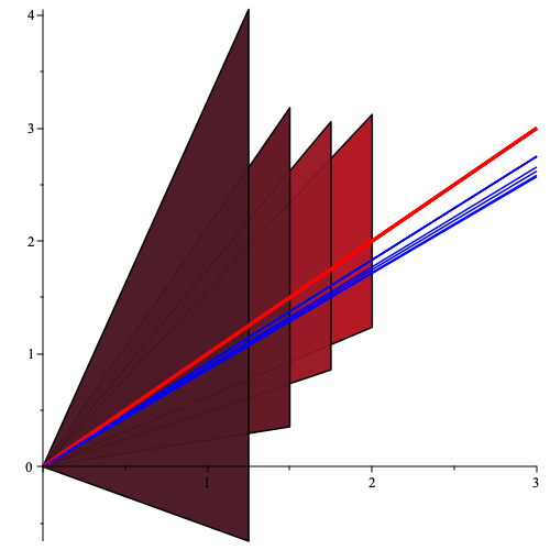
Figure 1. Cones $K_{n}$ for $n=1$ to $4$, where the color of $K_{n}$ becomes lighter for increasing $n$. The red vector is the limit of the cones, and the blue vectors represent $U_{0},\dots,U_{4}$.

It turns out that the sequence of contracted cones $(K_{n})_{n}$ also satisfies

$$A(n)K_{n}\subset K_{n+1},\quad\text{for all }n\geq N=3.$$

In other words, for $n\geq N$

$$U_{n}\in K_{n}\implies U_{n+1}=A(n)U_{n}\in K_{n+1}\in\mathbb{R}^{2}_{>0}.$$

As shown in Fig. 1, for $n=3$, $U_{3}\in K_{3}$. By induction, $U_{n}\in K_{n}\subset\mathbb{R}^{2}_{>0}$ for all $n\geq N=3$. Additionally, $U_{0},U_{1},U_{2}$ are in $\mathbb{R}^{2}_{>0}$, thus the sequence $(u_{n})_{n}$ is positive.

For this sequence, positivity is proved by constructing a sequence of contracted cones and induction. This approach extends to recurrences of Poincaré type where the recurrence operator $A(n)$ satisfies the contraction condition. More precisely, for $\lambda_{i,n}$ denoting the distinct eigenvalues of $A(n)$, we have

$$\lambda_{1,n}>|\lambda_{2,n}|\geq\dots\geq|\lambda_{k,n}|,\quad n\in\mathbb{N}$$

and $\lambda_{1,n}$ is simple. This approach is outlined in Algorithm 1.

Input: $A(n)$ companion matrix $\in\mathbb{Q}(n)^{d\times d}$ such that $A=\lim\limits_{n\to\infty}A(n)\in\mathbb{Q}^{d\times d}$; $A(n)$ satisfies the contraction condition (for $n$ large enough); $U_{0}\in\mathbb{Q}^{d}$

Output: Positivity of $(U_{n})_{n}$

1. Cone Construction: Compute $K_{n}\subset\mathbb{R}_{\geq 0}^{d}$ s.t. $A(n)(K_{n}\setminus\{0\})\subset K_{n}^{\circ}$.

2. Inclusion Index: Find $N\in\mathbb{N}$ s.t. for all $n\geq N$, $A(n)K_{n}\subset K_{n+1}$.

Initial Conditions Check: Compute $n_{0}\geq N$ s.t. $U_{n_{0}}\in K_{n_{0}}$, and check if $U_{0},U_{1},\dots,U_{n_{0}-1}$ are positive.

Algorithm 1 Main Steps of the Positivity Algorithm

The termination of this algorithm is studied by observing the asymptotic behavior of the eigenvalues $\lambda_{i,n}$ as $n\to\infty$.

4. Eigenvalues ordering

For a rational square matrix, the eigenvalues can be efficiently ordered by modulus using absolute separation bounds (BugeaudDujellaFangPejkovicSalvy2022, , Theorem 1). Let $A(n)$ be a matrix in $\mathbb{Q}(n)^{d\times d}$ with characteristic polynomial $P(n,X)$, and assume that

$$\lim_{n\to\infty}A(n)=A\in\mathbb{Q}^{d\times d}.$$

In the following, we show how the eigenvalues of $A(n)$, i.e. the roots of $P(n,X)$, can be ordered by modulus for sufficiently large $n$.

First, compute the polynomial $Q(Y,X)\in\mathbb{Q}[Y,X]$ the numerator of $P(1/Y,X)$. By construction, $Q(0,X)$ is the characteristic polynomial of $A$, up to a scalar.

By Puiseux theorem, the roots $X_{j}(Y)$ of $Q(Y,X)$ take the form

$$X_{j}(Y)=X_{j}+\sum_{k=1}^{\infty}c_{k}Y^{\frac{k}{m}},$$

where $X_{j}\in\mathbb{C}$ is a root of $P(0,X)$, $m$ is a positive integer and $c_{k}$ is in $\mathbb{C}$.

For sufficiently small $Y$, the number of roots $X_{j}(Y)$ with the same modulus remains constant. This allows us to define the sequence $(\rho_{i}(Y))_{i=1}^{\ell}$ representing the distinct modulus of the roots $X_{j}(Y)$. As $Y$ decreases to 0, we assume that $\rho_{i}(Y)$ have the following order

$$\rho_{1}(Y)>\rho_{2}(Y)>\dots>\rho_{\ell}(Y).$$

We denote by $q_{i}$ the number of roots with modulus $\rho_{i}(Y)$.

Remark 2.

If the $(q_{i})_{i=1}^{\ell}$ are known, the roots $X_{j}(Y)$ can be grouped by modulus using Puiseux expansions up to sufficient order.

Proposition 0.

For a square free bivariate polynomial $Q(Y,X)\in\mathbb{Q}[Y,X]$, Algorithm 2 computes $(q_{i})_{i=1}^{\ell}$.

Proof.

Algorithm 2 is an extension of algorithm 5 in(GourdonSalvy1996, ). For a square-free univariate polynomial, this algorithm computes iteratively the number of roots for each modulus, starting from the largest modulus to the smallest. The proof follows the same approach as in (GourdonSalvy1996, ). We sketch it for the computation of $q_{1}$.

For $Y$ decreasing to 0, the polynomial $Q_{Y}\otimes Q_{Y}\in\mathbb{Q}[Y,X]$ has $\rho_{1}(Y)^{2}$ as its unique dominant root. On the other hand, the polynomials $P_{i}$ are coprime. Thus, there exists a unique index $i_{0}$ such that $(\rho_{1}(Y))^{2}$ is a root of $P_{i_{0}}\in(\mathbb{Q}[Y])[X]$ and $q_{1}=i_{0}$.

To determine $i_{0}$, Algorithm 1 computes Puiseux expansions at 0 for the roots $\beta_{i,j}(Y)$, $i=1\dots\ell$. The uniqueness of $\rho_{1}(Y)^{2}$ as dominant root ensures that $\beta_{i_{0},j_{0}}(Y)$ is found using Puiseux expansions up to a finite order. This completes the proof. The computations of $Q_{Y}\otimes Q_{Y}$ and $\mathcal{P}_{m}$ can be done efficiently (GourdonSalvy1996, ). ∎

Input: $Q_{Y}(X)=\prod_{i=1}^{d}(X-X_{i}(Y))$ square free polynomial $\in\mathbb{Q}[Y][X]$ where $X_{i}=X_{i}(0)\in\mathbb{C}$.

Output: $q_{i}$: the number of roots of modulus $\rho_{i}(Y)$, as $Y$ decreases to 0.

1. Compute $Q_{Y}\otimes Q_{Y}=\prod_{i,j}(X-X_{i}(Y)X_{j}(Y))$.

2. Compute the square-free decomposition of $Q_{Y}\otimes Q_{Y}$ in the variable $X$:

   $$Q_{Y}\otimes Q_{Y}=P_{0}(Y)P_{1}(X,Y)P_{2}(X,Y)^{2}\dotsm P_{k}(X,Y)^{k}.$$

3. For each $i=1,\dots,k$, compute Puiseux expansions at $Y=0$ for the roots $\beta_{i,j}(Y)$ of the polynomial $P_{i}(X,Y)$,

4. Iteratively, increase the order of these expansions until finding $(i_{0},j_{0})$ such that $\beta_{i_{0},j_{0}}(Y)$ is a positive real root having the greatest modulus as $Y$ decreases to 0;

5. Set $q_{1}=i_{0}$.

6. Knowing $q_{i}$ for $i=1,\dots,j$, let $m=q_{1}+q_{2}+\dots+q_{j}+1$. Find $q_{j+1}$ by repeating the above steps for the polynomial

   $$\mathcal{P}_{m}(Y,X)=\prod_{i_{1}<i_{2}<\dots<i_{m}}\left(X-X_{i_{1}}(Y)X_{i_{2}}(Y)\dots X_{i_{m}}(Y)\right).$$

Algorithm 2 Number of Roots for each Modulus

5. Sequence of cones

For a matrix $A$ satisfying the contraction condition, Vandergraft’s construction of the cone is based on the eigenstructure of $A$. We first recall this construction and then show how to adapt it to define a sequence of cones $(K_{n})_{n}$ , each contracted by $A(n)$ .

5.1. Vandergraft’s Construction

We specialize Vandergraft’s construction to the case where $A$ is the companion matrix of the polynomial

$$P(X)=(X-\lambda_{1})(X-\lambda_{2})\cdots(X-\lambda_{\mu})(X-\lambda_{\mu+1})^{m_{\mu+1}}\cdots(X-\lambda_{k})^{m_{k}}.$$

Here, $\lambda_{i}$ denotes an eigenvalue of $A$, and $m_{i}$ is its multiplicity. The eigenvalues are assumed to satisfy

$$\lambda_{1}>|\lambda_{2}|\geq|\lambda_{3}|\geq\cdots\geq|\lambda_{\mu}|>|\lambda_{\mu+1}|\geq\cdots\geq|\lambda_{k}|,$$

and the first $\mu\geq 2$ of them are assumed to be simple.

5.1.1. Basis Construction

Fix $\varepsilon>0$ such that $|\lambda_{2}|-|\lambda_{\mu+1}|>\varepsilon$. If $\mu=\deg(P)$, take $\varepsilon=0$.

Construct a basis $(V_{i,j})$ of $\mathbb{R}^{d}$ satisfying the following properties:

(2) $$AV_{i,1} =\lambda_{i}V_{i,1}, 1\leq i\leq k,$$

$$AV_{i,j} =\lambda_{i}V_{i,j}+\varepsilon V_{i,j-1}, \mu+1\leq i\leq k,\ 2\leq j\leq m_{i}.$$

In other words, if $T$ is the matrix whose columns are the vectors
$(V_{i,j})_{j=1,\dots,m_{i},\ i=1,\dots,k}$, then

(3) $$T^{-1}AT=\begin{bmatrix}\lambda_{1}&\cdots&0&0&\cdots&0\\ \vdots&\ddots&\vdots&\vdots&\ddots&\vdots\\ 0&\cdots&\lambda_{\mu}&0&\cdots&0\\ 0&\cdots&0&J_{\varepsilon,\mu+1}&\cdots&0\\ \vdots&\ddots&\vdots&\vdots&\ddots&0\\ 0&\cdots&0&0&\cdots&J_{\varepsilon,k}\end{bmatrix}$$

with $J_{i,\varepsilon}$ the Jordan block

$$\qquad J_{i,\varepsilon}=\begin{bmatrix}\lambda_{i}&\varepsilon&0&\cdots&0\\ 0&\lambda_{i}&\varepsilon&\cdots&0\\ 0&0&\lambda_{i}&\ddots&\vdots\\ \vdots&\vdots&\ddots&\ddots&\varepsilon\\ 0&0&\cdots&0&\lambda_{i}\end{bmatrix}\in\mathbb{C}^{m_{i}\times m_{i}}.$$

Let $C$ be the set defined by

$$C=\Bigl{\{}\alpha=(\alpha_{1,1},\dots,\alpha_{j,m_{k}})\in\mathbb{C}^{d\times d}\Big{|} ~\alpha_{1,1}\geq|\alpha_{i,j}|,$$

$$\alpha_{i,j}=\overline{\alpha_{p,q}}\text{ if }V_{i,j}=\overline{V_{p,q}}, ~\alpha_{i,j}\in\mathbb{R}\text{ otherwise}\Bigr{\}}.$$

Then,

$$K=K(V_{i,j})=\{T\alpha|\alpha\in C\},$$

is a proper real cone contracted by $A$. This is proved along with Proposition 1 below.

For a vector $\beta=(\beta_{1},\dots,\beta_{d})$ in $\mathbb{C}^{d\times d}$, we use the norm

$$\|\beta\|=\max_{i=1}^{d}|\beta_{i}|.$$

$\Delta$ denotes the metric induced by the norm $\|\cdot\|$.

Proposition 0.

Let $S_{1}\subset K$ be the compact set defined by

$$S_{1}:=\{T\alpha|\alpha\in C\text{ and }\alpha_{1,1}=1\}.$$

Then, the distance between $T^{-1}AS_{1}$ and $T^{-1}\partial K$, where $\partial K$ denotes the boundary of $K$, satisfies:

$$\Delta(T^{-1}AS_{1},T^{-1}\partial K)\geq\frac{\lambda_{1}-|\lambda_{2}|}{2}>0.$$

Proof.

1. Action of $A$: Let $W=T\beta$ be a vector in $S_{1}$. By definition, $\beta_{1,1}=1$ and $|\beta_{i,j}|\leq 1$ for all $i,j$. In view of Eq. 3, $AW=T(T^{-1}AT)\beta=T\alpha$, where:

$$\alpha_{1,1}=\lambda_{1},$$

and for $i\neq 1$:

$$\alpha_{i,j}=\begin{cases}\beta_{i,j}\lambda_{i},&j=m_{i},\\ \beta_{i,j}\lambda_{i}+\varepsilon\beta_{i,j+1},&i\geq\mu+1,~j<m_{i}.\end{cases}$$

2. Bounding $|\alpha_{i,j}|$: Since $|\beta_{i,j}|\leq 1$, for $i\neq 1$ and $j=m_{i}$,

$$|\alpha_{i,j}|\leq|\lambda_{i}|\leq|\lambda_{2}|$$

For $i\geq\mu+1$ and $j<m_{i}$,

$$|\beta_{i,j}|\leq|\lambda_{i}|+|\varepsilon\beta_{i,j+1}|\leq|\lambda_{\mu+1}|+\varepsilon\leq|\lambda_{2}|.$$

Thus,

$$(AS_{1})\subset S_{2}:=\{T\alpha\mid\alpha_{1,1}=\lambda_{1},|\alpha_{i,j}|\leq|\lambda_{2}|\}.$$

By definition, $S_{2}$ is in the interior of $K$ and thus $K$ is contracted by$~A$.
3. Compactness of $AS_{1}$: $AS_{1}$ is a compact subset of $K^{\circ}$ because it is the image of a compact set $S_{1}$ under $A$.
4. Characterization of $\partial K$: A vector $T\alpha$ lies on the boundary of $K$ if and only if $\alpha_{1,1}=\displaystyle\max_{(i,j)\neq(1,1)}|\alpha_{i,j}|$, i.e.,

$$\partial K=\Bigl{\{}T\alpha\Big{|}~\alpha\in C,\alpha_{1,1}=\max_{(i,j)\neq(1,1)}|\alpha_{i,j}|\Bigr{\}}.$$

5. Distance Calculation: The inclusion in $S_{2}$ implies

$$\Delta(T^{-1}AS_{1},T^{-1}\partial K)\geq\Delta(T^{-1}S_{2},T^{-1}\partial{K})=\Delta(C_{1},C_{2})$$

where

$$C_{1} =\{\alpha\in C|~\alpha_{1,1}=\lambda_{1},|\alpha_{i,j}|\leq\lambda_{2}\},$$

$$C_{2} =\{\beta\in C|~\max_{i\neq 1}|\beta_{i,j}|=\beta_{1,1}\}.$$

By definition,

$$\Delta(C_{1},C_{2})=\min_{\alpha\in C_{1},~\beta\in C_{2}}\Delta(\alpha,\beta).$$

Let $(i_{0},j_{0})$ be the index such that $|\beta_{i_{0},j_{0}}|=|\beta_{1,1}|$; we have

$$\Delta(\alpha,\beta)\geq\max\Bigl{\{}|\lambda_{1}-\beta_{1,1}|,|\alpha_{i_{0},j_{0}}-\beta_{i_{0},j_{0}}|\Bigr{\}}.$$

For $|\beta_{1,1}|\leq\lambda_{1}$ or $|\beta_{1,1}|\leq|\lambda_{2}|$, by the inequality above we get

$$\Delta(\alpha,\beta)\geq\lambda_{1}-|\lambda_{2}|.$$

Now, for $|\lambda_{2}|\leq|\beta_{1,1}|\leq\lambda_{1}$,

$$|\lambda_{1}-\beta_{1,1}| =\lambda_{1}-|\beta_{1,1}|$$

$$|\alpha_{i_{0},j_{0}}-\beta_{i_{0},j_{0}}| \geq|\beta_{i_{0},j_{0}}|-|\alpha_{i_{0},j_{0}}|\geq|\beta_{1,1}|-|\lambda_{2}|.$$

Combining all these bounds, we get

$$\Delta(\alpha,\beta)\geq\max_{|\lambda_{2}|\leq|\beta_{1,1}|\leq\lambda_{1,1}}\Bigl{\{}\lambda_{1}-|\beta_{1,1}|,|\beta_{1,1}|-|\lambda_{2}|\Bigr{\}}\geq\frac{\lambda_{1}-|\lambda_{2}|}{2}.$$

Then, $\Delta(C_{1},C_{2})\geq\frac{\lambda_{1}-|\lambda_{2}|}{2}$. This completes the proof. ∎

5.2. Construction of a sequence of contracted cones

Let $A(n)\in\mathbb{Q}(n)^{d\times d}$ be the companion matrix of the polynomial

$$P(n,X)=(X-\lambda_{1,n})\cdots(X-\lambda_{v,n})(X-\lambda_{v+1,n})^{m_{v+1}}\cdots(X-\lambda_{k,n})^{m_{k}},$$

where $\lambda_{i,n}\in\mathbb{C}$ are the eigenvalues of $A_{n}$, with multiplicities $m_{i}$ (we can assume that $m_{i}$ is constant for sufficiently large $n$).
$A(n)$ is assumed to satisfy the contraction condition, i.e. ,

$$\lambda_{1,n}>|\lambda_{2,n}|\geq\dots\geq|\lambda_{v,n}|>|\lambda_{v+1,n}|\geq|\lambda_{v+2,n}|\dots\geq|\lambda_{k,n}|.$$

The ordering is done as shown in Section 4

Basis vectors

First, we can fix $\varepsilon>0$, independent of $n$, such that $0<\varepsilon<|\lambda_{2,n}|-|\lambda_{v+1,n}|$ for $n$ large enough. For this choice of $\varepsilon$, the vectors $\{V_{i,j}(n)\}$ below are solutions of Eq. 2:

(4) $$V_{1,1}(n) =d(1,\lambda_{1,n},\dots,\lambda_{1,n}^{d-1})$$

$$V_{i,1}(n) =(1,\lambda_{i,n},\dots,\lambda_{i,n}^{d-1}),\quad 1\leq i\leq k.$$

For $\mu+1\leq i\leq k,~2\leq j\leq m_{i}$,

$$V_{i,j}(n)=\varepsilon^{j-1}\left(\binom{\ell}{j-1}\lambda_{i,n}^{\ell-j+1},\ell=0,\dots,d-1\right).$$

If $\lambda_{i,n}=0$, then take

$$V_{i,j}(n)=\varepsilon^{j-1}(0,\dots,0,1,0,\dots,0),$$

with 1 in the $j$th position.

Proposition 0.

For $n$ large enough, the cone $K_{n}=K(V_{i,j}(n))$ is positive.

Proof.

For simplicity, we denote $V_{i,j}=V_{i,j}(n)$ in this proof. Let $W$ be a vector in $K(V_{i,j})$. Up to scaling, we can assume that

$$W=V_{1,1}+\sum_{i\neq 1}\alpha_{i,j}V_{i,j},\quad|\alpha_{i,j}|\leq 1.$$

For a vector $x\in\mathbb{C}^{d}$, we denote by $(x)_{l}$ the $(l+1)$-th coordinate of the vector. For $\ell=0,\dots,d-1$, we have

$$(W)_{\ell} =(V_{1,1})_{\ell}+\sum_{i\neq 1}\sum_{j=1}^{m_{i}}\alpha_{i,j}(V_{i,j})_{\ell}$$

$$\geq d\lambda_{1}^{\ell}-\sum_{i\neq 1}\sum_{j=1}^{m_{i}}|\alpha_{i,j}(V_{i,j})_{\ell}|$$

$$\geq d\lambda_{1}^{\ell}-\sum_{i\neq 1}\sum_{j=1}^{m_{i}}|(V_{i,j})_{\ell}|.$$

Now, for any fixed $i\neq 1$, we prove that

$$\sum_{j=1}^{m_{i}}|(V_{i,j})_{\ell}|\leq\lambda_{1}^{\ell}.$$

By definition of the vectors $V_{i,j}$, we have

$$\sum_{j=1}^{m_{i}}|(V_{i,j})_{\ell}| =\sum_{j=1}^{m_{i}}\varepsilon^{j-1}\binom{\ell}{j-1}|\lambda_{i}|^{\ell-j+1}$$

$$\leq(|\lambda_{i}|+\varepsilon)^{\ell}<|\lambda_{1}|^{\ell}.$$

Thus, we have shown that $(W)_{\ell}>0$ for all $\ell=0,\dots,d-1$, which implies that $W\in\mathbb{R}^{d}_{>0}$. Therefore, the cone $K_{n}$ is positive. ∎

6. Several Simple Dominant Eigenvalues

For recurrences having several dominant eigenvalues, all simple, we now give asymptotic condition on the eigenvalues of $A(n)$, ensuring the existence of a sequence of contracted cones $(K_{n})_{n}$ such that $A(n)K_{n}\subset K_{n+1}$ for $n$ large enough.

Theorem 1.

Let $A(n)\in\mathbb{Q}(n)^{d\times d}$ be the companion matrix of the polynomial

$$P(n,X)=(X-\lambda_{1,n})\cdots(X-\lambda_{v,n})(X-\lambda_{v+1,n})^{m_{v+1}}\cdots(X-\lambda_{k,n})^{m_{k}},$$

where $\lambda_{i,n}\in\mathbb{C}$ are the eigenvalues of $A_{n}$, with multiplicities $m_{i}$.

Assume that the following conditions hold:

1. Contraction condition: $\lambda_{1,n}\geq|\lambda_{i,n}|$ for all $i\neq 1$ and $n$ sufficiently large.

2. The eigenvalues $\lambda_{i,n}$ converge as $n\to\infty$ to distinct limits $\lambda_{i}\in\mathbb{C}$, satisfying:

   $$\lambda_{1}=|\lambda_{2}|=\cdots=|\lambda_{v}|>|\lambda_{j}|\quad\text{for }j>v.$$

3. $\underset{i=1,\dots,k}{\max}|\lambda_{i,n}-\lambda_{i,n+1}|=o\left(\lambda_{1,n}-\underset{j=2,\dots,v}{\max}|\lambda_{j,n}|\right),~n\to\infty.$

Then, there exists a sequence of proper positive cones $K_{n}\subset\mathbb{R}^{d}$ such that $A_{n}K_{n}\subseteq K_{n+1}$, for sufficiently large $n$.

Proof.

When $v=1$, the limit matrix $A$ of $A(n)$ satisfies the contraction condition. In this case, we can take $K_{n}=K$, where $K$ is the cone contracted by $A$, as shown in (ibrahim2024positivityproofslinearrecurrences, ).

We know focus on the case $v>1$. For a fixed $n$, $A(n)$ satisfies condition (1). By Theorem 3, $A(n)$ contracts a proper cone $K_{n}$. We take $K_{n}$ specifically as $K_{n}=K(V_{i,j}(n))\subset\mathbb{R}^{d}_{>0}$, defined in Section 5.1.1.

For $n\in\mathbb{N}$, $T_{n}$ denotes the matrix having for columns the vectors $V_{i,j}(n)$. In the following, we prove that $A(n)K_{n}\subset K_{n+1}$.

Since $K_{n}$ is a cone, by linearity, it suffices to show that the inclusion holds for the vectors in $S_{1}(K_{n})$, where

$$S_{1}(K_{n})=\{W=T_{n}\alpha\mid\alpha\in C,~\alpha_{1,1}=1\}.$$

Let $W_{n}=T_{n}\alpha$ be a vector in $S_{1}(K_{n})$. Then $W_{n+1}=T_{n+1}\alpha$ is a vector in $S_{1}(K_{n+1})$, and its image $A(n+1)W_{n+1}$ lies in the interior of $K_{n+1}$.

We introduce the norm

$$\|x\|_{n}=\|T_{n}^{-1}x\|,$$

and $\Delta_{n}$ the distance induced by $\|.\|_{n}$. As shown by Proposition 1,

$$\Delta_{n+1}(A(n+1)W_{n+1},\partial K_{n+1})\geq\frac{\lambda_{1,n+1}-|\lambda_{2,n+1}|}{2}.$$

To prove the inclusion property, it is sufficient to show that

$$\|A(n)W_{n}-A(n+1)W_{n+1}\|_{n+1}<\frac{\lambda_{1,n+1}-|\lambda_{2,n+1}|}{2}.$$

This ensures that $A(n)W_{n}$ is contained in $K_{n+1}$.

By definition, we have

$$\|A(n)W_{n}-A(n+1)W_{n+1}\|_{n+1} =\|(A(n)T_{n}-A(n+1)T_{n+1})\alpha\|_{n+1}$$

$$=\|T_{n+1}^{-1}(A(n)T_{n}-A(n+1)T_{n+1})\alpha\|$$

$$\leq\|T_{n+1}^{-1}(A(n)T_{n}-A(n+1)T_{n+1})\|$$

since $\|\alpha\|=1$. Next, we use the following relation for $T_{n+1}^{-1}$,

$$T_{n+1}^{-1}-T_{n}^{-1}=T_{n+1}^{-1}(T_{n}-T_{n+1})T_{n}^{-1}.$$

This leads to the inequality,

$$\|A(n)W_{n}-A(n+1) W_{n+1}\|_{n+1}\leq\|T_{n}^{-1}A(n)T_{n}-T_{n+1}^{-1}A(n+1)T_{n+1}\|$$

$$\quad+\|T_{n+1}^{-1}(T_{n}-T_{n+1})T_{n}^{-1}A(n)T_{n}\|.$$

Since

$$T_{n}^{-1}A(n)T_{n}=\begin{bmatrix}\lambda_{1,n}&0&\cdots&0\\ 0&\lambda_{2,n}&\cdots&0\\ \vdots&\vdots&\ddots&\vdots\\ 0&0&\cdots&J_{k_{n},\varepsilon}\end{bmatrix},$$

we obtain first the following bound as $n\to\infty$,

(5) $$\|T_{n}^{-1}A(n)T_{n}-T_{n+1}^{-1}A(n+1)T_{n+1}\|=O\left(\max_{i=1,\dots,k}|\lambda_{i,n}-\lambda_{i,n+1}|\right).$$

Next, let $(t_{i,j})$ denote the entries of $T_{n+1}-T_{n}$. Then, by Eq. 2,

$$t_{i,j}=c_{i,j}(\lambda_{i,n}^{j-1}-\lambda_{i,n+1}^{j-1}),\quad n\to\infty$$

where $c_{i,j}$ are constants independent of $n$. Therefore, the norm of the difference $T_{n+1}-T_{n}$ can be bounded as

$$\|T_{n+1}-T_{n}\|=O\left(\max_{i=1,\dots,k}|\lambda_{i,n}-\lambda_{i,n+1}|\right),~n\to\infty.$$

Due to the dominance of $\lambda_{1,n}$ and the condition on $\varepsilon$,

(6) $$\|T_{n}^{-1}A(n)T_{n}\|=\lambda_{1,n}\to\lambda_{1},\quad n\to\infty.$$

Since $T_{n}\to T$ (invertible by condition (2)), $\|T_{n+1}^{-1}\|$ is bounded as $n$ tends to infinity. Combining this with the bound in Eq. 6,

(7) $$\|T_{n+1}^{-1}(T_{n}-T_{n+1})T_{n}^{-1}A(n)T_{n}\|=O\left(\max_{i=1,\dots,k}|\lambda_{i,n}-\lambda_{i,n+1}|\right).$$

Finally, by Eq. 7 and Eq. 5, as $n\to\infty$

$$\|A(n)W_{n}-A(n+1)W_{n+1}\|_{n+1}=O\left(\max_{i=1,\dots,k}|\lambda_{i,n}-\lambda_{i,n+1}|\right),$$

which is smaller than $\frac{\lambda_{1,n+1}-|\lambda_{2,n+1}|}{2}$ asymptotically. Indeed, condition (3), asserts

$$\underset{i=1,\dots,k}{\max}|\lambda_{i,n}-\lambda_{i,n+1}|=o(\lambda_{1,n}-|\lambda_{2,n}|),\quad n\to\infty.$$

Under this assumption, we prove that

(8) $$\lambda_{1,n+1}-|\lambda_{2,n+1}|\sim\lambda_{1,n}-|\lambda_{2,n}|,\quad n\to\infty.$$

Consequently, as $n\to\infty$

$$\underset{i=1,\dots,k}{\max}|\lambda_{i,n}-\lambda_{i,n+1}|=o(\lambda_{1,n+1}-|\lambda_{2,n+1}|),$$

thus $A_{n}K_{n}\subseteq K_{n+1}$ for $n$ large enough.

In fact,

$$|\lambda_{1,n+1}-\lambda_{1,n}| =O\Bigl{(}\underset{i=1,\dots,k}{\max}|\lambda_{i,n}-\lambda_{i,n+1}|\Bigr{)}$$

$$||\lambda_{2,n}|-|\lambda_{2,n+1}|| \leq|\lambda_{2,n}-\lambda_{2,n+1}|=O\Bigl{(}\underset{i=1,\dots,k}{\max}|\lambda_{i,n}-\lambda_{i,n+1}|\Bigr{)}.$$

Then,

$$\lambda_{1,n+1}-|\lambda_{2,n+1}|=\lambda_{1,n}-|\lambda_{2,n}|+O(\underset{i=1,\dots,k}{\max}|\lambda_{i,n}-\lambda_{i,n+1}|).$$

Thus, by condition (3) we obtain the equivalence in Eq. 8. ∎

Proposition 0.

Let $(u_{n})_{n}$ be a P-finite sequence satisfying the recurrence in Eq. 1, of Poincaré type. Assume that:

• The recurrence has several dominant eigenvalues, all simple.

• One of these eigenvalues, denoted $\lambda_{1}$, is real and positive.

• The associated operator $A(n)$ satisfies the conditions of Theorem 1.

• $V_{1}$ is a positive eigenvector of the limit matrix $A$ associated with $\lambda_{1}$ and

  $$\lim_{n\to\infty}\frac{U_{n}}{\|U_{n}\|}=V_{1}.$$

Then, the positivity of $(u_{n})_{n}$ is decidable.

Proof.

We prove the termination of Algorithm 1 under these conditions.

Take $K_{n}=K(V_{i,j}(n))\subset\mathbb{R}^{d}_{>0}$. By Theorem 1, there exists $N\in\mathbb{N}$ such that

$$A(n)K_{n}\subset K_{n+1},\quad\forall n\geq N.$$

Thus, termination depends on verifying the initial conditions, i.e., proving that $U_{n}\in K_{n}$ for sufficiently large $n$.

First, the vector $V_{1}$ and $\lim\limits_{n\to\infty}V_{1,1}(n)$ are both positive eigenvectors of $A$ associated with $\lambda_{1}$. Thus, there exists a constant $\beta>0$ such that

$$\lim\limits_{n\to\infty}V_{1,1}(n)=\beta~V_{1}.$$

Since $V_{1,1}(n)$ is in the interior of $K_{n}$, we compute its distance to the boundary $\partial K_{n}$ that remains strictly positive:

$$\Delta_{n}(V_{1,n},\partial K_{n})=\Delta(T_{n}^{-1}V_{1,n},T_{n}^{-1}\partial K_{n})=\Delta((1,0,\dots,0),C_{2}),$$

where $C_{2}=T_{n}^{-1}\partial K_{n}$ is defined in Section 5.1.1. Using the same approach in the proof of Proposition 1, we get

$$\Delta((1,0,\dots,0),C_{2})=\frac{1}{2}.$$

On the other hand, let $W_{n}=\beta~U_{n}/\|U_{n}\|$. Then,

$$\|V_{1,1}(n)-W_{n}\|_{n}\leq\|T_{n}^{-1}\|(\|V_{1,1}(n)-\beta V_{1}\|+\|\beta V_{1}-W_{n}\|).$$

Since $\|T_{n}^{-1}\|$ is bounded, $\|V_{1,1}(n)-W_{n}\|_{n}$ becomes arbitrarily small as $n\to\infty$. Thus, for $n$ sufficiently large, $U_{n}$ remains in the cone $K_{n}$.

Returning to Algorithm 1, once we find $n_{0}\in\mathbb{N}$ such that $U_{n_{0}}\in K_{n_{0}}$, by induction $U_{n}$ remains in $K_{n}\subset\mathbb{R}^{d}_{>0}$ for all $n\geq n_{0}$. Therefore, deciding positivity reduces to checking the sign of the initial values $U_{0},\dots,U_{n_{0}-1}$. ∎

7. Examples

We now present examples for which the positivity could not be proven using our previous algorithm.

• For $x\in(0,1)$, consider the inequality:

$$f(x)={}_{2}F_{1}\left(\frac{1}{2},\frac{1}{2};1;x^{2}\right)-(1+x)\,{}_{2}F_{1}\left(\frac{1}{2},\frac{1}{2};1;x\right)\geq 0.$$

Let $(a_{n})_{n}$ be the sequence of coefficients in the Taylor expansion of $f(x)$, i.e., $f(x)=\sum_{n=0}^{\infty}a_{n}x^{n}$. By closure properties, $(a_{n})_{n}$ is a P-finite sequence and satisfies a recurrence of order 6. If both sequences $(u_{n})_{n}$ and $(w_{n})_{n}$, defined by $w_{n}=a_{2n+1}$ and $u_{n}=a_{2n}$, are positive, then the inequality is proven. The sequence $(w_{n})_{n}$ satisfies the recurrence:

$$64(32n^{2}+24n+5) (2n+3)^{2}(n+1)^{2}w_{n+1}=$$

$$(32n^{2}+88n+61)(4n+3)^{2}(4n+1)^{2}w_{n}.$$

Thus, positivity is trivial.

On the other hand, $(u_{n})_{n}$ is the solution of a second-order recurrence relation with a double eigenvalue $\lambda_{1}=1$. However, the matrices $A(n)$ satisfy the contraction condition. Applying Algorithm 1, the vectors $U(n)=(u_{n},u_{n+1})\in K_{n}\subset\mathbb{R}^{2}_{>0}$ for all $n\geq 2$. Thus, $(u_{n})_{n}$ is positive.

• Let $P_{k}$ denote the $k$-th Legendre polynomial. The following example is Turàn’s inequality for $x=\frac{1}{2}$,

$$(P_{n}^{2}-P_{n-1}P_{n+1})(\frac{1}{2})\geq 0,\quad n\in\mathbb{N}.$$

The associated sequence $(u_{n})_{n}$ satisfies a recurrence of order $3$ and its characteristic polynomial is $X^{3}-1$. However, as $n\to\infty$

$$\lambda_{1,n}\sim 1-\frac{1}{n},~\lambda_{2,n}\sim\frac{-1+i\sqrt{3}}{2}+\frac{3(1-i\sqrt{3})}{2n},~\lambda_{3,n}=\overline{\lambda_{2,n}}.$$

Thus, the conditions of Proposition 2 are satisfied and by Algorithm 1 the vectors $U_{n}\in K_{n}\subset\mathbb{R}^{3}_{>0}$ for all $n\geq 8$.

Remark 3.

The above inequality holds for all $-1\leq x\leq 1$ . Using Algorithm 1 to prove it, we observe that the inclusion index $N\to\infty$ as $x$ approaches the boundary points $-1$ and $1$.

8. Approximations by Asymptotic Truncation

In practice, computing the cone $K_{n}$ in Algorithm 1 is simplified by approximating the eigenvalues $\lambda_{i,n}$ through asymptotic expansions. Specifically, we truncate the expansions of $\lambda_{i,n}$ as $n\to\infty$. The order of truncation is iteratively increased if necessary.

For instance, in Section 3, the cone $K_{n}$ was constructed by taking an asymptotic truncation of $\lambda_{i,n}$ up to order $1$:

$$\lambda_{1,n}\sim 1+\frac{-2+\sqrt{2}}{n},~\lambda_{2,n}\sim 1-\frac{2+\sqrt{2}}{n},\quad n\to\infty.$$

With these approximations, we construct the associated vectors $V_{i,j}(n)$, and then the cone $K_{n}$ is given by

$$K_{n}=K({V_{i,j}(n)}),\quad n>0.$$

Remark 4.

The computations for the steps following the construction of the sequence of cones can be carried out as outlined in (ibrahim2024positivityproofslinearrecurrences, , section 6 ).

9. Conclusion

We present a method for proving positivity of P-finite sequences of Poincaré type under the assumption that the associated recurrence operator satisfies the contraction condition. This extends the approach in (ibrahim2024positivityproofslinearrecurrences, ) to a larger class of recurrences, where the dominant eigenvalue is not necessarily unique or simple.

For recurrences with multiple simple dominant eigenvalues of arbitrary order, we give an asymptotic conditions on the eigenvalues of the recurrence operator that ensure the existence of a sequence of cones, each mapped into the next by the recurrence operator. Under an assumption on the asymptotic behavior of the sequence, this allows us to decide positivity within this class of recurrences. This assumption depends on the choice of initial conditions and is analogous to the genericity assumption in (ibrahim2024positivityproofslinearrecurrences, ; KauersPillwein2010a, ). Moreover, under this assumption the termination of the method can be detected in advance by checking whether the asymptotic conditions on the eigenvalues are satisfied. This is the main distinction with the Gerhold-kauers method (GerholdKauers2005, ).

In other works, analytic techniques were used to prove positivity (MelczerMezzarobba2022, ; BostanYurkevich2022a, ). Our approach, instead, relies on algebraic tools, as we aim to generalize the cone-based method to recurrences with real parameters.

References

- [1] G. D. Anderson, R. W. Barnard, K. C. Richards, M. K. Vamanamurthy, and M. Vuorinen. Inequalities for zero-balanced hypergeometric functions. Transactions of the American Mathematical Society, 347(5):1713–1723, 1995.
- [2] S. Boldo, F. Clément, J.-C. Filliâtre, M. Mayero, G. Melquiond, and P. Weis. Trusting computations: a mechanized proof from partial differential equations to actual program. Comput. Math. Appl., 68(3):325–352, 2014.
- [3] A. Bostan and S. Yurkevich. A hypergeometric proof that iso is bijective. Proc. Amer. Math. Soc., 150(5):2131–2136, 2022.
- [4] Y. Bugeaud, A. Dujella, W. Fang, T. Pejković, and B. Salvy. Absolute root separation. Experimental Mathematics, 31(3):805–812, 2022.
- [5] G. E. Collins. Quantifier elimination for real closed fields by cylindrical algebraic decompostion. In Automata Theory and Formal Languages: 2nd GI Conference Kaiserslautern, May 20–23, 1975, pages 134–183. Springer, 1975.
- [6] S. Gerhold and M. Kauers. A procedure for proving special function inequalities involving a discrete parameter. Proceedings of the 2005 international symposium on Symbolic and algebraic computation - ISSAC ’05, 2005.
- [7] S. Gerhold and M. Kauers. A computer proof of Turán’s inequality. Journal of Inequalities in Pure and Applied Mathematics, 7(2):Article 42, 2006.
- [8] X. Gourdon and B. Salvy. Effective asymptotics of linear recurrences with rational coefficients. Discrete Mathematics, 153(1–3):145–163, 1996.
- [9] A. Humenberger, M. Jaroschek, and L. Kovács. Automated generation of non-linear loop invariants utilizing hypergeometric sequences. In ISSAC’17—Proceedings of the 2017 ACM International Symposium on Symbolic and Algebraic Computation, pages 221–228. ACM, New York, 2017.
- [10] A. Humenberger, M. Jaroschek, and L. Kovács. Invariant generation for multi-path loops with polynomial assignments. In Verification, model checking, and abstract interpretation, volume 10747 of Lecture Notes in Comput. Sci., pages 226–246. Springer, Cham, 2018.
- [11] A. Ibrahim and B. Salvy. Positivity certificates for linear recurrences. In Proceedings of the 2024 ACM-SIAM Symposium on Discrete Algorithms, SODA 2024, Alexandria, VA, USA, January 7-10, 2024, pages 982–994. SIAM, 2024.
- [12] A. Ibrahim and B. Salvy. Positivity proofs for linear recurrences through contracted cones, 2024. arXiv:2412.08576.
- [13] M. Kauers. Computer algebra and power series with positive coefficients. In Formal Power Series and Algebraic Combinatorics, Tianjin, China, 2007.
- [14] M. Kauers and V. Pillwein. When can we detect that a P-finite sequence is positive? In ISSAC 2010—Proceedings of the 2010 International Symposium on Symbolic and Algebraic Computation, pages 195–201. ACM, New York, 2010.
- [15] G. Kenison, O. Klurman, E. Lefaucheux, F. Luca, P. Moree, J. Ouaknine, M. A. Whiteland, and J. Worrell. On positivity and minimality for second-order holonomic sequences. In 46th International Symposium on Mathematical Foundations of Computer Science, volume 202 of LIPIcs. Leibniz Int. Proc. Inform., pages Art. No. 67, 15. Schloss Dagstuhl. Leibniz-Zent. Inform., Wadern, 2021.
- [16] G. Kenison, J. Nieuwveld, J. Ouaknine, and J. Worrell. Positivity Problems for Reversible Linear Recurrence Sequences. In K. Etessami, U. Feige, and G. Puppis, editors, 50th International Colloquium on Automata, Languages, and Programming (ICALP 2023), volume 261 of Leibniz International Proceedings in Informatics (LIPIcs), pages 130:1–130:17, Dagstuhl, Germany, 2023. Schloss Dagstuhl – Leibniz-Zentrum für Informatik.
- [17] S. Melczer and M. Mezzarobba. Sequence positivity through numeric analytic continuation: uniqueness of the Canham model for biomembranes. Comb. Theory, 2(2):Paper No. 4, 20, 2022.
- [18] M. Mezzarobba and B. Salvy. Effective bounds for P-recursive sequences. Journal of Symbolic Computation, 45(10):1075–1096, Oct. 2010.
- [19] D. S. Mitrinovic, E. Barnes, D. Marsh, and J. Radok. Elementary inequalities. Noordhoff Groningen, 1964.
- [20] J. Ouaknine and J. Worrell. On the positivity problem for simple linear recurrence sequences. In Automata, languages, and programming. Part II, volume 8573 of Lecture Notes in Comput. Sci., pages 318–329. Springer, Heidelberg, 2014.
- [21] J. Ouaknine and J. Worrell. Positivity problems for low-order linear recurrence sequences. In Proceedings of the Twenty-Fifth Annual ACM-SIAM Symposium on Discrete Algorithms, pages 366–379. ACM, New York, 2014.
- [22] V. Pillwein. Positivity of certain sums over Jacobi kernel polynomials. Advances in Applied Mathematics, 41(3):365–377, 2008.
- [23] V. Pillwein. Termination conditions for positivity proving procedures. In ISSAC 2013—Proceedings of the 38th International Symposium on Symbolic and Algebraic Computation, pages 315–321. ACM, New York, 2013.
- [24] A. D. Scott and A. D. Sokal. Complete monotonicity for inverse powers of some combinatorially defined polynomials. Acta Math., 213(2):323–392, 2014.
- [25] R. Serra, D. Arzelier, M. Joldes, J.-B. Lasserre, A. Rondepierre, and B. Salvy. Fast and accurate computation of orbital collision probability for short-term encounters. Journal of Guidance, Control, and Dynamics, 39(5):1009–1021, 2016.
- [26] R. P. Stanley. Enumerative combinatorics, volume 2. Cambridge University Press, 1999.
- [27] A. Straub and W. Zudilin. Positivity of rational functions and their diagonals. J. Approx. Theory, 195:57–69, 2015.
- [28] J. S. Vandergraft. Spectral properties of matrices which have invariant cones. SIAM J. Appl. Math., 16:1208–1222, 1968.
- [29] T. Yu and J. Chen. Uniqueness of Clifford torus with prescribed isoperimetric ratio. Proc. Amer. Math. Soc., 150(4):1749–1765, 2022.