SN 2023ixf in the Pinwheel Galaxy M101: From Shock Breakout to the Nebular Phase
Abstract
We present photometric and spectroscopic observations of SN 2023ixf covering from day one to 442 days after explosion. SN 2023ixf reached a peak -band absolute magnitude of , and light curves show that it is in the fast-decliner (IIL) subclass with a relatively short “plateau” phase (fewer than days). Early-time spectra of SN 2023ixf exhibit strong, very narrow emission lines from ionized circumstellar matter (CSM), possibly indicating a Type IIn classification. But these flash/shock-ionization emission features faded after the first week and the spectrum evolved in a manner similar to that of typical Type II SNe, unlike the case of most genuine SNe IIn in which the ejecta interact with CSM for an extended period of time and develop intermediate-width emission lines. We compare observed spectra of SN 2023ixf with various model spectra to understand the physics behind SN 2023ixf. Our nebular spectra (between 200-400 d) match best with the model spectra from a 15 progenitor which experienced enhanced mass loss a few years before explosion. A last-stage mass-loss rate of from the r1w6 model matches best with the early-time spectra, higher than derived from the ionized H luminosity at 1.58 d. We also use SN 2023ixf as a distance indicator and fit the light curves to derive the Hubble constant by adding SN 2023ixf to the existing sample; we obtain H km s-1 Mpc-1, consistent with the results from SNe Ia and many other independent methods.
fixltx2e
,
,
,
1 Introduction
Type II supernovae (hereafter SNe II) are characterized by strong hydrogen Balmer lines in their optical spectra (e.g., Filippenko, 1997). Thanks to progenitor detections (e.g., Van Dyk et al., 2003; Smartt, 2009, 2015; Van Dyk, 2017), it is commonly accepted that SNe II are massive-star explosions at the end of their lives (). While historically, SNe II were subgrouped based on their light-curve mythologies as SNe IIP with a long-duration plateau and SNe IIL with faster linear decline rates in magnitude, recent studies suggest that the light curves actually form a more continuous distribution (e.g., Anderson et al., 2014; Sanders et al., 2015; Valenti et al., 2016; Galbany et al., 2016; de Jaeger et al., 2019).
However, even if SNe II constitute a uniform physical family, a great variety of objects is seen in terms of their photometric and spectroscopic properties. This diversity results from differences among progenitors and explosion mechanisms (e.g., mass of hydrogen envelope, radius, metallicity). For example, SNe II whose optical spectra exhibit long-lasting, intermediate-width emission lines that indicate expansion speeds of a few hundred to km s-1, but little or no P Cygni absorption component, have been dubbed SNe IIn by Schlegel (1990); the “n” indicates the presence of the relatively “narrow” component. Examples were studied by Filippenko (1989, 1991a, 1991b), Stathakis & Sadler (1991), and others thereafter. The SN ejecta in these objects are likely interacting with circumstellar matter (CSM). However, Ransome et al. (2021) examine a wide variety of objects proposed to be SNe IIn, concluding that many of them do not even actually correspond to the terminal explosions of stars and are thus “SN impostors,” a term coined by Van Dyk et al. (2000) and subsequently used by many other authors.
In some cases, SNe IIn also show very narrow emission lines from gas having speeds km s-1; these are probably produced by flash or photoionization of CSM soon after shock breakout. Well-known examples include (among many others) SN 1998S (Leonard et al., 2000), SN 2013fs (Yaron et al., 2017), SN 2013cu (Gal-Yam et al., 2014), SN 2014G (Terreran et al., 2016), SN 2017ahn (Tartaglia et al., 2021), SN 2020pni (Terreran et al., 2022), and SN 2020tlf (Jacobson-Galán et al., 2022). These very narrow emission lines often disappear within a few days or a week, and the SN thereafter evolves in a manner more similar to that of typical Type II SNe (Bruch et al., 2023; Jacobson-Galán et al., 2024a). Such objects, with only fleeting narrow emission lines and no long-lasting intermediate-width component, do not necessarily qualify as genuine SNe IIn, although opinions regarding this differ among authors.
Turning now to one aspect of their cosmological significance, SNe II have been established as useful independent extragalactic distance indicators (e.g., Hamuy & Pinto, 2002; de Jaeger et al., 2020), especially for determining the Hubble-Lemaître constant (see de Jaeger & Galbany 2023 for a review) and addressing the current tension between early- and late-Universe measurements (Riess et al., 2022).
Owing to its exceptionally early detection in a nearby galaxy, SN 2023ixf provides a unique opportunity to explore and understand the zoo of SNe II; photometry and spectra were acquired starting day after the explosion. Moreover, SN 2023ixf allows us to test the accuracy of different extragalactic distance methods found in the literature.
SN 2023ixf was discovered by Koichi Itagaki on 2023-05-19 at 17:27:15 (UTC dates are used throughout this paper) at a Clear-band magnitude of 14.9 (Itagaki, 2023), in the nearby galaxy Messier 101 (M101, also known as NGC 5457 and informally as the “Pinwheel Galaxy”). Since M101 is a famous face-on spiral galaxy, it is regularly imaged by amateur astronomers throughout the world. After Itagaki reported the discovery of SN 2023ixf, many groups including amateurs and professionals reported prediscovery detections (Perley & Irani, 2023; Filippenko et al., 2023; Fulton et al., 2023; Zhang et al., 2023b; Hamann, 2023; Limeburner, 2023; Mao et al., 2023; Yaron et al., 2023; Koltenbah, 2023; Chufarin et al., 2023); see, in particular, the early-time unfiltered light curve of Sgro et al. (2023) obtained with Unistellar 11.4 cm telescopes and the multiband photometry of Li et al. (2024). These prediscovery observations range from a few minutes to a few days before Itagaki’s first report, and cover well before and after the explosion time of SN 2023ixf; thus, the explosion time can be precisely estimated (Hosseinzadeh et al., 2023; Hiramatsu et al., 2023). In this paper, we adopt the first-light time of SN 2023ixf to be MJD = 60082.788 estimated by Li et al. (2024).
Besides SN 2023ixf, M101 also hosted a few other historical SNe, including SN 1909A (type unknown), SN 1951H (type unknown), SN 1970G (Type II), and SN 2011fe (Type Ia). Among these, the most important is SN Ia 2011fe since it is one of the best-observed SNe and can be used for precise distance () estimation. Vinkó et al. (2012) fit the multiband light curves of SN 2011fe using both the MLCS2k2 and SALT2 methods, deriving Mpc (distance modulus mag) from MLCS2k2 and Mpc ( mag) from SALT2.
Given the proximity of M101, there are many other methods for measuring its distance. The most common and reliable one uses Cepheid variables. Over the past quarter century, several groups have independently measured the distance to M101 using Cepheids (Freedman et al., 2001; Saha et al., 2006; Shappee & Stanek, 2011). Riess et al. (2022) reported the latest Cepheid distance of Mpc ( mag). The optical tip of the red giant branch (TRGB) method is another option for distance measurement; Beaton et al. (2019) found ( mag) using the latest TRGB method. Here for our absolute-magnitude analysis, we adopt mag from Riess et al. (2022).
This paper is organized as follows. Section 2 contains a description of the observations and the data. In Section 3, we discuss the evolution of the light curves and color curves, while in Section 4, we present the analysis of the spectroscopic data. Section 5 compares different methods to measure distances, and we conclude with a summary in Section 6.
2 Observations and Data Reduction
2.1 Photometry
We performed follow-up multiband observations of SN 2023ixf with both the 0.76 m Katzman Automatic Imaging Telescope (KAIT) and the 1 m Nickel telescope as part of the Lick Observatory Supernova Search (LOSS; Filippenko et al., 2001). , , , and images of SN 2023ixf were obtained with both telescopes; in addition, -band (close to the band; see Li et al. 2003) images were obtained with KAIT. For the second and third nights, we also performed high-cadence observations with KAIT, rotating between the , , , , and bands with each exposure time being 60 s (plus an overhead of s), which gave a cadence of about 9 min for each band. (During the first night, unfortunately, winds at Lick Observatory were too strong for KAIT to be used; we had intended to conduct high-cadence photometry.)
All images were reduced using a custom pipeline111https://github.com/benstahl92/LOSSPhotPypeline detailed by Stahl et al. (2019). Point-spread-function (PSF) photometry was obtained using DAOPHOT (Stetson, 1987) from the IDL Astronomy Users Library222http://idlastro.gsfc.nasa.gov/. Owing to the small field of view of our images, only one reference star was available for calibration, namely star “m” from Henden et al. (2012, see their Fig. 1). The Landolt (1992) magnitudes of star “m” were transformed to the KAIT/Nickel natural system before calibration. Apparent magnitudes were all measured in the KAIT4/Nickel2 natural system, and the final results were transformed to the standard system using the local calibrator and color terms for KAIT4 and Nickel2 (see Stahl et al., 2019).
2.2 Spectroscopy
We acquired 42 spectra (see Table 1 for a full log) of SN 2023ixf, generally with the Kast double spectrograph (Miller & Stone, 1994) mounted on the Shane 3 m telescope at Lick Observatory. Most observations utilized the -wide slit, 600/4310 grism, and 300/7500 grating (with a few exceptions). This instrument configuration has a combined wavelength range of -–10,500 Å and a spectral resolving power of . To minimize slit losses caused by atmospheric dispersion (Filippenko, 1982), the long slit was oriented at or near the parallactic angle. The data were reduced following standard techniques for CCD processing and spectrum extraction (Silverman et al., 2012) with IRAF (Tody, 1986) routines and custom Python and IDL codes333https://github.com/ishivvers/TheKastShiv. Low-order polynomial fits to comparison-lamp spectra were used to calibrate the wavelength scale, and small adjustments derived from night-sky emission lines in the target frames were applied. The spectra were flux calibrated using observations of appropriate spectrophotometric standard stars observed on the same night, at similar airmasses, and with an identical instrument configuration. Among these spectra, some from the early phases have already been published by Zimmerman et al. (2024) and Jacobson-Galán et al. (2023) (see Table 1 for details), but they are reused here for our more detailed analysis.
| Time (UTC) | MJD | Phasea (d) | Grism | Grating | Exp. time (s) | Slit width (′′) | Resolution (Å) |
|---|---|---|---|---|---|---|---|
| 20230520.183b | 60084.183 | 1.39 | 600/4310 | 300/7500 | 600/600 | 2.0 | 4.7/11.9 |
| 20230520.196b | 60084.196 | 1.41 | 600/4310 | 600/5000 | 1200/1200 | 1.0 | 2.4/3.0 |
| 20230520.367b | 60084.367 | 1.58 | 600/4310 | 1200/5000 | 3660/3600 | 1.0 | 2.4/1.5 |
| 20230520.476b | 60084.476 | 1.69 | 600/4310 | 600/5000 | 1200/1200 | 1.0 | 2.4/3.0 |
| 20230520.488b | 60084.488 | 1.7 | 600/4310 | 300/7500 | 600/600 | 2.0 | 4.7/11.9 |
| 20230521.19c | 60085.19 | 2.4 | - | - | - | - | -/- |
| 20230522.202d | 60086.202 | 3.4 | 600/4310 | 600/7500 | 600/600 | 2.0 | 4.7/6.0 |
| 20230523.231d | 60087.231 | 4.4 | 600/4310 | 600/7500 | 600/600 | 2.0 | 4.7/6.0 |
| 20230524.313d | 60088.313 | 5.5 | 600/4310 | 600/7500 | 360/360 | 1.0 | 2.4/3.0 |
| 20230525.197d | 60089.197 | 6.4 | 600/4310 | 600/7500 | 400/400 | 1.0 | 2.4/3.0 |
| 20230527.210d | 60091.210 | 8.4 | 600/4310 | 600/7500 | 180/180 | 1.0 | 2.4/3.0 |
| 20230528.189 | 60092.189 | 9.4 | 600/4310 | 300/7500 | 200/200 | 2.0 | 4.7/11.9 |
| 20230528.196 | 60092.196 | 9.4 | 600/4310 | 600/5000 | 500/500 | 1.0 | 2.4/3.0 |
| 20230528.435 | 60092.435 | 9.6 | 600/4310 | 300/7500 | 300/300 | 2.0 | 4.7/11.9 |
| 20230528.445 | 60092.445 | 9.7 | 600/4310 | 600/5000 | 1200/1200 | 1.0 | 2.4/3.0 |
| 20230530.247d | 60094.247 | 11.5 | 600/4310 | 600/7500 | 360/360 | 1.0 | 2.4/3.0 |
| 20230531.193d | 60095.193 | 12.4 | 600/4310 | 600/7500 | 210/210 | 1.0 | 2.4/3.0 |
| 20230601.194 | 60096.194 | 13.4 | 600/4310 | 600/7500 | 300/300 | 1.0 | 2.4/3.0 |
| 20230602.258d | 60097.258 | 14.5 | 600/4310 | 300/7500 | 200/200 | 2.0 | 4.7/11.9 |
| 20230610.262 | 60105.262 | 22.5 | 600/4310 | 300/7500 | 300/300 | 2.0 | 4.7/11.9 |
| 20230619.246 | 60114.246 | 31.5 | 600/4310 | 300/7500 | 600/600 | 2.0 | 4.7/11.9 |
| 20230622.266 | 60117.266 | 34.5 | 600/4310 | 300/7500 | 200/200 | 2.0 | 4.7/11.9 |
| 20230626.242 | 60121.242 | 38.5 | 600/4310 | 300/7500 | 200/200 | 2.0 | 4.7/11.9 |
| 20230710.233 | 60135.233 | 52.4 | 600/4310 | 300/7500 | 200/200 | 2.0 | 4.7/11.9 |
| 20230719.319 | 60144.319 | 61.5 | 600/4310 | 300/7500 | 200/200 | 2.0 | 4.7/11.9 |
| 20230811.246 | 60167.246 | 84.5 | 600/4310 | 300/7500 | 1200/1200 | 2.0 | 4.7/11.9 |
| 20230824.232 | 60180.232 | 97.4 | 600/4310 | 300/7500 | 600/600 | 2.0 | 4.7/11.9 |
| 20230908.158 | 60195.158 | 112.4 | 600/4310 | 300/7500 | 461/600 | 2.0 | 4.7/11.9 |
| 20230916.144 | 60203.144 | 120.4 | - | 300/7500 | -/360 | 2.0 | - /11.9 |
| 20231013.099 | 60230.099 | 147.3 | 600/4310 | 300/7500 | 300/300 | 0.5 | 1.2/3.0 |
| 20231109.565 | 60257.565 | 174.8 | 600/4310 | 300/7500 | 1200/1200 | 2.0 | 4.7/11.9 |
| 20231110.561 | 60258.561 | 175.8 | 600/4310 | 300/7500 | 1200/1200 | 2.0 | 4.7/11.9 |
| 20231212.534 | 60290.534 | 207.7 | 600/4310 | 600/5000 | 2460/2400 | 1.0 | 2.4/3.0 |
| 20240112.504 | 60321.504 | 238.7 | 600/4310 | 600/5000 | 3060/3000 | 1.0 | 2.4/3.0 |
| 20240118.561 | 60327.561 | 244.8 | 600/4310 | 300/7500 | 2160/1400 | 2.0 | 4.7/11.9 |
| 20240207.668e | 60347.668 | 264.9 | 600/4000 | 400/8500 | 250/250 | 1.0 | 4.7/8.6 |
| 20240313.658e | 60382.658 | 299.9 | 600/4000 | 400/8500 | 180/180 | 1.0 | 4.7/8.6 |
| 20240411.314 | 60411.314 | 328.5 | 600/4310 | 300/7500 | 2760/2700 | 2.0 | 4.7/11.9 |
| 20240515.406 | 60445.406 | 362.6 | 600/4310 | 300/7500 | 2760/2700 | 2.0 | 4.7/11.9 |
| 20240531.449 | 60461.449 | 378.7 | 600/4310 | 300/7500 | 3060/3000 | 2.0 | 4.7/11.9 |
| 20240629.352 | 60490.352 | 407.6 | 600/4310 | 300/7500 | 3060/3000 | 2.0 | 4.7/11.9 |
| 20240802.276 | 60524.276 | 441.5 | 600/4310 | 300/7500 | 3060/3000 | 2.0 | 4.7/11.9 |
3 Light-Curve Analysis
Figure 1 displays the full light curves of SN 2023ixf from our observations. The brightness of SN 2023ixf quickly rises to peak brightness in the first few days, especially in bluer bands, while the redder bands reach maximum brightness a bit later. There are noticeable fluctuations around the time of peak brightness in almost all bands, and the redder bands ( and ) actually peaked on the bumps. These early-time fluctuations are likely caused by CSM interaction, which was also detected in the early-time spectra (see Sec. 4). We use a low-order polynomial to fit the multiband light curves and determine peak times of MJD = 60087.9, 60088.5, 60094.5, and 60097.3 (with 1 uncertainties of 0.5 d) in the , , , and bands (respectively), as well as respective apparent peak magnitudes of 11.08, 11.11, 11.05, and 10.88 (with 1 uncertainties of 0.05 mag). By adopting a first-light time of MJD = 60082.788 following Li et al. (2024), this gives rise times of d, d, d, and d (with 1 uncertainties of d). Our rise-time estimates are consistent with the results given by Jacobson-Galán et al. (2023) in the and bands, but our and rise times are longer than their values, likely because our peak-time measurements in and landed on the bumps at later times.
We also fit the and parameters to the light curve (see Fig. 1) following Anderson et al. (2014), finding and mag. This value clearly puts SN 2023ixf in the fast-decliner (IIL) SN subclass instead of Type II plateau (IIP), at least according to their classification scheme.
To better compare with other SNe II, we plot the absolute -band light curve in Figure 2 along with that of other SNe. To derive the absolute magnitude, we adopt a distance modulus mag from Riess et al. (2022) and correct for both the Milky Way (MW) extinction of mag (Schlafly & Finkbeiner, 2011) and the host-galaxy extinction of mag following Van Dyk et al. (2024). SN 2023ixf reached a peak absolute magnitude of , at the bright end of SNe II (see also Teja et al. 2023) as shown in Figure 2, where a well-observed sample of SNe II from de Jaeger et al. (2019) is plotted for comparison (black lines). We also illustrate the typical Type IIP SN 2017eaw (Van Dyk et al., 2019) as well as the Type IIL SN 2006ai (Hiramatsu et al., 2021). It is interesting to note that SN 2006ai not only has a similar peak absolute magnitude as SN 2023ixf, but also a relatively short “plateau” phase (though both of them are SNe IIL) of days, compared to SN 2017eaw which lasts days before the light curve falls off the plateau. A shorter plateau phase usually indicates an H-rich envelope of lower mass in the progenitor before explosion (Hillier & Dessart, 2019). Model light curves for red supergiant (RSG) explosions with different H-rich envelope masses have been presented in a number of studies, including Morozova et al. (2015) and Hillier & Dessart (2019). Model “x5p0” from the latter matches closely the overall light curve of SN 2023ixf apart from the underestimate in early-time brightness (see Fig. 2). This arises because model “x5p0” is a bare explosion (i.e., explosion within a vacuum), thus supporting the notion that the early-time luminosity boost stems from ejecta-CSM interaction.
The color evolution of SN 2023ixf and the comparison sample is also shown in Figure 2 in the middle panel. SN 2023ixf, SN 2006ai, SN 2017eaw, and the rest of the sample all have very similar evolution, with a blue color at the beginning evolving to a redder color. We plot the evolution in the bottom panel, where the -band data were adopted from Zimmerman et al. (2024); this shows that SN 2023ixf reached its bluest UV/optical color days after explosion.
Figure 3 shows our high-cadence light curves from Night 2 (top panel) and Night 3 (bottom panel). Such data can be used to search for rapid variability in SN light curves, as done for SN 2014J by Bonanos & Boumis (2016), who performed observations with a cadence of 2 min in and , finding evidence for rapid variability at the 0.02–0.05 mag level on timescales of 15–60 min. For SN 2023ixf, we found no evidence of similar rapid variability in the second and third nights, since our high-cadence light curves (as shown in Fig. 3) are quite smooth, and also because our cadence is much lower. However, our light curves clearly show that the SN brightened steadily during both nights. Here we define as the daily brightening rate; we find mag day-1 for all bands in Night 2 and mag day-1 for all bands in Night 3, so the SN brightened more quickly during the second night than the third night. A higher cadence with fewer filters may help reveal rapid variability (if it exists) in future observations of bright SNe.
4 Spectral Analysis
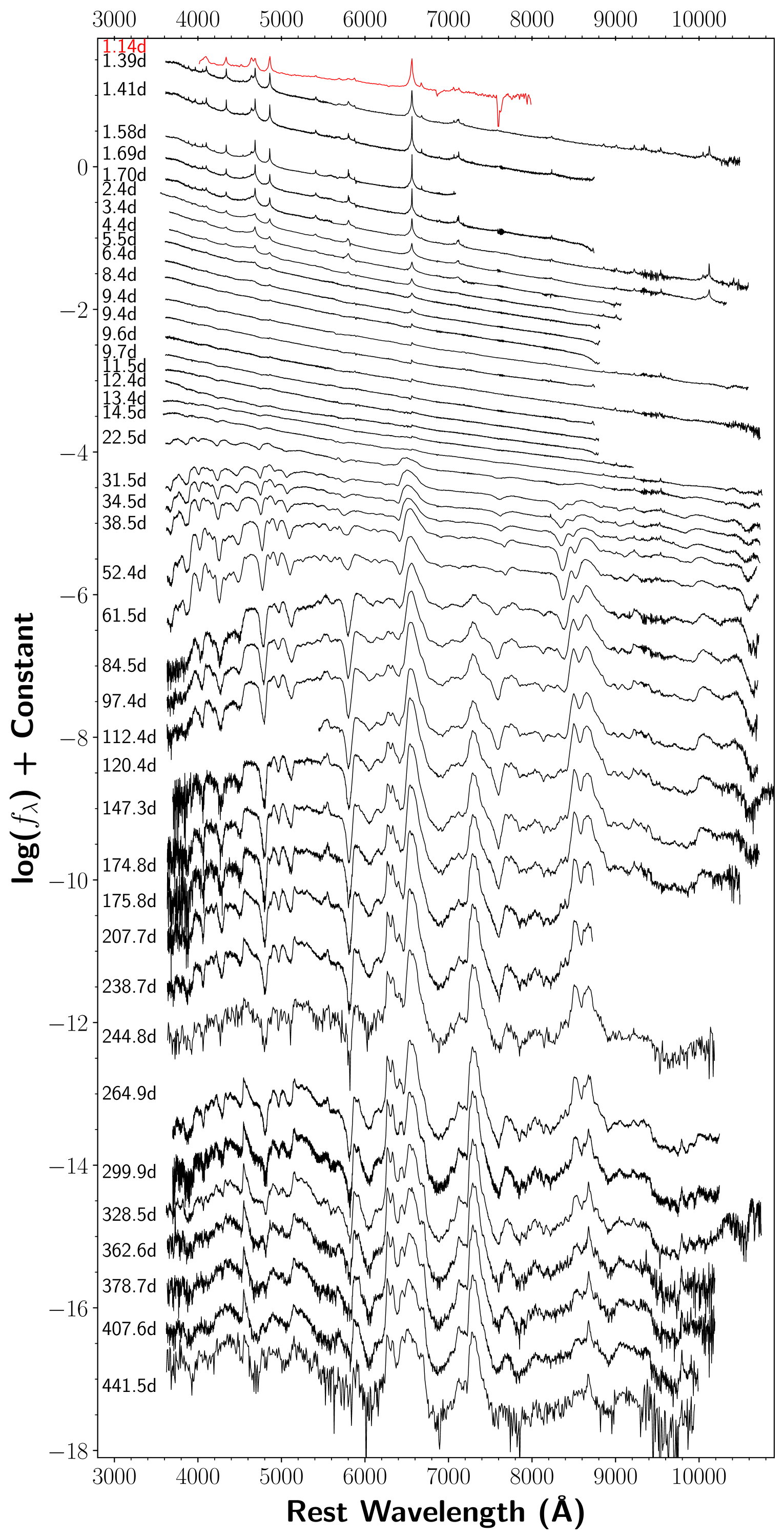
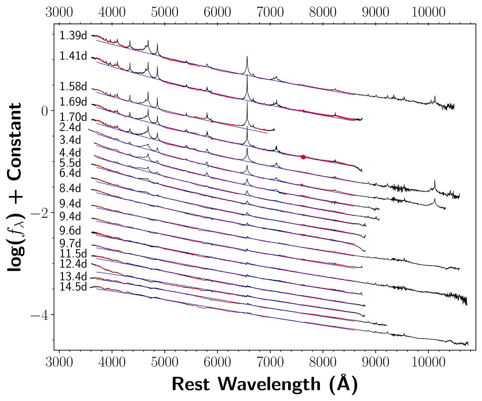
Figure 4 shows our full set of Kast spectra (a total of 42; see Table 1 for a full log) of SN 2023ixf until 442 days after explosion. Our first spectrum was taken at MJD = 60084.183, merely 1.39 days after explosion. We obtained nearly daily Kast spectra of SN 2023ixf for the first two weeks after explosion. In addition, for the first-night observations, we obtained 5 spectra ranging from 1.4 days to 1.7 days with different grating resolution with the same telescope (note that Bostroem et al. 2023 also obtained multiple spectra in the same night, but with different telescopes). These 5 spectra from the first-night observations were already shown by Zimmerman et al. (2024); also, the 3.4ḋ, 4.4 d, 5.5 d, 6.4 d, and 8.4 d spectra were presented by Jacobson-Galán et al. (2023), but we include them here for a more complete and detailed analysis. Augmenting the spectral set, we plot the the classification spectrum of SN 2023ixf at 1.14 days from the Liverpool telescope; this is the earliest reported spectrum of SN 2023ixf (Perley et al., 2023). These high-quality spectra allow us to perform thorough analysis of the spectral evolution of SN 2023ixf.
Distinct spectral evolution was seen from day 1.4 to day 442 as shown in Figure 4. We can classify the evolution into four main phases, following the suggestion given by Dessart et al. (2016) for SN 1998S. During the first few days, the most distinct features are the strong but narrow emission lines from the ionized CSM; we call this the CSM-dominated phase. These emission features weakened after the first week, so the spectra appear to be blue and quasi-featureless in the second week; this is the cold-dense-shell (CDS)-dominated phase, during which the only distinct features are from hydrogen, though weak and broad P Cygni features started to emerge at the end of the second week. After weeks, during the ejecta-dominated phase, the spectra are similar to those of other SNe II with strong P Cygni lines. After d, the spectra enter the nebular phase and forbidden lines start to form at late times. Detailed descriptions of each phase are given in the following sections.
4.1 CSM-Dominated Phase
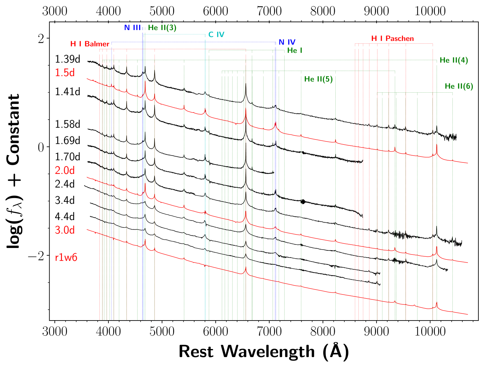
Figure 5 presents spectra of SN 2023ixf in the first 5 days during the CSM-dominated phase. During this phase, there are many both strong and weak narrow emission lines apparently caused by the ionized CSM, also reported by other groups (Jacobson-Galán et al., 2023; Bostroem et al., 2023; Hosseinzadeh et al., 2023; Hiramatsu et al., 2023; Teja et al., 2023; Yamanaka et al., 2023). These lines are also accompanied by broad components which are caused by electron scattering. We identified many species and found that most are from H and He.
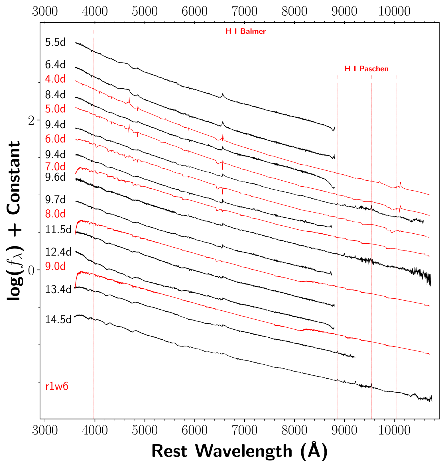
The strongest emission in the CSM-dominated phase is the H I Balmer series including H, H, H, H, H, H, and H, owing to the large abundance of hydrogen. As expected, H is the strongest line, with other Balmer lines gradually weaker at higher energy states (bluer wavelengths). In addition, the H I Paschen series also appears in our spectra at 1.41 d, 1.70 d, and 2.4 d. Although P 12,157 is outside our wavelength coverage, P, P, P, P, P, and P are clearly detected. However, the H I Paschen series is much weaker compared with the H I Balmer series. The H I Balmer and Paschen series are marked with red vertical lines in Figure 5.
| (Å) | (Å) | (Å) | (Å) | ||||
|---|---|---|---|---|---|---|---|
| 4 | 4685.70 | ||||||
| 5a | 3203.09 | 5 | 10123.59 | ||||
| 6 | 6560.09 | 6a | 18636.75 | ||||
| 7 | 5411.52 | 7a | 11626.41 | 7a | 30908.46 | ||
| 8 | 4859.32 | 8 | 9344.93 | 8a | 18743.33 | ||
| 9 | 4541.59 | 9 | 8236.79 | 9a | 14760.38 | ||
| 10 | 4338.68 | 10a | 7592.76 | 10a | 12812.83 | ||
| 11 | 4199.84 | 11 | 7177.53 | 11a | 11673.25 | ||
| 12 | 4100.05 | 12 | 6890.91 | 12a | 10933.62 | ||
| 13 | 4025.61 | 13 | 6683.21 | 13 | 10419.83 | ||
| 14a | 3968.44 | 14 | 6527.11 | 14 | 10045.27 | ||
| 15a | 3923.49 | 15 | 6406.39 | 15 | 9762.17 | ||
| 16 | 6310.86 | 16 | 9542.07 | ||||
| 17a | 6233.83 | 17 | 9367.05 | ||||
| 18 | 9225.25 | ||||||
| 19 | 9108.55 | ||||||
| 20a | 9011.23 | ||||||
| 21a | 8929.13 | ||||||
| 22a | 8859.17 | ||||||
| 23a | 8799.02 |
Helium also exhibits some strong emission lines. In fact, He II 4686 (at an energy state of ) is the second-strongest feature during the CSM-dominated phase. Moreover, a few other He II lines are detected from energy states , 5, and 6, marked as green vertical lines in Figure 5. A list of He II wavelengths from different energy states is given in Table 2, taken from the Atomic Data as part of CMFGEN444http://kookaburra.phyast.pitt.edu/hillier/web/CMFGEN.htm (Hillier & Dessart, 2012). Such complete He II series in SN spectra are presented here for the first time (to our knowledge), although some lines at higher energy states are too weak to be clearly detected. Higher signal-to-noise ratio (S/N) spectra could potentially reveal these weak lines in future SNe showing ionization features. In addition to He II, there are also a few He I lines detected; though much weaker, they are still quite obvious in our first-night spectra, including He I 5876, 6678, and 7065.
Besides hydrogen and helium, a few C and N features (marked as cyan and blue vertical lines) were also identified in the early-time spectra. C IV 5801, 5812 is not only detected, but even distinguished separately in our higher-resolution spectra on days 1.41, 1.58, and 1.69 (see also Smith et al. 2023 and Dickinson et al. 2024 with high-resolution spectroscopy). The detection of C IV 4658 is uncertain as it is blended with other lines. No lower ionization state C III lines are obviously detected; C III 4647, 4650 might be present, but it is blended with C IV 4658. N IV lines are also clearly detected with N IV 4058 and 7109, 7123. Lower ionization state N III 4634, 4641 is visible, but N III 4687 is blended with He II 4686 and thus uncertain. Both N IV 7109, 7123 and N III 4634, 4641 are also identified in our higher-resolution spectra on days 1.41, 1.58, and 1.69, similar to C IV 5801, 5812 (Smith et al. 2023 also show high-resolution spectra).
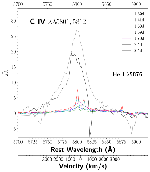
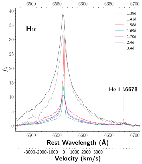
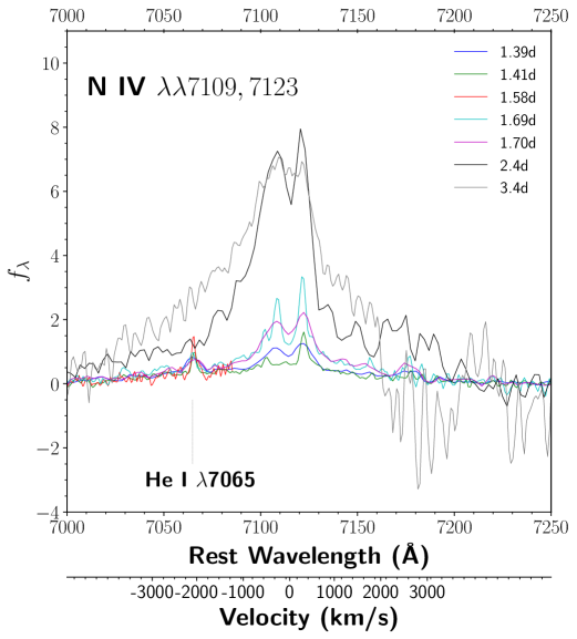
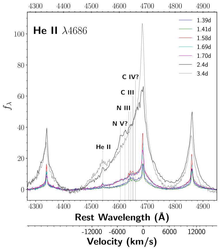
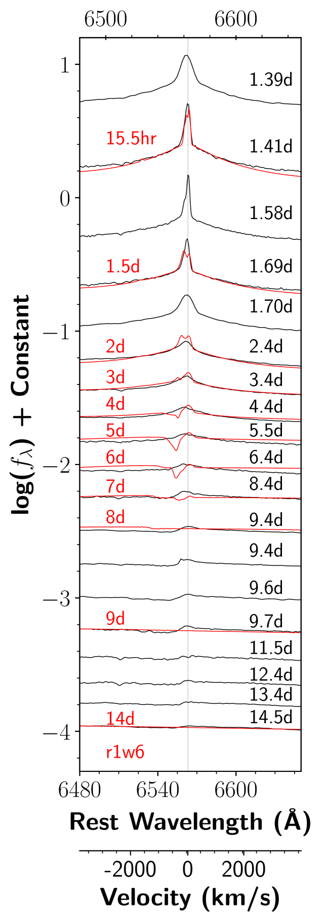
Interestingly, thanks to the total of 5 spectra taken during the first night of observations, we find that a few of the above-mentioned lines evolve quickly, showing intraday changes (see also Bostroem et al. 2023). For example, all three detected He I lines (5876, 6678, and 7065) weakened and almost disappeared from days 1.41 to 1.70, within 8 hr. To better illustrate this, in Figure 6 we plot the three He I regions centered on C IV 5801, 5812, H, and N IV 7115. By day 2.4 after explosion, all three He I lines disappeared completely. In addition, the N III 4634, 4641 and C III 4647, 4650 lines (blended) weakened quickly in the first two days, as shown in Figure 7 centered on He II 4686. The profile is very complicated, with many lines blended in the blue wing of He II 4686, including clear detections of C III 4647, 4650, N III 4634, 4641, and He II 4542, and possibly C IV 4658 and N V 4604, 4620. These lines boost the flux of the blue wing (while the red wing has a normal shape), making the He II profile very asymmetric. The emission blueward of He II 4686 even strengthens over the first few days, as shown in the right panel of Figure 7. Our highest-resolution spectrum at 1.58 d is able to distinguish both components of the N III 4634, 4641 doublet, which was even stronger in the 1.14 d spectrum from the Liverpool telescope, comparable to He II 4686, but weakened significantly to nearly undetected by day 1.70. Interestingly, there appears to be N V 4604, 4620 in the 2.4 d spectrum, but not earlier nor later. If real, this is additional evidence for intraday changes of the quickly evolving lines.
4.2 CDS-Dominated Phase
Overall, almost all the emission features faded away after about a week (except for the H I Balmer series, mainly H), and the spectra became quasi-featureless with a blue continuum during the second week, indicating that the ejecta are CDS dominated at this time, as shown in Figure 8. Because of this, one can try to fit the quasi-featureless spectra with a blackbody function to estimate the temperature of the ejecta, given the reliable relative flux calibration. To do so, we first correct the spectral extinction by adopting a total mag as mentioned above. We then exclude regions with obvious emission lines (we applied the same blackbody fitting to the spectra from the CSM-dominated phase, too). Finally, in order to keep consistent for spectra with different wavelength coverage at the red end, we restrict the fitting region to be below 8600 Å (the blue-end coverage is almost the same in all spectra). A blackbody function was applied to fit the spectra and the results are shown in Figure 9; the top panel indicates how well the blackbody function (blue) matches the selected data (red) by excluding the emission lines and the region beyond 8600 Å (black), and the bottom panel shows the evolution of the fitted temperature (blue circle) with time.
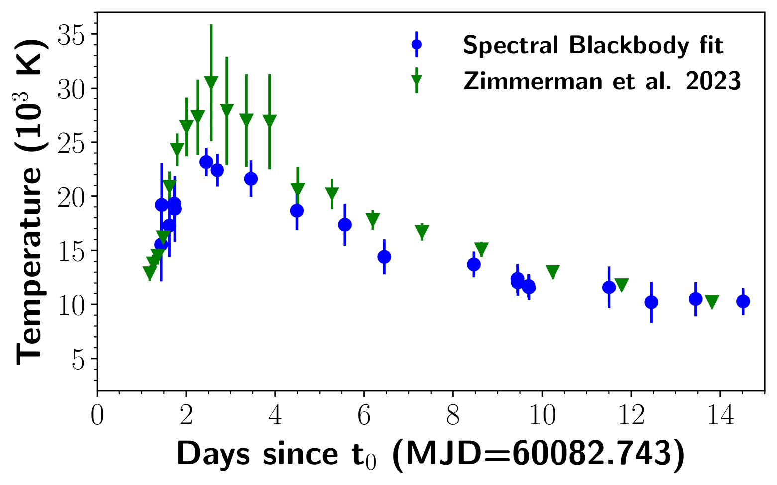
Our results demonstrate that the blackbody temperature rises quickly during the first few days, with K at 1.4 d and quickly reaching peak around 24,000 K about 2.5 days after explosion. The temperature then gradually drops in the next two weeks, and by day 14 it is K. For comparison, we also plot the temperature fitting results from Zimmerman et al. (2024) (green triangles), where they use the photometric fitting method (including UV photometry). Our results are generally consistent with theirs, though it appears that our fitted temperatures are slightly lower; however, our results are higher than the fitted temperatures given by Zhang et al. (2023a) (see their Fig. S3, middle panel).
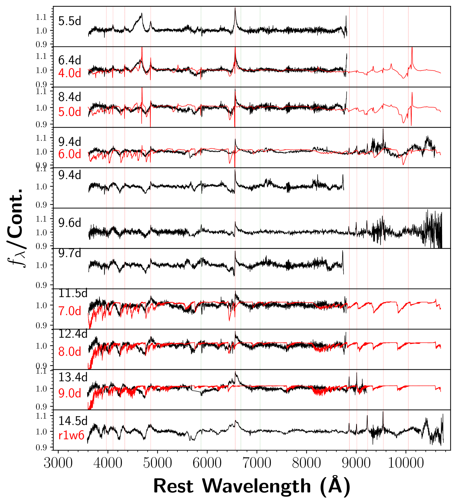
In order to better reveal the morphology of the weak lines in the quasi-featureless spectra, we adopt a normalization procedure following that of Leonard et al. (2000) (see their Fig. 5): the spectra are divided by the continuum, which was fitted with several-order splines by excluding obvious emission and absorption regions. The normalized spectra are shown in Figure 10.
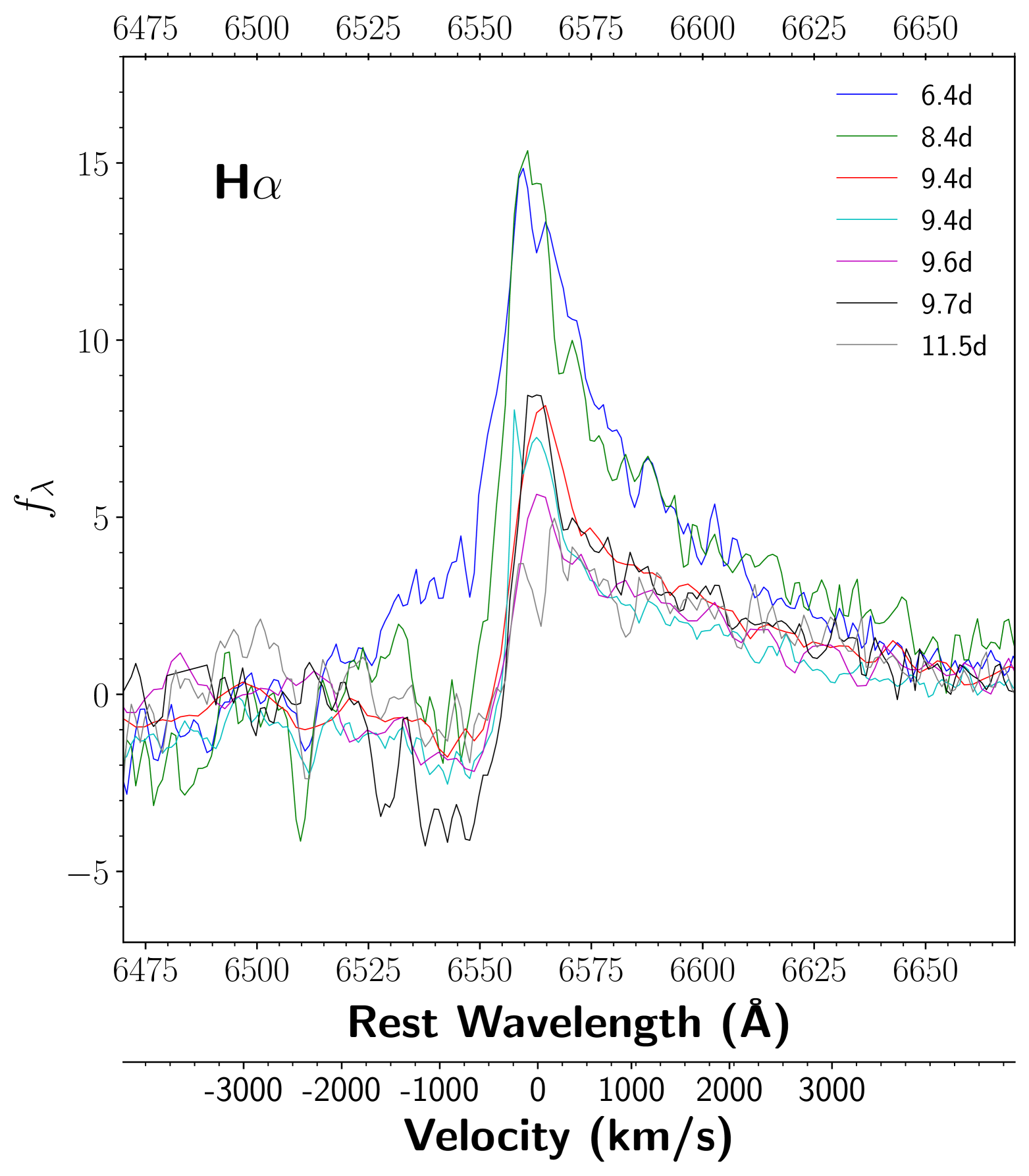
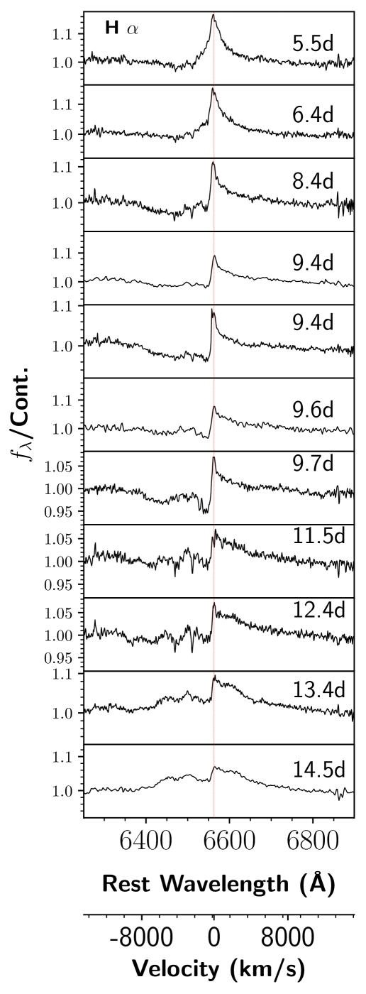
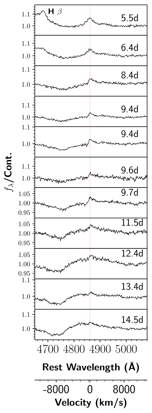
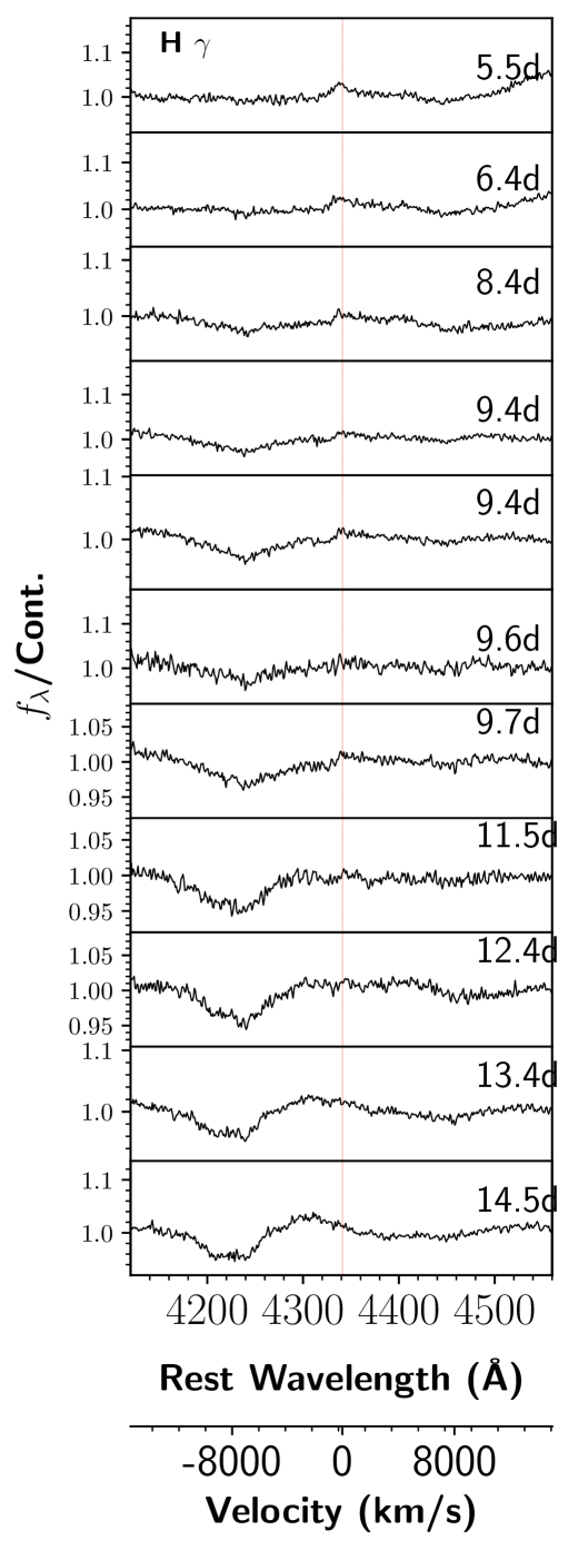
During this phase, one interesting feature is that the H line starts to show a low-velocity P Cygni profile on day 8.4, as shown in Figure 10 (also see Figs. 11 and 12). The velocity from the blue absorption minimum is km s-1 and lasts for about a week until day 14.5 (before a gap of our spectral coverage in the third week). Likely caused by radiative acceleration (Dessart, 2024), it is still unclear whether this mechanism could last for such a long time (see Sec. 4.5). However, there are no such low-velocity P Cygni features in the other H I Balmer lines beyond H (perhaps a weak signature in H on day 9; see the middle panel in Fig. 12). Instead, a broad P Cygni profile ( km s-1) starts to emerge in H, H, and H on day 8.4 (see next section for velocity measurements).
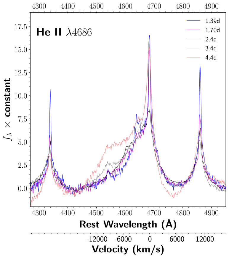
The H line at this phase does not exhibit a broad P Cygni profile, probably because the CDS at this phase is still optically thick. The H I Paschen series, however, remains as narrow emission until day 14.5. Unlike the H I Balmer lines, no low-velocity P Cygni nor broad P Cygni profiles are clearly seen in The H I Paschen series.
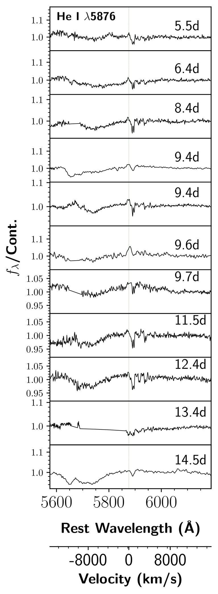
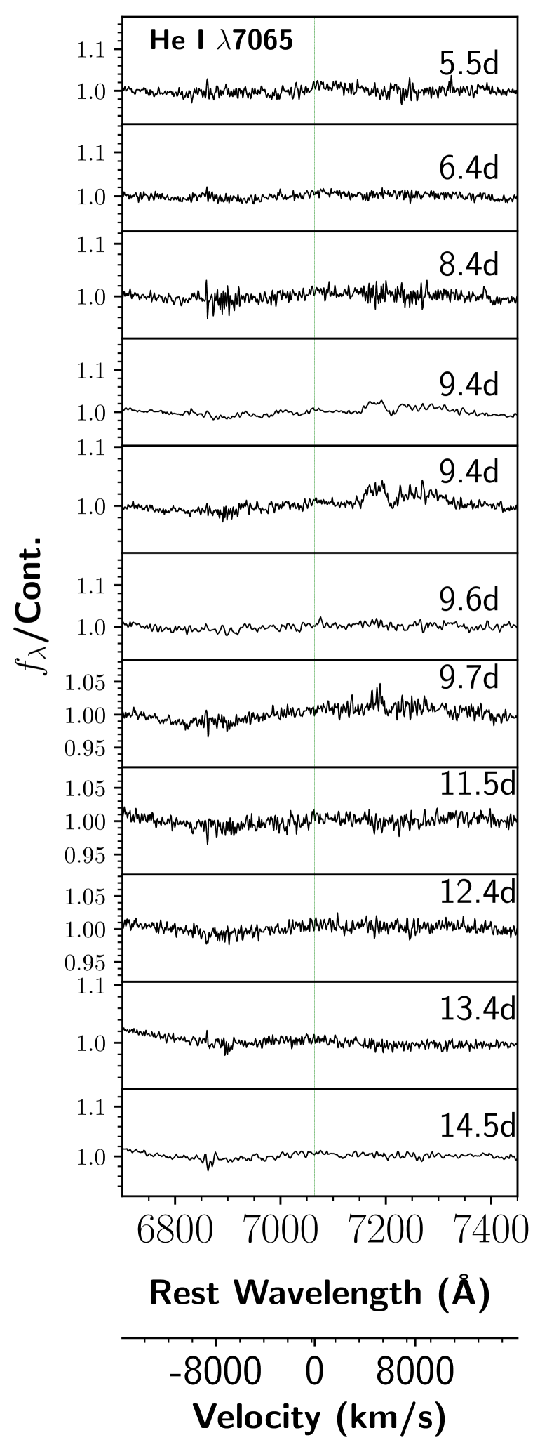
Interestingly, the He I lines which earlier disappeared (narrow emission lines) also start to be visible again, with broad P Cygni profiles around day 8, as shown in Figure 13. The He I 5876 profile in the left panel shows obvious absorption at a velocity of km s-1, though the absorption in the He I 7065 profile (right panel) is not significant. Also, there appears to be another bluer absorption in He I 5876 at 14.5 d with a velocity around 12,000 km s-1, which seems a bit high but not impossible.
4.3 Ejecta-Dominated Phase
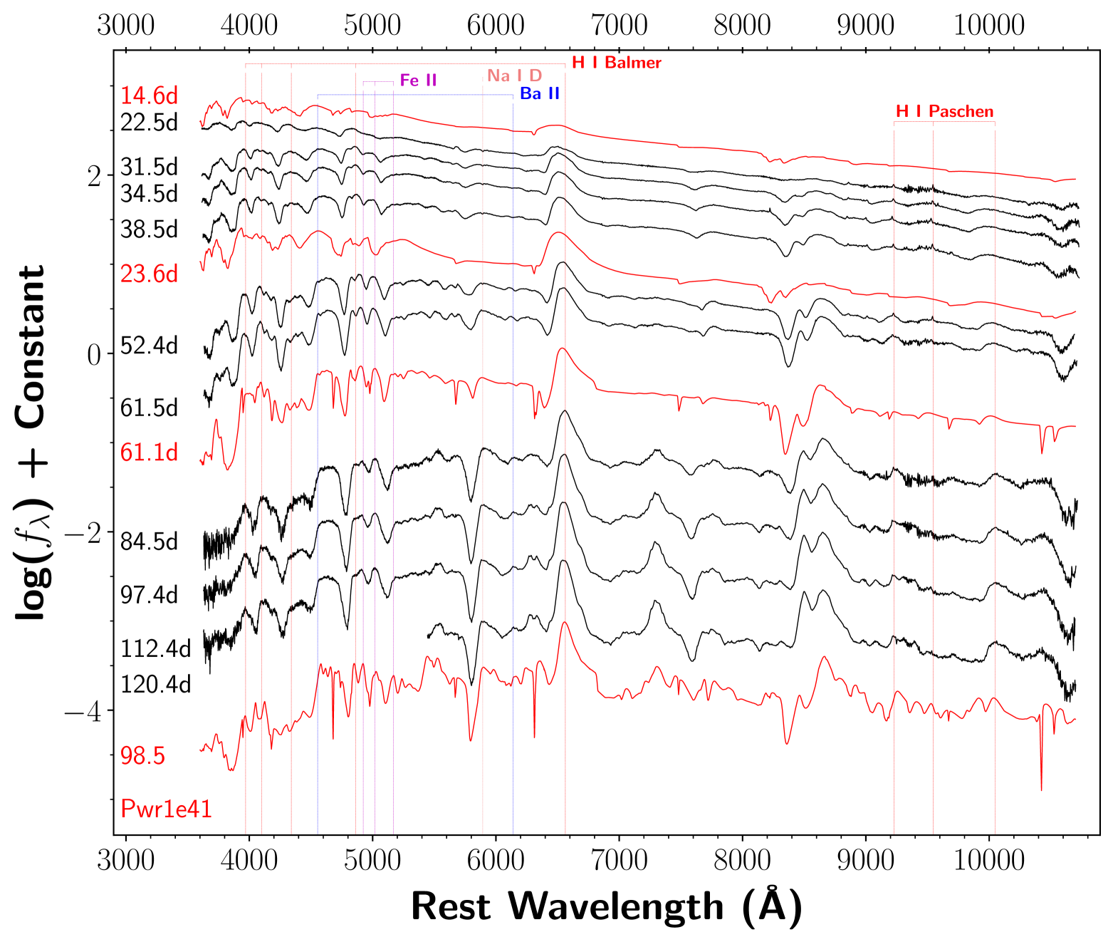
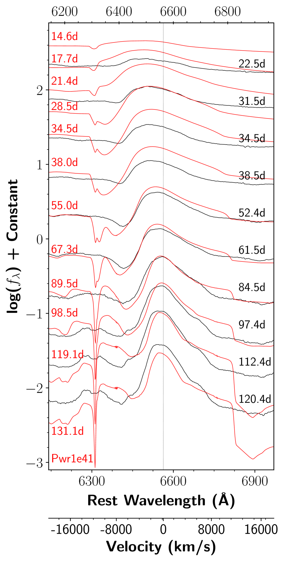
Owing to a lack of spectral coverage during the third week after explosion, the spectrum taken after 3 weeks (day 22.5 and thereafter) shows that the SN is ejecta dominated; there are many broad P Cygni features that are seen in normal SNe II. Figure 14 shows the spectra from days 22.5 to 120.4. Broad P Cygni profile of H I Balmer lines are very obvious, as well as a few other lines such as Fe II 4924, 5018, 5169.
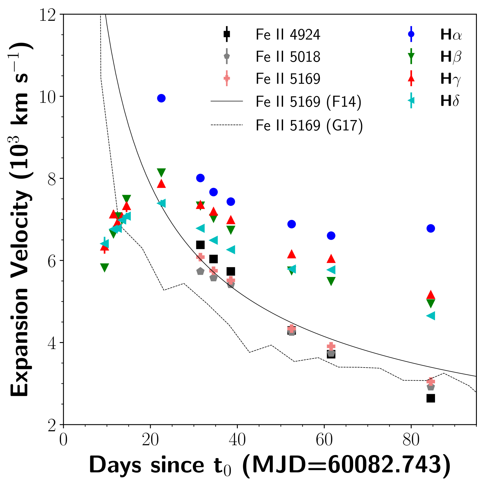
We measure the velocity from the blue absorption minimum of the broad P Cygni profile, and the results are shown in Figure 15. The velocity evolution after 3 weeks is typical of all lines compared with other normal SNe II; they all decline gradually with a power-law shape, with the H velocity higher than that of other lines. There is a dip blueward of H absorption from days 22.5 to 38.5, likely due to Si II 6355 at km s-1 (unlikely to be high-velocity H, which would be at km s-1). Si II 6355 is also predicted by the model (see model spectrum at 23.6 d in Fig. 14). However, the velocity of Si II 6355 ( km s-1) appears to be a bit low compared with H, so it is possible this is caused by some other line. The Fe II 4924, 5018, 5169 lines also evolve in a manner similar to that of Faran et al. (2014) as shown in Figure 15, though slightly higher than the results of Gutiérrez et al. (2017).
However, it is interesting to see that the velocities of H, H, and H (emerging earlier than H) at early times actually rise in the second week and reach their peak at days, km s-1. Such a velocity rise at early times is very unusual in SNe II, though it is predicted by some models (see, e.g., Fig. 9 of Dessart & Hillier 2010). This is likely not related to the unshocked CSM because the velocities are too high. Instead, it is a projection effect caused by sphericity (Dessart & Hillier, 2005, 2010).
4.4 Nebular Phase
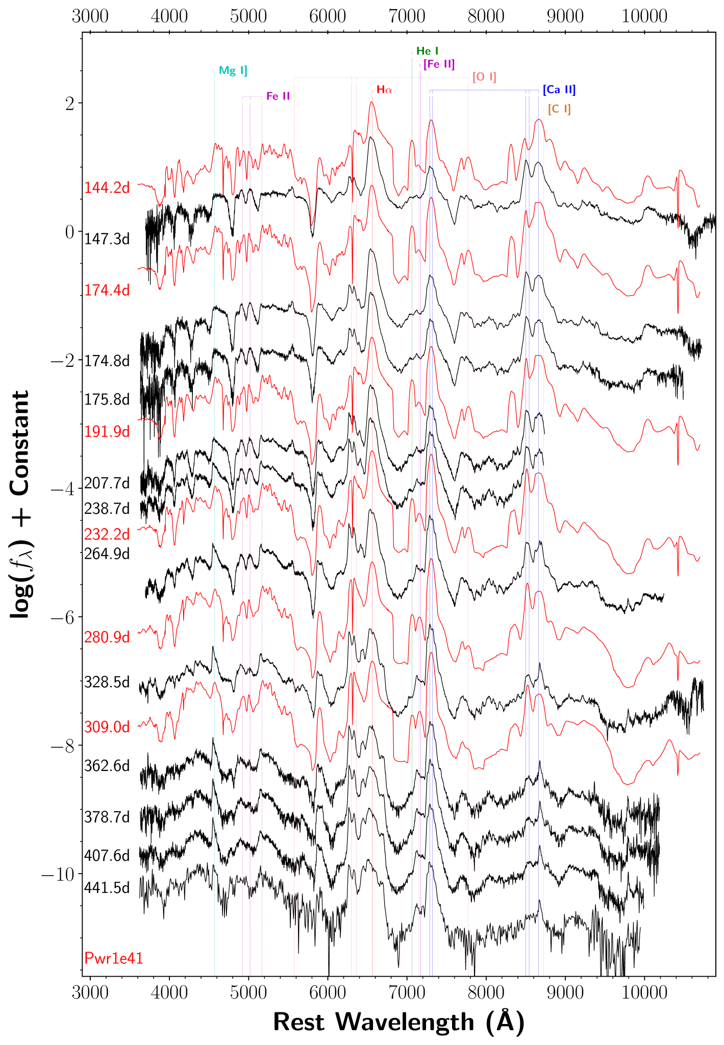
After d, the spectra enter the nebular phase and forbidden lines start to form at late times. Although H I Balmer lines remain the strongest features (mostly still absorption, as well as absorption from Fe II 4924, 5018, 5169), strong emission from forbidden lines also starts to emerge, such as [O I] 6300, 6364 and 7774, Mg I] 4571, [Ca II] 7291, 7323, and Ca II 8498, 8542, 8662, as shown in Figure 16.
4.5 Models and Physics
In order to produce the strongly ionized features (Gal-Yam et al., 2014) seen in the early-time spectra of SN 2023ixf, a certain amount of dense CSM is required surrounding the progenitor star, which could extend the shock-breakout time to days (compared to a timescale of hours if without dense CSM, thus difficult to detect). As the radiation leaks from the shock, UV photons are produced from the cooling of the shock-heated CSM, which then ionizes the CSM, forming these features. Such models were studied/simulated by Dessart et al. (2017, hereafter D17), where a set with different parameter spaces (radius, mass-loss rate, ejecta mass, etc.) were explored after explosion from an RSG progenitor. In fact, the progenitor of SN 2023ixf has been directly identified and confirmed to be an RSG (e.g., Kilpatrick et al., 2023; Soraisam et al., 2023; Van Dyk et al., 2024; Jencson et al., 2023; Pledger & Shara, 2023; Niu et al., 2023; Xiang et al., 2024; Qin et al., 2024), with an effective temperature, luminosity, and initial mass of K, , and 12–15 , respectively (Van Dyk et al., 2024). In the D17 models, r1w4 and r1w6 are the two showing strongly ionized features at early times, but r1w6 matches the evolution of SN 2023ixf better since the r1w4 model evolves too fast, so here we focus more on r1w6. For the r1w6 model, the following parameters were set: progenitor star radius (i.e., cm), mass-loss rate yr-1, extended CSM mass up to a distance of cm, and ejecta mass (see Table 1 and Sec. 3 in Dessart et al. 2017 for more details). A montage showing the evolution of the ejecta/CSM properties from the radiation hydrodynamical simulation of model r1w6 (Dessart et al., 2017) is plotted in Figure 17, where black, blue, and red lines respectively show the velocity, temperature, and luminosity along the radial distance at various epochs. The shaded area represents regions with .
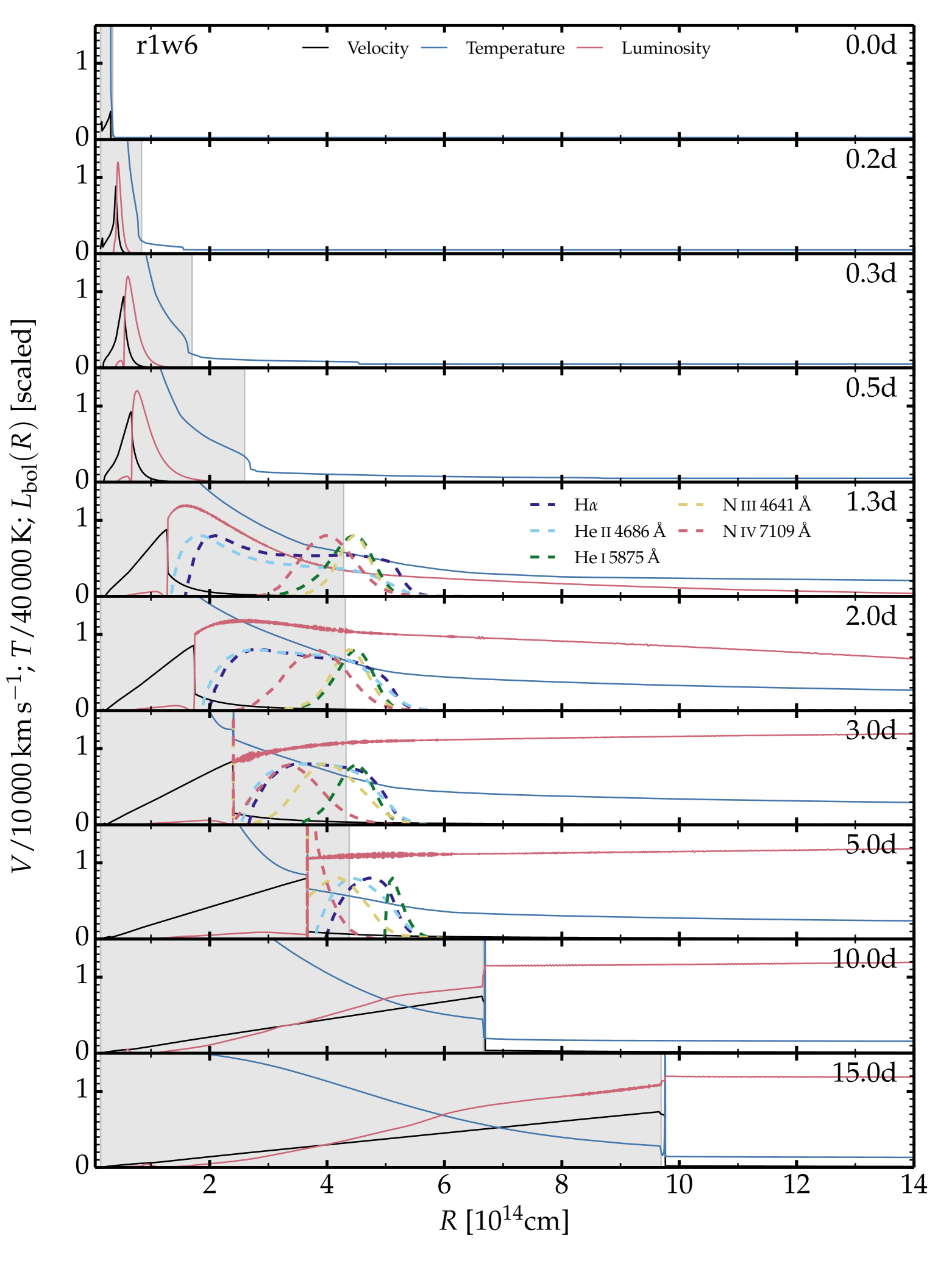
The r1w6 model spectra555Those used in this paper are slightly updated compared with the original r1w6 model given by D17 in which only H , He , CNO , and Fe were included. The updated models presented here include all important metals up to Nickel together with a more extended model atom for up to five ions per species (Fe I to Fe V) as well as number of levels etc. at 1.5 d, 2.0 d, and 3.0 d are plotted in Figure 5 in the CSM-dominated phase compared with the observed spectra. Overall, the model spectra match the observed spectra quite satisfactorily, including most of the major features such as the H I Balmer and Paschen series, all the He II series, C IV, N III, and N IV. However, there do exist some mismatches between the model spectra and the observed spectra. (1) As mentioned in Section 4.1, there are three He I lines (5876, 6678, and 7065) detected in the first-night spectra (days 1.41 to 1.70), yet they are not predicted (at least not obvious) in the model spectra666The He I lines are predicted in a slight variant of the r1w6 model presented by Jacobson-Galán et al. (2023); see their Figure 2., and they evolve quickly, showing intraday changes and almost disappearing within 8 hr. The disappearance of the He I lines is likely because of the quick increase of the temperature during the second day after explosion. As shown in Figure 9, the temperature rises quickly in the first 3 days, with K at 1.4 d and quickly reaches peak around 24,000 K at days after explosion. The He I lines require lower ionization energy (temperature); thus, at days, with lower temperatures, some He I lines formed and are detected in our spectra. As the temperature increase quickly and reaches its peak at d, most of the helium was ionized to He II, which requires a higher ionization energy (temperature) than He I, so He I almost disappears after two days, as predicted by the models too. (2) There appears to be N V 4604, 4620 in the 2.4 d spectrum, but not before nor after. If real, this is likely also because of the temperature changes. Typically, owing to temperature/ionization stratification in the CSM, the N V forms in the deepest layers of the CSM (i.e., closer to the shock where temperature is higher) as N V requires a very high ionization energy/temperature (there could also be a greater diversity in ionization if the CSM is asymmetric). At day 2.4, the temperature reached its peak, meeting the requirements to form N V lines (but not before the peak), and the temperature also decreases after the peak, so the N V disappeared thereafter. (3) The blue wing of He II 4686 is stronger and more asymmetric compared with the red wing, differing from the model spectra and were seen in some SNe (Jacobson-Galán et al., 2024b). Although the blue wing of He II 4686 is very complicated with many lines blended together (see Fig. 7), the flux in this region still seems to be too strong compared with the model spectra. This flux is therefore likely from the blueshifted emission of the fast-moving dense shell or the ejecta. The emission blueward of He II 4686 even strengthens in the first few days (see the right panel of Fig. 7), supporting the fact that we are seeing progressively more He II 4686 emission from the dense shell, which appears blueshifted at infinity due to optical-depth effects. The blueshifted emission eventually disappears after a week because He II recombines as the temperature drops.
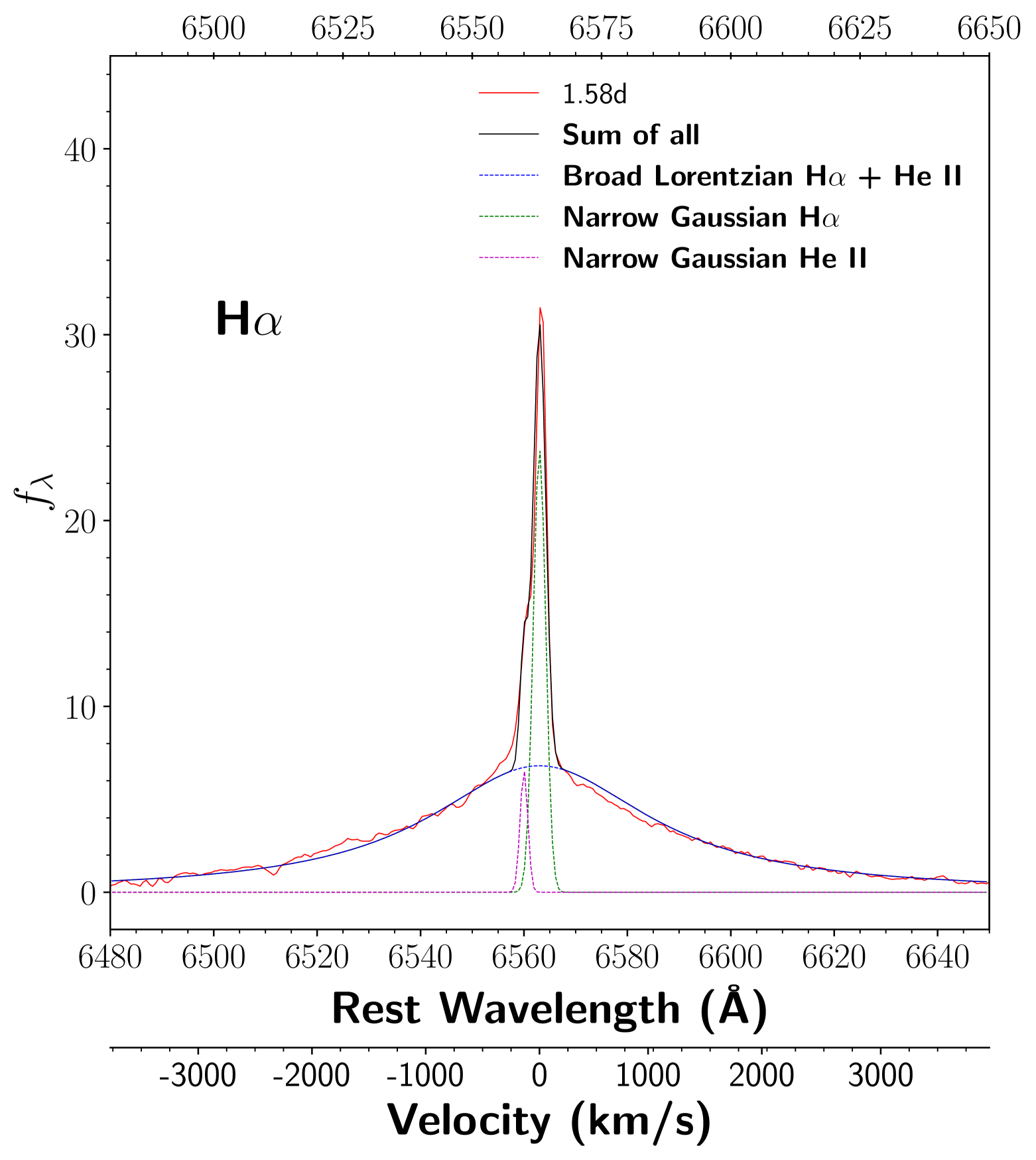
During the CSM-dominated phase, in the higher-resolution spectrum at 1.58 d we are able to distinguish He II 6560 from the blue wing of H, as shown in Figure 18. The ionized H luminosity can be used to estimate the mass-loss rate before explosion (Ofek et al., 2013). To do so, we follow the steps presented by Zhang et al. (2023a). We fit the H profile with three components: a narrow Gaussian component for He II 6560 (dashed cyan line), a narrow Gaussian component for H (dashed green line), and a wide Lorentzian component for both H and He II 6560 (dashed blue line) as shown in Figure 18. We only adopt one wide component for both H and He II 6560 because it is impossible to distinguish the two wide components given the small difference in central wavelength but very wide wings. We estimate the intrinsic FWHM of H to be km s-1, after removing by quadrature the instrumental FWHM of km s-1 (estimated from the night-sky emission lines) from the original measurement of km s-1. But note that the intrinsic FWHM of H measured at this time may have already been changed because of radiative acceleration, so it is more appropriate to consider this estimate as an upper limit of the intrinsic FWHM. The flux ratio between narrow H and He II 6560 is . The wide Lorentzian component gives a FWHM of km s-1, much broader than the narrow component. According to the relation (Ofek et al., 2013), we estimate the narrow H luminosity to be erg s-1. At 1.58 d we estimate the inner CSM distance (before swept up by the ejecta) to be cm (see method in next paragraph), so the mass-loss rate is found to be yr-1. But note that the broad H component carries much more flux777Measured to be about 10 times more, but only 60% is contributed by the broad H component, and 40% is contributed by the broad He II 6560 component, assuming the flux ratio is the same as for the narrow component. compared to the narrow H component; therefore, if counting the entire H luminosity, the estimated mass-loss rate would also be 6 times higher, yr-1. This value is lower than the mass-loss rate adopted by the r1w6 model of , likely because the calculation ignored the optical-depth effects in H.
The H profile broadens quickly after the first 2 days, as shown in the middle panel of Figure 6. The FWHM measured at 2.4 d and 3.4 d was km s-1. Interestingly, the FWHM measured from the wide Lorentzian component remains the same at km s-1, but still much broader than the narrow component.
After the first week of the SN explosion, the H starts to show a P Cygni profile with a minimum absorption velocity of km s-1, as shown in Figure 11 (see also left panel of Fig. 19). The P Cygni profile persists for more than a week (during this period, both the observed and r1w6 model spectra are mostly featureless as shown in Fig. 8). The broadening of H from km s-1 to km s-1 is unlikely to be caused by any outbursts or enhanced winds immediately before the explosion, but rather by radiative acceleration888An alternative explanation could be that we are seeing broad, boxy emission from the interaction with lower-density CSM, and that emission partially fills the H absorption. If the CSM is asymmetric and clumpy, this broad emission could be bumpy. as suggested by Zimmerman et al. (2024). However, the strong radiative acceleration mechanism requires the wind to have relatively low density, which means there is likely a big drop in the density profile following the shock breakout from the dense CSM. Since the P Cygni feature of H was detected as late as 14.5 d (after which the CSM would be swept up by the ejecta), by assuming a ejecta velocity of 10,000 km s-1 (as inferred from the highest H velocity in Fig. 15), one can calculate a distance of cm; the low-density CSM surrounding the progenitor was presented at least up to this distance. Similarly, one can also try to estimate the distance of the dense CSM from the shock breakout time, which is roughly equal to the temperature peak time, because once the shock breaks out, the CSM starts to cool. From the temperature evolution curve shown in Figure 9, we estimate the peak time to be day 2.5, thus giving a distance of cm. This is about 6 times the progenitor radius from the model.
The drop in the CSM radial density profile indicates an enhanced episode of mass loss at a certain time prior to the final core collapse. Assuming a wind velocity of 80 km s-1 (see above and Fig. 18), the promptly ejected matter would require days to reach a distance of cm. Since the typical RSG wind velocity is much smaller ( km s-1) than 80 km s-1, the actual delay time between the precursor event and the SN explosion could thus be longer, up to a few years. This could be consistent with the eruptive mass-loss scenario given by Hiramatsu et al. (2023), who favor eruptions releasing 0.3-–1 of the envelope at yr before explosion, although other possibilities are also discussed by Hiramatsu et al. (2023). However, such a high-mass eruption before the explosion could be at odds with the appearance of SN IIn-like spectral signatures because the photons cannot escape (see Dessart & Jacobson-Galán 2023); thus, a gradually enhanced episode of mass loss is more plausible. We also remark that the enhanced mass loss before the explosion inferred from the early-time spectral evolution of SN 2023ixf is corroborated by the semi-analytic fits to its early chromatic luminosity evolution (Li et al., 2024). The latter demand the presence of a dense CSM shell confined within a distance of a few to cm from the progenitor star, which is most likely to be produced through elevated mass loss at a rate of to yr-1 a few years before the SN explosion.
At the same (CDS-dominated) phase, the He I lines (which disappeared earlier) also start showing broad P Cygni profiles around day 8, as shown in Figures 10 and 13. He I 5876 has a velocity of 7000 km s-1 (He I 7065 is not very significant), similar to the velocity of H, H, and H at the same phase. The emergence of broad He I is also predicted by the r1w6 model (Fig. 10, red spectra) as the ejecta cool down and proceed to the recombination phase, though the model predicts the line to be present earlier (emerging on day 5 and disappearing by day 9).
On day 22, the broad P Cygni profile is well-developed and dominates the spectra. By this time, since the r1w6 model has no corresponding spectra at similar phases, we plot the shock-powered model Pwr1e41 (Dessart & Hillier, 2022) instead, as shown in Figure 14. In the Pwr1e41 model, a dense shell at 11,000 km s-1 was placed (which is very close to the ejecta velocity of km s-1 measured from H) to mimic the interaction of CSM at the earliest times and then a constant power of 1041 erg s-1. Since the model was developed in 1D, both the dense shell and the shock power are distributed in a spherical shell at 11,000 km s-1. We adopt the Pwr1e41 model here because it matches best with the observed spectra, including most of the major P Cygni features.
We also note that starting from day 84.5, a box-shaped component underlying the H profile emerges as indicated by the notch on its right side. The boxy profile is an indication of the continued interaction between the ejecta and the CSM confined within a radially extended shell. However, the boxy shape edge in the observed spectra shows a velocity of only km s-1 (see more details in Fig. 19, right panel), much smaller than the km s-1 ejecta velocity measured from H, which suggests an asymmetric dense shell or shock power (asymmetric wind). The Pwr1e41 model also clearly predicts the boxy profile at a higher velocity of 11,000 km s-1 (model input parameter), on both the red and blue sides. On the blue side, the box-shaped signature in the model spectra is a strong absorption feature at 11,000 km s-1, which persists in the model spectra since day 15 (see Fig. 19, right panel). However, such a strong feature is not clearly seen in the observed spectra, at least not before day 97 (there is a weak absorption feature after day 97 at similar velocity, but unclear whether it is related to the boxy profile). Instead, there is a boxy shape at km s-1, similar to the red side. If these two boxy profiles on both the blue and red side are connected (since they are at similar velocity), it would suggest a possible axial symmetry, as in a bipolar explosion.999Note that it could also be possible that the CDS of SN 2023ixf is actually only at km s-1, but this conflicts with the velocity measured from H of km s-1. In any case, since their velocities are much smaller than the ejecta velocity, it is an indication of an asymmetric dense shell, which may be related to the polarization. In fact, polarization of SN 2023ixf has been detected and reported at early phases (Vasylyev et al., 2023), and it further indicates that the CSM is indeed asymmetric. The asymmetry may help explain the observed lower velocity, as we might be seeing only the projected velocity along our line of sight, which is much lower than the model CDS velocity at 11,000 km s-1.
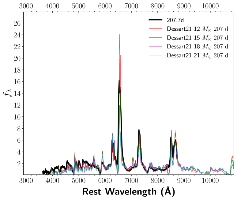
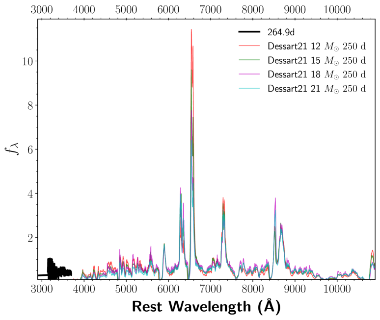
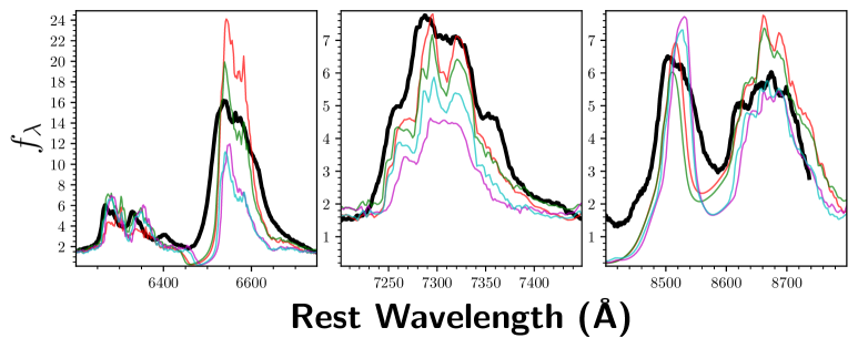
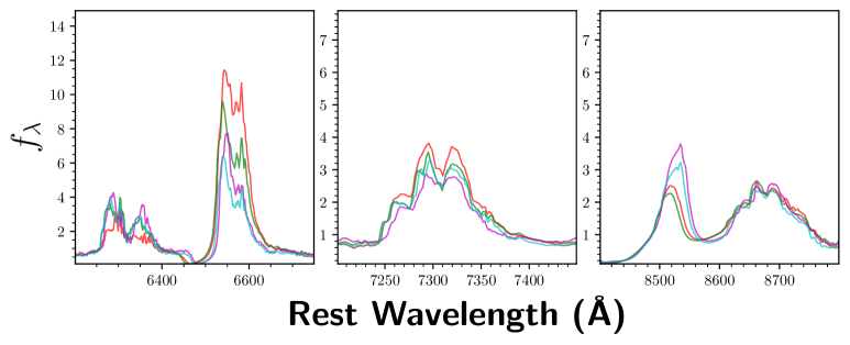
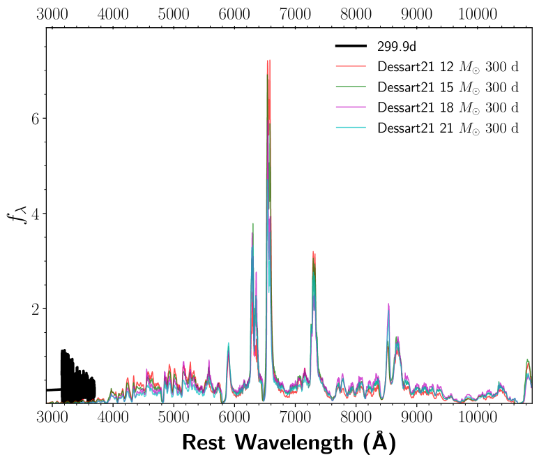
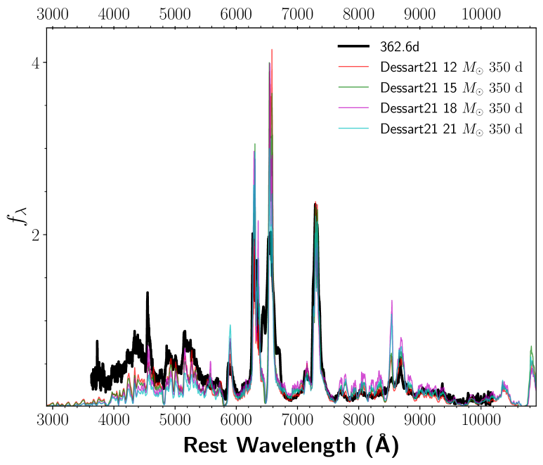
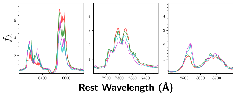
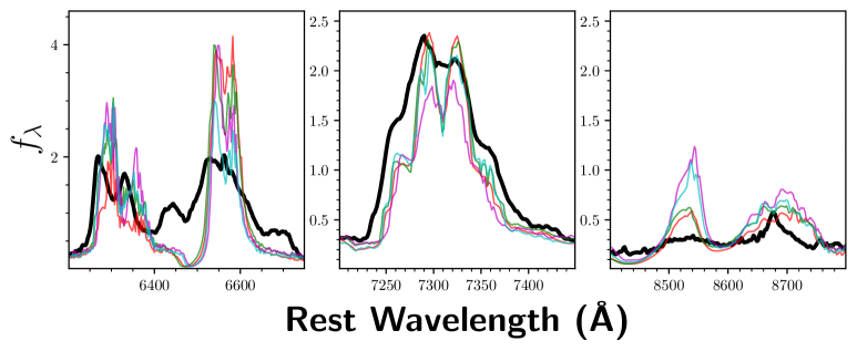
The nebular spectra can help us estimate the progenitor mass by comparing the observed spectra with the model spectra. We obtained several nebular spectra of SN 2023ixf at different phases. The model spectra were constructed based on the ejecta/progenitor models given by Dessart et al. (2021) and Sukhbold et al. (2016). Figure 20 shows the comparison at four epochs101010Note that Dessart et al. (2021) only showed model spectra at 350 d, other epochs model spectra were computed as part of this work.: 207.7 d, 264.9 d, 299.9 d, and 362.6 d. It appears that the model matches best with the observed nebular spectrum (followed by the model) for almost all the epochs. This is also consistent with the direct progenitor analysis by Van Dyk et al. (2024), who constrained the initial mass of the progenitor candidate from to . Comparing the four phases, we notice that the spectral flux decreased for all the lines except [Ca II] 7291, 7323 (middle of bottom zoomed-in panels for each phase in Fig. 20), which actually became stronger relative to Ca II 8498, 8542, 8662 (right side of bottom zoomed-in panels for each phase in Fig. 20). This is reasonable; as the ejecta grow more optically thin, the forbidden lines of Ca II strengthen relative to the permitted Ca II triplet. Also, note that the Fe II emission below 5500 Å is much stronger than in the model spectra; this might come from supersolar metallicity, or greater 56Ni mass, or (more likely) extra emission from interaction. Similarly, the nebular [Ca II] 7291, 7323 doublet on days 264.9 and 299.9 is also stronger than in the model spectra, which generally implies greater 56Ni since the line forms primarily from the 56Ni-rich material. Most lines also show broad emission, implying a sizable CDS contributing H and perhaps some Ca II. In addition, the “bridge” between H and [O I] 6300, 6364 is much stronger in the nebular spectra (left side of bottom zoomed-in panels for each phase in Fig. 20), a clear signature of a broad H emission from interaction. This means that some H emission is present at high blueshifted velocities, while it seems less present on the opposite, redshifted/receding part of the ejecta, linking to evidence of asymmetry at earlier times (i.e., asymmetry still prevails far from the star, although it is unclear whether this is the same geometry). In any case, the nebular spectrum until 362.6 d and even 441.5 d suggests that SN 2023ixf continues to interact (ever since shock breakout) with CSM produced by wind mass loss prior to the explosion.
5 Distance Measurement
M101 is a unique galaxy for testing our current methods to measure extragalatic distances. We have precise distance measurements from Cepheids (Freedman et al., 2001; Saha et al., 2006; Shappee & Stanek, 2011; Riess et al., 2022), TRGB(Rizzi et al., 2007; Shappee & Stanek, 2011; Beaton et al., 2019; Anand et al., 2022), and SNe Ia (Vinkó et al., 2012; Riess et al., 2022). The most recent measurements from those three techniques are all in good agreement. Using Cepheids, Riess et al. (2022) obtained a distance modulus of mag; with TRGB, Anand et al. (2022) obtained mag; and with SN 2011fe, Riess et al. (2022) measured mag.
However, the distance to M101 can also be derived using SN 2023ixf. Even if SNe II display a large range of peak luminosities, it has been demonstrated that they are excellent distance indicators. Using theoretical and empirical methods to calibrate them (de Jaeger & Galbany, 2023), we can measure distances with a precision of % (de Jaeger et al., 2020).
We focus our effort on the standard candle method (SCM; Hamuy et al., 2001), which is the most common and most accurate empirical technique used to derive SN II distances. Developed by Hamuy et al. (2001), it is based on the correlation between the SN absolute magnitude and two observables: the expansion velocity and the color. The expansion velocity is generally determined from the blueshift of Fe II or H P Cygni features. Using this technique, we obtain a distance of mag. This value is smaller than those derived from other techniques (Cepheids, TRGB, SNe Ia). The difference can be explained by the presence of strong CSM interaction (Hiramatsu et al., 2023), which boosts the luminosity above that of a normal SN II. The SCM is not able to correct for this effect, so the derived M101 distance from SN 2023ixf is likely too small. However, even if the distance is somewhat inaccurate, we can try to include SN 2023ixf as a calibrator to derive the Hubble-Lemaître constant through the distance-ladder technique. Adding SN 2023ixf to the 13 calibrators from de Jaeger et al. (2022), and using its Cepheid-based distance, we obtain H km s-1 Mpc-1 (statistical only) instead of H km s-1 Mpc-1 (de Jaeger et al., 2022). As expected, the uncertainties decrease because the number of calibrators increases (13 vs. 14), and the new value is smaller because SN 2023ixf is more luminous than the average SN II.
More recently, a theoretical method called the tailored expanding photosphere method has been developed by Vogl (2020). It is based on the expanding photosphere method (Kirshner & Kwan, 1974) but avoids the systematic distance uncertainties from the dilution factors. This method has been applied to several objects, yielding distance uncertainties smaller than 5% (Csörnyei et al., 2023). However, it cannot be used for SN 2023ixf because the radiative-transfer codes of Vogl (2020) do not include the strong CSM interaction seen in this object.
6 Conclusion and Discussion
We present both photometric and spectroscopic observations of SN 2023ixf covering from early times to the nebular phase. The light curves show that SN 2023ixf is in the fast decliner (IIL) subclass with a relatively short “plateau” phase (less than days), indicating an H-rich envelope of lower mass in the progenitor before explosion. It reached a peak -band absolute magnitude of mag, thus putting it at the bright end of SNe II.
Optical spectra show that SN 2023ixf transitioned from Type IIn to a typical Type II SN after three weeks. Early-time spectra of SN 2023ixf exhibit strong, narrow emission lines from the ionized CSM. We identified many species that produce these lines and found that most of them lines are from H and He, including He II series from energy states of , 5, and 6. The emission features weakened after the first week and the spectra appear to be blue and quasi-featureless in the second week, and can be fitted with a blackbody. After weeks, the spectra are similar to those of other SNe II, with strong P Cygni features, and the SN entered the nebular phase after about 6 months.
We compare observed spectra of SN 2023ixf with various model spectra in order to understand the physics behind SN 2023ixf. There is likely to be dense CSM surrounding the progenitor up to a distance of cm, followed by lower density CSM to distances of at least cm. Shortly before exploding, the progenitor may have had a mass-loss rate of up to yr-1. Our nebular spectra match best with a model spectrum.
SN 2023ixf is used as a distance indicator by fitting the light curves; we obtain a distance modulus of mag, slightly smaller than that derived from other techniques (Cepheids, TRGB, SN Ia), possibly because of strong CSM interaction in SN 2023ixf. By including SN 2023ixf as a calibrator and using its Cepheid distance, we obtain H km s-1 Mpc-1 (statistical only), slightly smaller (because SN 2023ixf is more luminous than the average SN II) but still in good agreement with H km s-1 Mpc-1 given by de Jaeger et al. (2022).
7 acknowledgments
A major upgrade of the Kast spectrograph on the Shane 3 m telescope at Lick Observatory, led by Brad Holden, was made possible through gifts from the Heising-Simons Foundation, William and Marina Kast, and the University of California Observatories. KAIT and its ongoing operation were made possible by donations from Sun Microsystems, Inc., the Hewlett-Packard Company, AutoScope Corporation, Lick Observatory, the U.S. National Science Foundation, the University of California, the Sylvia & Jim Katzman Foundation, and the TABASGO Foundation. Research at Lick Observatory is partially supported by a gift from Google. Some of the data presented herein were obtained at the W. M. Keck Observatory, which is operated as a scientific partnership among the California Institute of Technology, the University of California, and NASA; the observatory was made possible by the generous financial support of the W. M. Keck Foundation. We appreciate the expert assistance of the staffs at Lick and Keck Observatories.
We thank the following Lick Observatory Graduate Workshop participants for help obtaining Nickel photometry on two nights and Shane spectra on one night: Fangyi Cao, Casey Carlile, Madalyn Johnson, Zhexing Li, Ye Lin, Patrick Maloney, Michael McDonald, Pradyumna Sadhu, Loraine Sandoval Ascencio, Sogul Sanjaripour, Niloofar Sharei, Hurum Maksora Tohfa, and Michael Wozniak.
Generous financial support was provided to A.V.F.’s supernova group at U.C. Berkeley by the Christopher R. Redlich Fund, Steven Nelson, Sunil Nagaraj, Landon Noll, Sandy Otellini, Gary and Cynthia Bengier, Clark and Sharon Winslow, Alan Eustace, William Draper, Timothy and Melissa Draper, Briggs and Kathleen Wood, and Sanford Robertson (S.S.V. is a Steven Nelson Graduate Fellow in Astronomy, K.C.P. was a Nagaraj-Noll-Otellini Graduate Fellow in Astronomy, W.Z. is a Bengier-Winslow-Eustace Specialist in Astronomy, T.G.B. is a Draper-Wood-Robertson Specialist in Astronomy, Y.Y. was a Bengier-Winslow-Robertson Fellow in Astronomy). Numerous other donors to his group and/or research at Lick Observatory include Michael Antin, Duncan Beardsley, Jim Connelly and Anne Mackenzie, Curt and Shelley Covey, Byron and Allison Deeter, Arthur Folker, Tom and Dana Grogan, Heidi Gerster, Harvey Glasser, Charles and Gretchen Gooding, Tim and Judi Hachman, Alan and Gladys Hoefer, George Hume, Stephen Imbler, Michael Kast and Rebecca Lyon, Lata Krishnan and Ajay Shah, Walter Loewenstern, Rand Morimoto and Anna Henderson, Edward Oates, Doug Ogden, Jon and Susan Reiter, Cat Rondeau, Laura Sawczuk and Luke Ellis, Stan Schiffman, Richard Sesler, Justin and Seana Stephens, Ilya Strebulaev and Anna Dvornikova, Diane Tokugawa and Alan Gould, David and Joanne Turner, David and Malin Walrod, Gerry and Virginia Weiss, Janet Westin and Mike McCaw, David and Angie Yancey. A.S. acknowledges support from NASA/HST grant GO-17216. L.D. acknowledges access to the HPC resources of TGCC under the allocation 2023 – A0150410554 on Irene-Rome made by GENCI, France.
References
- Anand et al. (2022) Anand, G. S., Tully, R. B., Rizzi, L., Riess, A. G., & Yuan, W. 2022, ApJ, 932, 15, doi: 10.3847/1538-4357/ac68df
- Anderson et al. (2014) Anderson, J. P., González-Gaitán, S., Hamuy, M., et al. 2014, ApJ, 786, 67, doi: 10.1088/0004-637X/786/1/67
- Astropy Collaboration et al. (2013) Astropy Collaboration, Robitaille, T. P., Tollerud, E. J., et al. 2013, A&A, 558, A33, doi: 10.1051/0004-6361/201322068
- Astropy Collaboration et al. (2018) Astropy Collaboration, Price-Whelan, A. M., Sipőcz, B. M., et al. 2018, AJ, 156, 123, doi: 10.3847/1538-3881/aabc4f
- Beaton et al. (2019) Beaton, R. L., Seibert, M., Hatt, D., et al. 2019, ApJ, 885, 141, doi: 10.3847/1538-4357/ab4263
- Bonanos & Boumis (2016) Bonanos, A. Z., & Boumis, P. 2016, A&A, 585, A19, doi: 10.1051/0004-6361/201425412
- Bostroem et al. (2023) Bostroem, K. A., Pearson, J., Shrestha, M., et al. 2023, ApJ, 956, L5, doi: 10.3847/2041-8213/acf9a4
- Bruch et al. (2023) Bruch, R. J., Gal-Yam, A., Yaron, O., et al. 2023, ApJ, 952, 119, doi: 10.3847/1538-4357/acd8be
- Chufarin et al. (2023) Chufarin, V., Potapov, N., Ionov, I., et al. 2023, Transient Name Server AstroNote, 150, 1
- Csörnyei et al. (2023) Csörnyei, G., Vogl, C., Taubenberger, S., et al. 2023, A&A, 672, A129, doi: 10.1051/0004-6361/202245379
- de Jaeger & Galbany (2023) de Jaeger, T., & Galbany, L. 2023, arXiv e-prints, arXiv:2305.17243, doi: 10.48550/arXiv.2305.17243
- de Jaeger et al. (2022) de Jaeger, T., Galbany, L., Riess, A. G., et al. 2022, MNRAS, 514, 4620, doi: 10.1093/mnras/stac1661
- de Jaeger et al. (2019) de Jaeger, T., Zheng, W., Stahl, B. E., et al. 2019, MNRAS, 490, 2799, doi: 10.1093/mnras/stz2714
- de Jaeger et al. (2019) de Jaeger, T., Zheng, W., Stahl, B. E., et al. 2019, MNRAS, 490, 2799, doi: 10.1093/mnras/stz2714
- de Jaeger et al. (2020) de Jaeger, T., Galbany, L., González-Gaitán, S., et al. 2020, MNRAS, doi: 10.1093/mnras/staa1402
- Dessart (2024) Dessart, L. 2024, arXiv e-prints, arXiv:2405.04259, doi: 10.48550/arXiv.2405.04259
- Dessart & Hillier (2005) Dessart, L., & Hillier, D. J. 2005, A&A, 439, 671, doi: 10.1051/0004-6361:20053217
- Dessart & Hillier (2010) —. 2010, MNRAS, 405, 2141, doi: 10.1111/j.1365-2966.2010.16611.x
- Dessart & Hillier (2022) —. 2022, A&A, 660, L9, doi: 10.1051/0004-6361/202243372
- Dessart et al. (2017) Dessart, L., Hillier, D. J., & Audit, E. 2017, A&A, 605, A83, doi: 10.1051/0004-6361/201730942
- Dessart et al. (2016) Dessart, L., Hillier, D. J., Audit, E., Livne, E., & Waldman, R. 2016, MNRAS, 458, 2094, doi: 10.1093/mnras/stw336
- Dessart et al. (2021) Dessart, L., Hillier, D. J., Sukhbold, T., Woosley, S. E., & Janka, H. T. 2021, A&A, 652, A64, doi: 10.1051/0004-6361/202140839
- Dessart & Jacobson-Galán (2023) Dessart, L., & Jacobson-Galán, W. V. 2023, A&A, 677, A105, doi: 10.1051/0004-6361/202346754
- Dickinson et al. (2024) Dickinson, D., Milisavljevic, D., Garretson, B., et al. 2024, arXiv e-prints, arXiv:2412.14406, doi: 10.48550/arXiv.2412.14406
- Faran et al. (2014) Faran, T., Poznanski, D., Filippenko, A. V., et al. 2014, MNRAS, 442, 844, doi: 10.1093/mnras/stu955
- Filippenko (1982) Filippenko, A. V. 1982, PASP, 94, 715, doi: 10.1086/131052
- Filippenko (1989) —. 1989, AJ, 97, 726, doi: 10.1086/115018
- Filippenko (1991a) Filippenko, A. V. 1991a, in Supernovae, ed. S. E. Woosley, 467
- Filippenko (1991b) Filippenko, A. V. 1991b, in European Southern Observatory Conference and Workshop Proceedings, Vol. 37, European Southern Observatory Conference and Workshop Proceedings, ed. I. J. Danziger & K. Kjaer
- Filippenko (1997) Filippenko, A. V. 1997, Annual Review of A & A, 35, 309, doi: 10.1146/annurev.astro.35.1.309
- Filippenko et al. (2001) Filippenko, A. V., Li, W. D., Treffers, R. R., & Modjaz, M. 2001, in Astronomical Society of the Pacific Conference Series, Vol. 246, IAU Colloq. 183: Small Telescope Astronomy on Global Scales, ed. B. Paczynski, W.-P. Chen, & C. Lemme, 121
- Filippenko et al. (2023) Filippenko, A. V., Zheng, W., & Yang, Y. 2023, Transient Name Server AstroNote, 123, 1. https://ui.adsabs.harvard.edu/abs/2023TNSAN.123....1F
- Freedman et al. (2001) Freedman, W. L., Madore, B. F., Gibson, B. K., et al. 2001, ApJ, 553, 47, doi: 10.1086/320638
- Fulton et al. (2023) Fulton, M. D., Nicholl, M., Smith, K. W., et al. 2023, Transient Name Server AstroNote, 124, 1
- Gal-Yam et al. (2014) Gal-Yam, A., Arcavi, I., Ofek, E. O., et al. 2014, Nature, 509, 471, doi: 10.1038/nature13304
- Galbany et al. (2016) Galbany, L., Hamuy, M., Phillips, M. M., et al. 2016, AJ, 151, 33, doi: 10.3847/0004-6256/151/2/33
- Gutiérrez et al. (2017) Gutiérrez, C. P., Anderson, J. P., Hamuy, M., et al. 2017, ApJ, 850, 89, doi: 10.3847/1538-4357/aa8f52
- Hamann (2023) Hamann, N. 2023, Transient Name Server AstroNote, 127, 1
- Hamuy & Pinto (2002) Hamuy, M., & Pinto, P. A. 2002, ApJ, 566, L63, doi: 10.1086/339676
- Hamuy et al. (2001) Hamuy, M., Pinto, P. A., Maza, J., et al. 2001, ApJ, 558, 615, doi: 10.1086/322450
- Henden et al. (2012) Henden, A., Krajci, T., & Munari, U. 2012, Information Bulletin on Variable Stars, 6024, 1
- Hillier & Dessart (2012) Hillier, D. J., & Dessart, L. 2012, MNRAS, 424, 252, doi: 10.1111/j.1365-2966.2012.21192.x
- Hillier & Dessart (2019) —. 2019, A&A, 631, A8, doi: 10.1051/0004-6361/201935100
- Hiramatsu et al. (2021) Hiramatsu, D., Howell, D. A., Moriya, T. J., et al. 2021, ApJ, 913, 55, doi: 10.3847/1538-4357/abf6d6
- Hiramatsu et al. (2023) Hiramatsu, D., Tsuna, D., Berger, E., et al. 2023, ApJ, 955, L8, doi: 10.3847/2041-8213/acf299
- Hosseinzadeh et al. (2023) Hosseinzadeh, G., Farah, J., Shrestha, M., et al. 2023, ApJ, 953, L16, doi: 10.3847/2041-8213/ace4c4
- Itagaki (2023) Itagaki, K. 2023, Transient Name Server Discovery Report, 2023-1158, 1
- Jacobson-Galán et al. (2022) Jacobson-Galán, W. V., Dessart, L., Jones, D. O., et al. 2022, ApJ, 924, 15, doi: 10.3847/1538-4357/ac3f3a
- Jacobson-Galán et al. (2023) Jacobson-Galán, W. V., Dessart, L., Margutti, R., et al. 2023, ApJ, 954, L42, doi: 10.3847/2041-8213/acf2ec
- Jacobson-Galán et al. (2024a) Jacobson-Galán, W. V., Dessart, L., Davis, K. W., et al. 2024a, ApJ, 970, 189, doi: 10.3847/1538-4357/ad4a2a
- Jacobson-Galán et al. (2024b) —. 2024b, ApJ, 970, 189, doi: 10.3847/1538-4357/ad4a2a
- Jencson et al. (2023) Jencson, J. E., Pearson, J., Beasor, E. R., et al. 2023, ApJ, 952, L30, doi: 10.3847/2041-8213/ace618
- Kilpatrick et al. (2023) Kilpatrick, C. D., Foley, R. J., Jacobson-Galán, W. V., et al. 2023, ApJ, 952, L23, doi: 10.3847/2041-8213/ace4ca
- Kirshner & Kwan (1974) Kirshner, R. P., & Kwan, J. 1974, ApJ, 193, 27, doi: 10.1086/153123
- Koltenbah (2023) Koltenbah, B. 2023, Transient Name Server AstroNote, 144, 1
- Landolt (1992) Landolt, A. U. 1992, AJ, 104, 340, doi: 10.1086/116242
- Landsman (1993) Landsman, W. B. 1993, 52, 246. https://ui.adsabs.harvard.edu/abs/1993ASPC...52..246L
- Leonard et al. (2000) Leonard, D. C., Filippenko, A. V., Barth, A. J., & Matheson, T. 2000, ApJ, 536, 239, doi: 10.1086/308910
- Li et al. (2024) Li, G., Hu, M., Li, W., et al. 2024, Nature, 627, 754, doi: 10.1038/s41586-023-06843-6
- Li et al. (2003) Li, W., Filippenko, A. V., Chornock, R., & Jha, S. 2003, PASP, 115, 844, doi: 10.1086/376432
- Limeburner (2023) Limeburner, S. 2023, Transient Name Server AstroNote, 128, 1
- Mao et al. (2023) Mao, Y., Zhang, M., Cai, G., et al. 2023, TNS, 130, 1. https://ui.adsabs.harvard.edu/abs/2023TNSAN.130....1M
- Miller & Stone (1994) Miller, J., & Stone, R. 1994, The Kast Double Spectrograph
- Morozova et al. (2015) Morozova, V., Piro, A. L., Renzo, M., et al. 2015, ApJ, 814, 63, doi: 10.1088/0004-637X/814/1/63
- Niu et al. (2023) Niu, Z., Sun, N.-C., Maund, J. R., et al. 2023, ApJ, 955, L15, doi: 10.3847/2041-8213/acf4e3
- Ofek et al. (2013) Ofek, E. O., Lin, L., Kouveliotou, C., et al. 2013, ApJ, 768, 47, doi: 10.1088/0004-637X/768/1/47
- Perley et al. (2023) Perley, D. A., Gal-Yam, A., Irani, I., & Zimmerman, E. 2023, Transient Name Server AstroNote, 119, 1
- Perley & Irani (2023) Perley, D. A., & Irani, I. 2023, Transient Name Server AstroNote, 120, 1
- Pledger & Shara (2023) Pledger, J. L., & Shara, M. M. 2023, ApJ, 953, L14, doi: 10.3847/2041-8213/ace88b
- Qin et al. (2024) Qin, Y.-J., Zhang, K., Bloom, J., et al. 2024, MNRAS, 534, 271, doi: 10.1093/mnras/stae2012
- Ransome et al. (2021) Ransome, C. L., Habergham-Mawson, S. M., Darnley, M. J., et al. 2021, MNRAS, 506, 4715, doi: 10.1093/mnras/stab1938
- Riess et al. (2022) Riess, A. G., Yuan, W., Macri, L. M., et al. 2022, ApJ Letters, 934, L7, doi: 10.3847/2041-8213/ac5c5b
- Riess et al. (2022) Riess, A. G., Yuan, W., Macri, L. M., et al. 2022, ApJ, 934, L7, doi: 10.3847/2041-8213/ac5c5b
- Rizzi et al. (2007) Rizzi, L., Tully, R. B., Makarov, D., et al. 2007, ApJ, 661, 815, doi: 10.1086/516566
- Saha et al. (2006) Saha, A., Thim, F., Tammann, G. A., Reindl, B., & Sandage, A. 2006, ApJS, 165, 108, doi: 10.1086/503800
- Sanders et al. (2015) Sanders, N. E., Soderberg, A. M., Gezari, S., et al. 2015, ApJ, 799, 208, doi: 10.1088/0004-637X/799/2/208
- Schlafly & Finkbeiner (2011) Schlafly, E. F., & Finkbeiner, D. P. 2011, ApJ, 737, 103, doi: 10.1088/0004-637X/737/2/103
- Schlegel (1990) Schlegel, E. M. 1990, MNRAS, 244, 269
- Sgro et al. (2023) Sgro, L. A., Esposito, T. M., Blaclard, G., et al. 2023, Research Notes of the American Astronomical Society, 7, 141, doi: 10.3847/2515-5172/ace41f
- Shappee & Stanek (2011) Shappee, B. J., & Stanek, K. Z. 2011, ApJ, 733, 124, doi: 10.1088/0004-637X/733/2/124
- Silverman et al. (2012) Silverman, J. M., Foley, R. J., Filippenko, A. V., et al. 2012, MNRAS, 425, 1789, doi: 10.1111/j.1365-2966.2012.21270.x
- Smartt (2009) Smartt, S. J. 2009, ARA&A, 47, 63, doi: 10.1146/annurev-astro-082708-101737
- Smartt (2015) —. 2015, PASA, 32, e016, doi: 10.1017/pasa.2015.17
- Smith et al. (2023) Smith, N., Pearson, J., Sand, D. J., et al. 2023, ApJ, 956, 46, doi: 10.3847/1538-4357/acf366
- Soraisam et al. (2023) Soraisam, M. D., Szalai, T., Van Dyk, S. D., et al. 2023, ApJ, 957, 64, doi: 10.3847/1538-4357/acef22
- Stahl et al. (2019) Stahl, B. E., Zheng, W., de Jaeger, T., et al. 2019, MNRAS, 490, 3882, doi: 10.1093/mnras/stz2742
- Stathakis & Sadler (1991) Stathakis, R. A., & Sadler, E. M. 1991, MNRAS, 250, 786, doi: 10.1093/mnras/250.4.786
- Stetson (1987) Stetson, P. B. 1987, PASP, 99, 191, doi: 10.1086/131977
- Sukhbold et al. (2016) Sukhbold, T., Ertl, T., Woosley, S. E., Brown, J. M., & Janka, H. T. 2016, ApJ, 821, 38, doi: 10.3847/0004-637X/821/1/38
- Tartaglia et al. (2021) Tartaglia, L., Sand, D. J., Groh, J. H., et al. 2021, ApJ, 907, 52, doi: 10.3847/1538-4357/abca8a
- Teja et al. (2023) Teja, R. S., Singh, A., Basu, J., et al. 2023, ApJ, 954, L12, doi: 10.3847/2041-8213/acef20
- Terreran et al. (2016) Terreran, G., Jerkstrand, A., Benetti, S., et al. 2016, MNRAS, 462, 137, doi: 10.1093/mnras/stw1591
- Terreran et al. (2022) Terreran, G., Jacobson-Galán, W. V., Groh, J. H., et al. 2022, ApJ, 926, 20, doi: 10.3847/1538-4357/ac3820
- Tody (1986) Tody, D. 1986, in Society of Photo-Optical Instrumentation Engineers (SPIE) Conference Series, Vol. 627, Instrumentation in astronomy VI, ed. D. L. Crawford, 733, doi: 10.1117/12.968154
- Valenti et al. (2016) Valenti, S., Howell, D. A., Stritzinger, M. D., et al. 2016, MNRAS, 459, 3939, doi: 10.1093/mnras/stw870
- Van Dyk (2017) Van Dyk, S. D. 2017, Philosophical Transactions of the Royal Society of London Series A, 375, 20160277, doi: 10.1098/rsta.2016.0277
- Van Dyk et al. (2003) Van Dyk, S. D., Li, W., & Filippenko, A. V. 2003, PASP, 115, 1289, doi: 10.1086/378308
- Van Dyk et al. (2000) Van Dyk, S. D., Peng, C. Y., King, J. Y., et al. 2000, PASP, 112, 1532, doi: 10.1086/317727
- Van Dyk et al. (2019) Van Dyk, S. D., Zheng, W., Maund, J. R., et al. 2019, ApJ, 875, 136, doi: 10.3847/1538-4357/ab1136
- Van Dyk et al. (2024) Van Dyk, S. D., Srinivasan, S., Andrews, J. E., et al. 2024, ApJ, 968, 27, doi: 10.3847/1538-4357/ad414b
- Vasylyev et al. (2023) Vasylyev, S. S., Yang, Y., Filippenko, A. V., et al. 2023, ApJ, 955, L37, doi: 10.3847/2041-8213/acf1a3
- Vinkó et al. (2012) Vinkó, J., Sárneczky, K., Takáts, K., et al. 2012, A&A, 546, A12, doi: 10.1051/0004-6361/201220043
- Vogl (2020) Vogl, C. 2020, PhD thesis, Technical University of Munich, Germany
- Xiang et al. (2024) Xiang, D., Mo, J., Wang, L., et al. 2024, Science China Physics, Mechanics, and Astronomy, 67, 219514, doi: 10.1007/s11433-023-2267-0
- Yamanaka et al. (2023) Yamanaka, M., Fujii, M., & Nagayama, T. 2023, PASJ, 75, L27, doi: 10.1093/pasj/psad051
- Yaron et al. (2023) Yaron, O., Bruch, R., Chen, P., et al. 2023, Transient Name Server AstroNote, 133, 1
- Yaron et al. (2017) Yaron, O., Perley, D. A., Gal-Yam, A., et al. 2017, Nature Physics, 13, 510, doi: 10.1038/nphys4025
- Zhang et al. (2023a) Zhang, J., Lin, H., Wang, X., et al. 2023a, Science Bulletin, 68, 2548, doi: 10.1016/j.scib.2023.09.015
- Zhang et al. (2023b) Zhang, K., Kennedy, D., Oostermeyer, B., Bloom, J., & Perley, D. A. 2023b, Transient Name Server AstroNote, 125, 1
- Zimmerman et al. (2024) Zimmerman, E. A., Irani, I., Chen, P., et al. 2024, Nature, 627, 759, doi: 10.1038/s41586-024-07116-6