On damping of Rabi oscillations in two-photon Raman excitation in cold ⁸⁷Rb atoms

Abstract

Two-photon Raman excitation between the ground hyperfine states $|5\ ^{2}S_{1/2},F=2\rangle$ and $|5\ ^{2}S_{1/2},F=1\rangle$ of ⁸⁷Rb atom has been experimentally studied. The Rabi coupling strengths of various transition involved have been calculated in presence of a weak magnetic field. A density matrix formalism has been developed to understand the experimentally observed damping of Rabi oscillations of population in a hyperfine state of ⁸⁷Rb atom during interaction with the Raman laser beams. The observed damping of Rabi oscillations has been attributed to the dephasing during the light atom interaction.

I Introduction

The interaction of an atomic ensemble with an external electromagnetic (EM) field may lead to temporal oscillations of the population between two quantum states of the atom. These oscillations are known as Rabi oscillations [1, 2]. The Rabi oscillations are dependent on the strength of input EM field and the detuning of the field frequency from the resonance frequency of the two states. The manipulation of population in different states using Rabi oscillations has applications in quantum computing [3, 4], precision measurement [5, 6], quantum optics [7, 8, 9], etc. In a multilevel atomic system, the dynamics of Rabi oscillations is more complex to understand [10, 11]. For example, in three-level atomic systems, the stimulated two-photon Raman transition is a technique for population manipulation between two states via an intermediate state [12, 13, 14].

There are various decoherence mechanisms that play an important role in the coherent excitation of the atoms [15, 16, 17, 18, 19, 20, 21], which have effect on the Rabi oscillations. These include spontaneous emission [15] and dephasing (phase relaxation) [22, 23, 24]. The dephasing can be homogeneous or inhomogeneous [25, 26]. The homogeneous dephasing includes the dephasing due to spontaneous emission, laser phase noise [15], fluctuations in the laser frequency and intensity [16, 17], and fluctuations in the magnetic field [18]. In contrast to homogeneous dephasing, the inhomogeneous dephasing occurs due to Gaussian distribution of the atomic cloud [19], the Gaussian profile of Raman laser beams [20], the misalignment of the interacting laser beam [21], and Doppler broadening in the atomic ensemble [15]. The time scale on which Rabi oscillations appear must be smaller than the decoherence time [27].

In this work, we have investigated the Rabi oscillations of population in hyperfine states during the two-photon Raman excitation of ⁸⁷Rb atom from the ground hyperfine states $|5\ ^{2}S_{1/2},F=2\rangle$ to $|5\ ^{2}S_{1/2},F=1\rangle$. A density matrix formulation has been used to model this excitation process and explain the experimentally observed damping of Rabi oscillations. The Lindblad master equation [23, 28, 29] has been solved by incorporating the decoherence effects due to spontaneous emission and dephasing. It is shown that the dephasing of atomic levels due to various incoherent processes has the dominant contribution to the observed damping of Rabi oscillations.

II Experimental

The laser cooled ⁸⁷Rb atoms from a magneto-optical trap (MOT) were launched in vertical upward direction in an atomic fountain geometry using the moving molasses technique [30]. The experiments were performed on cold ⁸⁷Rb atoms in $|5\ ^{2}S_{1/2},F=2\rangle$ ground hyperfine state. The temperature of atom cloud before launch was $\sim$ 40 $\mu$K and number of atoms was $\sim 5\times 10^{7}$. To generate a pair of Raman beams, a diode laser system was locked at frequency $\nu_{L}$, which was $\sim$ 12 MHz blue detuned from the peak of the cross-over transition $C_{13}$ in the D2-line of the ⁸⁷ Rb atom. Using this laser beam, an electro-optic phase modulator (EOM) operating at $\nu_{RF}=6.835$ GHz was used to generate the frequencies $\nu_{L}$ and $\nu_{L}+\nu_{RF}$. The output from the EOM was passed through an acousto-optic modulator (aligned in double-pass configuration) operating at a frequency of 350 MHz. This resulted in the generation of emissions at frequencies as $\nu_{L}$ + $\nu_{RF}$ - 700 MHz and $\nu_{L}$ - 700 MHz, which served as Raman beams ($R_{1}$ and $R_{2}$). In this arrangement, a frequency detuning of 476 MHz from $|5\ ^{2}P_{3/2},F^{\prime}=1\rangle$ level was achieved for both the Raman beams, as shown in Fig. 1. Both the Raman beams were linearly polarized and with polarization direction perpendicular to each other.

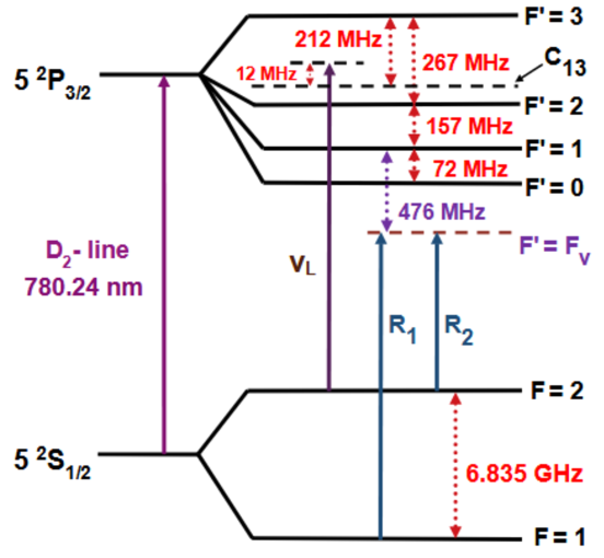
Figure 1: Relevant energy levels of ⁸⁷Rb atom for Raman transition.

The motivation for this experiment was to estimate the Rabi frequency for two-photon Raman transition, which is required for estimation of duration of $\pi$-pulse for Raman pulse atom interferometry. In the experiments, we have used linearly polarized counter-propagating Raman beams with their polarizations in mutually perpendicular directions. The Raman beams were applied on the atom cloud after $\sim$ 5 ms of the launching in vertical upward direction. An absorption probe beam, resonant to cooling transition of ⁸⁷Rb atom, was aligned horizontally at a height of $\sim$ 9 cm from the MOT center in the path of atoms moving in the upward direction. The absorption of this probe beam was recorded to know the population in $F=2$ hyperfine state after applying the Raman beams pulse. The probe absorption signal (PAS) was recorded for different values of pulse duration of the Raman beams and for three different values of total power (7.5 mW, 9.5 mW and 11.5 mW) in the Raman beams, as shown in Fig. 2. The PAS (proportional to population in $F=2$ state) shows Rabi oscillations with increase in the duration of the Raman beams, as shown in Fig. 2.

Figure 2: Rabi oscillations in atomic population in F = 2 hyperfine ground state of ⁸⁷Rb for three different total power of (a) 7.5 mW, (b) 9.5 mW and (c) 11.5 mW in Raman beams. The dashed curves (red color) are guide to eyes. PAS : Probe absorption signal.

The duration of $\pi$-pulse, i.e. the duration of Raman beams for maximum population transfer from $|5\ ^{2}S_{1/2},F=2\rangle$ to $|5\ ^{2}S_{1/2},F=1\rangle$, can be estimated from the data shown in Fig. 2. The values of $\pi$-pulse durations are $\sim$ 13 $\mu$s, $\sim$ 11 $\mu$s and $\sim$ 10 $\mu$s for the total Raman beam power of 7.5 mW, 9.5 mW and 11.5 mW respectively. It can be noted from the figure that the amplitude of the oscillations gets reduced as the pulse duration of Raman beams is increased. This damping of Rabi oscillations could be due to various decoherence mechanisms, which are investigated in the present work using a theoretical model presented in the next section.

III Theoretical Model

The two-photon Raman transition between two ground hyperfine states is a frequently used phenomenon in the atom interferometry for precision measurement [31, 32, 33]. We have modeled this Raman transition in ${}^{87}Rb$ atom by using a four-level scheme and solving the corresponding Lindblad master equation. Fig. 3 shows the schematic of the energy levels of ${}^{87}Rb$ atom involved in two-photon stimulated Raman transition between states $|5\ ^{2}S_{1/2},F=2\rangle$ and $|5\ ^{2}S_{1/2},F=1\rangle$. Two laser beams $R_{2}$ and $R_{1}$, having optical frequency $\omega_{2}$ and $\omega_{1}$ couple the two hyperfine levels $|2\rangle$ (i.e. $|5\ ^{2}S_{1/2},F=2\rangle$) and $|1\rangle$ (i.e. $|5\ ^{2}S_{1/2},F=1\rangle$) via intermediate states $|i\rangle$, with the corresponding coupling strengths $\Omega_{2i}$ and $\Omega_{i1}$ with $i=3,4$. The single-photon detuning values $\Delta_{3}$ and $\Delta_{4}$ of the Raman beams from the excited states $|3\rangle$ and $|4\rangle$, are much larger than the linewidths of the levels $|3\rangle$ and $|4\rangle$. The two-photon detuning between Raman beams and states $|1\rangle$ and $|2\rangle$ is denoted by $\delta$. The parameters $\Gamma_{ij}$ represent spontaneous emission rates and $\gamma_{ij}$ (with $i\neq j$) represent the dephasing rates between the levels (Fig. 3).

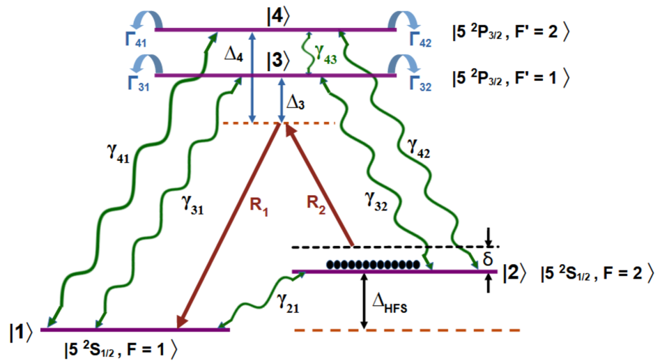
Figure 3: Schematic diagram of partial energy levels of ${}^{87}Rb$ atom for two-photon Raman transition between two states $|2\rangle$ and $|1\rangle$. $\Delta_{HFS}$ is the hyperfine energy splitting between states $|1\rangle$ and $|2\rangle$.

If atoms are initially in the state $|2\rangle$, then the stimulated Raman transition to the state $|1\rangle$ will involve absorption of a photon from one Raman beam ($R_{2}$) and the stimulated emission of a photon into the other Raman beam ($R_{1}$). For this two-photon stimulated Raman transition process, the Lindblad master equation [34, 35, 36] for evolution of the density matrix is given by,

$$\frac{d\rho}{dt}=-i[H,\rho]+L_{\text{sp}}(\rho)+L_{\text{de}}(\rho),$$ (1)

where, $\rho$ is the density matrix and H is the total Hamiltonian. $L_{sp}(\rho)$ is the Lindblad term for spontaneous emission from the excited states and $L_{de}(\rho)$ is the Lindblad term for dephasing between different levels due to various processes. The Hamiltonian for the four-level $\Lambda$-system in Fig. 3 under the interaction picture and rotating wave approximation (RWA) is given by [12, 37],

$$H=\begin{pmatrix}0&0&\frac{\Omega_{31}}{2}&\frac{\Omega_{41}}{2}\\ 0&-\delta&\frac{\Omega_{23}}{2}&\frac{\Omega_{24}}{2}\\ \frac{\Omega_{31}}{2}&\frac{\Omega_{23}}{2}&\Delta_{3}&0\\ \frac{\Omega_{41}}{2}&\frac{\Omega_{24}}{2}&0&\Delta_{4}\\ \end{pmatrix}.$$ (2)

Though the single-photon detuning $\Delta_{3}$ and $\Delta_{4}$ is large, there is still some probability of a single-photon transition, which can result in the transfer of population from the state $|2\rangle$ to $|3\rangle$ and $|4\rangle$. If the spontaneous decay rates $\Gamma_{31}$, $\Gamma_{32}$, $\Gamma_{41}$ and $\Gamma_{42}$ from the levels $|3\rangle$ and $|4\rangle$, then the Lindblad term for spontaneous emission is given by [23, 28],

$$L_{\text{sp}}(\rho)=\left(\begin{array}[]{cc}\Gamma_{31}\rho_{33}+\Gamma_{41}\rho_{44}&0\\ 0&\Gamma_{32}\rho_{33}+\Gamma_{42}\rho_{44}\\ -\frac{1}{2}(\Gamma_{31}+\Gamma_{32})\rho_{31}&-\frac{1}{2}(\Gamma_{31}+\Gamma_{32})\rho_{32}\\ -\frac{1}{2}(\Gamma_{41}+\Gamma_{42})\rho_{41}&-\frac{1}{2}(\Gamma_{41}+\Gamma_{42})\rho_{42}\\ \end{array}\right.\begin{aligned} \left.\begin{array}[]{cc}-\frac{1}{2}(\Gamma_{31}+\Gamma_{32})\rho_{13}&-\frac{1}{2}(\Gamma_{41}+\Gamma_{42})\rho_{14}\\ -\frac{1}{2}(\Gamma_{31}+\Gamma_{32})\rho_{23}&-\frac{1}{2}(\Gamma_{41}+\Gamma_{42})\rho_{24}\\ -(\Gamma_{31}+\Gamma_{32})\rho_{33}&-\frac{1}{2}(\Gamma_{31}+\Gamma_{32}+\Gamma_{41}+\Gamma_{42})\rho_{34}\\ -\frac{1}{2}(\Gamma_{31}+\Gamma_{32}+\Gamma_{41}+\Gamma_{42})\rho_{43}&-(\Gamma_{41}+\Gamma_{42})\rho_{44}\\ \end{array}\right)\end{aligned}$$ (3)

Similarly, the Lindblad term for dephasing [36, 38] between different levels can be written as,

$$L_{\text{de}}(\rho)=\begin{pmatrix}0&-\gamma_{12}\rho_{12}&-\gamma_{13}\rho_{13}&-\gamma_{14}\rho_{14}\\ -\gamma_{21}\rho_{21}&0&-\gamma_{23}\rho_{23}&-\gamma_{24}\rho_{24}\\ -\gamma_{31}\rho_{31}&-\gamma_{32}\rho_{32}&0&-\gamma_{34}\rho_{34}\\ -\gamma_{41}\rho_{41}&-\gamma_{42}\rho_{42}&-\gamma_{43}\rho_{43}&0\end{pmatrix}.$$ (4)

Using the above set of equations (Eqs.( 1)–( 4)), we have numerically solved the Lindblad equation to evaluate the time-dependent populations and coherences for different levels.

In the presence of a finite stray magnetic field in an arbitrary direction, there are several possible pathways for two-photon Raman transition from state $|F=2\rangle$ to $|F=1\rangle$ involving Zeeman sublevels of all the four hyperfine states. Each pathway for Raman transition consists of two single-photon transitions, where an atom absorbs a photon from the one Raman beam and emits a photon into the other Raman beam by stimulated emission process. The details of such Raman transition routes are given in the Appendix at the end of this paper.

Using the formalism (Eq. (A.1) and Eq. (A.2) discussed in Appendix, we can calculate the root mean square (rms) values of Rabi frequencies $\Omega_{23}$, $\Omega_{31}$, $\Omega_{24}$, and $\Omega_{41}$ for the single-photon transitions $|2\rangle\rightarrow|3\rangle$, $|3\rangle\rightarrow|1\rangle$, $|2\rangle\rightarrow|4\rangle$, and $|4\rangle\rightarrow|1\rangle$, respectively. We get the numerical values of $\Omega_{23}$, $\Omega_{31}$, $\Omega_{24}$, and $\Omega_{41}$ as $2\pi\times 3.15$ MHz, $2\pi\times 5.25$ MHz, $2\pi\times 6.58$ MHz, and $2\pi\times 4.46$ MHz, respectively. Then two-photon Rabi frequency for stimulated Raman transition $|2\rangle\rightarrow|1\rangle$ via levels $|3\rangle$ and $|4\rangle$ is given as [39, 40],

$$\Omega_{R}=\sum_{i}\frac{\Omega_{2i}\Omega_{i1}}{2\Delta_{i}},$$ (5)

where sum is over index $i$ ($i=3,4$), and $\Delta_{i}$ is the single-photon detuning of Raman beam from the intermediate level $|i\rangle$. The two-photon Rabi frequency $\Omega_{R}$ for Raman transition $|2\rangle\rightarrow|1\rangle$, as calculated for our theoretical model (using Eq.( 5)), is 2$\pi$ $\times$ 40.55 kHz. The corresponding Raman $\pi$-pulse duration is 12.33 $\mu s$.

The spontaneous emission rate $\Gamma_{F^{\prime},m^{\prime}_{F}}^{F,m_{F}}$ from the state $|F^{\prime},m^{\prime}_{F}\rangle$ to $|F,m_{F}\rangle$ is given as [41],

$$\Gamma_{F^{\prime},m^{\prime}_{F}}^{F,m_{F}}\propto\ (2J^{\prime}+1)(2F+1)(2F^{\prime}+1)\cdot\left\{\begin{array}[]{ccc}J^{\prime}&1&J\\ F&I&F^{\prime}\end{array}\right\}^{2}\cdot\left(\begin{array}[]{ccc}F^{\prime}&1&F\\ m^{\prime}_{F}&m_{F}-m^{\prime}_{F}&-m_{F}\end{array}\right)^{2}.$$ (10)

The net spontaneous emission rate ($\Gamma_{F^{\prime}F}$ ) from the state $|F^{\prime}\rangle$ to $|F\rangle$ is given as,

$$\Gamma_{F^{\prime}F}=\sum_{m_{F}^{\prime},m_{F}}\Gamma_{F^{\prime},m^{\prime}_{F}}^{F,m_{F}}\ ,$$ (11)

where sum is over all allowed transitions from all magnetic sublevels $m^{\prime}_{F}$ of the hyperfine state $F^{\prime}$ to the magnetic sublevels $m_{F}$ of the hyperfine state F. The total spontaneous emission rate from $F^{\prime}$ is given as $\Gamma=\sum_{F}\Gamma_{F^{\prime}F}$ [41]. The calculated spontaneous emission rates $\Gamma_{31}$, $\Gamma_{32}$, $\Gamma_{41}$ and $\Gamma_{42}$, in our case, are $2\pi\times 5.03$ MHz, $2\pi\times 1.03$ MHz, $2\pi\times 3.03$ MHz and $2\pi\times 3.03$ MHz, respectively.

IV Results and discussion

The theoretically calculated population in the state $|F=2\rangle$ after interaction of an atom with Raman beams for a time duration of ‘$t$’ is shown in Fig. 4. The plot in Fig. 4(a) shows the Rabi oscillations of population without any decoherence mechanisms ($L_{sp}=L_{de}=0$). The plot in Fig. 4(b) shows the effect of spontaneous emission ($L_{sp}\neq 0$ and $L_{de}=0$) from the excited states with the values of $\Gamma_{ij}$ as calculated using Eq. (11). It is noted that effect of the spontaneous emission is very weak on the Rabi oscillations, as population in the excited states ($|3\rangle$ and $|4\rangle$) remains quite small ($\sim$ $10^{-5}$ to $10^{-3}$). This can be attributed to the large detuning of Raman beams from the excited states.

Figure 4(c) shows the effect of dephasing ($L_{sp}=0$ and $L_{de}\neq 0$) on the Rabi oscillations. The dephasing parameters used in the calculation are $\gamma_{ij}=\gamma_{ji}=2\pi\times 0.1$ MHz (for $i\in\{1,2\},j\in\{3,4\}$), $\gamma_{12}=\gamma_{21}=2\pi\times 5$ kHz and $\gamma_{34}=\gamma_{43}=2\pi\times 6$ kHz. This plot shows that damping of Rabi oscillations is present due to effect of dephasing. Figure 4(d) shows the effect of spontaneous emission and dephasing both, with dephasing and spontaneous emission parameters same as in plots (c) and (b). In general, the damping of Rabi oscillations can occur due to spontaneous emission and dephasing, both, but we did not observe much contribution from the spontaneous emission (plots (b) and (d)). This is due to large detuning of Raman beams from the excited states.

Figure 4: he calculated value of population in level $|5^{2}S_{1/2},F=2\rangle$ of ${}^{87}Rb$ as function of time (t), for $\Omega_{23}=2\pi\times 3.15$ MHz, $\Omega_{31}=2\pi\times 5.25$ MHz, $\Omega_{24}=2\pi\times 6.58$ MHz, $\Omega_{41}=2\pi\times 4.46$ MHz and , $\Delta_{3}=2\pi\times 476$ MHz, $\Delta_{4}=2\pi\times 633$ MHz and $\delta=0$. The dephasing and spontaneous emission parameter are described in the text.

Next, we have compared the experimentally observed and theoretically calculated data for Rabi oscillations in two-photon Raman transition and results are as shown in Fig. 5. For the calculated graph in this figure, the same values of parameters $\Omega_{23}$, $\Omega_{31}$, $\Omega_{24}$, $\Omega_{41}$, $\Gamma_{31}$, $\Gamma_{32}$, $\Gamma_{41}$ and $\Gamma_{42}$ were used as those used in Fig. 4 corresponding to a total Raman beam power of 9.5 mW.

Figure 5: Rabi oscillations in atomic population of F = 2 hyperfine ground state of ${}^{87}{Rb}$ atom for total Raman beam power of 9.5 mW. Black open circle represent experimental data points. Solid line shows the fitted curve using theoretical model. The additional fitted parameters (except for the calculated parameters, which have been described in the text) used in this simulation are the dephasing rates: $\gamma_{ij}=\gamma_{ji}=2\pi\times 0.2$ MHz $(i\in\{1,2\}\$and$\ j\in\{3,4\}$), $\gamma_{12}=\gamma_{21}=2\pi\times 0.8$ kHz, and $\gamma_{34}=\gamma_{43}=2\pi\times 5.0$ kHz. The two-photon Raman detuning ($\delta$) is taken as $2\pi\times 15$ kHz.

From the Fig. 5, it can be noted that theory and experiments show a reasonable agreement in the values of two-photon Rabi frequency (theoretical value is 2$\pi$ $\times$ 43.24 kHz and experimental value is 2$\pi$ $\times$ 45.45 kHz). However, there is a disagreement between the theoretical and experimental data on the variation in the population amplitude. This disagreement could be due to the participation of the limited population in the Raman transition. The population of the Zeeman sublevels ($m_{F}$) that obeys only the selection rules will undergo the Raman transition. The finite value of dephasing can arise due to several factors including intensity and linewidth variation in the Raman beam, Zeeman non-degeneracy, and broadening of the detuning due to the Doppler effect. We have not quantified the contribution of each of them to the dephasing values used in the theoretical calculations.

V Conclusion

The Rabi oscillations in the population of ground hyperfine state $|5\ ^{2}S_{1/2},F=2\rangle$ of ${}^{87}Rb$ atom have been studied under a two-photon Raman excitation process. Damping in the oscillations has been experimentally observed with an increase in the interaction duration of the Raman beams with atoms. By solving the Lindblad master equation, it has been shown that damping of Rabi oscillations in two-photon Raman transition from $|5\ ^{2}S_{1/2},F=2\rangle$ to $|5\ ^{2}S_{1/2},F=1\rangle$ is dominantly due to dephasing mechanism. The decoherence due to spontaneous emission has negligible contribution to the observed damping of Rabi oscillations.

Appendix

Figure  A.1 shows two Raman beams $R_{1}$ and $R_{2}$ propagating in z-direction and having mutually orthogonal linear polarizations $\varepsilon_{x}$ and $\varepsilon_{y}$. The Raman beams interact with an atom in the presence of the stray magnetic field. Fig. A.1(a) shows the orientation of Raman beams and Fig. A.1(b) shows the various pathways for Raman transition from $|5^{2}S_{1/2},F=2\rangle$ to $|5^{2}S_{1/2},F=1\rangle$ via the intermediate state $|5^{2}P_{3/2},F^{\prime}=1\rangle$ in presence of $B_{x}$ component of the magnetic field.

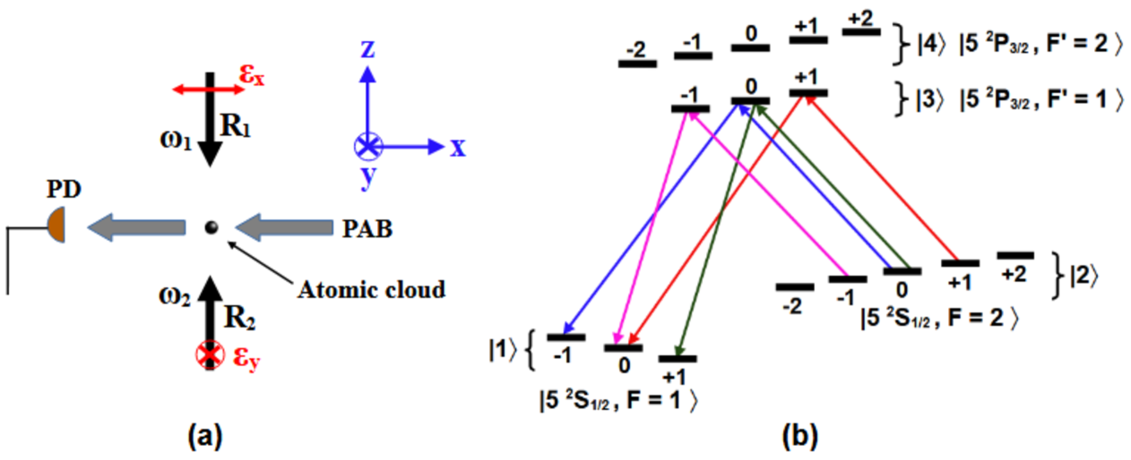
Figure A.1: (a) shows the orientation of Raman beams. (b) shows different routes for two-photon Raman transition between ground hyperfine states (from $|F=2\rangle$ to $|F=1\rangle$ ) via the intermediate state $|5^{2}P_{3/2},F^{\prime}=1\rangle$, when $B_{x}$ component of magnetic field is considered.

Since the stray magnetic field is oriented arbitrarily, each single-photon transition is governed by the direction of the polarization of the Raman beams and the direction of the stray magnetic field components ($B_{x}$, $B_{y}$, and $B_{z}$). The summary of possible single-photon transitions is given in Table A.1. Based on the direction of the magnetic field and polarization of Raman beams, the routes for Raman transitions from the state $|F=2,m_{F}\rangle$ to $|F=1,m_{F}\rangle$ via intermediate states $|F^{{}^{\prime}},m^{\prime}_{F}\rangle$, with ($F^{{}^{\prime}}=1,2$), are summarized in Table A.2.

Table A.1: Single-photon transitions in an atom interacting with a linearly polarized laser beam (propagating along the $z$-direction) in the presence of a stray magnetic field.

Magnetic Field Component	Polarization of Laser Beam	Transition Type	$\mathbf{\Delta m_{F}}$
$B_{x}$	$\varepsilon_{x}$	$\pi^{0}$	$0$
	$\varepsilon_{y}$	$\pi^{+}=\frac{(\sigma^{+}+\sigma^{-})}{\sqrt{2}}$	$\pm 1$
$B_{y}$	$\varepsilon_{x}$	$\pi^{+}=\frac{(\sigma^{+}+\sigma^{-})}{\sqrt{2}}$	$\pm 1$
	$\varepsilon_{y}$	$\pi^{0}$	$0$
$B_{z}$	$\varepsilon_{x}$	$\pi^{+}=\frac{(\sigma^{+}+\sigma^{-})}{\sqrt{2}}$	$\pm 1$
	$\varepsilon_{y}$	$\pi^{-}=\frac{(\sigma^{+}-\sigma^{-})}{\sqrt{2}}$	$\pm 1$

Table A.2: Possible routes for the transition of a ⁸⁷Rb atom from the ground hyperfine state $|F=2\rangle$ to the ground hyperfine state $|F=1\rangle$, when two Raman beams with mutually orthogonal linear polarizations ($R_{1}$ in the x-direction and $R_{2}$ in the y-direction) are used in a two-photon Raman transition in the presence of a magnetic field. Here, $F^{\prime}\ (=1,2)$ represents the hyperfine number of the intermediate level.

Magnetic Field Component	Transition Type	Two-Photon Raman Transition Routes	Via Intermediate State
$B_{x}$	$\pi^{0}-\pi^{+}$	$|2,m_{F}\rangle\rightarrow|1,m_{F}+1\rangle$	$|F^{\prime},m^{\prime}_{F}=m_{F}\rangle$
		$|2,m_{F}\rangle\rightarrow|1,m_{F}-1\rangle$	$|F^{\prime},m^{\prime}_{F}=m_{F}\rangle$
$B_{y}$	$\pi^{+}-\pi^{0}$	$|2,m_{F}\rangle\rightarrow|1,m_{F}+1\rangle$	$|F^{\prime},m^{\prime}_{F}=m_{F}+1\rangle$
		$|2,m_{F}\rangle\rightarrow|1,m_{F}-1\rangle$	$|F^{\prime},m^{\prime}_{F}=m_{F}-1\rangle$
$B_{z}$	$\pi^{+}-\pi^{-}$	$|2,m_{F}\rangle\rightarrow|1,m_{F}\rangle$	$|F^{\prime},m^{\prime}_{F}=m_{F}+1\rangle$
		$|2,m_{F}\rangle\rightarrow|1,m_{F}\rangle$	$|F^{\prime},m^{\prime}_{F}=m_{F}-1\rangle$

The Rabi frequency for a single-photon transition from the state $|J,F,m_{F}\rangle$ to $|J^{\prime},F^{\prime},m^{\prime}_{F}\rangle$, is calculated using the expression [12, 21, 42],

$$\Omega_{F,m_{F}}^{F^{\prime},m^{\prime}_{F}}= \ \frac{E}{\hbar}\times(-1)^{2F^{\prime}+I+J+m_{F}}\sqrt{(2J+1)(2F+1)(2F^{\prime}+1)}\times\begin{Bmatrix}J&J^{\prime}&1\\ F^{\prime}&F&I\end{Bmatrix}$$

$$\times\begin{pmatrix}F^{\prime}&1&F\\ m^{\prime}_{F}&m_{F}-m^{\prime}_{F}&-m_{F}\end{pmatrix}\times\langle J||e\mathbf{r}||J^{\prime}\rangle.$$ (A.1)

where, $\langle J||e\mathbf{r}||J^{\prime}\rangle$ is the reduced dipole matrix element corresponding to the transitions from the ground state $5\ ^{2}S_{1/2}$ to the excited state $5\ ^{2}P_{3/2}$ of ⁸⁷Rb atom. Here $I=3/2$ is the nuclear spin of ⁸⁷Rb atom. The symbol $\Omega_{F,m_{F}}^{F^{\prime},m^{\prime}_{F}}$ represents the Rabi frequency for the single-photon absorption for transition $|F,m_{F}\rangle\rightarrow|F^{\prime},m^{\prime}_{F}\rangle$, while the Rabi frequency $\Omega_{F^{\prime},m^{\prime}_{F}}^{F,m_{F}}$ corresponds to the single-photon stimulated emission for the $|F^{\prime},m^{\prime}_{F}\rangle\rightarrow|F,m_{F}\rangle$ transition.

The calculated values of single-photon Rabi frequencies in the $\pi^{0}-\pi^{+}$ two-photon transition routes from $|F=2,m_{F}\rangle$ to $|F=1,m_{F}\rangle$ via $|F^{\prime}=1$ or $2,m^{\prime}_{F}\rangle$ are shown in the table Table A.3 and Table A.4 for $B_{x}$ component of the stray magnetic field. Similarly, the Rabi frequencies for $\pi^{+}$ - $\pi^{0}$ transitions due to the $B_{y}$ component and the Rabi frequencies for $\pi^{+}$ - $\pi^{-}$ due to $B_{z}$ component are presented in Table A.5, Table A.6, Table A.7 and Table A.8, respectively.

Assuming a nearly the same population in each $|F,m_{F}\rangle$ state, the resultant Rabi frequency corresponding to different Rabi frequencies for different $|F,m_{F}\rangle\rightarrow|F^{\prime},m^{\prime}_{F}\rangle$ transitions can be taken as the root mean square (rms) value of these different frequencies as [26, 39, 43],

$$\Omega_{rms}=\sqrt{\frac{\sum\left(\Omega_{F,m_{F}}^{F^{\prime},m^{\prime}_{F}}\right)^{2}}{N}},$$ (A.2)

where sum is over all the different single-photon $|F,m_{F}\rangle\rightarrow|F^{\prime},m^{\prime}_{F}\rangle$ transition. Similarly, the resultant Rabi frequency for $|F^{\prime},m^{\prime}_{F}\rangle\rightarrow|F,m_{F}\rangle$ transitions can also be calculated by taking rms value.

Table A.3: Rabi frequencies for $\pi^{0}$ - $\pi^{+}$ type two-photon Raman transitions via the intermediate state $F^{\prime}=1$ for $B_{x}$ component of the stray magnetic field.

Two-photon Raman transition routes via $F^{\prime}=1$
Stimulated absorption		Stimulated emission
$|F,m_{F}\rangle$ $\rightarrow$ $|F^{\prime},m^{\prime}_{F}\rangle$	$|\Omega_{F,m_{F}}^{F^{\prime},m^{\prime}_{F}}|/2\pi$ (MHz)	$|F^{\prime},m^{\prime}_{F}\rangle$ $\rightarrow$ $|F,m_{F}\rangle$	$|\Omega_{F^{\prime},m^{\prime}_{F}}^{F,m_{F}}|/2\pi$ (MHz)
$|F=2,m_{F}=-1\rangle$ $\rightarrow$ $|F^{\prime}=1,m^{\prime}_{F}=-1\rangle$	3.15	$|F^{\prime}=1,m^{\prime}_{F}=-1\rangle$ $\rightarrow$ $|F=1,m_{F}=0\rangle$	5.25
$|F=2,m_{F}=0\rangle$ $\rightarrow$ $|F^{\prime}=1,m^{\prime}_{F}=0\rangle$	3.63	$|F^{\prime}=1,m^{\prime}_{F}=0\rangle$ $\rightarrow$ $|F=1,m_{F}=-1\rangle$	5.25
$|F=2,m_{F}=0\rangle$ $\rightarrow$ $|F^{\prime}=1,m^{\prime}_{F}=0\rangle$	3.63	$|F^{\prime}=1,m^{\prime}_{F}=0\rangle$ $\rightarrow$ $|F=1,m_{F}=1\rangle$	5.25
$|F=2,m_{F}=1\rangle$ $\rightarrow$ $|F^{\prime}=1,m^{\prime}_{F}=1\rangle$	3.15	$|F^{\prime}=1,m^{\prime}_{F}=1\rangle$ $\rightarrow$ $|F=1,m_{F}=0\rangle$	5.25

Table A.4: Rabi frequencies for $\pi^{0}$ - $\pi^{+}$ type two-photon Raman transitions via the intermediate state $F^{\prime}=2$ for $B_{x}$ component of the stray magnetic field.

Two-photon Raman transition routes via $F^{\prime}=2$
Stimulated absorption		Stimulated emission
$|F,m_{F}\rangle$ $\rightarrow$ $|F^{\prime},m^{\prime}_{F}\rangle$	$|\Omega_{F,m_{F}}^{F^{\prime},m^{\prime}_{F}}|/2\pi$ (MHz)	$|F^{\prime},m^{\prime}_{F}\rangle$ $\rightarrow$ $|F,m_{F}\rangle$	$|\Omega_{F^{\prime},m^{\prime}_{F}}^{F,m_{F}}|/2\pi$ (MHz)
$|F=2,m_{F}=-2\rangle$ $\rightarrow$ $|F^{\prime}=2,m^{\prime}_{F}=-2\rangle$	8.12	$|F^{\prime}=2,m^{\prime}_{F}=-2\rangle$ $\rightarrow$ $|F=1,m_{F}=-1\rangle$	5.75
$|F=2,m_{F}=-1\rangle$ $\rightarrow$ $|F^{\prime}=2,m^{\prime}_{F}=-1\rangle$	4.06	$|F^{\prime}=2,m^{\prime}_{F}=-1\rangle$ $\rightarrow$ $|F=1,m_{F}=0\rangle$	4.06
$|F=2,m_{F}=1\rangle$ $\rightarrow$ $|F^{\prime}=2,m^{\prime}_{F}=1\rangle$	4.06	$|F^{\prime}=2,m^{\prime}_{F}=1\rangle$ $\rightarrow$ $|F=1,m_{F}=0\rangle$	4.06
$|F=2,m_{F}=2\rangle$ $\rightarrow$ $|F^{\prime}=2,m^{\prime}_{F}=2\rangle$	8.12	$|F^{\prime}=2,m^{\prime}_{F}=2\rangle$ $\rightarrow$ $|F=1,m_{F}=1\rangle$	5.75

Table A.5: Rabi frequencies for $\pi^{+}$ - $\pi^{0}$ type two-photon Raman transitions via the intermediate state $F^{\prime}=1$ for $B_{y}$ component of the stray magnetic field.

Two-photon Raman transition routes via $F^{\prime}=2$
Stimulated absorption		Stimulated emission
$|F,m_{F}\rangle$ $\rightarrow$ $|F^{\prime},m^{\prime}_{F}\rangle$	$|\Omega_{F,m_{F}}^{F^{\prime},m^{\prime}_{F}}|/2\pi$ (MHz)	$|F^{\prime},m^{\prime}_{F}\rangle$ $\rightarrow$ $|F,m_{F}\rangle$	$|\Omega_{F^{\prime},m^{\prime}_{F}}^{F,m_{F}}|/2\pi$ (MHz)
$|F=2,m_{F}=-2\rangle$ $\rightarrow$ $|F^{\prime}=1,m^{\prime}_{F}=-1\rangle$	4.45	$|F^{\prime}=1,m^{\prime}_{F}=-1\rangle$ $\rightarrow$ $|F=1,m_{F}=-1\rangle$	5.25
$|F=2,m_{F}=0\rangle$ $\rightarrow$ $|F^{\prime}=1,m^{\prime}_{F}=-1\rangle$	1.82	$|F^{\prime}=1,m^{\prime}_{F}=-1\rangle$ $\rightarrow$ $|F=1,m_{F}=-1\rangle$	5.25
$|F=2,m_{F}=0\rangle$ $\rightarrow$ $|F^{\prime}=1,m^{\prime}_{F}=1\rangle$	1.82	$|F^{\prime}=1,m^{\prime}_{F}=1\rangle$ $\rightarrow$ $|F=1,m_{F}=1\rangle$	5.25
$|F=2,m_{F}=2\rangle$ $\rightarrow$ $|F^{\prime}=1,m^{\prime}_{F}=1\rangle$	4.45	$|F^{\prime}=1,m^{\prime}_{F}=1\rangle$ $\rightarrow$ $|F=1,m_{F}=1\rangle$	5.25

Table A.6: Rabi frequencies for $\pi^{+}$ - $\pi^{0}$ type two-photon Raman transitions via the intermediate state $F^{\prime}=2$ for $B_{y}$ component of the stray magnetic field.

Two-photon Raman transition routes via $F^{\prime}=2$
Stimulated absorption		Stimulated emission
$|F,m_{F}\rangle$ $\rightarrow$ $|F^{\prime},m^{\prime}_{F}\rangle$	$|\Omega_{F,m_{F}}^{F^{\prime},m^{\prime}_{F}}|/2\pi$ (MHz)	$|F^{\prime},m^{\prime}_{F}\rangle$ $\rightarrow$ $|F,m_{F}\rangle$	$|\Omega_{F^{\prime},m^{\prime}_{F}}^{F,m_{F}}|/2\pi$ (MHz)
$|F=2,m_{F}=-2\rangle$ $\rightarrow$ $|F^{\prime}=2,m^{\prime}_{F}=-1\rangle$	5.75	$|F^{\prime}=2,m^{\prime}_{F}=-1\rangle$ $\rightarrow$ $|F=1,m_{F}=-1\rangle$	4.06
$|F=2,m_{F}=-1\rangle$ $\rightarrow$ $|F^{\prime}=2,m^{\prime}_{F}=0\rangle$	7.04	$|F^{\prime}=2,m^{\prime}_{F}=0\rangle$ $\rightarrow$ $|F=1,m_{F}=0\rangle$	4.69
$|F=2,m_{F}=0\rangle$ $\rightarrow$ $|F^{\prime}=2,m^{\prime}_{F}=-1\rangle$	7.04	$|F^{\prime}=2,m^{\prime}_{F}=-1\rangle$ $\rightarrow$ $|F=1,m_{F}=-1\rangle$	4.06
$|F=2,m_{F}=0\rangle$ $\rightarrow$ $|F^{\prime}=2,m^{\prime}_{F}=1\rangle$	7.04	$|F^{\prime}=2,m^{\prime}_{F}=1\rangle$ $\rightarrow$ $|F=1,m_{F}=1\rangle$	4.06
$|F=2,m_{F}=1\rangle$ $\rightarrow$ $|F^{\prime}=2,m^{\prime}_{F}=0\rangle$	7.04	$|F^{\prime}=2,m^{\prime}_{F}=0\rangle$ $\rightarrow$ $|F=1,m_{F}=0\rangle$	4.69
$|F=2,m_{F}=2\rangle$ $\rightarrow$ $|F^{\prime}=2,m^{\prime}_{F}=1\rangle$	5.75	$|F^{\prime}=2,m^{\prime}_{F}=1\rangle$ $\rightarrow$ $|F=1,m_{F}=1\rangle$	4.06

Table A.7: Rabi frequencies for $\pi^{+}$ - $\pi^{-}$ type two-photon Raman transitions via the intermediate state $F^{\prime}=1$ for $B_{z}$ component of the stray magnetic field.

Two-photon Raman transition routes via $F^{\prime}=1$
Stimulated absorption		Stimulated emission
$|F,m_{F}\rangle$ $\rightarrow$ $|F^{\prime},m^{\prime}_{F}\rangle$	$|\Omega_{F,m_{F}}^{F^{\prime},m^{\prime}_{F}}|/2\pi$ (MHz)	$|F^{\prime},m^{\prime}_{F}\rangle$ $\rightarrow$ $|F,m_{F}\rangle$	$|\Omega_{F^{\prime},m^{\prime}_{F}}^{F,m_{F}}|/2\pi$ (MHz)
$|F=2,m_{F}=-1\rangle$ $\rightarrow$ $|F^{\prime}=1,m^{\prime}_{F}=0\rangle$	3.15	$|F^{\prime}=1,m^{\prime}_{F}=0\rangle$ $\rightarrow$ $|F=1,m_{F}=-1\rangle$	5.25
$|F=2,m_{F}=0\rangle$ $\rightarrow$ $|F^{\prime}=1,m^{\prime}_{F}=-1\rangle$	1.82	$|F^{\prime}=1,m^{\prime}_{F}=-1\rangle$ $\rightarrow$ $|F=1,m_{F}=0\rangle$	5.25
$|F=2,m_{F}=0\rangle$ $\rightarrow$ $|F^{\prime}=1,m^{\prime}_{F}=+1\rangle$	1.82	$|F^{\prime}=1,m^{\prime}_{F}=+1\rangle$ $\rightarrow$ $|F=1,m_{F}=0\rangle$	5.25
$|F=2,m_{F}=1\rangle$ $\rightarrow$ $|F^{\prime}=1,m^{\prime}_{F}=0\rangle$	3.15	$|F^{\prime}=1,m^{\prime}_{F}=0\rangle$ $\rightarrow$ $|F=1,m_{F}=1\rangle$	5.25

Table A.8: Rabi frequencies for $\pi^{+}$ - $\pi^{-}$ type two-photon Raman transitions via the intermediate state $F^{\prime}=2$ for $B_{z}$ component of the stray magnetic field.

Two-photon Raman transition routes via $F^{\prime}=2$
Stimulated absorption		Stimulated emission
$|F,m_{F}\rangle$ $\rightarrow$ $|F^{\prime},m^{\prime}_{F}\rangle$	$|\Omega_{F,m_{F}}^{F^{\prime},m^{\prime}_{F}}|/2\pi$ (MHz)	$|F^{\prime},m^{\prime}_{F}\rangle$ $\rightarrow$ $|F,m_{F}\rangle$	$|\Omega_{F^{\prime},m^{\prime}_{F}}^{F,m_{F}}|/2\pi$ (MHz)
$|F=2,m_{F}=-1\rangle$ $\rightarrow$ $|F^{\prime}=2,m^{\prime}_{F}=-2\rangle$	5.75	$|F^{\prime}=2,m^{\prime}_{F}=-2\rangle$ $\rightarrow$ $|F=1,m_{F}=-1\rangle$	5.75
$|F=2,m_{F}=-1\rangle$ $\rightarrow$ $|F^{\prime}=2,m^{\prime}_{F}=0\rangle$	7.04	$|F^{\prime}=2,m^{\prime}_{F}=0\rangle$ $\rightarrow$ $|F=1,m_{F}=-1\rangle$	2.34
$|F=2,m_{F}=0\rangle$ $\rightarrow$ $|F^{\prime}=2,m^{\prime}_{F}=-1\rangle$	7.04	$|F^{\prime}=2,m^{\prime}_{F}=-1\rangle$ $\rightarrow$ $|F=1,m_{F}=0\rangle$	4.06
$|F=2,m_{F}=0\rangle$ $\rightarrow$ $|F^{\prime}=2,m^{\prime}_{F}=1\rangle$	7.04	$|F^{\prime}=2,m^{\prime}_{F}=1\rangle$ $\rightarrow$ $|F=1,m_{F}=0\rangle$	4.06
$|F=2,m_{F}=1\rangle$ $\rightarrow$ $|F^{\prime}=2,m^{\prime}_{F}=0\rangle$	7.04	$|F^{\prime}=2,m^{\prime}_{F}=0\rangle$ $\rightarrow$ $|F=1,m_{F}=1\rangle$	2.34
$|F=2,m_{F}=1\rangle$ $\rightarrow$ $|F^{\prime}=2,m^{\prime}_{F}=2\rangle$	5.75	$|F^{\prime}=2,m^{\prime}_{F}=2\rangle$ $\rightarrow$ $|F=1,m_{F}=1\rangle$	5.75

References

- Kosugi et al. [2005] N. Kosugi, S. Matsuo, K. Konno, and N. Hatakenaka, Theory of damped Rabi oscillations, Phys. Rev. B Condens. Matter 72, 172509 (2005).
- Foot [2005] C. J. Foot, Atomic physics, Vol. 7 (Oxford University Press, 2005).
- Nielsen and Chuang [2010] M. A. Nielsen and I. L. Chuang, Quantum computation and quantum information (Cambridge University Press, 2010).
- Qiao and Jiayin [2015] B. Qiao and G. Jiayin, The Rabi oscillation in subdynamic system for quantum computing, Adv. math. phys. 2015, 151690 (2015).
- Rosi et al. [2014] G. Rosi, F. Sorrentino, L. Cacciapuoti, M. Prevedelli, and G. M. Tino, Precision measurement of the Newtonian gravitational constant using cold atoms, Nature 510, 518 (2014).
- Peters et al. [2001] A. Peters, K. Y. Chung, and S. Chu, High-precision gravity measurements using atom interferometry, Metrologia 38, 25 (2001).
- Scully and Zubairy [1997] M. O. Scully and M. S. Zubairy, Quantum optics (Cambridge University Press, 1997).
- Gerry and Knight [2023] C. C. Gerry and P. L. Knight, Introductory quantum optics (Cambridge University Press, 2023).
- Berrada [2013] K. Berrada, Investigation of quantum and classical correlations in a quantum dot system under decoherence, Laser Physics 23, 095201 (2013).
- Busch et al. [2007] T. Busch, K. Deasy, and S. N. Chormaic, Quantum state preparation using multi-level-atom optics, in J. Phys. Conf. Ser., Vol. 84 (IOP Publishing, 2007) p. 012002.
- Sargent III and Horwitz [1976] M. Sargent III and P. Horwitz, Three-level Rabi flopping, Phys. Rev. A 13, 1962 (1976).
- Bateman et al. [2010] J. Bateman, A. Xuereb, and T. Freegarde, Stimulated Raman transitions via multiple atomic levels, Phys. Rev. A 81, 043808 (2010).
- Bernard et al. [2022] J. Bernard, Y. Bidel, M. Cadoret, C. Salducci, N. Zahzam, S. Schwartz, A. Bonnin, C. Blanchard, and A. Bresson, Atom interferometry using - Raman transitions between and , Phys. Rev. A 105, 033318 (2022).
- Johnson et al. [2008] T. A. Johnson, E. Urban, T. Henage, L. Isenhower, D. D. Yavuz, T. G. Walker, and M. Saffman, Rabi oscillations between ground and Rydberg states with dipole-dipole atomic interactions, Phys. Rev. Lett. 100, 113003 (2008).
- De Léséleuc et al. [2018] S. De Léséleuc, D. Barredo, V. Lienhard, A. Browaeys, and T. Lahaye, Analysis of imperfections in the coherent optical excitation of single atoms to rydberg states, Phys. Rev. A 97, 053803 (2018).
- Camparo and Coffer [1999] J. C. Camparo and J. G. Coffer, Conversion of laser phase noise to amplitude noise in a resonant atomic vapor: The role of laser linewidth, Phys. Rev. A 59, 728 (1999).
- Schneider and Milburn [1998] S. Schneider and G. J. Milburn, Decoherence in ion traps due to laser intensity and phase fluctuations, Phys. Rev. A 57, 3748 (1998).
- Brouard and Plata [2004] S. Brouard and J. Plata, Decoherence of trapped-ion internal and vibrational modes: The effect of fluctuating magnetic fields, Phys. Rev. A 70, 013413 (2004).
- Hu et al. [2017] Q. Q. Hu, Y. K. Luo, A. A. Jia, C. H. Wei, S.-H. Yan, and J. Yang, Scheme for suppressing atom expansion induced contrast loss in atom interferometers, Opt. Commun. 390, 111 (2017).
- Mielec et al. [2018] N. Mielec, M. Altorio, R. Sapam, D. Horville, D. Holleville, L. A. Sidorenkov, A. Landragin, and R. Geiger, Atom interferometry with top-hat laser beams, Appl. Phys. Lett. 113 (2018).
- G. Christandl et al. [2016] K. G. Christandl, G. D. Gillen, M. J. Piotrowicz, and M. Saffman, Comparison of Gaussian and super Gaussian laser beams for addressing atomic qubits, Appl. Phys. B 122, 1 (2016).
- Lee and Lee [2006] S. K. Lee and H. W. Lee, Damped population oscillation in a spontaneously decaying two-level atom coupled to a monochromatic field, Phys. Rev. A 74, 063817 (2006).
- Ivanov et al. [2005] P. A. Ivanov, N. V. Vitanov, and K. Bergmann, Spontaneous emission in stimulated Raman adiabatic passage, Phys. Rev. A 72, 053412 (2005).
- Abdalla et al. [2013] M. S. Abdalla, A. S. F. Obada, E. M. Khalil, and S. I. Ali, The influence of phase damping on a two-level atom in the presence of the classical laser field, Laser Physics 23, 115201 (2013).
- Kuhr et al. [2005] S. Kuhr, W. Alt, D. Schrader, I. Dotsenko, Y. Miroshnychenko, A. Rauschenbeutel, and D. Meschede, Analysis of dephasing mechanisms in a standing-wave dipole trap, Phys. Rev. A 72, 023406 (2005).
- Shore [1991] B. Shore, The theory of coherent atomic excitation (1991).
- Fox [2006] M. Fox, Quantum optics: An introduction, Vol. 15 (Oxford University Press, 2006).
- Shi and Zhao [2021a] X. Shi and H. Q. Zhao, Effect of spontaneous emission on the shortcut to adiabaticity in three-state systems, Phys. Rev. A 104, 052221 (2021a).
- Zhao and Cui [2019] Y. Zhao and B. Cui, Dissipative dynamics of cold atoms in an optical lattice, Laser Physics 29, 115501 (2019).
- Singh et al. [2021] S. Singh, B. Jain, S. P. Ram, V. B. Tiwari, and S. R. Mishra, A single laser-operated magneto-optical trap for Rb atomic fountain, Pramana 95, 1 (2021).
- Lellouch et al. [2022] S. Lellouch, K. Bongs, and M. Holynski, Using atom interferometry to measure gravity, Contemp. Phys. 63, 138 (2022).
- Zhou et al. [2011] L. Zhou, Z. Y. Xiong, W. Yang, B. Tang, W. C. Peng, Y.-B. Wang, P. Xu, J. Wang, and M. S. Zhan, Measurement of local gravity via a cold atom interferometer, Chin. Phys. Lett. 28, 013701 (2011).
- Moler et al. [1992] K. Moler, D. S. Weiss, M. Kasevich, and S. Chu, Theoretical analysis of velocity-selective Raman transitions, Phys. Rev. A 45, 342 (1992).
- Willette et al. [2011] T. Z. Willette, E. de Clercq, and E. Arimondo, Ultrahigh-resolution spectroscopy with atomic or molecular dark resonances: Exact steady-state line shapes and asymptotic profiles in the adiabatic pulsed regime, Phys. Rev. A 84, 062502 (2011).
- Shi and Zhao [2021b] X. Shi and H. Q. Zhao, Effect of spontaneous emission on the shortcut to adiabaticity in three-state systems, Phys. Rev. A 104, 052221 (2021b).
- Ivanov et al. [2004] P. A. Ivanov, N. V. Vitanov, and K. Bergmann, Effect of dephasing on stimulated Raman adiabatic passage, Phys. Rev. A 70, 063409 (2004).
- Kok and Lovett [2010] P. Kok and B. W. Lovett, Introduction to optical quantum information processing (Cambridge University Press, 2010).
- Lazarou and Vitanov [2010] C. Lazarou and N. V. Vitanov, Dephasing effects on stimulated raman adiabatic passage in tripod configurations, Phys. Rev. A 82, 033437 (2010).
- Dunning [2015] A. J. Dunning, Coherent atomic manipulation and cooling (Springer, 2015).
- Kasevich and Chu [1992] M. Kasevich and S. Chu, Measurement of the gravitational acceleration of an atom with a light-pulse atom interferometer, Appl. Phys. B: Lasers Opt. 54, 321 (1992).
- Salvi et al. [2023] L. Salvi, L. Cacciapuoti, G. M. Tino, and G. Rosi, Atom interferometry with Rb blue transitions, Phys. Rev. Lett. 131, 103401 (2023).
- Steck [2003] D. A. Steck, Rubidium 87 D-line data (2003).
- Shore [1978] B. W. Shore, Effects of magnetic sublevel degeneracy on Rabi oscillations, Phys. Rev. A 17, 1739 (1978).