Onsager-Machlup Functional and Large Deviation Principle for Stochastic Hamiltonian Systems

Abstract.

This paper investigates the application of KAM theory within the probabilistic framework of stochastic Hamiltonian systems. We begin by deriving the Onsager-Machlup functional for the stochastic Hamiltonian system, identifying the most probable transition path for system trajectories. By establishing a large deviation principle for the system, we derive a rate function that quantifies the system’s deviation from the most probable path, particularly in the context of rare events. Furthermore, leveraging classical KAM theory, we demonstrate that invariant tori remain stable, in the most probable sense, despite small random perturbations. Notably, we establish that the exponential decay rate for deviations from these persistent tori coincides precisely with the previously derived rate function, providing a quantitative probabilistic characterization of quasi-periodic motions in stochastic settings.

1. Introduction

This paper focuses on the persistence of invariant tori in stochastic Hamiltonian systems, particularly examining their stability under random perturbations. We consider the following stochastic Hamiltonian system:

(1.1) $$\begin{cases}\,{\rm d}q(t)=\frac{\partial H}{\partial p}(q(t),p(t))\,{\rm d}t+\sigma_{q}(t)\,{\rm d}W_{q}(t),\\ \,{\rm d}p(t)=-\frac{\partial H}{\partial q}(q(t),p(t))\,{\rm d}t+\sigma_{p}(t)\,{\rm d}W_{p}(t),\end{cases}$$

where $H(q,p)$ is the Hamiltonian, $\sigma_{q}(t)$ and $\sigma_{p}(t)$ represent the strengths of the random perturbations, and $W_{q}(t)$ and $W_{p}(t)$ are standard Wiener processes. By integrating the Onsager-Machlup functional, large deviation principles and KAM theory, we establish a framework for analyzing the most probable paths and stability of the system under stochastic conditions, thereby revealing the persistence of invariant tori in the most probable context.

Hamiltonian systems are foundational in classical mechanics, with applications across physics, astronomy, mechanical systems, and more. The core framework, dating back to the early 19th century, was introduced by William Rowan Hamilton. Hamiltonian mechanics describes a system’s state via generalized coordinates $q$ and conjugate momenta $p$, while the Hamiltonian function $H(q,p)$ represents the system’s total energy, encompassing both kinetic and potential energy. The evolution of such a system is governed by the Hamiltonian equations:

$$\begin{cases}\,{\rm d}q(t)=\frac{\partial H}{\partial p}(q(t),p(t))\,{\rm d}t,\\ \,{\rm d}p(t)=-\frac{\partial H}{\partial q}(q(t),p(t))\,{\rm d}t.\end{cases}$$

This formulation not only provides a precise description of system dynamics but also ensures energy conservation and preservation of symplectic geometry. However, when subjected to perturbations, the system’s behavior can become complex. In particular, understanding how to maintain long-term stability under small perturbations presents a critical challenge.

To address these challenges, the KAM theory was a significant breakthrough in the 20th century. Kolmogorov [25] hypothesized that when Hamiltonian systems are subject to small perturbations, some of the invariant tori (regular orbital structures) would persist and avoid chaotic behavior. Arnold [1] and Moser [33] subsequently provided rigorous proofs of this conjecture, formalizing what is now known as the KAM theory. The core result demonstrates that under small perturbations, most of invariant tori continue to exist, preserving the system’s quasi-periodic motions. This result profoundly advanced the study of Hamiltonian systems’ stability under perturbations. Subsequent relevant developments are referred to as [19, 36, 26, 35, 30, 6, 9, 37], and so on.

The original KAM framework was designed primarily for deterministic perturbations, leaving the question of its applicability in stochastic settings unresolved. As a result, validating the extension of the KAM theory under stochastic perturbations and quantifying the stability of invariant tori has emerged as a central problem in stochastic Hamiltonian system research. Recent studies have made significant progress in this area. Wu [44] established a framework for both large and moderate deviations in stochastic Hamiltonian systems, providing a quantitative assessment of the probability of rare events. Talay [42] explored how stochastic Hamiltonian systems asymptotically converge to an invariant measure, with a focus on the exponential nature of this convergence. Lázaro-Camí and Ortega [27] investigated the impact of stochastic noise on classical Hamiltonian dynamics, elucidating how structural preservation can be described in stochastic environments. Zhang [45] examined stochastic flows within Hamiltonian systems and introduced new computational methods based on the Bismut formula. Li [29] proposed an averaging principle framework for completely integrable stochastic Hamiltonian systems, simplifying the analysis of their long-term behavior under small stochastic perturbations. Some of the latest research references are [11, 12, 8] and so on.

The value of this paper lies in its novel analytical framework for understanding the stability of invariant tori in stochastic Hamiltonian systems. By integrating the Onsager-Machlup functional, large deviation theory, and KAM theory, we provide new insights into how these systems behave under stochastic perturbations.

The Onsager-Machlup functional is a key analytical tool for studying path probabilities and rare events. It identifies the most probable transition paths among all smooth paths in a noise-driven system. This functional quantifies the likelihood of different paths in a probabilistic setting, playing a role similar to the action functional in classical mechanics. The Onsager-Machlup functional originated from the work of Onsager [34] and Machlup [31] in 1953, where it was introduced to describe the probability density functional for diffusion processes with linear drift and constant diffusion coefficients. Subsequently, in 1957, Tisza and Manning [43] extended its application to nonlinear equations, and in the same year, Stratonovich [40] provided a rigorous theoretical framework. Recent developments refer to [32, 3, 5, 28, 4], and so on. In stochastic Hamiltonian systems, the Onsager-Machlup functional is a powerful tool for identifying the most probable path under random perturbations, and it provides a foundation for further large deviation analysis.

The origins of large deviation theory and its associated research can be traced back to the early 20th century. Cramér [10] and Sanov [39] made foundational contributions to the study of large deviations in sequences of independent and identically distributed random variables. Subsequently, Donsker and Varadhan [15, 16, 17] systematically studied large deviations in the context of Markov processes and their connection to ergodicity. Their work introduced key concepts such as Varadhan’s integral lemma and the contraction principle, which are not only central results in large deviation theory but also established deep connections with other fields of mathematics (see [41, 13, 14, 20]). In the 1970s, Freidlin and Wentzell [21] extended the theory by applying it to stochastic dynamical systems and stochastic differential equations, particularly in the context of small perturbations. The Freidlin-Wentzell framework describes the probability of a system deviating from its most likely path and introduces the rate function to quantify the distribution of deviations from typical behavior. In our consideration, this rate function, derived from extremal analysis of the Onsager-Machlup functional, allows for effective prediction of the probability distribution of deviations from invariant tori. This provides a novel perspective for quantifying system stability under stochastic perturbations and is of significant importance for understanding the long-term stability of stochastic Hamiltonian systems.

We begin by calculating the Onsager-Machlup functional for stochastic Hamiltonian systems. Due to Hamiltonian system’s symplectic structure, we show that its Onsager-Machlup functional is given by:

$$\quad OM(\varphi_{q},\varphi_{p})$$

$$=\int_{0}^{1}\left\|\sigma_{q}^{-1}(t)\left(\dot{\varphi}_{q}-\frac{\partial H}{\partial\varphi_{p}}(\varphi_{q},\varphi_{p})\right)\right\|^{2}\,{\rm d}t+\int_{0}^{1}\left\|\sigma_{p}^{-1}(t)\left(\dot{\varphi}_{p}+\frac{\partial H}{\partial\varphi_{q}}(\varphi_{q},\varphi_{p})\right)\right\|^{2}\,{\rm d}t.$$

Next, we minimize the Onsager-Machlup functional using the Euler-Lagrange equations to determine the most probable continuous path. We demonstrate that this most probable path corresponds to the solution of the deterministic Hamiltonian system without stochastic perturbations. By combining the Onsager-Machlup functional with the Freidlin-Wentzell large deviation theory [28], we establish the large deviation principle for the stochastic Hamiltonian system. Furthermore, we derive the rate function of the system, which quantifies the deviation between rare paths and the most probable path. Finally, leveraging classical KAM theory, we prove that for a nearly integrable Hamiltonian system, the invariant tori remain stable in the most probable sense even under small stochastic perturbations, provided that the system satisfies the non-degeneracy and Diophantine conditions. Importantly, we find that the probability of deviation from these invariant tori can be characterized by the rate function derived earlier.

The structure of this paper is as follows: In Section 2, we review some basic definitions of spaces and norms, introduce the concept of the Onsager-Machlup functional, and present several key technical lemmas. In Section 3, we derive the Onsager-Machlup functional for stochastic Hamiltonian systems. In Section 4, we prove that the most probable path of a stochastic Hamiltonian system corresponds to the stable solution of its associated deterministic Hamiltonian system. A specific example of a one-dimensional stochastic harmonic oscillator is provided to illustrate our results. In Section 5, we derive the large deviation principle for stochastic Hamiltonian systems. Finally, in Section 6, we extend the preceding results to the case of nearly integrable stochastic Hamiltonian systems, proving a stochastic version of the KAM theory and providing specific examples to illustrate our findings.

2. Preliminaries

2.1. Approximate limits in Wiener space

In this section, we recall some fundamental definitions and results concerning approximate limits in Wiener space. Specifically, we focus on the measurable semi-norm, which pertains to the exponentials of random variables in the first and second Wiener chaos (reference [42]).

Let $W=\left\{W_{t},~t\in[0,1]\right\}$ be a Brownian motion (Wiener process) defined in the complete filtered probability space $(\Omega,\mathcal{F},\left\{\mathcal{F}_{t}\right\}_{t\geq 0},\mathbb{P})$. Here, $\Omega$ represents the space of continuous functions vanishing at zero, and $\mathbb{P}$ denotes the Wiener measure. Let $\mathbb{H}:=L^{2}([0,1],\mathbb{R}^{n})$ be a Hilbert space and $\mathbb{H}^{1}$ be the Cameron-Martin space defined as follows:

$$\mathbb{H}^{1} :=\left\{f:[0,1]\to\mathbb{R}^{n}\in\mathbb{H}^{1}~\big{|}~f(0)=0,f~\text{is absolutely continuous functions}\right.$$

$$\qquad\left.\text{and}~f^{\prime}\in\mathbb{H}\right\}.$$

The scalar product in $\mathbb{H}^{1}$ is defined as follows:

$$\langle f,g\rangle_{\mathbb{H}^{1}}=\langle f^{\prime},g^{\prime}\rangle_{\mathbb{H}}$$

for all $f,g\in\mathbb{H}^{1}$. Let $\mathcal{P}:\mathbb{H}^{1}\to\mathbb{H}^{1}$ be an orthogonal projection with $dim\mathcal{P}\mathbb{H}^{1}<\infty$ and the specific expression

$$\mathcal{P}h=\sum_{i=1}^{n}\langle h_{i},f\rangle h_{i},$$

where $(h_{1},...,h_{n})$ is a set of orthonormal basis in $\mathcal{P}\mathbb{H}^{1}$. In addition, we can also define the $\mathbb{H}^{1}$-valued random variable

$$\mathcal{P}^{W}=\sum_{i=1}^{n}\bigg{(}\int_{0}^{1}{h_{i}^{\prime}}\,{\rm d}W_{s}\bigg{)}h_{i},$$

where $\mathcal{P}^{W}$ does not depend on $(h_{1},...,h_{n})$.

Definition 2.1.

We say that a sequence of orthogonal projections $\mathcal{P}_{n}$ on $\mathbb{H}^{1}$ is an approximating sequence of projections, if $dim\mathcal{P}_{n}\mathbb{H}^{1}<\infty$ and $\mathcal{P}_{n}$ converges strongly to the identity operator $I$ in $\mathbb{H}^{1}$ as $n\to\infty$.

Definition 2.2.

We say that a semi-norm $\mathcal{N}$ on $\mathbb{H}^{1}$ is measurable, if there exists a random variable $\tilde{\mathcal{N}}$, satisfying $\tilde{\mathcal{N}}<\infty$ a.s, such that for any approximating sequence of projections $\mathcal{P}_{n}$ on $\mathbb{H}^{1}$, the sequence $\mathcal{N}(\mathcal{P}^{W}_{n})$ converges to $\tilde{\mathcal{N}}$ in probability and $\mathbb{P}(\tilde{\mathcal{N}}\leq\epsilon)>0$ for any $\epsilon>0$. Moreover, if $\mathcal{N}$ is a norm on $\mathbb{H}^{1}$, then we call it a measurable norm.

For proving the measurability of the semi-norm defined in this paper, it is necessary to introduce the following lemma (see [22]).

Lemma 2.3.

Let $\mathcal{N}_{n}$ be a nondecreasing sequence of measurable semi-norms. Suppose that $\tilde{\mathcal{N}}:=\mathbb{P}\text{-}\!\lim\limits_{n\to\infty}\tilde{\mathcal{N}}_{n}$ exists and $\mathbb{P}(\tilde{\mathcal{N}}\leq\epsilon)>0$ for any $\epsilon>0$. In addition, if the limit $\lim\limits_{n\to\infty}\mathcal{N}_{n}$ exists on $\mathbb{H}^{1}$, then $\mathcal{N}:=\lim\limits_{n\to\infty}\mathcal{N}_{n}$ is a measurable semi-norm.

Definition 2.4.

Let $f$ be a function defined on $\Omega$. For $0<\alpha<1$, we introduce Hölder norm ($\alpha$-Hölder)

$$\|f\|_{\alpha;\Omega}=\|f\|_{0;\Omega}+\left[f\right]_{\alpha;\Omega},$$

where $\|f\|_{0;\Omega}$ represents the supremum norm of $f$ on $\Omega$, and $\left[f\right]_{\alpha;\Omega}$ represents the Hölder semi-norm of $f$ on $\Omega$. The specific expression is as follows:

$$\|f\|_{0;\Omega}=\sup\limits_{x\in\Omega}|f(x)|,\quad\left[f\right]_{\alpha;\Omega}=\sup\limits_{x,y\in\Omega,x\neq y}\frac{\left|f(x)-f(y)\right|}{|x-y|^{\alpha}}.$$

Throughout this paper, if not mentioned otherwise, norm $\|\cdot\|$ denotes Hölder norm $\|\cdot\|_{\alpha}$.

2.2. Onsager-Machlup functional

In the problem of finding the most probable path of a diffusion process, the probability of a single path is zero. Instead, we can search for the probability that the path lies within a certain region, which could be a tube along a differentiable function. This tube is defined as

$$K(\varphi,\epsilon)=\{x-x_{0}\in\mathbb{H}^{1}\mid\varphi-x_{0}\in\mathbb{H}^{1},\|x-\varphi\|\leq\epsilon,\epsilon>0\}.$$

Once $\epsilon>0$ is given, the probability of the tube can be expressed as

$$\mu_{x}(K(\varphi,\epsilon))=P\left(\{\omega\in\Omega\mid X_{t}(\omega)\in K(\varphi,\epsilon)\}\right),$$

allowing us to compare the probabilities of the tubes for all $\varphi-x_{0}\in\mathbb{H}^{1}$.

Thus, the Onsager-Machlup function can be defined as the Lagrangian function that gives the most probable tube. We now introduce the definitions of the Onsager-Machlup function and the Onsager-Machlup functional.

Definition 2.5.

Consider a tube surrounding a reference path $\varphi_{t}$ with initial value $\varphi_{0}=x$ and $\varphi_{t}-x$ belongs to $\mathbb{H}^{1}$. Assuming $\epsilon$ is given and small enough, we estimate the probability that the solution process $X_{t}$ is located in that tube as:

$$\mathbb{P}\left\{\|X-\varphi\|\leq\epsilon\right\}\propto C(\epsilon){\rm exp}\left\{-\frac{1}{2}\int_{0}^{1}{OM(t,\varphi,\dot{\varphi})}\,{\rm d}t\right\},$$

where $\propto$ denotes the equivalence relation for $\epsilon$ small enough. We call the integrand $OM(t,\varphi,\dot{\varphi})$ the Onsager-Machulup function and also call integral $\int_{0}^{1}{OM(t,\varphi,\dot{\varphi})}\,{\rm d}t$ the Onsager-Machulup functional. In analogy to classical mechanics, we also refer to the Onsager-Machulup function as the Lagrangian function and the Onsager-Machulup functional as the action functional.

2.3. KAM Theory

In Hamiltonian mechanics, invariant tori describe the set of solutions exhibiting quasi-periodic motion. These tori are higher-dimensional analogs of closed orbits, which arise when the system evolves with incommensurate frequencies. Systems with invariant tori are often referred to as integrable systems, as their dynamics are regular, confined to these tori, and predictable in phase space.

KAM theory focuses on investigating the stability of these invariant tori under small perturbations. For a nearly integrable Hamiltonian system, where the Hamiltonian is composed of an integrable part plus a small perturbation term, KAM theory asserts that as long as the perturbation is sufficiently small and certain conditions are met, most of the original invariant tori persist, albeit with slight deformations.

We cite the following theorem from [26]:

Theorem 2.6 (Koudjinan).

Consider a Hamiltonian of the form $H(I,\theta)=K(I)+P(I,\theta)$, where $I\in\mathcal{D}\subset\mathbb{R}^{d}$ are the action variables and $\theta\in\mathbb{T}^{d}$ are the angle variables. Here, $K(I)$ and $P(I,\theta)$ are $C^{l}$-smooth functions with $K,P\in C^{l}(\mathcal{D}\times\mathbb{T}^{d})$, where $\mathcal{D}$ is a non-empty bounded domain in $\mathbb{R}^{d}$. If $K$ is non-degenerate and $l>2\nu>2d$, then all the KAM tori of the integrable system $K$ whose frequency are $(\alpha,\tau)$-Diophantine, with $\alpha\simeq\epsilon^{1/2-\nu/l}$ and $\tau:=\nu-1$, do survive, being only slightly deformed, where $\epsilon$ is the $C^{l}$-norm of the perturbation $P$. Moreover, letting $\mathcal{K}$ be the corresponding family of KAM tori of $H$, we have

$$\mathrm{meas}(\mathcal{D}\times\mathbb{T}^{d}\setminus\mathcal{K})=O(\epsilon^{1/2-\nu/l}).$$

This theorem provides a more refined theoretical foundation for the persistence of invariant tori in finitely differentiable Hamiltonian systems, extending the classical KAM theory to the case where the Hamiltonian is only finitely smooth. It demonstrates that, even under conditions of finite differentiability, a significant portion of the invariant tori remains stable. This stability implies that, despite perturbations, many quasi-periodic motions can still exist and maintain their regularity in phase space. This result enhances the robustness of the KAM theory, showing that the structure of Hamiltonian systems can exhibit notable stability even under less stringent smoothness conditions.

2.4. Technical Lemmas

In this section, we will introduce several commonly utilized technical lemmas and theorems. Throughout this paper, if not mentioned otherwise, $\mathbb{E}\left(A\big{|}B\right)$ represents the conditional expectation of $A$ under $B$. $C$ represents a positive constant and varies with these different rows.

When we derive the Onsager-Machup functional of SDEs with additive noise, the following lemma is the most basic one, as it ensures that we handle each term separately. Its proof can be found in [24].

Lemma 2.7.

For a fixed integer $N\geq 1$, let $X_{1},...,X_{N}\in\mathbb{R}$ be $N$ random variables defined on $(\Omega,\mathcal{F},\left\{\mathcal{F}_{t}\right\}_{t\geq 0},\mathbb{P})$ and $\left\{D_{\epsilon};\epsilon>0\right\}$ be a family of sets in $\mathcal{F}$. Suppose that for any $c\in\mathbb{R}$ and any $i=1,...,N$,

$$\limsup\limits_{\epsilon\to 0}\mathbb{E}\left({\rm exp}\left\{cX_{i}\right\}\big{|}D_{\epsilon}\right)\leq 1.$$

Then

$$\limsup\limits_{\epsilon\to 0}\mathbb{E}\left({\rm exp}\left\{\sum_{i=1}^{N}cX_{i}\right\}\big{|}D_{\epsilon}\right)=1.$$

The following two theorems are fundamental parts of calculating Onsager-Machup functional. Their proofs can be found in [23].

Lemma 2.8.

Let $\mathcal{N}$ be a measurable norm on $H^{1}$. For any $f\in L^{2}([0,1])$, we have

$$\lim\limits_{\epsilon\to 0}\mathbb{E}\left({\rm exp}\left\{{\int_{0}^{1}{f(s)}\,{\rm d}W_{s}}\right\}\big{|}\tilde{\mathcal{N}}<\epsilon\right)=1,$$

where $\tilde{\mathcal{N}}$ is defined by Definition 1.

Definition 2.9.

We say that an operator $S:\mathbb{H}\to\mathbb{H}$ is nuclear, if

$$\sum_{n=1}^{\infty}\left|\langle Se_{n},k_{n}\rangle\right|<\infty,$$

for any orthonormal sequences $B_{1}=\left\{e_{n}\right\}_{n\in\mathbb{N}}$ and $B_{2}=\left\{k_{n}\right\}_{n\in\mathbb{N}}$ in $\mathbb{H}$.

We define the trace of a nuclear operator $S$ as follows:

$$Tr.S=\sum_{n=1}^{\infty}\langle Se_{n},e_{n}\rangle$$

for any orthonormal sequence $B=\left\{e_{n}\right\}_{n\in\mathbb{N}}$ in $\mathbb{H}$. The definition of trace is independent of the orthonormal sequences we choose. For a given symmetric function $f\in L^{2}([0,1]^{2})$, the Hilbert-Schmidt operator $S(f):\mathbb{H}\to\mathbb{H}$ defined by:

$$\left(S\left(f\right)\right)(h)(t)=\int_{0}^{t}{f(t,s)h(s)}\,{\rm d}s$$

is nuclear if $\sum_{n=1}^{\infty}\langle Se_{n},e_{n}\rangle<\infty$ for any orthonormal sequence $B=(e_{n})_{n}$ in $\mathbb{H}$. When the function $f$ is continuous and the operator $S(f)$ is nuclear, the trace of $f$ has the following expression(see [2]):

$$Tr.f:=Tr.S(f)=\int_{0}^{1}{f(t,t)}\,{\rm d}t.$$

Furthermore, when ${f(s,t)}$ is a continuous $n\times n$ covariance kernel in the square $0\leq s,t\leq 1$, the corresponding operator $S$ is nuclear and the expression for its trace is as follows:

$$Tr.f=Tr.S(f)=\int_{0}^{1}{Tr.f(t,t)}\,{\rm d}t.$$

Lemma 2.10.

Let $f$ be a symmetric function in $L^{2}([0,1]^{2})$ and let $\mathcal{N}$ be a measurable norm. If $S(f)$ is nuclear, then

$$\lim\limits_{\epsilon\to 0}\mathbb{E}\left({\rm exp}\left\{\int_{0}^{1}{\int_{0}^{1}{f(s,t)}\,{\rm d}W_{s}}\,{\rm d}W_{t}\right\}\big{|}\tilde{\mathcal{N}}<\epsilon\right)=e^{-Tr.(f)}.$$

The following theorem and lemma are about the probability estimation of Brownian motion balls, which are the basis for the theorem in this article. The proof of the theorem can be found in [18].

Lemma 2.11.

Let $\left\{W(t):t\leq 0\right\}$ be a sample continuous Brownian motion in $\mathbb{R}$ and set

$$\Phi_{\alpha}(\epsilon)={\rm log}\mathbb{P}\left(\|W\|_{\alpha}\leq\epsilon\right).$$

If $0<\alpha<\frac{1}{2}$, then

$$\lim\limits_{\epsilon\to 0}\epsilon^{\frac{2}{1-2\alpha}}\Phi_{\alpha}(\epsilon)=-C_{\alpha}$$

exists with

$$2^{-\frac{2\left(1-\alpha\right)}{\left(1-2\alpha\right)}}\Lambda_{\alpha}\leq C_{\alpha}\leq\left(2^{-\frac{1}{2}}\left(2^{\alpha}-1\right)\left(2^{1-\alpha}-1\right)\right)^{-\frac{2(1-\alpha)}{(1-2\alpha)}}\Lambda_{\alpha},$$

where

$$\Lambda_{\alpha}=\left(\frac{2}{\pi}\right)^{\frac{1}{2}}\int_{0}^{\infty}{\frac{x^{\frac{2}{1-2\alpha}}e^{-\frac{x^{2}}{2}}}{1-G(x)}}\,{\rm d}x\qquad\text{and}\qquad G(x)=\left(\frac{2}{\pi}\right)^{\frac{1}{2}}\int_{x}^{\infty}{e^{-\frac{y^{2}}{2}}}\,{\rm d}y.$$

Lemma 2.12.

Let $\sigma(t)\in C([0,T],\mathbb{R}^{n\times n})$ be a diagonal matrix, and assume that there exist positive constants $M$ and $m$ such that its diagonal elements satisfy $m\leq\sigma_{i}(t)\leq M$, for $1\leq i\leq n$. We have

$$\mathbb{P}\left(\|W\|_{\alpha}\leq\frac{\epsilon}{M}\right)\leq\mathbb{P}\left(\left\|\int_{0}^{t}\left\langle\sigma(t),\,{\rm d}W_{s}\right\rangle\right\|_{\alpha}\leq\epsilon\right)\leq\mathbb{P}\left(\|W\|_{\alpha}\leq\frac{\epsilon}{m}\right)$$

for any $0\leq t\leq 1$. According to Lemma 2.11, we have

$$\lim\limits_{\epsilon\to 0}\mathbb{P}\left(\left\|\int_{0}^{t}\left\langle\sigma(t),\,{\rm d}W_{s}\right\rangle\right\|_{\alpha}\leq\epsilon\right)\geq\lim\limits_{\epsilon\to 0}\mathbb{P}\left(\|W\|_{\alpha}\leq\frac{\epsilon}{M}\right)\geq e^{-c\left(\frac{\epsilon}{M}\right)^{-\frac{2}{1-2\alpha}}},$$

where $c=\left(2^{-\frac{1}{2}}\left(2^{\alpha}-1\right)\left(2^{1-\alpha}-1\right)\right)^{-\frac{2(1-\alpha)}{(1-2\alpha)}}\Lambda_{\alpha}$.

We define the following norms on $\mathbb{H}^{1}$, respectively:

$$\mathcal{N}_{g,0}(h):=\sup\limits_{t\in[0,1]}\left|\int_{0}^{t}{g(s)h^{\prime}(s)}\,{\rm d}s\right|,$$

$$\mathcal{N}_{g,\alpha}(h):=\sup\limits_{t\in[0,1]}\frac{|\int_{0}^{t}{g(s)h^{\prime}(s)}\,{\rm d}s-\int_{0}^{r}{g(s)h^{\prime}(s)}\,{\rm d}s|}{|t-r|^{\alpha}},\quad 0<\alpha<\frac{1}{4},$$

$$\mathcal{N}_{g}(h):=\mathcal{N}_{g,0}(h)+\mathcal{N}_{g,\alpha}(h),\quad 0<\alpha<\frac{1}{4}.$$

In order to apply the above theorems in this paper, we need the following lemma.

Lemma 2.13.

$\mathcal{N}_{g}$ with $0<\alpha<\frac{1}{4}$ are measurable norms and we have $\tilde{\mathcal{N}}_{g}=\|\int_{0}^{1}{g(t)}\,{\rm d}W_{t}\|_{\alpha}$.

Proof.

According to the properties of norm and semi-norm, it suffices to show that $\mathcal{N}_{g,0}$ is a measurable norm and $\mathcal{N}_{g,\alpha}(h)$ is a measurable semi-norm. Below, we will only prove that $\mathcal{N}_{g,0}$ is a measurable norm, because the proof of $\mathcal{N}_{g,\alpha}$ is similar to $\mathcal{N}_{g,0}$. Fix $t\in[0,1]$ and define the continuous linear functional $\varphi_{t}:\mathbb{H}^{1}\to\mathbb{R}$ as follows:

$$\varphi_{t}(h)=\int_{0}^{1}{g(s)h^{\prime}(s)}\,{\rm d}s.$$

Then we can show that $|\varphi_{t}(\cdot)|$ represents a measurable norm. Define the measurable norms $\mathcal{N}_{n}(h)=\sup\limits_{0\leq j\leq 2^{n}}|\varphi_{j2^{-n}}(h)|$. In addition, we have the following convergence regarding limits $n\to\infty$:

$$\tilde{\mathcal{N}}_{n}=\sup\limits_{0\leq j\leq 2^{n}}\bigg{|}\int_{0}^{j2^{-n}}{g(t)}\,{\rm d}W_{t}\bigg{|}\stackrel{{\scriptstyle\mathbb{P}}}{{\longrightarrow}}\sup\limits_{0\leq j\leq 1}\bigg{|}\int_{0}^{1}{g(t)}\,{\rm d}W_{t}\bigg{|},$$

and by lemma 2.11, we have

$$\mathbb{P}\bigg{(}\sup\limits_{0\leq j\leq 1}\bigg{|}\int_{0}^{1}{g(t)}\,{\rm d}W_{t}\bigg{|}\leq\epsilon\bigg{)}>0.$$

According to Lemma 2.3, $\mathcal{N}_{g,0}=\lim\limits_{n\to\infty}\mathcal{N}_{n}(\cdot)$ is a measurable norm. Similarly, it is straightforward to obtain that $\mathcal{N}_{g,\alpha}(h)$ is a measurable semi-norm. Therefore, $\mathcal{N}_{g}=\lim\limits_{n\rightarrow\infty}\mathcal{N}_{n}(\cdot)$ is a measurable norm and we have $\tilde{\mathcal{N}}_{g}=\|\int_{0}^{1}{g(t)}\,{\rm d}W_{t}\|_{\alpha}$. ∎

Below is the general theorem of the KAM scheme; for a comprehensive proof, refer to Appendix B of [26].

Lemma 2.14.

Let $r>0$, $0<\bar{\sigma}\leq 1$, $0<2\sigma<s\leq 1$, and $\mathscr{D}\subset\mathbb{R}^{d}$ be a non-empty, bounded domain. Consider the Hamiltonian

$$H(I,\theta):=K(I)+P(I,\theta),$$

where $K,P\in\mathcal{A}_{r,s}(\mathscr{D})$. Assume the following conditions hold:

(2.1) $$\det K_{II}(I) \neq 0, T(I) :=K_{II}(I)^{-1}, \forall I\in\mathscr{D},$$

$$\|K_{II}\|_{r,\mathscr{D}} \leq\mathrm{K}, \|T\|_{\mathscr{D}} \leq\mathrm{T},$$

$$\|P\|_{r,s,\mathscr{D}} \leq\varepsilon, K_{I}(\mathscr{D}) \subset\Delta_{\alpha}^{\tau}.$$

Define the parameters:

(2.2) $$\theta :=\mathrm{T}\mathrm{K}, \lambda :=\log\rho^{-1}, \kappa :=6\sigma^{-1}\lambda,$$

$$\tilde{r} \leq\frac{r}{32d\theta}, \overline{r} \leq\min\left\{\frac{\alpha}{2d\mathrm{K}\kappa^{\nu}},\tilde{r}\right\}, \breve{r} :=\frac{\tilde{r}\bar{\sigma}}{16d\theta},$$

$$\overline{s} :=s-\frac{2}{3}\sigma, s^{\prime} :=s-\sigma, \mathrm{L} :=C_{0}\frac{\theta^{2}\varepsilon}{r\breve{r}}.$$

Furthermore, assume

(2.3) $$\sigma^{-\nu}\frac{\varepsilon}{\alpha r}\leq\rho\leq\frac{1}{4},\qquad r\leq\frac{\alpha}{\mathrm{K}}\sigma^{\nu},\qquad\mathrm{L}\leq\frac{\bar{\sigma}}{3}.$$

Then, there exists a diffeomorphism $G:D_{\overline{r}}(\mathscr{D})\to G(D_{\overline{r}}(\mathscr{D}))$ and a symplectic change of coordinates $\phi^{\prime}=\text{id}+\tilde{\phi}:D_{\overline{r}/2,s^{\prime}}(\mathscr{D}^{\prime})\to D_{\overline{r}+r\sigma/3,\overline{s}}(\mathscr{D})$, where $\mathscr{D}^{\prime}:=G(\mathscr{D})$, such that

(2.4) $$\begin{cases}H\circ\phi^{\prime}=H^{\prime}:=K^{\prime}+P^{\prime},\\ \partial_{I^{\prime}}K^{\prime}\circ G=\partial_{I}K,\quad\det\partial_{I^{\prime}}^{2}K^{\prime}\circ G\neq 0\quad\text{on }\mathscr{D},\end{cases}$$

where $K^{\prime}(I^{\prime}):=K(I^{\prime})+\widetilde{K}(I^{\prime}):=K(I^{\prime})+\langle P(I^{\prime},\cdot)\rangle$, and $G=(\partial_{I^{\prime}}K^{\prime})^{-1}\circ K_{I}$. Additionally, setting $(\partial_{I^{\prime}}^{2}K^{\prime}(I^{\prime}))^{-1}:=T(I^{\prime})+\widetilde{T}(I^{\prime})$ for $I^{\prime}\in\mathscr{D}^{\prime}$, the following estimates hold:

(2.5) $$\|\partial_{I^{\prime}}^{2}\widetilde{K}\|_{\overline{r}/2,\mathscr{D}^{\prime}}\leq\mathrm{K}\mathrm{L},\qquad\|G-\text{id}\|_{\overline{r},\mathscr{D}}\leq\overline{r}\mathrm{L},\qquad\|\widetilde{T}\|_{\mathscr{D}^{\prime}}\leq\mathrm{T}\mathrm{L},$$

$$\max\left\{\|M\tilde{\phi}\|_{\overline{r}/2,s^{\prime},\mathscr{D}^{\prime}},\|\pi_{2}\partial_{\theta^{\prime}}\tilde{\phi}\|_{\overline{r}/2,s^{\prime},\mathscr{D}^{\prime}}\right\}\leq C_{1}\frac{\varepsilon}{\alpha r\sigma^{\nu}},\quad\|P^{\prime}\|_{\overline{r}/2,s^{\prime},\mathscr{D}^{\prime}}\leq C_{1}\rho\varepsilon,$$

with $M:=\text{diag}(r^{-1}\mathbb{I}_{d},\sigma^{-1}\mathbb{I}_{d})$.

For the approximation of smooth functions using real-analytic functions and the uniform convergence of sequences of real-analytic functions, we refer to the relevant results in [38].

Lemma 2.15 (Jackson, Moser, Zehnder).

Let $l>0$. There exists a constant $C=C(d,l)>0$ such that for any $f\in C^{l}(\mathbb{R}^{d}\times\mathbb{T}^{d})$ and $s>0$, there is a real-analytic function $f_{s}:\Omega_{s}\to\mathbb{C}$ defined on the complex domain

$$\Omega_{s}:=\left\{(I,\theta)\in\mathbb{C}^{d}\times\mathbb{C}^{d}\ \big{|}\ \max\{|\textup{Im}\,I|,|\textup{Im}\,\theta|\}<s\right\},$$

satisfying the following:

1. Uniform bound:

   $$\sup_{\Omega_{s}}|f_{s}|\leq C\|f\|_{C^{0}}.$$

2. Approximation error: For any integer $0\leq l^{\prime}\leq l$,

   $$\|f-f_{s}\|_{C^{l^{\prime}}}\leq C\|f\|_{C^{l}}\cdot s^{l-l^{\prime}}.$$

3. Derivative stability: For any $0<s^{\prime}<s$ and multi-index $\alpha$ with $|\alpha|\leq l^{\prime}$,

   $$\sup_{\Omega_{s^{\prime}}}\left|\partial^{\alpha}f_{s}-\partial^{\alpha}f_{s^{\prime}}\right|\leq C\|f\|_{C^{l}}s^{l-l^{\prime}}.$$

Moreover, if $f$ is periodic in a component $I_{i}$ or $\theta_{i}$, then $f_{s}$ preserves periodicity in that component.

Lemma 2.16 (Bernstein, Moser).

Let $\{f_{j}\}_{j\geq 0}$ be a sequence of real-analytic functions defined on nested domains

$$\Omega_{j}:=\left\{(I,\theta)\in\mathbb{C}^{d}\times\mathbb{C}^{d}\ \big{|}\ |\textup{Im}(I,\theta)|<s_{j}\right\},$$

where $s_{j}=s_{0}\kappa^{j}$ for $s_{0}>0$, $0<\kappa<1$, and $l\in\mathbb{R}^{+}\setminus\mathbb{Z}$. Suppose the sequence satisfies

$$\sup_{\Omega_{j}}|f_{j}-f_{j-1}|\leq\Gamma\cdot s_{j-1}^{l}\quad\text{for all }j\geq 1,$$

where $\Gamma>0$. Then:

1. Uniform convergence: $f_{j}$ converges uniformly on $\mathbb{R}^{d}\times\mathbb{T}^{d}$ to a limit $f\in C^{l}(\mathbb{R}^{d}\times\mathbb{T}^{d})$.

2. Periodicity preservation: If all $f_{j}$ are periodic in a component $I_{i}$ or $\theta_{i}$, the limit $f$ inherits periodicity in that component.

3. Onsager-Machlup functional for stochastic Hamiltonian systems

In this section, we derive the Onsager-Machlup functional for Hamiltonian systems by calculating the probability ratio of path perturbations within a small neighborhood of a reference path. The main tool applied in this derivation is Girsanov’s theorem. Our result is valid for any finite interval $[0,T]$. However, for simplicity in presentation, we define the interval as $[0,1]$ in the following discussion.

We begin by stating the conditions on the functions $H(q,p)$, $\sigma_{q}(t)$, and $\sigma_{p}(t)$ that will be assumed throughout the proof:

• The Hamiltonian function $H\in C^{3}_{b}(\mathbb{R}^{n}\times\mathbb{R}^{n},\mathbb{R})$, means that $H$ is three times continuously differentiable with bounded third order derivatives. Additionally, the partial derivatives $\frac{\partial H}{\partial q}$ and $\frac{\partial H}{\partial p}$ are globally Lipschitz continuous.

• The diffusion matrices $\sigma_{q}(t)$ and $\sigma_{p}(t)\in C([0,1],\mathbb{R}^{n\times n})$ are positive definite and bounded for any $t\in[0,1]$, and are continuous with respect to $t$. Therefore, the inverses $\sigma_{q}(t)^{-1}$ and $\sigma_{p}(t)^{-1}$ exist, and are continuous and bounded for all $t\in[0,1]$.

Theorem 3.1.

Assume that $(q(t),p(t))$ is a solution of equation $\eqref{1}$, the reference path $\varphi(t):=\left(\varphi_{q}(t),\varphi_{p}(t)\right)$ is a function such that $\left((\varphi_{q}(t),\varphi_{p}(t))-(q(0),p(0))\right)$ belongs to Cameron-Martin $\mathbb{H}^{1}$. And assume that $\sigma_{q}(t)$, $\sigma_{p}(t)$ and $H(q(t),p(t))$ satisfy Conditions $(C1)$ and $(C2)$. If we use the Hölder norm $\|\cdot\|$ with $0<\alpha<\frac{1}{4}$, then the Onsager-Machlup functional of $X_{t}$ exists and has the form

(3.1) $$\int_{0}^{1}OM(\varphi,\dot{\varphi})\,{\rm d}t=\int_{0}^{1}\left|\dot{\varphi_{q}}(t)-\frac{\partial H}{\partial\varphi_{p}}(\varphi_{q},\varphi_{p})\right|^{2}\,{\rm d}t+\int_{0}^{1}\left|\dot{\varphi_{p}}(t)+\frac{\partial H}{\partial\varphi_{p}}(\varphi_{q},\varphi_{p})\right|^{2}\,{\rm d}t,$$

where $\dot{\varphi}:=\frac{\mathrm{d}\varphi(t)}{\mathrm{d}t}=\left(\frac{\mathrm{d}\varphi_{q}(t)}{\mathrm{d}t},\frac{\mathrm{d}\varphi_{p}(t)}{\mathrm{d}t}\right)$.

Proof.

Let the reference path be given by $\varphi(t)=(\varphi_{q}(t),\varphi_{p}(t))$, where $\varphi(t)$ is a definite continuous path, and $(\varphi_{q}(t),\varphi_{p}(t))-(q(0),p(0))\in\mathbb{H}^{1}$. We define the perturbed solution, denoted as $(y_{q}(t),y_{p}(t))$, as follows:

(3.2) $$\begin{cases}y_{q}(t)=\varphi_{q}(t)+\int_{0}^{t}\sigma_{q}(s)\,{\rm d}W_{q}(s),\\ y_{p}(t)=\varphi_{p}(t)+\int_{0}^{t}\sigma_{p}(s)\,{\rm d}W_{p}(s).\end{cases}$$

To simplify the notation in the proof, we introduce the term $W^{\sigma}(t):=\left(W^{\sigma}_{q}(t),W^{\sigma}_{p}(t)\right)$, which represents the stochastic perturbation in the system:

$$W^{\sigma}_{q}(t):=\int_{0}^{t}\sigma_{q}(s)\,{\rm d}W_{q}(s),\quad W^{\sigma}_{p}(t):=\int_{0}^{t}\sigma_{p}(s)\,{\rm d}W_{p}(s).$$

We define $\tilde{W}_{q}(t)$ and $\tilde{W}_{p}(t)$ as follows. It can be shown that under the new probability measures $\tilde{\mathbb{P}}_{q}$ and $\tilde{\mathbb{P}}_{p}$, $\tilde{W}_{q}(t)$ and $\tilde{W}_{p}(t)$ are standard Brownian motions.

(3.3) $$\tilde{W}_{q}(t) =W_{q}(t)-\int_{0}^{t}\sigma_{q}^{-1}(s)\left(\frac{\partial H}{\partial y_{p}}(y_{q},y_{p})-\dot{\varphi}_{q}(s)\right)\,{\rm d}s,$$

$$\tilde{W}_{p}(t) =W_{p}(t)-\int_{0}^{t}\sigma_{p}^{-1}(s)\left(-\frac{\partial H}{\partial y_{q}}(y_{q},y_{p})-\dot{\varphi}_{p}(s)\right)\,{\rm d}s.$$

Substituting the Brownian motions defined in Equation $\eqref{w}$ into Equation $\eqref{y}$, we obtain:

(3.4) $$\begin{cases}\,{\rm d}y_{q}(t)=\frac{\partial H}{\partial y_{p}}(y_{q},y_{p})dt+\sigma_{q}(t)\,{\rm d}\tilde{W}_{q}(t),\\ \,{\rm d}y_{p}(t)=-\frac{\partial H}{\partial y_{q}}(y_{q},y_{p})dt+\sigma_{p}(t)\,{\rm d}\tilde{W}_{p}(t).\end{cases}$$

It can be observed that under the new probability measure $\tilde{\mathbb{P}}=\tilde{\mathbb{P}}_{q}\otimes\tilde{\mathbb{P}}$, $(y_{q}(t),y_{p}(t))$ is a solution to the Equation $\eqref{1}$.

To apply Girsanov’s Theorem and achieve the transformation between the two measures, we define the Radon-Nikodym derivative $\mathcal{R}:=\frac{d\tilde{\mathbb{P}}}{d\mathbb{P}}=\frac{{\rm d}\tilde{\mathbb{P}}_{q}}{{\rm d}\mathbb{P}_{q}}\cdot\frac{{\rm d}\tilde{\mathbb{P}}_{p}}{{\rm d}\mathbb{P}_{p}}$, which represents the change of measure from $\mathbb{P}$ to $\tilde{\mathbb{P}}$. This derivative is given by an exponential martingale associated with the drift terms, which describes the behavior of the Brownian motion under the new measure after the removal of the drift. For the position variable $q$, the Radon-Nikodym derivative is:

$$\frac{d\tilde{\mathbb{P}_{q}}}{d\mathbb{P}_{q}}=\exp \left(\int_{0}^{1}\left\langle\sigma_{q}^{-1}(s)\left(\frac{\partial H}{\partial y_{p}}(y_{q},y_{p})-\dot{\varphi}_{q}(s)\right),\,{\rm d}W_{q}(s)\right\rangle\right.$$

$$\left.-\frac{1}{2}\int_{0}^{1}\left|\sigma_{q}^{-1}(s)\left(\frac{\partial H}{\partial y_{p}}(y_{q},y_{p})-\dot{\varphi}_{q}(s)\right)\right|^{2}\,{\rm d}s\right),$$

and similarly for the momentum variable $p$:

$$\frac{d\tilde{\mathbb{P}}_{p}}{d\mathbb{P}_{p}}=\exp \left(\int_{0}^{1}\left\langle\sigma_{p}^{-1}(s)\left(-\frac{\partial H}{\partial y_{q}}(y_{q},y_{p})-\dot{\varphi}_{p}(s)\right),\,{\rm d}W_{p}(s)\right\rangle\right.$$

$$\left.-\frac{1}{2}\int_{0}^{1}\left|\sigma_{p}^{-1}(s)\left(\frac{\partial H}{\partial y_{q}}(y_{q},y_{p})+\dot{\varphi}_{p}(s)\right)\right|^{2}\,{\rm d}s\right).$$

So,

$$\mathcal{R}=\exp \left(\int_{0}^{1}\left\langle\sigma_{q}^{-1}(s)\left(\frac{\partial H}{\partial y_{p}}(y_{q},y_{p})-\dot{\varphi}_{q}(s)\right),\,{\rm d}W_{q}(s)\right\rangle\right.$$

$$-\int_{0}^{1}\left\langle\sigma_{p}^{-1}(s)\left(\frac{\partial H}{\partial y_{q}}(y_{q},y_{p})-\dot{\varphi}_{p}(s)\right),\,{\rm d}W_{p}(s)\right\rangle$$

$$-\frac{1}{2}\int_{0}^{1}\left|\sigma_{q}^{-1}(s)\left(\frac{\partial H}{\partial y_{p}}(y_{q},y_{p})-\dot{\varphi}_{q}(s)\right)\right|^{2}\,{\rm d}s$$

$$\left.-\frac{1}{2}\int_{0}^{1}\left|\sigma_{p}^{-1}(s)\left(\frac{\partial H}{\partial y_{q}}(y_{q},y_{p})+\dot{\varphi}_{p}(s)\right)\right|^{2}\,{\rm d}s\right).$$

We now aim to compute the transition probability of the system’s path remaining close to the reference path $\varphi(t)$. Using Girsanov’s Theorem, this probability can be expressed as:

(3.5) $$\quad\frac{\mathbb{P}\left(\left\|(q,p)-(\varphi_{q},\varphi_{p})\right\|\leq\epsilon\right)}{\mathbb{P}\left(\left\|W^{\sigma}\right\|\leq\epsilon\right)}=\frac{\tilde{\mathbb{P}}\left(\left\|(Y_{q},Y_{p})-(\varphi_{q},\varphi_{p})\right\|\leq\epsilon\right)}{\mathbb{P}\left(\left\|W^{\sigma}\right\|\leq\epsilon\right)}$$

$$=\frac{\tilde{\mathbb{P}}\left(\left\|W^{\sigma}\right\|\leq\epsilon\right)}{\mathbb{P}\left(\left\|W^{\sigma}\right\|\leq\epsilon\right)}=\frac{\mathbb{E}\left(\mathcal{R}\mathbb{I}_{\left\|W^{\sigma}\right\|\leq\epsilon}\right)}{\mathbb{P}\left(\left\|W^{\sigma}\right\|\leq\epsilon\right)}=\mathbb{E}\left(\mathcal{R}\big{|}\left\|W^{\sigma}\right\|\leq\epsilon\right)$$

$$=\exp\left\{-\frac{1}{2}\left(\int_{0}^{1}\left|\sigma_{q}^{-1}(t)\left(\dot{\varphi}_{q}-\frac{\partial H}{\partial\varphi_{p}}(\varphi_{q},\varphi_{p})\right)\right|^{2}\,{\rm d}t\right.\right.$$

$$\qquad\qquad\quad\left.\left.+\int_{0}^{1}\left|\sigma_{p}^{-1}(t)\left(\dot{\varphi}_{p}+\frac{\partial H}{\partial\varphi_{q}}(\varphi_{q},\varphi_{p})\right)\right|^{2}\,{\rm d}t\right)\right\}$$

$$\quad\times\mathbb{E}\left(\exp\left\{\sum_{i=1}^{6}B_{i}\right\}\bigg{|}\left\|W^{\sigma}\right\|\leq\epsilon\right),$$

where $B_{i}$ represents the deviations in the path arising from drift and disturbances, it exhibits stochastic properties. This is further clarified by the following detailed expression:

$$B_{1} =\int_{0}^{1}\left\langle\sigma_{q}^{-1}(s)\frac{\partial H}{\partial y_{p}}(y_{q},y_{p}),\,{\rm d}W_{q}(s)\right\rangle-\int_{0}^{1}\left\langle\sigma_{p}^{-1}(s)\frac{\partial H}{\partial y_{q}}(y_{q},y_{p}),\,{\rm d}W_{p}(s)\right\rangle,$$

$$B_{2} =-\int_{0}^{1}\left\langle\sigma_{q}^{-1}(s)\dot{\varphi}_{q}(s),\,{\rm d}W_{q}(s)\right\rangle-\int_{0}^{1}\left\langle\sigma_{p}^{-1}(s)\dot{\varphi}_{p}(s),\,{\rm d}W_{p}(s)\right\rangle,$$

$$B_{3} =\frac{1}{2}\int_{0}^{1}\left|\sigma_{q}^{-1}(s)\frac{\partial H}{\partial\varphi_{p}}(\varphi_{q},\varphi_{p})\right|^{2}\,{\rm d}s-\frac{1}{2}\int_{0}^{1}\left|\sigma_{q}^{-1}(s)\frac{\partial H}{\partial y_{p}}(y_{q},y_{p})\right|^{2}\,{\rm d}s,$$

$$B_{4} =\frac{1}{2}\int_{0}^{1}\left|\sigma_{p}^{-1}(s)\frac{\partial H}{\partial\varphi_{q}}(\varphi_{q},\varphi_{p})\right|^{2}\,{\rm d}s-\frac{1}{2}\int_{0}^{1}\left|\sigma_{p}^{-1}(s)\frac{\partial H}{\partial y_{q}}(y_{q},y_{p})\right|^{2}\,{\rm d}s,$$

$$B_{5} =\int_{0}^{1}\left\langle\sigma_{q}^{-2}(s)\left(\frac{\partial H}{\partial y_{p}}(y_{q},y_{p})-\frac{\partial H}{\partial\varphi_{p}}(\varphi_{q},\varphi_{p})\right),\dot{\varphi}_{q}(s)\right\rangle\,{\rm d}s,$$

$$B_{6} =-\int_{0}^{1}\left\langle\sigma_{p}^{-2}(s)\left(\frac{\partial H}{\partial y_{q}}(y_{q},y_{p})-\frac{\partial H}{\partial\varphi_{q}}(\varphi_{q},\varphi_{p})\right),\dot{\varphi}_{p}(s)\right\rangle\,{\rm d}s.$$

For the second term $B_{2}$, we have

$$B_{2} =-\int_{0}^{1}\left\langle\sigma_{q}^{-1}(s)\dot{\varphi}_{q}(s),\,{\rm d}W_{q}(s)\right\rangle-\int_{0}^{1}\left\langle\sigma_{p}^{-1}(s)\dot{\varphi}_{p}(s),\,{\rm d}W_{p}(s)\right\rangle$$

$$=-\sum_{i=1}^{n}\left(\int_{0}^{1}\sigma_{q,i}^{-1}(s)\dot{\varphi}_{q,i}(s)\,\,{\rm d}W_{q,i}(s)+\int_{0}^{1}\sigma_{p,i}^{-1}(s)\dot{\varphi}_{p,i}(s)\,\,{\rm d}W_{p,i}(s)\right).$$

It is straightforward to demonstrate that $\sigma_{q,i}^{-1}(s)\dot{\varphi}_{q,i}(s)\in L^{2}$ and $\sigma_{p,i}^{-1}(s)\dot{\varphi}_{p,i}(s)\in L^{2}$ for all $0<i<n$. Applying Lemma 2.8 and Lemma 2.13, we subsequently obtain

(3.6) $$\limsup\limits_{\epsilon\to 0}\mathbb{E}\left({\rm exp}\left\{cB_{2}\right\}\big{|}\left\|W^{\sigma}\right\|<\epsilon\right)=1$$

for all $c\in\mathbb{R}$.

For the third term $B_{3}$,

$$B_{3} =\frac{1}{2}\int_{0}^{1}\left|\sigma_{q}^{-1}(s)\frac{\partial H}{\partial\varphi_{p}}(\varphi_{q},\varphi_{p})\right|^{2}\,{\rm d}s-\frac{1}{2}\int_{0}^{1}\left|\sigma_{q}^{-1}(s)\frac{\partial H}{\partial y_{p}}(y_{q},y_{p})\right|^{2}\,{\rm d}s$$

$$\leq\frac{1}{2}\int_{0}^{1}{\sigma_{q}^{-2}(s)\left|\frac{\partial H}{\partial\varphi_{p}}(\varphi_{q},\varphi_{p})-\frac{\partial H}{\partial y_{p}}(y_{q},y_{p})\right|^{2}}$$

$$\quad+{2\sigma_{q}^{-2}(s)\left|\frac{\partial H}{\partial\varphi_{p}}(\varphi_{q},\varphi_{p})-\frac{\partial H}{\partial y_{p}}(y_{q},y_{p})\right|\left|\frac{\partial H}{\partial y_{p}}(y_{q},y_{p})\right|}\,{\rm d}s$$

$$\leq\frac{1}{2}\int_{0}^{1}{\sigma_{q}^{-2}(s)\left|\frac{\partial H}{\partial\varphi_{p}}(\varphi_{q},\varphi_{p})-\frac{\partial H}{\partial y_{p}}(y_{q},y_{p})\right|^{2}\,{\rm d}s}$$

$$\quad+\int_{0}^{1}{\sigma_{q}^{-2}(s)\left|\frac{\partial H}{\partial\varphi_{p}}(\varphi_{q},\varphi_{p})-\frac{\partial H}{\partial y_{p}}(y_{q},y_{p})\right|\left|\frac{\partial H}{\partial y_{p}}(y_{q},y_{p})\right|}\,{\rm d}s.$$

In Condition $C1$, since $\frac{\partial H}{\partial p}$ is Lipschitz continuous, we have the following estimate:

(3.7) $$\quad\left|\frac{\partial H}{\partial y_{p}}(y_{q},y_{p})-\frac{\partial H}{\partial\varphi_{p}}(\varphi_{q},\varphi_{p})\right|$$

$$=\left|\frac{\partial H}{\partial\left(\varphi_{p}+W^{\sigma}_{p}\right)}((\varphi_{q}+W^{\sigma}_{q}),(\varphi_{p}+W^{\sigma}_{p}))-\frac{\partial H}{\partial\varphi_{p}}(\varphi_{q},\varphi_{p})\right|\leq L\left\|W^{\sigma}\right\|.$$

Inequality $\eqref{5}$ and the boundedness of $\frac{\partial H}{\partial y_{p}}(y_{q},y_{p})$ and $\sigma_{q}^{-1}(t)$ imply that

(3.8) $$\limsup\limits_{\epsilon\to 0}\mathbb{E}\left({\rm exp}\left\{cB_{3}\right\}\big{|}\left\|W^{\sigma}\right\|<\epsilon\right)=1$$

for all $c\in\mathbb{R}$.

For the fourth term $B_{4}$, employing the same proof technique as for the third term $B_{3}$, we have

(3.9) $$\limsup\limits_{\epsilon\to 0}\mathbb{E}\left({\rm exp}\left\{cB_{4}\right\}\big{|}\left\|W^{\sigma}\right\|<\epsilon\right)=1$$

for all $c\in\mathbb{R}$.

For the fifth term $B_{5}$, applying inequality $\eqref{5}$ and the boundedness of $\dot{\varphi}_{q}(t)$ and $\sigma_{q}^{-1}(t)$, we have

$$B_{5} =\int_{0}^{1}\left\langle\sigma_{q}^{-2}(s)\left(\frac{\partial H}{\partial y_{p}}(y_{q},y_{p})-\frac{\partial H}{\partial\varphi_{p}}(\varphi_{q},\varphi_{p})\right),\dot{\varphi}_{q}(s)\right\rangle\,{\rm d}s$$

$$\leq C\left|\frac{\partial H}{\partial y_{p}}(y_{q},y_{p})-\frac{\partial H}{\partial\varphi_{p}}(\varphi_{q},\varphi_{p})\right|$$

$$\leq CL\left\|W^{\sigma}\right\|.$$

Thus,

(3.10) $$\limsup\limits_{\epsilon\to 0}\mathbb{E}\left({\rm exp}\left\{cB_{5}\right\}\big{|}\left\|W^{\sigma}\right\|<\epsilon\right)=1$$

for all $c\in\mathbb{R}$.

For the sixth term $B_{6}$, employing the same proof technique as for the fifth term $B_{5}$, we have

(3.11) $$\limsup\limits_{\epsilon\to 0}\mathbb{E}\left({\rm exp}\left\{cB_{6}\right\}\big{|}\left\|W^{\sigma}\right\|<\epsilon\right)=1$$

for all $c\in\mathbb{R}$.

For the first term $B_{1}$, in order to write it as a whole, we define

$$\sigma^{-1}(t) :=\begin{bmatrix}\sigma_{q}^{-1}(t)&0\\ 0&\sigma_{p}^{-1}(t)\\ \end{bmatrix}, \quad H^{\prime}(y):=\begin{pmatrix}\frac{\partial H}{\partial y_{p}}(y_{q},y_{p})\\ -\frac{\partial H}{\partial y_{q}}(y_{q},y_{p})\\ \end{pmatrix}$$

$$\quad W(t) :=\begin{pmatrix}W_{q}(t)\\ W_{p}(t)\\ \end{pmatrix}, \,{\rm d}W(t):=\begin{pmatrix}\,{\rm d}W_{q}(t)\\ \,{\rm d}W_{p}(t)\\ \end{pmatrix}.$$

Under the assumption of small perturbations, it is feasible to apply a Taylor series expansion to $H^{\prime}(y)$. Specifically, we have

$$\quad H^{\prime}(y)$$

$$=\begin{pmatrix}\frac{\partial H}{\partial\varphi_{p}}(\varphi_{q},\varphi_{p})\\ -\frac{\partial H}{\partial\varphi_{q}}(\varphi_{q},\varphi_{p})\\ \end{pmatrix}+\begin{bmatrix}\frac{\partial^{2}H}{\partial\varphi_{q}\partial\varphi_{p}}(\varphi_{q},\varphi_{p})&\frac{\partial^{2}H}{\partial^{2}\varphi_{p}}(\varphi_{q},\varphi_{p})\\ -\frac{\partial^{2}H}{\partial^{2}\varphi_{q}}(\varphi_{q},\varphi_{p})&-\frac{\partial^{2}H}{\partial^{2}\varphi_{p}\partial\varphi_{q}}(\varphi_{q},\varphi_{p})\\ \end{bmatrix}\begin{pmatrix}W^{\sigma}_{q}(t)\\ W^{\sigma}_{p}(t)\\ \end{pmatrix}+\begin{pmatrix}R_{q}(t)\\ R_{p}(t)\\ \end{pmatrix}$$

$$:=H^{\prime}(\varphi)+J(H)W^{\sigma}+R(t).$$

According to the properties of the Taylor expansion, when $H\in C^{3}_{b}(\mathbb{R}^{n}\times\mathbb{R}^{n},\mathbb{R})$ and $\left\|W^{\sigma}\right\|\leq\epsilon$, we can estimate the remainder term $R(t)$ as follows:

$$\sup\limits_{t\in[0,1]}\left|R(t)\right|\leq k\epsilon^{2}.$$

Hence, $B_{1}$ can be written as:

$$B_{1} =\int_{0}^{1}\left\langle\sigma_{q}^{-1}(s)\frac{\partial H}{\partial y_{p}}(y_{q},y_{p}),\,{\rm d}W_{q}(s)\right\rangle-\int_{0}^{1}\left\langle\sigma_{p}^{-1}(s)\frac{\partial H}{\partial y_{q}}(y_{q},y_{p}),\,{\rm d}W_{p}(s)\right\rangle$$

$$=\int_{0}^{1}\left\langle\sigma^{-1}(s)H^{\prime}(y),\,{\rm d}W(s)\right\rangle$$

$$=\int_{0}^{1}\left\langle\sigma^{-1}(s)H^{\prime}(\varphi),\,{\rm d}W(s)\right\rangle+\int_{0}^{1}\left\langle\sigma^{-1}(s)J(H)W^{\sigma},\,{\rm d}W(s)\right\rangle$$

$$\quad+\int_{0}^{1}\left\langle\sigma^{-1}(s)R(s),\,{\rm d}W(s)\right\rangle$$

$$:=B_{11}+B_{12}+B_{13}.$$

The term $B_{11}$ has the same expression as $B_{2}$:

$$B_{11}=\int_{0}^{1}\left\langle\sigma^{-1}(s)H^{\prime}(\varphi),\,{\rm d}W(s)\right\rangle.$$

Due to $H\in C^{3}_{b}(\mathbb{R}^{n}\times\mathbb{R}^{n},\mathbb{R})$, we can show that $\sigma^{-1}(s)H^{\prime}(\varphi)\in L^{2}([0,1],\mathbb{R}^{n}\times\mathbb{R}^{n})$. Using the same method as item $B_{2}$ yields

(3.12) $$\limsup\limits_{\epsilon\to 0}\mathbb{E}\left({\rm exp}\left\{cB_{11}\right\}\big{|}\left\|W^{\sigma}\right\|<\epsilon\right)=1$$

for all $c\in\mathbb{R}$. In order to apply Lemma 2.10, we will express the term $B_{12}$ as a double stochastic integral with respect to $W$. We have

$$B_{12} =\int_{0}^{1}\left\langle\sigma^{-1}(s)J(H)W^{\sigma},\,{\rm d}W(s)\right\rangle$$

$$=\int_{0}^{1}\int_{0}^{s}\left\langle\sigma^{-1}(s)J(H)\sigma(t),\,{\rm d}W(t)\right\rangle\,{\rm d}W(s)$$

$$=\int_{0}^{1}\int_{0}^{1}\sigma^{-1}(s)J(H)\sigma(t)1_{t\leq s}\,{\rm d}W(t)\,{\rm d}W(s),$$

where $1_{t\leq s}$ is an indicator function. Define

$$F(s,t):=\sigma^{-1}(s)J(H)\sigma(t)1_{t\leq s}.$$

Hence, $B_{12}=I_{2}(\tilde{F})$, where $\tilde{F}:=\frac{1}{2}(F+F^{*})$ is the symmetrization of $F$. According to Conditions $(C2)$ and $(C3)$, the operator $K(\tilde{F})$ is nuclear, and its trace can be computed as follows:

$$Tr.\tilde{F}=Tr.{F}=\frac{1}{2}\int_{0}^{1}{{F}(t,t)}\,{\rm d}t=\frac{1}{2}\int_{0}^{1}Tr\left(J(H)\right)\,{\rm d}t.$$

In addition, due to $H\in C^{2}$, we have

$$Tr\left(\frac{\partial^{2}H}{\partial\varphi_{q}\partial\varphi_{p}}(\varphi_{q},\varphi_{p})\right)=Tr\left(\frac{\partial^{2}H}{\partial\varphi_{p}\partial\varphi_{q}}(\varphi_{q},\varphi_{p})\right),$$

and since the Hamiltonian equations possess a symplectic structure, we obtain:

$$Tr\left(J(H)\right)=Tr\left(\frac{\partial^{2}H}{\partial\varphi_{q}\partial\varphi_{p}}(\varphi_{q},\varphi_{p})\right)-Tr\left(\frac{\partial^{2}H}{\partial\varphi_{p}\partial\varphi_{q}}(\varphi_{q},\varphi_{p})\right)=0.$$

By Lemma 2.10 and Lemma 2.13, we have

(3.13) $$\limsup\limits_{\epsilon\to 0}\mathbb{E}\left({\rm exp}\left\{cB_{12}\right\}\big{|}\left\|W^{\sigma}\right\|<\epsilon\right)=1$$

for all $c\in\mathbb{R}$. Finally, we study the behaviour of the term $B_{13}$. For any $c\in\mathbb{R}$ and $\delta>0$, we have

(3.14) $$\quad\mathbb{E}\left({\rm exp}\left\{cB_{13}\right\}\big{|}\left\|W^{\sigma}\right\|\leq\epsilon\right)$$

$$=\int_{0}^{\infty}{e^{x}\mathbb{P}\left(\left|c\int_{0}^{1}\left\langle\sigma^{-1}(s)R(s),\,{\rm d}W(s)\right\rangle\right|>x\big{|}\left\|W^{\sigma}\right\|\leq\epsilon\right)}\,{\rm d}x$$

$$\leq e^{\delta}+\int_{\delta}^{\infty}{e^{x}\mathbb{P}\left(\left|c\int_{0}^{1}\left\langle\sigma^{-1}(s)R(s),\,{\rm d}W(s)\right\rangle\right|>x\big{|}\left\|W^{\sigma}\right\|\leq\epsilon\right)}\,{\rm d}x.$$

Define the martingale $M_{t}=c\int_{0}^{t}\langle\sigma^{-1}(s)R(s),\,{\rm d}W(s)\rangle$. We have the estimate about its quadratic variation

$$\langle M_{t}\rangle=c^{2}\int_{0}^{t}{\left\|\sigma^{-1}(s)R(s)\right\|^{2}}\,{\rm d}s\leq C\epsilon^{4}$$

for some $C>0$. Using the exponential inequality for martingales, we obtain

$$\mathbb{P}\left(\left|c\int_{0}^{1}\left\langle\sigma^{-1}(s)R(s),\,{\rm d}W(s)\right\rangle\right|>x,\left\|W^{\sigma}\right\|\leq\epsilon\right)\leq{\rm exp}\left\{-\frac{x^{2}}{2c\epsilon^{4}}\right\}.$$

Then, by Lemma 2.11, we have

$$\quad\mathbb{P}\left(\left|c\int_{0}^{1}\left\langle\sigma^{-1}(s)R(s),\,{\rm d}W(s)\right\rangle\right|>x\big{|}\left\|W^{\sigma}\right\|\leq\epsilon\right)$$

$$\leq{\rm exp}\left\{-\frac{x^{2}}{2c\epsilon^{4}}\right\}{\rm exp}\left\{c\left(\frac{\epsilon}{M}\right)^{-\frac{2}{1-2\alpha}}\right\}.$$

According to the latter estimate and taking limits in $\eqref{12}$, if $0<\alpha<\frac{1}{4}$, then

(3.15) $$\limsup\limits_{\epsilon\to 0}\mathbb{E}\left({\rm exp}\left\{cB_{13}\right\}\big{|}\left\|W^{\sigma}\right\|<\epsilon\right)=1$$

for all $c\in\mathbb{R}$, as $\epsilon\to 0$ and $\delta\to 0$.

From the [46], for a general stochastic differential equation:

$$\mathrm{d}X_{t}=f(t,X_{t})\mathrm{d}t+g(t)\mathrm{d}W_{t},$$

the Onsager-Machlup functional, which accounts for path deviations caused by drift and disturbances, is given by:

$$\int_{0}^{1}OM(\varphi,\dot{\varphi})\,{\rm d}t=\int_{0}^{1}\left|{g(t)}^{-1}\cdot\left({\dot{\varphi}_{t}-f(t,\varphi_{t})}\right)\right|^{2}\,{\rm d}t+\int_{0}^{1}{{\rm div}^{g}_{x}f(t,\varphi_{t})}\,{\rm d}t,$$

where $\dot{\varphi}:=\frac{\mathrm{d}\varphi(t)}{\mathrm{d}t}$, and ${\rm div}^{g}_{x}f(t,\varphi_{t}):=\mathrm{Tr}.\left({g(t)^{-1}}{\nabla f(t,\varphi_{t})}g(t)\right)$, representes a correction term.

For Hamiltonian systems, where the energy $H$ is conserved and belongs to $C^{3}_{b}(\mathbb{R}^{n}\times\mathbb{R}^{n},\mathbb{R})$, we derive from inequalities $\eqref{4}$ , $\eqref{6}$ - $\eqref{11}$ and $\eqref{13}$ that the correction term disappears. Consequently, the Onsager-Machlup functional for the Hamiltonian system is ultimately expressed as:

$$\quad OM(\varphi_{q},\varphi_{p})$$

$$=\int_{0}^{1}\left|\sigma_{q}^{-1}(t)\left(\dot{\varphi}_{q}-\frac{\partial H}{\partial\varphi_{p}}(\varphi_{q},\varphi_{p})\right)\right|^{2}\,{\rm d}t+\int_{0}^{1}\left|\sigma_{p}^{-1}(t)\left(\dot{\varphi}_{p}+\frac{\partial H}{\partial\varphi_{q}}(\varphi_{q},\varphi_{p})\right)\right|^{2}\,{\rm d}t.$$

∎

4. The most probable path in stochastic Hamiltonian systems

The minimum value of the Onsager-Machlup functional $OM(\varphi_{q},\varphi_{p})$ corresponds to the most probable continuous paths $\hat{\varphi}(t):=(\hat{\varphi}_{q},\hat{\varphi}_{p})$ in stochastic Hamiltonian systems. Due to the unique form of the Onsager-Machlup function in such systems:

$$\quad OM(\varphi_{q},\varphi_{p})$$

$$=\int_{0}^{1}\left|\sigma_{q}^{-1}(t)\left(\dot{\varphi}_{q}-\frac{\partial H}{\partial\varphi_{p}}(\varphi_{q},\varphi_{p})\right)\right|^{2}\,{\rm d}t+\int_{0}^{1}\left|\sigma_{p}^{-1}(t)\left(\dot{\varphi}_{p}+\frac{\partial H}{\partial\varphi_{q}}(\varphi_{q},\varphi_{p})\right)\right|^{2}\,{\rm d}t,$$

we can define the Lagrangian $L$ using the Euler-Lagrange equations:

$$L=\left|\sigma_{q}^{-1}(t)\left(\dot{\varphi}_{q}-\frac{\partial H}{\partial\varphi_{p}}(\varphi_{q},\varphi_{p})\right)\right|^{2}+\left|\sigma_{p}^{-1}(t)\left(\dot{\varphi}_{p}+\frac{\partial H}{\partial\varphi_{q}}(\varphi_{q},\varphi_{p})\right)\right|^{2}.$$

Through the Hamiltonian principle, also known as the principle of least action, we can directly determine the most probable continuous path $\hat{\varphi}(t)$ that satisfies the following equations:

(4.1) $$\begin{cases}d\varphi_{q}(t)=\frac{\partial H}{\partial\varphi_{p}}(\varphi_{q}(t),\varphi_{p}(t))\,{\rm d}t,\\ d\varphi_{p}(t)=-\frac{\partial H}{\partial\varphi_{q}}(\varphi_{q}(t),\varphi_{p}(t))\,{\rm d}t.\end{cases}$$

This indicates that despite the presence of random disturbances, the system is most likely to evolve along the classical Hamiltonian trajectory.

Therefore, although stochastic perturbations introduce complexity and uncertainty into Hamiltonian systems, by minimizing the Onsager-Machlup functional, we can still reveal the dominant factors of system behavior, namely the evolution along the most probable path. This discovery is of significant importance in both theoretical research and practical applications. To further validate this conclusion, we will illustrate it through a specific example in the following section.

Example 4.1.

Consider a one-dimensional harmonic oscillator with the Hamiltonian $H(q,p)=\frac{p^{2}}{2m}+\frac{1}{2}kq^{2}$, where $\frac{p^{2}}{2m}$ represents the kinetic energy term, and $V(q)=\frac{1}{2}kq^{2}$ is the potential energy term. Here, $m=1$ denotes the mass, $k=1$ denotes the spring constant, and $q$ and $p$ respectively represent position and momentum. The classical Hamiltonian equations are given by:

(4.2) $$\begin{cases}\begin{aligned} dq(t)&=p\,{\rm d}t,\quad&q(0)&=50,\\ dp(t)&=-q\,{\rm d}t,\quad&p(0)&=0.\end{aligned}\end{cases}$$

Additionally, consider a one-dimensional harmonic oscillator under the influence of white noise perturbations, defined by the following stochastic Hamiltonian system:

(4.3) $$\begin{cases}\begin{aligned} dq(t)&=p\,{\rm d}t+(1+\sin(t))\,{\rm d}W_{q}(t),&q(0)&=50,\\ dp(t)&=-q\,{\rm d}t+(1+2\cos(3t))\,{\rm d}W_{p}(t),&p(0)&=0,\end{aligned}\end{cases}$$

where $W_{q}(t)$ and $W_{p}(t)$ are independent one-dimensional Brownian motions.

In Fig.1, we observe a clear contrast between the phase space trajectories of the deterministic harmonic oscillator and the stochastically perturbed oscillator. In the absence of perturbations, the deterministic system follows a stable, closed circular orbit, where momentum $p$ and position $q$ evolve periodically, reflecting energy conservation. This circular trajectory represents the steady exchange between kinetic and potential energy, maintaining the Hamiltonian.

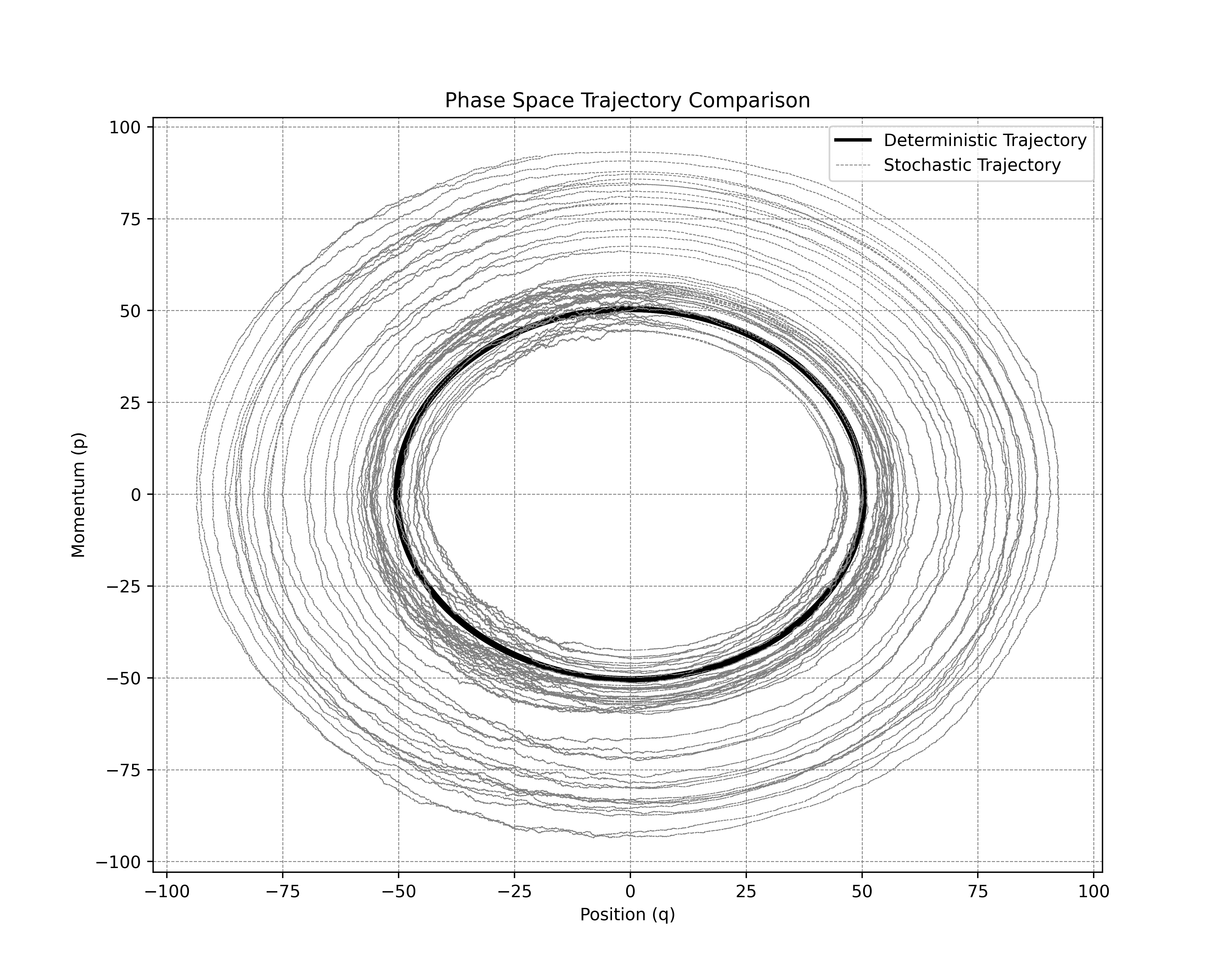
Figure 1. Comparison of phase space trajectories between the deterministic (bold solid line) and stochastically perturbed (thin dashed lines) harmonic oscillators. The system is modeled with the following parameters: mass $m=1$, spring constant $k=1$, time step $dt=0.0001$, and total simulation time $T=300$. The deterministic trajectory follows a stable circular orbit in phase space, indicating energy conservation and periodic motion. In contrast, the stochastic system introduces white noise perturbations using the Euler-Maruyama method, leading to diffusive and irregular trajectories that deviate from the original orbit over time.

When white noise perturbations are introduced, however, the trajectory deviates from this ideal path, displaying diffusion and irregularity. As shown in Fig.1, the stochastic oscillator’s trajectory gradually drifts away from the stable orbit, with random fluctuations disrupting the original pattern. This diffusion occurs because the noise introduces energy fluctuations, causing deviations in $p$ and $q$ that prevent strict adherence to the classical oscillator’s path. While some periodic behavior remains, the perturbations induce instability, leading to a trajectory that expands outward in phase space over time.

Nevertheless, we also observe that the stochastic oscillator’s phase space trajectories remain densely concentrated near the deterministic oscillator’s stable circular orbit. This aligns with our theoretical conclusions: the most probable path of the stochastically perturbed system stays close to the stable deterministic trajectory. This reinforces the understanding that, despite random perturbations, the system tends to evolve near the deterministic solution.

Fig.2 provides further insight by displaying the probability distribution of the Hamiltonian $H(q,p)$ for the stochastically perturbed oscillator. Notably, the Hamiltonian distribution $H_{S}$ peaks near $H_{S}=1249.6399$, closely matching the deterministic Hamiltonian value $H_{D}=1250$. This behavior supports our theoretical conclusion that the most probable Hamiltonian value for the stochastically perturbed system coincides with that of the deterministic system. For most of the time, the system’s Hamiltonian remains concentrated near the deterministic value, with large energy fluctuations being rare. This indicates that, despite random perturbations, the system’s overall evolution largely adheres to the conservation properties of the Hamiltonian system, with only local deviations due to noise.

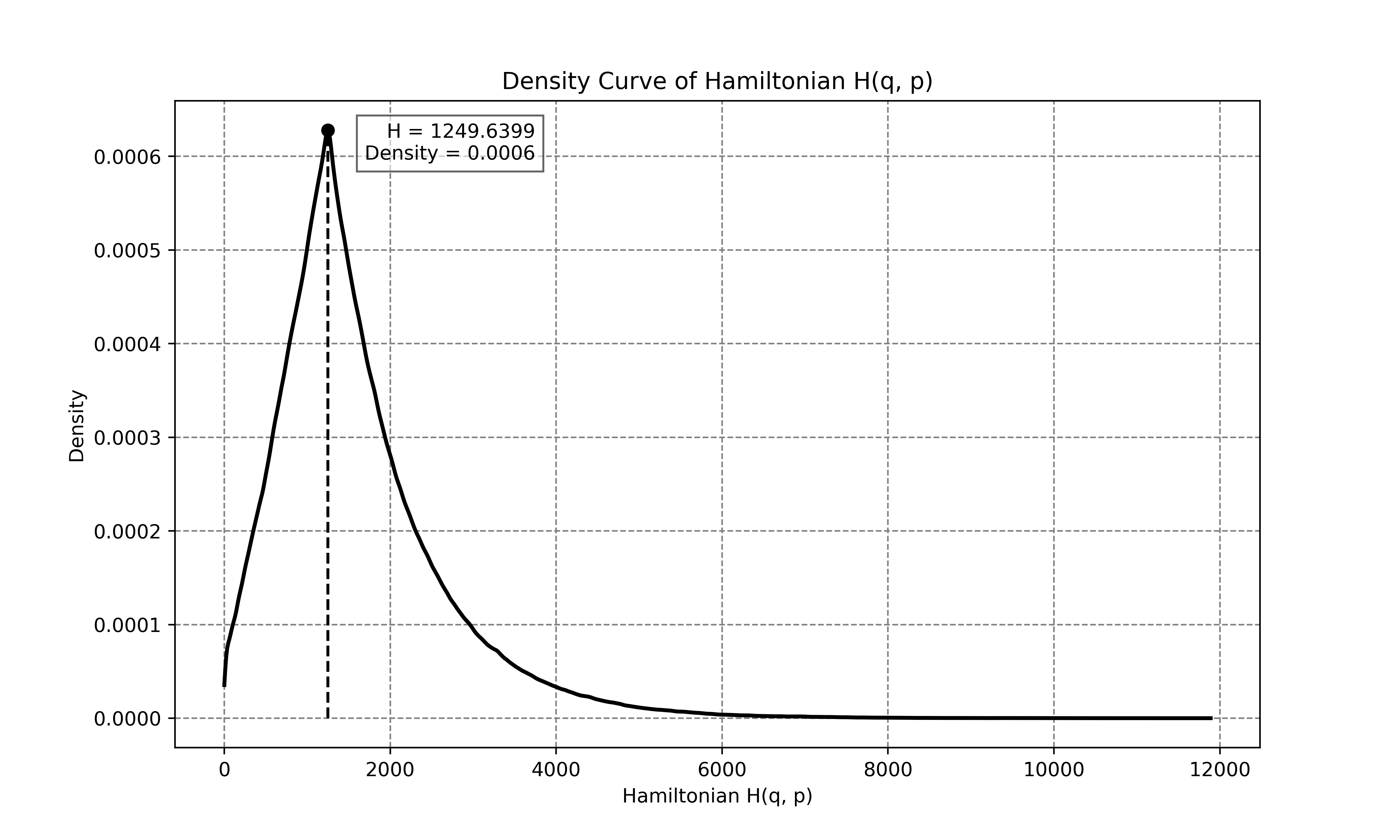
Figure 2. The distribution curve of the Hamiltonian $H(q,p)=\frac{p^{2}}{2m}+\frac{1}{2}kq^{2}$. The system is modeled with the following parameters: mass $m=1$, spring constant $k=1$, time step $dt=0.001$, total simulation time $T=300$, and 5000 simulation runs. The maximum value of the Hamiltonian $H$ is observed at 1249.6399, with a corresponding density of 0.0006. This result illustrates the distribution of the Hamiltonian in the presence of stochastic perturbations, showing that the system’s energy tends to concentrate around specific values in most cases.

In summary, Fig.1 and Fig.2 together illustrate the dynamics of both the classical Hamiltonian system and the stochastically perturbed system, revealing that the effects of random noise on the system’s trajectory and Hamiltonian are limited. Despite the introduction of stochastic perturbations, the system’s behavior remains closely aligned with that of the classical Hamiltonian system, supporting the theoretical conclusions derived from the Onsager-Machlup functional analysis. Next, we apply our results to a high-dimensional example.

Example 4.2.

Consider a simplified three-body system consisting of the Sun, Earth, and Moon. Given that the mass of the Sun ($m_{1}$) is significantly larger than those of the Earth ($m_{2}$) and Moon ($m_{3}$), we approximate the Sun as stationary, with the Earth and Moon moving within the Sun’s gravitational field. The specific parameters and Hamiltonian system are described below:
Sun:

• Mass: $m_{1}=1.989\times 10^{30}$.

• Position: $\vec{r}_{1}=(0,0,0)$.

Earth:

• Mass: $m_{2}=5.972\times 10^{24}$.

• Position: $\vec{r}_{2}=(x_{2},y_{2},z_{2})$.

• Initial Position at $t=0$: $(1.496\times 10^{11},0,0)$.

• Momentum: $\vec{p}_{2}=m_{2}\vec{\dot{r}}_{2}=(p_{x_{2}},p_{y_{2}},p_{z_{2}})$.

Moon:

• Mass: $m_{3}=7.348\times 10^{22}$.

• Position: $\vec{r}_{3}=(x_{3},y_{3},z_{3})$.

• Initial Position at $t=0$: $(1.496\times 10^{11}+3.844\times 10^{8},0,0)$.

• Momentum: $\vec{p}_{3}=m_{3}\vec{\dot{r}}_{3}=(p_{x_{3}},p_{y_{3}},p_{z_{3}})$.

The Gravitational Constant is given by $G=6.67430\times 10^{-11}$. The Kinetic Energy of the system can be expressed as:

$$T:=\frac{1}{2m_{2}}(p_{x_{2}}^{2}+p_{y_{2}}^{2}+p_{z_{2}}^{2})+\frac{1}{2m_{3}}(p_{x_{3}}^{2}+p_{y_{3}}^{2}+p_{z_{3}}^{2}).$$

Similarly, the Potential Energy is given by:

$$V:=-G\left(\frac{m_{1}m_{2}}{|\vec{r}_{2}|}+\frac{m_{1}m_{3}}{|\vec{r}_{3}|}+\frac{m_{2}m_{3}}{|\vec{r}_{3}-\vec{r}_{2}|}\right),$$

where the magnitudes of the position vectors are defined as:

$$|\vec{r}_{2}|=\sqrt{x_{2}^{2}+y_{2}^{2}+z_{2}^{2}},\quad|\vec{r}_{3}|=\sqrt{x_{3}^{2}+y_{3}^{2}+z_{3}^{2}},$$

$$|\vec{r}_{3}-\vec{r}_{2}|=\sqrt{(x_{3}-x_{2})^{2}+(y_{3}-y_{2})^{2}+(z_{3}-z_{2})^{2}}.$$

Therefore, the total energy $H$ of the system is:

$$H=\frac{1}{2m_{2}}(p_{x2}^{2}+p_{y2}^{2}+p_{z2}^{2})+\frac{1}{2m_{3}}(p_{x3}^{2}+p_{y3}^{2}+p_{z3}^{2})-G\left(\frac{m_{1}m_{2}}{|\vec{r}_{2}|}+\frac{m_{1}m_{3}}{|\vec{r}_{3}|}+\frac{m_{2}m_{3}}{|\vec{r}_{3}-\vec{r}_{2}|}\right).$$

In summary, the equations governing the motion of the Earth can be expressed as:

(4.4) $$\begin{cases}\dot{x}_{2}=\frac{p_{x_{2}}}{m_{2}},\\ \dot{p}_{x_{2}}=-Gm_{1}\frac{x_{2}}{|\vec{r}_{2}|^{3}}-Gm_{3}\frac{x_{2}-x_{3}}{|\vec{r}_{3}-\vec{r}_{2}|^{3}},\\ \dot{y}_{2}=\frac{p_{y_{2}}}{m_{2}},\\ \dot{p}_{y_{2}}=-Gm_{1}\frac{y_{2}}{|\vec{r}_{2}|^{3}}-Gm_{3}\frac{y_{2}-y_{3}}{|\vec{r}_{3}-\vec{r}_{2}|^{3}},\\ \dot{z}_{2}=\frac{p_{z_{2}}}{m_{2}},\\ \dot{p}_{z_{2}}=-Gm_{1}\frac{z_{2}}{|\vec{r}_{2}|^{3}}-Gm_{3}\frac{z_{2}-z_{3}}{|\vec{r}_{3}-\vec{r}_{2}|^{3}}.\end{cases}$$

Similarly, the equations governing the motion of the Moon can be expressed as:

(4.5) $$\begin{cases}\dot{x}_{3}=\frac{p_{x_{3}}}{m_{3}},\\ \dot{p}_{x_{3}}=-Gm_{1}\frac{x_{3}}{|\vec{r}_{3}|^{3}}-Gm_{2}\frac{x_{3}-x_{2}}{|\vec{r}_{3}-\vec{r}_{2}|^{3}},\\ \dot{y}_{3}=\frac{p_{y_{3}}}{m_{3}},\\ \dot{p}_{y_{3}}=-Gm_{1}\frac{y_{3}}{|\vec{r}_{3}|^{3}}-Gm_{2}\frac{y_{3}-y_{2}}{|\vec{r}_{3}-\vec{r}_{2}|^{3}},\\ \dot{z}_{3}=\frac{p_{z_{3}}}{m_{3}},\\ \dot{p}_{z_{3}}=-Gm_{1}\frac{z_{3}}{|\vec{r}_{3}|^{3}}-Gm_{2}\frac{z_{3}-z_{2}}{|\vec{r}_{3}-\vec{r}_{2}|^{3}}.\end{cases}$$

The normal three-body problem, when influenced by the perturbations from some other distant celestial bodies, can be abstractly modeled as the impact of random disturbances. We may define the three-body problem under random perturbations in the following form:
The Stochastic Equation for Earth’s Motion

(4.6) $$\begin{cases}{\rm d}x_{2}=\frac{p_{x_{2}}}{m_{2}}\,{\rm d}t+c_{21}(t)\,{\rm d}W_{21}(t),\\ {\rm d}p_{x_{2}}=-G\left(m_{1}\frac{x_{2}}{|\vec{r}_{2}|^{3}}+m_{3}\frac{x_{2}-x_{3}}{|\vec{r}_{3}-\vec{r}_{2}|^{3}}\right)\,{\rm d}t+c_{22}(t)\,{\rm d}W_{22}(t),\\ {\rm d}y_{2}=\frac{p_{y_{2}}}{m_{2}}\,{\rm d}t+c_{23}(t)\,{\rm d}W_{23}(t),\\ {\rm d}p_{y_{2}}=-G\left(m_{1}\frac{y_{2}}{|\vec{r}_{2}|^{3}}+m_{3}\frac{y_{2}-y_{3}}{|\vec{r}_{3}-\vec{r}_{2}|^{3}}\right)\,{\rm d}t+c_{24}(t)\,{\rm d}W_{24}(t),\\ {\rm d}z_{2}=\frac{p_{z_{2}}}{m_{2}}\,{\rm d}t+c_{25}(t)\,{\rm d}W_{25}(t),\\ {\rm d}p_{z_{2}}=-G\left(m_{1}\frac{z_{2}}{|\vec{r}_{2}|^{3}}+m_{3}\frac{z_{2}-z_{3}}{|\vec{r}_{3}-\vec{r}_{2}|^{3}}\right)\,{\rm d}t+c_{26}(t)\,{\rm d}W_{26}(t).\end{cases}$$

The Stochastic Equation for Moon’s Motion

(4.7) $$\begin{cases}{\rm d}x_{3}=\frac{p_{x_{3}}}{m_{3}}\,{\rm d}t+c_{31}(t)\,{\rm d}W_{31}(t),\\ {\rm d}p_{x_{3}}=-G\left(m_{1}\frac{x_{3}}{|\vec{r}_{3}|^{3}}+m_{2}\frac{x_{3}-x_{2}}{|\vec{r}_{3}-\vec{r}_{2}|^{3}}\right)\,{\rm d}t+c_{32}(t)\,{\rm d}W_{32}(t),\\ {\rm d}y_{3}=\frac{p_{y_{3}}}{m_{3}}\,{\rm d}t+c_{33}(t)\,{\rm d}W_{33}(t),\\ {\rm d}p_{y_{3}}=-G\left(m_{1}\frac{y_{3}}{|\vec{r}_{3}|^{3}}+m_{2}\frac{y_{3}-y_{2}}{|\vec{r}_{3}-\vec{r}_{2}|^{3}}\right)\,{\rm d}t+c_{34}(t)\,{\rm d}W_{34}(t),\\ {\rm d}z_{3}=\frac{p_{z_{3}}}{m_{3}}\,{\rm d}t+c_{35}(t)\,{\rm d}W_{35}(t),\\ {\rm d}p_{z_{3}}=-G\left(m_{1}\frac{z_{3}}{|\vec{r}_{3}|^{3}}+m_{2}\frac{z_{3}-z_{2}}{|\vec{r}_{3}-\vec{r}_{2}|^{3}}\right)\,{\rm d}t+c_{36}(t)\,{\rm d}W_{36}(t).\end{cases}$$

By substituting specific parameters, we compute the value of the Hamiltonian at the initial moment as $H_{0}\approx-2.706\times 10^{33}$. Furthermore, we obtain that the magnitudes of the positional derivatives $\dot{x}_{2}$, $\dot{y}_{2}$, and $\dot{z}_{2}$ for Earth are on the order of $10^{4}$, while the magnitudes of the momentum derivatives $\dot{p}_{x_{2}}$, $\dot{p}_{y_{2}}$, and $\dot{p}_{z_{2}}$ are on the order of $10^{22}$. For the Moon, the magnitudes of the positional derivatives $\dot{x}_{3}$, $\dot{y}_{3}$, and $\dot{z}_{3}$ are on the order of $10^{3}$, and those of the momentum derivatives $\dot{p}_{x_{3}}$, $\dot{p}_{y_{3}}$, and $\dot{p}_{z_{3}}$ are on the order of $10^{20}$.

From a physical perspective, the overall dynamical influence of external factors on the three-body system is relatively minor. Consequently, we set the intensity of random diffusion to be on the order of magnitude of $10^{-5}$ relative to its corresponding quantity. However, during the numerical simulation, to capture the long-time scale of the three-body problem (approximately $10^{18}$ seconds), we performed a time-scale transformation. Specifically, we shorten the time unit by a factor of $10^{16}$ (e.g., 1 second in the simulation now corresponds to $10^{16}$ seconds in reality). Thus, in the numerical simulation, $t\in[0,100]$ is equivalent to $t\in[0,10^{18}]$ in the real world. Since Brownian motion follows $W_{t}\;\sim\;\sqrt{t}$, the coefficient of the noise term needs to be scaled up by a factor of $10^{8}$. In summary, we define $c_{21}(t)=c_{23}(t)=c_{25}(t)=10^{7}$, $c_{22}(t)=c_{24}(t)=c_{26}(t)=10^{24}$, $c_{31}(t)=c_{33}(t)=c_{35}(t)=10^{6}$, and $c_{32}(t)=c_{34}(t)=c_{36}(t)=10^{23}$.

It is straightforward to verify that the aforementioned stochastic three-body equations satisfy Theorem 3.1. Utilizing Theorem $\eqref{T3.1}$ in conjunction with Euler-Lagrange equations, we deduce that the most probable path satisfies Equations $\eqref{4.4}$ and $\eqref{4.5}$. We numerically simulate the stochastic three-body problem equations $\eqref{4.6}$ and $\eqref{4.7}$ 10000 times, with each simulation spanning a time domain of $t\in[0,100]$ and a time step size set to 0.00001. For all simulations, we conduct statistical analysis on the Hamiltonian $H$ at 100 integer time points. The Fig.3 below depicts the density curve of the Hamiltonian $H$ obtained from our simulations.

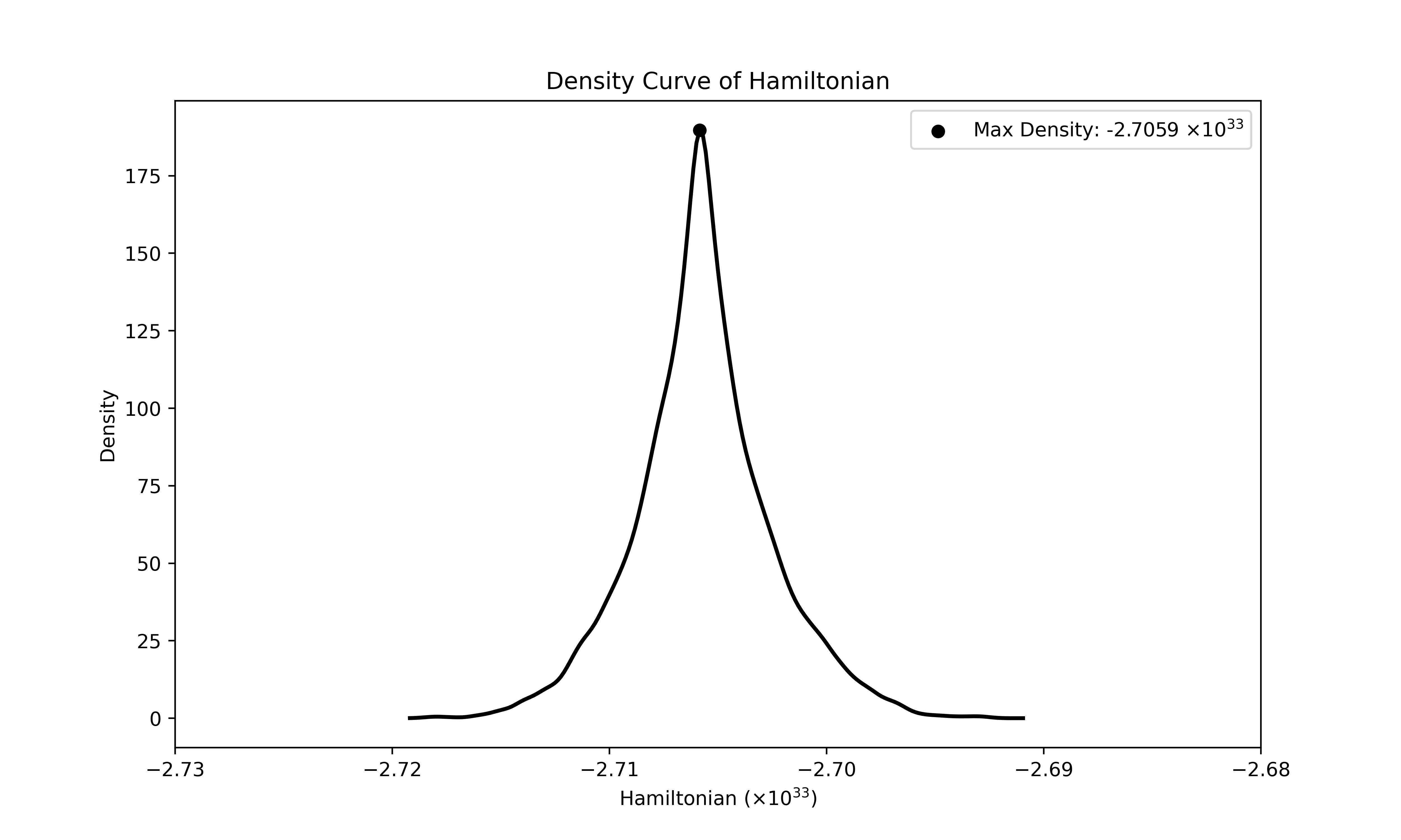
Figure 3. This represents the distribution curve of the Hamiltonian $H(q,p)$ for the three-body problem. Simulations indicate that the maximum value of the Hamiltonian $H$ is $-2.7059\times 10^{33}$. In the real physical world, the intensity of random perturbations is even smaller. Our numerical simulation results are consistent with the long-term evolution of a three-body system consisting of the Sun, Earth, and Moon, which maintains approximate energy conservation.

5. Large Deviation Principle and Rate Function for Stochastic Hamiltonian Systems

In this section, we derive the large deviation principle for stochastic Hamiltonian systems, combining the Onsager-Machlup functional and Freidlin-Wentzell theory [28]. Large deviation principle describes the probability behavior of a system’s trajectory deviating from the most probable path, with the rate function quantifying the decay rate of this probability.

Since our objective is to study the behavior of the trajectories in the stochastic Hamiltonian system as the noise term approaches zero, we simplify Equation (1.1) into the following form for convenience:

(5.1) $$\begin{cases}\mathrm{d}q(t)=\frac{\partial H}{\partial p}(q,p)\,\mathrm{d}t+\epsilon\sigma_{q}(t)\,\mathrm{d}W_{q}(t),\\ \mathrm{d}p(t)=-\frac{\partial H}{\partial q}(q,p)\,\mathrm{d}t+\epsilon\sigma_{p}(t)\,\mathrm{d}W_{p}(t),\end{cases}$$

where $q(t)$ and $p(t)$ represent the generalized position and momentum variables, respectively, and $H(q,p)$ is the Hamiltonian function describing the system’s energy, typically composed of kinetic and potential energy terms. $W_{q}(t)$ and $W_{p}(t)$ are independent Wiener processes, and the matrices $\sigma_{q}(t)$ and $\sigma_{p}(t)$ denote the diffusion coefficients for the stochastic components. The parameter $\epsilon$ represents the noise intensity. Our primary focus is on analyzing the statistical behavior of this system as $\epsilon\to 0$. Similar to Section 3, our result holds for any finite interval $t\in[0,T]$. For simplicity of notation, we will present the following theorem on the interval $[0,1]$.

Theorem 5.1.

Assuming that Conditions $C1$ and $C2$ hold, let $X^{\epsilon}:=(q(t),p(t))$ be the solution to the following stochastic Hamiltonian system (5.1). As $\epsilon\to 0$, the most probable path $\hat{\varphi}(t)=(\hat{\varphi}_{q}(t),\hat{\varphi}_{p}(t))$ is given by the deterministic Hamiltonian equations (4.1). For any path $X(t)=(q(t),p(t))$, the probability that the system deviates from the most probable path satisfies the large deviation principle:

(5.2) $$\epsilon^{2}\ln\mathbb{P}(X(t)\in A)\approx-\inf_{\varphi\in A}J(\varphi),$$

where $\varphi\in A$ denotes an arbitrarily continuous function, and $A\subset\mathbb{R}^{d}$ denote an arbitrary measurable set, and suppose that $\hat{\varphi}(t)\notin A$. Furthermore, the rate function $J(\varphi)$ is given by:

(5.3) $$J(\varphi)=\begin{cases}\frac{1}{2}\left(\int_{0}^{1}\left\|\sigma_{q}^{-1}(t)\left(\dot{\varphi}_{q}-\frac{\partial H}{\partial\varphi_{p}}(\varphi_{q},\varphi_{p})\right)\right\|^{2}\,{\rm d}t\right.\\ \left.+\int_{0}^{1}\left\|\sigma_{p}^{-1}(t)\left(\dot{\varphi}_{p}+\frac{\partial H}{\partial\varphi_{q}}(\varphi_{q},\varphi_{p})\right)\right\|^{2}\,{\rm d}t\right),&\text{if }\varphi-x_{0}\in\mathbb{H}^{1};\\ +\infty,&\text{otherwise}\end{cases}$$

with $\sigma_{q}^{-1}(t)$ and $\sigma_{p}^{-1}(t)$ being the inverses of the diffusion matrices $\sigma_{q}(t)$ and $\sigma_{p}(t)$, respectively.

Proof.

Equation $\eqref{17}$ merely concretizes the small random noise in Equation $\eqref{1}$ as being of order $\epsilon$, where $\epsilon$ is a small parameter. Therefore, we employ a definition and method similar to those used in the proof of Theorem 3.1. Let the reference path be given by $\varphi(t)=(\varphi_{q}(t),\varphi_{p}(t))$, where $\varphi(t)$ is a definite continuous path, and $(\varphi_{q}(t),\varphi_{p}(t))-(q(0),p(0))\in H^{1}$. We define the perturbed solution, denoted as $(y_{q}(t),y_{p}(t))$, as follows:

$$\begin{cases}y_{q}(t)=\varphi_{q}(t)+\epsilon\int_{0}^{t}\sigma_{q}(s)\,{\rm d}W_{q}(s),\\ y_{p}(t)=\varphi_{p}(t)+\epsilon\int_{0}^{t}\sigma_{p}(s)\,{\rm d}W_{p}(s).\end{cases}$$

To simplify the notation in the proof, we introduce the term $W^{\sigma}(t):=\left(W^{\sigma}_{q}(t),W^{\sigma}_{p}(t)\right)$, which encapsulates the stochastic perturbation in the system:

$$W^{\sigma}_{q}(t):=\int_{0}^{t}\sigma_{q}(s)\,{\rm d}W_{q}(s),\quad W^{\sigma}_{p}(t):=\int_{0}^{t}\sigma_{p}(s)\,{\rm d}W_{p}(s).$$

Then we introduce a new probability measure $\tilde{\mathbb{P}}$, under which the transformed Brownian motions are given by:

$$\tilde{W}_{q}(t) =W_{q}(t)-\frac{1}{\epsilon}\int_{0}^{t}\sigma_{q}^{-1}(s)\left(\frac{\partial H}{\partial y_{p}}(y_{q},y_{p})-\dot{\varphi}_{q}(s)\right)\,{\rm d}s,$$

$$\tilde{W}_{p}(t) =W_{p}(t)-\frac{1}{\epsilon}\int_{0}^{t}\sigma_{p}^{-1}(s)\left(-\frac{\partial H}{\partial y_{q}}(y_{q},y_{p})-\dot{\varphi}_{p}(s)\right)\,{\rm d}s.$$

Under this new measure $\tilde{\mathbb{P}}$, the system is purely driven by the new Brownian motions $\tilde{W}_{q}(t)$ and $\tilde{W}_{p}(t)$, free of the deterministic drift terms.

The Radon-Nikodym derivative $\mathcal{R}:=\frac{d\tilde{\mathbb{P}}}{d\mathbb{P}}$, representing the change of measure from $\mathbb{P}$ to $\tilde{\mathbb{P}}$, is given by the exponential martingale associated with the removed drift terms. For the position variable $q$, the Radon-Nikodym derivative is:

$$\frac{d\tilde{\mathbb{P}}_{q}}{d\mathbb{P}_{q}}=\exp \left\{\frac{1}{\epsilon}\int_{0}^{1}\left\langle\sigma_{q}^{-1}(s)\left(\frac{\partial H}{\partial y_{p}}(y_{q},y_{p})-\dot{\varphi}_{q}(s)\right),\,{\rm d}W_{q}(s)\right\rangle\right.$$

$$\left.-\frac{1}{2\epsilon^{2}}\int_{0}^{1}\left|\sigma_{q}^{-1}(s)\left(\frac{\partial H}{\partial y_{p}}(y_{q},y_{p})-\dot{\varphi}_{q}(s)\right)\right|^{2}\,{\rm d}s\right\},$$

and similarly for the momentum variable $p$:

$$\frac{d\tilde{\mathbb{P}}_{p}}{d\mathbb{P}_{p}}=\exp \left\{\frac{1}{\epsilon}\int_{0}^{1}\left\langle\sigma_{p}^{-1}(s)\left(-\frac{\partial H}{\partial y_{q}}(y_{q},y_{p})-\dot{\varphi}_{p}(s)\right),\,{\rm d}W_{p}(s)\right\rangle\right.$$

$$\left.-\frac{1}{2\epsilon^{2}}\int_{0}^{1}\left|\sigma_{p}^{-1}(s)\left(\frac{\partial H}{\partial y_{q}}(y_{q},y_{p})+\dot{\varphi}_{p}(s)\right)\right|^{2}\,{\rm d}s\right\}.$$

Thus,

$$\mathcal{R}=\exp \left\{\frac{1}{\epsilon}\left(\int_{0}^{1}\left\langle\sigma_{q}^{-1}(s)\left(\frac{\partial H}{\partial y_{p}}(y_{q},y_{p})-\dot{\varphi}_{q}(s)\right),\,{\rm d}W_{q}(s)\right\rangle\right.\right.$$

$$\qquad\left.-\int_{0}^{1}\left\langle\sigma_{p}^{-1}(s)\left(\frac{\partial H}{\partial y_{q}}(y_{q},y_{p})+\dot{\varphi}_{p}(s)\right),\,{\rm d}W_{p}(s)\right\rangle\right)$$

$$-\frac{1}{2\epsilon^{2}}\left(\int_{0}^{1}\left|\sigma_{q}^{-1}(s)\left(\frac{\partial H}{\partial y_{p}}(y_{q},y_{p})-\dot{\varphi}_{q}(s)\right)\right|^{2}\,{\rm d}s\right.$$

$$\qquad\left.\left.+\int_{0}^{1}\left|\sigma_{p}^{-1}(s)\left(\frac{\partial H}{\partial y_{q}}(y_{q},y_{p})+\dot{\varphi}_{p}(s)\right)\right|^{2}\,{\rm d}s\right)\right\}.$$

Define

$$K(\varphi,\epsilon)=\{x-x_{0}\in\mathbb{H}^{1}\mid\varphi-x_{0}\in\mathbb{H}^{1},\|x-\varphi\|\leq\epsilon,\epsilon>0\}.$$

Utilizing Girsanov’s Theorem, we aim to compute the probability that the trajectory of the solution $X(t)$ of the stochastic Hamiltonian system remains in close proximity to a reference path $\varphi(t)$ when the noise intensity $\epsilon$ is minimal. Then

(5.4) $$\quad\mathbb{P}(X(t)\in K(\varphi,\epsilon))=\mathbb{P}\left(\left\|(q,p)-(\varphi_{q},\varphi_{p})\right\|\leq\epsilon\right)$$

$$=\tilde{\mathbb{P}}\left(\left\|(Y_{q},Y_{p})-(\varphi_{q},\varphi_{p})\right\|\leq\delta\right)=\mathbb{E}\left(\mathcal{R}\mathbb{I}_{\left\|W^{\sigma}\right\|\leq 1}\right)$$

$$=\mathbb{E}\left(\mathcal{R}\big{|}{\left\|W^{\sigma}\right\|\leq 1}\right)\times\mathbb{P}(\left\|W^{\sigma}\right\|\leq 1)$$

$$=\exp\left\{-\frac{1}{2\epsilon^{2}}\left(\int_{0}^{1}\left\|\sigma_{q}^{-1}(t)\left(\dot{\varphi}_{q}-\frac{\partial H}{\partial\varphi_{p}}(\varphi_{q},\varphi_{p})\right)\right\|^{2}\,{\rm d}t\right.\right.$$

$$\qquad\qquad\qquad\qquad\left.\left.+\int_{0}^{1}\left\|\sigma_{p}^{-1}(t)\left(\dot{\varphi}_{p}+\frac{\partial H}{\partial\varphi_{q}}(\varphi_{q},\varphi_{p})\right)\right\|^{2}\,{\rm d}t\right)\right\}$$

$$\quad\times\mathbb{E}\left(\exp\left\{\frac{1}{\epsilon^{2}}\sum_{i=1}^{6}B_{i}\right\}\mathbb{I}_{\left\|W^{\sigma}\right\|\leq 1}\right)\times\mathbb{P}(\left\|W^{\sigma}\right\|\leq 1),$$

where $B_{i}$ represents the deviations in the path arising from drift and disturbances, it exhibits stochastic properties. This is elaborated upon in the following detailed expressions:

$$B_{1} =\epsilon\int_{0}^{1}\left\langle\sigma_{q}^{-1}(s)\frac{\partial H}{\partial y_{p}}(y_{q},y_{p}),\,{\rm d}W_{q}(s)\right\rangle-\epsilon\int_{0}^{1}\left\langle\sigma_{p}^{-1}(s)\frac{\partial H}{\partial y_{q}}(y_{q},y_{p}),\,{\rm d}W_{p}(s)\right\rangle,$$

$$B_{2} =-\epsilon\int_{0}^{1}\left\langle\sigma_{q}^{-1}(s)\dot{\varphi}_{q}(s),\,{\rm d}W_{q}(s)\right\rangle-\epsilon\int_{0}^{1}\left\langle\sigma_{p}^{-1}(s)\dot{\varphi}_{p}(s),\,{\rm d}W_{p}(s)\right\rangle,$$

$$B_{3} =\frac{1}{2}\int_{0}^{1}\left\|\sigma_{q}^{-1}(s)\frac{\partial H}{\partial\varphi_{p}}(\varphi_{q},\varphi_{p})\right\|^{2}\,{\rm d}s-\frac{1}{2}\int_{0}^{1}\left\|\sigma_{q}^{-1}(s)\frac{\partial H}{\partial y_{p}}(y_{q},y_{p})\right\|^{2}\,{\rm d}s,$$

$$B_{4} =\frac{1}{2}\int_{0}^{1}\left\|\sigma_{p}^{-1}(s)\frac{\partial H}{\partial\varphi_{q}}(\varphi_{q},\varphi_{p})\right\|^{2}\,{\rm d}s-\frac{1}{2}\int_{0}^{1}\left\|\sigma_{p}^{-1}(s)\frac{\partial H}{\partial y_{q}}(y_{q},y_{p})\right\|^{2}\,{\rm d}s,$$

$$B_{5} =\int_{0}^{1}\left\langle\sigma_{q}^{-2}(s)\left(\frac{\partial H}{\partial y_{p}}(y_{q},y_{p})-\frac{\partial H}{\partial\varphi_{p}}(\varphi_{q},\varphi_{p})\right),\dot{\varphi}_{q}(s)\right\rangle\,{\rm d}s,$$

$$B_{6} =-\int_{0}^{1}\left\langle\sigma_{p}^{-2}(s)\left(\frac{\partial H}{\partial y_{q}}(y_{q},y_{p})-\frac{\partial H}{\partial\varphi_{q}}(\varphi_{q},\varphi_{p})\right),\dot{\varphi}_{p}(s)\right\rangle\,{\rm d}s.$$

We decompose the system’s probability into a deterministic part

$$\exp \left\{-\frac{1}{2\epsilon^{2}}\left(\int_{0}^{1}\left\|\sigma_{q}^{-1}(t)\left(\dot{\varphi}_{q}-\frac{\partial H}{\partial\varphi_{p}}(\varphi_{q},\varphi_{p})\right)\right\|^{2}\,{\rm d}t\right.\right.$$

$$\qquad\quad\left.\left.+\int_{0}^{1}\left\|\sigma_{p}^{-1}(t)\left(\dot{\varphi}_{p}+\frac{\partial H}{\partial\varphi_{q}}(\varphi_{q},\varphi_{p})\right)\right\|^{2}\,{\rm d}t\right)\right\}$$

a correction part

$$\mathbb{E}\left(\exp\left\{\frac{1}{\epsilon^{2}}\sum_{i=1}^{6}B_{i}\big{|}{\left\|W^{\sigma}\right\|\leq 1}\right\}\right),$$

and small ball probabilities for Brownian motion

$$\mathbb{P}(\left\|W^{\sigma}\right\|\leq 1).$$

Specifically, the deterministic component represents the behavior along the deterministic trajectory, while the correction component accounts for deviations induced by random perturbations. The small ball probabilities for Brownian motion represent fixed values that are intrinsically linked to the diffusion coefficients $\sigma_{q}$, $\sigma_{p}$, and the duration of time, yet they are independent of the variable $\varphi$. Furthermore, for convenience, we introduce the notation $U(\varphi)$ defined as:

$$U(\varphi):=\left\|\sigma_{q}^{-1}(t)\left(\dot{\varphi}_{q}-\frac{\partial H}{\partial\varphi_{p}}(\varphi_{q},\varphi_{p})\right)\right\|^{2}+\left\|\sigma_{p}^{-1}(t)\left(\dot{\varphi}_{p}+\frac{\partial H}{\partial\varphi_{q}}(\varphi_{q},\varphi_{p})\right)\right\|^{2}.$$

Large deviation theory focuses on large-scale deviations, and in this context, we are particularly concerned with the $\frac{1}{\epsilon^{2}}$ scale. Given the boundedness of $\sigma_{q,i}^{-1}(s)$ and $\sigma_{p,i}^{-1}(s)$, along with the fact that $H\in C^{3}_{b}(\mathbb{R}^{n}\times\mathbb{R}^{n},\mathbb{R})$, we can infer that

(5.5) $$\limsup\limits_{\epsilon\to 0}\mathbb{E}\left({\rm exp}\left\{cB_{1}\right\}\big{|}{\left\|W^{\sigma}\right\|\leq 1}\right)=1,$$

and

(5.6) $$\limsup\limits_{\epsilon\to 0}\mathbb{E}\left({\rm exp}\left\{cB_{2}\right\}\big{|}{\left\|W^{\sigma}\right\|\leq 1}\right)=1.$$

For the third term $B_{3}$,

$$B_{3} =\frac{1}{2}\int_{0}^{1}\left\|\sigma_{q}^{-1}(s)\frac{\partial H}{\partial\varphi_{p}}(\varphi_{q},\varphi_{p})\right\|^{2}\,{\rm d}s-\frac{1}{2}\int_{0}^{1}\left\|\sigma_{q}^{-1}(s)\frac{\partial H}{\partial y_{p}}(y_{q},y_{p})\right\|^{2}\,{\rm d}s$$

$$\leq\frac{1}{2}\int_{0}^{1}{\sigma_{q}^{-2}(s)\left\|\frac{\partial H}{\partial\varphi_{p}}(\varphi_{q},\varphi_{p})-\frac{\partial H}{\partial y_{p}}(y_{q},y_{p})\right\|^{2}}$$

$$\quad+{2\sigma_{q}^{-2}(s)\left\|\frac{\partial H}{\partial\varphi_{p}}(\varphi_{q},\varphi_{p})-\frac{\partial H}{\partial y_{p}}(y_{q},y_{p})\right\|\left\|\frac{\partial H}{\partial y_{p}}(y_{q},y_{p})\right\|}\,{\rm d}s$$

$$\leq\frac{1}{2}\int_{0}^{1}{\sigma_{q}^{-2}(s)\left\|\frac{\partial H}{\partial\varphi_{p}}(\varphi_{q},\varphi_{p})-\frac{\partial H}{\partial y_{p}}(y_{q},y_{p})\right\|^{2}}\,{\rm d}s$$

$$\quad+\int_{0}^{1}{\sigma_{q}^{-2}(s)\left\|\frac{\partial H}{\partial\varphi_{p}}(\varphi_{q},\varphi_{p})-\frac{\partial H}{\partial y_{p}}(y_{q},y_{p})\right\|\left\|\frac{\partial H}{\partial y_{p}}(y_{q},y_{p})\right\|}\,{\rm d}s.$$

Using that $\frac{\partial H}{\partial p}$ is Lipschitz continuous, we have

(5.7) $$\quad\left\|\frac{\partial H}{\partial y_{p}}(y_{q},y_{p})-\frac{\partial H}{\partial\varphi_{p}}(\varphi_{q},\varphi_{p})\right\|$$

$$=\left\|\frac{\partial H}{\partial\left(\varphi_{p}+\epsilon W^{\sigma}_{p}\right)}((\varphi_{q}+\epsilon W^{\sigma}_{q}),(\varphi_{p}+\epsilon W^{\sigma}_{p}))-\frac{\partial H}{\partial\varphi_{p}}(\varphi_{q},\varphi_{p})\right\|$$

$$\leq L\epsilon\left\|W^{\sigma}\right\|.$$

Inequality $\eqref{5.7}$ and the boundedness of $\frac{\partial H}{\partial y_{p}}(y_{q},y_{p})$ and $\sigma_{q}^{-1}(t)$ imply that

(5.8) $$\limsup\limits_{\epsilon\to 0}\mathbb{E}\left({\rm exp}\left\{cB_{3}\right\}\big{|}{\left\|W^{\sigma}\right\|\leq 1}\right)=1$$

for all $c\in\mathbb{R}$.

For the fourth term $B_{4}$, employing the same proof technique as for the third term $B_{3}$, we have

(5.9) $$\limsup\limits_{\epsilon\to 0}\mathbb{E}\left({\rm exp}\left\{cB_{4}\right\}\big{|}{\left\|W^{\sigma}\right\|\leq 1}\right)=1$$

for all $c\in\mathbb{R}$.

For the fifth term $B_{5}$, applying inequality $\eqref{5.7}$ and the boundedness of $\dot{\varphi}_{q}(t)$ and $\sigma_{q}^{-1}(t)$, we have

$$B_{5} =\int_{0}^{1}\left\langle\sigma_{q}^{-2}(s)\left(\frac{\partial H}{\partial y_{p}}(y_{q},y_{p})-\frac{\partial H}{\partial\varphi_{p}}(\varphi_{q},\varphi_{p})\right),\dot{\varphi}_{q}(s)\right\rangle\,{\rm d}s$$

$$\leq C\left\|\frac{\partial H}{\partial y_{p}}(y_{q},y_{p})-\frac{\partial H}{\partial\varphi_{p}}(\varphi_{q},\varphi_{p})\right\|$$

$$\leq CL\epsilon\left\|W^{\sigma}\right\|.$$

Thus,

(5.10) $$\limsup\limits_{\epsilon\to 0}\mathbb{E}\left({\rm exp}\left\{cB_{5}\right\}\big{|}{\left\|W^{\sigma}\right\|\leq 1}\right)=1$$

for all $c\in\mathbb{R}$.

For the sixth term $B_{6}$, employing the same proof technique as for the fifth term $B_{5}$, we have

(5.11) $$\limsup\limits_{\epsilon\to 0}\mathbb{E}\left({\rm exp}\left\{cB_{6}\right\}\big{|}{\left\|W^{\sigma}\right\|\leq 1}\right)=1$$

for all $c\in\mathbb{R}$.

Based on the outcomes derived from Equations $\eqref{5.4}$-$\eqref{5.6}$ and $\eqref{5.8}$-$\eqref{5.11}$, we can ascertain the explicit form of the rate function by utilizing both the upper and lower bounds of the probability estimate. Here, we solely focus on the scenario where $\varphi-x_{0}\in\mathbb{H}^{1}$, and for the remaining scenarios, we directly assign $J=\infty$.

On one hand, we estimate the upper bound of this probability. Suppose that $F$ is a closed set, and under the guarantee of the continuity of the function $U$, we can envision the existence of a sequence of compact sets $\{K_{n}\}$ satisfying $K_{n}\subset F$ and such that $\inf_{\varphi\in K_{n}}U(\varphi)$ converges to $\inf_{\varphi\in F}U(\varphi)$.

For each compact set $K_{n}$ and any $\epsilon>0$, there always exist a finite number of continuous curves $\{\varphi_{j}\}_{j=1}^{N}\subset K_{n}$ and their corresponding neighborhoods $K(\varphi_{j},\epsilon)$ such that:

$$K_{n}\subset\bigcup_{j=1}^{N}K(\varphi_{j},\epsilon).$$

Applying the union bound principle to this finite covering, we obtain:

$$\mathbb{P}((X(t)\in K_{n})\leq\sum_{j=1}^{N}\mathbb{P}((X(t)\in K(\varphi_{j},\epsilon)).$$

Taking the logarithm of the above inequality and multiplying by $\epsilon^{2}$, we get:

$$\epsilon^{2}\ln\mathbb{P}((X(t)\in K_{n}) \leq\epsilon^{2}\ln\left(N\cdot\max_{1\leq j\leq N}\mathbb{P}((X(t)\in K(\varphi_{j},\epsilon))\right)$$

$$\leq\epsilon^{2}\ln N+\max_{1\leq j\leq N}\epsilon^{2}\ln\mathbb{P}((X(t)\in K(\varphi_{j},\epsilon)).$$

Taking the upper limit $\limsup\limits_{\epsilon\to 0}$ of the above equation, we obtain:

$$\limsup_{\epsilon\to 0}\epsilon^{2}\ln\mathbb{P}((X(t)\in K_{n})\leq\max_{1\leq j\leq N}\left(\limsup_{\epsilon\to 0}\epsilon^{2}\ln\mathbb{P}((X(t)\in K(\varphi_{j},\epsilon))\right).$$

Since $\epsilon^{2}\ln N$ tends to 0, the dominant term is determined by the neighborhood with the maximum probability. Combining the above proofs, we have:

$$\limsup_{\epsilon\to 0}\epsilon^{2}\ln\mathbb{P}((X(t)\in K_{n}) \leq\lim_{\epsilon\to 0}\max_{1\leq j\leq N}\left(-\frac{1}{2}\int_{0}^{1}U(\varphi_{j})\,{\rm d}s\right.$$

$$\quad\left.+\mathbb{E}\left(\sum_{i=1}^{6}B_{i}\mid\left\|W^{\sigma}\right\|\leq 1\right)+\epsilon^{2}\ln\mathbb{P}(\left\|W^{\sigma}\right\|\leq 1)\right)$$

$$\leq\max_{1\leq j\leq N}\left(-\frac{1}{2}\int_{0}^{1}U(\varphi_{j})\,{\rm d}s\right)$$

$$\leq-\min_{1\leq j\leq N}\frac{1}{2}\int_{0}^{1}U(\varphi_{j})\,{\rm d}s.$$

Since $\{\varphi_{j}\}\subset K_{n}$, we get:

$$\min_{1\leq j\leq N}\int_{0}^{1}U(\varphi_{j})\,{\rm d}s\geq\inf_{\varphi\in K_{n}}\int_{0}^{1}U(\varphi_{j})\,{\rm d}s.$$

Therefore

$$\limsup_{\epsilon\to 0}\epsilon^{2}\ln\mathbb{P}((X(t)\in K_{n})\leq-\inf_{\varphi\in K_{n}}\frac{1}{2}\int_{0}^{1}U(\varphi_{j})\,{\rm d}s.$$

For any $\delta>0$, there exists a compact set $K_{n}\subset F$ such that:

$$\inf_{\varphi\in F}\int_{0}^{1}U(\varphi_{j})\,{\rm d}s+\delta\geq\inf_{\varphi\in K_{n}}\int_{0}^{1}U(\varphi_{j})\,{\rm d}s\geq\inf_{\varphi\in F}\int_{0}^{1}U(\varphi_{j})\,{\rm d}s-\delta.$$

Since $\mathbb{P}((X(t)\in F)\leq\mathbb{P}((X(t)\in K_{n})+\mathbb{P}((X(t)\in F\setminus K_{n})$, and the probability of the part outside the compact set decays exponentially to 0 as $n$ increases, the main contribution comes from $K_{n}$. Therefore, as $n$ tends to infinity and $\epsilon$ tends to 0, we obtain:

(5.12) $$\limsup_{\epsilon\to 0}\epsilon^{2}\ln\mathbb{P}((X(t)\in F)\leq-\inf_{\varphi\in F}\frac{1}{2}\int_{0}^{1}U(\varphi_{j})\,{\rm d}s.$$

On the other hand, we estimate the lower bound of this probability. Let $G$ be an arbitrary open set in $\mathbb{R}^{n}$. For any $\varphi\in G$, it holds that

$$\lim_{{\epsilon\to 0}}\mathbb{P}((X(t)\in G)\geq\lim_{{\epsilon\to 0}}\mathbb{P}(X^{\epsilon}\in K(\varphi,\epsilon)).$$

Since $\varphi\in G$ is arbitrarily chosen, we have

$$\lim_{{\epsilon\to 0}}\mathbb{P}((X(t)\in G)\geq\lim_{\epsilon\to 0}\sup_{\varphi\in G}\mathbb{P}(X^{\epsilon}\in K(\varphi,\epsilon)).$$

That is,

(5.13) $$\liminf_{{\epsilon\to 0}}\epsilon^{2}\ln\mathbb{P}(X(t)\in G)\geq-\inf_{\varphi\in G}\frac{1}{2}\int_{0}^{1}U(\varphi)\,{\rm d}s.$$

By combining the upper bound inequality (5.12) and the lower bound inequality (5.13), we can derive the rate function for the stochastic Hamiltonian system:

$$J(\varphi) =\frac{1}{2}\left(\int_{0}^{1}\left\|\sigma_{q}^{-1}(t)\left(\dot{\varphi}_{q}-\frac{\partial H}{\partial\varphi_{p}}(\varphi_{q},\varphi_{p})\right)\right\|^{2}\,{\rm d}t\right.$$

$$\qquad\left.+\int_{0}^{1}\left\|\sigma_{p}^{-1}(t)\left(\dot{\varphi}_{p}+\frac{\partial H}{\partial\varphi_{q}}(\varphi_{q},\varphi_{p})\right)\right\|^{2}\,{\rm d}t\right).$$

∎

6. Preservation of Invariant Tori in Nearly Integrable Stochastic Hamiltonian Systems

In this section, we investigate the Onsager-Machlup functional, most probable paths, and large deviation principles in nearly integrable Hamiltonian systems with stochastic perturbations. By integrating these findings with KAM theory, we further examine the persistence of invariant tori in almost integrable Hamiltonian systems under small stochastic perturbations, particularly in the most probable sense. To apply KAM theory, in classical mechanics, converting generalized coordinates and momenta into action-angle variables greatly simplifies the analysis of integrable systems.

Firstly, we introduce some notations that will be used throughout this section:

• The $d$-dimensional torus is denoted by $\mathbb{T}^{d}:=\mathbb{R}^{d}/2\pi\mathbb{Z}^{d}$.

• For $\alpha>0$ and $\tau\geq d-1\geq 1$, the set of $(\alpha,\tau)$-Diophantine numbers in $\mathbb{R}^{d}$ is defined as

  $$\Delta_{\alpha}^{\tau}:=\left\{\omega\in\mathbb{R}^{d}:|\omega\cdot k|\geq\frac{\alpha}{|k|_{1}^{\tau}},\forall 0\neq k\in\mathbb{Z}^{d}\right\}.$$

• The Lebesgue (outer) measure on $\mathbb{R}^{d}$ is denoted by $meas$.

• For $l\in\mathbb{R}$, the integer part is denoted by $[l]$ and the fractional part by $\{l\}$.

• For $l>0$ and an open subset $A$ of $\mathbb{R}^{d}$ or $\mathbb{R}^{d}\times\mathbb{T}^{d}$, the set $C^{l}(A)$ consists of continuously differentiable functions $f$ on $A$ up to the order $[l]$ such that $f^{[l]}$ is Hölder-continuous with exponent $\{l\}$ and with finite $C^{l}$-norm defined by:

  $$\|f\|_{C^{l}(A)} :=\max\left\{\|f\|_{C^{[l]}(A)},\|f^{[l]}\|_{C^{\{l\}}(A)}\right\},$$

  $$\|f\|_{C^{[l]}(A)} :=\max_{\begin{subarray}{c}k\in\mathbb{N}^{d}\\ 0\leq|k|_{1}\leq[l]\end{subarray}}\sup_{A}|\partial_{I}^{k}f|,$$

  $$\|f^{[l]}\|_{C^{\{l\}}(A)} :=\max_{\begin{subarray}{c}k\in\mathbb{N}^{d}\\ |k|_{1}=[l]\end{subarray}}\sup_{\begin{subarray}{c}I_{1},I_{2}\in A\\ 0<|I_{1}-I_{2}|<1\end{subarray}}\frac{|\partial_{I}^{k}f(I_{1})-\partial_{I}^{k}f(I_{2})|}{|I_{1}-I_{2}|^{\{l\}}}.$$

  When $A=\mathbb{R}^{d}$ or $A=\mathbb{R}^{d}\times\mathbb{T}^{d}$, we simplify this to $\|f\|_{C^{l}}$.

• For $l>0$ and any subset $A$ of $\mathbb{R}^{d}$, $C_{W}^{l}(A)$ denotes the set of functions of class $C^{l}$ on $A$ in the sense of Whitney.

• For $r,s>0$, $y_{0}\in\mathbb{C}^{d}$, and $\varnothing\neq\mathscr{D}\subseteq\mathbb{C}^{d}$, we define:

  $$\begin{split}\mathbb{T}_{s}^{d}&:=\left\{x\in\mathbb{C}^{d}:|\text{Im }x|<s\right\}/2\pi\mathbb{Z}^{d},\\ B_{r}(y_{0})&:=\left\{y\in\mathbb{R}^{d}:|y-y_{0}|<r\right\},\quad(y_{0}\in\mathbb{R}^{d}),\\ D_{r}(y_{0})&:=\left\{y\in\mathbb{C}^{d}:|y-y_{0}|<r\right\},\\ D_{r,s}(y_{0})&:=D_{r}(y_{0})\times\mathbb{T}_{s}^{d},\\ D_{r,s}(\mathscr{D})&:=\bigcup_{y_{0}\in\mathscr{D}}D_{r,s}(y_{0}).\end{split}$$

• The unit $(d\times d)$ matrix is denoted by $\mathbb{I}_{d}:=\text{diag}(1)$, and the standard symplectic matrix is given by

  $$\mathbb{J}:=\begin{pmatrix}0&-\mathbb{I}_{d}\\ \mathbb{I}_{d}&0\end{pmatrix}.$$

• For $\mathscr{D}\subseteq\mathbb{C}^{d}$, $A_{r,s}(\mathscr{D})$ denotes the Banach space of real-analytic functions with bounded holomorphic extensions to $D_{r,s}(\mathscr{D})$, with norm

  $$\|\cdot\|_{r,s,\mathscr{D}}:=\sup_{D_{r,s}(\mathscr{D})}|\cdot|.$$

• The canonical symplectic form on $\mathbb{C}^{d}\times\mathbb{C}^{d}$ is given by

  $$\omega:=d\theta\land dI=d\theta_{1}\land dI_{1}+\cdots+d\theta_{d}\land dI_{d},$$

  and $\phi_{H}^{t}$ denotes the associated Hamiltonian flow governed by the Hamiltonian $H(I,\theta)$, $I,\theta\in\mathbb{C}^{d}$.

• The projections on the first and last $d$-components are denoted by $\pi_{1}:\mathbb{C}^{d}\times\mathbb{C}^{d}\ni(I,\theta)\longmapsto I$ and $\pi_{2}:\mathbb{C}^{d}\times\mathbb{C}^{d}\ni(I,\theta)\longmapsto\theta$, respectively.

• For a linear operator $\mathcal{L}$ from the normed space $(V_{1},\|\cdot\|_{1})$ into the normed space $(V_{2},\|\cdot\|_{2})$, its ”operator norm” is given by

  $$\|\mathcal{L}\|:=\sup_{x\in V_{1}\setminus\{0\}}\frac{\|\mathcal{L}x\|_{2}}{\|x\|_{1}},$$

  so that $\|\mathcal{L}x\|_{2}\leq\|\mathcal{L}\|\|x\|_{1}$ for any $x\in V_{1}$.

• For $\omega\in\mathbb{R}^{d}$ and a $C^{1}$ function $f$, the directional derivative of $f$ with respect to $\omega$ is given by

  $$D_{\omega}f:=\omega\cdot f_{I}=\sum_{j=1}^{d}\omega_{j}f_{I_{j}}.$$

• If $f$ is a smooth or analytic function on $\mathbb{T}^{d}$, its Fourier expansion is given by

  $$f=\sum_{k\in\mathbb{Z}^{d}}f_{k}e^{ik\cdot\theta},\quad f_{k}:=\frac{1}{(2\pi)^{d}}\int_{\mathbb{T}^{d}}f(\theta)e^{-ik\cdot\theta}d\theta,$$

  where $e:=\exp(1)$ denotes the Neper number and $i$ the imaginary unit. We also set:

  $$\langle f\rangle:=f_{0}=\frac{1}{(2\pi)^{d}}\int_{\mathbb{T}^{d}}f(\theta)d\theta.$$

Without loss of generality, the Hamiltonian equations for an integrable system are expressed as:

(6.1) $$\begin{cases}d\theta(t)=\frac{\partial H}{\partial I}(I(t))\,dt=\omega(I(t))\,dt,\\ dI(t)=0,\end{cases}$$

where $I$ are action variables, $\theta$ are angle variables, and $\omega(I)$ are frequencies associated with the action variables. For an integrable system, the action variables $I$ remain constant over time, while the angle variables $\theta$ evolve linearly with time.

When introducing a small deterministic perturbation $\epsilon_{1}P(I,\theta)$, the almost integrable Hamiltonian becomes:

$$H_{\epsilon}(I,\theta)=H(I)+\epsilon_{1}P(I,\theta),$$

and the corresponding Hamiltonian equations in action-angle variables take the following form:

(6.2) $$\begin{cases}\mathrm{d}\theta(t)=\frac{\partial H_{\epsilon}}{\partial I}(I(t),\theta(t))\,\mathrm{d}t,\\ \mathrm{d}I(t)=-\frac{\partial H_{\epsilon}}{\partial\theta}(I(t),\theta(t))\,\mathrm{d}t.\end{cases}$$

In this scenario, the action variables $I$ are no longer constant and undergo slight changes due to the perturbation, while the evolution of the angle variables $\theta$ is correspondingly modified.

When a small stochastic perturbation $\epsilon_{2}\sigma(t)\,dW(t)$ is further introduced, the corresponding stochastic Hamiltonian system in action-angle variables is described by the following stochastic differential equations:

(6.3) $$\begin{cases}\mathrm{d}\theta(t)=\frac{\partial H_{\epsilon}}{\partial I}(I(t),\theta(t))\,\mathrm{d}t+\epsilon_{2}\sigma_{\theta}(t)\,\mathrm{d}W_{\theta}(t),\\ \mathrm{d}I(t)=-\frac{\partial H_{\epsilon}}{\partial\theta}(I(t),\theta(t))\,\mathrm{d}t+\epsilon_{2}\sigma_{I}(t)\,\mathrm{d}W_{I}(t),\end{cases}$$

where $\epsilon_{2}$ represents the strength of the stochastic perturbation, $\sigma_{\theta}(t)$ and $\sigma_{I}(t)$ are the diffusion coefficients, and $W_{\theta}(t)$ and $W_{I}(t)$ are independent Wiener processes.

We then investigate the invariant tori associated with the Hamiltonian

$$H_{\epsilon}(I,\theta)=H(I)+\epsilon_{1}P(I,\theta),$$

corresponding to Equation (6.2). The following assumptions are imposed:

1. Let $l>2\nu:=2(\tau+1)>2d\geq 4$, and let $\mathscr{D}\subset\mathbb{R}^{d}$ be a non - empty, bounded domain.

2. Consider the Hamiltonian $H_{\epsilon}(I,\theta)$ on the phase space $\mathscr{D}\times\mathbb{T}^{d}$. Here, $H$ and $P$ are given functions in $C^{l}(\mathscr{D}\times\mathbb{T}^{d})$ with finite $l$ - norms $\|H\|_{C^{l}(\mathscr{D})}$ and $\|P\|_{C^{l}(\mathscr{D})}$.

3. Assume that $H_{I}$ is locally uniformly invertible. This implies that for all $I\in\mathscr{D}$, $\det H_{II}(I)\neq 0$. To simplify notation, define $T(I):=H_{II}(I)^{-1}$, and suppose that $C_{T}:=\|T\|_{C^{0}(\mathscr{D})}<\infty$. Furthermore, set $C_{H}:=\max\left\{1,\|H\|_{C^{l}(\mathscr{D})}\right\}$, and then define $\theta:=C_{T}C_{H}$, which possesses the property that $\theta\geq 1$.

4. Let $\alpha\in(0,1)$ and set,

   $$\quad\alpha_{*}:=\alpha^{\frac{1}{l-2v}},\quad\mathscr{D}^{\prime}:=\{I\in\mathscr{D}:B_{\alpha_{*}}(I)\subseteq\mathscr{D}\},\quad\mathscr{D}_{\alpha}:=\{I\in\mathscr{D}^{\prime}:H_{I}(I)\in\Delta^{\tau}_{\alpha}\}.$$

5. Finally, for some suitable constant $C_{1}=C_{1}(d,l)>1$, set

   $$\begin{cases}\sigma:=\left(\frac{\varepsilon^{3/2}}{\theta^{2l/\nu}\alpha\sqrt{C_{H}}}\right)^{1/(l+\nu)},\\ \rho:=\frac{2C_{1}C_{H}\varepsilon}{\alpha^{2}\sigma^{2\nu}},\\ \beta_{0}:=\min\left\{\frac{l}{2\nu}-1+\frac{1}{\nu},2\right\}.\end{cases}$$

Under the aforementioned notation and assumptions (C1), (C2), and (H1)-(H5), the following stochastic version of the KAM theorem holds.

Theorem 6.1.

Consider the stochastic Hamiltonian system given by $\eqref{6.3}$, where the diffusion coefficients $\sigma_{\theta}(t)$ and $\sigma_{I}(t)$ satisfy condition (C2), and the Hamiltonian $H_{\epsilon}(I,\theta)$ is sufficiently smooth and satisfies condition (C1). Then, the Onsager-Machlup functional for system $\eqref{6.3}$ is given by:

$$OM(\varphi_{\theta},\varphi_{I}) =\frac{1}{\epsilon_{2}^{2}}\left(\int_{0}^{1}\left\|\sigma_{\theta}^{-1}(t)\left(\dot{\varphi_{\theta}}-\omega(\varphi_{I})-\epsilon_{1}\frac{\partial P}{\partial\varphi_{I}}(\varphi_{\theta},\varphi_{I})\right)\right\|^{2}\,{\rm d}t\right.$$

$$\qquad\left.+\int_{0}^{1}\left\|\sigma_{I}^{-1}(t)\left(\dot{\varphi_{I}}+\epsilon_{1}\frac{\partial P}{\partial\varphi_{\theta}}(\varphi_{\theta},\varphi_{I})\right)\right\|^{2}\,{\rm d}t\right).$$

Furthermore, by applying the variational principle to minimize the Onsager-Machlup functional, the most probable transition path can be obtained, corresponding to the solution of the nearly integrable Hamiltonian system Equation $\eqref{6.2}$.

Additionally, when conditions (H1)-(H5) hold, the invariant tori of the original integrable system Equation (6.1) remain preserved under both deterministic and stochastic perturbations, albeit with slight deformation, in the sense of most probable. Let $X_{\epsilon}(t)$ represent the solution of system $\eqref{6.3}$, and $\mathcal{K}$ denote the collection of invariant tori in the nearly integrable Hamiltonian system $\eqref{6.2}$. According to the large deviation principle provided by Theorem $\eqref{T5.1}$, we have:

$$\epsilon_{2}^{2}\ln\mathbb{P}(X_{\epsilon}(t)\in A)\approx-\inf_{\varphi\in A}I(\varphi),$$

where $A\in\mathbb{R}^{d}$ denotes an arbitrary measurable set and the rate function $I(\varphi)$ is given by:

$$I(\varphi) =\frac{1}{2}\left(\int_{0}^{1}\left\|\sigma_{\theta}^{-1}(t)\left(\dot{\varphi_{\theta}}-\omega(\varphi_{I})-\epsilon_{1}\frac{\partial P}{\partial\varphi_{I}}(\varphi_{\theta},\varphi_{I})\right)\right\|^{2}\,{\rm d}t\right.$$

$$\qquad\left.+\int_{0}^{1}\left\|\sigma_{I}^{-1}(t)\left(\dot{\varphi_{I}}+\epsilon_{1}\frac{\partial P}{\partial\varphi_{\theta}}(\varphi_{\theta},\varphi_{I})\right)\right\|^{2}\,{\rm d}t\right).$$

Proof.

Under Conditions (C1) and (C2), the Onsager-Machlup functional for system $\eqref{6.3}$ can be directly obtained through Theorem 3.1. By minimizing this Onsager-Machlup functional, we find that the most probable continuous path of the nearly integrable stochastic Hamiltonian system coincides with the solution of the deterministic nearly integrable Hamiltonian equation $\eqref{6.2}$. For a more precise statement, please refer to Sections 3 and 4.

Next, we will outline the framework for proving the existence of invariant tori and the measure of Cantor sets, with detailed proofs referred to in [26]. This commences by extending $H$ and $P$ to the entirety of the phase space $\mathbb{R}^{d}\times\mathbb{T}^{d}$. To accomplish this extension, we introduce a cut-off function $\chi\in C(\mathbb{C}^{d})\cap C^{\infty}(\mathbb{R}^{d})$ that fulfills the conditions $0\leq\chi\leq 1$, with its support confined within $D_{\alpha_{*}}(\mathscr{D}^{\prime})$ and $\chi$ being identically equal to 1 on $D_{\alpha_{*}/2}(\mathscr{D}^{\prime})$. Additionally, for any multi-index $k\in\mathbb{N}^{d}$ with $|k|_{1}\leq l$, there exists a constant $C_{0}=C_{0}(d,l)>0$ such that

$$\|\partial_{y}^{k}\chi\|_{\mathbb{R}^{d}}\leq C_{0}\alpha_{*}^{-|k|_{1}}.$$

Utilizing Faà Di Bruno’s Formula [7], we construct $\widehat{H}\in C^{l}(\mathbb{R}^{d})$ such that $\|T\|_{\mathscr{D}}\|\widehat{H}-H\|_{C^{l}(\mathscr{D})}\leq C_{1}^{-1}\alpha_{*}^{l}/4$. Consequently, $\widehat{H}_{II}=H_{II}(\mathbb{I}_{d}+T(\widehat{H}_{II}-H_{II}))$ is invertible on $\mathscr{D}$ with $\|(\widehat{H}_{II})^{-1}\|_{\mathscr{D}}\leq 2\|T\|_{\mathscr{D}}$.

Defining $\tilde{H}:=\widehat{H}+\chi\cdot(H-\widehat{H})$, we ensure $\tilde{H}\in C^{l}(\mathbb{R}^{d}\times\mathbb{T}^{d})$ and $\tilde{H}\equiv H$ on $D_{\alpha_{*}/2}(\mathscr{D}^{\prime})$. Furthermore,

$$\|\tilde{H}\|_{C^{l}}\leq\|H\|_{C^{l}}+C_{1}\alpha_{*}^{-l}\|\widehat{H}-H\|_{C^{l}}<2\|H\|_{C^{l}},$$

and

$$\|(\widehat{H}_{II})^{-1}\partial_{y}^{2}(\chi\cdot(H-\widehat{H}))\|_{\mathscr{D}}\leq\|(\widehat{H}_{II})^{-1}\|_{\mathscr{D}}\cdot C_{1}\alpha_{*}^{-l}\|\widehat{H}-H\|_{C^{l}}\leq 1/2.$$

Thus, $\tilde{H}_{II}$ is invertible with $\|(\tilde{H}_{II})^{-1}\|_{\mathscr{D}}\leq 2\|(\widehat{H}_{II})^{-1}\|_{\mathscr{D}}\leq 4\|T\|_{\mathscr{D}}$.

Similarly, $P$ is extended to a function $\tilde{P}\in C^{l}(\mathbb{R}^{d}\times\mathbb{T}^{d})$ such that $\tilde{P}\equiv P$ on $D_{\alpha_{*}/2}(\mathscr{D}^{\prime})$ and $\|P\|_{C^{l}}\leq 2\|P\|_{C^{l}}$. Setting $\tilde{H}_{\epsilon}:=\tilde{H}+\tilde{P}$, we observe $\tilde{H}_{\epsilon}|_{D_{\alpha_{*}/2}(\mathscr{D}^{\prime})}={H}_{\epsilon}$. Notably, replacing ${H}_{\epsilon}$ with $\tilde{H}_{\epsilon}$ makes no difference since the invariant tori of $\tilde{H}_{\epsilon}$ we aim to construct reside within $D_{\alpha_{*}/2}(\mathscr{D}^{\prime})$, given $r_{0}<\alpha_{*}/2$.

Let $\mathcal{D}\subset\mathbb{R}^{d}$ be a domain with a smooth boundary $\partial\mathcal{D}$. Suppose there exists a positive constant $c=c(d,\tau,l)<1$ such that the parameters $\alpha$ and $\varepsilon$ satisfy the following conditions:

$$0<\alpha\leq\min\left\{cC_{H},\frac{R(\mathcal{D})}{6},\frac{1}{2}\,\mathrm{minfoc}(\partial\mathcal{D})\right\},\quad\varepsilon\leq cC_{H}^{-\frac{l+2v}{l-2v}}\theta^{-a}\alpha^{\frac{2l}{l-2v}},$$

where $R(\mathcal{D}):=\sup\{R>0:B_{R}(I)\subseteq\mathcal{D}\text{ for some }I\in\mathcal{D}\}$, $\mathrm{minfoc}(\partial\mathcal{D})$ is the minimal focal distance of $\partial\mathcal{D}$ and $a:=(l-2v)^{-1}\max\left\{(6+2lv^{-1})(l+v)-2l(l-v),\right.$ $\left.2l(l+3v)v^{-1}\right\}$.

Let $\mathcal{H}_{j}$ (resp. $\mathcal{P}_{j}$) denote the real-analytic approximation $H_{\xi_{j}}$ (resp. $P_{\xi_{j}}$) of $\tilde{H}$ (resp. $\tilde{P}$) defined on $\mathcal{O}_{j}$, as given by Lemma 2.15. Define the initial set $\mathscr{D}_{0}$ as:

$$\mathscr{D}_{0}:=\{I\in\mathbb{R}^{d}:\partial_{I}\mathcal{H}_{0}(I)\in\partial_{I}H(\mathscr{D}_{\alpha})\}.$$

For $j\geq 1$, we define the proposition $(\mathscr{P}_{j})$ as follows: There exist:

1. A sequence of sets $\mathscr{D}_{j}$,

2. A sequence of diffeomorphisms $G_{j}:D_{\tilde{r}_{j}}(\mathscr{D}_{j-1})\to G_{j}(D_{\tilde{r}_{j}}(\mathscr{D}_{j-1}))$,

3. A sequence of real-analytic symplectic transformations

   $$\Phi_{j}=(v_{j},u_{j}):D_{r_{j},s_{j}}(\mathscr{D}_{j})\to D_{\sigma_{j-1},\sigma_{j-1}}(\mathscr{D}_{j-1}),$$

such that, setting $\mathcal{H}^{\epsilon}_{j-1}:=\mathcal{H}_{j-1}+\mathcal{P}_{j-1}$, the following properties hold:

$$G_{j}(\mathscr{D}_{j-1})=\mathscr{D}_{j}\subset\mathscr{D}_{r_{j}},\quad G_{j}=(\partial_{I}H_{j})^{-1}\circ\partial_{I}H_{j-1},$$

$$\det\partial_{I}^{2}H_{j}(y)\neq 0,\quad T_{j}(I):=\partial_{I}^{2}H_{j}(I)^{-1},\quad\forall I\in\mathscr{D}_{j},$$

$$H^{\epsilon}_{j}:=\mathcal{H}^{\epsilon}_{j-1}\circ\phi^{j}:=H_{j}+P_{j}\quad\text{on }D_{r_{j},s_{j}}(\mathscr{D}_{j}),$$

where $\phi^{j}:=\phi_{1}\circ\phi_{2}\circ\cdots\circ\phi_{j}$ and $K_{0}:=\mathcal{K}_{0}$.

Moreover,

$$\left\lVert G_{j}-\text{id}\right\rVert_{\tilde{r}_{j},\mathscr{D}_{j-1}}\leq\tilde{r}_{j}\xi^{2\nu}\xi^{m(j-1)},\quad\left\lVert\partial_{y}G_{j}-\mathbb{I}_{d}\right\rVert_{\tilde{r}_{j},\mathscr{D}_{j-1}}\leq\xi^{2\nu}\xi^{2m(j-1)},$$

$$\left\lVert\partial_{I}^{2}H_{j}\right\rVert_{r_{j},\mathscr{D}_{j}}<2C_{H},\quad\left\lVert T_{j}\right\rVert_{\mathscr{D}_{j}}<2C_{T},\quad T_{j}:=(\partial_{I}^{2}H_{j})^{-1},\quad\left\lVert P_{j}\right\rVert_{r_{j},s_{j},\mathscr{D}_{j}}\leq C_{1}C_{H}\xi_{j}^{l-1},$$

$$\max\left\{\left\lVert M_{j}(\phi_{j}-\text{id})\right\rVert_{2r_{j},s_{j},\mathscr{D}_{j}},\left\lVert\pi_{2}\partial_{x}(\phi_{j}-\text{id})\right\rVert_{2r_{j},s_{j},\mathscr{D}_{j}}\right\}\leq\xi^{2\nu}\xi^{m(j-1)},$$

where $M_{j}:=\text{diag}(r_{j}^{-1}\mathbb{I}_{d},\sigma_{j}^{-1}\mathbb{I}_{d})$.

We will use mathematical induction to prove that the proposition $(\mathscr{P}_{j})$ holds for all $j\geq 1$. The proof of this part primarily relies on the application of Lemma 2.14. It is straightforward to verify that Lemma 2.14 can be applied to $\mathcal{H}^{\epsilon}_{0}$, which implies that the statement $(\mathscr{P}_{1})$ holds.

Next, we assume that $(\mathscr{P}_{j})$ holds for some $j\geq 1$ and proceed to prove $(\mathscr{P}_{j+1})$. First, observe the following estimates:

$$s_{j}+\frac{\sigma_{j-1}}{3}=\frac{(12\xi+1)\sigma_{j-1}}{3}<\frac{2\sigma_{j-1}}{3}<\frac{s_{j-1}}{2},$$

$$2r_{j}+\frac{r_{j-1}\sigma_{j-1}}{3}<\frac{r_{j-1}}{4}+\frac{r_{j-1}}{6}<\frac{r_{j-1}}{2},$$

$$2r_{j}+\frac{r_{j-1}\sigma_{j-1}}{3}<\sigma_{0}^{\nu}\xi^{j}+\frac{\sigma_{j-1}}{3}=\sigma_{0}^{\tau}\sigma_{j}+\frac{\sigma_{j-1}}{3}<\sigma_{j-1}.$$

These inequalities, combined with a symplectic change of coordinates $\phi^{\prime}=\text{id}+\tilde{\phi}:D_{\overline{r}/2,s^{\prime}}(\mathscr{D}^{\prime})\to D_{\overline{r}+r\sigma/3,\overline{s}}(\mathscr{D})$ in Lemma 2.14, imply that

(6.4) $$\phi_{j}(D_{r_{j},s_{j}}(\mathscr{D}_{j}))\subset D_{\sigma_{j-1},\sigma_{j-1}}(\mathscr{D}_{j-1})\bigcap D_{r_{j-1}/2,s_{j-1}/2}(\mathscr{D}_{j-1}).$$

In particular, the real-analytic symplectic transformation

$$\phi_{j}=(v_{j},u_{j}):D_{r_{j},s_{j}}(\mathscr{D}_{j})\to D_{\sigma_{j-1},\sigma_{j-1}}(\mathscr{D}_{j-1}),$$

exists. Furthermore, the inequality

$$2r_{j+1}<\frac{1}{4}\min\left\{\frac{\alpha}{2d(2C_{H})\kappa_{j}^{\nu}},\check{r}_{j+1}\right\}$$

holds. Together with the definitions of the sequences of the various parameters, this ensures that condition (2.2) in Lemma 2.14 is satisfied for all $j\geq 1$.

Write

$$\mathcal{H}^{\epsilon}_{j}:=\mathcal{H}_{j}+\mathcal{P}_{j}=\mathcal{H}^{\epsilon}_{j-1}+(\mathcal{H}_{j}-\mathcal{H}_{j-1})+(\mathcal{P}_{j}-\mathcal{P}_{j-1})$$

By the inductive assumption and (6.4), we have

$$\mathcal{H}^{\epsilon}_{j}\circ\phi^{j} =\mathcal{H}^{\epsilon}_{j-1}\circ\phi^{j}+(\mathcal{H}_{j}-\mathcal{H}_{j-1})\circ v^{j}+(\mathcal{P}_{j}-\mathcal{P}_{j-1})\circ\phi^{j}$$

$$=H_{j}+P_{j}+(\mathcal{H}_{j}-\mathcal{H}_{j-1})\circ v_{j}+(\mathcal{P}_{j}-\mathcal{P}_{j-1})\circ\phi^{j}$$

$$=\mathcal{H}^{j}+\mathcal{P}^{j},\quad\text{on }D_{r_{j},s_{j}}(\mathscr{D}_{j}),$$

where $\mathcal{H}^{j}:=H_{j}$ and $\mathcal{P}^{j}:=P_{j}+(\mathcal{H}_{j}-\mathcal{H}_{j-1})\circ\phi^{j}+(\mathcal{P}_{j}-\mathcal{P}_{j-1})\circ\phi^{j}$, with

(6.5) $$\left\lVert\partial_{y}^{2}\mathcal{H}^{j}\right\rVert_{r_{j},\mathscr{D}_{j}}<2C_{K},\qquad\left\lVert(\partial_{y}^{2}\mathcal{H}^{j})^{-1}\right\rVert_{\mathscr{D}_{j}}<2C_{T},$$

by the inductive assumption, provided $\phi^{j}$ maps $D_{r_{j},s_{j}}(\mathscr{D}_{j})$ into $\mathcal{O}_{j}=\{(I,\theta)\in\mathbb{C}^{d}\times\mathbb{C}^{d}:|\text{Im}(I,\theta)|<\xi_{j}\}$ i.e.

(6.6) $$\sup_{D_{r_{j},s_{j}}(\mathscr{D}_{j})}|\text{Im}\phi^{j}|\leq\frac{\xi_{j}}{2}.$$

Hence,

$$\left\lVert\mathcal{P}^{j}\right\rVert_{r_{j},s_{j},\mathscr{D}_{j}} \leq\left\lVert P_{j}\right\rVert_{r_{j},s_{j},\mathscr{D}_{j}}+\left\lVert(\mathcal{H}_{j}-\mathcal{H}_{j-1})\circ\phi^{j}\right\rVert_{r_{j},s_{j},\mathscr{D}_{j}}+\left\lVert(\mathcal{P}_{j}-\mathcal{P}_{j-1})\circ\phi^{j}\right\rVert_{r_{j},s_{j},\mathscr{D}_{j}}$$

$$\leq C_{1}C_{H}\xi_{j-1}^{l}+\left\lVert\mathcal{H}_{j}-\mathcal{H}_{j-1}\right\rVert_{\xi_{j}}+\left\lVert\mathcal{P}_{j}-\mathcal{P}_{j-1}\right\rVert_{\xi_{j}}$$

$$\leq C_{1}C_{H}\xi_{j-1}^{l}+C_{1}C_{H}\xi_{j-1}^{l}+C_{1}\varepsilon\xi_{j-1}^{l}$$

$$\leq 3C_{1}C_{H}\xi_{j-1}^{l}.$$

Thus, thanks to (6.5), $\mathcal{H}^{\epsilon}_{j}\circ\phi^{j}=\mathcal{H}^{j}+\mathcal{P}^{j}$ satisfies the assumptions in (2.1) with $\varepsilon\sim\left\lVert\mathcal{P}^{j}\right\rVert_{r_{j},s_{j},\mathscr{D}_{j}}$, $r\sim r_{j}$, $s\sim s_{j}$, $\sigma\sim\sigma_{j}$, $C_{H}\sim 2C_{H}$ as

$$\partial_{I}^{2}\mathcal{H}^{j}(\mathscr{D}_{j})\stackrel{{\scriptstyle\text{def}}}{{=}}\partial_{I}^{2}H_{j}(G_{j}(\mathscr{D}_{j-1}))=\partial_{I}^{2}H_{j-1}(\mathscr{D}_{j-1})=\cdots=\partial_{I}^{2}H_{0}(\mathscr{D}_{0})\subset\Delta_{\tau}^{\alpha}.$$

Hence, in order to apply Lemma 6 to $\mathcal{H}^{\epsilon}_{j}\circ\phi^{j}=\mathcal{H}^{j}+\mathcal{P}^{j}$, we only need to check (2.3). Upon observation, we have

$$r_{j}=r_{0}\xi^{\nu j}\leq\frac{\alpha}{2C_{H}}\sigma_{j}^{\nu}\leq\alpha\sigma_{j}^{\nu}/\left\lVert\partial_{I}^{2}\mathcal{H}^{j}\right\rVert_{r_{j},s_{j},\mathscr{D}_{j}},$$

$$\sigma_{1}^{-\nu}\frac{\left\lVert\mathcal{P}^{1}\right\rVert_{r_{1},s_{1},\mathscr{D}_{1}}}{\alpha r_{1}}\rho^{-1}\leq C_{2}\sigma_{0}^{l}\frac{C_{H}}{\varepsilon\xi^{2\nu}}\leq 1,$$

$$3C_{0}\frac{\theta C_{T}\left\lVert\mathcal{P}^{1}\right\rVert_{r_{1},s_{1},\mathscr{D}_{1}}}{r_{1}\check{r}_{2}\bar{\sigma}_{1}}\leq C_{2}\sigma_{0}^{l-2\nu}\frac{\theta^{6+m}(C_{H})^{2}}{\alpha^{2}}\lambda^{2(\nu+m)}\leq\xi^{2\nu},$$

and, for $j\geq 2$,

$$\sigma_{j}^{-\nu}\frac{\left\lVert\mathcal{P}^{j}\right\rVert_{r_{j},s_{j},\mathscr{D}_{j}}}{\alpha r_{j}}\rho^{-1}\leq C_{2}\sigma_{0}^{l}\frac{C_{H}}{\varepsilon}\xi^{(l-2\nu)j-2l}\leq C_{2}\sigma_{0}^{l}\frac{C_{H}}{\varepsilon}\xi^{-2l}\leq 1,$$

$$3C_{0}\frac{\theta C_{T}\left\lVert\mathcal{P}^{j}\right\rVert_{r_{j},s_{j},\mathscr{D}_{j}}}{r_{j}\check{r}_{j+1}\bar{\sigma}_{j}}\leq C_{2}\sigma_{0}^{l-2\nu}\frac{\theta^{4+2l/\nu}(C_{H})^{2}}{\alpha^{2}}\lambda^{2l}\leq\xi^{2\nu}.$$

Therefore, Lemma 6 applies to $\mathcal{H}^{\epsilon}_{j}$ and yields the desired symplectic change of coordinates $\phi_{j+1}$.

Furthermore, based on Lemmas 2.15 and 2.16, we can obtain the convergence results for $G^{j}$, $P_{j}$, $\phi^{j}$, and $H_{j}$ as follows:

• The sequence $G^{j}:=G_{j}\circ G_{j-1}\circ\cdots\circ G_{2}\circ G_{1}$ converges uniformly on $\mathscr{D}_{0}$ to a diffeomorphism $G_{*}:\mathscr{D}_{0}\to\mathscr{D}_{*}:=G_{*}(\mathscr{D}_{0})\subset\mathscr{D}$, and $G_{*}\in C_{W}^{1}(\mathscr{D}_{0})$.

• $P_{j}$ converges uniformly to 0 on $\mathscr{D}_{*}\times\mathbb{T}_{s_{*}}^{d}$ in the $C_{W}^{2}$ topology.

• $\phi^{j}$ converges uniformly on $\mathscr{D}_{*}\times\mathbb{T}^{d}$ to a symplectic transformation

  $$\phi_{*}:\mathscr{D}_{*}\times\mathbb{T}^{d}\stackrel{{\scriptstyle\text{into}}}{{\longrightarrow}}\mathscr{D}\times\mathbb{T}^{d},$$

  with $\phi_{*}\in C_{W}^{\tilde{m}}(\mathscr{D}_{*}\times\mathbb{T}^{d})$ and $\phi_{*}(\cdot,\cdot)\in C^{\tilde{m}v}(\mathbb{T}^{d})$, for any given $y_{*}\in\mathscr{D}_{*}$.

• $H_{j}$ converges uniformly on $\mathscr{D}_{*}$ to a function $H_{*}\in C_{W}^{2+\tilde{m}}(\mathscr{D}_{*})$, with

  $$\partial_{I_{*}}H_{*}\circ G_{*}=\partial_{I}\mathcal{H}_{0},\qquad\qquad\qquad\text{on }\mathscr{D}_{0},$$

  $$H\circ\phi_{*}(I_{*},x)=H_{*}(I_{*}),\qquad\forall(I_{*},x)\in\mathscr{D}_{*}\times\mathbb{T}^{d}.$$

Based on the preceding proof, we can demonstrate that there exists a Cantor-like set $\mathcal{D}_{*}\subset\mathcal{D}$, an embedding $\phi_{*}=(v_{*},u_{*}):\mathcal{D}_{*}\times\mathbb{T}^{d}\rightarrow\mathcal{H}:=\phi_{*}(\mathcal{D}_{*}\times\mathbb{T}^{d})\subset\mathcal{D}\times\mathbb{T}^{d}$ of class $C_{W}^{\beta}(\mathcal{D}_{*}\times\mathbb{T}^{d})$, and a function $H_{*}\in C_{W}^{2}(\mathcal{D}_{*},\mathbb{R})$, such that $H^{\epsilon}\circ\phi_{*}(I_{*},\theta)=K_{*}(I_{*},\theta)$ for all $(I_{*},\theta)\in\mathcal{D}_{*}\times\mathbb{T}^{d}$. The map $\xi\mapsto\phi_{*}(I_{*},\theta)$ is of class $C_{\beta}^{v}(\mathbb{T}^{d})$ for any $I_{*}\in\mathcal{D}_{*}$ (with $v^{-1}<\beta<\beta_{0}$), and the map $G^{*}:=(\partial_{I_{*}}H_{*})^{-1}\circ\partial_{I}H:\mathcal{D}_{*}\rightarrow\mathcal{D}_{*}$ defines a lipeomorphism onto $\mathcal{D}_{*}$, satisfying $B_{\alpha/2}(\mathcal{D}_{*})\subseteq\mathcal{D}$. The set $\mathcal{K}$ is foliated by KAM tori of $H^{\epsilon}$, each being a graph of a $C^{v}(\mathbb{T}^{d})$-map.

Furthermore, the following estimates hold:

$$\|G^{*}-\mathrm{id}\|_{\mathcal{D}_{*}}\leq\varepsilon^{\frac{3\tau}{2(l+v)}}\alpha^{\frac{l+1}{l+v}}C_{H}^{\frac{\tau}{2(l+v)}}\theta^{-1}L^{\frac{2l\tau}{v(l+v)}},\quad\|G^{*}-\mathrm{id}\|_{L,\mathcal{D}_{*}}<\frac{1}{2},$$

and

$$\sup_{\mathcal{D}_{*}\times\mathbb{T}^{d}}\max\left\{|M(\phi_{*}-\mathrm{id})|,\,\|\pi_{2}(\partial_{x}\phi_{*}-\mathbb{I}_{d})\|\right\}\leq 8\theta^{-2}(\log\rho^{-1})^{-2v}<1,$$

where $M:=\mathrm{diag}\left(C_{H}(\alpha\sigma^{v})^{-1}\mathbb{I}_{d},\sigma^{-1}\mathbb{I}_{d}\right)$.

Then, the measure of the complement of $\mathcal{K}$ is bounded by

$$\mathrm{meas}(\mathcal{D}\times\mathbb{T}^{d}\setminus\mathcal{K})\leq(3\pi)^{d}\left(2\mathcal{H}^{d-1}(\partial\mathcal{D})\tilde{\epsilon}+C\tilde{\epsilon}^{2}+\mathrm{meas}(\mathcal{D}^{\prime}\setminus\mathcal{D}_{\alpha})\right),$$

with

$$\tilde{\epsilon}:=\max\left\{\epsilon^{\frac{3\tau}{2(l+v)}}\alpha^{\frac{l+1}{l+v}}C_{H}^{\frac{-\tau}{2(l+v)}}\theta^{-1}L^{\frac{2l\tau}{v(l+v)}},\alpha_{*}\right\},C=2\sum_{j=1}^{\left\lfloor\frac{d-1}{2}\right\rfloor}\frac{\tilde{\epsilon}^{2j-1}{k}_{2j}(\mathbb{R}^{\partial\mathcal{D}})}{1\cdot 3\cdots(2j+1)},$$

where ${k}_{2j}(\mathbb{R}^{\partial\mathcal{D}})$ denotes the $(2j)$-th integrated mean curvature of $\partial\mathcal{D}$.

Finally, from Theorem 5.1, we derive the large deviation principle for the nearly integrable stochastic Hamiltonian system: as $\epsilon\to 0$, the most probable path $\hat{\varphi}(t)=(\hat{\varphi}_{\theta}(t),\hat{\varphi}_{I}(t))$ is given by the deterministic nearly integrable Hamiltonian equation $\eqref{6.2}$. For any path $X_{\epsilon}(t)=(\theta(t),I(t))$ of equation $\eqref{6.3}$, the probability of deviating from the most probable path satisfies the large deviation principle:

$$\epsilon^{2}\ln\mathbb{P}(X(t)\in A)\approx-\inf_{\varphi\in A}J(\varphi),$$

where $\varphi-x_{0}\in\mathbb{H}^{1}$, $A\in\mathbb{R}^{d}$ denotes an arbitrary measurable set and the rate function $J(\varphi)$ is given by:

$$J(\varphi) =\frac{1}{2}\left(\int_{0}^{1}\left\|\sigma_{\theta}^{-1}(t)\left(\dot{\varphi}_{\theta}-\frac{\partial H_{0}}{\partial\varphi_{I}}(\varphi_{\theta},\varphi_{I})\right)\right\|^{2}\,{\rm d}t\right.$$

$$\qquad\left.+\int_{0}^{1}\left\|\sigma_{I}^{-1}(t)\left(\dot{\varphi}_{I}+\frac{\partial H_{0}}{\partial\varphi_{\theta}}(\varphi_{\theta},\varphi_{I})\right)\right\|^{2}\,{\rm d}t\right),$$

where $\epsilon_{2}$ represents the strength of the stochastic perturbation, $\sigma_{\theta}^{-1}(t)$ and $\sigma_{I}^{-1}(t)$ are the inverses of the diffusion matrices $\sigma_{\theta}(t)$ and $\sigma_{I}(t)$, respectively. ∎

This result aligns with the conclusions of the deterministic KAM theory, further demonstrating that most invariant tori can survive under small perturbations. In a stochastic setting, these tori are preserved in a probabilistic sense, providing new theoretical insights into the stability of nearly integrable Hamiltonian systems under stochastic perturbations. Based on Theorem 6.1, we derive an intriguing corollary.

Corollary 6.2.

Under the conditions of Theorem 6.1, let $\mathcal{K}_{0}$ denote the set of invariant tori in the integrable Hamiltonian system $\eqref{6.1}$, and let $\mathcal{K}$ denote the set of invariant tori in the nearly integrable Hamiltonian system $\eqref{6.2}$. Then, the probability that the solution $X_{\epsilon}(t)$ of the stochastic nearly integrable Hamiltonian system $\eqref{6.3}$ remains on an invariant torus $\mathcal{K}_{0}$ of the system $\eqref{6.1}$ satisfies:

$$\mathbb{P}(X_{\epsilon}(t)\in\mathcal{K}_{0})\approx\exp\left\{-C\frac{\epsilon_{1}^{2}}{\epsilon_{2}^{2}}\times\mathbb{P}(\left\|W^{\sigma}\right\|\leq 1)\right\}\times\mathbb{P}(\left\|W^{\sigma}\right\|\leq 1).$$

Therefore, when the ratio of the strength of the deterministic perturbation $\epsilon_{1}$ to the strength of the stochastic noise term $\epsilon_{2}$, denoted as $\frac{\epsilon_{1}}{\epsilon_{2}}$, tends to 0, the probability that the solution $X_{\epsilon}(t)$ remains on the invariant torus $\mathcal{K}_{0}$ is equal to $\mathbb{P}(\|W^{\sigma}\|\leq 1)$. Conversely, when $\frac{\epsilon_{1}}{\epsilon_{2}}$ tends to infinity, the probability that the solution $X_{\epsilon}(t)$ remains on the invariant torus $\mathcal{K}_{0}$ is equal to 0.

Proof.

Based on the content of Theorem 6.1, we have:

$$\quad\frac{\mathbb{P}(X_{\epsilon}(t)\in\mathcal{K}_{0})}{\mathbb{P}(\left\|W^{\sigma}\right\|\leq 1}\approx\exp\left\{-\frac{1}{\epsilon_{2}^{2}}\inf_{\varphi\in\mathcal{K}_{0}}I(\varphi)\right\}$$

$$=\exp\left\{-\frac{1}{2\epsilon_{2}^{2}}\inf_{\varphi\in\mathcal{K}_{0}}\left(\int_{0}^{1}\left\|\sigma_{q}^{-1}(t)\left(\epsilon_{1}\frac{\partial H}{\partial\varphi_{p}}(\varphi_{q},\varphi_{p})\right)\right\|^{2}\,{\rm d}t\right.\right.$$

$$\qquad\qquad\qquad\qquad\left.\left.+\int_{0}^{1}\left\|\sigma_{p}^{-1}(t)\left(\epsilon_{1}\frac{\partial H}{\partial\varphi_{q}}(\varphi_{q},\varphi_{p})\right)\right\|^{2}\,{\rm d}t\right)\right\}$$

$$=\exp\left\{-\frac{\epsilon_{1}^{2}}{2\epsilon_{2}^{2}}\inf_{\varphi\in\mathcal{K}_{0}}\left(\int_{0}^{1}\left\|\sigma_{q}^{-1}(t)\frac{\partial H}{\partial\varphi_{p}}(\varphi_{q},\varphi_{p})\right\|^{2}\,{\rm d}t\right.\right.$$

$$\qquad\qquad\qquad\qquad\left.\left.+\int_{0}^{1}\left\|\sigma_{p}^{-1}(t)\frac{\partial H}{\partial\varphi_{q}}(\varphi_{q},\varphi_{p})\right\|^{2}\,{\rm d}t\right)\right\}$$

$$=\exp\left\{-C\frac{\epsilon_{1}^{2}}{\epsilon_{2}^{2}}\right\},$$

where $C$ is a quantity that depends on $\sigma_{p}^{-1}$, $\sigma_{q}^{-1}$ and the partial derivatives of $H$. ∎

Example 6.3.

To further illustrate the above theory, we introduce a two-dimensional stochastic oscillator equation as a concrete example. This system describes two coupled harmonic oscillators under both deterministic and stochastic perturbations. The stochastic oscillator equations are given as follows:

(6.7) $$\begin{cases}\mathrm{d}q_{1}(t)=p_{1}(t)\,\mathrm{d}t-\epsilon p_{2}(t)\,\mathrm{d}t+\epsilon(2+\sin(t))\,\mathrm{d}W_{1}(t),\\ \mathrm{d}p_{1}(t)=-2q_{1}(t)\,\mathrm{d}t+\epsilon\sin(0.6t)\,\mathrm{d}t+\epsilon(2+\cos(t))\,\mathrm{d}W_{2}(t),\\ \mathrm{d}q_{2}(t)=p_{2}(t)\,\mathrm{d}t-\epsilon p_{1}(t)\,\mathrm{d}t+\epsilon(1+2\sin(t))\,\mathrm{d}W_{3}(t),\\ \mathrm{d}p_{2}(t)=-q_{2}(t)\,\mathrm{d}t+\epsilon\cos(0.6t)\,\mathrm{d}t+\epsilon(1+2\cos(t))\,\mathrm{d}W_{4}(t).\end{cases}$$

In this system, $\epsilon$ represents the perturbation coefficient, and $W_{1}(t),W_{2}(t),W_{3}(t),W_{4}(t)$ are independent Wiener processes that introduce random perturbations into the system. Here, $q_{1}(t)$ and $q_{2}(t)$ are the generalized coordinates, and $p_{1}(t)$ and $p_{2}(t)$ are the corresponding momenta. The presence of the stochastic terms makes the system non-deterministic, subject to random noise.

When the stochastic terms disappear, the system reduces to the following deterministic Hamiltonian system:

(6.8) $$\begin{cases}\mathrm{d}q_{1}(t)=p_{1}(t)\,\mathrm{d}t-\epsilon p_{2}(t)\,\mathrm{d}t,\\ \mathrm{d}p_{1}(t)=-2q_{1}(t)\,\mathrm{d}t+\epsilon\sin(0.6t)\,\mathrm{d}t,\\ \mathrm{d}q_{2}(t)=p_{2}(t)\,\mathrm{d}t-\epsilon p_{1}(t)\,\mathrm{d}t,\\ \mathrm{d}p_{2}(t)=-q_{2}(t)\,\mathrm{d}t+\epsilon\cos(0.6t)\,\mathrm{d}t.\end{cases}$$

This is a typical nearly integrable Hamiltonian system, where $\epsilon$ represents a small deterministic perturbation. Without random perturbations, the system exhibits classic harmonic oscillatory behavior, with the relationship between the generalized coordinates and momenta governed by the Hamiltonian.

The Hamiltonian of this system can be written as:

$$H(q_{1},q_{2},p_{1},p_{2},t)=\frac{p_{1}^{2}}{2}+\frac{p_{2}^{2}}{2}+q_{1}^{2}+\frac{q_{2}^{2}}{2}-\epsilon\left(q_{1}\sin(0.6t)+q_{2}\cos(0.6t)+p_{1}p_{2}\right),$$

where $q_{1},q_{2}$ are the generalized coordinates and $p_{1},p_{2}$ are their corresponding momenta. The term $\epsilon q_{1}p_{2}\sin(t)$ represents the perturbation, which introduces coupling between the two oscillators and depends on time $t$. This coupling alters the energy distribution within the system, leading to mutual influence between the two oscillators.

From the theorems discussed earlier, we know that the most probable continuous path of the stochastic nearly integrable Hamiltonian system (6.7) is governed by the deterministic equations in system (6.8). As $\epsilon\to 0$, the path of system (6.7) satisfies the large deviation principle, and we can quantify the probability distribution of the system’s deviation from the most probable path using the rate function.

To gain a better understanding of the system’s behavior under different perturbation strengths and to validate our theoretical results, we performed numerical simulations. Specifically, we considered three different perturbation strengths: $\epsilon=0.001$, $\epsilon=0.01$, and $\epsilon=0.1$. The results of these simulations are shown in the figures below.

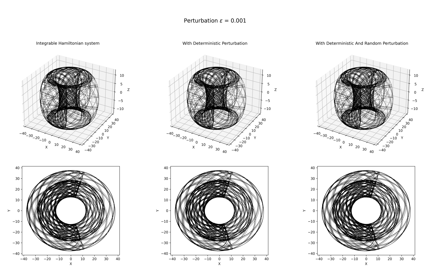
Figure 4. The first row of three plots represents the phase space trajectories of the solutions to the stochastic nearly integrable Hamiltonian system $\eqref{30}$, the nearly integrable Hamiltonian system $\eqref{31}$, and the corresponding integrable Hamiltonian system, respectively, under a perturbation strength $\epsilon=0.001$. The second row of plots shows the corresponding projections of the trajectories from the first row onto the X-Y plane.

At very small perturbations, the system closely resembles an integrable Hamiltonian system, see Fig 4. The invariant tori are well-preserved, and the trajectories in phase space exhibit regular, closed curves. Even with the introduction of deterministic and random perturbations, the system’s trajectory remains largely stable, with minimal impact from the stochastic terms.

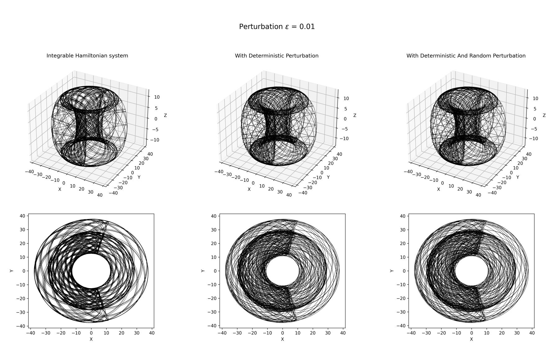
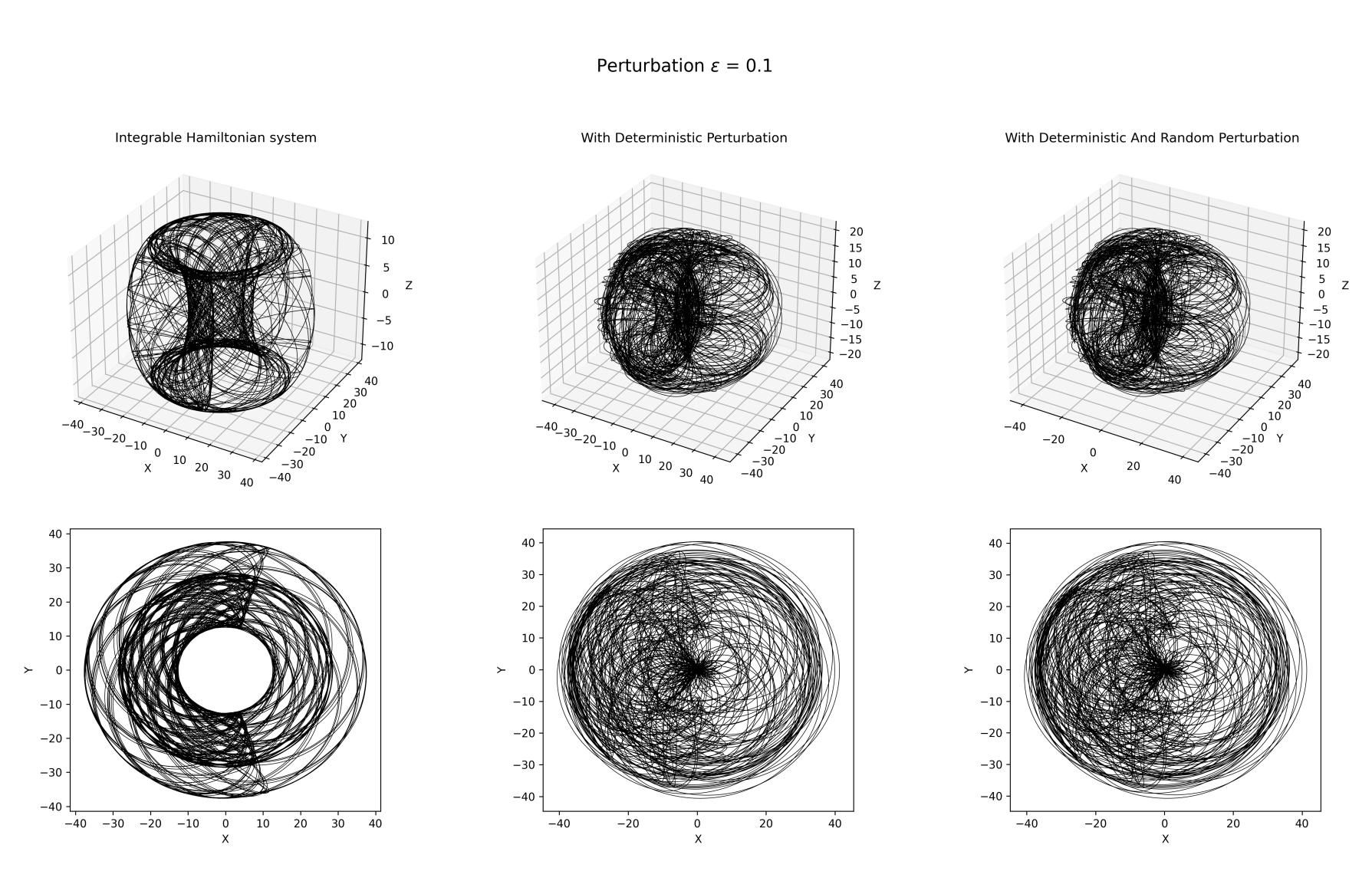
Figure 5. The comparison figure of Fig 4 when $\epsilon=0.01$ and $\epsilon=0.1$, respectively.

As the perturbation strength increases, the system’s trajectories begin to change, as shown in Fig 5. While the invariant tori are still present in phase space, the combined effects of deterministic and random perturbations lead to increased complexity in the trajectories. The stability of these trajectories gradually decreases, though they still exhibit quasi-periodic behavior. When the perturbation strength is further increased, the complexity grows significantly, with random perturbations introducing more fluctuations that result in chaotic trajectories. This indicates that when the perturbations are strong enough, the overall topological structure of the system becomes disrupted, ultimately leading to the destruction of the invariant tori.

From the results of these numerical simulations, we can observe that under small stochastic perturbations, the system’s trajectories generally evolve along deterministic paths, and the invariant tori are well-preserved. However, as the perturbation strength increases, the system’s trajectories become progressively more complex. The fluctuations introduced by random perturbations become more pronounced, especially when $\epsilon=0.1$, where the system exhibits stronger chaotic behavior.

Combining theoretical analysis with numerical simulation results, we can draw the conclusion that when the perturbation coefficient is small, the preservation of the invariant torus in the almost integrable stochastic Hamiltonian system can be guaranteed in a probabilistic sense. At this time, the trajectory of the system evolves along the solution of the deterministic Hamiltonian equation, and the probability of deviating from the most likely path decays exponentially. Although random perturbations introduce complexity, as long as the perturbations remain small, the basic structure of the system can still be retained.

References

• [1] V I Arnol’d, Proof of a theorem of A. N. Kolmogorov on the invariance of quasi-periodic motions under small perturbations of the hamiltonian., Russian Mathematical Surveys 18 (1963), no. 5, 9.
• [2] A. V. Balakrishnan, Applied functional analysis, Applications of Mathematics, vol. No. 3, Springer-Verlag, New York-Heidelberg, 1976. MR 470699
• [3] Xavier Bardina, Carles Rovira, and Samy Tindel, Onsager-Machlup functional for stochastic evolution equations, Ann. Inst. H. Poincaré Probab. Statist. 39 (2003), no. 1, 69–93. MR 1959842
• [4] Marco Carfagnini and Yilin Wang, Onsager–Machlup Functional for ${\rm SLE}_{\kappa}$ Loop Measures, Comm. Math. Phys. 405 (2024), no. 11, Paper No. 258. MR 4808252
• [5] Ying Chao and Jinqiao Duan, The Onsager-Machlup function as Lagrangian for the most probable path of a jump-diffusion process, Nonlinearity 32 (2019), no. 10, 3715–3741. MR 4002397
• [6] S.-N. Chow, Y. Li, and Y. Yi, Persistence of invariant tori on submanifolds in Hamiltonian systems, J. Nonlinear Sci. 12 (2002), no. 6, 585–617. MR 1938331
• [7] G. M. Constantine and T. H. Savits, A multivariate Faà di Bruno formula with applications, Trans. Amer. Math. Soc. 348 (1996), no. 2, 503–520. MR 1325915
• [8] Francesco Cordoni, Luca Di Persio, and Riccardo Muradore, Weak energy shaping for stochastic controlled port-Hamiltonian systems, SIAM J. Control Optim. 61 (2023), no. 5, 2902–2926. MR 4645664
• [9] Walter Craig and C. Eugene Wayne, Newton’s method and periodic solutions of nonlinear wave equations, Comm. Pure Appl. Math. 46 (1993), no. 11, 1409–1498. MR 1239318
• [10] Harald Cramér, Sur un nouveau théorème-limite de la théorie des probabilités, Actualités Scientifiques et Industrielles 736 (1938), 5–23 (French).
• [11] Jianbo Cui, Shu Liu, and Haomin Zhou, What is a stochastic Hamiltonian process on finite graph? An optimal transport answer, J. Differential Equations 305 (2021), 428–457. MR 4330908
• [12] Sylvain Delattre, Arnaud Gloter, and Nakahiro Yoshida, Rate of estimation for the stationary distribution of stochastic damping Hamiltonian systems with continuous observations, Ann. Inst. Henri Poincaré Probab. Stat. 58 (2022), no. 4, 1998–2028. MR 4492969
• [13] Amir Dembo and Ofer Zeitouni, Large deviations techniques and applications, second ed., Applications of Mathematics (New York), vol. 38, Springer-Verlag, New York, 1998. MR 1619036
• [14] Jean-Dominique Deuschel and Daniel W. Stroock, Large deviations, Pure and Applied Mathematics, vol. 137, Academic Press, Inc., Boston, MA, 1989. MR 997938
• [15] M. D. Donsker and S. R. S. Varadhan, Asymptotic evaluation of certain Markov process expectations for large time. I. II, Comm. Pure Appl. Math. 28 (1975), 1–47; ibid. 28 (1975), 279–301. MR 386024
• [16] by same author, Asymptotic evaluation of certain Markov process expectations for large time. III, Comm. Pure Appl. Math. 29 (1976), no. 4, 389–461. MR 428471
• [17] by same author, Asymptotic evaluation of certain Markov process expectations for large time. IV, Comm. Pure Appl. Math. 36 (1983), no. 2, 183–212. MR 690656
• [18] T. Dunker, W. V. Li, and W. Linde, Small ball probabilities for integrals of weighted Brownian motion, Statist. Probab. Lett. 46 (2000), no. 3, 211–216. MR 1745688
• [19] L. H. Eliasson, Perturbations of stable invariant tori for Hamiltonian systems, Ann. Scuola Norm. Sup. Pisa Cl. Sci. (4) 15 (1988), no. 1, 115–147. MR 1001032
• [20] Richard S. Ellis, Entropy, large deviations, and statistical mechanics, Grundlehren der mathematischen Wissenschaften [Fundamental Principles of Mathematical Sciences], vol. 271, Springer-Verlag, New York, 1985. MR 793553
• [21] M. I. Freidlin and A. D. Wentzell, Random perturbations of dynamical systems, second ed., Grundlehren der mathematischen Wissenschaften [Fundamental Principles of Mathematical Sciences], vol. 260, Springer-Verlag, New York, 1998, Translated from the 1979 Russian original by Joseph Szücs. MR 1652127
• [22] Leonard Gross, Measurable functions on Hilbert space, Trans. Amer. Math. Soc. 105 (1962), 372–390. MR 147606
• [23] Gilles Hargé, Limites approximatives sur l’espace de Wiener, Potential Anal. 16 (2002), no. 2, 169–191. MR 1881596
• [24] Nobuyuki Ikeda and Shinzo Watanabe, Stochastic differential equations and diffusion processes, second ed., North-Holland Mathematical Library, vol. 24, North-Holland Publishing Co., Amsterdam; Kodansha, Ltd., Tokyo, 1989. MR 1011252
• [25] Academician A. N. Kolmogorov, On conservation of conditionally periodic motions for a small change in hamilton’s function, Proceedings of the USSR Academy of Sciences 98 (1954), 527–530.
• [26] C. E. Koudjinan, A KAM theorem for finitely differentiable Hamiltonian systems, J. Differential Equations 269 (2020), no. 6, 4720–4750. MR 4104457
• [27] Joan-Andreu Lázaro-Camí and Juan-Pablo Ortega, Stochastic Hamiltonian dynamical systems, Rep. Math. Phys. 61 (2008), no. 1, 65–122. MR 2408499
• [28] Tiejun Li and Xiaoguang Li, Gamma-limit of the Onsager-Machlup functional on the space of curves, SIAM J. Math. Anal. 53 (2021), no. 1, 1–31. MR 4194315
• [29] Xue-Mei Li, An averaging principle for a completely integrable stochastic Hamiltonian system, Nonlinearity 21 (2008), no. 4, 803–822. MR 2399826
• [30] Yong Li and Yingfei Yi, Persistence of lower dimensional tori of general types in Hamiltonian systems, Trans. Amer. Math. Soc. 357 (2005), no. 4, 1565–1600. MR 2115377
• [31] S. Machlup and L. Onsager, Fluctuations and irreversible process. II. Systems with kinetic energy, Phys. Rev. (2) 91 (1953), 1512–1515. MR 57766
• [32] Sílvia Moret and David Nualart, Onsager-Machlup functional for the fractional Brownian motion, Probab. Theory Related Fields 124 (2002), no. 2, 227–260. MR 1936018
• [33] J Möser, On invariant curves of area-preserving mappings of an annulus, Nachr. Akad. Wiss. Göttingen, II (1962), 1–20.
• [34] L. Onsager and S. Machlup, Fluctuations and irreversible processes, Phys. Rev. (2) 91 (1953), 1505–1512. MR 57765
• [35] G. Popov, KAM theorem for Gevrey Hamiltonians, Ergodic Theory Dynam. Systems 24 (2004), no. 5, 1753–1786. MR 2104602
• [36] Jürgen Pöschel, Integrability of Hamiltonian systems on Cantor sets, Comm. Pure Appl. Math. 35 (1982), no. 5, 653–696. MR 668410
• [37] by same author, A KAM-theorem for some nonlinear partial differential equations, Ann. Scuola Norm. Sup. Pisa Cl. Sci. (4) 23 (1996), no. 1, 119–148. MR 1401420
• [38] Dietmar A. Salamon, The Kolmogorov-Arnold-Moser theorem, Math. Phys. Electron. J. 10 (2004), Paper 3, 37. MR 2111297
• [39] Ivan N Sanov, On the probability of large deviations of random variables, United States Air Force, Office of Scientific Research, 1958.
• [40] R. L. Stratonovič, On the probability functional of diffusion processes, Proc. Sixth All-Union Conf. Theory Prob. and Math. Statist. (Vilnius, 1960) (Russian), Gosudarstv. Izdat. Političesk. i Naučn. Lit. Litovsk. SSR, Vilnius, 1960, pp. 471–482. MR 205335
• [41] D. W. Stroock, An introduction to the theory of large deviations, Universitext, Springer-Verlag, New York, 1984. MR 755154
• [42] D. Talay, Stochastic Hamiltonian systems: exponential convergence to the invariant measure, and discretization by the implicit Euler scheme, Markov Process. Related Fields 8 (2002), no. 2, 163–198, Inhomogeneous random systems (Cergy-Pontoise, 2001). MR 1924934
• [43] Laszlo Tisza and Irwin Manning, Fluctuations and irreversible thermodynamics, Phys. Rev. (2) 105 (1957), 1695–1705. MR 94944
• [44] Liming Wu, Large and moderate deviations and exponential convergence for stochastic damping Hamiltonian systems, Stochastic Process. Appl. 91 (2001), no. 2, 205–238. MR 1807683
• [45] Xicheng Zhang, Stochastic flows and Bismut formulas for stochastic Hamiltonian systems, Stochastic Process. Appl. 120 (2010), no. 10, 1929–1949. MR 2673982
• [46] Xinze Zhang and Yong Li, Onsager-machlup functional for stochastic differential equations with time-varying noise, 2024.