Learning Accurate Models on Incomplete Data with Minimal Imputation

Abstract

Missing data often exists in real-world datasets, requiring significant time and effort for imputation to learn accurate machine learning (ML) models. In this paper, we demonstrate that imputing all missing values is not always necessary to achieve an accurate ML model. We introduce the concept of minimal data imputation, which ensures accurate ML models trained over the imputed dataset. Implementing minimal imputation guarantees both minimal imputation effort and optimal ML models. We propose algorithms to find exact and approximate minimal imputation for various ML models. Our extensive experiments indicate that our proposed algorithms significantly reduce the time and effort required for data imputation.

¹School of Electrical Engineering and Computer Science, Oregon State University, Corvallis, USA

1 Introduction

The performance of a machine learning (ML) model heavily depends on the quality of its training data. In real-world data, a major data quality issue is missing data, i.e., incomplete data. There are two prevalent approaches to address missing values in training data. The first approach involves deleting the data points or features with missing data. However, this method can lead to the loss of important information and introduce bias (Van Buuren, 2018).

Another popular approach is imputation in which ML practitioners replace missing values with correct ones (Little & Rubin, 2002; Le Morvan et al., 2021; Whang et al., 2023; Farhangfar et al., 2008; Andridge & Little, 2010; Śmieja et al., 2018; Williams et al., 2005; Pelckmans et al., 2005). However, accurate imputation is usually challenging and expensive as it often requires extensive collaboration with costly domain experts to find the correct values for missing data items. To reduce the cost of imputation, there has been a significant effort to devise models that predict accurate values for the missing data items (Le Morvan et al., 2021). Nonetheless, it is not clear if these models can deliver effective results and confidently replace domain experts in every domain, particularly in sensitive ones such as medical sciences. It also takes a great deal of time and effort to find, train, and validate proper models for the task at hand. Because their predicted values for missing data are estimations of correct values, using them over a dataset with many missing data items may introduce considerable inaccuracies or biases to the training data, resulting in learning an inaccurate or biased model. As accurate imputation models are often quite complex, e.g., DNNs (Mattei & Frellsen, 2019), it often takes a significant time to impute a large dataset with missing values using these models. Surveys indicate that ML practitioners spend about $80\%$ of their time preparing data, including imputing missing data (Krishnan et al., 2016; Neutatz et al., 2021).

There have been some efforts to eliminate the burden of data imputation for model training. Researchers have proposed stochastic optimization to find a model by optimizing the expected loss function over the probability distributions of missing data items in the training examples (Ganti & Willett, 2015). Similarly, in robust optimization, researchers minimize the loss function of a model for the imputation that brings the highest training loss while assuming certain distributions of the missing values (Aghasi et al., 2022). However, the distributions of missing data items are not often available. Thus, users may spend significant time and effort to discover or train these distributions, which may require the user to find the causes of missingness in the data and dependencies between the features. Additionally, for a given type of model, users must solve various and possibly challenging optimization problems for many possible (combinations of) distributions of missing values. More importantly, these methods reflect the uncertainty in the training data caused by missing values in the trained model. Hence, they deliver inaccurate models over the dataset with considerably many missing values.

There has been also some work on detecting cases where imputing missing data is not necessary to learn accurate models (Picado et al., 2020; Karlaš et al., 2020; Zhen et al., 2024). These methods check whether an accurate model can be learned without using training examples with missing features. Although these approaches are useful for some datasets and learning tasks, they ignore a majority of learning tasks in which imputing incomplete examples impacts the quality of the learned model.

To address these challenges, we introduce the concept of a minimal imputation set for an incomplete training dataset. This set represents the smallest group of missing data items that, once imputed, yields the same model as one trained on a fully imputed dataset. We propose novel and efficient methods to find minimal imputation for some of the popular ML models. By identifying and imputing only the minimal imputation set, this approach offers two key benefits. Firstly, in many domains, data imputation is performed using an oracle, meaning that the cost savings from imputation are directly proportional to the number of examples that can be avoided. Significant imputation costs are saved if the minimal imputation set is substantially smaller than the full set of incomplete examples. Secondly, ensuring the accuracy of imputed data is challenging, even when the imputation method is carefully selected and tailored. Thus, minimizing imputation also reduces the errors introduced into the original dataset. Moreover, compared to methods based on stochastic or robust optimization, a model trained with minimal imputation generally achieves higher accuracy, as this approach eliminates all relevant uncertainties in the training dataset.

Specifically, our contributions are:

• We formally define the concept of minimal imputation for learning over incomplete data.

• We prove that finding the minimal imputation for support vector machines (SVM) is NP-hard. We propose an efficient method with provable error bounds to approximate minimal imputation for SVM (Section 3).

• We prove that finding the minimal imputation for linear regression is NP-hard. We propose an efficient algorithm with provable error bounds to approximate minimal imputation for linear regression (Section 4).

• We conduct experiments to show cost savings in data cleaning and program execution time compared to imputing all missing data using multiple methods, including mean imputation, a KNN-based imputation algorithm, a diffusion model-based imputation method, and a benchmark framework. We also extend the comparison to diverse real-world datasets with inherent missing values, yielding results consistent with randomly corrupted datasets. Our studies show that our algorithms significantly reduce data imputation costs by finding minimal imputations (Section 5).

2 Background

Model Training

We model the input training data as a table where each row represents a training example, e.g., Table 1. One column in the table represents the label and others represent features of the examples. Given that the training data has $d$ features, we denote its features as $[\mathbf{z}_{1},\dots,\mathbf{z}_{d}]$. The values of each feature belong to the domain of the feature, e.g., real numbers. To simplify our analysis, we assume that all features share the same domain. Our results extend to other settings. A training set with $n$ examples is a pair of a feature matrix $\mathbf{X}=[\textbf{x}_{1},...,\textbf{x}_{n}]^{T}$ and a corresponding label vector $\textbf{y}=[y_{1},...,y_{n}]^{T}$. We denote each example with $d$ features in X as a vector $\textbf{x}_{i}=[x_{i1},...,x_{id}]$, where $x_{ij}$ represents the $j^{th}$ feature in the $i^{th}$ example. Taking a feature matrix $\mathbf{X}$, a label vector $\mathbf{y}$, a target function $f$, and a loss function $L$, the goal of training is to find an optimal model $\mathbf{w}^{*}$ that minimizes the training loss, i.e., $\mathbf{w}^{*}=\arg\min\limits_{\mathbf{w}\in\mathcal{W}}L(f(\mathbf{X},\mathbf{w}),\mathbf{y})$.

Table 1: A dataset for credit card approval prediction

Annual Income($)	Age	Decision
65000	30	1
10000	$null$	-1

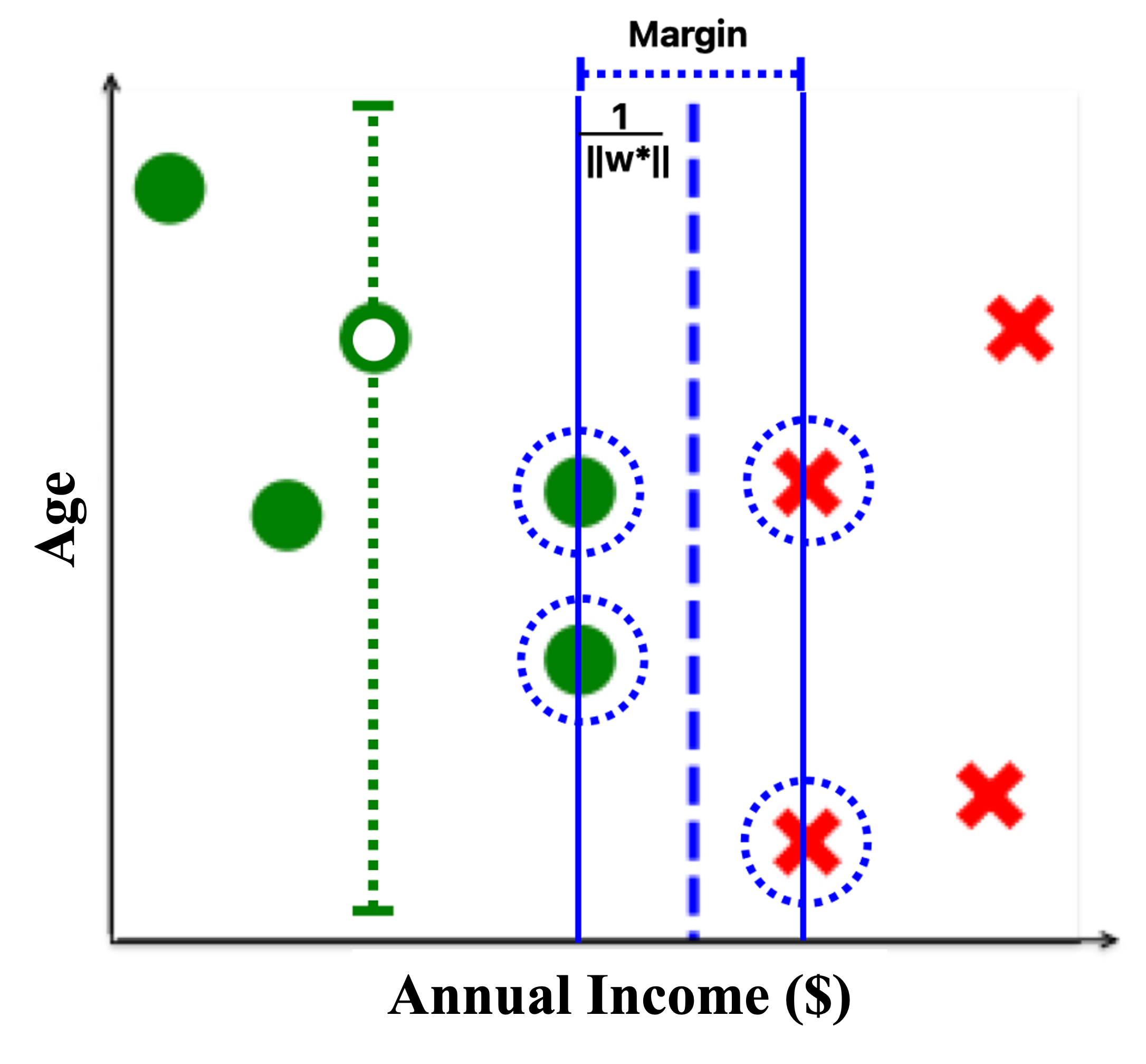
(a) Imputing missing values is not necessary at all

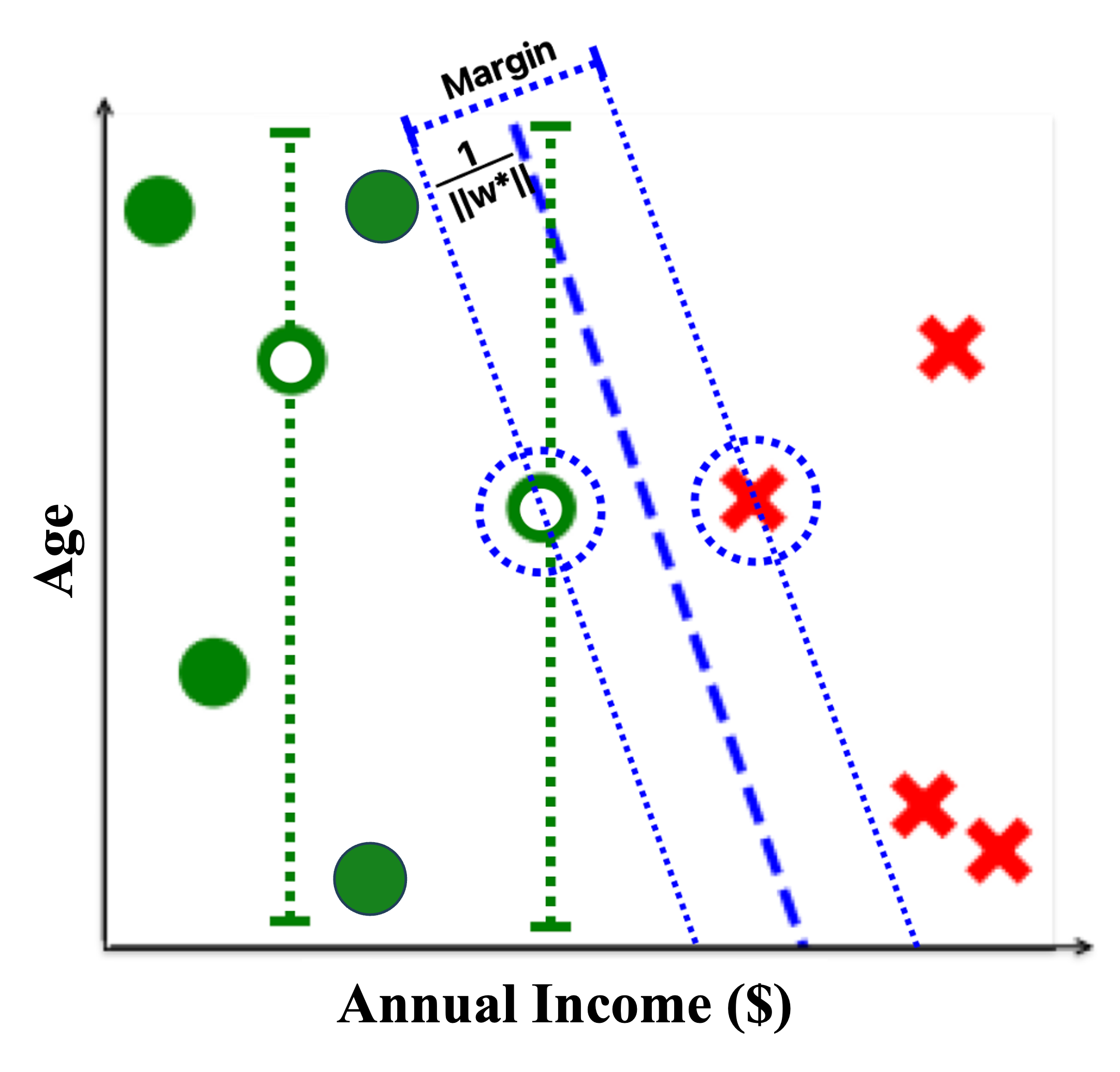
(b) Some missing values need imputation while others do not

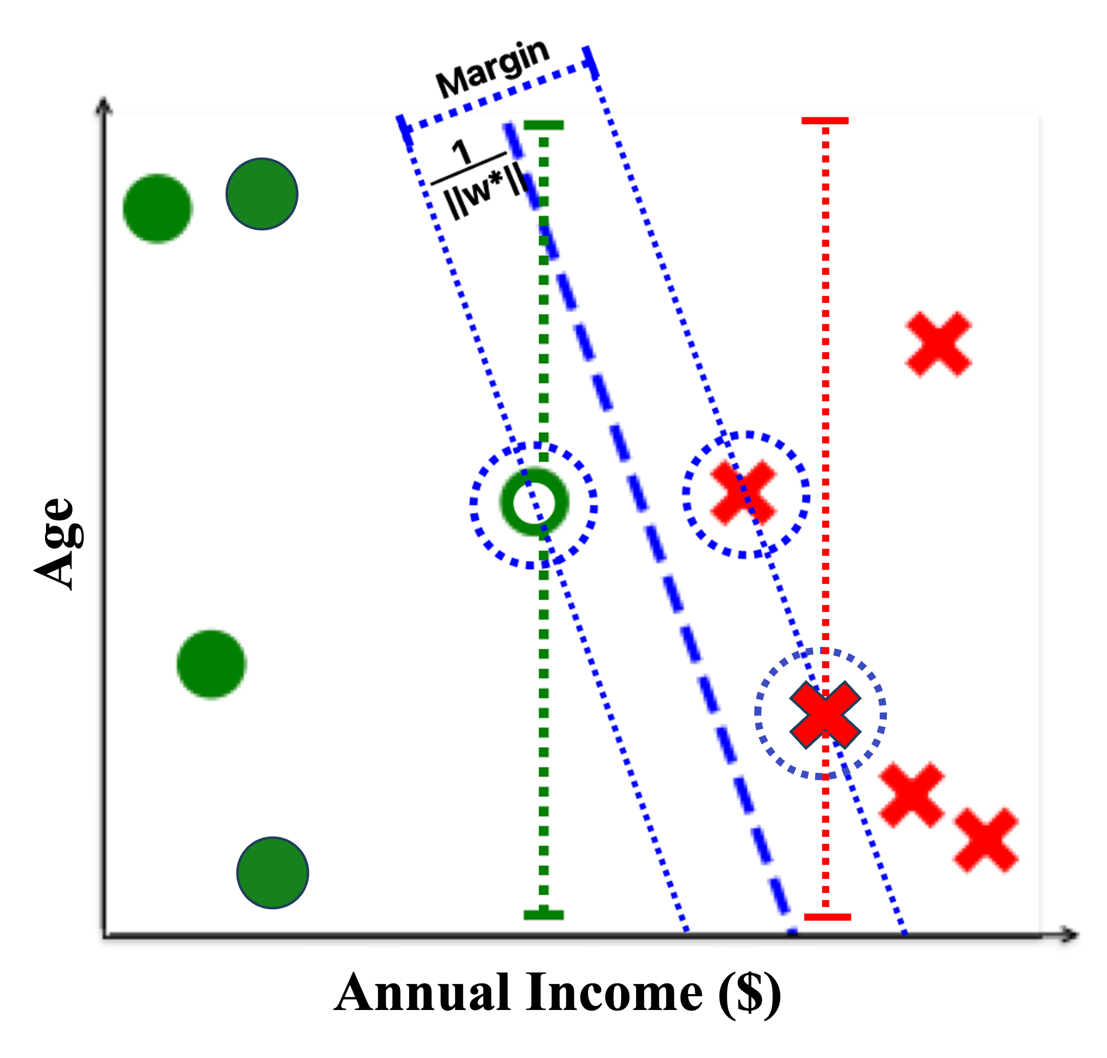
(c) All missing values need imputation

Figure 1: The necessity of missing data imputation varies

Missing values

Any $x_{ij}$ is a missing value if it is unknown (marked by null). An incomplete example is an example with at least one missing value. Similarly, an incomplete feature is a feature that contains at least one missing value. We use complete feature and complete example to refer to features and examples that are free of missing values. We further denote the set of all missing values in a feature matrix $\mathbf{X}$ as $MV(\mathbf{X})$, the set of incomplete examples as $MVE(\mathbf{X})$, and the set of incomplete features as $MVF(\mathbf{X})$. In this paper, we focus on the case that all missing values are in the feature matrix, and the label vector is complete.

Example 1

In Table 1, Age is an incomplete feature while Annual Income is a complete one. Similarly, the first training example is complete and the second training example is incomplete.

Repair

A repair is a complete version of an incomplete feature matrix where all missing values are imputed, i.e. replaced with values from their domains. More formally:

Definition 1

(Repair) $\textbf{X}^{r}$ is a repair to feature matrix X if 1) $dimension(\textbf{X}^{r})=dimension(\textbf{X})$, 2) $\forall x^{r}_{ij}\in\textbf{X}^{r},x^{r}_{ij}\neq\textit{null}$, and 3) $\forall x_{ij}\neq\textit{null}$, $x^{r}_{ij}=x_{ij}$.

Given the repair $\textbf{X}^{r}$ of the feature matrix X, we denote the repair, i.e., imputation, of example $\textbf{x}_{i}$ in X by $\textbf{x}_{i}^{r}$.

Example 2

In Table 1, replacing the missing data with a value,e.g., $45$, produces a repair. However, deleting the Age feature, which eliminates the missing value, is not a repair since it changes $dimension(\textbf{X})$.

Possible Repairs

Since the domains of features often contain numerous or infinite values, an incomplete feature matrix usually has numerous or infinitely many repairs. We denote this set of all possible repairs of a feature matrix X as $\textbf{X}^{R}$.

Example 3

Figures 1(a), 1(b), and 1(c) display three sets of training examples with missing Age values. The green and red dashed lines represent the range of possible values for the incomplete feature (denoted by empty circles). In Figure 1(a), the incomplete examples do not intersect the SVM margins (outlined by the solid blue lines) with any possible repair to the feature matrix ($\textbf{X}^{r}\in\textbf{X}^{R}$) and, therefore, are not support vectors. As a result, the model (decision boundary: blue dashed line) remains optimal across all repairs, and a certain model ($\textbf{w}^{*}$) exists. In this scenario, imputing missing data is unnecessary. However, in Figures 1(b) and 1(c), since at least one incomplete example may intersect the blue rectangle with some repairs of the feature matrix, the optimal model changes from one repair to another, and a certain model does not exist. In this scenario, data imputation is necessary to achieve an accurate model.

Certain Models

Researchers have defined the concept of certain models to determine the necessity of imputing missing data for learning (Zhen et al., 2024).

Definition 2

(Certain Model) A model $\textbf{w}^{*}$ is a certain model for target function $f$ over training set $(\mathbf{X},\mathbf{y})$ if:

$$\forall\textbf{X}^{r}\in\textbf{X}^{R},\textbf{w}^{*}=\mathop{\arg\min}\limits_{\textbf{w}\in\mathcal{W}}L(f(\textbf{X}^{r},\textbf{w}),\textbf{y})$$ (1)

Intuitively, a certain model is optimal, i.e., minimizes the training loss, for all repairs to the incomplete feature matrix. Thus, if a certain model exists, one can learn an accurate model over the dataset without any costly imputation as training over any imputation of the dataset, e.g., using randomly selected values, will deliver the same accurate model. However, given the restrictive definition, certain models do not often exist (Zhen et al., 2024). In this paper, we find the minimal amount of data imputation of an incomplete training set such that the resulting dataset has a certain model.

3 Minimal Imputation for SVM

In SVM, support vectors are the training examples building the optimal model that minimizes the loss function $L(f(\textbf{X},\textbf{w}),\textbf{y})=\frac{1}{2}||\textbf{w}||^{2}_{2}+C\sum_{i=1}^{n}max\{0,1-y_{i}\textbf{w}^{T}\textbf{x}_{i}\}$. $(\textbf{x}_{i},y_{i})$ is a support vector if $y_{i}\textbf{w}^{T}\textbf{x}_{i}\leq 1$. Intuitively, an incomplete example needs to be imputed if it determines the optimal model, i.e., if it is a support vector in some repairs. Conversely, an incomplete example does not need to be imputed if it is not a support vector in any repair. Therefore, we formally define the minimal imputation set on an example-wise basis as the smallest set of incomplete examples that, when imputed, guarantees an accurate SVM model.

Definition 3

(Minimal imputation set) A set of incomplete examples $\mathbf{S}$ in the training set $(\mathbf{X},\mathbf{y})$ is a minimal imputation set for learning SVM with regularization parameter $C$ if we have: 1) a certain model exists upon imputing all missing values $\mathbf{S}$ and 2) there is no set $\mathbf{S^{\prime}}$ satisfying condition (1) such that $|\mathbf{S^{\prime}}|<|\mathbf{S}|$ where $|\mathbf{S}|$ denotes the cardinality of $\mathbf{S}$.

We denote the minimal imputation set for SVM with regularization parameter $C$ over the training set $(\mathbf{X},\mathbf{y})$ as $\mathbf{S}_{min}(\mathbf{X},\mathbf{y},C)$. We have the following property for the minimal imputation set.

Theorem 1

(Uniqueness of the minimal imputation set) Given the training set training set $(\mathbf{X},\mathbf{y})$ and regularization parameter $C$, $\mathbf{S}_{min}(\mathbf{X},\mathbf{y},C)$ is unique.

3.1 Finding minimal imputation

Let $SV(\mathbf{X^{r}},\mathbf{y},C)$ be the set of support vectors for the optimal SVM model with regularization parameter $C$ over a repair of the training set ($\mathbf{X},\mathbf{y}$). The following theorem formalizes an important property of the minimal imputation set for SVM discussed at the beginning of this section.

Theorem 2

Given the training set $(\mathbf{X},\mathbf{y})$ and regularization parameter $C$, at least one imputation of every example in $S_{min}(\mathbf{X},\mathbf{y},C)$ is a support vector in a repair of $\mathbf{X}$, i.e.,

$$S_{min}(\mathbf{X},\mathbf{y},C)=\{\mathbf{x}_{i}|\exists\mathbf{X}^{r}\in\mathbf{X}^{R},\mathbf{x}^{r}_{i}\in SV(\mathbf{X},\mathbf{y},C)\}$$

where $\mathbf{x}^{r}_{i}$ is the corresponding repair of $\mathbf{x}_{i}$ in $\mathbf{X}^{r}$.

To determine if an incomplete example belongs to the minimal imputation set, one could materialize every repair of the feature matrix and check if the incomplete example is a support vector for any of them. However, this process can be extremely inefficient due to the often large number of repairs. Assume that each missing value $x_{ij}$ is bounded by an interval based on its domain.

Definition 4

(Edge repair) $\mathbf{X}^{e}$ is an edge repair to $\mathbf{X}$ if for every missing values $x_{ij}$, $x_{ij}^{e}=x_{ij}^{min}$ or $x_{ij}^{min}$. $\mathbf{X}^{E}$ denotes the set of all edge repairs of $\mathbf{X}$.

Theorem 3 shows that we can use only the edge repairs instead of all repairs to check if an incomplete example belongs to the minimal imputation set.

Theorem 3

Given training set $(\mathbf{X},\mathbf{y})$ and regularization parameter $C$, an incomplete example $\mathbf{x}_{i}$ belongs to the minimal imputation set $S_{min}(\mathbf{X},\mathbf{y},C)$ if and only if there is at least one edge repair $\mathbf{X}^{e}$ of $\mathbf{X}$ such that $\mathbf{x}_{i}^{e}\in SV(\mathbf{X}^{e},\mathbf{y},C)$ where $\mathbf{x}_{i}^{e}$ is the imputation of $\mathbf{x}_{i}$.

Based on Theorem 3, we can find the minimal imputation set by following these steps: 1) Initialize an empty minimal imputation set, $S_{min}$. 2) Iterate over each incomplete example $\mathbf{x}_{i}$. At each iteration, materialize all edge repairs $\mathbf{X}^{e}\in\mathbf{X}^{E}$, and check if $\mathbf{x}_{i}$ is a support vector for any of the edge repairs. If it is, add $\mathbf{x}_{i}$ to $S_{min}$, and 3) Finally, return the minimal imputation set $S_{min}$.

Despite this optimization, finding the minimal imputation set remains an NP-hard problem, as determining whether an incomplete example $\mathbf{x}_{i}$ is a support vector in at least one edge repair is NP-hard, as established in Theorem 4.

Theorem 4

The problem of determining whether there exists an edge repair that makes a given incomplete example $\mathbf{x}_{i}$ a support vector in SVM is NP-hard. Consequently, listing all incomplete examples that can be support vectors in at least one repair is also NP-hard.

3.2 Approximating Minimal Imputation

In the case that finding the exactly minimal imputation set for SVM is NP-hard, we propose an efficient approximation method.

Instead of exhaustively checking all possible edge repairs to the feature matrix to determine if the target incomplete example ($\mathbf{x}_{i}$) is a support vector for any of the edge repairs, we construct an edge repair that approximately maximizes the likelihood of $\mathbf{x}_{i}$ being a support vector by individually scanning the missing values. More precisely, the process starts with a random edge repair to the feature matrix and then iterates over each missing value. During each iteration, all other repairs are fixed except for one missing value, $x_{pq}$. We then update $x_{pq}$ to either $x_{pq}^{\min}$ or $x_{pq}^{\max}$, whichever minimizes $y_{i}\mathbf{w}^{T}\mathbf{x}_{i}$, thereby maximizing the likelihood that $\mathbf{x}_{i}$ becomes a support vector. By the end of the iteration, we obtain an edge repair, $\mathbf{X}^{e}$, that approximately maximizes the likelihood of $\mathbf{x}i$ being a support vector. If $\mathbf{x}_{i}$ is not a support vector in the model trained with $\mathbf{X}^{e}$, we conclude that $\mathbf{x}i$ is not part of the minimal imputation set $S_{min}$. Algorithm 1 demonstrates this approach.

Algorithm 1 Approximating minimal imputation for SVM efficiently

 $S_{min}\leftarrow[\quad]$

 $MV(X)\leftarrow\text{set of missing values}$

 $MVE(\textbf{x})\leftarrow\text{set of incomplete examples}$

 $\mathbf{X}^{e}\leftarrow\text{a random edge repair to the feature matrix }\mathbf{X}$

 for $\mathbf{x}_{i}\in MV(\mathbf{x})$ do

  for $x_{pq}\in MV$ do

   $\mathbf{X}^{e}(x_{pq}^{min}),\mathbf{X}^{e}(x_{pq}^{max})\leftarrow\text{two edge repairs}${only replacing $x_{pq}$ in $\mathbf{X}^{e}$ by its two edge repairs}

   $\mathbf{w}_{1}\leftarrow SVM(\mathbf{X}^{e}(x_{pq}^{min}),\mathbf{y})$

   $\mathbf{w}_{2}\leftarrow SVM(\mathbf{X}^{e}(x_{pq}^{max}),\mathbf{y})$

   if $y_{i}\textbf{w}_{1}^{T}\leq y_{i}\textbf{w}_{2}^{T}$ then

    $\mathbf{X}^{e}\leftarrow\mathbf{X}^{e}(x_{pq}^{min})$

   end if

  end for

  $\mathbf{w}\leftarrow SVM(\mathbf{X}^{e},\mathbf{y})$

  if $y_{i}\textbf{w}^{T}\textbf{x}_{i}\leq 1$ then

   $S_{min}\leftarrow S_{min}.add(\mathbf{x}_{i})$

  end if

 end for

 $res\leftarrow S_{min}$

Since we modify only one missing value at each iteration, the datasets used to train adjacent models ($\mathbf{w}_{1}$ and $\mathbf{w}_{2}$) differ by just a single value in the feature matrix. Therefore, instead of fully retraining a new model for each iteration, we can leverage incremental and decremental learning to significantly reduce computational costs. Specifically, given an SVM model $\mathbf{w}$ and its corresponding feature matrix $\mathbf{X}$, if we change only one value $x_{ij}$ to create a new feature matrix $\mathbf{X}^{\prime}$, we can obtain the updated SVM model $\mathbf{w}^{\prime}$ for $\mathbf{X}^{\prime}$ through incremental and decremental learning with a time complexity that is one order of magnitude lower than that required for fully retraining the model (Laskov et al., 2006; Cauwenberghs & Poggio, 2000).

Next. we analyze the accuracy of Algorithm 1. First, Algorithm 1 does not return any incomplete example that does not belong to the minimal imputation set of the training data, i.e., no false positives.

Theorem 5

Every example returned by Algorithm 1 over training set $(\mathbf{X},\mathbf{y})$ and regularization parameter $C$ belongs to $S_{min}(\mathbf{X},\mathbf{y},C)$.

However, Algorithm 1 may miss some examples that are in the minimal imputation set, i.e., false negative. The following theorem bounds the probability of such an event.

Theorem 6

Let $g(x_{ij})$ denote the probability density function of the ground-truth value for missing value $x_{ij}$ in incomplete training set $X$. If missing values in $X$ are independent, the probability that an incomplete example $\mathbf{x}_{i}$ that belongs to the minimal imputation set of $X$ but not returned by Algorithm 1 is:

$$p(\mathbf{x}_{i})=\frac{\idotsint_{min(x_{ij}^{visited})}^{max(x_{ij}^{visited})}\prod_{x_{ij}\in MV}g(x_{ij})\,dx_{ij}}{\idotsint_{x_{ij}\in MV}\prod_{x_{ij}\in MV}g(x_{ij})}$$

where $x_{ij}^{visited}$ is a set containing the value(s) we have used for $x_{ij}$ in Algorithm 1. $x_{ij}^{visited}$ can either be $\{x_{ij}^{min}\}$, $\{x_{ij}^{max}\}$, or $\{x_{ij}^{min},x_{ij}^{max}\}$. $min(x_{ij}^{visited})$ and $max(x_{ij}^{visited})$ represent the minimum and maximum values in the set, respectively.

Theorem 6 suggests that the more edge repairs Algorithm 1 covers, the greater the likelihood that $S_{min}$ includes all incomplete examples. For instance, consider a dataset with two missing values, $x_{ij}$ and $x_{pq}$, where the ground truth of each missing value follows a uniform distribution between $-1$ and $1$. Suppose Algorithm 1 samples three edge repairs: (1) $x_{ij}=-1$ and $x_{pq}=-1$, (2) $x_{ij}=-1$ and $x_{pq}=1$, and (3) $x_{ij}=1$ and $x_{pq}=-1$. In this case, the probability that Algorithm 1 captures all incomplete examples in the minimal imputation set is $50\%$.

4 Minimal Imputation for Linear Regression

We define the minimal imputation for linear regression as follows.

Definition 5

Given the training set $(\mathbf{X},\mathbf{y})$, a set of incomplete features in $\mathbf{X}$, denoted as $\mathbf{S}_{min}(\mathbf{X},\mathbf{y})$, is a minimal imputation set for $(\mathbf{X},\mathbf{y})$ if we have: 1) a certain model exists upon imputing all missing values in the $\mathbf{S}_{min}(\mathbf{X},\mathbf{y})$, and 2) there is no set $\mathbf{S}$ satisfying condition (1) and $|\mathbf{S}|<|\mathbf{S}_{min}|$.

Definition’s Intuition

A minimal set for imputations refers to the smallest set of incomplete features that are necessary to impute to ensure an accurate linear regression model.

In linear regression, the optimal linear regression model $\mathbf{w}^{*}$ consists of the set of linear coefficients for feature vectors. A feature $\mathbf{z}_{i}$ is considered relevant if the corresponding linear coefficient in the optimal model $w_{i}^{*}$ is not zero, and it is irrelevant if $w_{i}^{*}$ equals zero. Intuitively, an incomplete feature needs to be imputed if it is relevant (i.e., it plays a role in the optimal model) and does not need to be imputed if it is irrelevant. However, traditional statistical tools, such as the chi-square test, require complete distributions for each feature to assess correlations, which is challenging in the presence of missing values. Therefore, identifying the minimal set of incomplete features for imputation involves determining which features are irrelevant, regardless of how other incomplete features are handled. Note that the minimal imputation set for linear regression is not necessarily unique.

Theorem 7

There is a training set with multiple minimal imputation sets for linear regression. Also, if all features in all repairs of the training set $(\mathbf{X},\mathbf{y})$ are linearly independent, the minimal imputation set for linear regression over $(\mathbf{X},\mathbf{y})$ is unique.

4.1 Finding Minimal Imputation

A baseline algorithm for finding the minimal imputation set is: (1) learn linear regression models with each possible repair individually, and (2) identify the set $\mathbf{S}_{min}$ with the smallest size such that all repairs to features not in $\mathbf{S}_{min}$ share at least one mutual optimal model. However, the set of possible repairs is often large, making the process of learning models from all repairs potentially very slow. In our search for a more efficient method, we note that finding the minimal imputation set for linear regression is intractable, as established in Theorem 8

Theorem 8

Finding the minimal imputation set for linear regression over a training set is NP-hard.

Therefore, we aim to develop efficient algorithms for finding the minimal imputation set without materializing all repairs.

4.2 Approximating Minimal Imputation Efficiently

We first propose an equivalent problem in Theorem 9, based on a variant of the well-known sparse linear regression problem (Bruckstein et al., 2009).

Theorem 9

Finding the minimal imputation set for linear regression over the training set $(\mathbf{X},\mathbf{y})$ is equivalent to:

$$\begin{array}[]{ll}\mathop{\min}\limits_{\mathbf{w}\in\mathcal{W}}T_{MVF(\mathbf{X})}(\mathbf{w})\\ \text{subject to}\quad\mathbf{w}=\mathop{\arg\min}||\mathbf{X}^{r}\mathbf{w}-\mathbf{y}||^{2}_{2},\forall\mathbf{X}^{r}\in\mathbf{X}^{R}\end{array}$$

where $T_{MVF(\mathbf{X})}(\mathbf{w})$ is the number of non-zero linear coefficient in $\mathbf{w}$ whose corresponding feature is complete, i.e., $T_{MVF(\mathbf{X})}(\mathbf{w})=|\{\mathbf{z}_{i}\in MVF(\mathbf{X})|w_{i}!=0\}|$

The key distinction between our problem and sparse linear regression lies in their objectives: sparse linear regression seeks to minimize the number of non-zero coefficients across all features, whereas our problem focuses on minimizing the number of non-zero coefficients only among incomplete features.

Orthogonal Matching Pursuit (OMP) provides an efficient approximation for solving the sparse linear regression problem (Wang et al., 2012). Essentially, this greedy algorithm begins with an empty solution set and initializes the regression residual to the label vector. In each iteration, the algorithm selects the feature most relevant to the current residual (i.e., having the largest dot product), adds it to the solution set, retains a linear regression model, and updates the residual accordingly. The program stops when the regression residue is sufficiently small. Therefore, OMP will return a subset of features (the solution set) that are sufficient to achieve an optimal linear regression model.

In this paper, we propose a variant of OMP, as outlined in Algorithm 2, to find minimal imputation for linear regression. Our algorithm has two major differences compared to the conventional OMP. Firstly, we include all complete features in the regression at the initialization, ensuring that we minimize the number of non-zero coefficients only among incomplete features. Secondly, we define our stopping condition by the maximum relevance (cosine similarity) between the feature and the label being smaller than or equal to a user-defined threshold, instead of relying on a near-zero regression residue. This approach enables our algorithm to work with general datasets without requiring the assumption of an underdetermined linear system, which is typically necessary in conventional OMP.

Algorithm 2 Approximating minimal imputation for linear regression efficiently

 $S_{min}\leftarrow[\quad]$

 $MVF(\textbf{z})\leftarrow\text{set of incomplete features}$

 $Complete(\textbf{z})\leftarrow\text{set of complete features}$

 $\textbf{r}\leftarrow LR(Complete(\mathbf{z}),\mathbf{y})$ {The residue vector from performing linear regression between complete features and label}

 $\epsilon\leftarrow\text{a user-defined threshold for stopping condition}$

 $MaxCosSim\leftarrow\mathop{\max}_{\mathbf{z}\in MVF(\textbf{z})}|cos(\mathbf{z},\mathbf{r})|$

 while $MaxCosSim\leq\epsilon$ do

  $S_{min}\leftarrow S_{min}.add(\mathop{\arg\max}_{\mathbf{z}\in MVF(\textbf{z})}|cos(\mathbf{z},\mathbf{r})|)$

  $\textbf{r}\leftarrow LR(Complete(\mathbf{z})\cup S_{min},\mathbf{y})$

  $MaxCosSim\leftarrow\mathop{\max}_{\mathbf{z}\in MVF(\textbf{z})}|cos(\mathbf{z},\mathbf{r})|$

 end while

 $res\leftarrow S_{min}$

The time complexity of the algorithm is $\mathcal{O}(T_{train}\cdot|MVF(\mathbf{z})|)$, making it significantly more efficient than the baseline algorithm, which trains models over all repairs individually and has a time complexity of $\mathcal{O}(T_{train}\cdot|\mathbf{X}^{R}|)$. If a gradient descent algorithm is used, Algorithm 2 has a time complexity of $\mathcal{O}(n\cdot d^{3})$, where $n$ is the number of training examples and $d$ is the number of features. In cases where $n<d^{2}$, the time complexity can be reduced to $\mathcal{O}(n\cdot d^{2}+n^{2}\cdot d)$ under certain conditions by applying incremental learning techniques based on the Sherman-Morrison formula, as outlined in the appendix.

While the approximation of the minimal imputation set does not depend on the probability distribution of the missing values, if the probability distributions of the missing values are known, the approximation rate can be improved under certain conditions, as demonstrated in Theorem 10. This approximation rate provides the probability that the approximation is correct, meaning the incomplete features identified by Algorithm 2 belong to at least one minimal imputation set. Note that the minimal imputation set is not necessarily unique for linear regression, as discussed in Theorem 7.

Theorem 10

The first $k$ incomplete features added to $S_{min}$ in Algorithm 2 for input training set $(\mathbf{X},\mathbf{y})$ belong to the minimal imputation set of $(\mathbf{X},\mathbf{y})$ with a probability of at least $1-1/n$, provided the following conditions are met: 1) $\mu<1/(2k-1)$, 2) the missing values in the dataset follow independent zero-mean normal distributions, i.e., $\forall x_{ij}=\text{null}$, $x_{ij}\sim\mathcal{N}(0,\sigma^{2}_{ij})$, and 3) all linear coefficients ($w_{i},\mathbf{z}_{i}\in MVF(\mathbf{X})$) for incomplete features satisfy:

$$|w_{i}|\geq\frac{2\sum_{x_{ij}=null}\sigma_{ij}\sqrt{n+2\sqrt{nlogn}}}{1-(2k-1)\mu}$$

where $\mu$ is the mutual incoherence defined by

$$\mu=\mathop{\max}\limits_{i\neq j}|\mathbf{z_{i}}^{T}\mathbf{z_{j}}|$$

Given the probability distribution of missing values, the smaller the mutual incoherence, the more incomplete features are guaranteed to be correctly included in $S_{min}$.

5 Experimental Evaluation

Table 2: Details of Real World Dataset containing missing values

Data Set	Task	Features	Training Examples	Missing Factor
Breast Cancer	Classification	10	559	1.97%
Water-Potability	Classification	9	2620	39.00%
Online Education	Classification	36	7026	35.48%
Air Quality	Regression	12	7344	90.80%
Communities	Regression	1954	1595	93.67%

We conducted experiments on a diverse set of real-world datasets, comparing our algorithms with one natural baseline, a KNN imputation method, a diffusion model-based imputation method, and the benchmark method ActiveClean. Our results demonstrate significant reductions in data cleaning costs without compromising ML model performance while maintaining competitive program execution times.

5.1 Experimental Setup

Table 3: SVM: Performance Comparison on Real-World Datasets with Original Missing Values

Data Set	Examples Imputed		Time (Sec)					Accuracy(%)
	MI/KI/DI	AC	MI	KI	DI	AC	MICE	MI	KI	DI	AC	MICE
Breast Cancer	11	10	0.004	0.004	1261	0.001	0.148	66.67	66.67	66.67	50.55	66.67
Water Potability	1022	30	0.04	0.38	4718	0.40	0.439	60.53	60.53	49.15	49.15	60.53
Online Education	2427	20	0.05	2.65	8816	3.30	2.631	49.15	60.53	65.23	52.02	65.14

Table 4: SVM: Performance Comparison on Real-World Datasets with Original Missing Values

Data Set	Examples Imputed	Time (Sec)				Accuracy(%)
	MiniI	MiniIM	MiniIK	MiniID	MiniIMICE	MiniIM	MiniIK	MiniID	MiniIMICE
Breast Cancer	4	0.021	0.022	1108	0.141	66.66	66.66	67.86	66.66
Water Potability	787	11.38	11.37	4622	11.633	60.53	60.53	62.80	60.53
Online Education	2151	134.1	134.14	8897	136.15	60.53	60.53	64.83	65.23

Table 5: Linear Regression: Performance Comparison on Real-World Datasets with Original Missing Values

Data Set	Features Imputed	Time (Sec)				Mean Squared Error (MSE)
	MI/KI/DI	MI	DI	KI	MICE	MI	DI	KI	MICE
Air Quality	4	0.003	18372	1.763	2.46	72.88	5.825	64.17	5.923
Communities	25	0.141	null	9.691	33475	0.004	null	0.549	0.024

Table 6: Linear Regression: Performance Comparison on Real-World Datasets with Original Missing Values

Data Set	Features Imputed	Time (Sec)				Mean Squared Error (MSE)
	MiniI	MiniIM	MiniIK	MiniID	MiniIMICE	MiniIM	MiniIK	MiniID	MiniIMICE
Air Quality	2	0.28	1.06	14976	1.218	65.47	59.53	5.817	5.74
Communities	20	0.12	10.00	null	28863	0.0512	0.4093	null	0.026

5.1.1 Hardware and Platform

The experiments were conducted on an x86_64 machine equipped with 30 Intel(R) Xeon(R) CPU E5-2670 v3 cores at 2.30GHz and 512GB RAM, running in a VMware virtualized environment with two NUMA nodes and a total of 30MB L3 cache. However, this hardware lacks sufficient computational resources for training and performing imputation with the diffusion model introduced in Section 5.1.3. Instead, for the diffusion model baseline, we use an Nvidia DGX2 system with one Nvidia Tesla V100 GPU (32 GB VRAM) and 20 CPU cores from 2.70 GHz Intel Xeon Platinum 8168 CPUs with a 33MB cache.

5.1.2 Real-world Datasets with Original Missing Values

We also experimented with eight real-world datasets that originally contained missing values, selected from diverse domains with various missing factors, where missing factor represents the ratio of incomplete examples to the total examples. Table 2 summarizes these datasets. For preprocessing, we dropped examples with missing labels and used sklearn’s OneHotEncoder for categorical attributes.

Water Potability

This dataset includes data on substances in freshwater, predicting whether water is potable or not (Kadiwal, 2021).

Breast Cancer

This dataset contains characteristics of potential cancerous tissue, predicting whether it is benign or malignant (Wolberg, 1992).

Online Education

The dataset contains survey responses on online education, predicting whether students prefer cellphones or laptops for the courses (Vanschoren et al., 2013).

Air Quality

The dataset contains instances of hourly averaged responses from an array of chemical sensors embedded in an Air Quality Chemical Multisensor Device (Vito, 2016). Given air-composition measurements, the regression task is to predict hourly Temperature.

Communities-Crimes

The data contains socio-economic and crime data from the US Census and FBI. The regression task is to predict the total number of violent crimes per 100K population (Redmond, 2009).

5.1.3 Algorithms for Comparison

In our experiments, we include two natural imputation baselines, a diffusion model-based imputation algorithm, and a benchmark algorithm for comparison.

Active Clean (AC)

ActiveClean (Krishnan, Sanjay et al., 2018; Krishnan et al., 2016) aims to reduce the number of examples for data repairing. The method integrates data repair with model training using stochastic gradient descent. In each iteration, a batch of examples is sampled, cleaned, and then used to update the model parameters via their gradients. While this approach reduces data repairing costs by prioritizing the sampling and repair of influential examples, it remains unclear whether the repaired data guarantees an accurate model, as not all examples are sampled and used in gradient updates across iterations.

KNN-Imputer (KI)

This method predicts the values of missing items based on observed examples using a KNN classifier  (Mattei & Frellsen, 2019).

Diffusion model based Imputation (DI)

We include TabCSDI (Zheng & Charoenphakdee, 2022), which trains a diffusion model to model, impute, and detokenize (for categorical features) missing values specifically for tabular data. In our experiments, we provide incomplete examples and features as input for diffusion model imputation for SVM and linear regression, respectively.

Mean Imputation (MI)

Each missing feature value is imputed with the mean value of that feature (Mattei & Frellsen, 2019).

Multiple Imputation by Chained Equations (MICE)

MICE (Van Buuren & Groothuis-Oudshoorn, 2011) predicts the values of missing items by iteratively modeling each variable with missing data as a function of the other variables in the dataset. Generate multiple imputed values for missing entries using regression-based models in a chained process, capturing the uncertainty of missing data while preserving relationships between variables. Later, we use the imputed complete data for downstream tasks such as SVM classification and linear regression.

5.1.4 Metrics

We evaluate all algorithms on a held-out test set with complete examples. We use accuracy as a metric for classification tasks. Accuracy reflects the percentage of total correct class predictions therefore higher accuracy is preferred. For regression tasks, we use mean squared error (MSE). MSE measures the average squared difference between actual and predicted values. Therefore, a lower MSE is preferred. We also study the algorithms’ data cleaning efforts in terms of program execution time and the number of examples cleaned.

5.2 Results on Real-world Datasets with Inherent Missingness

Tables 4 and 6 present a performance comparison between our minimal imputation method and other approaches for SVM and linear regression, respectively, across datasets with original missing values. MiniIM and MiniIK, refer to applying mean imputation and KNN imputation, respectively, over the minimal imputation set. We report null for the time and accuracy results from DI on the Communities dataset because the baseline runs for more than 24 hours without returning imputation results. The results show that identifying and imputing only the minimal imputation set enables us to clean a smaller subset of incomplete examples. If an oracle is used for data imputation, the cost savings are proportional to the number of examples that can be avoided. In contrast, if model-based imputation is used—where most of the time is spent training the imputation model—the cost savings are reduced. Nevertheless, the minimal imputation method still provides some cost savings and, more importantly, guarantees that downstream model accuracy is not compromised. This is supported by a pairwise comparison between the accuracies of MiniIK and KI, as well as MiniIM and MI. Similarly, MiniID and DI, as well as MiniIMICE and MICE, yield comparable results, where the accuracies are very close to each other. This demonstrates that imputing only the minimal set ensures that downstream machine learning models achieve accuracy comparable to imputing all missing values using the same imputation method.

Compared to the benchmark method, ActiveClean, which also aims to reduce data cleaning operations, the minimal imputation method results in fewer imputed examples than ActiveClean in the Breast Cancer dataset in the SVM experiments. However, ActiveClean achieves greater imputation cost savings in the other two datasets. Despite this, ActiveClean exhibits significantly lower accuracy across all datasets, indicating that it trades imputation cost savings for a loss in downstream machine learning model performance. We do not include ActiveClean in the linear regression comparison because its implementation does not support linear regression. Our minimal imputation method achieves regression MSE values comparable to those of the baseline methods.

6 Related Work

Researchers have proposed methods to reduce imputation costs (Krishnan et al., 2016; Karlaš et al., 2020). ActiveClean learns models using stochastic gradient descent and greedily chooses examples for imputation that may reduce gradient the most (Krishnan et al., 2016). As opposed to our methods, it does not provide any guarantees of minimal imputation. Due to the inherent properties of stochastic gradient descent, it is challenging to provide such a guarantee. CPClean follows a similar greedy idea but it is limited to learning k nearest neighbor models over incomplete data and does not support the types of models we address. It also does not provide any guarantees of minimality for its imputations.

Appendix A Details About Datasets

Water Potability

This dataset includes data on substances in freshwater, predicting whether water is potable or not (Kadiwal, 2021). It consists of $2620$ training examples and $9$ features.

Breast Cancer

This dataset contains characteristics of potential cancerous tissue, predicting whether it is benign or malignant (Wolberg, 1992). It consists of $559$ training examples and $10$ features.

Online Education

This dataset contains survey responses on online education, predicting whether students prefer cellphones or laptops for online courses (Vanschoren et al., 2013). It consists of $7026$ training examples and $39$ features.

Air Quality

The dataset contains instances of hourly averaged responses from an array of chemical sensors embedded in an Air Quality Chemical Multisensor Device (Vito, 2016). Given air-composition measurements, the regression task is to predict hourly Temperature. It consists of $7192$ training examples and $12$ features.

Communities-Crimes

The data contains socio-economic and crime data from the US Census and FBI. The regression task is to predict the total number of violent crimes per 100K population (Redmond, 2009). It consists of $1595$ training examples and $1954$ features.

Appendix B Link to Anonymous Codebase

The code for the experiments in our paper is available in our anonymous GitHub repository (codebase).

Appendix C Optimization for Algorithm 2

C.1 Motivation

The primary time cost in Algorithm 2 arises from the need to completely retrain the linear regression model each time a new imputed feature is added to the feature set. This retraining leads to a time complexity of $\mathcal{O}(n\cdot d^{3})$ for the algorithm. To address this inefficiency, we propose an optimization using the Sherman-Morrison formula to update the inverse of the feature matrix incrementally (Angioli et al., 2025). This method reduces the time complexity of including one new feature to $\mathcal{O}(n^{2})$. Consequently, when $n<d^{2}$, this optimization results in significant time savings.

C.2 Method

Given a feature matrix $\mathbf{X}$, a label vector $\mathbf{y}$, and the coefficients $\mathbf{w}$ of the current linear regression model, our objective is to efficiently update $\mathbf{w}$ to incorporate a newly imputed feature vector $\mathbf{x}_{\text{new}}$ into $\mathbf{X}$, forming an updated feature matrix $\mathbf{X}^{\prime}$, without the necessity of full retraining. When this new feature vector $\mathbf{x}_{\text{new}}$ is added to $\mathbf{X}$, it modifies the original matrix product $\mathbf{X}^{T}\mathbf{X}$ to $\mathbf{X}^{T}\mathbf{X}+\mathbf{x}_{\text{new}}\mathbf{x}_{\text{new}}^{T}$. Applying the Sherman-Morrison formula, the updated inverse of $\mathbf{X}^{\prime T}\mathbf{X}^{\prime}$ (assuming $\mathbf{X}^{\prime T}\mathbf{X}^{\prime}$ is invertible) is given by:

$$(\mathbf{X}^{\prime T}\mathbf{X}^{\prime})^{-1}=(\mathbf{X}^{T}\mathbf{X})^{-1}-\frac{(\mathbf{X}^{T}\mathbf{X})^{-1}\mathbf{x}_{\text{new}}\mathbf{x}_{\text{new}}^{T}(\mathbf{X}^{T}\mathbf{X})^{-1}}{1+\mathbf{x}_{\text{new}}^{T}(\mathbf{X}^{T}\mathbf{X})^{-1}\mathbf{x}_{\text{new}}}$$ (2)

This formulation enables the efficient update of the regression coefficients $\mathbf{w}$, requiring only $O(n^{2})$ operations. Implementing at most $d$ such updates results in a complexity of $\mathcal{O}(d\cdot n^{2})$. Including the initial model training $\mathcal{O}(d^{2}\cdot n)$, the total computational complexity is thus reduced to $\mathcal{O}(n\cdot d^{2}+n^{2}\cdot d)$.

Appendix D Proof for Theorems

D.1 Proof for Theorem 1

Prove the theorem by contradiction. Assume that given a training set $(\mathbf{X},\mathbf{y})$ and a regularization parameter $C$, two minimal imputation sets exist ( $\mathbf{S}_{min1}(\mathbf{X},\mathbf{y},C)$ and $\mathbf{S}_{min2}(\mathbf{X},\mathbf{y},C)$). From the definition of minimal imputation set, a certain model exists by either imputing all examples in $\mathbf{S}_{min1}(\mathbf{X},\mathbf{y},C)$ or $\mathbf{S}_{min2}(\mathbf{X},\mathbf{y},C)$, regardless of imputation results. Further, based on the discussion in previous literature (Zhen et al., 2024), a certain model exists when none of the incomplete examples is a support vector in any repair. Therefore, if an incomplete example is not in the minimal imputation set, it is not a support vector in any repair. From the assumption, we can always find an incomplete example $\mathbf{x}_{i}$ that $\mathbf{x}_{i}\notin\mathbf{S}_{min1}(\mathbf{X},\mathbf{y},C)$ and $\mathbf{x}_{i}\in\mathbf{S}_{min2}(\mathbf{X},\mathbf{y},C)$. In this scenario, $\mathbf{x}_{i}$ is not a support vector for any repair of $\mathbf{X}$ because $\mathbf{x}_{i}\notin\mathbf{S}_{min1}(\mathbf{X},\mathbf{y},C)$. Thus, $\mathbf{S}_{min2}(\mathbf{X},\mathbf{y},C)$ is not a minimal imputation set because removing $\mathbf{x}_{i}$ from $\mathbf{S}_{min1}(\mathbf{X},\mathbf{y},C)$ should construct a smaller set also ensuring the existence of certain models, violating the definition of minimal imputation set. Contradicting to the original assumption, Theorem 1 holds.

D.2 Proof for Theorem 2

Borrowing the discussion from proving Theorem 1, if an incomplete example $\mathbf{x}_{i}$ is not a support vector in any repair of $\mathbf{X}$, it should not be part of the minimal imputation set $S_{min}$ (which is unique from Theorem 1). Further, if an incomplete example $\mathbf{x}_{i}$ is a support vector in at least one repair of $\mathbf{X}$, it has to be included in the minimal imputation set, otherwise certain model does not exist (Zhen et al., 2024).

D.3 Proof for Theorem 3

Necessity is trivial based on Theorem 2: if an incomplete example is a support vector in an edge repair, the incomplete example is part of the minimal imputation set. Then we prove sufficiency by contradiction. Assume that there is an incomplete example $\mathbf{x}_{i}$ part of the minimal imputation set $X_{min}$ while it is not a support vector in any edge repair $\mathbf{x}^{e}\in\mathbf{X}^{E}$. Training an SVM can be interpreted as finding the minimal distance between two reduced convex hulls (Bennett & Bredensteiner, 2000), and if an example is within the reduced convex hull (not at the boundary), the example is not a support vector. Because $\mathbf{x}_{i}$ is not a support vector for any edge repair from the assumption, it is not a support vector for any repair to $\mathbf{X}$. This is because, in the process of changing a value for a missing value ($x_{pq}$) from one edge repair ($x_{pq}^{min}$) to another ($x_{pq}^{max}$) monotonically increase or decrease the coverage of the reduced convex hull. With that being said, if an incomplete example $\mathbf{x}_{i}$ is not a support vector for any edge repair (i.e., within the reduced convex hull), the incomplete example is within the reduced convex hull (i.e., not a support vector) with respect to any repair. This contradicts to the original assumption that $\mathbf{x}_{i}$ is part of the minimal imputation set.

D.4 Proof for Theorem 4

We reduce from the NP-complete problem 3-SAT. Let

$$\Phi\;=\;\bigwedge_{j=1}^{m}\bigl{(}C_{j}\bigr{)}$$

be a 3-SAT formula with $k$ Boolean variables $z_{1},z_{2},\dots,z_{k}$ and $m$ clauses $C_{1},\dots,C_{m}$, each clause being a disjunction of three literals.

For each variable $z_{\ell}$, we introduce one or more incomplete examples whose feature vectors each contain a missing coordinate $u_{\ell}$. The imputation set for $u_{\ell}$ is $\{-1,+1\}$, corresponding to $\{\text{False},\text{True}\}$. Thus, any assignment of the $z_{\ell}$ corresponds to choosing $\pm 1$ for these missing coordinates.

To enforce that each clause $C_{j}$ must be satisfied, we add appropriately labeled points (some possibly incomplete) and arrange them in a geometry so that assigning a literal to false yields a large penalty term in the soft-margin objective (either by misclassification or forcing the margin to collapse). Intuitively, if a clause were unsatisfied (all literals set to false), the SVM would incur a prohibitively large hinge-loss cost, making that repair suboptimal.

We designate one particular incomplete example $\mathbf{x}_{i}$ with additional coordinates or constraints so that:

• If $\Phi$ is satisfiable, then there is an imputation (choosing $\pm 1$ consistently with a satisfying assignment) that maximizes the margin while placing $\mathbf{x}_{i}$ exactly on the decision boundary, making it a support vector.

• If $\Phi$ is unsatisfiable, then every imputation leads to $\mathbf{x}_{i}$ being off the margin (either strictly inside or otherwise not a support vector). In other words, no selection of $\{\pm 1\}$ for the missing attributes can force $\mathbf{x}_{i}$ onto the margin.

By suitably tuning the soft-margin parameter $C$ and the placement of the clause-encoding points, we ensure that the SVM will “prefer” to assign $\pm 1$ values in a way that satisfies $\Phi$, whenever possible, in order to avoid a large penalty.

Hence,

$$\Phi\text{ is satisfiable}\;\;\Longleftrightarrow\;\;\text{there exists a repair making }\mathbf{x}_{i}\text{ a support vector.}$$

Since deciding satisfiability for $\Phi$ (3-SAT) is NP-complete, it follows that deciding whether $\mathbf{x}_{i}$ can be a support vector under some imputation is NP-hard.

Determining membership of a single incomplete example $\mathbf{x}_{i}$ among the possible support vectors is NP-hard. Therefore, listing all such examples that can ever appear on the margin is also NP-hard: if we had such a list in polynomial time, we could decide membership in that list in polynomial time, contradicting NP-hardness.

D.5 Proof for Theorem 5

For any incomplete example $\mathbf{x}_{i}$ returned from Algorithm 1, the incomplete example is a support vector in at least one repair to $\mathbf{X}$. Based on Theorem 2, it is part of the minimal imputation.

D.6 Proof for Theorem 6

To help prove Theorem 6, we first represent missing values by a hyperbox. Suppose we construct a hyperbox below where each edge represents a missing value, and the length of an edge is the length of the corresponding missing value’s interval. Therefore, each corner of the hyperbox represents an edge repair ($\mathbf{X}^{e}$), and any point within the hyperbox is a valid repair ($\mathbf{X}^{r}$).

For an incomplete example $\mathbf{x}_{i}$, if we exhaustively search each possible repair $\mathbf{X}^{r}\in\mathbf{X}^{R}$, and the incomplete example $\mathbf{x}_{i}$ is not a support vector in any repair, we are $100\%$ confident to conclude that $\mathbf{x}_{i}$ is not part of the minimal imputation set $S_{min}$ by its definition. In Algorithm 1, we search a subset of edge repairs and check support vector membership. Based on Theorem 3, if $\mathbf{x}_{i}$ is not a support vector for any edge repair we search in Algorithm 1, the incomplete example is not a support vector for any repair that is within the convex hull constructed with the searched edge repairs. In this scenario, the probability that this incomplete example is not part of the minimal imputation (not a support vector for any repair), $p(\mathbf{x}_{i})$, is the accumulated probability over repairs that Algorithm 1 visits. For a missing value $x_{ij}$, denote the set of edge repairs that Algorithm 1 visits by $x_{ij}^{visited}$. As a result, we have the following:

$$p(\mathbf{x}_{i})=\frac{\idotsint_{min(x_{ij}^{visited})}^{max(x_{ij}^{visited})}\prod_{x_{ij}\in MV}g(x_{ij})\,dx_{ij}}{\idotsint_{x_{ij}\in MV}\prod_{x_{ij}\in MV}g(x_{ij})}$$

D.7 Proof for Theorem 7

Prove the possibility of having multiple minimal imputation sets first. Because linear regression can have multiple non-trivial optimal models in general, multiple minimal imputation sets can exist and each multiple imputation set corresponds to an optimal linear regression model. For example, when we have the dataset ($\mathbf{X},\mathbf{y}$) as follow:

$$\mathbf{X}=\begin{pmatrix}1&0&0\\ 0&null&null\end{pmatrix}\quad\mathbf{y}=\begin{pmatrix}1\\ 1\end{pmatrix}$$

Both $S_{min1}=\{\mathbf{z}_{2}\}$ and $S_{min2}=\{\mathbf{z}_{3}\}$ are minimal imputation sets because imputing either set results in a (different) certain model. However, when all features in $\mathbf{X}$ are linearly independent in all repairs, the optimal linear regression model is unique for every repair. Therefore, a certain model is unique when it exists in this scenario, and the minimal imputation set is also unique to reach a certain model.

D.8 Proof for Theorem 8

To prove that finding the linear regression solution that is most sparse over a subset of features is NP-hard, we reduce the known NP-hard problem of finding the most sparse linear regression solution to it (Bruckstein et al., 2009). Consider the original problem where given a feature matrix $\mathbf{X}$ and a label vector $\mathbf{y}$, the goal is to find the optimal model $\mathbf{w}^{*}$ that minimizes the number of non-zero entries. In the new problem, given a subset of features, i.e., the incomplete features, denoted as $MVF(\mathbf{X})$, we seek the optimal model $\mathbf{w}^{*}$ that minimizes the number of non-zero entries in the coefficients within $MVF(\mathbf{X})$. To reduce the original problem to this new one, set $MVF(\mathbf{X})$ as the entire feature set. Solving the new problem in this special case is equivalent to solving the original sparse linear regression problem, which is NP-hard. Therefore, the new problem must also be NP-hard, as it generalizes the original problem.

D.9 Proof for Theorem 9

Based on the previous literature about certain model (Zhen et al., 2024), when a certain model $\mathbf{w}^{*}$ exists for linear regression, $w_{i}=0$ for every $\mathbf{z}_{i}\in MVF(\mathbf{X})$. Therefore, finding a minimal imputation set in linear regression is equivalent to finding a regression model that has the maximal number of zero model parameters (linear coefficients) and is optimal for all repairs. Further, the problem is equivalent to minimizing the number of non-zero linear coefficients in $\mathbf{w}$ whose corresponding feature is incomplete.

D.10 Proof for Theorem 10

When each missing value in the dataset follows an independent zero-mean normal distribution, training a linear regression model based on the incomplete dataset is equivalent to training linear regression with a zero-mean Gaussian noise $\epsilon$ as below:

$$\mathbf{y}=\mathbf{X}\mathbf{w}+\mathbf{\epsilon}$$

Based on previous literature (Cai & Wang, 2011), in the presence of a Gaussian noise $\epsilon\sim\mathcal{N}(0,\sigma^{2})$, the first $k$ features returned from OMP method is correct with a probability of at least $1-1/n$ when the following two conditions are satisfied: 1. $\mu<1/(2k-1)$, and 2.

$$|w_{i}|\geq\frac{2\sigma_{ij}\sqrt{n+2\sqrt{nlogn}}}{1-(2k-1)\mu}$$

As a result, the features returned by the OMP algorithm in our paper is correct with a probability of at least $1-1/n$ given the conditions in Theorem 10.

References

- Aghasi et al. (2022) Aghasi, A., Feizollahi, M., and Ghadimi, S. Rigid: Robust linear regression with missing data. arXiv preprint arXiv:2205.13635, 2022.
- Andridge & Little (2010) Andridge, R. R. and Little, R. J. A review of hot deck imputation for survey non-response. International statistical review, 78(1):40–64, 2010.
- Angioli et al. (2025) Angioli, M., Barbirotta, M., Cheikh, A., Mastrandrea, A., Menichelli, F., and Olivieri, M. Efficient implementation of linearucb through algorithmic improvements and vector computing acceleration for embedded learning systems. arXiv preprint arXiv:2501.13139, 2025.
- Bennett & Bredensteiner (2000) Bennett, K. P. and Bredensteiner, E. J. Duality and geometry in svm classifiers. In ICML, volume 2000, pp. 57–64. Citeseer, 2000.
- Bruckstein et al. (2009) Bruckstein, A. M., Donoho, D. L., and Elad, M. From sparse solutions of systems of equations to sparse modeling of signals and images. SIAM review, 51(1):34–81, 2009.
- Cai & Wang (2011) Cai, T. T. and Wang, L. Orthogonal matching pursuit for sparse signal recovery with noise. IEEE Transactions on Information theory, 57(7):4680–4688, 2011.
- Cauwenberghs & Poggio (2000) Cauwenberghs, G. and Poggio, T. Incremental and decremental support vector machine learning. Advances in neural information processing systems, 13, 2000.
- Farhangfar et al. (2008) Farhangfar, A., Kurgan, L., and Dy, J. Impact of imputation of missing values on classification error for discrete data. Pattern Recognition, 41(12):3692–3705, 2008.
- Ganti & Willett (2015) Ganti, R. and Willett, R. M. Sparse linear regression with missing data. arXiv preprint arXiv:1503.08348, 2015.
- Kadiwal (2021) Kadiwal, A. Water Potability. Kaggle, 2021. URL https://www.kaggle.com/datasets/adityakadiwal/water-potability.
- Karlaš et al. (2020) Karlaš, B., Li, P., Wu, R., Gürel, N. M., Chu, X., Wu, W., and Zhang, C. Nearest neighbor classifiers over incomplete information: From certain answers to certain predictions. arXiv preprint arXiv:2005.05117, 2020.
- Krishnan et al. (2016) Krishnan, S., Wang, J., Wu, E., Franklin, M. J., and Goldberg, K. Activeclean: Interactive data cleaning for statistical modeling. Proceedings of the VLDB Endowment, 9(12):948–959, 2016.
- Krishnan, Sanjay et al. (2018) Krishnan, Sanjay et al. Cleaning for Data Science, 2018. URL https://activeclean.github.io/.
- Laskov et al. (2006) Laskov, P., Gehl, C., Krüger, S., Müller, K.-R., Bennett, K. P., and Parrado-Hernández, E. Incremental support vector learning: Analysis, implementation and applications. Journal of machine learning research, 7(9), 2006.
- Le Morvan et al. (2021) Le Morvan, M., Josse, J., Scornet, E., and Varoquaux, G. What’s a good imputation to predict with missing values? In Ranzato, M., Beygelzimer, A., Dauphin, Y., Liang, P., and Vaughan, J. W. (eds.), Advances in Neural Information Processing Systems, volume 34, pp. 11530–11540. Curran Associates, Inc., 2021. URL https://proceedings.neurips.cc/paper_files/paper/2021/file/5fe8fdc79ce292c39c5f209d734b7206-Paper.pdf.
- Little & Rubin (2002) Little, R. and Rubin, D. Statistical analysis with missing data. Wiley series in probability and mathematical statistics. Probability and mathematical statistics. Wiley, 2002. ISBN 9780471183860. URL http://books.google.com/books?id=aYPwAAAAMAAJ.
- Mattei & Frellsen (2019) Mattei, P.-A. and Frellsen, J. MIWAE: Deep generative modelling and imputation of incomplete data sets. In Chaudhuri, K. and Salakhutdinov, R. (eds.), Proceedings of the 36th International Conference on Machine Learning, volume 97 of Proceedings of Machine Learning Research, pp. 4413–4423. PMLR, 09–15 Jun 2019. URL https://proceedings.mlr.press/v97/mattei19a.html.
- Neutatz et al. (2021) Neutatz, F., Chen, B., Abedjan, Z., and Wu, E. From cleaning before ml to cleaning for ml. IEEE Data Eng. Bull., 44(1):24–41, 2021.
- Pelckmans et al. (2005) Pelckmans, K., De Brabanter, J., Suykens, J. A., and De Moor, B. Handling missing values in support vector machine classifiers. Neural Networks, 18(5-6):684–692, 2005.
- Picado et al. (2020) Picado, J., Davis, J., Termehchy, A., and Lee, G. Y. Learning over dirty data without cleaning. In Proceedings of the 2020 ACM SIGMOD International Conference on Management of Data, pp. 1301–1316, 2020.
- Redmond (2009) Redmond, M. Communities and Crime. UCI Machine Learning Repository, 2009.
- Śmieja et al. (2018) Śmieja, M., Struski, Ł., Tabor, J., Zieliński, B., and Spurek, P. Processing of missing data by neural networks. Advances in neural information processing systems, 31, 2018.
- Van Buuren (2018) Van Buuren, S. Flexible imputation of missing data. CRC press, 2018.
- Van Buuren & Groothuis-Oudshoorn (2011) Van Buuren, S. and Groothuis-Oudshoorn, K. mice: Multivariate imputation by chained equations in r. Journal of Statistical Software, 45(1):1–67, 2011.
- Vanschoren et al. (2013) Vanschoren, J., van Rijn, J. N., Bischl, B., and Torgo, L. Openml: Networked science in machine learning. SIGKDD Explorations, 15(2):49–60, 2013. doi: 10.1145/2641190.2641198. URL http://doi.acm.org/10.1145/2641190.2641198.
- Vito (2016) Vito, S. Air quality. UCI Machine Learning Repository, 2016.
- Wang et al. (2012) Wang, J., Kwon, S., and Shim, B. Generalized orthogonal matching pursuit. IEEE Transactions on signal processing, 60(12):6202–6216, 2012.
- Whang et al. (2023) Whang, S. E., Roh, Y., Song, H., and Lee, J.-G. Data collection and quality challenges in deep learning: A data-centric ai perspective. The VLDB Journal, 32(4):791–813, 2023.
- Williams et al. (2005) Williams, D., Liao, X., Xue, Y., and Carin, L. Incomplete-data classification using logistic regression. In Proceedings of the 22nd International Conference on Machine learning, pp. 972–979, 2005.
- Wolberg (1992) Wolberg, W. Breast Cancer Wisconsin (Original). UCI Machine Learning Repository, 1992.
- Zhen et al. (2024) Zhen, C., Aryal, N., Termehchy, A., and Chabada, A. S. Certain and approximately certain models for statistical learning. Proc. ACM Manag. Data, 2(3), May 2024. doi: 10.1145/3654929. URL https://doi.org/10.1145/3654929.
- Zheng & Charoenphakdee (2022) Zheng, S. and Charoenphakdee, N. Diffusion models for missing value imputation in tabular data. arXiv preprint arXiv:2210.17128, 2022.