Unlocking the Potential of Unlabeled Data in Semi-Supervised Domain Generalization

Abstract

We address the problem of semi-supervised domain generalization (SSDG), where the distributions of train and test data differ, and only a small amount of labeled data along with a larger amount of unlabeled data are available during training. Existing SSDG methods that leverage only the unlabeled samples for which the model’s predictions are highly confident (confident-unlabeled samples), limit the full utilization of the available unlabeled data. To the best of our knowledge, we are the first to explore a method for incorporating the unconfident-unlabeled samples that were previously disregarded in SSDG setting. To this end, we propose UPCSC to utilize these unconfident-unlabeled samples in SSDG that consists of two modules: 1) Unlabeled Proxy-based Contrastive learning (UPC) module, treating unconfident-unlabeled samples as additional negative pairs and 2) Surrogate Class learning (SC) module, generating positive pairs for unconfident-unlabeled samples using their confusing class set. These modules are plug-and-play and do not require any domain labels, which can be easily integrated into existing approaches. Experiments on four widely used SSDG benchmarks demonstrate that our approach consistently improves performance when attached to baselines and outperforms competing plug-and-play methods. We also analyze the role of our method in SSDG, showing that it enhances class-level discriminability and mitigates domain gaps. The code is available at https://github.com/dongkwani/UPCSC.

1 Introduction

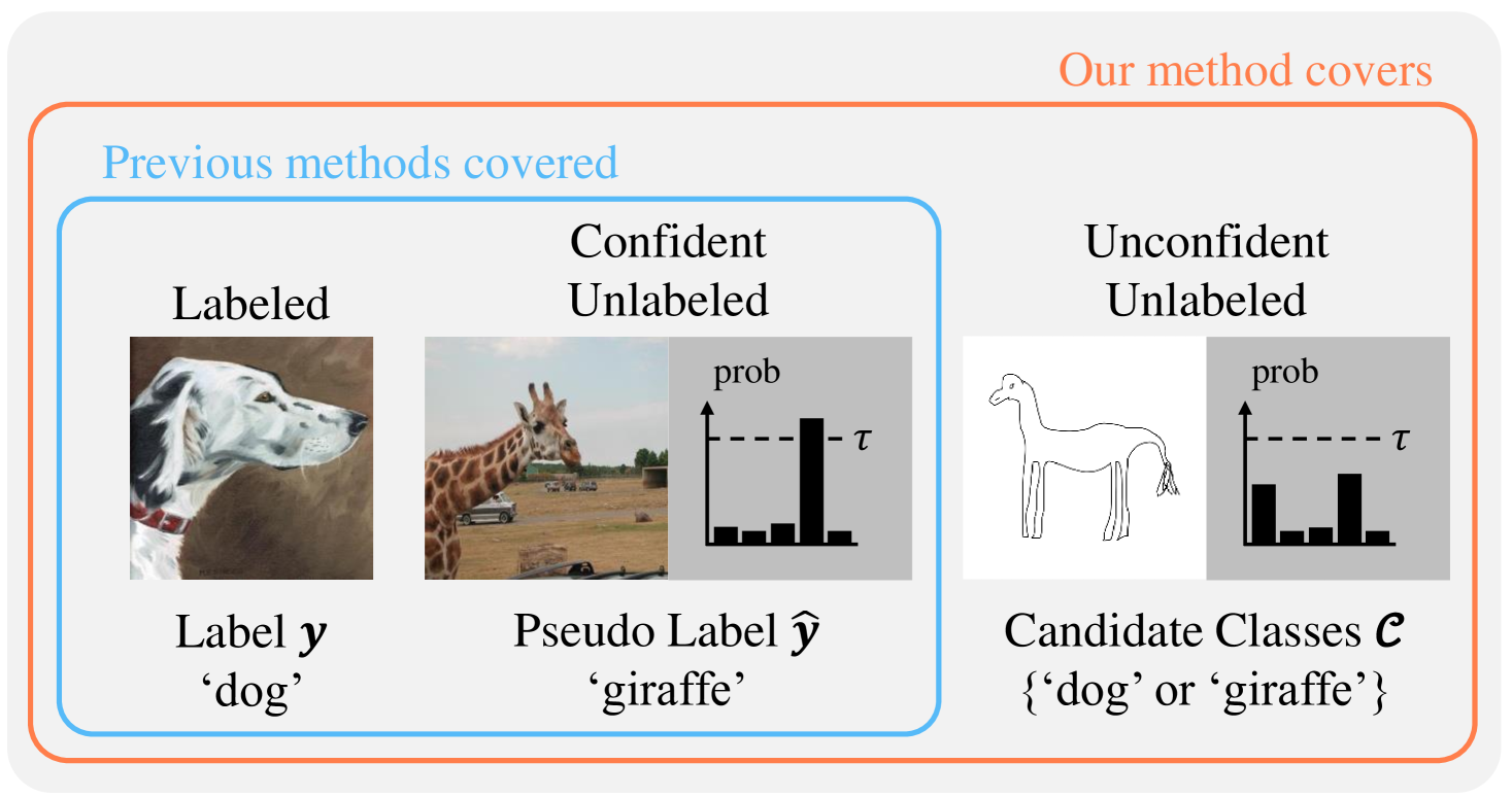
Figure 1: Visual illustration of sample usage differences between previous works and our method in the SSDG task.

Domain generalization (DG) addresses scenarios where the distribution of train data differs from that of test data, a phenomenon known as domain shift. However, it assumes that all train data are fully labeled, which limits data efficiency [19, 17, 31]. For example, in the medical domain, only experts can accurately annotate collected data, making it challenging to obtain a large amount of labeled data due to its labeling cost [16]. Therefore, in such cases, a small amount of labeled data can be used in combination with a large volume of unlabeled data for model training. To address this problem in the presence of domain shift, semi-supervised domain generalization (SSDG) has recently been explored to achieve domain generalizability under sparse labeled scenario [32, 9, 10].

As shown in Fig. 1, existing SSDG methods utilize only confident-unlabeled samples, which model’s prediction is over a certain confidence threshold, restricting the full utilization of the unlabeled data. For example, previous methods employed additional augmentations such as style transfer [32], or utilized domain-wise class prototypes for alignment [9] to create accurate pseudo labels of confident-unlabeled samples. However, these approaches overlook a significant portion of the unlabeled data, whose confidence falls below the confidence threshold, referred to as unconfident-unlabeled samples, as shown in Table 1. This unused data could provide valuable supervisory signals but remains untapped in current methods. This gap motivates us to explore the use of all unlabeled samples in the SSDG, encompassing both confident-unlabeled and unconfident-unlabeled samples. The key question arises: Would incorporating unconfident-unlabeled samples actually impede the learning process, or could it offer untapped benefits?

Table 1: Ratio of unconfident-unlabeled samples relative to the total unlabeled data and the ratio of unconfident-unlabeled samples whose ground truth labels are included in the confusing classes. *UUS Rate indicates the Unconfident-Unlabeled Samples Rate. We trained FixMatch for 3 epochs with ResNet18 backbone. Results are aggregated from four domains tested according to the SSDG protocol, with 10 labels per class.

	PACS	OfficeHome	DigitsDG	miniDomainNet
UUS Rate*	0.22	0.51	0.19	0.50
Inclusion Rate	0.70	0.74	0.73	0.69

To address this question, we conducted a simple observation and uncovered an important insight for leveraging unconfident-unlabeled samples in SSDG: When classifying unconfident-unlabeled samples, the model tends to exhibit confusion among few classes. This characteristic can provide additional supervisory signals, suggesting that these samples are not entirely unreliable but hold meaningful information. Fig. 2 presents a graph illustrating the number of classes the model confuses when predicting the class of unconfident-unlabeled samples. As demonstrated in the figure, across all datasets, the model tends to be confused among typically between 2 to 3 classes for datasets with a small number of classes and mostly up to 15% of classes for datasets with a larger number of classes. Additionally, as summarized in Table 1, we observe that around 70% of the unlabeled-unconfident samples contain its ground truth label in their confusing class set. This also suggests that for each unconfident-unlabeled sample, the ground truth label is likely absent from classes outside this set. Based on this observation, we hypothesize that these samples can provide useful guidance to improve model performance rather than being discarded.

In this paper, we propose UPCSC, a novel method that effectively leverages unconfident-unlabeled samples–data entirely overlooked in previous SSDG methods–based on the observation. To the best of our knowledge, we are the first to utilize unconfident-unlabeled samples in SSDG. To utilize unconfident-unlabeled samples, we propose two contrastive learning-based modules. 1) Unlabeled Proxy-based Contrastive learning (UPC) module: treating unconfident-unlabeled samples as additional negative pairs and 2) Surrogate Class learning (SC) module: generating positive pairs for unconfident-unlabeled samples using their confusing class set. Our method is designed as plug-and-play, making it easily integrated with existing baseline models without requiring substantial modifications to the underlying architecture. we conduct experiments on four widely used SSDG benchmarks to demonstrate that our approach consistently improves performance when attached to baselines and outperforms competing plug-and-play methods. Through extensive analyses, we show that not only does UPCSC enhance class-level discriminability and reduce domain gaps, but it also unlocks the potential of previously unused data, demonstrating the benefits of leveraging all unlabeled samples in SSDG.

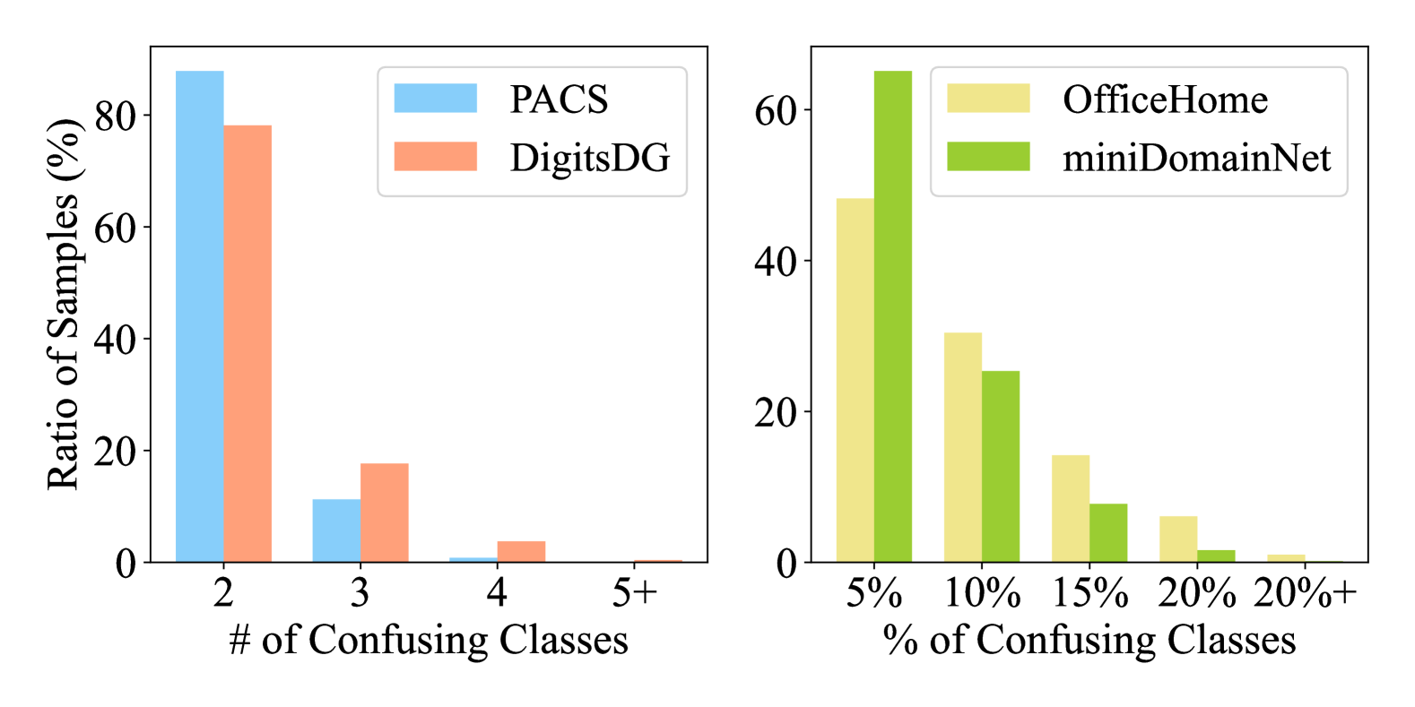
Figure 2: Distribution of the number of classes that unconfident-unlabeled samples are confusing, according to Table 1. We define confusing classes as those of which confidence exceeds the random chance threshold (1/number of classes). Notably, the model tends to confuse samples among only a small subset of classes.

The summary of our contribution is as follows:

• To the best of our knowledge, we introduce the first method to leverage unconfident-unlabeled samples in SSDG.

• We propose UPCSC, a plug-and-play method designed to fully utilize the potential of unlabeled data, demonstrating consistent and significant improvements over the baseline.

• Through extensive analyses, we demonstrate that UPCSC enhances class-level discriminability and mitigates the domain gap.

2 Related Works

2.1 Domain Generalization

Domain generalization (DG) [11, 8, 20, 3] aims to enable models to perform well on unseen domains. One of the promising approaches is to leverage contrastive learning (CL) [5] which is a technique that assigns samples within a batch to different classes and trains the model to be invariant to various augmentations, preventing it from converging on trivial solutions. Numerous studies have leveraged the effectiveness of CL for DG tasks, which aim to help models perform well on unseen domains [15, 27, 17, 21]. In PCL [27], a class-wise proxy vector from classifier weight is assigned as the positive pair for each instance, while samples from different classes within the batch are treated as negative pairs to learn the proxy-to-sample relationship. In this paper, we introduce PCL to the relatively underexplored SSDG setting and demonstrate how it can be utilized in scenarios with unlabeled data.

2.2 Semi-Supervised Learning

Collecting unlabeled data is relatively easier compared to labeled data. Semi-supervised learning (SSL) focuses on how to effectively leverage such unlabeled data alongside a small amount of labeled data during training. One of the most representative SSL works is FixMatch [23], which generates pseudo labels from weakly augmented samples and trains the model to ensure that the predictions on strongly augmented samples align with these pseudo labels. Following the introduction of FixMatch, numerous methods [29, 26, 12, 1] have been proposed to enhance its performance. For example, FlexMatch [29] introduces a curriculum-based pseudo-labeling strategy that adjusts class-wise thresholds according to the model’s learning status. FreeMatch [26] extends the ideas of FlexMatch by introducing self-adaptive global and local thresholds, along with self-adaptive fairness regularization, thereby enabling more unlabeled data to participate in the training process. In this paper, we similarly aim to enable a greater amount of unlabeled data to contribute during the training.

2.3 Semi-Supervised Domain Generalization

Semi-supervised domain generalization (SSDG) aims to perform domain generalization in scenarios where limited labeled data and substantial unlabeled data are available. One of the pioneering studies in the field of SSDG, StyleMatch [32], learned domain-generalized features by combining additional style-augmented samples generated via a style transfer network [14] with FixMatch. Another study, FBCSA [9], addressed the SSDG problem by employing plug-and-play modules called a feature-based conformity module and a semantic alignment module. However, previous studies did not utilize unconfident-unlabeled samples at all during training due to their unreliability. Based on the observation above, this paper proposes a new approach that leverages meaningful information from unconfident-unlabeled samples, achieving a significant contribution that differentiates us from previous studies.

3 Problem

3.1 Problem Formulation

Let us first examine the conventional multi-source DG. Let $\mathcal{X}$ and $\mathcal{Y}$ denote the input and label space, respectively, and let $d$ represent the index of $D$ distinct source domains, where $d\in\{1,\cdots,D\}$. The input $x\sim\mathcal{X}$ and the corresponding label $y\sim\mathcal{Y}$ form a pair, and each sample is represented by their joint distribution $P(\mathcal{X},\mathcal{Y})$. Each domain has distinct characteristics, resulting in a unique distribution $P(\mathcal{X}_{d},\mathcal{Y}_{d})$. Although there may be a shift in $\mathcal{X}_{d}$ for each domain, $\mathcal{Y}_{d}$ is shared consistently across all domains. The data for each domain is denoted by $S_{d}=\{(x_{d},y_{d})\}\sim(\mathcal{X}_{d},\mathcal{Y}_{d})$, and during training, the model has access to $D$ distinct source domains.

SSDG task is a variant of conventional DG, where only a small portion of data remains labeled, and the rest is replaced with unlabeled data. The labeled samples from each domain are defined as $S^{l}_{d}=\{(x^{l}_{d},y^{l}_{d})\}\sim P(\mathcal{X}_{d},\mathcal{Y}_{d})$, while the unlabeled samples from each domain, which only provide access to the input data, are defined as $S^{u}_{d}=\{x^{u}_{d}\}\sim P(\mathcal{X}_{d})$. Due to the cost of labeling, the size of the unlabeled data is generally much larger, i.e. $|S^{u}_{d}|\gg|S^{l}_{d}|$.

The goal of SSDG is to train a domain-agnostic model by effectively utilizing both labeled and unlabeled data from each domain. The model trained on source domains $\{S_{d}\}_{d=1}^{D}$ is evaluated at test time on an unseen target domain $T=\{(x^{*},y^{*})\}\sim P(\mathcal{X}^{*},\mathcal{Y}^{*})$. In this setting, the label spaces of the target and source domains are identical, but the input space of the target domain does not overlap with any source domain, meaning $P(\mathcal{Y}^{*})=P(\mathcal{Y}_{d})$ and $P(\mathcal{X}^{*})\neq P(\mathcal{X}_{d})$ for all $d\in\{1,\cdots,D\}$.

3.2 Limitations and Motivations

Existing studies have addressed SSDG setting by employing data augmentation [32], or domain-specific guidance [9, 10] to assign accurate pseudo label. While these methods have shown a certain level of success, they still leave room for improvement as they do not leverage the information from unconfident-unlabeled samples due to their unreliable prediction. Alternatively stated, existing SSDG approaches assign pseudo labels solely to high-confidence samples, utilizing only these samples for training.

In the early training stages, low-confidence model predictions often lead to poor pseudo label quality, causing a scarcity of pseudo labels. Consequently, pseudo label-based methods heavily rely on limited easy-to-judge data in these early stages, which may be skewed toward a particular class or domain. This, in turn, anchors the model to its initial predictions, hindering its ability to learn domain-generalizable features which is severe for the SSDG task.

We reached the conclusion that the pseudo label-based approach alone has a clear limitation in effectively leveraging unlabeled data in SSDG. Therefore, we explored a new method that can also utilize unconfident-unlabeled samples without assigning pseudo labels. Notably, we observed that these unconfident-unlabeled samples are mostly confused among a small subset of classes (Fig. 2), which we call candidate classes. Based on this, we used the remaining excluded classes, which are likely not the correct class, as additional negative pairs by unlabeled proxy-based contrastive learning (Sec. 4.1). Furthermore, to incorporate the information from the candidate classes into training, we introduce a surrogate class, obtained as a weighted sum of class proxies, and used it as a positive pair for unconfident-unlabeled samples (Sec. 4.2).

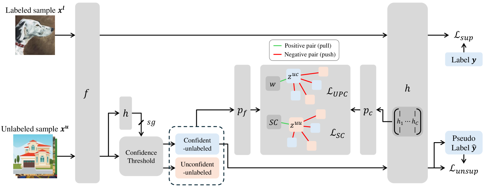
Figure 3: Overview of our UPCSC algorithm. UPCSC is a plug-and-play module designed to be implemented atop SSL-based SSDG methods. To fully leverage unlabeled data in the SSDG setting, we propose two novel learning methods: Unlabeld Proxy-based Contrast learning (UPC) and Surrogate Class learning (SC).

4 Method

We introduce UPCSC, a plug-and-play method that enables the additional use of information from unconfident-unlabeled samples by simply adding them onto existing SSL-based baseline. Our UPCSC incorporates all unlabeled samples encompassing both confident- and unconfident-unlabeled samples, through a contrastive learning-based approach. Inspired by proxy-based contrastive learning [27], features and class proxies in the contrastive learning process pass through their respective 1-layer MLP projectors. Figure 3 visualizes the overall architecture of our method.

Notations We further denote the featurizer and classifier from the existing SSL-based baselines as $f$ and $h$, respectively, where the classifier weights consist of class proxies $h=[h_{1},h_{2},\ldots,h_{C}]$ and C is the number of classes. The featurizer maps an arbitrary input $x$ to a feature, which is then passed through the classifier and softmax function, yielding class confidences $c(x)=\text{softmax}((h\circ f)(x))\in\mathbb{R}^{C}$. For unlabeled data $x^{u}$, the pseudo label is assigned as $\hat{y}=\text{argmax}(c(x^{u}))$ if $\max(c(x^{u}))\geq\tau$, where $\tau$ is a confidence threshold. Note that, pseudo labels are defined only for samples with max confidence exceeding $\tau$.

In proxy-based contrastive learning, normalized embeddings after passing through a projector are used. Two projectors attached to featurizer and classifier are referred to as the feature projector $p_{f}$ and classifier projector $p_{c}$, respectively. Thus, the newly embedded feature $z_{i}$ and proxy $w_{i}$ are denoted as $z_{i}=\|p_{f}(f(x_{i}))\|$ and $w_{i}=\|p_{c}(h_{i})\|$, respectively, where $\|\cdot\|$ denotes the normalization operation. PCL and our method share the notation.

We also define an unlabeled sample of which max confidence $\max(c(x^{u}))$ exceeding $\tau$ as a confident-unlabeled sample $x^{uc}$, while an unlabeled sample of which max confidence below $\tau$ as unconfident-unlabeled sample $x^{uu}$. When the $i$-th unconfident-unlabeled sample $x^{uu}_{i}$ is uncertain among few classes, we refer this classes as sample’s candidate class set $\mathcal{C}_{i}=\{y|[c(x^{uu}_{i})]_{y}>1/C\}$, while its excluded class set is defined as $\mathcal{E}_{i}=\mathcal{Y}\setminus\mathcal{C}_{i}$. The terms are visually illustrated in Fig. 4. Unlike other SSDG methods, we do not utilize domain labels during training; thus, for simplicity, the source domain index, $d$, is omitted below.

4.1 Unlabeled Proxy-based Contrastive Learning

We introduce the Unlabeled Proxy-based Contrastive learning (UPC) module, which applies supervised contrastive learning to confident-unlabeled samples while leveraging unconfident-unlabeled samples as additional negative pairs. For confident-unlabeled samples, following previous studies [23, 32], we assign pseudo labels and treat them as labeled samples. However, because unconfident-unlabeled samples lack reliable predictions, they cannot be used in the same way and require a novel approach.

The outline of UPC is as follows: for a confident-unlabeled sample $x^{uc}\in\{x|\max(c(x))\geq\tau,~\hat{y}(x)=y^{\prime}\}$ with max confidence $\max(c(x))$ exceeding a threshold $\tau$ and pseudo label $\hat{y}(x)=y^{\prime}$, the positive pair is the class proxy $w_{y^{\prime}}$ corresponding to its pseudo label $y^{\prime}$. The negative pairs include confident-unlabeled samples $\mathcal{X}^{uc}_{upc}=\{x|\max(c(x))\geq\tau,~\hat{y}(x)\neq y^{\prime}\}$ with pseudo labels $\hat{y}(x)\neq y^{\prime}$, as well as unconfident-unlabeled samples $\mathcal{X}^{uu}_{upc}=\{x|\max(c(x))<\tau,~y^{\prime}\in\mathcal{E}(x)\}$, for which $y^{\prime}$ is an element of the excluded class set.

Contrastive-based loss has the advantage of directly reflecting the relationship between samples, making it well-suited for our approach that utilizes a larger number of samples due to the inclusion of unconfident-unlabeled samples. Eq. 1 represents the proxy-based contrastive learning (PCL) loss in a scenario where all samples are labeled. It minimizes the loss by maximizing the inner product between the feature $z_{i}$ of the target sample $x_{i}$ and the corresponding class proxy $w_{y_{i}}$ while minimizing the inner product with features from negative pairs of other classes within a mini-batch of N samples:

$$\small\mathcal{L}_{PCL}=-\frac{1}{N}\sum_{i=1}^{N}\log{\frac{\exp(z_{i}\cdot w_{y_{i}})}{\exp(z_{i}\cdot w_{y_{i}})+\sum_{\{j|y_{j}\neq y_{i}\}}{\exp(z_{i}\cdot z_{j})}}}.$$ (1)

We apply this approach to handle unlabeled samples by providing a loss for the confident-unlabeled samples. Eq. 2 defines the UPC loss, extending Eq. 1, by additionally incorporating unconfident-unlabeled samples features $z^{uu}$ as extra negative pairs. Samples selected based on the criteria described above are used here:

$$\mathcal{L}_{UPC}=-\frac{1}{N^{uc}}\displaystyle\sum_{i=1}^{N^{uc}}\log{\frac{\exp(z^{uc}_{i}\cdot w_{\hat{y}_{i}})}{\exp(z^{uc}_{i}\cdot w_{\hat{y}_{i}})+R}}~~\text{where}\\ R=\displaystyle\sum_{\{j|\hat{y}_{j}\neq\hat{y}_{i}\}}{\exp(z^{uc}_{i}\cdot z^{uc}_{j})}+\displaystyle\sum_{\{j|\hat{y}_{i}\in\mathcal{E}_{j}\}}{\exp(z^{uc}_{i}\cdot z^{uu}_{j})}.$$ (2)

Here, $N^{uc}$ represents the number of unconfident-unlabeled samples in a mini-batch.

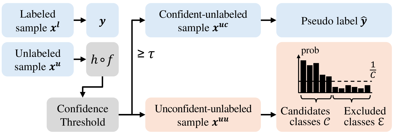
Figure 4: High level idea of our method and terminology

Table 2: The results show the SSDG accuracy(%) in a 10 labels per class setting across various benchmarks. The results report the average over five different random seeds. The numbers in parentheses represent the change compared to the baseline model.

Model PACS OH DigitsDG DN ERM [6] 60.2 $\pm$ 2.0 54.2 $\pm$ 0.5 60.8 $\pm$ 3.1 48.8 $\pm$ 0.2 MeanTeacher [24] 66.0 $\pm$ 2.6 56.7 $\pm$ 0.3 63.3 $\pm$ 2.6 49.4 $\pm$ 0.2 FreeMatch [26] 73.5 $\pm$ 1.1 57.7 $\pm$ 0.4 74.2 $\pm$ 2.1 54.8 $\pm$ 0.2 FixMatch [23] 76.8 $\pm$ 1.1 57.7 $\pm$ 0.4 75.1 $\pm$ 1.1 54.5 $\pm$ 0.3 StyleMatch [32] 79.9 $\pm$ 1.0 59.7 $\pm$ 0.3 78.4 $\pm$ 0.4 55.0 $\pm$ 0.2 FreeMatch + Ours 77.8 $\pm$ 1.4 (+4.3) 59.1 $\pm$ 0.5 (+1.4) 80.4 $\pm$ 0.7 (+6.2) 56.5 $\pm$ 0.3 (+1.7) FixMatch + Ours 79.6 $\pm$ 0.7 (+2.9) 58.6 $\pm$ 0.2 (+0.9) 80.7 $\pm$ 1.1 (+5.6) 56.0 $\pm$ 0.3 (+1.5) StyleMatch + Ours 81.5 $\pm$ 0.8 (+1.6) 59.9 $\pm$ 0.2 (+0.2) 82.2 $\pm$ 0.6 (+3.8) 55.6 $\pm$ 0.3 (+0.6)

Table 3: The results show the SSDG accuracy(%) in a 5 labels per class setting across various benchmarks. The results report the average over five different random seeds. The numbers in parentheses represent the change compared to the baseline model.

Model PACS OH DigitsDG DN ERM [6] 55.2 $\pm$ 2.5 52.2 $\pm$ 0.6 42.6 $\pm$ 2.7 44.4 $\pm$ 0.3 MeanTeacher [24] 60.6 $\pm$ 1.8 52.7 $\pm$ 0.9 45.4 $\pm$ 2.4 44.4 $\pm$ 0.4 FreeMatch [26] 71.6 $\pm$ 1.8 55.9 $\pm$ 0.5 63.3 $\pm$ 2.8 52.0 $\pm$ 0.7 FixMatch [23] 73.6 $\pm$ 2.9 55.0 $\pm$ 0.6 64.7 $\pm$ 3.8 51.6 $\pm$ 0.3 StyleMatch [32] 78.9 $\pm$ 0.8 56.5 $\pm$ 0.5 71.9 $\pm$ 2.9 51.0 $\pm$ 0.4 FreeMatch + Ours 73.5 $\pm$ 2.1 (+1.9) 56.8 $\pm$ 0.8 (+0.9) 76.4 $\pm$ 0.6 (+13.1) 53.7 $\pm$ 0.4 (+1.7) FixMatch + Ours 78.9 $\pm$ 0.9 (+5.3) 56.1 $\pm$ 0.6 (+1.1) 75.2 $\pm$ 2.6 (+10.5) 52.7 $\pm$ 0.4 (+1.1) StyleMatch + Ours 79.8 $\pm$ 3.2 (+0.5) 56.8 $\pm$ 0.8 (+0.3) 76.7 $\pm$ 2.1 (+4.8) 51.2 $\pm$ 0.2 (+0.2)

4.2 Surrogate Class Learning

Next, we introduce the Surrogate Class (SC) module, which generates positive pairs for unconfident-unlabeled samples by utilizing their candidate classes–a set of potential labels–to enable contrastive learning. The SC proxy, created as a confidence-weighted sum of candidate class proxies, serves as a positive pair in contrastive learning for unconfident-unlabeled samples that cannot be assigned a specific label, acting as a surrogate for a particular class proxy. This SC proxy is computed individually for each sample and is recalculated in every iteration since the confidence value of each sample changes as the model is updated.

The aim of SC module is to provide appropriate guidance for unconfident-unlabeled samples that are uncertain about their true labels, thereby increasing confidence towards the correct class and ultimately assigning the correct pseudo label. Previous work [4] demonstrated the effectiveness of simultaneously assigning two class labels to uncertain unlabeled samples. We extend this approach to adaptively handle two or more classes, thereby enabling our method to accommodate cases with a large number of candidate classes.

Eq. 3 defines the formula for obtaining the SC proxy for a given sample $x^{uu}$. The proxies of candidate classes whose confidence exceeds the random guessing threshold $1/C$, are selectively aggregated. These proxies are weighted by the class confidence $c(x)=[c(x)_{1},c(x)_{2},\ldots,c(x)_{C}]$ for each class:

$$SC(x^{uu})=\sum_{i=1}^{C}\mathbbm{1}([c(x^{uu})]_{i}>1/C)\cdot[c(x^{uu})]_{i}\cdot w_{i},$$ (3)

where $\mathbbm{1}$ is the indicator function.

The outline of SC is as follows: Consider an unconfident-unlabeled samples $x^{uu}\in\{x|max(c(x))<\tau\}$, where its candidate class set and excluded class set are denoted as $\mathcal{C}^{\prime}$ and $\mathcal{E}^{\prime}$, respectively. The positive pair is the corresponding surrogate class $SC(x^{uu})$, while negative pairs include confident-unlabeled samples $\mathcal{X}^{uc}_{sc}=\{x|max(c(x))\geq\tau,~\hat{y}(x)\in\mathcal{E}^{\prime}\}$ with a pseudo label $\hat{y}$ belonging to the excluded class set, as well as unconfident-unlabeled samples $\mathcal{X}^{uu}_{sc}=\{x|max(c(x))<\tau,~\mathcal{C}(x)\cap\mathcal{C}^{\prime}=\emptyset\}$ of which candidate classes have no overlapping elements.

Eq. 4 defines the contrastive-based SC loss, which is computed using these selected positive and negative pairs:

$$\mathcal{L}_{SC}=-\frac{1}{N^{uu}}\sum_{i=1}^{N^{uu}}\log\frac{\exp(z^{uu}_{i}\cdot SC(x^{uu}_{i}))}{\exp(z^{uu}_{i}\cdot SC(x^{uu}_{i}))+R}~~\text{where}\\ R=\displaystyle\sum_{\{j|\hat{y}_{j}\in\mathcal{E}_{i}\}}{\exp(z^{uu}_{i}\cdot z^{uc}_{j})}+\displaystyle\sum_{\{j|\mathcal{C}_{j}\cap\mathcal{C}_{i}=\emptyset\}}{\exp(z^{uu}_{i}\cdot z^{uu}_{j})}.$$ (4)

Here, $N^{uu}$ represents the number of unconfident-unlabeled samples in a mini-batch.

Our method also seamlessly integrates with data augmentation used in SSL-based baselines. The contrastive learning architecture, consisting of both UPC and SC modules, utilizes all augmented samples generated by the baseline algorithm as contrastive elements. For instance, StyleMatch, which uses three types of augmentations, the modules utilize a total of $3\times N$ samples. This effectively increases the number of available samples, enabling more information-abundant contrastive learning.

4.3 Total Objective for Training

UPCSC is a plug-and-play method that can be utilized alongside existing SSL-based baselines. Previous SSL-based approaches comprise a supervised loss ($\mathcal{L}_{\text{sup}}$) and an unsupervised consistency loss ($\mathcal{L}_{\text{unsup}}$). The supervised loss, $\mathcal{L}_{\text{sup}}$, applies a standard cross-entropy (CE) loss on labeled data. In contrast, $\mathcal{L}_{\text{unsup}}$ generates pseudo labels by using model predictions from weakly augmented samples of confident-unlabeled samples and applies a CE loss to encourage the model prediction of strongly augmented samples to align with these pseudo labels. Based on this, the objective for training the model with the UPCSC method plugging on top of the baseline method is as follows:

$$\mathcal{L}_{\text{total}}=\mathcal{L}_{\text{sup}}+\mathcal{L}_{\text{unsup}}+\mathcal{L}_{\text{UPC}}+\mathcal{L}_{\text{SC}}.$$ (5)

5 Experiments

Table 4: Comparison of various plug-and-play methods in SSDG under 10 labels and 5 labels per class settings. Each result represents the average over five different random seeds.

Model	Labels per class = 10				Labels per class = 5
	PACS	OH	DigitsDG	DN	PACS	OH	DigitsDG	DN
FixMatch [23]	76.8 $\pm$ 1.1	57.7 $\pm$ 0.4	75.1 $\pm$ 1.1	54.5 $\pm$ 0.3	73.6 $\pm$ 3.0	55.0 $\pm$ 0.6	64.7 $\pm$ 3.8	51.6 $\pm$ 0.3
FixMatch + FBCSA [9]	77.7 $\pm$ 1.6	58.7 $\pm$ 0.4	80.5 $\pm$ 1.3	55.6 $\pm$ 0.3	74.2 $\pm$ 2.9	55.6 $\pm$ 0.4	75.5 $\pm$ 0.9	50.1 $\pm$ 0.2
FixMatch + DGWM [10]	78.8 $\pm$ 0.9	59.4 $\pm$ 0.4	75.5 $\pm$ 1.7	53.7 $\pm$ 0.5	78.0 $\pm$ 1.3	56.1 $\pm$ 0.4	67.9 $\pm$ 3.2	50.3 $\pm$ 0.7
FixMatch + Ours	79.6 $\pm$ 0.7	58.6 $\pm$ 0.2	80.7 $\pm$ 1.1	56.0 $\pm$ 0.3	78.9 $\pm$ 0.9	56.1 $\pm$ 0.6	75.2 $\pm$ 2.6	52.7 $\pm$ 0.4
StyleMatch [32]	79.9 $\pm$ 0.9	59.7 $\pm$ 0.3	78.4 $\pm$ 0.5	55.0 $\pm$ 0.2	78.9 $\pm$ 0.8	56.5 $\pm$ 0.5	71.9 $\pm$ 2.9	51.0 $\pm$ 0.4
StyleMatch + FBCSA [9]	79.3 $\pm$ 3.0	60.0 $\pm$ 0.3	80.5 $\pm$ 1.4	55.0 $\pm$ 0.3	76.8 $\pm$ 2.6	55.8 $\pm$ 0.3	75.8 $\pm$ 5.7	50.1 $\pm$ 0.2
StyleMatch + DGWM [10]	80.4 $\pm$ 1.1	59.7 $\pm$ 0.2	78.3 $\pm$ 1.1	55.0 $\pm$ 0.3	78.9 $\pm$ 1.0	56.3 $\pm$ 0.5	71.9 $\pm$ 1.6	50.8 $\pm$ 0.4
StyleMatch + Ours	81.5 $\pm$ 1.2	59.9 $\pm$ 0.1	82.2 $\pm$ 0.6	55.6 $\pm$ 0.3	79.8 $\pm$ 3.2	56.8 $\pm$ 0.8	76.7 $\pm$ 2.1	51.2 $\pm$ 0.2

5.1 Implementation Details

To evaluate our method, we utilized four widely-used DG datasets: PACS [18], OfficeHome (OH) [25], DigitsDG [30], and miniDomainNet (DN) [22] for SSDG benchmarks. Experiments were conducted under two labeling scenarios: 10 labels and 5 labels per class setting. For each batch, 16 labeled and 16 unlabeled samples were randomly selected from each domain. We adopted an ImageNet [7] pretrained ResNet18 [13] as the backbone and employed a single-layer MLP as the classifier. For a fair comparison among methods, we used the SGD optimizer with a learning rate of 0.003 for the backbone and 0.01 for the classifier, applying cosine learning rate decay to both. Two projectors—the feature projector and classifier projector—are single-layer MLPs with a learning rate of 0.0005, preserving the dimension from the backbone, which is 512 for ResNet18 [13]. For the confidence threshold $\tau$, we followed the settings of each underlying SSL-based baseline. Models are trained for 20 epochs and results are reported as the average top-1 accuracy across five random seeds for all datasets.

For comparison, we selected ERM [6] as a representative DG method, and from SSL approaches, we chose MeanTeacher [24], FreeMatch [26], and FixMatch [23]. For SSDG methods, we included StyleMatch [32], and as plug-and-play baselines, we compared against FBCSA [9] and DGWM [10].

Table 5: Ablation study on PACS and OH under 10 labels per class setting for each component. The results report the average over five different random seeds.

Method	PACS	OH
Fixmatch	76.8	57.7
Fixmatch + UPC	79.2 (+2.4)	58.4 (+0.7)
Fixmatch + SC	77.0 (+0.2)	58.4 (+0.7)
Fixmatch + UPC + SC	79.6 (+2.8)	58.6 (+0.9)

5.2 Results

Table 2 and 3 present the performance across various SSDG benchmarks under the 10 labels and 5 labels per class settings, respectively. As shown in the tables, our method consistently outperforms SSL-based baselines across all benchmarks in a plug-and-play manner without requiring any modifications to existing methodologies. This demonstrates that our approach efficiently leverages all unlabeled data provided during training, effectively addressing both domain shift and SSL problems simultaneously.

Additionally, Table 4 compares our approach with other plug-and-play methods. As shown in the table, our method outperforms the other approaches across most datasets. This demonstrates that leveraging not only confident-unlabeled samples but also unconfident-unlabeled samples brings positive effect in SSDG.

5.3 Ablation study

To further verify the performance contribution of our proposed modules, we conduct an ablation study on each module. Table 5 presents the average accuracy over five random seeds in the PACS and OH 10 labels per class setting, illustrating the performance contribution of each module. As shown in the table, for PACS / OH respectively, applying UPC improved the baseline by 2.4%p / 0.7%p (second row). Incorporating SC increased the improvement to 0.2%p / 0.7%p (third row). Finally, combining UPC and SC led to an enhancement of 2.8%p / 0.9%p (fourth row). These findings suggest that UPC and SC significantly help boost SSDG performance.

5.4 Analysis

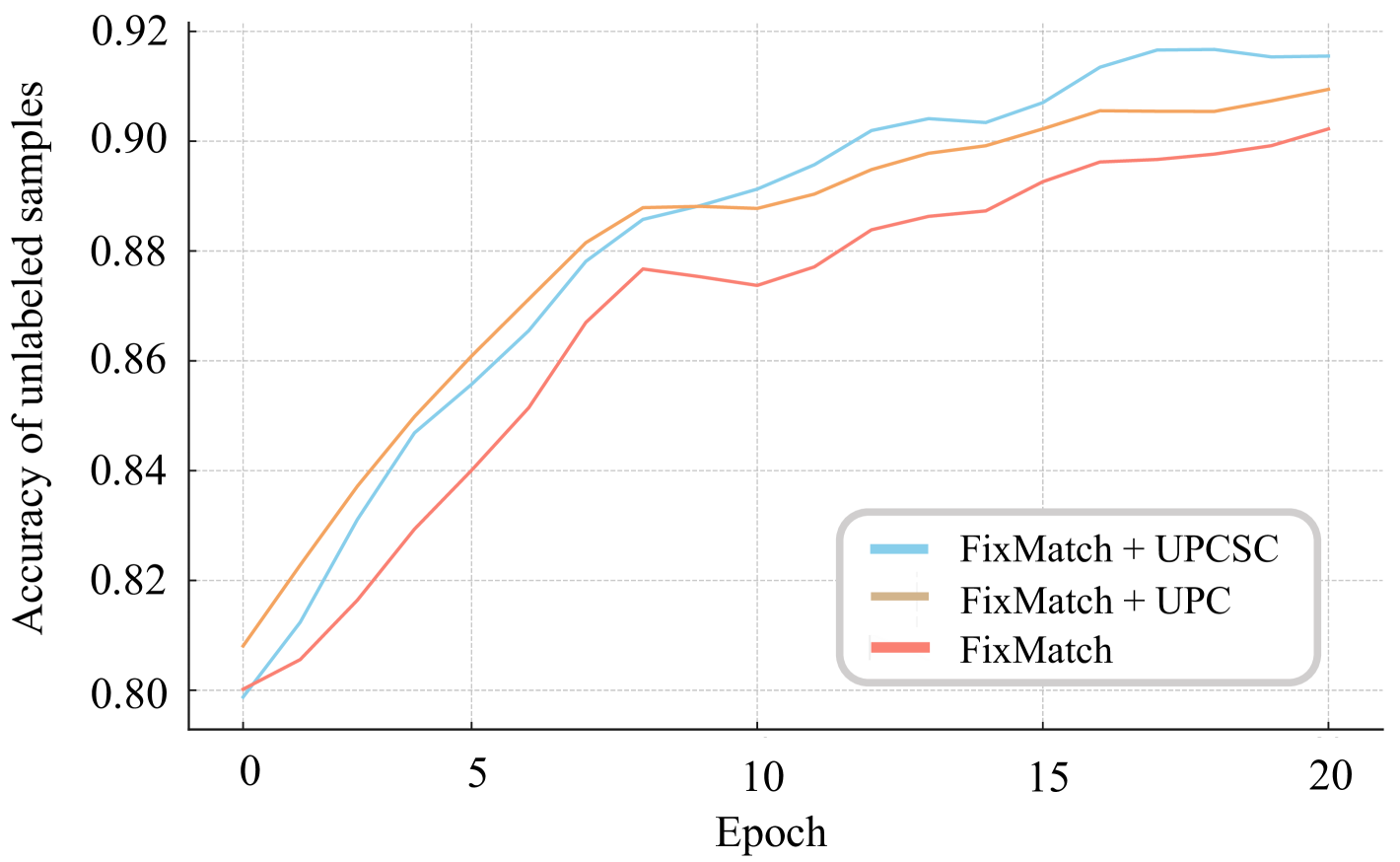
Figure 5: Average accuracy of unlabeled samples from the source domain in the PACS 10 labels per class setting. Note that we do not use any test target domain dataset for calculating accuracy.

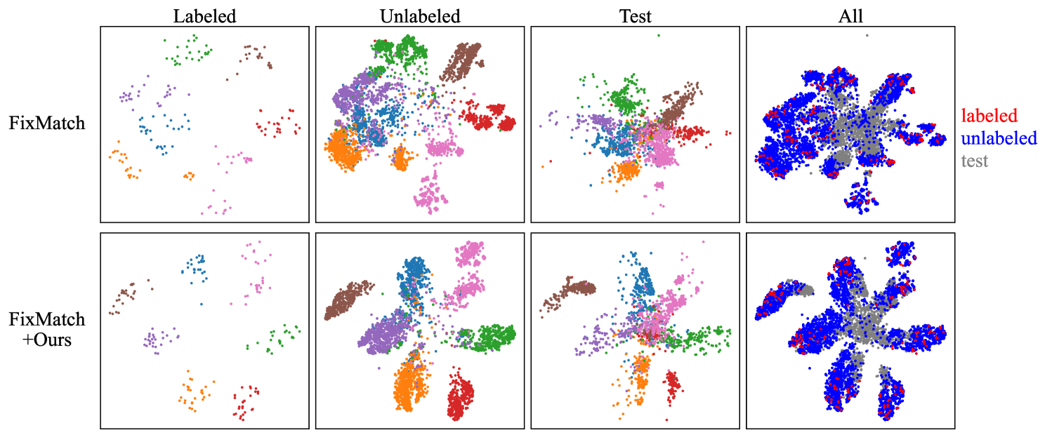
Figure 6: T-SNE visualization of FixMatch and FixMatch + Ours in the PACS 10 labels per class setting. To verify clear class separation, we visualized the labeled source domain dataset (first column), unlabeled source domain dataset (second column), and target domain dataset (third column). In the fourth column, we visualized all source and target domain data together to illustrate effective class-wise clustering even in the presence of domain shift. In this column, labeled source domain data, unlabeled source domain data, and target domain data are shown in red, blue, and gray, respectively.

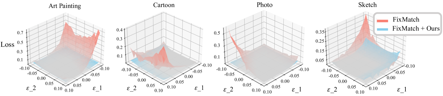
Figure 7: Visualization of the loss landscape of FixMatch and FixMatch + Ours trained under PACS 10 labels per class setting. $\epsilon_{1}$ and $\epsilon_{2}$ denote the first and second eigenvector direction, respectively. The loss landscape is derived using data from the source domain rather than the target domain.

Accuracy of unlabeled train data To examine whether UPCSC effectively utilizes the unlabeled data from the source domain during training, we plotted the average accuracy on all unlabeled source domain data across epochs. As shown in Figure 5, UPC achieves higher accuracy on the unlabeled data from source domain compared to FixMatch. Furthermore, applying SC on top of UPC helps the model to accurately utilize unlabeled source domain data. This demonstrates that by effectively leveraging unconfident-unlabeled samples—previously disregarded in existing methods—UPCSC further brings benefit to the learning process.

Feature visualization To visually analyze the role of UPCSC in the feature space, we present a t-SNE in Figure 6. For this visualization, we used models trained on the PACS 10 labels per class setting, specifically FixMatch and FixMatch + Ours. As seen in the figure, our method enhances class-level discriminability in the source domain (first and second columns). Furthermore, our approach demonstrates stronger class separation even in the unseen test domain compared to FixMatch (third column). Additionally, our method enables domain-agnostic clustering of classes even under the existence of severe domain shift (fourth column). These findings underscore that our method effectively enhances class-level discriminability and reduces domain gaps in a plug-and-play manner.

Loss Landscape To demonstrate that our method effectively reduces domain gap, we visualized the loss landscape, building on SWAD’s [2] argument that optimizing for flat minima reduces domain gaps. As shown in Figure 7, our method converges to flatter minima compared to FixMatch, underscoring its potential to reduce domain gaps effectively as a plug-and-play approach. Specifically, we employed PyHessian [28] for loss landscape visualization, perturbing the model parameters along the directions of the first and second Hessian eigenvectors to compare the loss landscapes of our method and the baseline, FixMatch. This visualization was conducted using the source domain dataset in the PACS 10 labels per class setting.

6 Conclusion

In this paper, we introduce our novel method UPCSC to address SSDG, closely aligned with real-world scenarios. Our method consists of two modules, an Unlabeled Proxy-based Contrastive learning (UPC) module and a Surrogate Class learning (SC) module, which leverage the full potential of unlabeled data in SSDG. To validate the effectiveness of our method, we conducted experiments on various benchmarks used in SSDG, demonstrating consistent performance improvements by applying our methods in a plug-and-play manner to SSL-based baseline methods. Through extensive analyses, we show that our method enhances class-level discriminability and mitigates domain gap.

Supplementary Material

A Dataset Description

We conduct experiments on four SSDG benchmarks. The PACS dataset comprises four domains: art-painting, cartoon, photo, and sketch, and includes seven classes: dog, elephant, giraffe, guitar, horse, house, and person. The OfficeHome dataset consists of four domains: art, clipart, product, and real-world, with a total of 65 classes. The miniDomainNet dataset includes four domains: clipart, painting, real, and sketch, and contains 345 classes. Lastly, the DigitsDG dataset is composed of four domains: MNIST, MNIST-M, SVHN, and SYN, and features 10 classes, ranging from 0 to 9.

B Psuedo Code Algorithm

To illustrate the detailed implementation of the UPCSC method, we provide a pseudo code in Algorithm A. For simplicity, the domain label index $d$, weak augmentation $\alpha$, and strong augmentation $\mathcal{A}$ are omitted.

C Loss for SSL-based baseline

In this section, we give a detailed description on loss for SSL-based baselines, such as FixMatch. SSL-based baselines comprise a supervised loss ($L_{sup}$) using labeled data $x^{l}$, and an unsupervised consistency loss ($L_{unsup}$) which leverages confident-unlabeled samples $x^{uc}$. $L_{sup}$ is computed for labeled data as follows:

$$L_{sup}=\text{CE}(\text{softmax}((h\circ f)(x^{l})),y^{l}).$$ (6)

The unsupervised consistency loss, $L_{unsup}$, utilizes confident-unlabeled samples $x^{uc}$ with pseudo-labels $\hat{y}=\text{argmax}(\text{softmax}((h\circ f)(\alpha(x^{uc}))))$ generated via weak augmentation $\alpha$. This loss ensures that the predictions for strongly augmented samples $\mathcal{A}(x^{uc})$ are aligned with their pseudo-labels. Formally, the unsupervised consistency loss is computed as follows:

$$L_{unsup}=\text{CE}(\text{softmax}((h\circ f)(\mathcal{A}(x^{uc}))),\hat{y}).$$ (7)

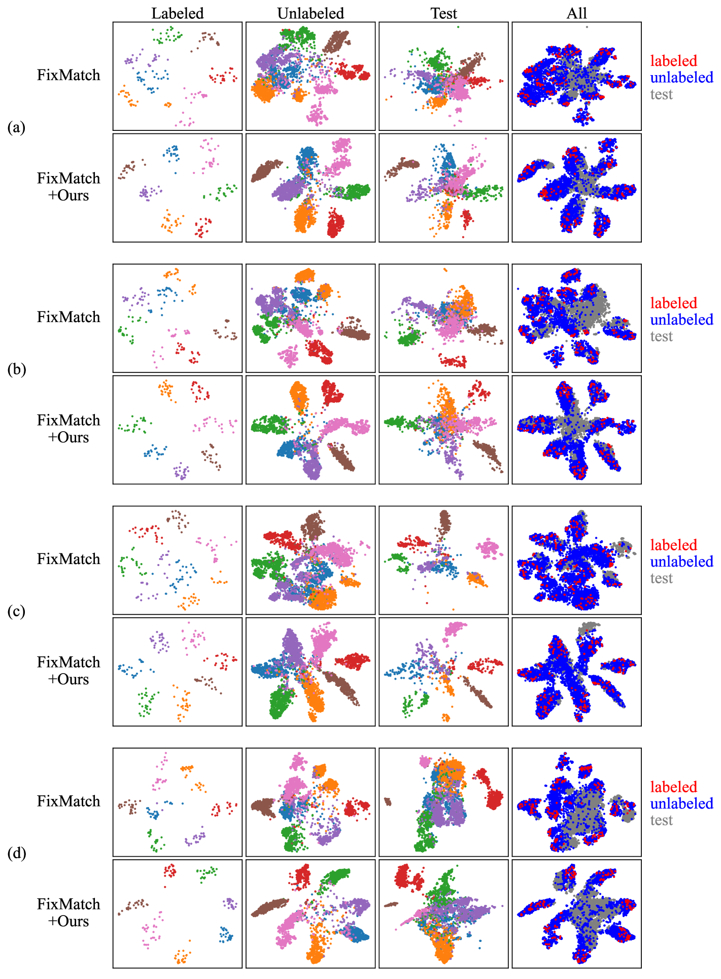
Figure A: T-SNE visualization of FixMatch and FixMatch + Ours in the PACS dataset under the 10 labels per class setting are presented for each domain. Each sub-figure corresponds to the target domain being (a) art-painting, (b) cartoon, (c) photo, and (d) sketch, respectively.

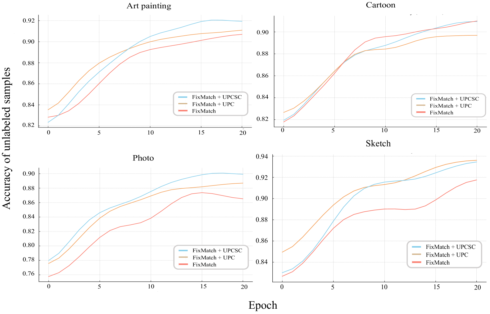
Figure B: Accuracy of unlabeled samples from the source domain in the PACS 10 labels per class setting for each domain.

D T-SNE Visualization by Domain

In Fig. A, we provide the visualizations of t-SNE for each domain, a more specific version of t-SNE represented in the analysis section, Fig. 6. To explain further the visualization procedure, the t-SNE visualization for a specific domain is performed on a model trained with that domain as the target domain. Since the model is not accessible to the target domain data during training, the labeled and unlabeled train data (source data) are drawn from the remaining domains, excluding the target domain. The data corresponding to the target domain can only be found in the test data.

E Detailed Visualization on Accuracy of unlabeled train data

In Fig. B, we provide the plot on the accuracy of unlabeled train data for each domain rather than the average which was represented at Fig. 5.

F More Ablation Studies on our proposed modules

Table A summarizes the contributions of our proposed modules to overall performance in various settings. These results demonstrate that the proposed UPC and SC modules substantially boost performance.

Table A: Ablation study of how the proposed UPC and SC modules contribute to performance across various experimental settings.

	PACS		OH
Labels per class	10	5	10	5
FixMatch	76.8	73.6	57.7	55.0
+UPC	79.2	76.8	58.4	55.9
+SC	77.0	77.8	58.4	55.5
+UPCSC	79.6	78.9	58.6	56.1

G Ablation study on UPC

Table B illustrates the importance of incorporating unconfident-unlabeled samples $x^{uu}$ within the UPC module. As shown in the table, excluding these samples yields a 1.2%p improvement over the baseline, while their inclusion raises the margin to 2.4%p. This result clearly demonstrates the benefit of leveraging such unconfident-unlabeled samples for performance enhancement.

Table B: Ablation study on UPC without unconfident-unlabeled samples $x^{uu}$ on PACS 10 labels per class setting. Each result represents the average accuracy.

Method	Accuracy (%)
FixMatch	76.8
+UPC (w/o $x^{uu}$)	78.0
+UPC	79.2
+UPCSC	79.6

H Variants of SC module

Table C presents an ablation study on strategies for generating positive pairs from unconfident-unlabeled samples in the SC module. Here, Top-1 denotes the results obtained by using only the proxy of the highest-confidence class, while Avg. Proxy represents those obtained by averaging all candidate class proxies. Finally, Ours is based on a weighted average of the candidate class proxies.

Table C: Comparison of different positive pair selection strategies for SC in PACS 10 labels per class setting.

Method	Top-1 Proxy	Avg. Proxy	Ours
FixMatch	78.9	80.5	79.6
StyleMatch	78.3	80.2	81.5

Table D: Comparison of various plug-and-play methods incorporated on FreeMatch [26] in SSDG under 10 labels and 5 labels per class settings. Each result represents the average over five different random seeds.

Model	Labels per class = 10				Labels per class = 5
	PACS	OH	DigitsDG	DN	PACS	OH	DigitsDG	DN
FreeMatch [26]	73.5 $\pm$ 1.1	57.7 $\pm$ 0.4	74.2 $\pm$ 2.1	54.8 $\pm$ 0.2	71.6 $\pm$ 1.8	55.9 $\pm$ 0.5	63.3 $\pm$ 2.0	52.0 $\pm$ 0.7
FreeMatch + FBCSA [9]	73.7 $\pm$ 2.3	58.6 $\pm$ 0.4	78.7 $\pm$ 0.9	55.5 $\pm$ 0.3	69.2 $\pm$ 1.4	55.8 $\pm$ 0.3	76.2 $\pm$ 1.0	51.0 $\pm$ 0.7
FreeMatch + DGWM [10]	73.3 $\pm$ 1.3	57.6 $\pm$ 0.4	74.0 $\pm$ 0.7	54.7 $\pm$ 0.3	72.2 $\pm$ 1.9	55.8 $\pm$ 0.6	62.2 $\pm$ 4.3	52.0 $\pm$ 0.5
FreeMatch + Ours	77.8 $\pm$ 1.4	59.1 $\pm$ 0.5	80.4 $\pm$ 0.7	56.5 $\pm$ 0.3	73.5 $\pm$ 2.1	56.8 $\pm$ 0.8	76.4 $\pm$ 0.6	53.7 $\pm$ 0.4

I Additional Experiment Results

Table D shows the results of applying the plug-and-play methods to FreeMatch as a complement to Table 4, which presents the results of applying these plug-and-play methods to FixMatch and StyleMatch. Notably, when applied to FreeMatch, our method demonstrates superior performance compared to other plug-and-play approaches across all datasets. Due to space constraints in the main text, the results for FreeMatch are included in the supplementary material.

J Code Asset

In Sec. 5.2, we used the benchmark introduced in StyleMatch [32]. The code of this work is also built upon this work. Authors thank to their open sourcing.

Algorithm A Pseudo Code of UPCSC

0:  Labeled data $(x^{l},y^{l})$, unlabeled data $(x^{u})$, confidence threshold $\tau$, number of classes $C$, total epochs $E$, feature projector $p_{f}$, classifier projector $p_{c}$, featurizer $f$, classifier $h=[h_{1},h_{2},\ldots,h_{C}]$, normalization operation $\lVert\cdot\rVert$, indexing operation $[\cdot]_{i}$ for selecting $i$-th element.

1:  for epoch = 1 to E do

2:   Step 1: Divide Confident-Unlabeled and Unconfident-Unlabeled Samples

3:   $c(x)=\text{softmax}((h\circ f)(x))$

4:   $x^{uc}=\{x\mid\max(c(x))\geq\tau,\text{ }x\in x^{u}\},\quad N^{uc}=\lvert x^{uc}\rvert$

5:   $x^{uu}=\{x\mid\max(c(x))<\tau,\text{ }x\in x^{u}\},\quad N^{uu}=\lvert x^{uu}\rvert$

6:   Step 2: Compute Pseudo Labels for Confident-Unlabeled Samples

7:   $\hat{y}=\text{argmax}(c(x^{uc}))$

8:   Step 3: Define Candidate and Excluded Class Sets for Unconfident-Unlabeled Samples

9:   for $x^{uu}$ index i = 1 to $N^{uu}$ do

10:    $\mathcal{C}_{i}=\{y\mid[c(x^{uu}_{i})]_{y}>1/C\},\quad\mathcal{E}_{i}=\{y\mid y\notin\mathcal{C}_{i}\}$

11:   end for

12:   Step 4: Compute Supervised Loss for Labeled Data

13:   $L_{\text{sup}}=\text{CrossEntropy}(c(x^{l})),y^{l})$

14:   Step 5: Compute Unsupervised Consistency Loss for Confident-Unlabeled Samples

15:   $L_{\text{unsup}}=\text{CrossEntropy}(c(x^{uc}),\hat{y})$

16:   Step 6: Compute Unlabeled Proxy-based Contrastive Loss

17:   for $x^{uc}$ index i = 1 to $N^{uc}$ do

18:    $z^{uc}_{i},w^{uc}_{i}=\lVert p_{f}(f(x^{uc}_{i}))\rVert,\,\lVert p_{c}(h_{\hat{y}_{i}})\rVert$

19:    $\mathcal{L}_{\text{UPC}}\mathrel{+}=-\frac{1}{N^{uc}}\log{\frac{\exp(z^{uc}_{i}\cdot w^{uc}_{\hat{y}_{i}})}{\exp(z^{uc}_{i}\cdot w^{uc}_{\hat{y}_{i}})+\sum_{\{j|\hat{y}_{j}\neq\hat{y}_{i}\}}{\exp(z^{uc}_{i}\cdot z^{uc}_{j})}+\sum_{\{j\mid\hat{y}_{i}\in\mathcal{E}_{j}\}}\exp(z^{uc}_{i}\cdot z^{uu}_{j})}}$$\triangleright$ Eq. 2

20:   end for

21:   Step 7: Compute Surrogate Class Learning

22:   for $x^{uu}$ index i = 1 to $N^{uu}$ do

23:    $z^{uu}_{i},w^{uu}_{i}=\lVert p_{f}(f(x^{uu}_{i}))\rVert,\{\lVert p_{c}(h_{j})\rVert\mid j\in\mathcal{C}_{i}\}$

24:    $SC(x^{uu}_{i})=\sum_{j=1}^{C}\mathbbm{1}(j\in\mathcal{C}_{i})\cdot[c(x^{uu}_{i})]_{j}\cdot[w^{uu}_{i}]_{j}$

25:    $\mathcal{L}_{\text{SC}}\mathrel{+}=-\frac{1}{N^{uu}}\log{\frac{\exp(z^{uu}_{i}\cdot SC(x^{uu}_{i}))}{\exp(z^{uu}_{i}\cdot SC(x^{uu}_{i}))+\sum_{\{j\mid\hat{y}_{j}\in\mathcal{E}_{i}\}}\exp(z^{uu}_{i}\cdot z^{uc}_{j})+\sum_{\{j|\mathcal{C}_{j}\cap\mathcal{C}_{i}=\emptyset\}}{\exp(z^{uu}_{i}\cdot z^{uu}_{j})}}}$ $\triangleright$ Eq. 4

26:   end for

27:   Step 8: Compute Total Objective and Update Parameters

28:   $L_{\text{total}}=L_{\text{sup}}+L_{\text{unsup}}+\mathcal{L}_{\text{UPC}}+\mathcal{L}_{\text{SC}}$

29:   update($f,h,p_{c},p_{f};L_{\text{total}}$)

30:  end for

References

- Berthelot et al. [2021] David Berthelot, Rebecca Roelofs, Kihyuk Sohn, Nicholas Carlini, and Alex Kurakin. Adamatch: A unified approach to semi-supervised learning and domain adaptation. arXiv preprint arXiv:2106.04732, 2021.
- Cha et al. [2021] Junbum Cha, Sanghyuk Chun, Kyungjae Lee, Han-Cheol Cho, Seunghyun Park, Yunsung Lee, and Sungrae Park. Swad: Domain generalization by seeking flat minima. Advances in Neural Information Processing Systems, 34:22405–22418, 2021.
- Cha et al. [2022] Junbum Cha, Kyungjae Lee, Sungrae Park, and Sanghyuk Chun. Domain generalization by mutual-information regularization with pre-trained models. In European conference on computer vision, pages 440–457. Springer, 2022.
- Chen et al. [2022] Changrui Chen, Kurt Debattista, and Jungong Han. Semi-supervised object detection via virtual category learning. arXiv preprint arXiv:2207.03433, 2022.
- Chen et al. [2020] Ting Chen, Simon Kornblith, Mohammad Norouzi, and Geoffrey Hinton. A simple framework for contrastive learning of visual representations. In International conference on machine learning, pages 1597–1607. PMLR, 2020.
- Cherkassky [1997] V. Cherkassky. The nature of statistical learning theory . IEEE Transactions on Neural Networks, 8(6):1564–1564, 1997.
- Deng et al. [2009] Jia Deng, Wei Dong, Richard Socher, Li-Jia Li, Kai Li, and Li Fei-Fei. Imagenet: A large-scale hierarchical image database. In 2009 IEEE Conference on Computer Vision and Pattern Recognition, pages 248–255, 2009.
- Ding et al. [2022] Yu Ding, Lei Wang, Bin Liang, Shuming Liang, Yang Wang, and Fang Chen. Domain generalization by learning and removing domain-specific features. Advances in Neural Information Processing Systems, 35:24226–24239, 2022.
- Galappaththige et al. [2024a] Chamuditha Jayanga Galappaththige, Sanoojan Baliah, Malitha Gunawardhana, and Muhammad Haris Khan. Towards generalizing to unseen domains with few labels. In Proceedings of the IEEE/CVF Conference on Computer Vision and Pattern Recognition, pages 23691–23700, 2024a.
- Galappaththige et al. [2024b] Chamuditha Jayanaga Galappaththige, Zachary Izzo, Xilin He, Honglu Zhou, and Muhammad Haris Khan. Domain-guided weight modulation for semi-supervised domain generalization. arXiv preprint arXiv:2409.03509, 2024b.
- Guo and Lovell [2024] Kaiyu Guo and Brian C Lovell. Domain-aware triplet loss in domain generalization. Computer Vision and Image Understanding, 243:103979, 2024.
- Guo and Li [2022] Lan-Zhe Guo and Yu-Feng Li. Class-imbalanced semi-supervised learning with adaptive thresholding. In Proceedings of the 39th International Conference on Machine Learning, pages 8082–8094. PMLR, 2022.
- He et al. [2016] Kaiming He, Xiangyu Zhang, Shaoqing Ren, and Jian Sun. Deep residual learning for image recognition. In Proceedings of the IEEE conference on computer vision and pattern recognition, pages 770–778, 2016.
- Huang and Belongie [2017] Xun Huang and Serge Belongie. Arbitrary style transfer in real-time with adaptive instance normalization. In Proceedings of the IEEE international conference on computer vision, pages 1501–1510, 2017.
- Jeon et al. [2021] Seogkyu Jeon, Kibeom Hong, Pilhyeon Lee, Jewook Lee, and Hyeran Byun. Feature stylization and domain-aware contrastive learning for domain generalization. In Proceedings of the 29th ACM International Conference on Multimedia, pages 22–31, 2021.
- Jiao et al. [2023] Rushi Jiao, Yichi Zhang, Le Ding, Bingsen Xue, Jicong Zhang, Rong Cai, and Cheng Jin. Learning with limited annotations: a survey on deep semi-supervised learning for medical image segmentation. Computers in Biology and Medicine, page 107840, 2023.
- Kim et al. [2021] Daehee Kim, Youngjun Yoo, Seunghyun Park, Jinkyu Kim, and Jaekoo Lee. Selfreg: Self-supervised contrastive regularization for domain generalization. In Proceedings of the IEEE/CVF International Conference on Computer Vision, pages 9619–9628, 2021.
- Li et al. [2017] Da Li, Yongxin Yang, Yi-Zhe Song, and Timothy M Hospedales. Deeper, broader and artier domain generalization. In Proceedings of the IEEE international conference on computer vision, pages 5542–5550, 2017.
- Li et al. [2018] Haoliang Li, Sinno Jialin Pan, Shiqi Wang, and Alex C. Kot. Domain generalization with adversarial feature learning. In 2018 IEEE/CVF Conference on Computer Vision and Pattern Recognition, pages 5400–5409, 2018.
- Li et al. [2023] Ziyue Li, Kan Ren, Xinyang Jiang, Yifei Shen, Haipeng Zhang, and Dongsheng Li. Simple: Specialized model-sample matching for domain generalization. In International Conference on Learning Representations, 2023.
- Miao et al. [2022] Qiaowei Miao, Junkun Yuan, and Kun Kuang. Domain generalization via contrastive causal learning. arXiv preprint arXiv:2210.02655, 2022.
- Peng et al. [2019] Xingchao Peng, Qinxun Bai, Xide Xia, Zijun Huang, Kate Saenko, and Bo Wang. Moment matching for multi-source domain adaptation. In Proceedings of the IEEE/CVF international conference on computer vision, pages 1406–1415, 2019.
- Sohn et al. [2020] Kihyuk Sohn, David Berthelot, Nicholas Carlini, Zizhao Zhang, Han Zhang, Colin A Raffel, Ekin Dogus Cubuk, Alexey Kurakin, and Chun-Liang Li. Fixmatch: Simplifying semi-supervised learning with consistency and confidence. Advances in neural information processing systems, 33:596–608, 2020.
- Tarvainen and Valpola [2017] Antti Tarvainen and Harri Valpola. Mean teachers are better role models: Weight-averaged consistency targets improve semi-supervised deep learning results. Advances in neural information processing systems, 30, 2017.
- Venkateswara et al. [2017] Hemanth Venkateswara, Jose Eusebio, Shayok Chakraborty, and Sethuraman Panchanathan. Deep hashing network for unsupervised domain adaptation. In Proceedings of the IEEE conference on computer vision and pattern recognition, pages 5018–5027, 2017.
- Wang et al. [2022] Yidong Wang, Hao Chen, Qiang Heng, Wenxin Hou, Yue Fan, Zhen Wu, Jindong Wang, Marios Savvides, Takahiro Shinozaki, Bhiksha Raj, et al. Freematch: Self-adaptive thresholding for semi-supervised learning. arXiv preprint arXiv:2205.07246, 2022.
- Yao et al. [2022] Xufeng Yao, Yang Bai, Xinyun Zhang, Yuechen Zhang, Qi Sun, Ran Chen, Ruiyu Li, and Bei Yu. Pcl: Proxy-based contrastive learning for domain generalization. In 2022 IEEE/CVF Conference on Computer Vision and Pattern Recognition (CVPR), pages 7087–7097, 2022.
- Yao et al. [2020] Zhewei Yao, Amir Gholami, Kurt Keutzer, and Michael W Mahoney. Pyhessian: Neural networks through the lens of the hessian. In 2020 IEEE international conference on big data (Big data), pages 581–590. IEEE, 2020.
- Zhang et al. [2021] Bowen Zhang, Yidong Wang, Wenxin Hou, Hao Wu, Jindong Wang, Manabu Okumura, and Takahiro Shinozaki. Flexmatch: Boosting semi-supervised learning with curriculum pseudo labeling. Advances in neural information processing systems, 34:18408–18419, 2021.
- Zhou et al. [2020] Kaiyang Zhou, Yongxin Yang, Timothy Hospedales, and Tao Xiang. Deep domain-adversarial image generation for domain generalisation. In Proceedings of the AAAI conference on artificial intelligence, pages 13025–13032, 2020.
- Zhou et al. [2021] Kaiyang Zhou, Yongxin Yang, Yu Qiao, and Tao Xiang. Domain generalization with mixstyle. arXiv preprint arXiv:2104.02008, 2021.
- Zhou et al. [2023] Kaiyang Zhou, Chen Change Loy, and Ziwei Liu. Semi-supervised domain generalization with stochastic stylematch. International Journal of Computer Vision, 131(9):2377–2387, 2023.