KANITE: Kolmogorov–Arnold Networks for ITE estimation

Abstract

We introduce KANITE, a framework leveraging Kolmogorov –Arnold Networks (KANs) for Individual Treatment Effect (ITE) estimation under multiple treatments setting in causal inference. By utilizing KAN’s unique abilities to learn univariate activation functions as opposed to learning linear weights by Multi-Layer Perceptrons (MLPs), we improve the estimates of ITEs. The KANITE framework comprises two key architectures: 1.Integral Probability Metric (IPM) architecture: This employs an IPM loss in a specialized manner to effectively align towards ITE estimation across multiple treatments. 2. Entropy Balancing (EB) architecture: This uses weights for samples that are learned by optimizing entropy subject to balancing the covariates across treatment groups. Extensive evaluations on benchmark datasets demonstrate that KANITE outperforms state-of-the-art algorithms in both $\epsilon_{\text{PEHE}}$ and $\epsilon_{\text{ATE}}$ metrics. Our experiments highlight the advantages of KANITE in achieving improved causal estimates, emphasizing the potential of KANs to advance causal inference methodologies across diverse application areas.

1 Introduction

In causal inference, estimation of Individual Treatment Effects (ITEs) is a foundational problem, as it is crucial for personalization of treatments and understanding the impact of a treatment on an individual user. Under observational studies, the ITE estimation problem becomes particularly challenging due to the presence of confounders, variables that affect both treatment and outcome. Consequently, the ITE estimation requires us to mitigate the bias introduced by the confounders and then clearly isolate and estimate the sole effect of treatment on the outcome. It is widely recognized that ITE has ubiquitous applications across a wide range of domains, including, but not limited to, healthcare, education, e-commerce, entertainment, and social sciences.

In the year 2024, Kolmogorov-Arnold Networks (KANs) have been introduced as a promising alternative to Multi Layer Perceptrons (MLPs), also called as fully connected feed forward neural networks, offering the advantage of improved accuracy, interpretability and reduced model complexity [16]. Although both MLPs and KANs feature fully connected structures, the key difference lies in their learning mechanisms. KANs learn univariate activation functions at each edge of network, whereas MLPs learn linear weights along all edges. Further, KANs are inspired by the Kolmogorov-Arnold representation theorem [14], [15], [4] whereas MLPs are motivated by the universal approximation theorem [9]. Shortly after their inception, KANs were quickly adopted in various algorithmic frameworks, where they replaced MLPs and demonstrated notable improvements. To that end, we direct the reader to the following references for a deeper understanding of KAN applications: transformer architectures [25], federated learning [28], online reinforcement learning [13], autoencoders [17], convolutional neural networks [2], and graph neural networks [12].

Although KANs have been utilized at various applications as mentioned above, there has been no work on exploring their use in the ITE estimation literature . Hence, to the best of our knowledge, this is the first study to investigate and propose algorithms that leverage KANs for the ITE estimation problem in multiple treatments setting. As confounding bias mitigation is crucial in ITE estimation, we aim to improve it by taking advantage of KANs. Furthermore, since confounding bias becomes even more profound in the case of multiple treatments, we address this challenge using KANs in conjunction with a loss function designed with either Integral Probability Metrics (IPM) or Entropy Balancing (EB) method. Additionally, we investigate the effect of various KAN parameters such as grid size and spline degree on the ITE estimation.

In the following we outline the salient contribution of our work.

• To the best of our knowledge, it is the first work that studies and incorporates KANs into the ITE estimation for the multiple treatment setting.

• We propose the KANITE framework for ITE estimation, which employs shared representation learning with representation loss formulated using either the IPM or EB method. Our KANITE framework comprises three distinct algorithms, inspired by [22], leveraging KANs as its fundamental building blocks.

• To achieve improved covariate balancing across all treatments, we extend the entropy balancing method [27] (originally developed for binary treatment settings) using Lagrangian duality theory to handle multiple treatments, and propose an algorithm that integrates both KANs and entropy balancing loss.

• Through extensive numerical evaluations, we demonstrate the superior performance of KANITE against baselines on various binary and multiple treatments benchmark datasets such as IHDP, NEWS-2/4/8/16, ACIC-16 and Twins.

• We also provide a detailed analysis of the impact of various KAN parameters such as grid size and the degree of splines used in the univariate activation functions for ITE estimates.

We structure the rest of the paper as follows. The next section reviews related work and highlights key differences. Section 3 defines the problem formally. Section 4 presents our proposed models and technical details. Section 5 covers the baselines and compares them with KANITE on the $\epsilon_{\text{PEHE}}$ and $\epsilon_{\text{ATE}}$ metrics. Finally, Section 6 concludes the paper and suggests future research directions.

2 Literature survey

This section briefly reviews relevant literature and contrasts it with our contributions. To the best of our knowledge, this is the first work to explore the utilization of KANs in ITE estimation. Therefore, we review the literature on ITE estimation and KANs separately.

ITE estimation has been extensively studied in the literature; thus, we restrict our discussion to a few notable works. In [22], [21], and [26], the authors address an ITE estimation setup similar to ours and propose efficient algorithms based on MLPs—hence, these works have been chosen as baselines in our work. Additionally, in [7] and [24], the authors consider ITE estimation in a network setting, where users are assumed to be connected through a network. They propose algorithms that leverage additional user network information to obtain improved ITE estimates. A few other works [8], [11], [18] and [23] incorporate auxiliary treatment information rather than treating treatments categorically, demonstrating methods to achieve improved ITE estimates. Moreover, leveraging treatment information inherently endows algorithms with zero-shot capabilities, enabling them to predict the outcomes for novel treatments that were not encountered during training. It is important to note that these approaches—network-based ITE estimation and the use of auxiliary treatment information—are distinct from the setup considered in this study.

In [16], the authors introduce KANs and demonstrate their advantages over MLPs in terms of accuracy, model complexity, and interpretability—both theoretically and empirically. Since then, KANs have been incorporated in various areas of research, consistently demonstrating their potential benefits. In [12], the authors propose two methods to integrate KAN layers into graph convolutional networks and empirically evaluate these architectures using a semi-supervised graph learning task using the Cora dataset. In [25], a KAN-based transformer architecture is proposed that employs rational functions over splines in the KAN layers to enhance model expressiveness and performance. Meanwhile, [28] introduces a KAN-based federated learning approach that outperforms its MLP counterparts on classification tasks. In [13] the use of KANs in the proximal policy optimization algorithm is explored, demonstrating benefits in terms of model complexity. Additionally,  [17], investigates the efficiency of KANs for data representation through autoencoders, while KAN-based convolutional neural networks are proposed and evaluated on the Fashion-MNIST dataset in [2], showcasing advantages over their MLP variants.

3 Problem Formulation

In this section, we present the mathematical formulation of the problem considered in this work. We adopt the Rubin-Neyman [19] potential outcomes framework to introduce the problem. For clarity, we define the following notation. Let $N$ and $K$ denote the number of users (samples) and treatments respectively. We use $\mathbf{x}_{i}$ and $t_{i}$ to denote the covariates and assigned treatment of user-$i$ respectively. Furthermore, Let $Y_{t}^{i}$ denote the potential outcome for user-$i$ when treatment-$t$ is given. For brevity, when the context is clear, we may omit the user index in the notation. We assume that the following standard causal inference assumptions from [19] hold.

Assumption 3.1 (Unconfoundedness)

Under this assumption, the potential outcomes, $Y_{t}$’s, are independent of the treatment assignment, $t$, conditioned on the user covariates, $\mathbf{x}.$ Mathematically, stated as:

$$(Y_{1},Y_{2},\cdots,Y_{K})\perp t\mid\mathbf{x}.$$

In other words, this assumption ensures that all confounders, covariates that are affecting both $Y_{t}$ and $t$, are observed and accounted in $\mathbf{x}.$

Assumption 3.2 (Positivity)

It ensures that each user has a positive probability of receiving any of the available treatments. Mathematically it is given as:

$$\mathbb{P}(t_{i}=t)>0\quad\forall 1\leq i\leq N,\,\,1\leq t\leq K.$$

Assumption 3.3 (SUTVA)

It implies that the potential outcomes of a user are solely dependent on their received treatments and independent of the assigned treatments of other users.

Let us define the ITE and ATE of treatment-$a$ with respect to $b$ for a user with covariates, $\mathbf{x}_{i}$, denoted by $\tau_{a,b}(\mathbf{x}_{i})$ and $\textrm{ATE}_{a,b}$ respectively, as:

$$\tau_{a,b}(\mathbf{x}_{i}) =\mathbb{E}\left[Y_{a}^{i}-Y_{b}^{i}\mid\mathbf{x}=\mathbf{x}_{i}\right]$$ (1)

$$\textrm{ATE}_{a,b} =\mathbb{E}\left[Y_{a}-Y_{b}\right].$$ (2)

With the help of the above we now introduce the problem as follows. Given $N$ samples $\{\mathbf{x}_{i},t_{i},Y_{t_{i}}^{i}\}_{i=1}^{N},$ our goal is to estimate ITEs of all users and ATEs across all pairs of treatments. We use the already existing metrics [24] for this problem such as $\epsilon_{\text{PEHE}}$ and $\epsilon_{\text{ATE}}$ for quantifying the performance of a model, given as below:

$$\epsilon_{\text{PEHE}} =\frac{1}{{K\choose 2}}\sum\limits_{a=1}^{K}\sum\limits_{b=1}^{a-1}\left[\frac{1}{N}\sum\limits_{i=1}^{N}(\hat{\tau}^{a,b}(\mathbf{x}_{i})-\tau^{a,b}(\mathbf{x}_{i}))^{2}\right]$$ (3)

$$\epsilon_{\text{ATE}} =\frac{1}{{K\choose 2}}\sum\limits_{a=1}^{K}\sum\limits_{b=1}^{a-1}\left[\left|\frac{1}{N}\sum\limits_{i=1}^{N}\hat{\tau}^{a,b}(\mathbf{x}_{i})-\frac{1}{N}\sum\limits_{i=1}^{N}\tau^{a,b}(\mathbf{x}_{i})\right|\right],$$ (4)

where $\hat{\tau}\left(\cdot\right)$ represents the estimated ITEs produced by the model.

4 Proposed Model

In this section we present our proposed framework KANITE (Kolmogorov-Arnold Networks for Individual Treatment Effect estimation), that leverages KANs for causal inference, specifically for estimating ITEs. KANITE utilizes the functional decomposition properties of KANs, which decompose complex functions into sum of univariate functions. This decomposition enables KANITE to capture the causal effect of treatment while accounting for confounding variables that influence both treatment assignment and outcomes. KANITE’s ability to approximate any continuous function allows it to adapt to diverse data distributions, establishing it as a flexible and effective framework for causal inference. It operates under the standard assumptions of causal inference stated in Assumption 3.1, 3.2 and 3.3. We provide a brief overview of KAN architecture below, which is a crucial part of the KANITE framework.

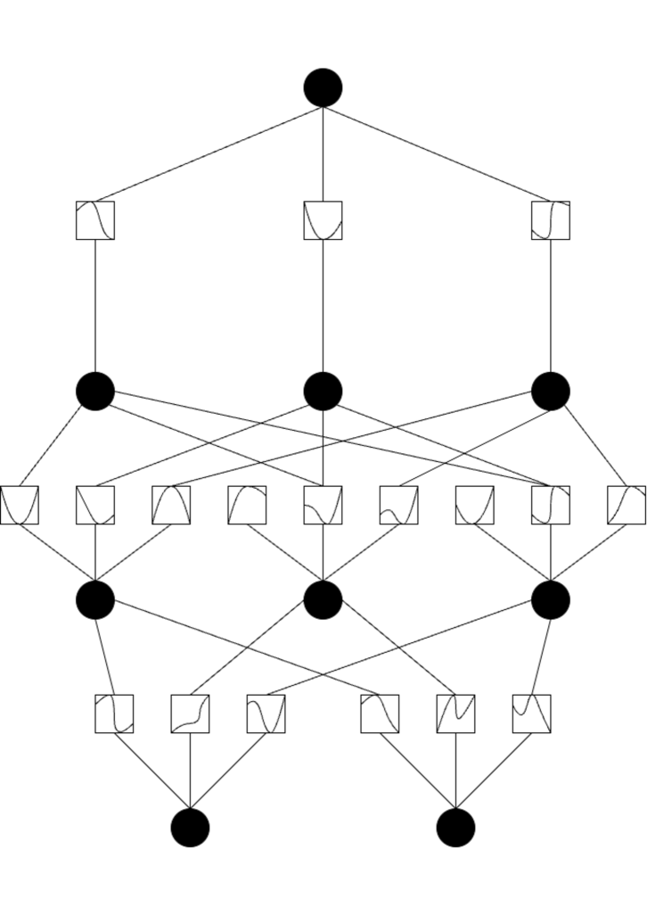
Figure 1: KAN: Kolmogorov-Arnold Networks [16]

4.1 KAN Preliminaries

KANs have recently emerged as a significant advancement in a wide range of tasks that rely on predictive algorithms at their core. While their effectiveness in supervised learning has been well-documented, to the best of our knowledge, no work has yet explored their application to causal inference. The foundation of KANs lies in the Kolmogorov-Arnold Representation Theorem [5], which states that any smooth function $f:[0,1]^{n}\to\mathbb{R}$ can be expressed as:

$$f(x_{1},\dots,x_{n})=\sum_{q=1}^{2n+1}\Phi_{q}\left(\sum_{p=1}^{n}\phi_{q,p}(x_{p})\right),$$ (5)

where $\phi_{q,p}:[0,1]\rightarrow\mathbb{R}$ and $\Phi_{q}:\mathbb{R}\rightarrow\mathbb{R}.$ This formulation demonstrates that multivariate functions can be fundamentally decomposed into a sum of univariate functions, making the composition purely additive. This theorem serves as the inspiration for the KAN architecture, originally proposed for supervised learning tasks. In such tasks, the goal is to model a function $f$ based on input-output pairs $\{(\mathbf{x}_{i},y_{i})\}$, such that $y_{i}\approx f(\mathbf{x}_{i})$.

The KAN architecture as illustrated in Figure 1 is designed such that all learnable functions are univariate, with each parameterized using basis functions, such as a B-spline, to enhance the model’s flexibility. Liu et al. [16] introduced the KANs, initially proposing a two-layer model where learnable activation functions are placed on the edges, with aggregation achieved through summation at the nodes. However, this simple design had limitations in approximating complex functions. To address these shortcomings, the authors extended the approach within the same work by introducing multiple layers and increasing both the breadth and depth of the network, thereby enhancing its ability to approximate more complex functions. A KAN layer, suitable for deeper architectures, with $n_{\text{in}}$ inputs and $n_{\text{out}}$ outputs is defined by a matrix of univariate functions:

$$\Phi=\{\phi_{q,p}\},\quad p=1,2,\dots,n_{\text{in}},\quad q=1,2,\dots,n_{\text{out}},$$ (6)

where each $\phi_{q,p}$ is a trainable univariate function with adjustable parameters. This structure allows the original two-layer Kolmogorov-Arnold representation to be extended into a more robust, deeper architecture capable of handling increasingly complex tasks. With the help of the above, we now proceed to explain KANITE framework in detail in the following subsection.

Algorithm 1 KANITE Training

 Input: Observational data: $\mathcal{D}=\{\left(\mathbf{x}_{i},t_{i},Y_{t_{i}}^{i}\right)\}_{i=1}^{n}\sim\mathcal{D}_{\text{train}},\mathcal{D}_{\text{val}}$, and hyper parameters $\alpha\geq 0$ and $\beta\geq 0.$

 Output: An outcome prediction model: $f(\Psi,\Pi),$ where $\Pi=(\Pi_{1},\Pi_{2},\cdots,\Pi_{K})$

1: Initialize parameters: $\Psi:\mathtt{KAN},\Pi:\mathtt{KAN}$

2: while not converged do

3:  Sample a mini-batch $B=\{(\mathbf{x}_{i_{o}},Y^{i_{o}}_{t_{i_{o}}})\}_{o=1}^{B}\subset\mathcal{D}_{\text{train}}$

4:  Mini-batch approximation of Regression Loss $\mathcal{L}_{1}=\frac{1}{|B|}\sum\limits_{o=1}^{|B|}(\hat{Y}_{t_{i_{o}}}-Y_{t_{i_{o}}})^{2}$

5:  Mini-batch approximation of the Representation Loss $\mathcal{L}_{2}=\frac{1}{\binom{K}{2}}\sum\limits_{a=1}^{K}\sum\limits_{b=1}^{a-1}\mathrm{RepresentationLoss}\left(\Psi_{t=a},\Psi_{t=b}\right)$

6:  Update Functions: $f(\Psi,\Pi)\leftarrow f(\Psi,\Pi)-\lambda.\nabla(f({\Psi,\Pi}))$

7:  Minimize $\alpha\cdot\mathcal{L}_{1}+\beta\cdot\mathcal{L}_{2}$ using SGD

8: end while

4.2 KANITE Architecture

Our proposed KANITE framework addresses the task of ITE estimation for multiple treatments by utilizing KANs as the backbone of its architecture. Figure 2 illustrates the details of the KANITE framework, explained through the following three key steps.

• Balanced Representation of Covariates: First, KANITE aims to learn a balanced covariate representation by replacing the conventional MLPs with the KANs, shown as Representation Network in Figure 2, enabling the model to learn latent representations of covariates balanced across all treatment groups.

• Treatment Head Networks: It consists of dedicated treatment head networks, where each treatment is modeled through a separate representation using KANs, allowing greater flexibility to capture the underlying distribution of treatment outcomes.

• Representation loss: Three different representation losses have been considered in the proposed set of algorithms under KANITE. First and second losses are Maximum Mean Discrepancy (MMD) and Wasserstein, based on the Integral Probability Metric (IPM), and the third one utilizes Entropy Balancing (EB) method [27] to learn weights that minimize the Jensen-Shannon divergence, asymptotically, between all pairs of treatment groups. These three losses result into three different algorithms named KANITE-MMD, KANITE-Wass, KANITE-EB for ITE estimation.

Figure 2: KANITE Architecture

This approach enables us to utilize the KANs for the ITE estimation task in an effective manner while simultaneously learning covariate and treatment representations that improve upon state-of-the-art (SOTA) ITE estimation algorithms. A detailed explanation of the KANITE framework is as follows.

4.2.1 KANs for learning balanced covariate representation

In earlier ITE estimation literature, representation learning for covariates has demonstrated a significant improvement [22]. In the KANITE architecture, we utilize a KAN layer setup for achieving a balanced representation that caters to multiple treatment scenarios. KAN Layers, as expressed in Equation 6, allow the architecture to learn a symbolic representation for covariates in low dimensions to mitigate confounding bias. To learn representations for covariates, $\mathbf{x}\in\mathcal{X}$, we employ KAN layers setup with learnable activation functions consist of B-Splines that learns a balanced representation function, $\Psi:\mathcal{X}\rightarrow\mathbb{R}^{d}$, in a lower-dimensional latent space.

In KANITE, a deep representation network is constructed by stacking multiple KAN layers one after the other to form a hierarchical model for representation learning. Let $L$ denote the total number of KAN layers. For each layer $l\in\{0,1,\cdots,L-1\},$ let $n_{l}$ represent the total number of neurons in layer $l.$ Let $\Psi^{l}(\mathbf{x})=\left(\Psi^{l}_{1}(\mathbf{x}),\Psi^{l}_{2}(\mathbf{x}),\cdots,\Psi^{l}_{n_{l}}(\mathbf{x})\right)$ denote the representation after the $(l-1)^{\text{st}}$ layer, with the input defined as $\Psi^{0}(\mathbf{x})=\mathbf{x}$. In contrast to standard MLPs, KANs do not learn independent weight or bias parameters; instead, each layer aggregates the outputs of learnable univariate activation functions. The transformation at layer $l\in\{0,1,...,L-1\},$ denoted as $\Psi^{l+1}(\mathbf{x})=\left(\Psi^{l+1}_{1}(\mathbf{x}),\Psi^{l+1}_{2}(\mathbf{x}),\cdots,\Psi^{l+1}_{n_{l+1}}(\mathbf{x})\right),$ is defined in a compositional form analogous to the Kolmogorov–Arnold representation as follows:

$$\Psi^{l+1}_{i}(\mathbf{x})=\sum_{j=1}^{n_{l}}\phi^{l}_{i,j}\left(\Psi^{l}_{j}(\mathbf{x})\right),\quad\forall i\in\{1,2,\cdots,n_{l+1}\}.$$ (7)

Using the recursion, we can write the above as:

$$\Psi^{l+1}(\mathbf{x})=\left(\Psi^{l}\circ\Psi^{l-1}\circ\cdots\circ\Psi^{1}\circ\Psi^{0}\right)\mathbf{x}.$$ (8)

This recursive formulation enables the deeper architecture to capture complex, non-linear interactions among covariates, progressively refining the balanced representation and further mitigating confounding bias for improved treatment effect estimation.

4.2.2 Treatment Head Networks

The KANITE framework leverages a balanced covariate representation learned from the representation network to drive the treatment head networks for enhanced treatment-specific ITE estimation. As depicted in the KANITE architecture, we deploy a distinct treatment head network for each unique treatment category. Deep KAN layers, given in Equation 8, are trained to learn a symbolic representation function that is specific to treatments. We denote these treatment head networks by $\Pi_{t}$ for $t\in\{1,2,3,\cdots,K\}$, where $K$ is the total number of unique treatments. Consider a user with covariates $\mathbf{x}$ and the assigned treatment as $t$, the treatment head network $\Pi_{t}$ with $M$ number of layers is defined as:

$$\Pi^{M+1}_{t}(\mathbf{x})=\left(\Pi^{M}_{t}\circ\Pi^{M-1}_{t}\circ\cdots\circ\Pi^{1}_{t}\circ\Pi^{0}_{t}\right)\Psi(\mathbf{x}),$$ (9)

where $\Psi(\mathbf{x})$ is the balanced representation of covariates learned from the representation network. Furthermore, we leverage network sparsification in KANs to reduce the impact of redundant activation functions, which acts as a form of regularization and improves ITE estimates.

4.2.3 Representation Loss

As mentioned in the previous subsections, learning a balanced covariates representation across all treatments plays a crucial role in KANITE. Hence, we employ three variations of the representation loss in KANITE based on IPM and Entropy Balancing, resulting into three different algorithms, in addition to the standard Mean Square Error (MSE) loss on the observed factual data. Note that, MSE loss is defined as: $\mathcal{L}_{1}=\frac{1}{n}\sum_{i=1}^{n}(\hat{Y}_{i,t}-Y_{i})^{2}.$ In the below we provide more details of the representation loss variants.

• IPM based representation loss:
  IPMs have shown promising results in achieving balanced representations for ITE estimation, as demonstrated in [22] and [10]. In KANITE, we leverage two popular IPM-based loss functions—the Maximum Mean Discrepancy (MMD) and the Wasserstein loss, to effectively capture distributional differences between treatment subgroups. MMD is particularly useful because it compares higher-order moments between distributions, minimizing subtle discrepancies in the feature space, while the Wasserstein metric provides a robust measure of distance even when distributions have limited overlap. For our multiple-treatment setup, we use the average pairwise IPM loss from [24] to learn a balanced representation across all treatment group combinations. The mathematical formulation is provided below:

  $$\mathcal{L}_{2}=\frac{1}{\binom{K}{2}}\sum_{a=0}^{K-1}\sum_{b=0}^{a-1}\texttt{IPM}\left(\{\Psi\}_{t=a},\{\Psi\}_{t=b}\right),$$ (10)

  where $\texttt{IPM}()$ can be either MMD or Wasserstein, leading to the respective algorithms KANITE-MMD and KANITE-Wass.

• Entropy Balancing (EB) based representation loss:

  In [27], a doubly robust representation learning approach is proposed for ITE estimation in the binary treatment setting. It uses Entropy Balancing (EB) to learn weights that, in the limit, minimize the Jensen-Shannon divergence between treated and control covariates distributions. In this work, we extend this methodology to the multiple-treatment setting to balance covariate distributions across all treatment groups, as given below.

  Let $m$ be the number of covariates. Entropy balancing optimization problem for the multiple-treatment setting to balance covariates distributions is given as:

  $$\hskip 71.13188pt\mathbf{w}^{\text{EB}}=\arg\max_{\mathbf{w}}\left\{-\sum_{i=1}^{N}w_{i}\log w_{i}\right\},$$

  $$\text{s.t.}\begin{cases}\text{(i)}\sum\limits_{T_{i}=t}w_{i}\,\Psi(x_{ji})=\sum\limits_{T_{i}=s}w_{i}\,\Psi(x_{ji}),\forall\,j\in\{1,2,\ldots,m\}\text{ and }t<s,\\[4.30554pt] \text{(ii)}\sum\limits_{T_{i}=t}w_{i}=1,\forall\,t\in\{1,2,\cdots,K\},\forall w_{i}>0.\end{cases}$$ (11)

  Note that, constraint (i) ensures that the weighted sum of the shared representations of the covariates is balanced across all pairs of treatment combinations. Then, the representation loss in this case is given as

  $$\mathcal{L}_{2}=\sum\limits_{i=1}^{N}w_{i}^{\text{EB}}(\Psi)\log(w_{i}^{\text{EB}}(\Psi)).$$ (12)

  We solve the optimization problem in (11) by formulating its dual problem using Lagrangian duality theory [3]. To that end, let us define the following: for $t<s$, $\lambda_{t,s}=[\lambda_{t,s,1},\lambda_{t,s,2},\ldots,\lambda_{t,s,m}]\in\mathbb{R}^{m}$ and set $\lambda_{t,s}=-\lambda_{s,t}\quad\text{for }t>s.$ By constructing the Lagrangian function and applying the Karush-Kuhn-Tucker (KKT) conditions we get the following dual problem of (11):

  $$\min_{\lambda_{t,s}}\sum_{t=1}^{k}\log\left(\sum_{T_{i}=t}\exp\left(-\sum_{s\neq t}\langle\lambda_{t,s},\Psi_{i}\rangle\right)\right),$$ (13)

  where $\Psi_{i}=[\Psi_{i,1},\Psi_{i,2},\ldots,\Psi_{i,m}]\in\mathbb{R}^{m}.$ Using the above dual formulation, we now provide a closed-form solution for equation (11). Suppose $T_{i}=t$; then, the weight for sample-$i$, $w_{i}$, is given by:

  $$w_{i}=\frac{\exp\left(-\sum_{s\neq t}\langle\lambda_{t,s},\Psi_{i}\rangle\right)}{\sum_{T_{i}=t}\exp\left(-\sum_{s\neq t}\langle\lambda_{t,s},\Psi_{i}\rangle\right)}.$$ (14)

  This formulation provides a principled approach to deriving weights using the EB method that, in the limit, minimize the JSD. We refer to the algorithm that employs the EB-based representation loss as KANITE-EB.

Note that the final loss function of the KANITE framework is a weighted sum of the standard MSE and the chosen representation loss (MMD, Wasserstein, or EB-based), as shown below.

$$\mathcal{L}=\alpha\cdot\mathcal{L}_{1}+\beta\cdot\mathcal{L}_{2}\quad\text{for some}\,\alpha,\beta>0.$$

5 Experiments

In this section, we present a detailed numerical analysis of KANITE’s performance on several standard benchmark datasets —IHDP [22], NEWS [21], TWINS [1], and ACIC-16 [6] —compared to baselines. We first evaluate KANITE against baselines using the metrics $\epsilon_{\text{PEHE}}$ and $\epsilon_{\text{ATE}}$, as defined in Equations (3) and (4). Next, we examine its convergence and parameter efficiency relative to the baselines. Finally, we analyze the impact of hyperparameters, such as grid size and spline degree in activation functions of KAN layers, on ITE estimation.

5.1 Baselines

We compare KANITE with various baseline architectures designed for ITE estimation in both binary and multiple-treatment settings. For the multiple-treatment evaluation, we use the NEWS-4, NEWS-8, and NEWS-16 semi-synthetic datasets from [21], while for binary treatment setting, we consider the IHDP, TWINS, ACIC-16, and NEWS-2 datasets. The models we benchmark against include TarNet, CFRNet-Wass, and CFRNet-MMD [22] which utilize IPM as the representation loss. We also introduce a baseline called CFRNet-EB, which uses the Entropy Balancing loss, as given in Equation (12), in place of IPM within the CFRNet architecture. For a fair comparison in the multiple-treatment setting, we also compare KANITE with Perfect Match [21]. Additionally, to benchmark against generative counterfactual predictive models, we evaluate GANITE [26]. Since KANITE operates in both binary and multiple treatment scenarios, we appropriately modify baselines developed for binary treatment setting, such as TarNet, CFRNet-Wass, CFRNet-MMD and CFRNet-EB to ensure a fair comparison across both treatment setups.

Table 1: Performance comparison of KANITE vs baselines on $\epsilon_{\text{PEHE}}$ metric across various binary treatment setting datasets

Method/Dataset	IHDP	NEWS-2	TWINS	ACIC-16
TarNet	2.33 $\pm$ 2.71	23.90 $\pm$ 8.75	0.32 $\pm$ 0.00	2.41 $\pm$ 0.91
CFRNet-Wass	1.50 $\pm$ 1.76	23.85 $\pm$ 6.24	0.32 $\pm$ 0.00	2.58 $\pm$ 1.05
CFRNet-MMD	1.50 $\pm$ 1.73	23.14 $\pm$ 7.10	0.32 $\pm$ 0.00	2.42 $\pm$ 0.88
CFRNET-EB	1.22 $\pm$ 1.32	21.25 $\pm$ 5.33	0.43 $\pm$ 0.20	2.89 $\pm$ 1.44
PerfectMatch	1.56 $\pm$ 1.71	23.18 $\pm$ 8.13	0.32 $\pm$ 0.00	2.48 $\pm$ 0.89
GANITE	7.91 $\pm$ 7.47	23.22 $\pm$ 8.38	0.35 $\pm$ 0.07	5.24 $\pm$ 1.38
KANITE-Wass	1.08 $\pm$ 1.39	20.78 $\pm$ 3.59	0.32 $\pm$ 0.00	1.58 $\pm$ 1.09
KANITE-MMD	1.08 $\pm$ 1.39	20.78 $\pm$ 3.61	0.32 $\pm$ 0.00	1.58 $\pm$ 1.09
KANITE-EB	1.08 $\pm$ 1.39	20.32 $\pm$ 2.82	0.32 $\pm$ 0.00	1.58 $\pm$ 1.09

Table 2: Performance comparison of KANITE vs baselines on $\epsilon_{\text{ATE}}$ metric across various binary treatment setting datasets

Method/Dataset	IHDP	NEWS-2	TWINS	ACIC-16
TarNet	0.63 $\pm$ 0.83	11.85 $\pm$ 11.50	0.02 $\pm$ 0.01	0.30 $\pm$ 0.16
CFRNet-Wass	0.24 $\pm$ 0.25	11.61 $\pm$ 9.48	0.02 $\pm$ 0.01	0.54 $\pm$ 0.20
CFRNet-MMD	0.24 $\pm$ 0.24	10.85 $\pm$ 9.73	0.01 $\pm$ 0.01	0.37 $\pm$ 0.32
CFRNET-EB	0.29 $\pm$ 0.34	7.71 $\pm$ 7.46	0.22 $\pm$ 0.28	0.37 $\pm$ 0.19
PerfectMatch	0.25 $\pm$ 0.25	10.34 $\pm$ 10.64	0.03 $\pm$ 0.01	0.39 $\pm$ 0.29
GANITE	4.40 $\pm$ 1.33	11.28 $\pm$ 10.80	0.35 $\pm$ 0.07	3.61 $\pm$ 1.07
KANITE-Wass	0.15 $\pm$ 0.13	7.03 $\pm$ 5.43	0.01 $\pm$ 0.00	0.18 $\pm$ 0.13
KANITE-MMD	0.15 $\pm$ 0.13	7.02 $\pm$ 5.48	0.01 $\pm$ 0.00	0.19 $\pm$ 0.14
KANITE-EB	0.15 $\pm$ 0.13	6.38 $\pm$ 4.49	0.01 $\pm$ 0.00	0.18 $\pm$ 0.13

Table 3: Performance comparison of KANITE vs baselines on $\epsilon_{\text{PEHE}}$ metric across various multiple treatment setting datasets

Method/Dataset	NEWS-4	NEWS-8	NEWS-16
TarNet	24.09 $\pm$ 4.07	24.85 $\pm$ 6.73	25.06 $\pm$ 2.96
CFRNet-Wass	24.98 $\pm$ 4.57	22.70 $\pm$ 3.39	22.60 $\pm$ 1.75
CFRNet-MMD	24.05 $\pm$ 4.56	23.17 $\pm$ 3.32	22.81 $\pm$ 1.63
CFRNET-EB	21.71 $\pm$ 2.63	22.53 $\pm$ 3.13	22.33 $\pm$ 1.69
PerfectMatch	23.90 $\pm$ 4.60	23.41 $\pm$ 4.20	23.33 $\pm$ 1.68
GANITE	23.77 $\pm$ 4.10	24.10 $\pm$ 3.33	22.85 $\pm$ 1.62
KANITE-Wass	21.48 $\pm$ 2.27	22.48 $\pm$ 3.31	22.20 $\pm$ 1.57
KANITE-MMD	21.53 $\pm$ 2.31	22.58 $\pm$ 3.37	22.19 $\pm$ 1.57
KANITE-EB	21.52 $\pm$ 2.30	22.62 $\pm$ 3.38	22.20 $\pm$ 1.58

Table 4: Performance comparison of KANITE vs baselines on $\epsilon_{\text{ATE}}$ metric across various multiple treatment setting datasets

Method/Dataset	NEWS-4	NEWS-8	NEWS-16
TarNet	11.87 $\pm$ 5.07	10.91 $\pm$ 3.49	12.47 $\pm$ 3.01
CFRNet-Wass	13.33 $\pm$ 5.56	9.08 $\pm$ 3.55	9.08 $\pm$ 1.96
CFRNet-MMD	11.43 $\pm$ 5.64	9.98 $\pm$ 3.37	9.09 $\pm$ 1.88
CFRNET-EB	8.26 $\pm$ 3.29	9.03 $\pm$ 3.10	9.08 $\pm$ 1.92
PerfectMatch	11.43 $\pm$ 5.71	9.62 $\pm$ 3.63	8.85 $\pm$ 1.99
GANITE	11.65 $\pm$ 5.03	11.74 $\pm$ 3.50	10.54 $\pm$ 1.77
KANITE-Wass	7.92 $\pm$ 2.97	8.91 $\pm$ 3.09	9.49 $\pm$ 1.84
KANITE-MMD	8.05 $\pm$ 2.95	9.24 $\pm$ 3.45	9.46 $\pm$ 1.84
KANITE-EB	8.03 $\pm$ 2.93	9.30 $\pm$ 3.48	9.47 $\pm$ 1.85

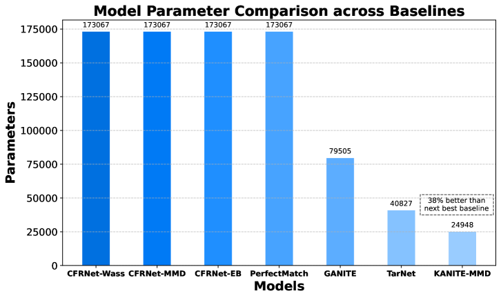
(a) Comparison of model parameters

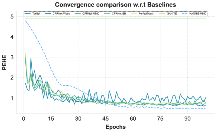
(b) Comparison of model convergence

Figure 3: Comparison of model parameters and convergence across models

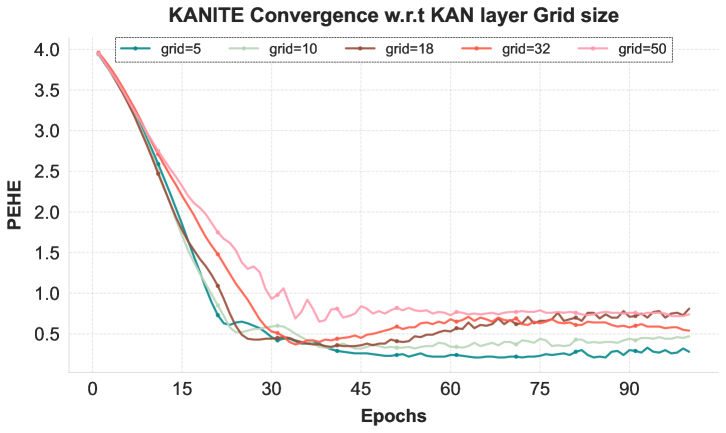
(a) Affect of grid size

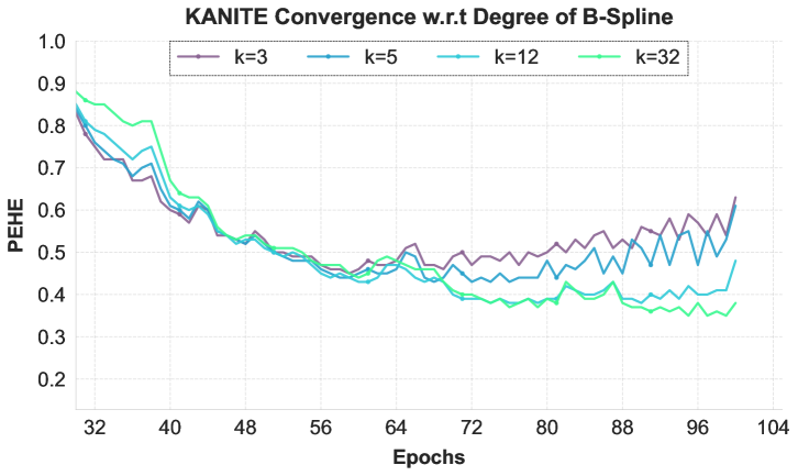
(b) Affect of spline degree

Figure 4: Affect of grid size and spline degree considered in KANITE on ITE

5.2 KANITE: Performance Assessment

We split the dataset into training, validation, and test sets in a 63:27:10 ratio. The results in all tables are computed on the full dataset after model training. We conducted 1000, 50, 10, and 10 iterations for the IHDP, NEWS, TWINS, and ACIC-16 datasets, respectively, and report the mean and standard deviation of these runs in the results tables. The best results in the tables are highlighted in bold.

As mentioned earlier, the KANITE framework consists of three algorithms: KANITE-MMD, KANITE-Wass, and KANITE-EB, almost at least one of which outperforms all the baselines on both $\epsilon_{\text{PEHE}}$ and $\epsilon_{\text{ATE}}$ metrics in both binary and multiple treatment settings, as shown in Table 1, 2, 3, and 4. Note that Tables 1 and 2 present the $\epsilon_{\text{PEHE}}$ and $\epsilon_{\text{ATE}}$ metrics for all considered algorithms in the binary treatment setting, respectively. Similarly, Tables 3 and 4 provide the corresponding results for the multiple-treatment setting. To perform a comprehensive performance assessment of KANITE, we evaluate its convergence and parameter efficiency compared to the baselines. Figure 3(a) compares the number of parameters in our proposed KANITE framework against all baselines. Notably, KANITE outperforms all baselines on both $\epsilon_{\text{PEHE}}$ and $\epsilon_{\text{ATE}}$ metrics while reducing model parameters by 38% compared to the next best baseline. Figure 3(b) shows that our proposed KANITE model, depicted in dotted line, converges faster than all baselines. Since all three KANITE variants exhibited similar behavior in terms of parameter count and convergence, we present only KANITE-MMD in Figure 3 to keep the figures uncluttered.

5.3 KANITE: Hyperparameters study

We now examine the impact of the B-Spline degree and grid size considered in KAN layers on model performance. As grid size and spline degree are direct proportional to the model complexity in terms of parameters we conduct the hyperparameter optimization on them and use the best parameters in the respective models. For example, Figure 4 shows the affect of grid size and spline degree on the ITE estimates for IHDP dataset. From Figure 4, it can be observed that grid size of 5 and spline degree of 32 achieve the best performance on this iteration of the results.

6 Conclusion

In this study, we proposed KANITE, a state-of-the-art framework for ITE estimation that leverages shared representation learning using either IPM or Entropy Balancing. Unlike traditional MLP-based architectures, KANITE employs KANs as its backbone, enabling it to learn more accurate causal effect estimates. The framework introduces three algorithms—KANITE-MMD, KANITE-Wass, and KANITE-EB—each utilizing a different IPM or Entropy Balancing-based representation loss to ensure balanced covariate representations across treatment groups. Additionally, we derive a closed-form Entropy Balancing-based representation loss for the multiple-treatment setting using Lagrangian duality theory. Experimental results demonstrate that KANITE effectively handles multiple-treatment scenarios, outperforming all considered baselines on both the $\epsilon_{\text{PEHE}}$ and $\epsilon_{\text{ATE}}$ metrics. Furthermore, KANITE achieves superior parameter efficiency and faster convergence while maintaining strong counterfactual prediction capabilities.

For future work, we plan to further enhance KANITE to create a unified architecture that incorporates abilities of both IPM and Entropy Balancing for ITE estimation tasks. We plan to incorporate interpretability of KANs to understand causal effects estimation in a better manner. Our findings highlight the advantages of KANs in ITE estimation, paving the way for future research in related areas. One promising direction is investigating the role of KANs in ITE estimation under networked settings, where users are interconnected through a network [24]. Another avenue is examining the effectiveness of KANs in treatment dosage settings, where treatments are administered in fractional amounts between 0 and 1 [20]. Additionally, it would be valuable to study how KANs can improve causal effect estimation when incorporating treatment information [8].

References

- [1] Almond, D., Chay, K.Y., Lee, D.S.: The costs of low birth weight. The Quarterly Journal of Economics 120(3), 1031–1083 (2005)
- [2] Bodner, A.D., Tepsich, A.S., Spolski, J.N., Pourteau, S.: Convolutional kolmogorov-arnold networks. arXiv preprint arXiv:2406.13155 (2024)
- [3] Boyd, S.P., Vandenberghe, L.: Convex optimization. Cambridge university press (2004)
- [4] Braun, J., Griebel, M.: On a constructive proof of kolmogorov’s superposition theorem. Constructive approximation 30, 653–675 (2009)
- [5] Braun, J., Griebel, M.: On a constructive proof of kolmogorov’s superposition theorem. Constructive Approximation 30, 653–675 (2009), https://api.semanticscholar.org/CorpusID:5164789
- [6] Dorie, V., Hill, J., Shalit, U., Scott, M., Cervone, D.: Automated versus do-it-yourself methods for causal inference: Lessons learned from a data analysis competition. Statistical Science 34(1), 43–68 (2019)
- [7] Guo, R., Li, J., Liu, H.: Learning individual causal effects from networked observational data. In: Proceedings of the 13th international conference on web search and data mining. pp. 232–240 (2020)
- [8] Harada, S., Kashima, H.: Graphite: Estimating individual effects of graph-structured treatments. In: Proceedings of the 30th ACM International Conference on Information & Knowledge Management. pp. 659–668 (2021)
- [9] Hornik, K., Stinchcombe, M., White, H.: Multilayer feedforward networks are universal approximators. Neural networks 2(5), 359–366 (1989)
- [10] Johansson, F., Shalit, U., Sontag, D.: Learning representations for counterfactual inference. In: International conference on machine learning. pp. 3020–3029. PMLR (2016)
- [11] Kaddour, J., Zhu, Y., Liu, Q., Kusner, M.J., Silva, R.: Causal effect inference for structured treatments. Advances in Neural Information Processing Systems 34, 24841–24854 (2021)
- [12] Kiamari, M., Kiamari, M., Krishnamachari, B.: Gkan: Graph kolmogorov-arnold networks. arXiv preprint arXiv:2406.06470 (2024)
- [13] Kich, V.A., Bottega, J.A., Steinmetz, R., Grando, R.B., Yorozu, A., Ohya, A.: Kolmogorov-arnold networks for online reinforcement learning. In: 2024 24th International Conference on Control, Automation and Systems (ICCAS). pp. 958–963. IEEE (2024)
- [14] Kolmogorov, A.: On the representation of continuous functions of several variables by superpositions of continuous functions of a smaller number of variables
- [15] Kolmogorov, A.N.: On the representations of continuous functions of many variables by superposition of continuous functions of one variable and addition. In: Dokl. Akad. Nauk USSR. vol. 114, pp. 953–956 (1957)
- [16] Liu, Z., Wang, Y., Vaidya, S., Ruehle, F., Halverson, J., Soljačić, M., Hou, T.Y., Tegmark, M.: Kan: Kolmogorov-arnold networks. arXiv preprint arXiv:2404.19756 (2024)
- [17] Moradi, M., Panahi, S., Bollt, E., Lai, Y.C.: Kolmogorov-arnold network autoencoders. arXiv preprint arXiv:2410.02077 (2024)
- [18] Nilforoshan, H., Moor, M., Roohani, Y., Chen, Y., Šurina, A., Yasunaga, M., Oblak, S., Leskovec, J.: Zero-shot causal learning. Advances in Neural Information Processing Systems 36, 6862–6901 (2023)
- [19] Rubin, D.B.: Causal inference using potential outcomes: Design, modeling, decisions. Journal of the American Statistical Association 100(469), 322–331 (2005)
- [20] Schwab, P., Linhardt, L., Bauer, S., Buhmann, J.M., Karlen, W.: Learning counterfactual representations for estimating individual dose-response curves. In: Proceedings of the AAAI Conference on Artificial Intelligence. vol. 34, pp. 5612–5619 (2020)
- [21] Schwab, P., Linhardt, L., Karlen, W.: Perfect match: A simple method for learning representations for counterfactual inference with neural networks. arXiv preprint arXiv:1810.00656 (2018)
- [22] Shalit, U., Johansson, F.D., Sontag, D.: Estimating individual treatment effect: generalization bounds and algorithms. In: International conference on machine learning. pp. 3076–3085. PMLR (2017)
- [23] Thorat, A., Kolla, R., Pedanekar, N.: I see, therefore i do: Estimating causal effects for image treatments. arXiv preprint arXiv:2412.06810 (2024)
- [24] Thorat, A., Kolla, R., Pedanekar, N., Onoe, N.: Estimation of individual causal effects in network setup for multiple treatments. arXiv preprint arXiv:2312.11573 (2023)
- [25] Yang, X., Wang, X.: Kolmogorov-arnold transformer. In: The Thirteenth International Conference on Learning Representations (2024)
- [26] Yoon, J., Jordon, J., Van Der Schaar, M.: Ganite: Estimation of individualized treatment effects using generative adversarial nets. In: International conference on learning representations (2018)
- [27] Zeng, S., Assaad, S., Tao, C., Datta, S., Carin, L., Li, F.: Double robust representation learning for counterfactual prediction. arXiv preprint arXiv:2010.07866 (2020)
- [28] Zeydan, E., Vaca-Rubio, C.J., Blanco, L., Pereira, R., Caus, M., Aydeger, A.: F-kans: Federated kolmogorov-arnold networks. arXiv preprint arXiv:2407.20100 (2024)