Is Limited Participant Diversity Impeding EEG-based Machine Learning?

Abstract

The application of machine learning (ML) to electroencephalography (EEG) has great potential to advance both neuroscientific research and clinical applications. However, the generalisability and robustness of EEG-based ML models often hinge on the amount and diversity of training data. It is common practice to split EEG recordings into small segments, thereby increasing the number of samples substantially compared to the number of individual recordings or participants. We conceptualise this as a multi-level data generation process and investigate the scaling behaviour of model performance with respect to the overall sample size and the participant diversity through large-scale empirical studies. We then use the same framework to investigate the effectiveness of different ML strategies designed to address limited data problems: data augmentations and self-supervised learning. Our findings show that model performance scaling can be severely constrained by participant distribution shifts and provide actionable guidance for data collection and ML research.

1 Main

A century after the first human electroencephalogram was recorded in 1924, Electroencephalography (EEG) is in many ways still the best available technique for the direct and non-invasive measurement of brain activity. In particular, with newer generations of dry-electrode recording hardware, it has a unique set of desirable properties, including its low cost and patient burden, portability, and high temporal resolution. Given the complexity and high dimensionality of EEG signals, machine learning (ML) has shown considerable promise in advancing neuroscientific research and clinical applications [1, 2, 3, 4]. However, the successful deployment of ML in EEG-based applications is not without challenges. A fundamental obstacle is the limited availability of high-quality EEG data, which is often sparse, noisy, and costly to collect.

While prior works have acknowledged limited data as a challenge for EEG-based machine learning [5, 6], systematic studies are currently lacking. Furthermore, an aspect that has largely been ignored is the hierarchical nature of the data generation process relevant to EEG machine learning work. EEG-based ML models rarely operate on full recordings; samples usually correspond to more manageable segments on the order of a few seconds, extracted from recordings through sliding-window approaches [5]. As a result, the overall sample size is usually considerably larger than the number of individual participants in the dataset. Many applications, particularly in a medical context, require models to generalise to new participants – e.g., a diagnostic model is of little use if it can only diagnose patients in the training data. Consequently, if there is a significant distribution shift between participants, low participant diversity could impede model performance even with a large overall sample size. Understanding the relevance of participant diversity is critical to guide data collection and future EEG-based machine learning work. If models generalise well across participants, data could be collected from smaller cohorts, significantly reducing costs and logistical challenges. Conversely, if participant diversity is crucial, this motivates not only higher participant counts during data collection, but also the development of machine learning strategies that explicitly address participant distribution shifts.

To address these challenges, we first formalise a hierarchical data generation process that captures the structure of EEG data used to train machine learning models. Furthermore, we systematically investigate the data scaling behaviour of different EEG machine learning models (TCN, mAtt, LaBraM) across a range of large datasets (TUAB, CAUEEG, PhysioNet), each with more than 1,000 participants, and three tasks (EEG normality prediction, dementia diagnosis, sleep staging). Crucially, we control both the number of participants in the training data and the amount of data per participant, allowing us to disentangle the impact of participant diversity from the overall sample size.

Beyond the collection of larger datasets, several works of research have proposed strategies to deal with limited data by making better use of available data or by transferring representations learned on other (sometimes unlabelled) datasets. Inspired by their success in computer vision, one line of research has focused on the development of data augmentations [6, 7, 8, 9], which artificially inflate the dataset size through the application of label-preserving transformations to available samples [10]. Often these transformations are designed based on prior knowledge about desirable invariances, e.g. prominent examples in computer vision like cropping or translation encourage invariance to object positions within the image [10, 11]. Moreover, the success of large language models has sparked a lot of interest in pre-training strategies based on masking and the reconstruction of raw data or latent features [12, 13, 14, 15]. Several of these works have also adopted the notion of foundation models [16]. These studies have laid valuable groundwork, often demonstrating effectiveness on smaller datasets or for particular prediction tasks. However, understanding how these approaches perform across a broader range of data settings can provide deeper insights into their generalisability and scalability.

We assess the utility of existing data augmentations (AmplitudeScaling, FrequencyShift, PhaseRandomisation) and a pre-trained foundation model (LaBraM) for varying amounts of (downstream) training data. Specifically, we quantify their effectiveness in data-limited regimes, whether they continue to provide value as the dataset size increases, and how they address specific limitations, such as low participant diversity versus limited data per participant.

In summary, we offer the following contributions:

• We formalise the data generation process for EEG-based machine learning and use recent, relevant advances in statistical learning theory to inform our experiment designs.

• We empirically study the scaling behaviour and the relevance of participant distribution shifts across different models, tasks, and datasets.

• We assess the utility of existing data augmentations and a pre-training strategy in improving model performance in different data regimes.

Our findings provide useful insights to guide data collection and the development of EEG-based machine learning methods.

2 Results

2.1 Data Generation Process and Experiment Overview

We model datasets used for EEG-based machine learning by the hierarchical data generation process illustrated in Figure 1A. A dataset comprises recordings from $n$ different participants, which are in turn segmented into $m$ distinct samples per participant. As a result, the overall sample size is usually substantially larger than the number of individual participants from which the samples are obtained. Formally, we can denote the sample features by $X_{ij}$ where $i=1,...,n$ indexes the participants, and $j=1,...,m$ indexes the samples for participant $i$, and with corresponding ground-truth labels denoted by $Y_{ij}$. For each participant, these samples follow a participant-specific distribution $P_{i}$, which is itself drawn from a population-level distribution $Q$.

Consider a loss function, $\ell(\hat{Y},Y)$, measuring the quality of a prediction, $\hat{Y}=f(X)$, provided by some model, $f$. This could be, e.g., the zero-one loss or the cross entropy loss, and need not be the loss actually used to train a model. We can define the empirical risk (measured on the training set) and population risk as

$$r(f):=\frac{1}{mn}\sum_{i=1}^{n}\sum_{j=1}^{m}\ell(f(X_{ij}),Y_{ij})$$ (1)

and

$$R(f)=\mathbb{E}_{X,Y}[\ell(f(X),Y)],$$ (2)

respectively. In the classic learning setting, where each $P_{i}$ is assumed to be the same, it is well established in the statistical learning theory literature that the gap between empirical risk and population risk (i.e., the extent to which a model will overfit) scales as $\tilde{\Theta}(1/(mn)^{p})$, where $p\in\{\frac{1}{2},1\}$ [17]. The value of $p$ will be $\frac{1}{2}$ unless some assumptions are satisfied relating to the suitability of the model architecture and the amount of information the features contain about the labels [18]. The two-level data generation process we consider is comparatively less studied, but it is known that with minimal assumptions about model choices and feature information content, the gap will scale as $\tilde{\Theta}(1/n^{\frac{1}{2}}+1/(mn)^{\frac{1}{2}})$ [19]. We include the second term, which is asymptotically dominated by the first, because if the distribution shift is small, or one is able to select a model architecture with substantial robustness to distribution shifts, then the second term can be larger in the non-asymptotic regime [19]. This analysis tells us that in the presence of a substantial distribution shift, the extent to which one should expect to overfit is governed primarily by the number of participants, rather than the amount of data available per participant, unless one is able to design a model architecture with the appropriate invariances.

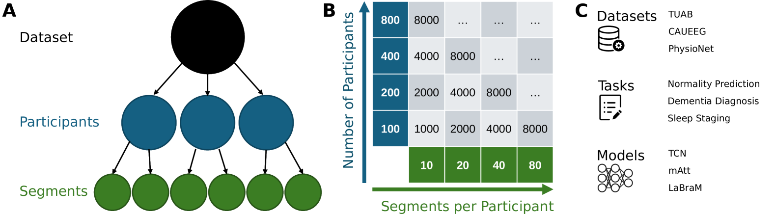
Figure 1: (A) Multi-level EEG data distribution. A dataset contains EEG recordings from multiple participants, which are usually further divided into smaller segments to train machine learning models. (B) Grid visualising the subsampling of training datasets controlling for both the number of participants and the number of segments per participant. (C) The datasets, tasks, and models used in the experiments.

We conducted data scaling experiments to empirically assess the dependence of ML model performance on the participant count $n$ and the number of samples per participant $m$ across three large datasets and prediction tasks (normality prediction on TUAB – binary classification, dementia diagnosis on CAUEEG – three-way classification, and sleep staging on PhysioNet – five-way classification; see Section 4.2). Starting from the full datasets, we randomly subsampled training datasets with a fixed number of participants and overall sample size as visualised by the grid depicted in Figure 1B. Different ML models (TCN – a convolutional neural network, mAtt – a geometric deep learning approach, and LaBraM – a transformer architecture; see Section 4.3) were then trained on the subsampled training data. Early stopping was used to prevent overfitting with limited amounts of training data, while still allowing training to converge for larger training datasets. See Section 4.1 for more details on the experimental setup and model training.

2.2 Scaling Behaviour of Model Performance

Figure 2 depicts model accuracies for a fixed number of segments per participant ($m=40$) and shows how performance scaled with increasing sample size (specifically participant count) across the different datasets. While the shapes of the curves align with expectations from a machine learning perspective, it is informative to look at the magnitude of improvements and the participant counts at which they started to diminish.

Focusing first on the general trend across models, we observe strong improvements in accuracy as the participant count increased from 25 to several hundred participants across all datasets. To put this into context, [5] have reported the sizes of datasets used across the 154 studies included in their review of deep learning-based EEG work [5]. Astonishingly, half of the datasets contained data from less than 13 participants and only six comprised more than 250 participants. Although this might have changed since the review’s publication in roy_deep_2019, it indicates that a substantial proportion of EEG datasets fall into the range where a scarcity of participants is likely a critical limiting factor. In such cases, substantial gains could be achieved through the collection of additional training data from more participants.

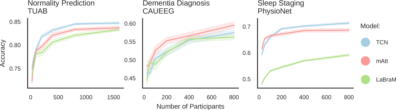
Figure 2: Scaling behaviour of model performance. Average accuracies of the different models for normality prediction on TUAB, dementia diagnosis on CAUEEG, and sleep staging on PhysioNet for increasing participant counts at a fixed number of segments per participant ($m=40$). Averages were computed across seeds used to subsample the training datasets and the shading illustrates the standard error of the mean. Across all datasets, performance increased strongly as the size was increased to several hundred participants, after which improvements started to diminish.

Focusing on the right hand side of each plot, towards the maximum participant counts, accuracy improvements started to diminish. While performance appears not to have fully saturated across the three tasks, meaningful further improvements through the collection of additional labelled training data are likely infeasible. For example, recruiting an additional 1,600 participants to double the number of participants will often be prohibitively expensive for an expected improvement in performance of roughly 1%.

2.3 Model Comparison

One aspect determining the sample efficiency of a model is its architecture. We observe that the TCN and mAtt architectures performed slightly better than LaBraM on TUAB and CAUEEG and markedly better on PhysioNet. On PhysioNet, LaBraM’s substantially lower performance can partially be attributed to differences in preprocessing. As explained in Section 4.2.4, 15 second epochs had to be used for LaBraM instead of the 30 second epochs used for TCN and mAtt. We performed an ablation study where the TCN model was trained using the same preprocessing, which showed that differences in preprocessing explained part of the performance gap, but that TCN still outperformed the LaBraM model (see Section A.2). We hypothesise that LaBraM’s lower performance stems from the weaker inductive bias of the transformer architecture and the fact that the LaBraM model is considerably larger in terms of the number of model parameters compared to the other models. The LaBraM model would thus be expected to be less sample efficient.

The differences between mAtt and TCN could reflect the usefulness of different priors for different tasks. TCN, as a convolutional neural network, is likely better at picking up on specific wave morphologies (e.g. sharp waves or K-complexes), which may be useful for normality prediction and sleep staging. The mAtt model, on the other hand, embeds the EEG into a sequence of covariance matrices that reflect signal power and cross-channel correlations, and might excel in tasks where these are the most relevant features.

On the whole, and with the exception of LaBraM’s performance on PhysioNet, the achieved accuracies were relatively similar, despite substantial differences in the architectures and model sizes. The sample size was the primary driver of performance.

2.4 Participant Distribution Shifts

So far, we only varied the number of participants ($n$) and kept the number of segments per participant ($m$) fixed. Improvements in performance were therefore expected irrespective of the presence of participant distribution shifts. Figure 3 now illustrates the performance of the TCN model when controlling for both $m$ and $n$. Note that the diagonals extending from the top left to the bottom right of each heatmap correspond to fixed overall sample sizes. Moving from the bottom right along the diagonal towards the top left corresponds to the same overall sample size where data was sampled from a higher number of individual participants, i.e. higher participant diversity.

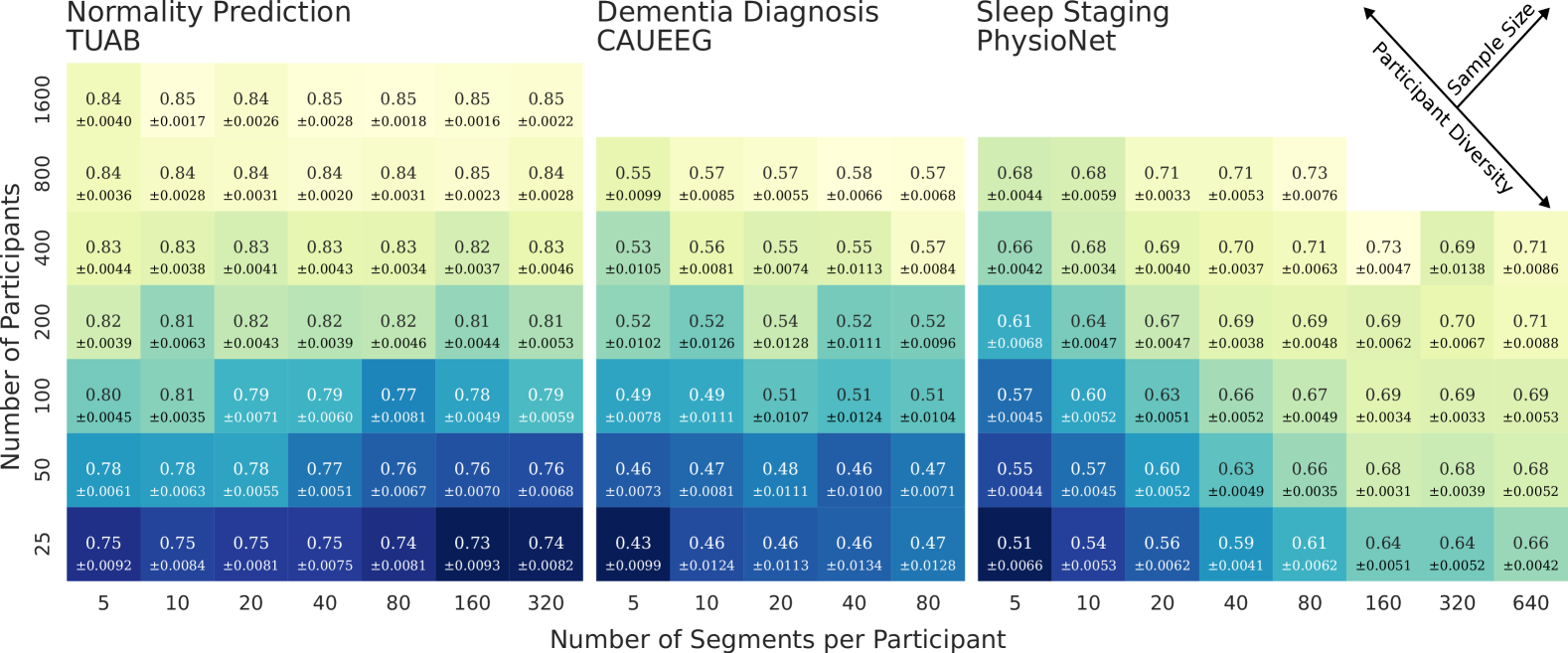
Figure 3: Differential effects of participant count and overall sample size on model performance. Accuracies of the TCN model for normality prediction on TUAB, dementia diagnosis on CAUEEG, and sleep staging on PhysioNet averaged across seeds, along with the standard error of the mean. Performance on TUAB and CAUEEG was dominated by the participant count. Sleep staging performance on PhysioNet was more dependent on the overall sample size and competitive performance was achieved even with very limited participant counts.

Focusing first on the normality prediction task on the TUAB dataset, we observe that increasing the amount of data for a fixed participant count (moving along the horizontal axis) did not yield any substantial performance improvements. However, performance was highly dependent on the participant count (moving along the vertical axis). Even for a fixed sample size, higher participant diversity yielded significant improvements (moving diagonally towards the top left). The results for the dementia prediction task on the CAUEEG dataset exhibit a similar pattern. Linking back to the theoretical analysis in Section 4.1, this suggests a substantial distribution shift between participants such that the participant count $n$ dominated model generalisation.

For the sleep staging task on the PhysioNet dataset the pattern is different. While higher participant diversity still yielded some improvements in performance (moving diagonally towards the top left), substantial improvements were also achieved by increasing the sample size for a fixed participant count (moving along the horizontal axis). In fact, with the maximum number of samples per participant, training data from a small cohort of just 25 participants was sufficient to match the performance achieved with training data from 400 participants (with 5 segments per participant).

Results for the mAtt model revealed the same patterns. For LaBraM, performance improvements for additional samples at a fixed participant count did not diminish as drastically, which is likely due to its lower sample efficiency as hypothesised in Section 2.3. Heatmaps for both models can be found in Section A.1.

2.5 Effectiveness of EEG Data Augmentation

Figure 4 illustrates the effect of different data augmentations chosen based on their promising performance in prior work (AmplitudeScaling – channel-wise multiplication with a random factor between 0.5 and 2, FrequencyShift – random shift in the frequency domain of up to 0.3 Hz, PhaseRandomization – randomisation of the phase of each Fourier coefficient; see Section 4.4).

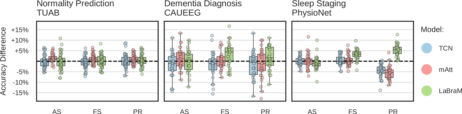
Figure 4: Impact of data augmentations. Each boxplot shows pairwise accuracy differences between augmented and unaugmented training (positive means augmentation improved performance) across all combinations of participant counts ($n$) and segments per participant ($m$). Results for only a single seed are shown for better visibility. AS = AmplitudeScaling, FS = FrequencyShift, PR = PhaseRandomization. On PhysioNet, the LaBraM model benefitted from FS and PR, whereas PR decreased performance for TCN and mAtt. Other than that, augmentations did not lead to consistent improvements in performance.

With one exception, the impact of the different augmentations was generally small and inconsistent. What stood out, however, was a systematically detrimental effect of the PhaseRandomization augmentation on PhysioNet for the TCN and mAtt models, whereas performance for the LaBraM model was improved. LaBraM also benefitted from the FrequencyShift augmentation on PhysioNet. In terms of absolute performance, LaBraM performed substantially worse on PhysioNet without data augmentation (see Figure 2), such that with data augmentation, all models performed about equally well. The observed performance improvements for LaBraM can therefore likely be attributed to its greater reliance on large amounts of data, which is partially offset by augmentation. Decreased performance in the smaller and more data-efficient models suggests that PhaseRandomization destroys useful information.

The PhaseRandomization augmentation randomises the phase of each Fourier coefficient and is applied channel-wise. It therefore preserves the power distribution across different frequencies, but completely destroys wave morphologies and cross-channel correlations. Given that certain wave forms are highly informative of the sleep stage (e.g. K-complexes are known to occur during NREM 2 sleep), the performance decreases are certainly plausible.

2.6 Effectiveness of Self-supervised Pre-training

Figure 5 shows a comparison of the LaBraM model performance with and without pre-training. LaBraM was designed as an EEG foundation model and pre-trained in an unsupervised manner (i.e. without using labels) on a diverse collection of 16 datasets ranging from brain computer interface (BCI) datasets to emotion recognition and resting state data [14]. In total, these datasets contained around 500 participants. After pre-training, the model was fine-tuned with the labelled training data of the corresponding task. The baseline model (without pre-training) was directly trained on the labelled training data from scratch. See Section 4.5 for details.

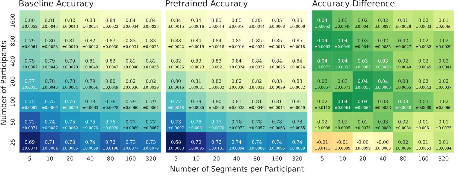
Figure 5: Effectiveness of self-supervised pre-training. Comparison of LaBraM performance with and without pre-training on TUAB. The left and middle heatmaps show average accuracies (± standard error of the mean) for LaBraM trained from scratch (baseline) and pre-trained on a collection of 16 datasets before fine-tuning on TUAB, respectively. The right heatmap visualises the average of pairwise accuracy differences (± standard error of the mean), where pairs correspond to the accuracies of pre-trained and baseline models for the same seed. pre-training consistently improved performance across all data regimes, except when the amount of fine-tuning data was most severely limited.

Pre-training consistently improved model performance across all data regimes, except when the amount of downstream fine-tuning data was most severely limited. Comparing columns in the left two heatmaps showing accuracies for the baseline (trained from scratch) and pre-trained model respectively, the effect of pre-training looks like a boost in the amount of data per participant: with only 10-20 segments per participant, the pre-trained model achieved the same performance as the baseline model with the maximum amount of 320 segments per participant. However, pre-training also improved performance when the participant count was low and it continued to provide value even when the maximum amount of data was used. Consistent results were observed for dementia prediction on the CAUEEG dataset and sleep staging on PhysioNet (see Section A.3).

In Section 2.2, we observed that the LaBraM model required substantially more data to achieve the same performance as the mAtt and TCN models. With pre-training, however, the much larger and more data-demanding LaBraM model was able to match or even outperform them. This can be seen by comparing the heatmaps in Figure 5 to the corresponding heatmap on TUAB of the TCN model in Figure 3. Alternatively, Section A.2 shows a version of Figure 2 with additional lines for the pre-trained LaBraM model.

3 Discussion

The present study demonstrates that the generalisability of EEG-based machine learning models to data from new participants is highly task-dependent. We observe that good model performance can be achieved with a relatively small number of participants in sleep staging, whereas performance in EEG normality prediction and dementia diagnosis was bottlenecked by the participant count. While our findings, therefore, do not admit a general conclusion—participant diversity is neither always the limiting factor nor universally unimportant—they highlight the importance of understanding its role in specific contexts. We recommend the conduction of pilot studies or review of prior application-specific work to inform the extent to which participant diversity should be prioritised in data collection and methodological machine learning work.

The use of large datasets allowed us to study the scaling behaviour of machine learning models over a large range of data regimes. Across all datasets, tasks, and models, we observed strong improvements in performance as the participant count was increased from 25 to several hundred participants. This highlights the value of initiatives like AI-Mind [20], a collaboration of 15 academic and industry partners pioneering a large study involving 1,000 participants with mild cognitive impairment. However, as participant counts approached the maximum sizes explored in our study, performance improvements began to diminish. While the majority of current EEG-based machine learning work still operates on smaller datasets, it is thus possible that further performance improvements through the collection of even larger labelled datasets will become prohibitively expensive. Complementary approaches, such as machine learning strategies explicitly designed to address participant distribution shifts and make more effective use of limited EEG data could become essential.

Based on these findings, we assessed the effectiveness of existing machine learning strategies for dealing with limited participant diversity and data per individual participant. In contrast to other areas where ML is used, data augmentations did not prove effective as a strategy to deal with limited participant diversity or overall sample size. It is important to note that our experimental setup considered only existing EEG data augmentation methods; we do not exclude the possibility that more effective augmentations can be designed. In fact, our results encourage the development of augmentations that specifically imitate participant differences.

Self-supervised pre-training consistently improved model performance across all data regimes. These results are particularly promising considering the broad potential for further improvements: This study benchmarked LaBraM Base, the smallest version of the model for which weights were made publicly available by the authors. Further improvements are thus likely achievable with increased model size as indicated by comparisons of the model versions in the original publication [14] as well as generally observed trends in self-supervised learning [21]. Moreover, the data used to pre-train LaBraM is still relatively limited with a total participant count of around 500—less than a third of the maximum number of participants used in our evaluations on the TUAB dataset. The existing body of literature on self-supervised learning strongly suggests that more data would result in better performance [21]. Since pre-training does not require labelled data, the creation of a larger pre-training datasets is comparatively easy. Prior work has also shown that self-supervised learning can be used to enforce approximate invariances [22], which can help circumvent the poor dependence of overfitting behaviour on the number of participants in the training data [19].

Beyond augmentations and self-supervised learning, refined preprocessing methods could provide another approach to dealing with limited EEG data by improving data quality instead of quantity. There is a rich literature on EEG preprocessing [23, 24, 25], although most methods were designed for classical EEG analysis and it is unclear how well they translate to ML-based EEG applications. Some work suggests that even with large datasets, machine learning models still benefit in particular from the removal of high-amplitude artefacts [26, 27].

Finally, future research should attempt to determine the nature of participant distribution shifts. We observed a large participant count to be critical for model performance in EEG normality prediction and EEG-based dementia diagnosis, and we can see several plausible underlying reasons. On the one hand, anatomical individual differences could impede the generalisability of the observed patterns of scalp activity measured with EEG. On the other hand, the distribution shift might also be explained by variability in how the target presents in different participants. For instance, in the EEG normality prediction task, there are numerous reasons why an EEG can be abnormal, ranging from focal epileptiform discharges to diffuse slowing. A model that is trained on data from only a small cohort of participants will therefore not only be exposed to little demographic and anatomical variation but also to a limited number of target (or disease) phenotypes. This could be particularly relevant, e.g., in the context of neurodegenerative or psychiatric diseases, where substantial individual differences in symptomatology and neural correlates have been described [28, 29].

4 Methods

4.1 Experimental Design and Model Training

Each dataset was split into train, validation, and test splits such that participants did not overlap between the splits. To study the impact of the amount and participant diversity of the training data, each experiment consisted of a grid of trials where we varied the number of participants and the number of segments per participant. Training data for each configuration was chosen through random sub-sampling from the train split (see Figure 1). To obtain uncertainty estimates, each trial was repeated multiple times with different random seeds for the data sub-sampling.

Models were trained using AdamW (betas=(0.9, 0.999),
weight_decay=0.01), global gradient norm clipping (max_norm = 1.0), and a cross-entropy loss. The learning rate was set to 1e-3 for mAtt and TCN and tuned for LaBraM (see Section 4.5 and Table 1 for details and the used learning rates respectively). For the CAUEEG dataset, we used class weights in the loss function to account for class imbalance. Since the amount and diversity of the training data differed substantially between trials, early stopping (on the fixed validation set) was used to prevent overfitting, while allowing sufficient training time if the amount of data was larger. Specifically, the validation loss was evaluated every 500 batches and a patience of 5 was used to trigger early stopping. If early stopping was triggered during training, the best model was restored for evaluation.

Finally, all trained models were evaluated on the same test data. We ran each experiment for different models (Section 4.3), datasets, and tasks (Section 4.2). To study different strategies to deal with limited data, we repeated the same procedure for each studied method (augmentation: see Section 4.4, self-supervised learning: see Section 4.3.3). The research code for our experiments is publicly available online.

4.2 Data and Tasks

4.2.1 TUAB

The Temple University Hospital Abnormal (TUAB) EEG Corpus [30, 31] is a demographically balanced and curated subset of the TUH EEG Corpus [32]. The data was collected in a hospital environment and interpreted by board certified neurologists. The resulting medical reports contain a decision of whether the EEG was found to be normal or abnormal. The assignment of this label is standardised with clear criteria about what constitutes a normal or abnormal EEG [33]. However, it is worth noting that an EEG can be abnormal for many different underlying reasons. Labels for the TUAB dataset were extracted automatically from the medical reports using a natural language processing approach and subsequently verified manually by a team of students. The full dataset contains more than 2300 participants with most recording durations in the range of 15-25 minutes. For the current study, we used version 3.0.1 of the dataset.

4.2.2 CAUEEG

The Chung-Ang University Hospital EEG (CAUEEG) dataset [34] comprises data from 1379 participants with most recording durations in the range of 5 - 20 minutes. In the current study, we used a subset of data from 1122 participants for which diagnostic labels for the categories normal, mild cognitive impairment (MCI), or dementia were available. Diagnostic labels were assigned by neurologists based on a neuropsychological examination.

4.2.3 PhysioNet

The dataset referred to as PhysioNet in this study corresponds to the data used in the PhysioNet/Computing in Cardiology Challenge 2018 [35, 36]. While the official challenge was focused on the classification of arousal regions, we focused on sleep staging here. The dataset comprises polysomnographic (PSG) recordings along with sleep stage annotations for non-overlapping 30-second epochs following AASM standards. While the PSG recordings contained additional measurements such as electrooculography (EOG), electromyography (EMG), or airflow and oxygen saturation, only the six EEG channels were used in this study. Furthermore, we only used the training data of version 1.0.0 of the dataset, as annotations for the official test split were not made publicly available.

4.2.4 Preprocessing

Preprocessing of the data comprised the following steps: Band-pass filtering to 1-50 Hz and resampling to a sampling frequency of 100 Hz, cropping (to 15 minutes for TUAB, omitting the first 30 seconds due to frequent strong artefacts at the beginning of recordings; to 5 minutes for CAUEEG), selection of a fixed channel subset (the 19 10-20 channels ”Fp1”, ”Fp2”, ”F7”, ”F3”, ”Fz”, ”F4”, ”F8”, ”T7”, ”C3”, ”Cz”, ”C4”, ”T8”, ”P7”, ”P3”, ”Pz”, ”P4”, ”P8”, ”O1”, ”O2” for TUAB and CAUEEG; the 6 channels ”F3”, ”F4”, ”C3”, ”C4”, ”O1”, ”O2” for PhysioNet), re-referencing to average reference, and segmentation into non-overlapping epochs (2 seconds for TUAB and CAUEEG; 30 seconds for PhysioNet).

For compatibility with the pre-trained LaBraM model, the following adjustments were made for the training and fine-tuning of LaBraM: amplitudes scaled to units of 0.1 mV, sampling frequency of 200 Hz, filtering to 0.1-75 Hz with a notch filter at 50 Hz (see [14]). We note that the notch filter was not matched to the line noise of the data in the original publication (e.g. LaBraM was also evaluated on TUAB, where line noise is at 60 Hz). For compatibility with the pre-trained weights, we did not correct this potentially suboptimal setting. Furthermore, since LaBraM only supports segment lengths up to 16 seconds without modification (due to the implementation of the temporal positional encodings), we used 15 second epochs instead of 30 second epochs for PhysioNet.

4.3 Models

4.3.1 TCN

The temporal convolutional network (TCN) architecture was originally proposed by [37] [37] and has since been adapted and widely used for EEG data [1]. The model consists of a stack of 1D causal convolution layers. Here, we used the braindecode implementation of the model [38] with the following hyperparameters: n_blocks=4, n_filters=64, kernel_size=5, drop_prob=0.

4.3.2 mAtt

The manifold attention network (mAtt) is a geometric deep learning model developed for EEG data [39]. Briefly, the architecture starts with two convolutional layers and then encodes segments in the input EEG into a sequence of covariance matrices. The diagonals in these covariance matrices correspond to the signal power in each channel. The architecture then makes use of the fact that the covariance matrices are symmetric positive definite (SPD) through a manifold attention module, where instead of dot product attention, an approximation of the Riemannian distance is used. The output is then transformed back to Euclidian space and passed through a fully connected layer to get classifications. We adapted the code from the official mAtt repository (https://github.com/CECNL/MAtt) and used 100 kernels in conv1, 50 kernels in conv2 with a kernel size of 11, and an embedding size of 25 for the SPD transforms.

4.3.3 LaBraM

The Large Brain Model (LaBraM) architecture was designed by [14] [14]. The model operates on patches corresponding to channel-wise time segments. Patches are first passed through a small convolutional encoder and spatial and temporal positional encodings are added. The resulting tokens are then processed through a stack of transformer encoder layers and average pooling is used to aggregate the output tokens, followed by a classification head. We used the LaBraM Base model with the recommended default hyperparameters.

4.4 Augmentations

4.4.1 Amplitude Scaling

The AmplitudeScaling data augmentation scales (multiplies) each EEG channel by a random factor $a\in[0.5,\ 2]$. This augmentation was proposed by [9] and used for contrastive learning [9]. They consulted four neurologists to identify augmentations that would not change the interpretation of the data along with recommended ranges for the parameters (min and max scaling factor in this case; we used the same settings in our experiments). An ablation study identified AmplitudeScaling as the second most useful augmentation for their contrastive learning method SeqCLR, with masking in first place.

Intuitively, amplitude scaling should make a model more robust to small changes in amplitude. Moreover, it could simulate some variability in electrode placement, skin conductance, or even individual differences between participants (e.g. skull thickness). On the other hand, we note that while AmplitudeScaling was intended to preserve the interpretation of the signal, overall amplitude and differences in amplitude between EEG channels (e.g. asymmetries between corresponding channels on the left and right hemisphere) can provide clinically relevant information [33].

4.4.2 Frequency Shift

FrequencyShift was introduced in [7] and further evaluated in [6]. This augmentation introduces a small shift in the frequency domain, i.e. the power spectrum is shifted by some random frequency $\Delta f$. The same shift is applied to all EEG channels. [6] tuned the hyperparameter defining the maximum shift for a sleep staging task and achieved the best results with $\Delta f_{max}=0.3\,\text{Hz}$. We used the same parameter in our experiments.

The motivation for FrequencyShift are individual differences in peak frequencies. Such differences are well established in EEG research and can be associated with demographic variables. For example, alpha peak frequency is known to change with age [40, 41, 42] and female participants were observed to have higher peak frequencies than male participants [40, 41]. At the same time, frequency shifts can be clinically relevant (e.g. slowing of alpha, theta, or delta activity may reflect abnormalities [33]). Depending on the task, this augmentation could therefore also have undesirable effects and the maximum frequency shift is likely an important parameter.

4.4.3 Phase Randomisation

[43] introduced the randomisation of Fourier transform phases for data augmentation under the name of ”FT surrogates” [43]. We refer to this augmentation as PhaseRandomisation. In the systematic comparison by [6], PhaseRandomisation led to the largest improvements among all augmentations included in their study [6]. They evaluated different hyperparameters for the maximum phase shift and observed the best results with high values. We adopt the maximum range ($\Delta\varphi_{max}=2\pi$), which corresponds to complete randomisation of the phase information. We also sample different phases for each EEG channel, the setting that [6] used for their sleep staging experiments.

Intuitively, PhaseRandomisation keeps the signal’s power spectrum intact while wave form information is completely lost. This may help the model to leverage frequency information and it enforces invariance to wave morphologies. Since the power spectrum varies considerably across participants, this augmentation is likely to immitate more data from the same participants, and it might be less effective in increasing participant diversity. Furthermore, there are many examples of informative wave morphologies ranging from sleep spindles and K-complexes in sleep staging [44] to sharp waves and spikes in the diagnosis of epilepsy [33]. The enforced invariance to wave morphology could therefore be undesirable.

4.5 Pre-training

The LaBraM model (see Section 4.3.3) was developed as a foundation model for EEG data and pre-trained to predict discrete tokens, previously learned by a separate tokeniser that was itself trained to predict the Fourier spectrum (see the original publication for details [14]). The model was pre-trained in an unsupervised manner on a collection of 16 datasets with a total of around 500 participants, and the weights for the smallest version (LaBraM Base) were made publicly available by the authors. We used these weights for experiments with the pre-trained LaBraM model.

The model was then fine-tuned using the labelled training data of the corresponding task. We fine-tuned the entire architecture without freezing any layers and determined the learning rate through hyperparameter optimisation. Specifically, we evaluated a grid of learning rates [1e-7, 5e-7, 1e-6, …, 1e-2] for each dataset (TUAB, CAUEEG, PhysioNet) using the respective training and validation splits. To ensure that performance differences observed between the pre-trained and baseline (trained from scratch) versions can be attributed to the pre-training rather than tuning of the learning rate, we also tuned the learning rate for the baseline in the same way. Table 1 shows the learning rates used for the different conditions.

Dataset	From Scratch	Fine-tuning
TUAB	$1e-4$	$1e-6$
CAUEEG	$1e-3$	$5e-6$
PhysioNet	$1e-3$	$1e-5$

Table 1: Learning rates for the LaBraM model.

4.6 Statistical Analysis

We assessed model performance through prediction accuracy. For TUAB and CAUEEG, segment predictions were first aggregated into participant-level predictions via majority voting, such that the average was then computed across participants rather than across all pooled segments. We chose this approach because the labels were originally assigned on the participant level rather than to individual segments within the recordings, and because it better captures a model’s ability to diagnose new participants.

As outlined in Section 4.1, each trial (i.e. each combination of a given number of participants and number of segments per participant) was repeated multiple times with different random seeds for the subsampling of the training data. This allowed us to report average accuracies along with the standard error of the mean across seeds. The baseline experiments were repeated with 25 seeds and the pre-training experiments were repeated with 25 seeds on TUAB and CAUEEG and with 5 seeds on PhysioNet. For the augmentations, we report pairwise comparisons for a single seed. On the PhysioNet dataset, where considerably longer recordings were available for some participants, we assessed conditions with up to 640 segments per participant. However, since this number of segments is not available for all participants in the dataset, experiments failed for some of the seeds, which is also the reason for the missing tiles in the top right corner of the PhysioNet results heatmaps. Rather than only reporting the results up to 40 segments per participant, up to which point we have complete results for all seeds, we included trials with failed seeds as they provide interesting and unbiased additional information.

Accuracy differences were computed as pairwise differences between corresponding results (same number of participants, number of segments per participant, and seed) across conditions (pre-trained vs baseline or augmented vs unaugmented). For average accuracy differences, these pairwise differences were averaged over seeds.

5 Acknowledgements

This project was supported by the Royal Academy of Engineering under the Research Fellowship programme.

Appendix A Appendix

A.1 Accuracy Heatmaps for mAtt and LaBraM

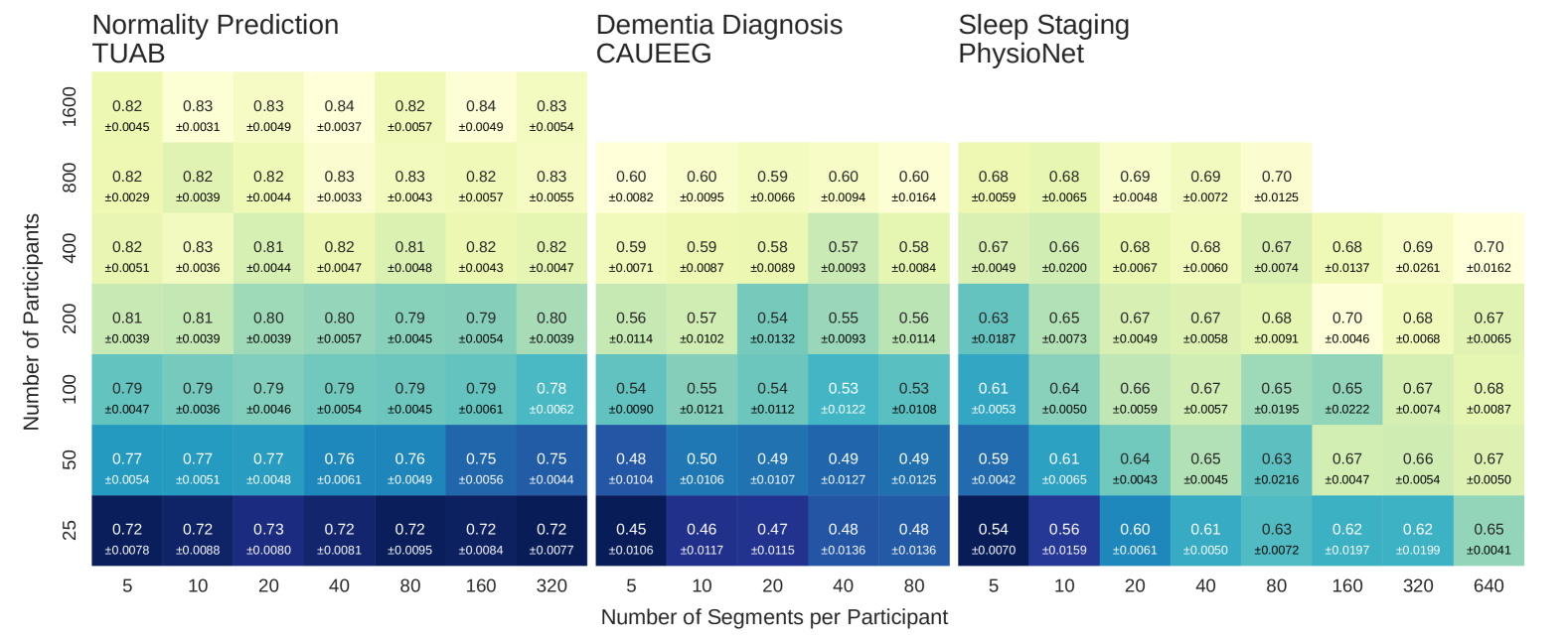
Figure 6: Baseline performance heatmap for the mAtt model. Accuracies for normality prediction on TUAB, dementia diagnosis on CAUEEG, and sleep staging on PhysioNet averaged across seeds, along with the standard error of the mean.

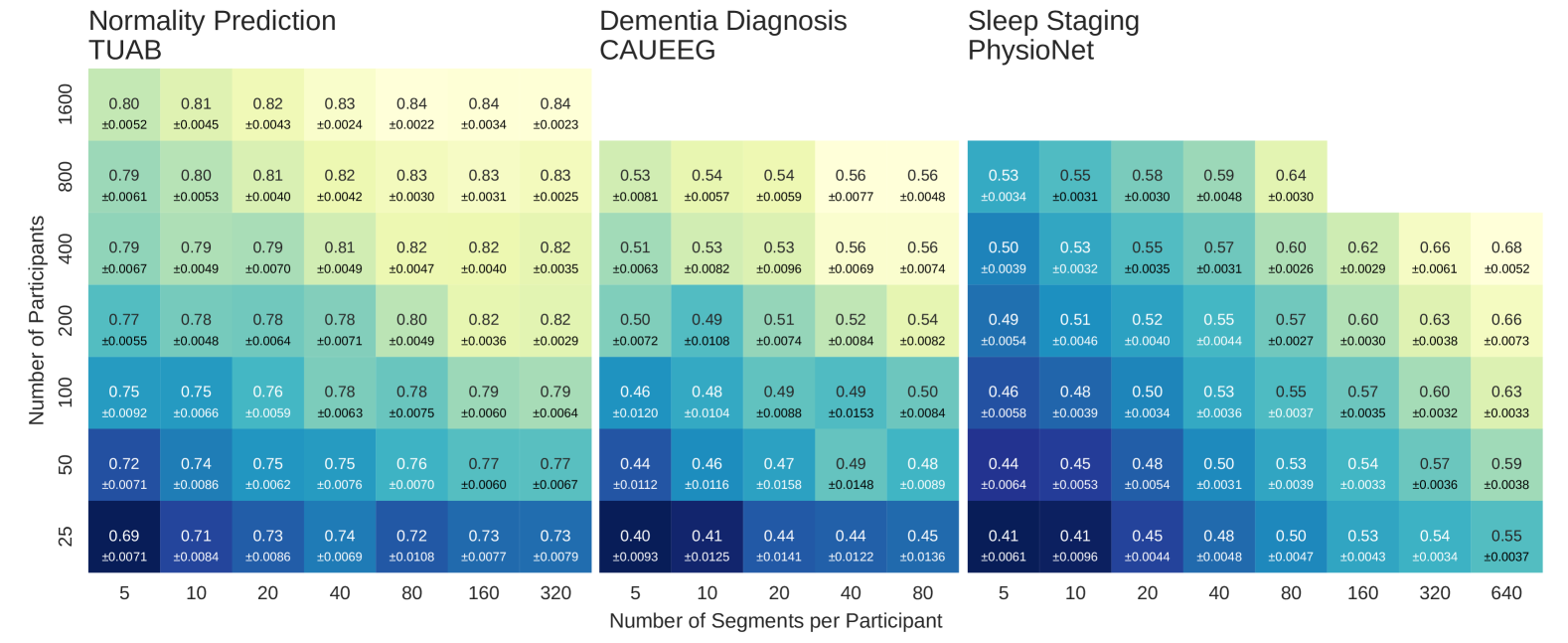
Figure 7: Baseline performance heatmap for the LaBraM model. Accuracies for normality prediction on TUAB, dementia diagnosis on CAUEEG, and sleep staging on PhysioNet averaged across seeds, along with the standard error of the mean.

A.2 Ablation: LaBraM-compatible Preprocessing

Data for the training and fine-tuning of the LaBraM model was preprocessed separately to ensure compatibility with the official pre-trained weights. On the PhysioNet dataset, this also meant that the segment length had to be reduced from 30s to 15s. Since LaBraM’s performance on PhysioNet was particularly low compared to the other models, we performed an ablation study to see how much of the performance gap should be attributed to the different preprocessing rather than to architectural differences. Specifically, we trained the TCN model using the same preprocessing that was used for the LaBraM model. Figure 8 shows that performance decreased (light blue line vs dark blue line) but was still higher than the LaBraM baseline performance (light green line). With pre-training, LaBraM achieved comparable performance to the TCN model when the same preprocessing was used (dark blue and dark green lines). Overall, this suggests that the different preprocessing explains part of the performance gap, but not all of it. When models were trained from scratch, TCN still achieved better performance.

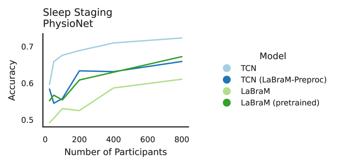
Figure 8: Ablation: LaBraM-compatible preprocessing. The light blue and dark blue lines represent TCN performance with standard and LaBraM-compatible preprocessing, respectively, while the light green and dark green lines show LaBraM performance without and with pre-training. The performance drop observed for TCN with LaBraM-compatible preprocessing suggests that preprocessing differences contributed to LaBraM’s lower baseline performance. However, the fact that TCN still outperformed LaBraM when both used the same preprocessing indicates that architectural differences also played a role. Pre-training LaBraM mitigated the performance gap, allowing it to achieve results comparable to the TCN model when both used the same preprocessing.

A.3 Pre-training Results on CAUEEG and PhysioNet

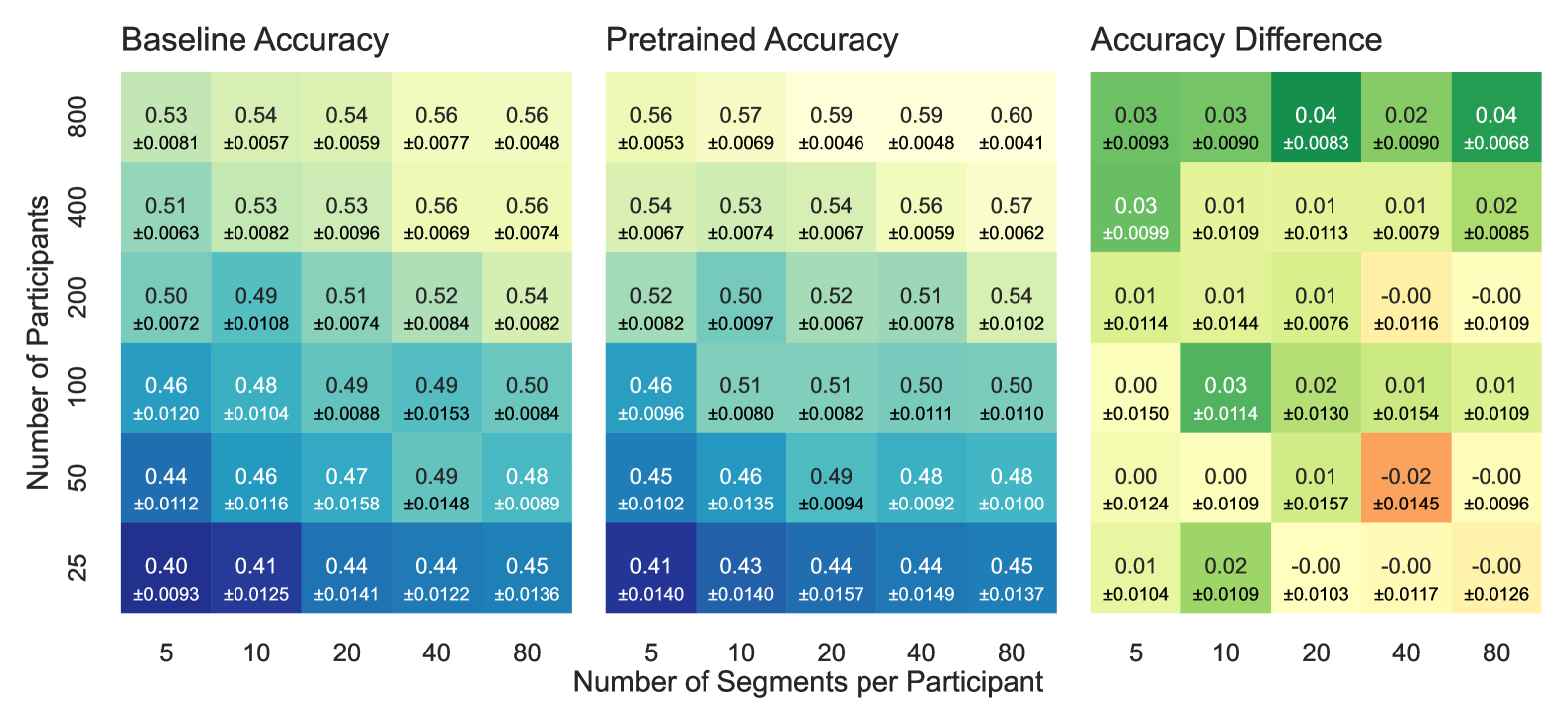
Figure 9: Effect of pre-training on the CAUEEG dataset. Comparison of LaBraM performance with and without pre-training on CAUEEG. The left and middle heatmaps show average accuracies (± standard error of the mean) for LaBraM trained from scratch (baseline) and pre-trained on a collection of 16 datasets before fine-tuning on CAUEEG, respectively. The right heatmap visualises the average of pairwise accuracy differences (± standard error of the mean), where pairs correspond to the accuracies of pre-trained and baseline models for the same seed.

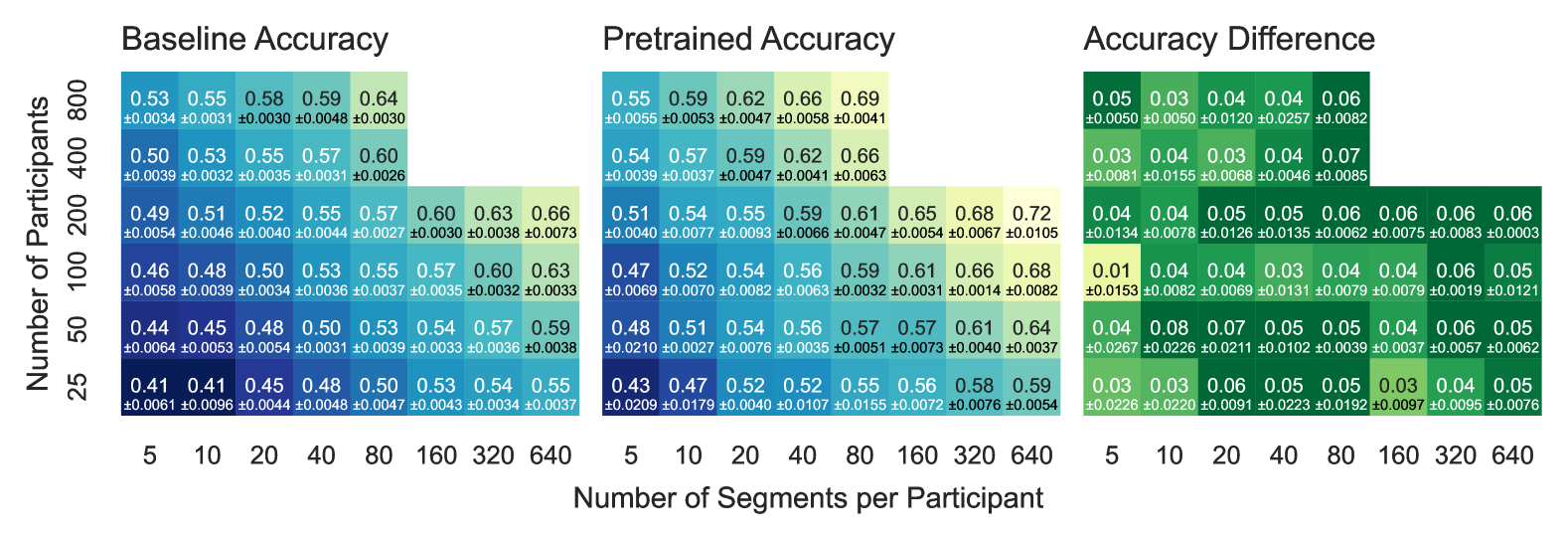
Figure 10: Effect of pre-training on the PhysioNet dataset. Comparison of LaBraM performance with and without pre-training on PhysioNet. The left and middle heatmaps show average accuracies (± standard error of the mean) for LaBraM trained from scratch (baseline) and pre-trained on a collection of 16 datasets before fine-tuning on PhysioNet, respectively. The right heatmap visualises the average of pairwise accuracy differences (± standard error of the mean), where pairs correspond to the accuracies of pre-trained and baseline models for the same seed.

A.4 Scaling Behaviour Plots with Pre-trained LaBraM Model

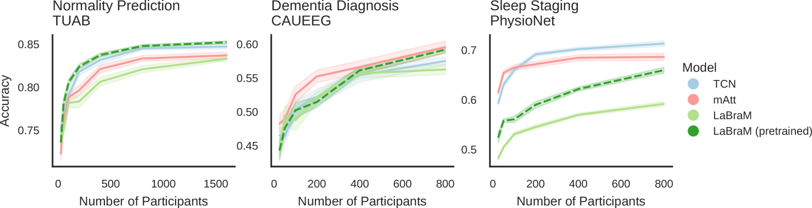
Figure 11: Scaling behaviour with pre-trained LaBraM model. Lines show the average accuracy across seeds with the standard error of the mean. Pre-training consistently improved LaBraM’s performance and allowed it to achieve comparable or even superior results to the other models. The lower performance on the PhysioNet dataset is due to differences in preprocessing (see Section A.2).

References

- [1] Lukas A.. Gemein et al. “Machine-learning-based diagnostics of EEG pathology” In NeuroImage 220, 2020, pp. 117021 DOI: 10.1016/j.neuroimage.2020.117021
- [2] Wei Wu et al. “An electroencephalographic signature predicts antidepressant response in major depression” Publisher: Nature Publishing Group In Nature Biotechnology 38.4, 2020, pp. 439–447 DOI: 10.1038/s41587-019-0397-3
- [3] Jin Jing et al. “Development of Expert-Level Classification of Seizures and Rhythmic and Periodic Patterns During EEG Interpretation” Publisher: Wolters Kluwer In Neurology 100.17, 2023, pp. e1750–e1762 DOI: 10.1212/WNL.0000000000207127
- [4] James Mitchell Crow “Could biomarkers mean better pain treatment?” Bandiera_abtest: a Cg_type: Outlook Publisher: Nature Publishing Group Subject_term: Personalized medicine, Neuroscience, Imaging, Machine learning In Nature 633.8031, 2024, pp. S28–S30 DOI: 10.1038/d41586-024-03004-1
- [5] Yannick Roy et al. “Deep learning-based electroencephalography analysis: a systematic review” In Journal of Neural Engineering 16.5, 2019, pp. 051001 DOI: 10.1088/1741-2552/ab260c
- [6] Cédric Rommel, Joseph Paillard, Thomas Moreau and Alexandre Gramfort “Data augmentation for learning predictive models on EEG: a systematic comparison” Publisher: IOP Publishing In Journal of Neural Engineering 19.6, 2022, pp. 066020 DOI: 10.1088/1741-2552/aca220
- [7] Cédric Rommel, Thomas Moreau, Joseph Paillard and Alexandre Gramfort “CADDA: Class-wise Automatic Differentiable Data Augmentation for EEG Signals” arXiv:2106.13695 [cs] arXiv, 2022 DOI: 10.48550/arXiv.2106.13695
- [8] Olawunmi George et al. “Data augmentation strategies for EEG-based motor imagery decoding” Publisher: Elsevier In Heliyon 8.8, 2022 DOI: 10.1016/j.heliyon.2022.e10240
- [9] Mostafa Neo Mohsenvand, Mohammad Rasool Izadi and Pattie Maes “Contrastive Representation Learning for Electroencephalogram Classification” Publisher: PMLR, 2020 URL: https://proceedings.mlr.press/v136/mohsenvand20a.html
- [10] Connor Shorten and Taghi M. Khoshgoftaar “A survey on Image Data Augmentation for Deep Learning” In Journal of Big Data 6.1, 2019, pp. 60 DOI: 10.1186/s40537-019-0197-0
- [11] Linus Ericsson, Henry Gouk, Chen Change Loy and Timothy M. Hospedales “Self-Supervised Representation Learning: Introduction, advances, and challenges” Conference Name: IEEE Signal Processing Magazine In IEEE Signal Processing Magazine 39.3, 2022, pp. 42–62 DOI: 10.1109/MSP.2021.3134634
- [12] Hsiang-Yun Sherry Chien, Hanlin Goh, Christopher M. Sandino and Joseph Y. Cheng “MAEEG: Masked Auto-encoder for EEG Representation Learning” arXiv:2211.02625 [cs, eess] arXiv, 2022 URL: http://arxiv.org/abs/2211.02625
- [13] Wenhui Cui et al. “Neuro-GPT: Developing A Foundation Model for EEG” In arXiv, 2023 URL: https://arxiv.org/abs/2311.03764
- [14] Wei-Bang Jiang, Li-Ming Zhao and Bao-Liang Lu “Large Brain Model for Learning Generic Representations with Tremendous EEG Data in BCI”, 2023 URL: https://openreview.net/forum?id=QzTpTRVtrP
- [15] Yonghao Song, Qingqing Zheng, Bingchuan Liu and Xiaorong Gao “EEG conformer: convolutional transformer for EEG decoding and visualization.” In IEEE Transactions on Neural Systems and Rehabilitation Engineering PP, 2022 DOI: 10.1109/TNSRE.2022.3230250
- [16] Rishi Bommasani et al. “On the Opportunities and Risks of Foundation Models” arXiv:2108.07258 [cs] arXiv, 2022 DOI: 10.48550/arXiv.2108.07258
- [17] Steve Hanneke, Kasper Green Larsen and Nikita Zhivotovskiy “Revisiting Agnostic PAC Learning” arXiv:2407.19777 [cs, math, stat] arXiv, 2024 DOI: 10.48550/arXiv.2407.19777
- [18] Steve Hanneke “The Optimal Sample Complexity of PAC Learning” In Journal of Machine Learning Research 17.38, 2016, pp. 1–15 URL: http://jmlr.org/papers/v17/15-389.html
- [19] Henry Gouk, Ondrej Bohdal, Da Li and Timothy Hospedales “On the Limitations of General Purpose Domain Generalisation Methods” arXiv:2202.00563 arXiv, 2024 DOI: 10.48550/arXiv.2202.00563
- [20] Ira R.. Hebold Haraldsen et al. “AI-Mind: Revolutionizing Personalized Neurology Through Automated Diagnostics and Advanced Data Management” Publisher: ScienceOpen In Drug Repurposing 1, 2024, pp. 20240005 DOI: 10.58647/DRUGREPO.24.1.0005
- [21] Jared Kaplan et al. “Scaling Laws for Neural Language Models” arXiv:2001.08361 arXiv, 2020 DOI: 10.48550/arXiv.2001.08361
- [22] Linus Ericsson, Henry Gouk and Timothy M. Hospedales “Why Do Self-Supervised Models Transfer? Investigating the Impact of Invariance on Downstream Tasks” In British Machine Vision Conference (BMVC), 2022
- [23] Ranjan Debnath et al. “The Maryland analysis of developmental EEG (MADE) pipeline” In Psychophysiology 57.6, 2020, pp. e13580 DOI: 10.1111/psyp.13580
- [24] Mainak Jas et al. “Autoreject: Automated artifact rejection for MEG and EEG data” In NeuroImage 159, 2017, pp. 417–429 DOI: 10.1016/j.neuroimage.2017.06.030
- [25] Luca Pion-Tonachini, Ken Kreutz-Delgado and Scott Makeig “ICLabel: An automated electroencephalographic independent component classifier, dataset, and website” In NeuroImage 198, 2019, pp. 181 DOI: 10.1016/j.neuroimage.2019.05.026
- [26] Anders Gjølbye et al. “SPEED: Scalable Preprocessing of EEG Data for Self-Supervised Learning” arXiv:2408.08065 [eess] arXiv, 2024 DOI: 10.48550/arXiv.2408.08065
- [27] Philipp Bomatter et al. “Machine learning of brain-specific biomarkers from EEG” Publisher: Elsevier In eBioMedicine 106, 2024 DOI: 10.1016/j.ebiom.2024.105259
- [28] Alexandra L. Young et al. “Uncovering the heterogeneity and temporal complexity of neurodegenerative diseases with Subtype and Stage Inference” Publisher: Nature Publishing Group In Nature Communications 9.1, 2018, pp. 4273 DOI: 10.1038/s41467-018-05892-0
- [29] Amanda M. Buch and Conor Liston “Dissecting diagnostic heterogeneity in depression by integrating neuroimaging and genetics” Publisher: Nature Publishing Group In Neuropsychopharmacology 46.1, 2021, pp. 156–175 DOI: 10.1038/s41386-020-00789-3
- [30] S. López et al. “Automated Identification of Abnormal Adult EEGs” In … IEEE Signal Processing in Medicine and Biology Symposium (SPMB). IEEE Signal Processing in Medicine and Biology Symposium 2015, 2015 DOI: 10.1109/SPMB.2015.7405423
- [31] Lopez de Diego and Silvia Isabel “Automated Interpretation of Abnormal Adult Electroencephalograms” Accepted: 2020-10-27T15:14:14Z Publisher: Temple University. Libraries, 2017 URL: https://scholarshare.temple.edu/handle/20.500.12613/1767
- [32] Iyad Obeid and Joseph Picone “The Temple University Hospital EEG Data Corpus” Publisher: Frontiers In Frontiers in Neuroscience 10, 2016 DOI: 10.3389/fnins.2016.00196
- [33] Devon I. Rubin “Clinical Neurophysiology”, Contemporary Neurology Ser Oxford: Oxford University Press USA - OSO, 2021
- [34] Min-jae Kim, Young Chul Youn and Joonki Paik “Deep learning-based EEG analysis to classify normal, mild cognitive impairment, and dementia: Algorithms and dataset” In NeuroImage 272, 2023, pp. 120054 DOI: 10.1016/j.neuroimage.2023.120054
- [35] Mohammad M. Ghassemi et al. “You Snooze, You Win: the PhysioNet/Computing in Cardiology Challenge 2018” In Computing in cardiology 45, 2019, pp. 10.22489/cinc.2018.049 DOI: 10.22489/cinc.2018.049
- [36] A.. Goldberger et al. “PhysioBank, PhysioToolkit, and PhysioNet: components of a new research resource for complex physiologic signals” In Circulation 101.23, 2000, pp. E215–220 DOI: 10.1161/01.cir.101.23.e215
- [37] Shaojie Bai, J. Kolter and Vladlen Koltun “An Empirical Evaluation of Generic Convolutional and Recurrent Networks for Sequence Modeling” arXiv:1803.01271 [cs] arXiv, 2018 DOI: 10.48550/arXiv.1803.01271
- [38] Robin Tibor Schirrmeister et al. “Deep learning with convolutional neural networks for EEG decoding and visualization” _eprint: https://onlinelibrary.wiley.com/doi/pdf/10.1002/hbm.23730 In Human Brain Mapping 38.11, 2017, pp. 5391–5420 DOI: 10.1002/hbm.23730
- [39] Yue-Ting Pan, Jing-Lun Chou and Chun-Shu Wei “MAtt: A Manifold Attention Network for EEG Decoding” In Advances in Neural Information Processing Systems 35, 2022, pp. 31116–31129 URL: https://papers.nips.cc/paper_files/paper/2022/hash/c981fd12b1d5703f19bd8289da9fc996-Abstract-Conference.html
- [40] H Aurlien et al. “EEG background activity described by a large computerized database” In Clinical Neurophysiology 115.3, 2004, pp. 665–673 DOI: 10.1016/j.clinph.2003.10.019
- [41] A… Chiang et al. “Age trends and sex differences of alpha rhythms including split alpha peaks” In Clinical Neurophysiology 122.8, 2011, pp. 1505–1517 DOI: 10.1016/j.clinph.2011.01.040
- [42] Dillan Cellier, Justin Riddle, Isaac Petersen and Kai Hwang “The development of theta and alpha neural oscillations from ages 3 to 24 years” In Developmental Cognitive Neuroscience 50, 2021, pp. 100969 DOI: 10.1016/j.dcn.2021.100969
- [43] Justus T.. Schwabedal et al. “Addressing Class Imbalance in Classification Problems of Noisy Signals by using Fourier Transform Surrogates” arXiv:1806.08675 [nlin, q-bio, stat] arXiv, 2019 DOI: 10.48550/arXiv.1806.08675
- [44] Robert J. Thomas, Sushanth Bhat and Sudhansu Chokroverty “Atlas of Sleep Medicine” Cham: Springer, 2023