On the formation of the $1:2$ resonance in oscillator dynamics

Abstract

The dynamics of nonlinear oscillators are investigated. We study the formation of $1:2$ resonance in nonlinear periodically forced oscillators due to period doubling of the primary $1:1$ resonance, or born independently. We compute the amplitude-frequency implicit function, the steady-state asymptotic solution, for the effective equation approximating coupled oscillators. Working in the framework of differential properties of implicit functions, we demonstrate that birth of $1:2$ resonances corresponds to singular isolated points of the implicit functions. We provide numerical examples illustrating our theoretical findings.

1 Introduction

Recently, we have investigated metamorphoses of $1:2$ resonance and its interaction with the primary resonance in the asymmetric Duffing oscillator [1]. The study documented very complicated dynamics of the $1:2$ resonance. This work studies the $1:2$ resonance formation in nonlinear periodically forced oscillators. The $1:2$ resonance is due to period doubling of the main $1:1$ resonance or is born independently. The latter phenomenon has not yet been investigated and deserves a separate study.

We consider an effective equation describing approximately the dynamics of coupled oscillators, and its special case, the Duffing equation.

Coupled oscillators can model dynamics encountered in mechanics, chemistry, electronics, and neuroscience, see [2, 3, 4, 5, 6, 7, 8, 9, 10, 11, 12, 13, 14, 15] and references therein. A generic example is a dynamic vibration absorber, consisting of a mass $m_{2}$, attached to the main vibrating system of mass $m_{1}$ [16, 17] and governed by equations

$$\left.\begin{array}[]{l}m_{1}\ddot{x}_{1}-V_{1}\left(\dot{x}_{1}\right)-R_{1}\left(x_{1}\right)+V_{2}\left(\dot{x}_{2}-\dot{x}_{1}\right)+R_{2}\left(x_{2}-x_{1}\right)=f\cos\left(\omega t\right)\\ m_{2}\ddot{x}_{2}-V_{2}\left(\dot{x}_{2}-\dot{x}_{1}\right)-R_{2}\left(x_{2}-x_{1}\right)=0\end{array}\right\}$$ (1)

where $V_{1}$, $R_{1}$ and $V_{2}$, $R_{2}$ are (nonlinear) force of internal friction and (nonlinear) elastic restoring force for mass $m_{1}$ and mass $m_{2}$, respectively.

2 Approximate effective equation and the Duffing equation

In what follows we make a simplifying assumption

$$R_{1}\left(x_{1}\right)=-\alpha_{1}x_{1},\ V_{1}\left(\dot{x}_{1}\right)=-\nu_{1}\dot{x}_{1}.$$ (2)

Now, in new variables, $x\equiv x_{1}$, $y\equiv x_{2}-x_{1}$, we eliminate variable $x$ to obtain the following exact equation for relative motion [18, 19]

$$\left(M\tfrac{d^{2}}{dt^{2}}+\nu\tfrac{d}{dt}+\alpha\right)\left(\mu\ddot{y}-V_{e}\left(\dot{y}\right)-R_{e}\left(y\right)\right)+\epsilon m_{e}\left(\nu\tfrac{d}{dt}+\alpha\right)\ddot{y}=F\cos\left(\omega t\right),$$ (3)

where $m\equiv m_{1}$, $m_{e}\equiv m_{2}$, $\nu=\nu_{1}$, $\alpha=\alpha_{1}$, $M=m+m_{e}$, $F=m_{e}\omega^{2}f$, $\mu=mm_{e}/M$, $\epsilon=m_{e}/M$ and $R_{e}\equiv R_{2}$, $V_{e}\equiv V_{2}$.

In the present work, we put

$$R_{e}\left(y\right)=\alpha_{e}y-\gamma_{e}y^{3},\quad V_{e}\left(\dot{y}\right)=-\nu_{e}\dot{y},$$ (4)

and assume that $\epsilon m_{e}$, $\nu$, $\alpha$ are small, and, accordingly, the term proportional to $\epsilon m_{e}$ can be neglected.

Introducing nondimensional time $\tau$ and rescaling variable $y$

$$\tau=t\bar{\omega},\ \bar{\omega}=\sqrt{\frac{\alpha_{e}}{\mu}},\ z=y\sqrt{\frac{\gamma_{e}}{\alpha_{e}}},$$ (5)

we get the approximate effective equation [18]

$$\frac{d^{2}z}{d\tau^{2}}+h\frac{dz}{d\tau}-z+z^{3}=-\gamma\frac{\Omega^{2}}{\sqrt{\left(\Omega^{2}-a\right)^{2}+H^{2}\Omega^{2}}}\cos\left(\Omega\tau+\delta\right),$$ (6)

where $\gamma\equiv G\dfrac{\kappa}{\kappa+1}$, $\tan\delta=\frac{\omega\nu}{M\left(\omega^{2}-\omega_{0}^{2}\right)}=\frac{H\Omega}{\Omega^{2}-\Omega_{0}^{2}}=\frac{H\Omega}{\Omega^{2}-a}$, and where nondimensional quantities are given by

$$\left.\begin{array}[]{l}h=\frac{\nu_{e}}{\mu\bar{\omega}}\text{,}\ H=\frac{\nu}{M\bar{\omega}}\text{,}\ \Omega=\frac{\omega}{\bar{\omega}}\text{,}\ \Omega_{0}=\frac{\omega_{0}}{\bar{\omega}}\text{,}\ \omega_{0}=\sqrt{\frac{\alpha}{M}}\text{, }\\ G=\frac{1}{\alpha_{e}}\sqrt{\frac{\gamma_{e}}{\alpha_{e}}}f\text{,}\ \kappa=\frac{m_{e}}{m}\text{,}\ a=\frac{\alpha\mu}{\alpha_{e}M}\text{.}\end{array}\right\}$$ (7)

For $a=H=0$ Eq. (6) reduces to the Duffing equation with $\delta=0$

$$\frac{d^{2}z}{d\tau^{2}}+h\frac{dz}{d\tau}-z+z^{3}=-\gamma\cos\left(\Omega\tau\right).$$ (8)

3 Asymptotic solution of Eq. (6) for the $1:2$ resonance

We applied the Krylov-Bogoliubov-Mitropolsky (KBM) perturbation approach [20] to the rescaled effective equation (6) proceeding as in [21, 22], obtaining for the $1:2$ resonance of form

$$z\left(\tau\right)=A_{0}+A\cos\left(\tfrac{1}{2}\Omega\tau+\tfrac{1}{2}\delta+\varphi\right)$$ (9)

the following solution

$$\tfrac{3}{2}A_{0}A^{2}+A_{0}^{3}+\tfrac{3}{2}A_{0}C^{2}-A_{0}+\tfrac{3}{4}CA^{2}\cos\left(2\varphi-\delta\right) = 0$$ (10a)

$$\tfrac{1}{2}hA\Omega-3A_{0}CA\sin\left(2\varphi-\delta\right) = 0$$ (10b)

$$\tfrac{1}{4}A\Omega^{2}+A-3A_{0}^{2}A-\tfrac{3}{2}C^{2}A-\tfrac{3}{4}A^{3}-3A_{0}CA\cos\left(2\varphi-\delta\right) = 0$$ (10c)

where (we assume that the denominators do not vanish)

$$C=-\gamma\dfrac{\Omega^{2}}{\sqrt{\left(\Omega^{2}-a\right)^{2}+H^{2}\Omega^{2}}}\dfrac{1}{\frac{3}{4}A^{2}-\Omega^{2}-1}$$ (10d)

We eliminate the phase $2\varphi-\delta$ and compute $A_{0}^{2}$ obtaining the following, rather complicated, implicit function $F$ of variables $\Omega,\ A$ and parameters $h$, $a$, $H$, $\gamma$ (assuming that the denominators do not vanish)

$$\left.\begin{array}[]{l}F\left(\Omega,A;h,a,H,\gamma\right)=A_{0}^{4}+c_{2}A_{0}^{2}+c_{0}=0\vskip 6.0pt plus 2.0pt minus 2.0pt\\ c_{2}=\tfrac{3}{4}A^{2}+\tfrac{3}{2}C^{2}-1,\ c_{0}=-\tfrac{3}{16}A^{4}+\left(\tfrac{1}{16}\Omega^{2}-\tfrac{3}{8}C^{2}+\tfrac{1}{4}\right)A^{2}\vskip 3.0pt plus 1.0pt minus 1.0pt\\ A_{0}^{2}=\frac{\Omega^{4}+\left(8-15A^{2}+4h^{2}-12C^{2}\right)\Omega^{2}+6C^{2}\left(6C^{2}-8+15A^{2}\right)+4\left(3A^{2}-4\right)\left(3A^{2}-1\right)}{12\left(2\Omega^{2}+3A^{2}+18C^{2}-4\right)}\vskip 3.0pt plus 1.0pt minus 1.0pt\\ C=-\gamma\frac{\Omega^{2}}{\sqrt{\left(\Omega^{2}-a\right)^{2}+H^{2}\Omega^{2}}}\frac{1}{\frac{3}{4}A^{2}-\Omega^{2}-1}\end{array}\right\}$$ (11)

4 Singular points of implicit function (11)

Singular points of the implicit function $F\left(\Omega,A;h,a,H,\gamma\right)=0$ are given by [23, 24]

$$F\left(\Omega,A;h,a,H,\gamma\right) = 0$$ (12a)

$$\frac{\partial F\left(\Omega,A;h,a,H,\gamma\right)}{\partial A} = 0$$ (12b)

$$\frac{\partial F\left(\Omega,A;h,a,H,\gamma\right)}{\partial\Omega} = 0$$ (12c)

If we assume, for example, values of $h$, $a$, and $H$, we can solve Eqs. (12) for $\Omega$, $A$, $\gamma$ numerically.

We can also consider a special case of singular points with $A=0$. The corresponding conditions read

$$F\left(\Omega,0;h,a,H,\gamma\right) = 0$$ (13a)

$$\frac{\partial F\left(\Omega,0;h,a,H,\gamma\right)}{\partial\Omega} = 0$$ (13b)

since $\left.\dfrac{\partial F\left(\Omega,A;h,a,H,\gamma\right)}{\partial A}\right|_{A=0}\equiv 0$.

Equations (13) can be solved for $h,\ \gamma$ yielding two polynomial equations with coefficients depending on $\Omega$, $a$, $H$, see Appendix A. Alternatively, we assume values of $\Omega$, $a$, $H$, solve Eqs. (13) numerically and choose physical solutions $(h>0$, $\gamma$ – real$)$.

In the case of the Duffing equation, $a=H=0$, equations (13) (or (A.1), (A.2)) can be simplified significantly

$$f\left(\Omega,h\right)=27\Omega^{8}+\left(252h^{2}-486\right)\Omega^{6}+\left(2259-2400h^{2}+500h^{4}\right)\Omega^{4}$$ (14a)

$$+\left(1224+2484h^{2}+200h^{4}\right)\Omega^{2}+20h^{4}-624h^{2}-16\,128=0\vskip 3.0pt plus 1.0pt minus 1.0pt$$

$$\hskip-50.0ptg\left(\Omega,h,\gamma\right)=\left(69h^{2}-126\right)\Omega^{6}+\left(230h^{4}-1368h^{2}+1197\right)\Omega^{4}$$ (14b)

$$+\left(76h^{4}+789h^{2}-387\right)\Omega^{2}+6h^{4}-654h^{2}-9000+\left(828h^{2}+108\right)\gamma^{2}=0$$

We are mainly interested in singular points which are isolated points of the implicit function $F\left(\Omega,A;h,a,H,\gamma\right)=0$. This is because isolated points with $A\neq 0$ are solutions of Eqs. (12), correspond to the birth of the $1:2$ resonance (in all investigated cases out of chaos), while singular points with $A=0$, solutions of Eqs. (13), correspond to the birth of the $1:2$ resonance due to period doubling of the main $1:1$ resonance.

5 Examples of birth of $1:2$ resonances

5.1 The Duffing equation

To study the Duffing equation (8) we put $a=H=0$ in equations (12), (13). Moreover, we assume, arbitrarily, $h=0.7$.

Equation (14a), $f\left(\Omega,0.7\right)=0$, has only two real roots, $\Omega=\pm 2.\,617\,420$. Then the equation (14b), $g\left(2.\,617\,420,0.7,\gamma\right)=0$, yields $\gamma=\pm 4.\,737\,197$. Therefore, for $h=0.7$, $\gamma=4.\,737\,197$ the singular point of the Duffing implicit function $F\left(\Omega,A;h,0,0,\gamma\right)=0$ arises – this is an isolated point $\left(\Omega,A\right)=\left(2.\,617\,420,0\right)$.

We now solve numerically Eqs. (12) for $h=0.7$, $a=0$, $H=0$. We obtain, of course, the previous solution, and $\left(\Omega,A_{\pm}\right)=\left(1.\,358\,480,\pm 0.813\,037\right)$ for $\gamma=2.\,168\,300$.

All computed singular points are isolated points and are shown in the plot below; see red dots in figure 1.

For decreasing $\gamma$, the first singular point appears at $\gamma=4.\,737\,197$. In this isolated point $A=0$ and, therefore, corresponds to first period doubling of the main $1:1$ resonance.

Then, at $\gamma=2.\,168\,300$ a pair of singular isolated points is created, $\Omega=1.\,358\,480$, $A_{\pm}=\pm 0.813\,037$. Since $A\neq 0$, these isolated points correspond to birth of two branches of $1:2$ resonance, without a contact with the main resonance.

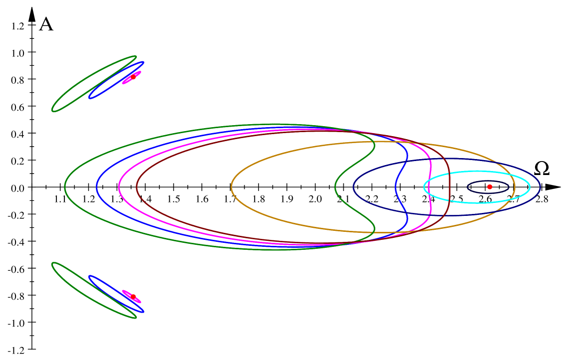
Figure 1: Sequential metamorphoses of amplitude-frequency implicit function $F\left(\Omega,A;h,0,0,\gamma\right)=0$, describing $1:2$ resonance; $\gamma=2.15$ (Magenta), $\gamma=2.274$ (Red), $\gamma=3$ (Sienna), $\gamma=4$ (Blue), $\gamma=4.5$ (LtBlueGreen), $\gamma=4.7$ (Navy).

To demonstrate the role of the singular points, we have computed bifurcation diagrams for $h=0.7$ and variable $\gamma$.

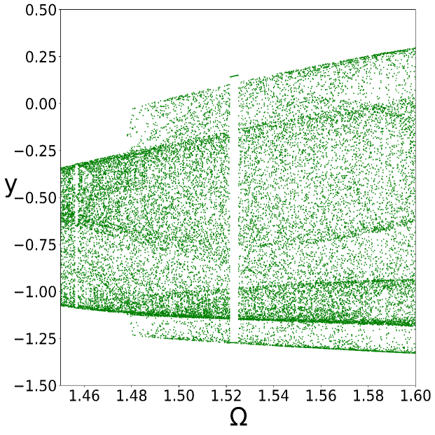
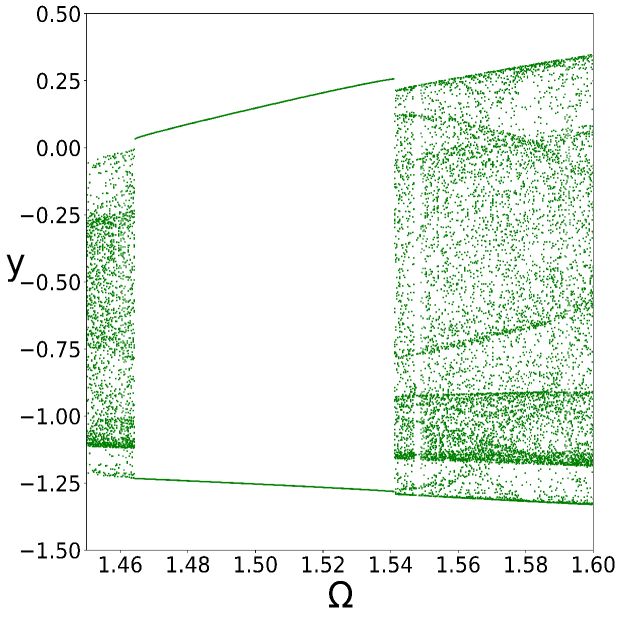
Figure 2: Bifurcation diagrams: $\gamma=1.9978$ – left figure, $\gamma=1.95$ – right figure.

Left-hand figure 2 shows birth of $1:2$ resonance out from chaos. Right-hand figure 2 displays a fully developed $1:2$ resonance. The resonance appears at $\gamma=1.9978$, in qualitative agreement with the computed value $\gamma=2.\,168\,300$.

Fig. 3 describes period doubling of $1:1$ resonance. Red curve corresponds to the $1:1$ resonance just before the first period doubling at $\gamma>4.21$. Green and blue curves show growth of the $1:2$ resonance (before the next period doubling).

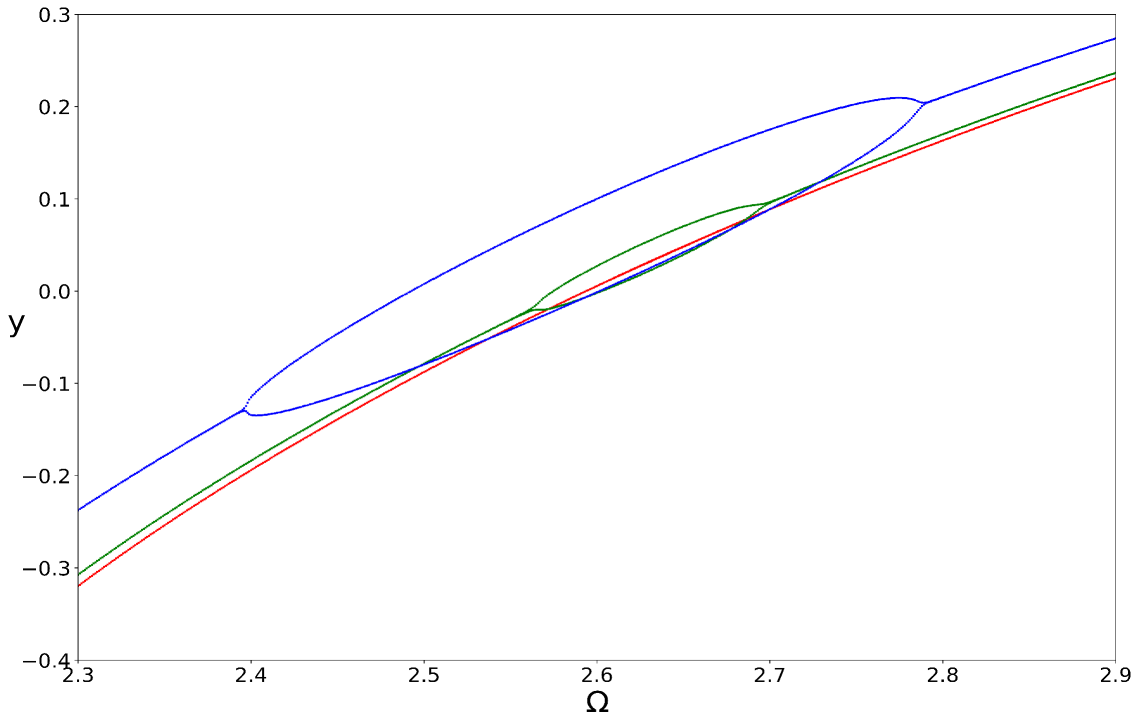
Figure 3: Bifurcation diagram, $\gamma=4.21$ – Red, $\gamma=4.18$ – Green, $\gamma=4.00$ – Blue.

5.2 The effective equation

We consider an effective equation with, for example, $a=-0.8$, $H=0.5$, and assume, as before, $h=0.7$.

We now solve Eqs. (12) numerically, obtaining several solutions. Namely, we get $\gamma=3.\,159\,196$ and $\left(\Omega,A\right)=\left(1.\,001\,811,\pm 0.527\,685\right)$ – self-intersections, as well as $\gamma=3.\,\allowbreak 243\,191$ and $\left(\Omega,A\right)=\left(1.\,295\,330,\pm 0.742\,884\right)$ – a pair of isolated points.

We solve Eqs. (13) numerically, obtaining again several solutions. There is a solution $\gamma=5.\,375\,442$, $\left(\Omega,A\right)=\left(2.\,581\,157,0\right)$, corresponding to an isolated point. Figure below shows all singular points (red dots).

The first singular point appears, for decreasing $\gamma$, at $\gamma=5.\,375\,442$. In this isolated point $A=0$ and, therefore, corresponds to the first period doubling of the main $1:1$ resonance.

Then, at $\gamma=3.\,\allowbreak 243\,191$ a pair of singular isolated points is created, $\Omega=1.\,295\,330$, $A_{\pm}=\pm 0.742\,884$. Since $A\neq 0$, these isolated points correspond to birth of two branches of $1:2$ resonance, without a contact with the main resonance.

There is also a pair of self-intersections for $\gamma=3.\,159\,196$, unrelated, however, to the birth of $1:2$ resonance.

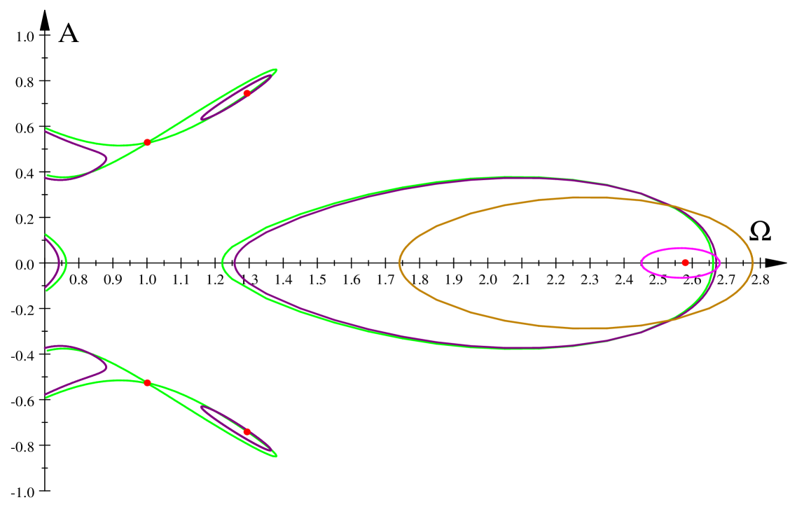
Figure 4: Amplitude-frequency implicit function $F\left(\Omega,A;h,a,H,\gamma\right)=0$: $\gamma=5.3$ (Magenta), $\gamma=4$ (Sienna), $\gamma=3.20$ (Purple), $\gamma=3.159$ (LightGreen).

We have computed bifurcation diagrams for $a=-0.8$, $H=0.5$, $h=0.7$ and variable $\gamma$ to study if knowledge of singular points permits prediction of emergence of $1:2$ resonances.

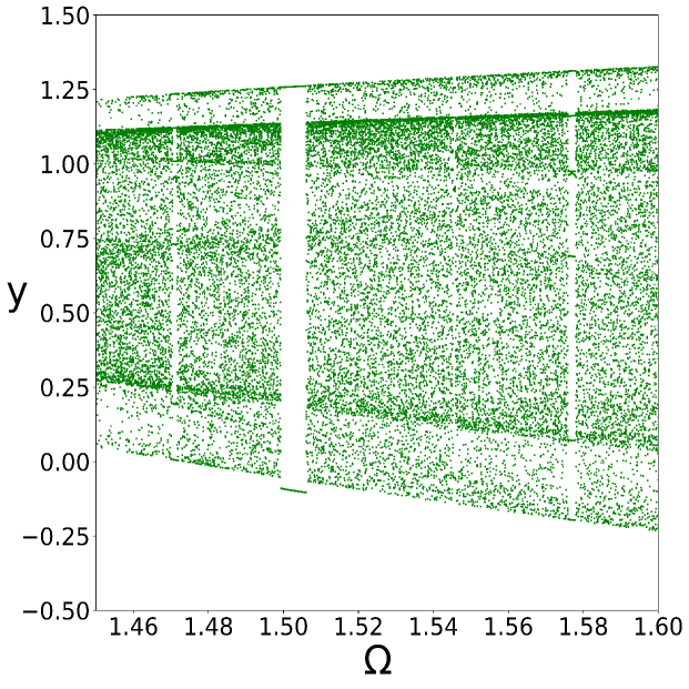
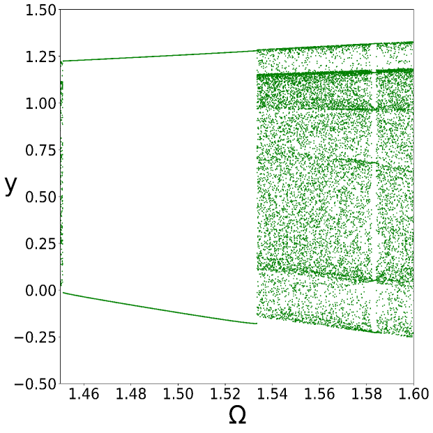
Figure 5: Bifurcation diagrams: $\gamma=2.773\,6$ – left figure, $\gamma=2.75$ – right figure.

Left-hand figure 5 shows birth of $1:2$ resonance out from chaos. Right-hand figure 5 displays a fully developed $1:2$ resonance. The resonance appears at $\gamma=4.75$, in qualitative agreement with the computed value $\gamma=5.\,375\,442$.

Fig. 6 describes period doubling of $1:1$ resonance. Red curve corresponds to the $1:1$ resonance just before the first period doubling at $\gamma>4.751$. Green and blue curves show growth of the $1:2$ resonance (before the next period doubling).

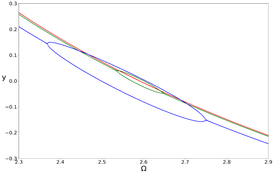
Figure 6: Bifurcation diagram, $\gamma=4.75$ – Red, $\gamma=4.77$ – Green, $\gamma=4.60$ – Blue.

6 Conclusions

We have demonstrated that on the basis of asymptotic solution(10) to the effective equation (6) (Duffing equation is a special case) the birth of $1:2$ resonances can be predicted.

More precisely, implicit function 11, computed from Eqs. (10), has singular isolated points – fulfilling Eqs. (12) – corresponding to the birth of $1:2$ resonances. Singular isolated points are computed as follows: 1. values of $h$, $a$, $H$ are chosen, 2. equations (12) are solved numerically yielding many solutions – values of $\Omega$, $A$, $\gamma$, 3. real positive solutions are selected, 4. isolated points are found – in such points $\frac{\partial^{2}F}{\partial\Omega^{2}}\frac{\partial^{2}F}{\partial A^{2}}-\left(\frac{\partial^{2}F}{\partial\Omega\partial A}\right)^{2}>0$.

There are two kinds of such singular isolated points, (i) with $A\neq 0$, (ii) with $A=0$, which are solutions of simpler equations (13) which can be simplified further; see Eqs. (A.1), (A.2). Singular isolated points of the first kind ($A\neq 0$) correspond to birth of $1:2$ resonance without contact with the primary $1:1$ resonance. Interestingly, $1:2$ resonance appears in the chaotic regime. On the other hand, singular points of the second kind ($A=0$) represent emergence of $1:2$ resonance due to period doubling of the primary resonance.

Singular isolated points computed from Eqs. (12) are very helpful in the search for the birth of $1:2$ resonances when solving Eq. 6 numerically, although the agreement is only qualitative (it can be improved upon adding in Eq. (9) the second harmonic).

Since the effective equation (6) approximates well the system of coupled oscillators [18], we expect that our findings apply also to the general model (1).

Appendix A Simplifying equations (13)

Equations (13), involving a complicated function $F\left(\Omega,0;h,a,H,\gamma\right)$, can be simplified. More precisely, they can be reduced to polynomial equations (A.1), (A.2)

$$p\left(x,\Omega,a,H\right)=a_{4}\left(\Omega,a,H\right)x^{4}+a_{2}\left(\Omega,a,H\right)x^{2}+a_{0}\left(\Omega,a,H\right)=0$$ (A.1)

where $x=\gamma\frac{\Omega^{2}}{1+\Omega^{2}}$ and coefficients $a_{4}$, $a_{2}$, and $a_{0}$ are given below

$a_{4}\left(\Omega,a,H\right)=\sum\nolimits_{k=0}^{3}c_{k}\Omega^{2k}$
$c_{3}=1800$
$c_{2}=-2160a+360+1080H^{2}$
$c_{1}=-360H^{2}+720a+360a^{2}$
$c_{0}=-360H^{2}+720a+360a^{2}$

$a_{2}\left(\Omega,a,H\right)=\sum\nolimits_{k=0}^{6}c_{k}\Omega^{2k}$
$c_{6}=48$
$c_{5}=72H^{2}-1008-144a$
$c_{4}=144a^{2}+3408a+24H^{4}-96aH^{2}-1704H^{2}-336$
$c_{3}=2784aH^{2}-336H^{2}+672a+24a^{2}H^{2}-48a^{3}-696H^{4}-4176a^{2}$
$c_{2}=-1080a^{2}H^{2}+2160a^{3}$
$c_{1}=-672a^{3}-384a^{4}+336a^{2}H^{2}$
$c_{0}=336a^{4}$

$a_{0}\left(\Omega,a,H\right)=\sum\nolimits_{k=0}^{9}c_{k}\Omega^{2k}$
$c_{9}=-1$
$c_{8}=-1+6a-3H^{2}$
$c_{7}=-15a^{2}+6a-3H^{2}-3H^{4}+64+12aH^{2}$
$c_{6}=\left(\begin{array}[]{l}-15a^{2}-18a^{2}H^{2}+6H^{4}a+192H^{2}+64\\ +20a^{3}+12aH^{2}-384a-H^{6}-3H^{4}\end{array}\right)$
$c_{5}=\left(\begin{array}[]{l}-15a^{4}-384a+192H^{2}-18a^{2}H^{2}+20a^{3}+6H^{4}a\\ -768aH^{2}-H^{6}+192H^{4}+12a^{3}H^{2}-3a^{2}H^{4}+960a^{2}\end{array}\right)$
$c_{4}=\left(\begin{array}[]{l}-3a^{4}H^{2}-3a^{2}H^{4}+192H^{4}-768aH^{2}+64H^{6}+1152a^{2}H^{2}\\ +6a^{5}+12a^{3}H^{2}-15a^{4}-1280a^{3}+960a^{2}-384H^{4}a\end{array}\right)$
$c_{3}=\left(\begin{array}[]{l}64H^{6}+1152a^{2}H^{2}-384H^{4}a+6a^{5}-768a^{3}H^{2}+192a^{2}H^{4}\\ -1280a^{3}-3a^{4}H^{2}-a^{6}+960a^{4}\end{array}\right)$
$c_{2}=-a^{6}-384a^{5}+960a^{4}+192a^{2}H^{4}-768a^{3}H^{2}+192a^{4}H^{2}$
$c_{1}=-384a^{5}+192a^{4}H^{2}+64a^{6}$
$c_{0}=64a^{6}\allowbreak$

$$q\left(y,x,\Omega,a,H\right)=b_{2}\left(\Omega,a,H\right)y^{2}+b_{0}\left(x,\Omega,a,H\right)$$ (A.2)

where $y=h\Omega$, $x=\gamma\frac{\Omega^{2}}{1+\Omega^{2}}$ is a solution of Eq. (A.1), and coefficients $b_{2}$, $b_{0}$ are provided below

$b_{2}\left(\Omega,a,H\right)=\sum\nolimits_{k=0}^{5}c_{k}\Omega^{2k}$
$c_{5}=10$
$c_{4}=-32a+16H^{2}+2$
$c_{3}=6H^{4}-24aH^{2}+36a^{2}$
$c_{2}=-16a^{3}+8aH^{2}+8a^{2}H^{2}-12a^{2}-2H^{4}$
$c_{1}=2a^{4}+16a^{3}-8a^{2}H^{2}$
$c_{0}=-6a^{4}$

$b_{0}\left(x,\Omega,a,H\right)=\sum\nolimits_{k=0}^{7}c_{k}\Omega^{2k}$
$c_{7}=3$
$c_{6}=-10a-39+5H^{2}$
$c_{5}=126a+120-63H^{2}+12a^{2}+2H^{4}-8aH^{2}$
$c_{4}=192H^{2}-24H^{4}+36x^{2}-6a^{3}+96aH^{2}-144a^{2}+3a^{2}H^{2}-384a$
$c_{3}=\left(\begin{array}[]{l}-64H^{2}+72H^{4}+432a^{2}+a^{4}-33a^{2}H^{2}-48ax^{2}+128a\\ -324x^{2}-288aH^{2}+24H^{2}x^{2}+66a^{3}\end{array}\right)$
$c_{2}=\left(\begin{array}[]{l}336ax^{2}-192a^{3}+96a^{2}H^{2}-168H^{2}x^{2}-64H^{4}-384a^{2}\\ -9a^{4}+12x^{2}a^{2}+256aH^{2}\end{array}\right)$
$c_{1}=-192a^{2}H^{2}+168H^{2}x^{2}-336ax^{2}-12x^{2}a^{2}+24a^{4}+384a^{3}$
$c_{0}=-128a^{4}+336x^{2}a^{2}$

Appendix B Computational details

Nonlinear polynomial equations were solved numerically using Maple’s computational engine from Scientific WorkPlace 4.0. All Figures were plotted with the computational engine MuPAD from Scientific WorkPlace 5.5. Curves shown in bifurcation diagrams in Figs. 2, 3, 5, 6 were computed running DYNAMICS, a program written by Helena E. Nusse and James A. Yorke [25], and our programs written in Pascal and Python [26].

References

- [1] J. Kyzioł, A. Okniński, Asymmetric Duffing oscillator: metamorphoses of resonance and its interaction with the primary resonance, eprint arXiv:2407.03423v2 [nlin.CD].
- [2] G.M. Mahmoud, T. Bountis, The dynamics of systems of complex nonlinear oscillators: a review, Int. J. Bifur. Chaos 14 (2004) 3821-3846.
- [3] A. Pikovsky, M. Rosenblum, Dynamics of globally coupled oscillators: Progress and perspectives, Chaos, 25 (2015) 097616.
- [4] N.W. Schultheiss, A.A. Prinz, R.J. Butera, eds. Phase response curves in neuroscience: theory, experiment, and analysis. Springer A Science & Business Media, 2011.
- [5] N.M. Awal, D. Bullara, I.R. Epstein, The smallest chimera, Periodicity and chaos in a pair of coupled chemical oscillators, Chaos 29 (2019) 013131.
- [6] A.Z. Hajjaj, N. Jaber, S. Ilyas, F.K. Alfosail, M.I. Younis, Linear and nonlinear dynamics of micro- and nano-resonators: Review of recent advances, Int. J. Non-Linear Mechanics, 2019, March 2020, 103328, https://doi.org/10.1016/j.ijnonlinmec.2019.103328.
- [7] J. Kozłowski, U. Parlitz and W. Lauterborn, Bifurcation analysis of two coupled periodically driven Duffing oscillators, Phys. Rev. E 51 (1995) 1861-1867.
- [8] A. P. Kuznetsov, N. V. Stankevich and L. V Turukina, Coupled van der Pol-Duffing oscillators: phase dynamics and structure of synchronization tongues, Physica D 238 (2009) 1203-1215.
- [9] N.N. Verichev, S.N. Verichev, M. Wiercigroch, C-oscillators and stability of stationary cluster structures in lattices of diffusively coupled oscillators, Chaos, Solitons & Fractals 42 (2009) 686-701.
- [10] E. Perkins, B. Balachandran, Noise-enhanced response of nonlinear oscillators, Procedia Iutam 5 (2012) 59-68.
- [11] S. Sabarathinam, K. Thamilmaran, L. Borkows ki, P. Perlikowski, P. Brzeski, A. Stefanski, T. Kapitaniak, Transient chaos in two coupled, dissipatively perturbed Hamiltonian Duffing oscillators, Commun. Nonlinear Sci Numer. Simulat. 18 (2013) 3098-3107.
- [12] D. Zulli, A. Luongo, Control of primary and subharmonic resonances of a Duffing oscillator via non-linear energy sink, Int. J. Non-Linear Mechanics 80 (2016) 170-182.
- [13] B. Yu, A.C.J. Luo, Analytical period-1 motions to chaos in a two-degree-of-freedom oscillator with a hardening nonlinear spring, Int. J. Dynam. Control 5 (2017) 436–453.
- [14] M.M. Faith Karahan, M. Pakdemirli, Free and forced vibrations of the strongly nonlinear cubic-quintic Duffing oscillators, Zeit. Natur. A 72 (2017) 59-69.
- [15] A. Papangelo, F. Fontanela, A. Grolet, M. Ciavarella, N. Hoffmann, Multistability and localization in forced cyclis structures modelled by weakly-coupled Duffing oscillators, J. Sound Vibr. 440 (2019) 202-211.
- [16] J. P. Den Hartog, Mechanical Vibrations (4th edition), Dover Publications, New York 1985.
- [17] S. S. Oueini, A. H. Nayfeh and J.R. Pratt, A review of development and implementation of an active nonlinear vibration absorberArch. Appl. Mech., 69 (1999) 585-620.
- [18] A. Okniński and J. Kyzioł, Perturbation analysis of the effective equation for two coupled periodically driven oscillators, Diff. Eqs. Nonlin. Mech. 2006 (2006) 56146.
- [19] J. Kyzioł and A. Okniński, Exact nonlinear fourth-order equation for two coupled oscillators: metamorphoses of resonance curves, Acta Phys. Polon. B 44 (2013) 35-47.
- [20] A.H. Nayfeh, Introduction to Perturbation Techniques, John Wiley & Sons, 2011.
- [21] K.L. Janicki, W. Szemplińska-Stupnicka. SUBHARMONIC RESONANCES AND CRITERIA FOR ESCAPE AND CHAOS IN A DRIVEN OSCILLATOR, Journal of Sound and Vibration 180 (1995) 253-269.
- [22] K.L. Janicki. PhD Thesis (in Polish), Institute of Fundamental Technological Research PAS, 16/1994, https://rcin.org.pl/dlibra/doccontent?id=686
- [23] G.M. Fikhtengol’ts, (I.N Sneddon, Editor) The fundamentals of mathematical analysis, Vol. 2, Elsevier, 2014 (Chapter 19), translated from Russian, Moscow, 1969.
- [24] J. Kyzioł, A. Okniński. The Twin-Well Duffing Equation: Escape Phenomena, Bistability, Jumps, and Other Bifurcations, Nonlinear Dynamics and Systems Theory 24 (2024) 181-192.
- [25] Nusse, Helena E., James A. Yorke. Dynamics: numerical explorations: accompanying computer program dynamics. Vol. 101. Springer, 2012.
- [26] Fernando Pérez, Brian E. Granger, IPython, A System for Interactive Scientific Computing, Computing in Science and Engineering, vol. 9, no. 3, pp. 21-29, May/June 2007, doi:10.1109/MCSE.2007.53. https://ipython.org