Continuous-time Data-driven Barrier Certificate Synthesis

Abstract

We consider the problem of verifying safety for continuous-time dynamical systems. Developing upon recent advancements in data-driven verification, we use only a finite number of sampled trajectories to learn a barrier certificate, namely a function which verifies safety. We train a safety-informed neural network to act as this certificate, with an appropriately designed loss function to encompass the safety conditions. In addition, we provide probabilistic generalisation guarantees from discrete samples of continuous trajectories, to unseen continuous ones. Numerical investigations demonstrate the efficacy of our approach and contrast it with related results in the literature.

1 Introduction

Ensuring the safety of Continuous-time dynamical systems is of critical importance in an increasingly autonomous world [8, 15, 19]. As it is often infeasible to model system behaviour precisely, and making direct use of system data to verify behaviour is of interest [1, 12].

A technique to verify properties of dynamical systems involves discretising the state space [3], under approximation guarantees, and verifying the resulting model. Alternatively, the use of certificates [2, 18] allows one to analyse directly the continuous-state system. These certificates map system’s states to real values, and exhibit certain properties that are relevant for analysis: here in particular we construct safety certificates for continuous-time systems, but extensions to more complex certificates are possible  [19].

There are a number of techniques for synthesising such certificates. In the case that an exact model is known, one can use a polynomial function as a certificate to formulate a convex sum-of-squares problem [17]. Recent work in this area investigated the use of neural networks as certificates [8], which represent a class of general function approximators.

When obtaining an exact model is infeasible, we turn to data-driven techniques. One method for employing data in certificate synthesis is through the use of state pairs (i.e. states, and next-states), sampled from across the domain of interest. Such techniques are investigated in [15] for deterministic systems, and in [21] for stochastic systems. Both these works make use of the techniques in [11, 14] to bound the distance between what is referred to as a robust program, and its sample based counterpart. As discussed in [14, Remark 3.9], such techniques exhibit an exponential growth in the dimension of the sampling space (here the state space), and also require access to the underlying probability distribution.

Alternatively, one can consider using entire trajectories as samples, hence only requiring access to realistic runs of the system. This technique is explored in [19] for discrete-time systems. This work leverages the so-called scenario approach [5, 10] and the notion of compression [13, 7], and provides a constructive algorithm for the general pick-to-learn framework [16], to provide a probably approximately correct (PAC) bound on the correctness of certificates for newly sampled trajectories. These techniques are restricted to discrete-time systems, since they perform calculations on entire trajectories, which is infeasible in continuous-time. Hence, here we develop techniques for continuous-time systems by analysing samples from complete trajectories and bounding the difference between the safety of these approximations and the complete trajectories.

Our main contribution is the synthesis of neural barrier certificates for continuous-time dynamical systems, accompanied by PAC generalisation guarantees. These certificates are useful per se as a proxy for safety, and open the road for their use in control synthesis, an area of ongoing research.

Notation. We use $\{\xi_{k}\}_{k=0}^{K}$ to denote a sequence indexed by $k\in\{0,1,\dots,K\}$. $B\models\psi$ defines condition satisfaction i.e., it evaluates to true if the quantity $B$ on the left satisfies the condition $\psi$ on the right, e.g., $x=1\models x>0$ evaluates to true and $x=-1\models x>0$ evaluates to false. Using $\not\models$ represents the logical inverse of this (i.e., condition dissatisfaction). By $(\forall\xi\in\Xi)B\models\psi(\xi)$ we mean that some quantity $B$ satisfies a condition $\psi$ which, in turn, depends on some parameter $\xi$, for all $\xi\in\Xi$. We use $\xi_{[0,k]}$ to refer to a (possibly infinite) subsequence $\{\xi_{0},\dots,\xi_{k}\}$ of a sequence.

2 Certificates

In this work, we focus on barrier certificates, but emphasise that our techniques naturally extend to the more complex certificates in [19]. To this end, we begin by defining a dynamical system, before considering the barrier certificate and associated safety property it verifies.

2.1 Continuous-Time Dynamical Systems

We consider a bounded state space $X\subseteq\mathbb{R}^{n}$, and a dynamical system whose evolution starts at an initial state $x(0)\in X_{I}$, where $X_{I}\subseteq X$ denotes the set of possible initial conditions. From an initial state, we uncover a finite trajectory, i.e., a continuous sequence of states $\xi=\{x(t)\}_{t\in[0,T]}$, where $T\in\mathbb{R}$ and $x(t)\colon t\rightarrow\mathbb{R}^{n}$, by following the dynamics

$$\dot{x}(t)=f(x(t)).$$ (1)

We only require $f\colon X\rightarrow\mathbb{R}^{n}$ to be Lipschitz continuous, thus enforcing unique solutions. The set of all possible trajectories $\Xi\subseteq X_{I}\times X^{(0,T]}$ is then the set of all trajectories starting from the initial set $X_{I}$.

In Section 3, we discuss how to use a finite set of trajectories to build safety certificates, and accompany them with generalization guarantees with respect to their validity for any trajectory. To allow for the synthesis of such certificate, as discussed in Section 4, we must store and perform calculations on such trajectories that play the role of samples. For this reason, we consider a finite $T$, and take samples along the continuous trajectory. Hence, we define the time-discretised trajectory

$$\tilde{\xi}=\{x(t)\}_{t\in\{0,t_{1},\dots,t_{M}\}}\in\tilde{\Xi}\subseteq X_{I}\times X^{M},$$ (2)

for $M$ sampled time steps $t_{1},\dots,t_{M}$.

2.2 Safety Property

We use $\phi(\xi)$ to refer to the safety property under study, evaluated on a trajectory $\xi\in\Xi$, defined as follows.

Property 1 (Safety)

Consider (1), and let $X_{I},X_{U}\subset X$ with $X_{I}\cap X_{U}=\varnothing$ denote an initial and an unsafe set, respectively. If, for all $\xi\in\Xi$,

$$\phi(\xi)\vcentcolon=\forall t\in[0,T],x(t)\notin X_{U},$$

holds, then we say that $\phi$ encodes a safety property. $\Xi$ denotes the set of trajectories consistent with (1) and with initial state contained within $X_{I}$.

By the definition of $\phi$, it follows that verifying a system exhibits the safety property is equivalent to verifying all trajectories emanating from the initial set avoid the unsafe set for all time instances, until horizon $T$.

2.3 Barrier Certificate

We now define the relevant criteria necessary for a certificate $B$ to verify a safety property. We fix a time horizon $T<\infty$ and assume that $B$ is continuous, so that when considering the supremum/infimum of $B$ over $X$ (already assumed to be bounded) or over some of its subsets, this is well-defined. Consider:

$$B(x)\leq 0,\forall x\in X_{I},$$ (3)

$$B(x)>0,\forall x\in X_{U},$$ (4)

$$\evaluated{\frac{dB}{dt}}_{x\in\xi}<\frac{1}{T}\Big{(}\inf_{x\in X_{U}}B(x)-\sup_{x\in X_{I}}B(x)\Big{)},$$ (5)

where we may expand the Lie derivative as

$$\frac{dB}{dt}=\frac{\partial B}{\partial x}\frac{dx}{dt}=\frac{\partial B}{\partial x}f(x),$$ (6)

and hence recognise that this depends on the system dynamics $f(x)$. We place the following assumption on this Lie derivative, necessary for our analysis later.

Assumption 1 (Lie Derivative is Lipschitz)

Assume that $\frac{dB}{dt}$ is Lipschitz continuous.

Notice that even if $\inf_{x\in X_{U}}B(x)-\sup_{x\in X_{I}}B(x)>0$, i.e., in the case where the last condition encodes an increase of $B$ along the system trajectories, the system still avoids entering the unsafe set. This is established in the proof of Proposition 8 below.

A graphical representation of these conditions is found in Figure 3. The level set (with dashed line) is the set obtained when the certificate value is $0$. The decrease condition then means that we never leave the sublevel set.

Denote by $\psi^{s}$ the conjunction of (3) and (4), and by $\psi^{\Delta}(\xi)$ the property in (5). Notice that the latter depends on $\xi$ as it relates to the derivative along a trajectory. We define a barrier certificate as follows.

Definition 1 (Property Verification & Certificates)

Given a safety property $\phi(\xi)$, and a function $B\colon\mathbb{R}^{n}\rightarrow\mathbb{R}$, let $\psi^{s}$ and $\psi^{\Delta}(\xi)$ be conditions such that, if

$$\exists B\colon B\models\psi^{s}\wedge(\forall\xi\in\Xi)B\models\psi^{\Delta}(\xi)\implies\phi(\xi),\forall\xi\in\Xi,$$

then the property $\phi$ is verified for all $\xi\in\Xi$. We then say that such a function $B$ is a barrier certificate.

In words, the implication of Definition 1 is that if a barrier certificate $B$ satisfies the conditions in $\psi^{s}$, as well as the conditions in $\psi^{\Delta}(\xi)$, for all $\xi\in\Xi$, then the safety property $\phi(\xi)$ is satisfied for all trajectories $\xi\in\Xi$.

Proposition 1 (Safety/Barrier Certificate)

A function $B\colon\mathbb{R}^{n}\rightarrow\mathbb{R}$ is a safety/barrier certificate if

$$B\models\psi^{s}\wedge(\forall\xi\in\Xi)B\models\psi^{\Delta}(\xi).$$ (7)

Proof 2.1.

It suffices to show that satisfaction of (5) implies safety. Integrating (5) up to $t\leq T$, we obtain

$$B(x(t))<B(x(0))+\frac{t}{T}\Big{(}\inf_{x\in X_{U}}B(x)-\sup_{x\in X_{I}}B(x)\Big{)}$$

$$\leq\frac{T-t}{T}\sup_{x\in X_{I}}B(x)+\frac{t}{T}\inf_{x\in X_{U}}B(x)$$

$$\leq\frac{t}{T}\inf_{x\in X_{U}}B(x)\leq\inf_{x\in X_{U}}B(x).$$ (8)

where the second inequality is since $B(x(0))\leq\sup_{x\in X_{I}}B(x)$, as $x(0)\in X_{I}$. The third inequality is since $\sup_{x\in X_{I}}B(x)\leq 0$ due to (3), and the last one is since $t\leq T$. We thus have

$$B(x(t)) <\inf_{x\in X_{U}}B(x),~t\in[0,T],$$ (9)

i.e. the maximum value along a trajectory is less than the infimum over the unsafe region and hence $x(t)\notin X_{U},t=[0,T]$ (notice that $x(0)\notin X_{U}$ holds since $X_{I}\cap X_{U}=\varnothing$). The latter implies that all trajectories that start in $X_{I}$ avoid entering the unsafe set $X_{U}$, thus concluding the proof.

To synthesise one of these deterministic certificates, we require complete knowledge of the behaviour $f$ of the dynamical system, to allow us to evaluate the Lie derivative $\frac{dB}{dt}$. This may be impractical, and we therefore use data-driven techniques to learn a certificate.

3 Data-Driven Certificates

For our analysis, we will treat the initial state as random, distributed according to $\mathbb{P}$ (an appropriate probability space is defined; we gloss the technical details here in the interest of space). The support of $\mathbb{P}$ will be the set of admissible initial states (i.e. the initial set $X_{I}$).

To obtain our sample set, we consider $N$ independent and identically distributed (i.i.d.) initial conditions, sampled according to probability distribution $\mathbb{P}$, namely $\{x^{i}(0)\}_{i=1}^{N}\sim\mathbb{P}^{N}$. Initializing the dynamics from each of these initial states, we unravel a set of continuous-time trajectories $\{\xi^{i}\}_{i=1}^{N}$. Since there is no stochasticity in the dynamics, we can equivalently say that trajectories (generated from the random initial conditions) are distributed according to the same probabilistic law; hence, with a slight abuse of notation, we write $\xi\sim\mathbb{P}$. We impose the following assumption.

Assumption 1 (Non-concentrated Mass).

Assume that $\mathbb{P}\{\xi\}=0$, for any $\xi\in\Xi$.

3.1 Problem Statement

Since we are now dealing with a sample-based problem, we will construct probabilistic certificates and hence probabilistic guarantees on the satisfaction of a given property.

Denote by $B_{N}$ a barrier certificate, we introduce the subscript $N$ to emphasize that this certificate is constructed on the basis of time-discretised sampled trajectories $\{\tilde{\xi}^{i}\}_{i=1}^{N}$.

Problem 2 (Probabilistic Property Guarantee).

Consider $N$ sampled trajectories, and fix a confidence level $\beta\in(0,1)$. We seek a property violation level $\epsilon\in(0,1)$ such that

$$\mathbb{P}^{N} \big{\{}\{\tilde{\xi}^{i}\}_{i=1}^{N}\in\tilde{\Xi}^{N}:~$$

$$\mathbb{P}\{\xi\in\Xi\colon B_{N}\not\models\psi^{s}\wedge\psi^{\Delta}(\xi)\}\leq\varepsilon\big{\}}\geq 1-\beta.$$ (10)

In words, finding a solution to Problem 2 requires determining an $\epsilon\in(0,1)$, such that with confidence at least $1-\beta$, the probability that $B_{N}$ does not satisfy the condition $\psi^{s}\wedge\psi^{\Delta}(\xi)$ for another sampled continuous-time trajectory $\xi\in\Xi$ is at most equal to that $\epsilon$. As such, with a certain confidence, a certificate $B_{N}$ trained on the basis of $N$ sampled trajectories, will remain a valid certificate with probability at least $1-\epsilon$. Note that the outer probability in (10) (as well as in similar statements below) refers to the selection of discretized trajectories, $\{\tilde{\xi}^{i}\}_{i=1}^{N}$ (as these are used for training), while the inner probability refers to the selection of a continuous time one $\xi$, as this captures the desired generalization properties.

3.2 Probabilistic Guarantees

Consider a mapping $\mathcal{A}$ such that $B_{N}=\mathcal{A}(\{\xi^{i}\}_{i=1}^{N})$ as an algorithm that, based on $N$ samples, returns a certificate $B_{N}$. We call as compression set of such an algorithm any subset of the input that returns the same certificate. That is, a sample-subset $\mathcal{C}_{N}\subseteq\{\xi^{i}\}_{i=1}^{N}$ is a compression set if $\mathcal{A}(\mathcal{C}_{N})=\mathcal{A}(\{\xi^{i}\}_{i=1}^{N})$. In Algorithm 1, we provide a specific synthesis procedure through which $\mathcal{A}$ (and hence the certificate $B_{N}$) can be constructed. This algorithm is adapted from [19], with appropriate modifications to allow for continuous-time dynamics; we discuss this in the next section. Using the results of [19], and if we have access to samples of the time-derivative $f(x)$, we can provide a guarantee over the time-discretised trajectories, as stated next.

Theorem 3 (Probabilistic Guarantees [19]).

Consider Assumption 1, and let $B_{N}$ and $\mathcal{C}_{N}$ be the certificate and compression set, respectively, returned by Algorithm 1. Fix $\beta\in(0,1)$, and for $k<N$, let let $\varepsilon(k,\beta,N)$ be the (unique) solution to the polynomial equation in the interval $[k/N,1]$

$$\frac{\beta}{2N}\sum_{m=k}^{N-1} \frac{\binom{m}{k}}{\binom{N}{k}}(1-\varepsilon)^{m-N}$$

$$+\frac{\beta}{6N}\sum_{m=N+1}^{4N}\frac{\binom{m}{k}}{\binom{N}{k}}(1-\varepsilon)^{m-N}=1,$$ (11)

while for $k=N$ let $\varepsilon(N,\beta,N)=1$. We then have that

$$\mathbb{P}^{N}\big{\{}\{\tilde{\xi}^{i}\}_{i=1}^{N}\in\tilde{\Xi}^{N}:~$$ (12)

$$\mathbb{P}\{\tilde{\xi}\in\tilde{\Xi}\colon B_{N}\not\models\psi^{s}\wedge\psi^{\Delta}(\tilde{\xi}))\}\leq\varepsilon(C_{N},\beta,N)\big{\}}\geq 1-\beta,$$

where $C_{N}=|\mathcal{C}_{N}|$ is the cardinality of the compression set.

Unfortunately, this does not provide us with a guarantee on the property satisfaction for the continuous-time trajectories, i.e. our trajectory may violate the safety property between sampled states $x(t_{i})$ and $x(t_{i+1})$, as the inner probability refers to a choice of $\tilde{\xi}$ as opposed to $\xi$.

If the Lipschitz continuity in Assumption 1 holds, we can additionally offer guarantees on newly sampled continuous-time trajectories, based only on time-discretised trajectories, and approximate derivatives. In this case, we require a tightening of the derivative condition in (5) by some value $d\in\mathbb{R}$, to ensure that the decrease condition is maintained between sample times. Denote this condition (over discretized trajectories) as $\psi^{\Delta}_{d}(\tilde{\xi})$, defined by the inequality

$$\max_{k=1,\dots,M} \frac{B(x(t_{k}))-B(x(t_{k-1}))}{t_{k}-t_{k-1}}$$ (13)

$$<\frac{1}{T}\Big{(}\inf_{x\in X_{U}}B(x)-\sup_{x\in X_{I}}B(x)\Big{)}-d.$$

Define by $L_{B}$ and $L_{f}$ the Lipschitz constants of the certificate derivative $\frac{\partial B_{\theta^{\star}}}{\partial x}$ and of the dynamics $f(x)$ respectively, and by $\mathcal{M}_{B},\mathcal{M}_{f}$ bounds on their norms, namely $\sup_{x}\|\frac{\partial B_{\theta^{\star}}}{\partial x}\|\leq\mathcal{M}_{B}$ and $\sup_{x}\|f(x)\|\leq\mathcal{M}_{f}$. Then, the value $d$ is defined as

$$d=\overline{t}\mathcal{M}_{f}\left(\mathcal{M}_{B}\mathcal{L}_{f}+\mathcal{M}_{f}\mathcal{L}_{B}\right),$$ (14)

where $\overline{t}=\max_{k=1,\dots,M}(t_{k}-t_{k-1})$.

Theorem 4 (Continuous-Time Guarantees).

Consider the conditions of Theorem 3, Assumption 1 and (14). Then,

$$\mathbb{P}^{N}\big{\{}\{\tilde{\xi}^{i}\}_{i=1}^{N}\in\tilde{\Xi}^{N}\colon$$ (15)

$$\mathbb{P}\{\xi\in\Xi\colon B_{N}\not\models\psi^{s}\wedge\psi^{\Delta}(\xi))\}\leq\varepsilon(C_{N},\beta,N)\big{\}}\geq 1-\beta.$$

The proof of this is achieved by bounding the difference between the safety of the continuous-time trajectories and their time-discretised approximations, and is in the Appendix.

4 Certificate Synthesis

In order to learn a barrier certificate from samples, we consider a neural network, a well-studied class of function approximators that generalize well to a given task. Denote all tunable neural network parameters by a vector $\theta$. We then have that our certificate $B_{N}$ depends on $\theta$. For the results of this section, we simply write $B_{\theta}$ and drop the dependency on $N$ to ease notation.

Algorithm 1 Certificate Synthesis and Compression Set Computation

1:function $\mathcal{A}(\theta,\mathcal{D})$

2:  Set $k\leftarrow 1$ $\triangleright$ Initialise iteration index

3:  Set $\mathcal{C}\leftarrow\varnothing$ $\triangleright$ Initialise compression set

4:  Fix $L_{1}<L_{0}$ with $|L_{1}-L_{0}|>\eta$ $\triangleright$ $\eta$ is any fixed tolerance

5:  while $l^{s}(\theta)>0$ do $\triangleright$ While sample-independent state loss is non-zero

6:   $g\leftarrow\nabla_{\theta}l^{s}(\theta)$ $\triangleright$ Gradient of loss function

7:   $\theta\leftarrow\theta-\alpha g$ $\triangleright$ Step in the direction of sample-independent gradient   

8: 

9:  while $|L_{k}-L_{k-1}|>\eta$ do $\triangleright$ Iterate until tolerance is met

10:   $\mathcal{M}\leftarrow\{\tilde{\xi}\in\mathcal{D}\colon L(\theta,\tilde{\xi})\geq\max_{\tilde{\xi}\in\mathcal{C}}L(\theta,\tilde{\xi})\}$ $\triangleright$ Find maximal samples with loss greater than compression set loss

11:   $\overline{g}_{\mathcal{M}}\leftarrow\{\nabla_{\theta}L(\theta,\tilde{\xi})\}_{\tilde{\xi}\in\mathcal{M}}$ $\triangleright$ Subgradients of loss function for $\tilde{\xi}\in\mathcal{M}$

12:   $\overline{\xi}_{\mathcal{C}}\in\operatorname*{arg\,max}_{\tilde{\xi}\in\mathcal{C}}L(\theta,\tilde{\xi})$ $\triangleright$ Find a sample with maximum loss from $\mathcal{C}$

13:   $\overline{g}_{\mathcal{C}}\leftarrow\nabla_{\theta}L(\theta,\overline{\xi}_{\mathcal{C}})$ $\triangleright$ Approximate subgradient of loss function for $\tilde{\xi}=\overline{\xi}_{\mathcal{C}}$

14: 

15:   if $\exists\overline{g}\in\overline{g}_{\mathcal{M}}\colon\langle\overline{g},\overline{g}_{\mathcal{C}}\rangle\leq 0\wedge\overline{g}\neq 0$  then $\triangleright$ If there is a misaligned subgradient (take the maximum if multiple)

16:     $\theta\leftarrow\theta-\alpha\overline{g}$ $\triangleright$ Step in the direction of misaligned subgradient

17:     $\mathcal{C}\leftarrow\mathcal{C}\cup\{\overline{\xi}\}$ $\triangleright$ Update compression set with sample corresponding to $\overline{g}$

18:   else

19:     $\theta\leftarrow\theta-\alpha\overline{g}_{\mathcal{C}}$ $\triangleright$ Step in the direction of approximate subgradient    

20: 

21:   $L_{k}\leftarrow\min\left\{L_{k-1},\max_{\tilde{\xi}\in\mathcal{D}}L(\theta,\tilde{\xi})\right\}$ $\triangleright$ Update “running” loss value

22:   $k\leftarrow k+1$ $\triangleright$ Update iteration index   

23:  return $\theta,\mathcal{C}$

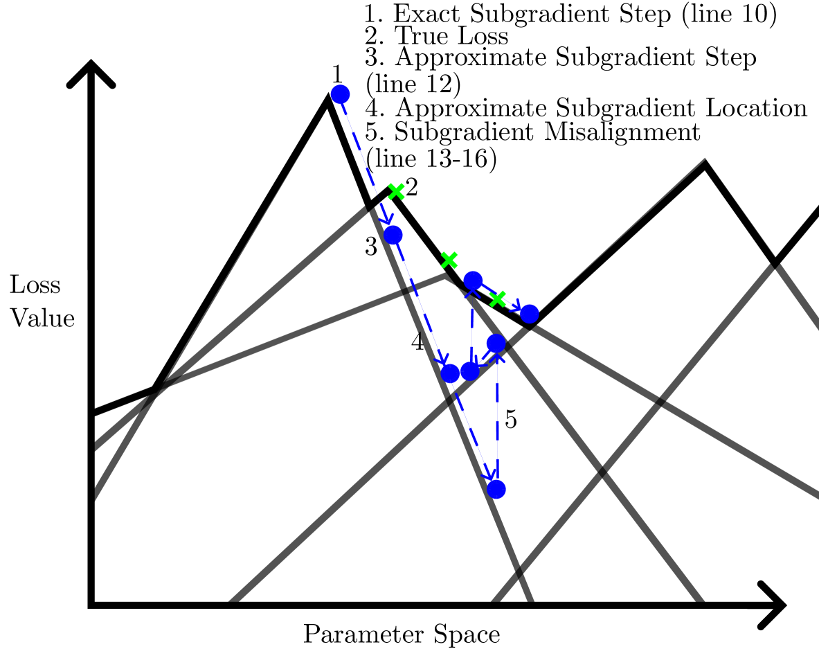
Figure 1: Graphical Representation of Algorithm 1.

4.1 Certificate and Compression Set Computation

We seek to minimize a loss function that encodes the barrier certificate conditions, with respect to the neural network parameters. To this end, for a $\tilde{\xi}\in\tilde{\Xi}$ and parameter vector $\theta$, let

$$L(\theta,\tilde{\xi})=l^{\Delta}(\theta,\tilde{\xi})+l^{s}(\theta),$$ (16)

represent an associated loss function comprised of sample-dependent loss $l^{\Delta}$, and sample-independent loss $l^{s}$

$$l^{s}(V_{\theta}) \vcentcolon=\frac{1}{|\mathcal{X}_{I}|}\sum_{x\in\mathcal{X}_{I}}\max\{0,V_{\theta}(x)\}$$

$$+\frac{1}{|\mathcal{X}_{U}|}\sum_{x\in\mathcal{X}_{U}}\max\{0,-V_{\theta}(x)\}.$$

$$l^{\Delta}(\theta,\tilde{\xi}) \vcentcolon=-\frac{1}{T}\Big{(}\inf_{x\in\mathcal{X}_{U}}B(x)-\sup_{x\in\mathcal{X}_{I}}B(x)\Big{)}$$

$$+\max_{k=1,\dots,M}\frac{B(x(t_{k}))-B(x(t_{k-1}))}{t_{k}-t_{k-1}}.$$

To instantiate these functions we consider a discrete set of grid-points on each sub-domain: $\mathcal{X}_{\overline{I}}$ is the set of points in the domain but outside the goal region, and $\mathcal{X}_{U}$ is the set of points in the unsafe set. These points are generated densely enough across the domain of interest, and hence offer an accurate approximation. Since these samples do not require access to the dynamics, we consider them separate to the sample-set $\{\tilde{\xi}^{i}\}_{i=1}^{N}$.

Consider the first summation in the sample-independent loss, if $B(x)<0$ then $\max\{0,B_{\theta}(x)\}=0$, i.e., no loss is incurred, implying satisfaction of (3). Under a similar reasoning, the other integral accounts for (4), respectively.

We impose the next mild assumption, a sufficient condition for termination of our algorithm.

Assumption 5 (Minimizers’ Existence).

For any $\{\tilde{\xi}\}_{i=1}^{N}$, and any non-empty $\mathcal{D}\subseteq\{\tilde{\xi}\}_{i=1}^{N}$, the set of minimizers of $\max_{\tilde{\xi}\in\mathcal{D}}L(\theta,\tilde{\xi}),$ is non-empty.

Note that, for a sufficiently expressive neural network, we can find a certificate $B$ which satisfies the state constraints and hence has a sample-independent loss of zero.

Algorithm 1 provides an inexact subgradient methodology to minimize the loss function, and to iteratively construct a compression set $\mathcal{C}$ (initially empty; see step $3$). We explain the main steps of this algorithm with reference to Figure 1. After an arbitrary parameter initialization, we follow the subgradient associated with the current sample in $\mathcal{C}$ (“blue” dot labeled by $3$). At this point, this step becomes inexact, as there would exist another sample resulting in a higher loss (“green” point labeled by $2$). Such a sample is in $\mathcal{M}$, step $9$ of Algorithm 1. However, the algorithm does not “jump” to the green point, as the condition in step $13$ of the algorithm is not yet satisfied. As such the algorithm performs inexact subgradient descent steps up to point $5$; this is the first instance where the condition in step $13$ is satisfied (there exists another constraint with opposite slope) and hence the algorithm “jumps” to a point with higher loss and subgradient of opposite sign. The “jumps” serve as an exploration step to investigate the non-convex landscape, while their number corresponds to the cardinality of the returned compression set. Such a procedure can be thought of as a constructive procedure for the general framework presented recently in [16] to construct compression sets.

In some cases, the parameter returned by Algorithm 1 may result in a value of the loss function greater than $-d$, and hence mean we are unable to verify safety. To achieve a lower loss, we make use of a sample-and-discarding procedure [6, 20], and introduce Algorithm 2 as an outer loop around Algorithm 1. This procedure leads to a lower loss, however the samples that are discarded have to be added to the compression set. Theorems 3 and 4 then apply, but with the compression set returned by Algorithm 2 instead.

To terminate our algorithm we require knowledge of $d$, but cannot calculate $d$ until we find $\theta^{\star}$. To resolve this, we propose two different approaches.

1. At every iteration $j$ calculate $d_{j}$ using the current best parameters $\theta_{j}$, terminate when $\max_{i}\left[L(\theta_{j},\tilde{\xi}^{i})\right]<d_{j}$.

2. Choose a parameter set $\Theta$, and take the supremum across the set to find an upper bound on $\mathcal{L}_{B},\mathcal{M}_{B}$, use these to calculate $d$.

To determine Lipschitz constants for neural networks we refer the reader to [4, 9, 22].

Algorithm 2 Compression Set Update with Discarding

1:Fix $\{\tilde{\xi}^{i}\}_{i=1}^{N}$

2:Set $\widetilde{\mathcal{C}}\leftarrow\varnothing$$\triangleright$ Initialise compression set

3:Set $\mathcal{D}\leftarrow\{\tilde{\xi}^{i}\}_{i=1}^{N}$ $\triangleright$ Initialise “running” samples

4:while $(\max_{\tilde{\xi}\in\mathcal{D}}l^{\Delta}(\theta,\tilde{\xi})>-d)\bigvee(l^{s}(\theta)>0)$ do

5:  $\theta,\mathcal{C}\leftarrow$ $\mathcal{A}(\theta,\mathcal{D})$ $\triangleright$ Call Algorithm 1

6:  $\widetilde{\mathcal{C}}\leftarrow\widetilde{\mathcal{C}}\cup\mathcal{C}$ $\triangleright$ Update $\widetilde{\mathcal{C}}$

7:  $\mathcal{D}\leftarrow\mathcal{D}\setminus\widetilde{\mathcal{C}}$ $\triangleright$ Discard $\widetilde{\mathcal{C}}$ from $\mathcal{D}$

8:return $\theta$, $\widetilde{\mathcal{C}}$

5 Numerical Results

We consider constructing a safety certificate for the nonlinear, two-dimensional jet engine model as considered in [15],

$$\dot{x}_{1}(t)=-x_{2}(t)-\frac{3}{2}x_{1}^{2}(t)-\frac{1}{2}x_{1}^{3}(t),\;\;\dot{x}_{2}(t)=x_{1}(t).$$ (17)

In Figure 3 we provide a graphical representation of the dynamics, sub-domains under study, the $0$-level set produced by our certificate, and the level sets calculated by the methods in [15] (one lower bounding the unsafe set, the other upper bounding the initial set). We used $5$ independent repetitions (each with different multi-samples) of $1,000$ sampled trajectories and $367$ seconds of computation time (standard deviation $139$s), to obtain $\varepsilon=0.01492$ (standard deviation $0.00140$) with confidence to $0.99$. The methodology of [15] required $257149$ state pair samples and $5123$ seconds (standard deviation $449$s) of computation time to compute a barrier certificate with the same confidence (however, this holds deterministically). We estimate the Lipschitz constants using the methods in [23]. Figure 3 contains a 3D plot of the certificate.

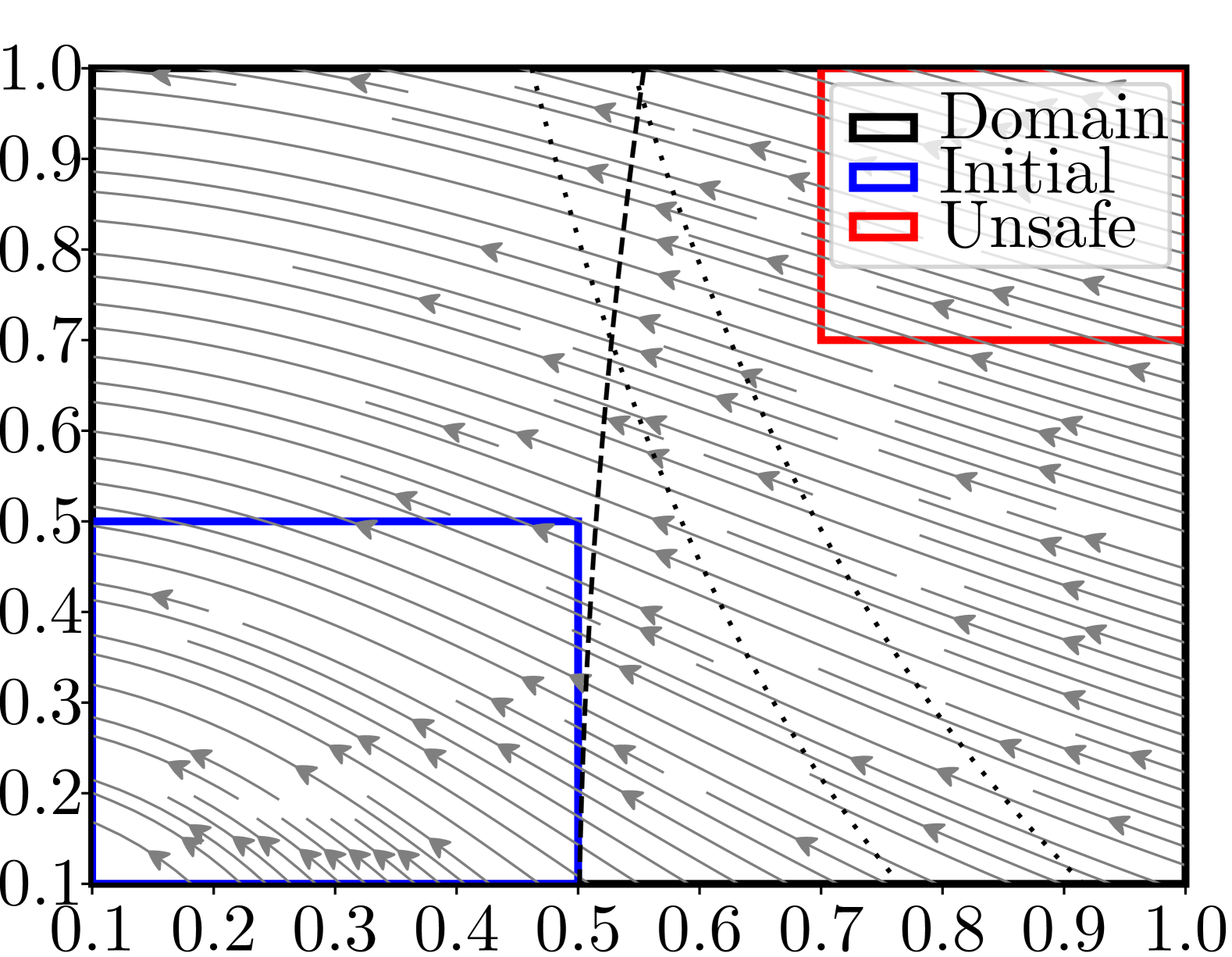
Figure 2: Phase plane plot, initial and unsafe set for (17). The zero-level set for our certificate is dashed; level sets that bound the initial and unsafe sets (i.e. $\gamma$- and $\lambda$- level sets) in [15] are dotted.

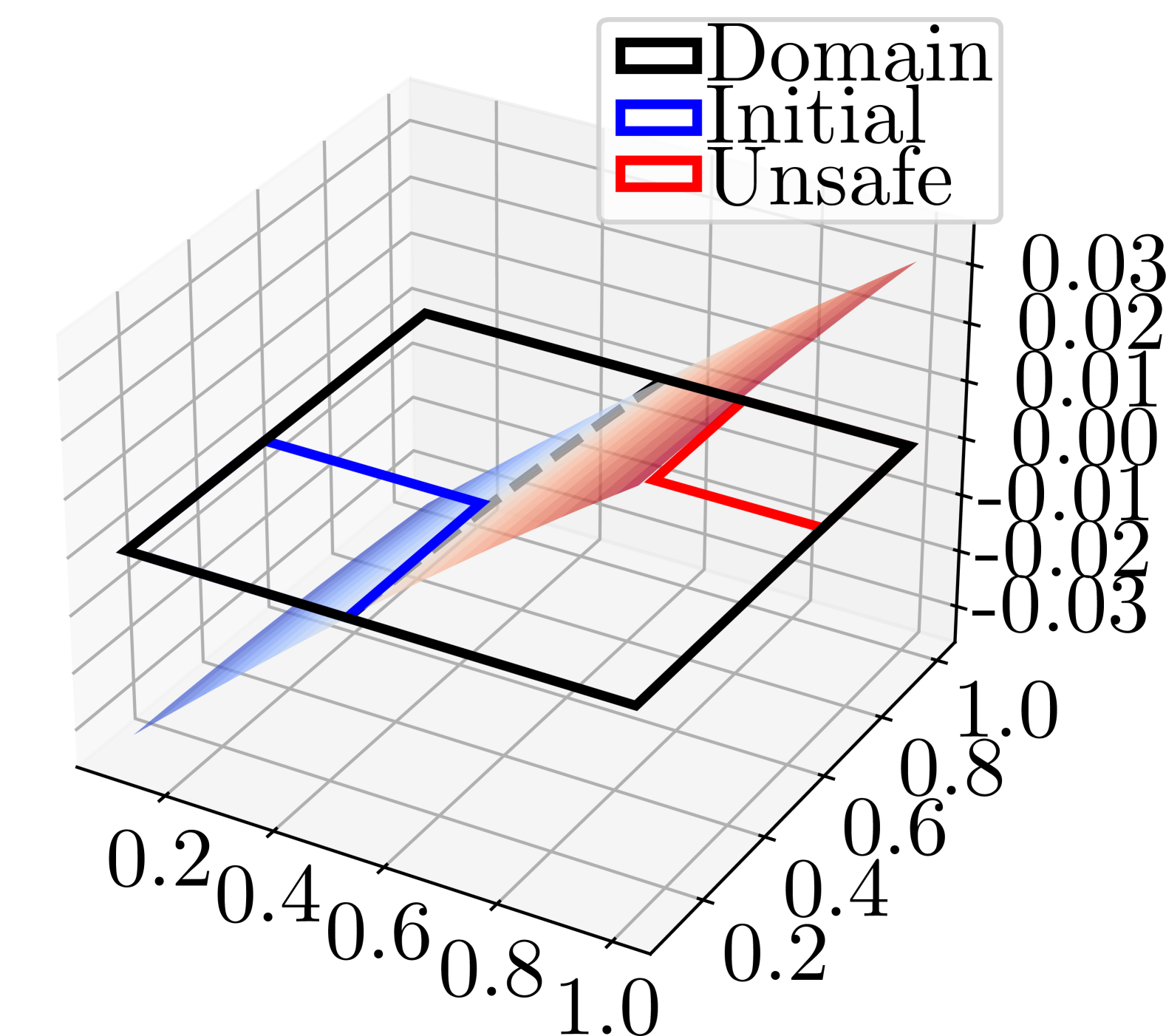
Figure 3: Surface plot of the safety/barrier certificate, generated by our techniques, for the system of Figure 3.

Beyond these numerical results, we briefly discuss the theoretical differences between our approaches. The results in [15] offer a guarantee that, with a certain confidence, the safety property is always satisfied, in contrast to Theorem 4 where we provide such guarantees in probability (up to a quantifiable risk level $\varepsilon$). However, these “always” guarantees, albeit very useful, come with some challenges. Firstly, they are not applicable when part of the initial set is unsafe. Secondly, they implicitly require some knowledge of the underlying probability distribution. Finally, they are bound to an exponential growth with the dimension of the state space.

Related to this last point, we performed a comparison on the following four-dimensional system taken from [8].

$$\dot{x}_{1}(t) =x_{1}(t)+\frac{x_{1}(t)x_{2}(t)}{5}-\frac{x_{3}(t)x_{4}(t)}{2},$$ (18)

$$\dot{x}_{2}(t) =\cos(x_{4}(t)),$$

$$\dot{x}_{3}(t) =0.01\sqrt{|x_{1}(t)|},$$

$$\dot{x}_{4}(t) =-x_{1}(t)-x_{2}(t)^{2}+\sin(x_{4}(t)).$$

We calculate that the approach of [15] requires at least $10^{19}$ samples to return a confidence lower bounded by at most $10^{-30}$, which is not practically useful. In contrast, our techniques with only $100$ samples obtain a risk level of $\varepsilon=0.21450$ (standard deviation $0.00910$), confidence $1-10^{-5}$.

6 Conclusion

We have proposed a method for synthesis of neural-network certificates for continuous-time dynamical systems, based only on a finite number of trajectories from a system. Our numerical experiments demonstrate the efficacy of our methods on a number of examples, involving comparison with related methodologies in the literature. Current work concentrates towards extending our analysis to controlled systems, thus co-designing a controller and a certificate at the same time.

APPENDIX

1 Proof of Theorem 4

We aim at finding a bound on the discretisation gap $L(\theta,\xi)-L(\theta,\tilde{\xi})$ so that, for sufficiently small loss evaluated on the time-discretised approximations $L(\theta,\tilde{\xi})$, we also achieve a negative loss on the continuous trajectories $L(\theta,\xi)$.

$$L(\theta,\xi)-L(\theta,\tilde{\xi})=l^{\Delta}(\theta,\xi)-l^{\Delta}(\theta,\tilde{\xi})$$

$$=\max_{x\in\xi}\evaluated{\frac{dB}{dt}}_{x}-\max_{k=1,\dots,M}\frac{B(x(t_{k}))-B(x(t_{k-1}))}{t_{k}-t_{k-1}}.$$ (19)

Replacing the first maximisation with one between time instances, and exchanging the order of the $\max$ operators, (19) is equal to

$$\max_{k=1,\dots,M}\max_{t\in[t_{k-1},t_{k}]}\evaluated{\frac{dB}{dt}}_{x(t)}$$ (20)

$$\qquad-\max_{k=1,\dots,M}\frac{B(x(t_{k}))-B(x(t_{k-1}))}{t_{k}-t_{k-1}},$$

$$\leq\max_{k=1,\dots,M}\Bigg{[}\max_{t\in[t_{k-1},t_{k}]}\evaluated{\frac{dB}{dt}}_{x(t)}-\frac{B(x(t_{k}))-B(x(t_{k-1}))}{t_{k}-t_{k-1}}\Bigg{]}.$$ (21)

We can now replace the difference term with an integral, so that (21) becomes equivalent to

$$\max_{k=1,\dots,M}\frac{\int_{t_{k-1}}^{t_{k}}\max_{t\in[t_{k-1},t_{k}]}\evaluated{\frac{dB}{dt}}_{x(t)}-\evaluated{\frac{dB}{dt}}_{x(\tau)}~\mathrm{d}\tau}{t_{k}-t_{k-1}}.$$

Letting $\mathfrak{L}=\mathcal{M}_{B}\mathcal{L}_{f}+\mathcal{M}_{f}\mathcal{L}_{B}$ (refer to (14) for the definition of the various constants), the previous derivations lead to

$$L(\theta,\xi)-L(\theta,\tilde{\xi})$$

$$\leq\max_{k=1,\dots,M}\frac{\int^{t_{k}}_{t_{k-1}}\|x(\tau)-\max_{t\in[t_{k-1},t_{k}]}x\|\mathfrak{L}~\mathrm{d}\tau}{t_{k}-t_{k-1}}$$

$$\leq\max_{k=1,\dots,M}\mathfrak{L}\frac{\int_{t_{k}}^{t_{k-1}}\mathcal{M}_{f}(t_{k}-t_{k-1})~\mathrm{d}\tau}{t_{k}-t_{k-1}},$$ (22)

$$=\max_{k=1,\dots,M}\mathfrak{L}\int_{t_{k}}^{t_{k-1}}\mathcal{M}_{f}~\mathrm{d}\tau=\overline{t}\mathfrak{L}\mathcal{M}_{f}.$$ (23)

where the second inequality is since $\sup_{x}\|f(x)\|\leq\mathcal{M}_{f}$, and the last one since $\overline{t}=\max_{k=1,\dots,M}(t_{k}-t_{k-1})$.

This results then to a discretisation gap as in (14). By Theorem 3, and noticing that violating the conditions with $\psi^{\Delta}_{d}$ in place of $\psi^{\Delta}$, is equivalent to $L(\theta^{\star},\tilde{\xi})>-d$, we have

$$\mathbb{P}^{N}\left\{\{\tilde{\xi}^{i}\}_{i=1}^{N}\colon\mathbb{P}\{\tilde{\xi}\colon L(\theta^{\star},\tilde{\xi})>-d\}\leq\varepsilon(C_{N},\beta,N)\right\}\geq 1-\beta.$$

Since $L(\theta^{\star},\xi)\leq L(\theta^{\star},\tilde{\xi})+d$, this then implies that

$$\mathbb{P}^{N}\left\{\{\tilde{\xi}^{i}\}_{i=1}^{N}\colon\mathbb{P}\{\xi\colon L(\theta^{\star},\xi)>0\}\leq\varepsilon(C_{N},\beta,N)\right\}\geq 1-\beta,$$

thus concluding the proof. ∎

References

- [1] Alessandro Abate. Formal verification of complex systems: model-based and data-driven methods. In MEMOCODE, pages 91–93. ACM, 2017.
- [2] Aaron D. Ames, Samuel Coogan, Magnus Egerstedt, Gennaro Notomista, Koushil Sreenath, and Paulo Tabuada. Control barrier functions: Theory and applications. In ECC, pages 3420–3431. IEEE, 2019.
- [3] Thom S. Badings, Licio Romao, Alessandro Abate, David Parker, Hasan A. Poonawala, Mariëlle Stoelinga, and Nils Jansen. Robust control for dynamical systems with non-gaussian noise via formal abstractions. Journal of Artificial Intelligence Research, 76:341–391, 2023.
- [4] Aritra Bhowmick, Meenakshi D’Souza, and G. Srinivasa Raghavan. LipBaB: Computing exact lipschitz constant of ReLU networks. In ICANN (4), volume 12894 of Lecture Notes in Computer Science, pages 151–162. Springer, 2021.
- [5] Marco Campi and Simone Garatti. Introduction to the Scenario Approach. SIAM Series on Optimization, 2018.
- [6] Marco C. Campi and Simone Garatti. A sampling-and-discarding approach to chance-constrained optimization: Feasibility and optimality. Journal of Optimization Theory and Applications, 148(2):257–280, 2011.
- [7] Marco C. Campi and Simone Garatti. Compression, generalization and learning. J. Mach. Learn. Res., 24:339:1–339:74, 2023.
- [8] Alec Edwards, Andrea Peruffo, and Alessandro Abate. Fossil 2.0: Formal certificate synthesis for the verification and control of dynamical models. In HSCC, pages 26:1–26:10. ACM, 2024.
- [9] Mahyar Fazlyab, Alexander Robey, Hamed Hassani, Manfred Morari, and George J. Pappas. Efficient and accurate estimation of lipschitz constants for deep neural networks. In NeurIPS, pages 11423–11434, 2019.
- [10] Simone Garatti and Marco C. Campi. Risk and complexity in scenario optimization. Math. Program., 191(1):243–279, 2022.
- [11] Takafumi Kanamori and Akiko Takeda. Worst-case violation of sampled convex programs for optimization with uncertainty. J. Optim. Theory Appl., 152(1):171–197, 2012.
- [12] Alexandar Kozarev, John F. Quindlen, Jonathan P. How, and Ufuk Topcu. Case studies in data-driven verification of dynamical systems. In HSCC, pages 81–86. ACM, 2016.
- [13] Kostas Margellos, Maria Prandini, and John Lygeros. On the connection between compression learning and scenario based single-stage and cascading optimization problems. IEEE Trans. Autom. Control., 60(10):2716–2721, 2015.
- [14] Peyman Mohajerin Esfahani, Tobias Sutter, and John Lygeros. Performance bounds for the scenario approach and an extension to a class of non-convex programs. IEEE Transactions on Automatic Control, 60(1):46–58, 2015.
- [15] Ameneh Nejati, Abolfazl Lavaei, Pushpak Jagtap, Sadegh Soudjani, and Majid Zamani. Formal verification of unknown discrete- and continuous-time systems: A data-driven approach. IEEE Trans. Autom. Control., 68(5):3011–3024, 2023.
- [16] Dario Paccagnan, Marco C. Campi, and Simone Garatti. The pick-to-learn algorithm: Empowering compression for tight generalization bounds and improved post-training performance. In NeurIPS, 2023.
- [17] Antonis Papachristodoulou and Stephen Prajna. On the construction of Lyapunov functions using the sum of squares decomposition. In CDC, pages 3482–3487. IEEE, 2002.
- [18] Stephen Prajna and Ali Jadbabaie. Safety verification of hybrid systems using barrier certificates. In HSCC, volume 2993 of Lecture Notes in Computer Science, pages 477–492. Springer, 2004.
- [19] Luke Rickard, Alessandro Abate, and Kostas Margellos. Data-driven neural certificate synthesis. CoRR, abs/2502.05510, 2025.
- [20] Licio Romao, Antonis Papachristodoulou, and Kostas Margellos. On the exact feasibility of convex scenario programs with discarded constraints. IEEE Trans. Autom. Control., 68(4):1986–2001, 2023.
- [21] Ali Salamati, Abolfazl Lavaei, Sadegh Soudjani, and Majid Zamani. Data-driven verification and synthesis of stochastic systems via barrier certificates. Autom., 159:111323, 2024.
- [22] Aladin Virmaux and Kevin Scaman. Lipschitz regularity of deep neural networks: Analysis and efficient estimation. In NeurIPS, pages 3839–3848, 2018.
- [23] Graham R. Wood and B. P. Zhang. Estimation of the Lipschitz constant of a function. 8(1):91–103, 1996.