Engineering tunable fractional Shapiro steps in colloidal transport

Shapiro steps are quantized plateaus in the velocity-force or velocity-torque curve of a driven system, when its speed remains constant despite an increase in the driving force. For microscopic particles driven across a sinusoidal potential, integer Shapiro steps have been observed. By driving a single colloidal particle across a time-modulated, non-sinusoidal periodic optical landscape, we here demonstrate that fractional Shapiro steps emerge in addition to integer ones. Measuring the particle position via individual particle tracking, we reveal the underlying microscopic mechanisms that produce integer and fractional steps and demonstrate how these steps can be controlled by tuning the shape and driving protocol of the optical potential. The flexibility offered by optical engineering allows us to generate wide ranges of potential shapes and to study, at the single-particle level, synchronization behavior in driven soft condensed matter systems.

Many physical systems driven out-of-equilibrium by an external force are characterized in terms of a velocity-frequency or velocity-force relation [1, 2, 3, 4], which is an analogue of the current-voltage characteristic measured in superconducting junctions [5, 6], carbon nanotubes [7, 8, 9], graphene [10, 11] and other electronic circuits [12]. When subjected to a time-periodic force, the internal dynamics of these systems may synchronize with the external driving. The synchronization effect manifests itself in the form of constant plateaus of voltage or velocity versus mean current or force. Such plateaus, known as Shapiro steps, were first reported for a superconducting Josephson junction driven by a microwave signal [13, 14], where discrete steps in the voltage arise from the synchronization between the applied signal and oscillations of the Josephson phase [15, 16].

Since their discovery, understanding the nature of Shapiro steps has been important not only for elucidating basic mechanisms underlying superconductivity, but also for new technological developments including, for example, the realization of metrological voltage controllers [17, 18].

In classical driven systems, the presence of discrete steps in the velocity-force curves can be the signature of different physical effects, from speed reduction due to friction [19, 20, 21], to the onset of a pinning-depinning transition [22, 23], synchronization [24, 25] or locking [26, 27, 28] with an underlying energetic landscape. In many-particle systems, collective particle motions through periodic [29, 30, 31, 32] or random [33, 34] landscapes are often mediated by defects, which move like a single particle and display a complex sequence of plateaus with integer or fractional values of their speed. Due the subtle interplay of interparticle and particle-substrate interaction, defect propagation takes place in complex periodic energy landscapes.

Modern advancements in optical manipulation of microscale matter have made it possible to engineer such potentials with tunable energetic wells and inter-well distances [35, 36, 37]. With this capability one can manipulate and drag microscopic particles [38, 39], biological systems [40, 41], measure tiny forces [42, 43], or even assemble matter in two [44, 45] or three dimensions [46, 47, 48]. In this context, integer Shapiro steps have been recently reported for a single colloidal particle driven through an optical sinusoidal potential by an underlying oscillating substrate [49]. The plateaus emerged due to dynamic mode locking [24], where synchronization with the oscillating substrate leads to a sequence of transport modes characterized by a constant speed.

By engineering non-sinusoidal periodic potentials with several maxima per wavelength, we show here that a single particle can display integer and fractional steps in the average speed under time-dependent driving. Employing individual particle tracking, we unveil the microscopic mechanisms leading to the emergence of these steps, and show how it is possible to control them by constructing diagrams of phase-locked modes. Our driving strategy implements the time modulation directly within the periodic potential, without the need to translate or oscillate the substrate which could induce delay in the particle response and hydrodynamic back-flow. The non-sinusoidal shape allows the particle to synchronize with the driving potential in a variety of modes, generating both pronounced integer and fractional Shapiro steps. Using our ability to tune the optical landscape and the driving protocol, we can even increase the prominence of some fractional Shapiro steps over others.

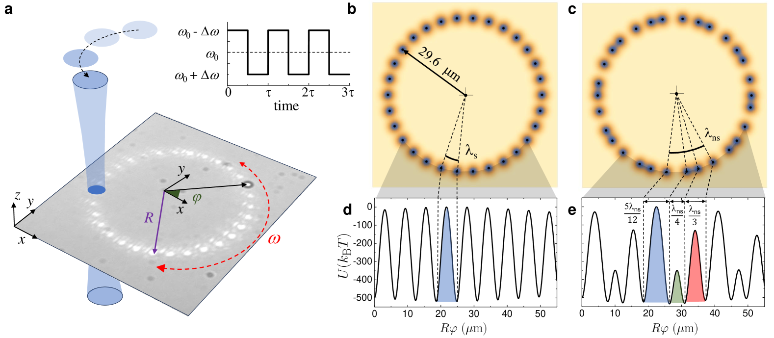
Figure 1: Time-modulated sinusoidal and non-sinusoidal optical potentials. a, Colloidal particle driven along a rotating ring of optical traps created by fast scanning tweezers. The ring rotates with a time-dependent angular frequency $\omega(t)$ modulated according to a square wave. Inset at the top displays the modulation with period $\tau$ and amplitude $\Delta\omega$ around a mean frequency $\omega_{0}$. b,c, Density plots of $N_{\rm tr}=30$ optical traps with positions on a circle of radius $R=29.6\,\rm{\mu m}$. In b, the optical traps are arranged equidistantly and create a sinusoidal potential with wavelength $\lambda_{\rm s}=2\pi R/30$ along the ring. In c, the traps are arranged in 10 groups of triplets, yielding a periodic non-sinusoidal potential with wavelength $\lambda_{\rm ns}=2\pi R/10$. In each triplet, spacing between neighboring traps are $5\lambda_{\rm ns}/12$, $\lambda_{\rm ns}/4$ and $\lambda_{\rm ns}/3$. d,e, Corresponding profiles of the optical potential $U$ extracted from torque measurements. Supplementary Videos 1-6 in the Supporting Information show representative motions of the particle in these two potentials.

Designing time-modulated periodic
optical potentials

We drive a single polystyrene colloidal particle of diameter $\sigma=4\,\rm{\mu m}$ across a time-dependent periodic potential generated by passing an infrared continuous-wave laser through a pair of acousto-optic deflectors, as sketched in Fig. 1a. The particles sediment close to the bottom surface where they float due to balance between gravity and electrostatic repulsive interactions. Since the particles are illuminated by the laser from the top, they are trapped in two dimensions, i.e. close to the bottom plane. Technical details are given in the Methods Section.

The laser is rapidly steered through $N_{\rm tr}=30$ positions on a circle of radius $R=29.6\,\rm{\mu m}$. Each trap position is visited every $20\,\rm{\mu s}$ [50, 51, 52], a time scale much smaller than the self-diffusion time of the particle in the absence of driving, $\sigma^{2}/D\sim 267\,{\rm s}$, where $D\sim 0.057\,\rm{\mu m^{2}\,s^{-1}}$ is the self-diffusion coefficient. As the scanning is much faster than the particle motion, the particle feels an effective, quasistatic potential. When a laser passes through a position along the circle, its spot creates a Gaussian potential well with a depth proportional to the laser power. As described in the Methods section, the periodic potential felt by the colloidal particle results from the superposition of these Gaussian wells.

We engineer two types of periodic potentials, a sinusoidal one $U_{\rm s}$ with wavelength $\lambda_{\rm s}=2\pi R/30$, Fig. 1b,d, and a non-sinusoidal one $U_{\rm ns}$ with wavelength $\lambda_{\rm ns}=3\lambda_{\rm s}$, Fig. 1c,e. The $U_{\rm ns}$ is generated by placing the traps in groups of three per wavelength $\lambda_{\rm ns}$, with trap centers located at positions $0$, $\lambda_{\rm ns}/3$, and $7\lambda_{\rm ns}/12$ in $[0,\lambda_{\rm ns})$. With this arrangement, we obtain three distinct potential wells per wavelength $\lambda_{\rm ns}$ with inter-well spacings $\lambda_{\rm ns}/3$, $\lambda_{\rm ns}/4$, and $5\lambda_{\rm ns}/12$. The profiles of the periodic potentials are calculated from measured particle trajectories, see Methods Section for details. These profiles, shown in Fig. 1d for the sinusoidal potential and in Fig. 1e for the non-sinusoidal one, exhibit energetic barriers of about $500\,k_{\rm B}T$. Thus, thermal fluctuations are rather weak in our system.

The selected distances between the optical traps were chosen such that the overlap of the Gaussian potential wells generate a simple periodic but non-sinusoidal potential able to induce integer and fractional Shapiro steps in the particle current. The distance between the potential wells where chosen such that it allows to generate two potential wells each of them able to stably trap a colloidal particle. Indeed, distance smaller than the particle diameter could have been not distinguished as different by the particle which would feel them as a single, larger well rather than two distinct ones. On the other hand, potential wells very far from each other could be unable to stably trap the particle along a ring, due to small but still present thermal fluctuations along the radial direction.

By rotating all traps with an angular speed $\omega$, the particle is driven along the circle, as illustrated in Fig. 1a. For inducing Shapiro steps in the average particle velocity, $\omega$ is modulated periodically in time with period $\tau$, yielding a time-modulated driving of the particle. Specifically, as shown in Fig. 1a, we apply a square-wave protocol with mean frequency $\omega_{0}$ and amplitude $\Delta\omega$: $\omega(t)=\omega_{0}+\Delta\omega$ for $t\in[n\tau,(n+1/2)\tau)$ and $\omega(t)=\omega_{0}-\Delta\omega$ for $t\in[(n+1/2)\tau,(n+1)\tau)$, $n=0,1,2,\ldots$.

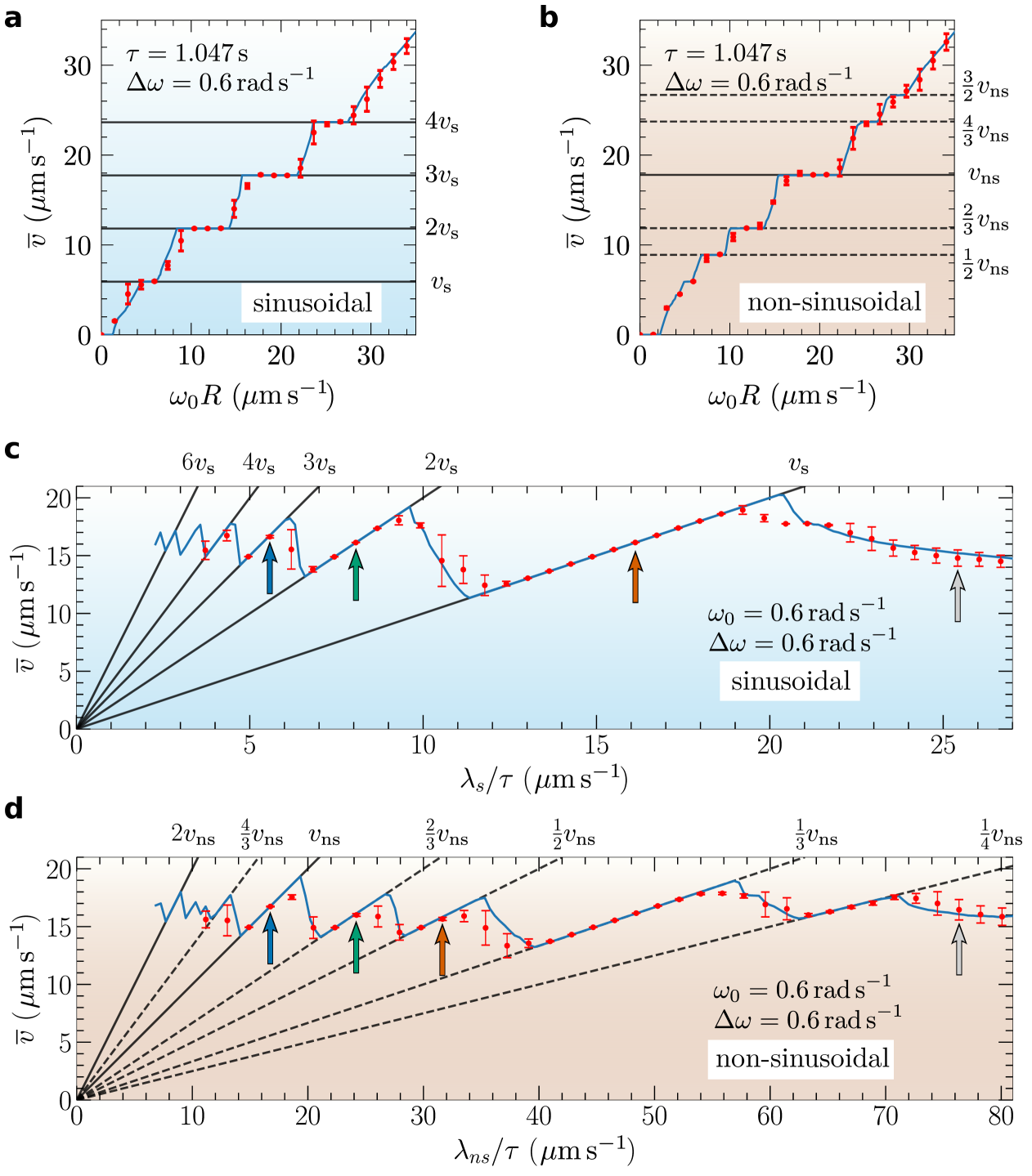
Figure 2: Phase-locked mean particle velocities reflecting motion synchronized with the driving. a,b, Average velocity $\bar{v}$ in the corotating frame versus mean azimuthal velocity $\omega_{0}R$ of trap rotation for the sinusoidal (a) and the periodic but non-sinusoidal optical potential (b). In both images we vary $\omega_{0}$ at fixed $R=29.6\rm{\mu m}$, $\tau=1.047\,{\rm s}$, and $\Delta\omega=0.6\,{\rm rad\,s}^{-1}$. c,d, Average velocity $\bar{v}$ as a function of the characteristic oscillatory driving velocities $\lambda_{\rm s}/\tau=v_{\rm s}$ and $\lambda_{\rm ns}/\tau=v_{\rm ns}$ for the sinusoidal potential (c) and the non-sinusoidal one (d). In both images we vary $\tau$ at fixed $\omega_{0}=\Delta\omega_{0}=0.6\,{\rm{rad}\,s}^{-1}$, and $R=29.6\,\rm{\mu m}$. In all graphs scattered red dots are experimental data, the error bars denote the standard deviation of three experimental measurements, and blue lines are results from numerical simulations. Continuous black lines mark integer steps and dashed lines mark fractional ones. Values on top of the graphs in c,d indicate slopes $n$ and $p/q$ of the lines according to equations (1) and (2), the colored arrows denote measurements, whose particle trajectories are shown in Fig. 3.

Shapiro steps in mean particle velocity

For a constant angular velocity $\omega_{0}$, the particle trapped in one of the potential wells tends to follow the trap rotation in clockwise direction but experiences a resistance due to the Stokesian friction exerted by the surrounding water. This friction gives rise to a torque in counter-clockwise direction. Since this torque is a constant proportional to $\omega_{0}$ in a frame corotating with the traps, we analyze the particle motion in this frame. The average velocity $\bar{v}$ along the tangential direction in the corotating frame corresponds to an average velocity $\bar{v}_{\rm lab}=\bar{v}-\omega_{0}R$ in the laboratory frame.

Applying the square-wave modulation $\omega(t)$, we measure $\bar{v}$ for both the sinusoidal [Fig. 1d] and the non-sinusoidal potential [Fig. 1e]. Figures 2a,b show results of these measurements for varying $\omega_{0}$ at fixed period $\tau=1.047\,$\mathrm{s}$$ and amplitude $\Delta\omega=0.6\,$\mathrm{r}\mathrm{a}\mathrm{d}\,\mathrm{s}^{-1}$$ of the driving (red circles with error bars). In both figures, intervals of $\omega_{0}$ occur, where $\bar{v}$ remains constant corresponding to a sequence of Shapiro steps. In these plateau regimes of constant $\bar{v}$, the particle synchronizes its motion with the oscillatory driving, leading to phase-locked particle velocities in the corotating reference frame. The experimental results are in excellent agreement with Brownian dynamics simulations (blue lines) detailed in the Methods Section.

For the sinusoidal potential [Fig. 2a], all steps are integer multiples of the characteristic speed $v_{\rm s}=\lambda_{\rm s}/\tau=5.92\,$\mu\mathrm{m}\,\mathrm{s}^{-1}$$ of the driving, yielding phase-locked values

$$v_{n}=nv_{\rm s},\quad n=1,2,\ldots$$ (1)

These steps are indicated by the horizontal black lines in Fig. 2a for $n=1,\ldots 4$. While not all steps are equally well pronounced, only integer plateaus were observed. These steps arise from a synchronized particle motion, where in one period $\tau$ of the driving, the particle is displaced by $n$ wavelengths $\lambda_{\rm s}$ of the sinusoidal potential.

For the non-sinusoidal potential [Fig. 2b], we observe steps (dashed horizontal black line)

$$v_{p,q}=\frac{p}{q}\,v_{\rm ns}\,\,\,.$$ (2)

which are a fractions $p/q$ of the characteristic velocity $\bar{v}=v_{\rm ns}=\lambda_{\rm ns}/\tau=17.76\,$\mu\mathrm{m}\,\mathrm{s}^{-1}$$. Also, the integer step with $\bar{v}=v_{\rm ns}=\lambda_{\rm ns}/\tau$ occurs (solid horizontal black line). The fractional plateaus arise from a synchronized particle motion, where in $q$ periods $\tau$ of the driving, the particle is displaced by $p$ wavelengths $\lambda_{\rm ns}$ of the non-sinusoidal potential.

The fractional plateaus are smaller than integer ones, and thus more challenging to be resolved. In our experiments, we increased $\omega_{0}R$ in steps of $1.5\,$\mu\mathrm{m}\,\mathrm{s}^{-1}$$. For this resolution, none of the fractional steps in Fig. 2b covers an interval of $\omega_{0}R$ consisting of more than two experimental points. However, the numerical simulations shown by the blue lines in Figs. 2b provide evidence of the presence of the fractional steps in the non-sinusoidal potential in Fig. 2b.

Nonetheless, to unambiguously demonstrate synchronized motion with phase-locked velocities according to equations (1) and (2) in our experiments, we can also keep $\omega_{0}$ and $\Delta\omega$ fixed and vary the period $\tau$ of the driving. For a good choice of $\omega_{0}$ and $\Delta\omega$, the driving should be such that the particle can surmount the potential barriers at the square wave’s high value $\omega_{0}+\Delta\omega$, while it remains trapped in a potential well at the low value $\omega_{0}-\Delta\omega$. This can be ensured for the trapping by taking $\Delta\omega=\omega_{0}$. For surmounting barriers, we choose $\omega_{0}=0.6\,{\rm rad\,s}^{-1}$, which is comparable to the critical frequency at which the particle starts slipping in the potential.

Figures 2c,d show the mean particle velocity as a function of the characteristic velocities $\lambda_{\rm s}/\tau$ and $\lambda_{\rm ns}/\tau$ for $\omega_{0}=\Delta\omega=0.6\,{\rm rad\,s}^{-1}$. Now, phase-locking according to Eqs. (1) and (2) manifests itself as $\bar{v}$ varying linearly with $v_{\rm s}=\lambda_{\rm s}/\tau$ and $v_{\rm ns}=\lambda_{\rm ns}/\tau$. Fractional phase locking in Fig. 2d is much more clearly visible than in Fig. 2b: a linear increase of $\bar{v}$ with $\lambda_{\rm ns}/\tau$ occurs in broad intervals with fractional slopes $p/q=1/4$, $1/3$, $1/2$, and $2/3$. Again, simulations (blue lines) in both Figs. 2c,d are in excellent agreement with the experimental observations.

The error bars in Figs. 2a-d represent the spread between three different sets of measurements, each conducted with a different particle from the same stock solution. They are relatively small when the particle is phase-locked with the oscillating potential and become larger when it is not. This can be understood from the fact that for synchronized motion, fluctuations of the particle position due to thermal noise are suppressed. The effect is reflected in a lower diffusion coefficient of the particle in a phase-locked state [53].

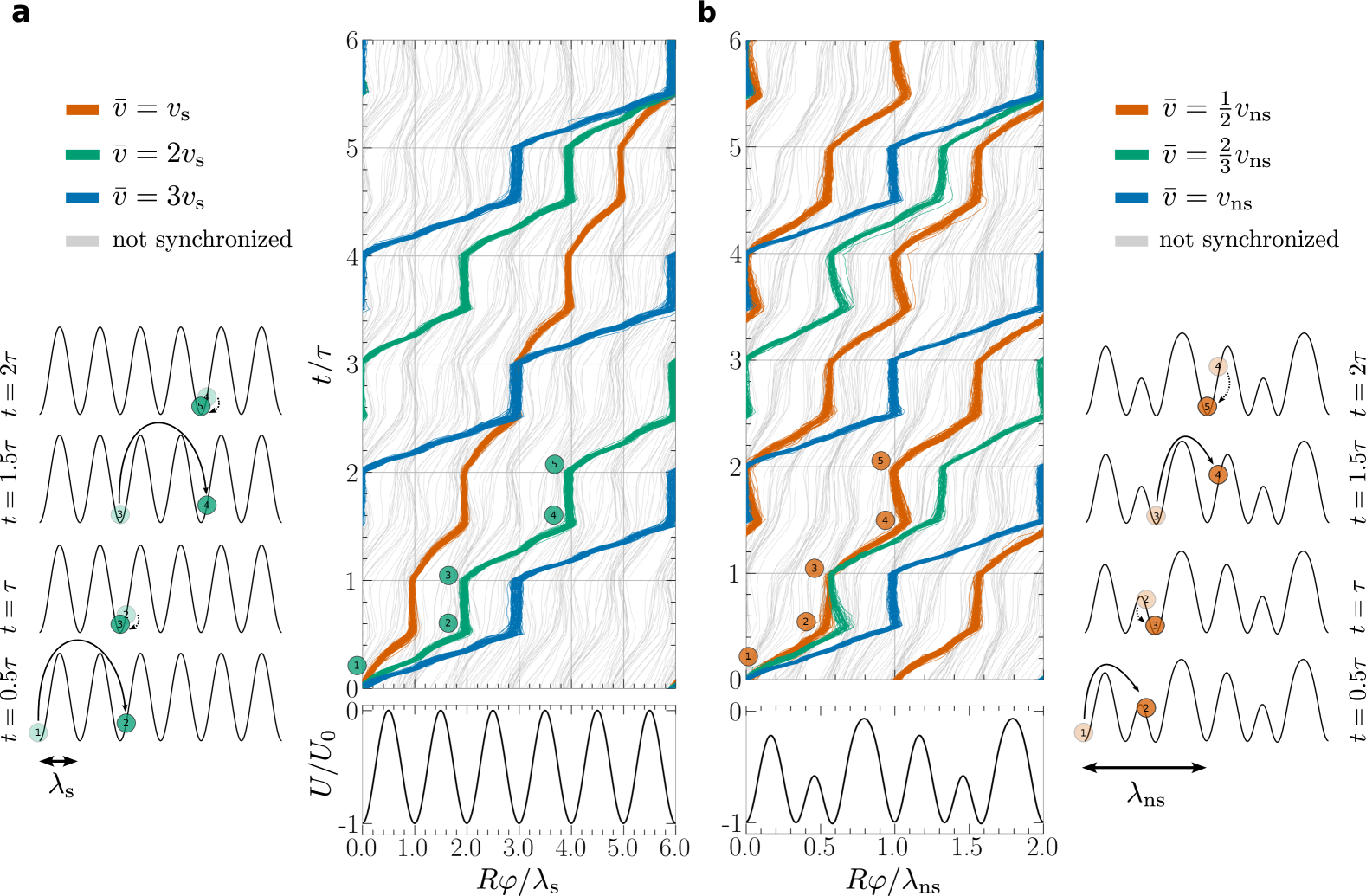
Figure 3: Synchronized and non-synchronized particle trajectories. a,b, Scaled angular particle positions $R\varphi/\lambda_{\rm s,ns}$ versus scaled time $t/\tau$ in the corotating reference frame at fixed $\omega_{0}=\Delta\omega=0.60\,$\mathrm{r}\mathrm{a}\mathrm{d}\,\mathrm{s}^{-1}$$ as in Figs. 2c,d for (a) the sinusoidal and (b) the non-sinusoidal potential for various driving frequencies $1/\tau$. The chosen frequencies correspond to values of $\lambda_{\rm s}/\tau$ and $\lambda_{\rm ns}/\tau$ indicated by the colored arrows in Figs. 2c,d. Optical potentials are shown at the bottom. Trajectories are displayed in a reduced zone scheme, i.e. when they exit at the right side of the graph they are continued at the left side. Synchronized trajectories corresponding to Shapiro steps overlap and are colored in orange, green and blue. Non-synchronized trajectories are marked in gray. In a, mean velocities $\bar{v}$ obtained from the synchronized trajectories are integer multiples of $v_{\rm s}$. In b, fractions $p/q$ of $v_{\rm ns}$ appear, which correspond to particle displacements by $p$ wavelengths $\lambda_{\rm ns}$ in $q$ periods of the driving. The small schematics on the side of the images illustrate the particle position within the periodic potential corresponding to an integer step (side of a) and to a fractional one (side of b). The videos 1-6 in the Supplementary Information show the synchronized particle motion across the periodic potentials.

The ability to precisely track the colloidal particle allows us to analyze in detail its movement across the two types of periodic potentials. In Fig. 3 we show particle trajectories for various driving frequencies $1/\tau$ at fixed $\omega_{0}=\Delta\omega$ for the sinusoidal (Fig. 3a) and non-sinusoidal potential (Fig. 3b).

Colored synchronized trajectories collapse onto space-time periodic limit cycles apart from thermal fluctuations. Along the synchronized trajectories in Fig. 3a, the particle moves $n=1,2,3$ wavelengths $\lambda_{\rm s}$ in one period $\tau$ of the driving, giving a mean particle velocity $\bar{v}=nv_{\rm s}$. Along the synchronized trajectories in Fig. 3b, the particle moves $p$ wavelengths $\lambda_{\rm ns}$ in $q$ periods $\tau$, giving the mean particle velocity $\bar{v}=(p/q)v_{\rm ns}$ with fractions $p/q=1/2$, $2/3$, $1/1$. Grey lines in both graphs correspond to particle trajectories that are not synchronized with the driving. In the schematics on the sides of Fig. 3, we illustrate the particle displacements in successive half periods $\tau/2$ for the phase-locked modes with $n=2$ in Fig. 3a and $p/q=2/3$ in Fig. 3b.

For the sinusoidal potential, we see that integer Shapiro steps with $\bar{v}=v_{\rm s},2v_{\rm s},\ldots$ occur when the particle is trapped in a potential minimum for half a period of the driving, and then moves a distance $\lambda_{\rm s},2\lambda_{\rm s},\ldots$ in the other half. The trapping at the minimum aids the synchronization as a way of “resetting” the particle position during each period.

An analogous situation occurs for the non-sinusoidal potential, but now the particle displays an additional backward or forward movement to reach the closest potential minimum. These additional movements can be seen, for example, in the bunches of orange particle trajectories in Fig. 3b, which correspond to the step at $\bar{v}=\frac{1}{2}v_{\rm ns}$ in Fig. 2b.

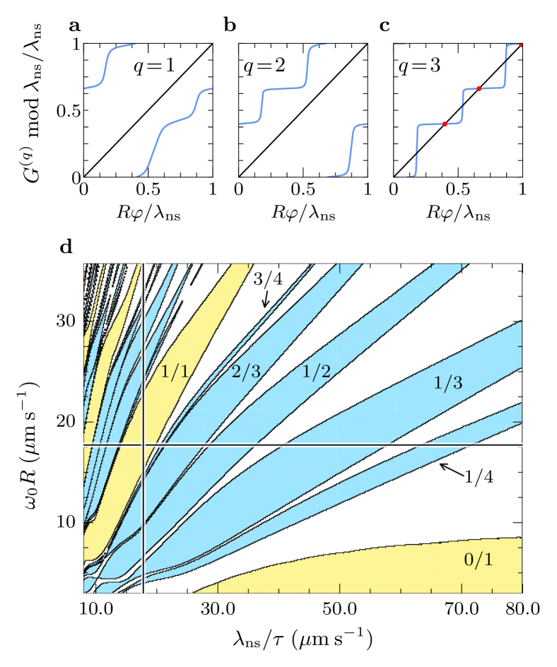
Figure 4: Diagram of phase-locked modes. a-c, Propagators $G^{(q)}(x)$ giving position of the particle after $q$ periods of the driving if it started at $x$. Parameters are as in Fig. 2d when $\lambda_{\rm ns}/\tau=50\,\mu{\rm m\,s}^{-1}$. Intersections of $G^{(3)}(x)$ with the diagonal line in c imply that a limit cycle of three stable fixed points (bullets) is present, giving $p=|G^{(q)}(x_{\ast})-x_{\ast}|/\lambda_{\rm ns}=1$. The theoretically predicted mode of phase locking thus is 1/3, in agreement with the experimental finding in Fig. 2d. d, Diagram of phase-locked modes for the non-sinusoidal potential obtained by the fixed-point analysis when applying it to a wide range of values $\lambda_{\rm ns}/\tau$ and $\omega_{0}R$ at fixed $\Delta\omega=0.6\,{\rm rad\,s}^{-1}$. Yellow regions indicate integer Shapiro steps and blue regions mark fractional steps. Following the vertical and horizontal lines in the diagram corresponds to the variations of $\omega_{0}R$ and $\lambda_{\rm ns}/\tau$ in Figs. 2b and 2d, respectively.

Next we show that it is possible to calculate the type of phase-locked modes characterized by $p/q$ in equation (2) and thus to control the experimental parameters that give rise to a selected step.

We consider the particle motion in absence of thermal fluctuations and determine the propagator $G(x)$, which gives the position of the particle after one period of the driving if it started at position $x=R\varphi$. After $q^{\prime}$ periods of the driving, the particle position is obtained by the $q^{\prime}$-fold composition $G^{(q^{\prime})}(x)=G\circ\ldots\circ G(x)$ of $G(x)$. For a mode to occur with value $q^{\prime}$, the particle must be at an equivalent position in the potential after $q^{\prime}$ periods of the driving. This means that there must exist an $x_{\ast}\in[0,\lambda_{\rm ns})$, where the difference $G^{(q^{\prime})}(x_{\ast})-x_{\ast}$ is an integer multiple of $\lambda_{\rm ns}$, i.e. such $x_{\ast}$ must satisfy the fixed point equation

$$G^{(q^{\prime})}(x_{\ast})\hskip-6.99997pt\mod\lambda_{\rm ns}=x_{\ast}\,,$$ (3)

where $a\hskip-5.0pt\mod b\in[0,b)$ is the remainder when $a$ is divided by $b$. The smallest $q^{\prime}$, for which at least one stable fixed point $x_{\ast}$ exists, is the $q$ of a phase-locked mode. The number $p$ of wavelengths $\lambda_{\rm ns}$ by which the particle is displaced after $q$ periods is $p=|G^{(q)}(x_{\ast})-x_{\ast}|/\lambda_{\rm ns}$. This fixed-point method allows us to calculate $q$ and $p$ for any given driving parameters $\omega_{0}$, $\Delta\omega$, and $\tau$. Technical details are given in the Methods Section.

Figures 4a-c demonstrate the application of the fixed-point method for the non-sinusoidal potential and the same parameters as in Fig. 2d when $\lambda_{\rm ns}/\tau=50\,\mu{\rm m\,s}^{-1}$. For $q=1$ [Fig. 4a] and $q=2$ [Fig. 4b], no fixed point solutions of equation (3) exist, while a limit cycle of three stable fixed points $x_{\ast}$ (bullets) is obtained for $q=3$ [Fig. 4c], giving $p=|G^{(q)}(x_{\ast})-x_{\ast}|/\lambda_{\rm ns}=1$. Accordingly, the theoretically predicted mode is 1/3, in agreement with the experimental observation.

Figure 4d shows the diagram of phase-locked modes when varying $\omega_{0}R$ and $\lambda_{\rm ns}\tau$, and setting $\Delta\omega=0.6\,{\rm rad\,s}^{-1}$. The vertical and horizontal lines in this diagram represent the variation of parameters considered in Figs. 2b,d and show good agreement with the experimental observations: for example, the modes with $p/q=1/2$, 2/3, and 1 at fixed $\tau=1.047\,{\rm s}$ are predicted to occur for $\omega_{0}R$ in the intervals $7-10\,$\mu\mathrm{m}\,\mathrm{s}^{-1}$$, $10-14\,$\mu\mathrm{m}\,\mathrm{s}^{-1}$$, and $15-23\,$\mu\mathrm{m}\,\mathrm{s}^{-1}$$ according to Fig. 4d, which match the intervals where the modes occur in Fig. 2b. Likewise, the modes with $p/q=2/3$, 1/2, and 1/3 at fixed $\omega_{0}R=17.76\,$\mu\mathrm{m}\,\mathrm{s}^{-1}$$ are predicted to occur for $\lambda_{\rm ns}/\tau$ in the intervals $20-28\,$\mu\mathrm{m}\,\mathrm{s}^{-1}$$, $29-36\,$\mu\mathrm{m}\,\mathrm{s}^{-1}$$ and $42-57\,$\mu\mathrm{m}\,\mathrm{s}^{-1}$$, matching the intervals in Fig. 2d.

Conclusions

We report the observation of integer and fractional Shapiro steps in the average speed of a single colloidal particle driven across a spatially and temporally modulated potential landscape. Fractional steps appear only when the potential is not sinusoidal. Through direct measurement of the particle and trap positions, and using theoretical arguments, we unveil the phase-locking mechanisms at the origin of the fractional steps and demonstrate the possibility to tune them by engineering the optical driving.

In our periodic potentials, Shapiro steps emerge via the following mechanisms. During the part of the period when the driving is zero, the optical potential has a stabilizing role for both integer and fractional steps. For the sinusoidal potential, the particle relaxes once per driving period, giving rise to integer steps. For the non-sinusoidal potential, due to the complexity of the potential landscape, the particle can relax towards different potential minima in each driving period. This leads to a richer particle dynamics, enabling the synchronization in fractional Shapiro steps in addition to integer ones.

From the application point of view, we have shown how to manipulate the lengths of the fractional plateaus via potential engineering, which is important for particle transport in materials and devices. The occurrence of fractional steps in periodic potentials with anharmonicities is generic. They can be used for a versatile steering of stable particle velocities that are robust against noise as well as small perturbations of driving parameters and spatial periodicity. This should allow, for example, for setting a prescribed mean velocity of a particle driven by an external signal within a microfluidic or a lab on a chip-device. Another potential application is to use fractional steps for probing characteristic features of periodic potentials, like its deviation from a sinusoidal form, symmetry, or number of wells per period. As diagrams of phase-locked modes are very sensitive to the shape of the potential, the corresponding measurements can be employed as a way to determine carefully the parameters in periodic force fields. Thus, these modes can be used in sensor applications to detect subtle shifts in the external force, in a similar way than metrological voltage controllers developed for Josephson junctions [17, 18].

Unraveling microscopic synchronization mechanisms leading to Shapiro steps is important in the analysis of transport of particles across periodically structured landscapes, a generic situation encountered when studying non-equilibrium dynamics in condensed matter systems. Plateaus are not just a signature of non-linearity; they offer a window for exploring details of the coupling between the particle’s motion and that of the underlying landscape.

While our work has centered on a single driven particle, future directions may explore complex behavior in collective motions of many particles, or across disordered landscapes, which can be easily realized with optical engineering. This will further enrich the study of resonant transport and phase locking in periodically driven out-of-equilibrium systems.

I References

Methods
Experimental setup. We use monodisperse spherical polystyrene particles with diameter $\sigma=4\,\rm{\mu m}$ (CML, Molecular Probes). The particles are dispersed in highly deionized water (Milli-Q water) at room temperature $T=293$ K, and the suspension is confined within a fluidic cell assembled with two coverslips separated by $\sim 100\,\rm{\mu m}$. The cell is placed on the stage of a custom-built optical microscope and exposed to a set of fast scanning optical tweezers. The tweezers are created by passing an infrared laser beam with wavelength $1064\,\rm{\mu m}$ and power $P=3\,{\rm W}$ (manlight ML5-CW-P/TKS-OTS) through a pair of acousto-optic deflectors (AODs, AA Optoelectronics DTSXY-400-1064). Combined with the AODs is a two-channel radio frequency wave generator (DDSPA2X-D431b-34), which is addressed by a digital output card (National Instruments cDAQ NI-9403) with a refresh frequency of $150$ kHz. A Nikon $40\times$ microscope objective (plan Apo), illuminated by a light emitting diode, and a complementary metal oxide camera (Ximea MQ003MG-CM) are used to record the particle positions at $30\,{\rm Hz}$.

Optical potential. We define by $\varphi_{i}=\phi_{i}(t)-\theta(t)$, $i=1,\ldots,N_{\rm tr}$, the fixed azimuthal positions of the $N_{\rm tr}$ trap centers in the co-moving frame, where $\phi_{i}(t)$ are the rotating positions in the laboratory frame and

$$\theta(t)=-\int_{0}^{t}\differential t^{\prime}\omega(t^{\prime})\,\,\,.$$ (4)

Each laser spot creates a Gaussian potential well with a depth $A$ proportional to the laser power, and a width $w$. The total potential felt by the particle at position $\varphi$ in the corotating frame is given by the superposition of the $N_{\rm tr}$ Gaussian potential wells,

$$U_{0}(\varphi)=-A\sum_{i=1}^{N_{\rm tr}}\exp\left(-\frac{R^{2}(\varphi-\varphi_{i})^{2}}{2w^{2}}\right)\,.$$ (5)

Due to slight imperfection in the optical tweezer setup, the well depth is not perfectly uniform across the ring of traps. It is weakly modulated with two nearly equidistant local maxima along the ring, giving rise to an amplitude modulation $\propto\cos(2\varphi)$ of the optical potential. Taking this weak modulation into account, the potential in the corotating frame becomes

$$U(\varphi,t)=\bigl{(}1+\xi\cos[2(\varphi+\theta(t)]\bigr{)}U_{0}(\varphi),$$ (6)

where $\xi$ is the strength of the amplitude modulation. With phase shifts $\alpha$ and $\beta$ of the amplitude modulation and trap positions in the fixed laboratory frame, the functional form of the optical potential is

$$U(\varphi,t)=\bigl{(}1+\xi\cos[2(\varphi+\theta(t)+\alpha)]\bigr{)}U_{0}(\varphi+\beta).$$ (7)

To determine the parameters $\xi$, $\alpha$ and $\beta$, and the parameters $A$ and $w$ entering $U_{0}(\varphi+\beta)$ via equation (5), we follow the procedure described in Ref. [51]. We rotate the potential landscape with a constant angular frequency $\omega_{0}=0.6\,\rm{rad\,s}^{-1}$ large enough to allow for the particle to cross potential barriers ($\Delta\omega=0$). The time series of particle’s positions $\phi(t)$ in the laboratory frame is recorded for 20 minutes at $30$ frames per second, that is with a time step of $\delta t=1/30\,{\rm s}$. With the positions $\varphi(t)=\phi(t)+\omega_{0}t$ in the corotating frame, the angular velocities $[\varphi(t+\delta t)-\varphi(t)]/\delta t$ are calculated and we extract the torques

$$M(t)=\frac{k_{\rm B}TR^{2}}{D}\left[\frac{\varphi(t+\delta t)-\varphi(t)}{\delta t}+\omega_{0}\right]$$ (8)

acting on the particle in the cororating frame [51].

Mean values of torque vary with the position along the ring and are periodic in time with period $2\pi/\omega_{0}$. To determine the mean torques from the times series $M(t)$, the intervals $[0,2\pi)$ and $[0,2\pi/\omega_{0})$ of azimuthal positions and times are divided into $N_{\varphi}=210$ and $N_{t}=10$ equally sized bins. Averaging the $M(t)$ in each bin, we obtain the mean torques $\bar{M}(\varphi,t)$, which must agree with the derivative of $U(\varphi,t)$ with respect to $\varphi$,

$$-\frac{\partial U(\varphi,t)}{\partial\varphi}=\bar{M}(\varphi,t)\,.$$ (9)

The parameters $A$, $w$, $\xi$, $\alpha$, and $\beta$ are obtained by fitting $\partial U(\varphi,t)/\partial\varphi$ to the measured $\bar{M}(\varphi,t)$ with the least square method. For the sinusoidal potential, $A=559\,k_{\rm B}T=1.36\,{\rm MJ/mol}$, $w=1.45\,\mu{\rm m}$, $\xi=0.09$, $\alpha=1.81$, and $\beta=0.23$. For the non-sinusoidal potential, $A=548\,k_{\rm B}T=1.34\,{\rm MJ/mol}$, $w=1.60\,\mu{\rm m}$, $\xi=0.10$, $\alpha=0.80$, and $\beta=0.18$.

We checked that our simulation results for the average particle velocities in Fig. 2 are almost unaffected by small perturbations of the positions $\varphi_{i}$ of the optical trap centers as well as small $i$-dependent random modulations of $A$ in Eq. (5).

Brownian dynamics simulations. Equation (6) gives the potential $U(\varphi,t)$ in the corotating frame. In the laboratory frame it is $U_{\rm lab}(\phi,t)=U(\phi-\theta(t),t)$, and the Langevin equation for the overdamped Brownian motion of the particle reads

$$\gamma R\frac{\differential\phi}{\differential t}=-\frac{1}{R}\,\frac{\partial U_{\rm lab}(\phi,t)}{\partial\phi}+\sqrt{2k_{\rm B}T\gamma}\,\eta(t)\,.$$ (10)

Here, $R\phi$ is the particle displacement along the ring, $\gamma$ is the Stokesian friction coefficient, and $\eta(t)$ is a thermal noise, modeled by Gaussian white noise process with zero mean and correlation function $\langle\eta(t)\eta(t^{\prime})\rangle=\delta(t-t^{\prime})$.

In the corotating frame with angle variable $\varphi=\phi-\theta(t)$, $\dot{\varphi}(t)=\dot{\phi}(t)-\omega(t)$, and Eq. (10) becomes

$$\frac{\differential\varphi}{\differential t}=-\frac{D}{k_{\rm B}TR^{2}}\frac{\partial U(\varphi,t)}{\partial\varphi}+\omega(t)+\frac{\sqrt{2D}}{R}\eta(t),$$ (11)

where $D=k_{\rm B}T/\gamma$ is the diffusion coefficient according to the fluctuation-dissipation theorem. Equation (11) is solved numerically using the Euler-Maruyama method.

Theoretical prediction of phase-locked modes. The fixed point method can be applied to both the sinusoidal and non-sinusoidal potential. It relies on the propagator $G(x)=G^{(1)}(x)$, which is determined by numerical solution of the Langevin equation (11) in the limit of zero noise [$\eta(t)=0$]. The fixed points of $[G^{(q)}(x)\hskip-3.99994pt\mod\lambda]$ given by equation (3), with $\lambda=\lambda_{\rm s}$ or $\lambda=\lambda_{\rm ns}$, are zeros of the function $H^{(q)}(x)=[G^{(q)}(x)\hskip-3.99994pt\mod\lambda]-x$.

To obtain the zeros of $H^{(q)}(x)$, we divide the interval $[0,\lambda)$ into $M=50$ equidistant points $x_{1}<\ldots<x_{M}$, and search for all pairs of successive points $x_{i}$ and $x_{i+1}$, where $H^{(q)}(x_{i})$ and $H^{(q)}(x_{i+1})$ have different signs. Let $m$ be the number of such pairs $x_{i}^{(\alpha)}$, $x_{i+1}^{(\alpha)}$, $\alpha=1,\ldots,m$. In each interval $[x_{i}^{(\alpha)},x_{i+1}^{(\alpha)})$, we determine the point $x_{0}^{(\alpha)}$ of sign change with high accuracy by applying the Wijngaarden–Dekker–Brent method [54]. The sign change at $x_{0}^{(\alpha)}$ does not necessarily imply that $x_{0}^{(\alpha)}$ is a zero, because $H^{(q)}(x)$ can jump at $x_{0}^{(\alpha)}$. A zero is considered to be present at $x_{0}^{(\alpha)}$, if $|H^{(q)}(x_{0}^{(\alpha)}-\delta)-H^{(q)}(x_{0}^{(\alpha)}+\delta)|\leq\epsilon$ for $\delta=10^{-6}\lambda$ and $\epsilon=10^{-3}\lambda$.

For a zero $x_{0}$ of $H^{(q)}(x)$ to be a stable fixed point $x_{\ast}$ of $[G^{(q)}(x)\hskip-3.99994pt\mod\lambda]$, it must hold $|\partial_{x}G^{(q)}(x_{\ast})|<1$ [55]. Such stable fixed point $x_{\ast}$ corresponds to a limit cycle of $[G(x)\hskip-3.99994pt\mod\lambda]$ running through $q$ points, which forms an attractor of the stationary particle motion. Each of the $q$ points of the limit cycle is a stable fixed point of $[G^{(q)}(x)\hskip-3.99994pt\mod\lambda]$. For the example shown in Fig. 4c, the three points marked by the bullets are stable fixed points of one limit cycle. The two other points, where $G^{(q)}(x)\hskip-3.99994pt\mod\lambda_{\rm ns}$ intersects with the diagonal line, are unstable fixed points.

The $q$ of the phase-locked mode is the smallest $q^{\prime}$, where $[G^{(q^{\prime})}(x)\hskip-3.99994pt\mod\lambda]$ exhibits a stable fixed point. We thus obtain $q$ by starting with $q^{\prime}=1$ and incrementing it by one until a stable fixed point occurs, i.e. a zero $x_{\ast}$ of $H^{(q)}(x)$ satisfying $|\partial_{x}G^{(q)}(x_{\ast})|<1$.

For the mode diagram shown in Fig. 4d, we have carried out the analysis for a wide range of parameters $\omega_{0}R$, $\lambda_{\rm ns}/\tau$, and $q$ values up to four. Parameter regions where either synchronized motion with $q>4$ or non-synchronized motion occurs, are marked in white.

Data availability
The authors declare that all data supporting the findings of this study are available within the paper and its Supplementary Information files or available from the corresponding authors upon request.

Code availability
The codes used in this study are available from the corresponding author upon request.

Acknowledgments
This project has received funding from the European Research Council (ERC) under the European Union’s Horizon 2020 research and innovation programme (grant agreement no. 811234). P.T. acknowledge support the Generalitat de Catalunya under Program “ICREA Acadèmia” and from the project 2021 SGR 00450. A.R. gratefully acknowledges financial support by the Czech Science Foundation (Project No. 23-09074L), and S.M., A.R. and P.M. from the Deutsche Forschungsgemeinschaft (Project No. 521001072). S.M. and P.M. further acknowledge the use of a high-performance computing cluster funded by the Deutsche Forschungsgemeinschaft (Project No. 456666331).

Author Contributions
A.S. performed the experiments. S.M. run the numerical simulations. A.R., P.M. and P.T. supervised the work. All authors discussed the results and commented on the manuscript at all stages.

Competing interests
The authors declare no competing interests.

Additional information
Supplementary Information is available in the online version of the paper.

Correspondence and requests for materials related to the experiments should be addressed to P.T. (ptierno@ub.edu), related to simulations to A.R. (artem.ryabov@mff.cuni.cz) and P.M. (maass@uos.de).

References

- Reimann [2002] P. Reimann, Brownian motors: Noisy transport far from equilibrium., Phys. Rep. 361, 57 (2002).
- Hänggi and Marchesoni [2009] P. Hänggi and F. Marchesoni, Artificial Brownian motors: Controlling transport on the nanoscale, Rev. Mod. Phys. 81, 387 (2009).
- Matrasulov and Stanley [2014] D. Matrasulov and E. H. Stanley, Nonlinear Phenomena in Complex Systems: From Nano to Macro Scale (Springer, 2014).
- Reichhardt and Reichhardt [2016] C. Reichhardt and C. J. O. Reichhardt, Depinning and nonequilibrium dynamic phases of particle assemblies driven over random and ordered substrates: a review, Rep. Prog. Phys. 80, 026501 (2016).
- Rowell [1963] J. M. Rowell, Magnetic field dependence of the Josephson tunnel current, Phys. Rev. Lett. 11, 200 (1963).
- Golubov et al. [2004] A. A. Golubov, M. Y. Kupriyanov, and E. Il’ichev, The current-phase relation in Josephson junctions, Rev. Mod. Phys. 76, 411 (2004).
- Tans et al. [1997] S. J. Tans, M. H. Devoret, H. Dai, A. Thess, R. E. Smalley, L. J. Geerligs, and C. Dekker, Individual single-wall carbon nanotubes as quantum wires, Nature 386, 474 (1997).
- Kasumov et al. [1999] A. Y. Kasumov, R. Deblock, M. Kociak, B. Reulet, H. Bouchiat, I. I. Khodos, Y. B. Gorbatov, V. T. Volkov, C. Journet, and M. Burghard, Supercurrents through single-walled carbon nanotubes, Science 284, 1508 (1999).
- Balasubramanian et al. [2005] K. Balasubramanian, M. Burghard, K. Kern, M. Scolari, and A. Mews, Photocurrent imaging of charge transport barriers in carbon nanotube devices, Nano Lett. 5, 507 (2005).
- Novoselov et al. [2004] K. S. Novoselov, A. K. Geim, S. V. Morozov, D. Jiang, Y. Zhang, S. V. Dubonos, I. V. Grigorieva, and A. A. Firsov, Electric field effect in atomically thin carbon films, Science 284, 666 (2004).
- Heersche et al. [2007] H. B. Heersche, P. Jarillo-Herrero, J. B. Oostinga, L. M. K. Vandersypen, and A. F. Morpurgo, Bipolar supercurrent in graphene, Nature 446, 56 (2007).
- Floyd [1994] T. L. Floyd, Basic operational amplifiers and linear integrated circuits (New York: Merrill, 1994).
- Shapiro [1963] S. Shapiro, Josephson currents in superconducting tunneling: The effect of microwaves and other observations, Phys. Rev. Lett. 11, 80 (1963).
- Grimes and Shapiro [1968] C. C. Grimes and S. Shapiro, Millimeter-wave mixing with Josephson junctions, Phys. Rev. 169, 397 (1968).
- Waldram [1976] J. R. Waldram, The Josephson effects in weakly coupled superconductors, Rep. Prog. Phys. 39, 751 (1976).
- Likharev [1979] K. K. Likharev, Superconducting weak links, Rev. Mod. Phys. 51, 101 (1979).
- Burroughs et al. [1999] C. J. Burroughs, S. Benz, T. Harvey, and C. Hamilton, 1 volt DC programmable Josephson voltage standard, IEEE Trans. Appl. Supercond. 9, 4145 (1999).
- Burroughs et al. [2011] C. J. Burroughs, P. D. Dresselhaus, A. Rufenacht, D. Olaya, M. M. Elsbury, Y.-H. Tang, and S. P. Benz, NIST 10 V programmable Josephson voltage standard system, IEEE Trans. Instrum. Meas. 60, 2482 (2011).
- Braun and Kivshar [1998] O. Braun and Y. S. Kivshar, Nonlinear dynamics of the Frenkel–Kontorova model, Phys. Rep. 306, 1 (1998).
- Vanossi et al. [2013] A. Vanossi, N. Manini, M. Urbakh, S. Zapperi, and E. Tosatti, Colloquium: Modeling friction: From nanoscale to mesoscale, Rev. Mod. Phys. 85, 529 (2013).
- Hod et al. [2018] O. Hod, E. Meyer, Q. Zheng, and M. Urbakh, Structural superlubricity and ultralow friction across the length scales, Nature 563, 485 (2018).
- Fisher [1998] D. S. Fisher, Collective transport in random media: from superconductors to earthquakes, Phys. Rep. 301, 113 (1998).
- Brazovskii and Nattermann [2007] S. Brazovskii and T. Nattermann, Pinning and sliding of driven elastic systems: from domain walls to charge density waves, Adv. Phys. 53, 177 (2007).
- Pikovsky et al. [2001] A. Pikovsky, J. Kurths, and M. Rosenblum, Synchronization: A Universal Concept in Nonlinear Sciences (Academic Press, 2001).
- Acebrón et al. [2005] J. A. Acebrón, L. L. Bonilla, C. J. Pérez Vicente, F. Ritort, and R. Spigler, The Kuramoto model: A simple paradigm for synchronization phenomena, Rev. Mod. Phys. 77, 137 (2005).
- Wiersig and Ahn [2001] J. Wiersig and K.-H. Ahn, Devil’s staircase in the magnetoresistance of a periodic array of scatterers, Phys. Rev. Lett. 87, 026803 (2001).
- Reichhardt et al. [2002] C. Reichhardt, C. J. Olson, and M. B. Hastings, Rectification and phase locking for particles on symmetric two-dimensional periodic substrates, Phys. Rev. Lett. 89, 024101 (2002).
- Thomas and Middleton [2007] C. K. Thomas and A. A. Middleton, Irrational mode locking in quasiperiodic systems, Phys. Rev. Lett. 98, 148001 (2007).
- Harada et al. [1996] K. Harada, O. Kamimura, H. Kasai, T. Matsuda, A. Tonomura, and V. V. Moshchalkov, Direct observation of vortex dynamics in superconducting films with regular arrays of defects., Science 274, 1167 (1996).
- Voit et al. [2000] J. Voit, L. Perfetti, F. Zwick, H. Berger, G. Margaritondo, G. Grüner, H. Höchst, and M. Grioni, Electronic structure of solids with competing periodic potentials, Science 290, 501 (2000).
- Bloch [2008] I. Bloch, Quantum coherence and entanglement with ultracold atoms in optical lattices., Nature 453, 1016 (2008).
- Custer Jr. et al. [2020] J. P. Custer Jr., J. D. Low, D. J. Hill, T. S. Teitsworth, J. D. Christesen, C. J. McKinney, J. R. McBride, M. A. Brooke, S. C. Warren, and J. F. Cahoon, Ratcheting quasi-ballistic electrons in silicon geometric diodes at room temperature, Science 368, 177 (2020).
- Bechinger et al. [2016] C. Bechinger, R. Di Leonardo, H. Löwen, C. Reichhardt, G. Volpe, and G. Volpe, Active particles in complex and crowded environments, Rev. Mod. Phys. 88, 045006 (2016).
- Reichhardt et al. [2022] C. Reichhardt, C. J. O. Reichhardt, and M. V. Milošević, Statics and dynamics of skyrmions interacting with disorder and nanostructures, Rev. Mod. Phys. 94, 035005 (2022).
- Grier [2003] D. G. Grier, A revolution in optical manipulation, Nature 424, 810 (2003).
- Dholakia and Zemánek [2010] K. Dholakia and P. Zemánek, Colloquium: Gripped by light: Optical binding, Rev. Mod. Phys. 82, 1767 (2010).
- Padgett and Leonardo [2011] M. Padgett and R. D. Leonardo, Holographic optical tweezers and their relevance to lab on chip devices, Lab Chip 11, 1196 (2011).
- Ashkin et al. [1986] A. Ashkin, J. M. Dziedzic, J. E. Bjorkholm, and S. Chu, Observation of a single- beam gradient force optical trap for dielectric particles., Opt. Lett. 11, 288 (1986).
- Molloy and Padgett [2002] J. E. Molloy and M. J. Padgett, Lights, action: optical tweezers, Contemp. Phys. 43, 241 (2002).
- Ashkin and Dziedzic [1987] A. Ashkin and J. Dziedzic, Optical trapping and manipulation of viruses and bacteria, Science 235, 1517 (1987).
- Svoboda et al. [1993] K. Svoboda, C. F. Schmidt, B. J. Schnapp, and S. M. Block, Direct observation of kinesin stepping by optical trapping interferometry, Nature 365, 721 (1993).
- Brunner et al. [2004] M. Brunner, J. Dobnikar, H.-H. von Grünberg, and C. Bechinger, Direct measurement of three-body interactions amongst charged colloids, Phys. Rev. Lett. 92, 078301 (2004).
- Wu et al. [2009] P. Wu, R. Huang, C. Tischer, A. Jonas, and E.-L. Florin, Direct measurement of the nonconservative force field generated by optical tweezers, Phys. Rev. Lett. 103, 108101 (2009).
- Baumgartl et al. [2007] J. Baumgartl, M. Zvyagolskaya, and C. Bechinger, Tailoring of phononic band structures in colloidal crystals, Phys. Rev. Lett. 99, 205503 (2007).
- Mikhael et al. [2008] J. Mikhael, J. Roth, L. Helden, and C. Bechinger, Archimedean-like tiling on decagonal quasicrystalline surfaces, Nature 454, 501 (2008).
- Leach et al. [2004] J. Leach, G. Sinclair, P. Jordan, J. Courtial, M. J. Padgett, J. Copper, and Z. J. Laczik, 3d mainpulationn of particles into crystal structures using holographic optical tweezers, Opt. Express 12, 220 (2004).
- Lee and Grier [2007] S.-H. Lee and D. G. Grier, Holographic microscopy of holographically trapped three-dimensional structures, Opt. Express 15, 1505 (2007).
- Melzer and McLeod [2021] J. E. Melzer and E. McLeod, Individual single-wall carbon nanotubes as quantum wires, Microsyst. Nanoeng. 7, 45 (2021).
- Juniper et al. [2015] M. P. Juniper, A. V. Straube, R. Besseling, D. G. A. L. Aarts, and R. P. Dullens, Microscopic dynamics of synchronization in driven colloids, Nat. Comm. 6, 7187 (2015).
- Cereceda-López et al. [2021] E. Cereceda-López, D. Lips, A. Ortiz-Ambriz, A. Ryabov, P. Maass, and P. Tierno, Hydrodynamic interactions can induce jamming in flow-driven systems, Phys. Rev. Lett. 127, 214501 (2021).
- Lips et al. [2023] D. Lips, E. Cereceda-López, A. Ortiz-Ambriz, P. Tierno, A. Ryabov, and P. Maass, Hydrodynamic interactions hinder transport of flow-driven colloidal particles, Soft Matter 18, 8983 (2023).
- Cereceda-López et al. [2023] E. Cereceda-López, A. P. Antonov, and A. Ryabov, Overcrowding induces fast colloidal solitons in a slowly rotating potential landscape, Nat. Commun. 14, 6448 (2023).
- Juniper et al. [2017] M. P. N. Juniper, U. Zimmermann, A. V. Straube, R. Besseling, D. G. A. L. Aarts, H. Löwen, and R. P. A. Dullens, Dynamic mode locking in a driven colloidal system: experiments and theory, New J. Phys. 19, 013010 (2017).
- Press et al. [2007] W. H. Press, S. A. Teukolsky, W. T. Vetterling, and B. P. Flannery, Numerical recipes in C: the art of scientific computing, 3rd ed. (Cambridge University Press, Cambridge, UK, 2007).
- Strogatz [2015] S. H. Strogatz, Nonlinear Dynamics and Chaos: With Applications to Physics, Biology, Chemistry, and Engineering (2nd ed.) (CRC Press, Boca Raton, 2015).