On a conjecture of Roverato regarding
$G$-Wishart normalising constants

Ching Wong Department of Mathematics and Computer Science, University of Basel, Switzerland ching.wong@unibas.ch Giusi Moffa Department of Mathematics and Computer Science, University of Basel, Switzerland giusi.moffa@unibas.ch  and  Jack Kuipers Department of Biosystems Science and Engineering, ETH Zurich, Switzerland jack.kuipers@bsse.ethz.ch
Abstract.

The evaluation of $\mathcal{G}$-Wishart normalising constants is a core component for Bayesian analyses for Gaussian graphical models, but remains a computationally intensive task in general. Based on empirical evidence, Roverato [Scandinavian Journal of Statistics, 29:391–411 (2002)] observed and conjectured that such constants can be simplified and rewritten in terms of constants with an identity scale matrix. In this note, we disprove this conjecture for general graphs by showing that the conjecture instead implies an independently-derived approximation for certain ratios of normalising constants.

1. Introduction

Since the $\mathcal{G}$-Wishart distribution acts as the conjugate prior for Gaussian graphical models, computing their posterior for Bayesian analyses involves evaluating the marginal likelihood related to the $\mathcal{G}$-Wishart normalising constant [1]:

$$\mathscr{C}_{\mathcal{G}}(\delta,D):=\int_{\mathbb{S}^{n}_{++}(\mathcal{G})}\det(K)^{\frac{\delta-2}{2}}e^{-\frac{\operatorname{tr}(KD)}{2}}\,\mathrm{d}K,\quad\,\,\quad\,\,\textrm{for $\delta>0$ and $D\in\mathbb{S}^{n}_{++}$},$$

where the set $\mathbb{S}^{n}_{++}$ denotes the cone of all $n$ by $n$ real symmetric positive definite matrices. For a graph $\mathcal{G}$ with vertices $\mathcal{V}(\mathcal{G})=\{v_{1},\ldots,v_{n}\}$, the set $\mathbb{S}^{n}_{++}(\mathcal{G})$ contains all the matrices in $\mathbb{S}^{n}_{++}$ whose $(\mu,\nu)$-entry is zero whenever there is no edge connecting $v_{\mu}$ and $v_{\nu}$ in $\mathcal{G}$.

For general $D$, the constant $\mathscr{C}_{\mathcal{G}}(\delta,D)$ is only known for chordal graphs, i.e., graphs whose induced cycles have length 3 [2], and graphs that can be made chordal with the addition of a single edge [3]. Otherwise, directly estimating the constant using existing Monte Carlo methods [1, 4, 5] requires sampling from the $\mathcal{G}$-Wishart distribution and can be computationally intensive for larger networks.

For Bayesian sampling of Gaussian graphical models, one popular approach is to employ Markov chain Monte Carlo (MCMC) to target the posterior distribution of graphs, with respect to a given dataset. To avoid the expensive computation of the marginal likelihoods, a widely used method is to instead sample in the joint distribution of the graph $\mathcal{G}$ and precision matrix $K$ and update the precision matrix in each MCMC iteration [6]. The former task still involves the computation of the normalising constants when $D$ is the identity matrix. This however is generally more efficient and exact formulae are known for some graphs [3, 7]. To avoid directly computing the normalising constant even for the identity matrix, MCMC schemes then use exchange or auxiliary variable approaches to estimate and remove all normalising constants from the acceptance ratios [8, 9]. This still requires sampling from the $\mathcal{G}$-Wishart distribution [10].

Rather than targeting the full posterior, approximations have been developed for the ratio of normalising constants [6] based on the Cholesky decomposition of the $\mathcal{G}$-Wishart distribution. In particular, let $\mathcal{G}^{*}$ be a graph on $n$ vertices and let $\mathcal{G}$ be the graph obtained from $\mathcal{G}^{*}$ by removing one of its edges $e$, then

(1) $$\mathscr{C}_{\mathcal{G}}(\delta,I_{n})\approx\dfrac{\mathscr{C}_{\mathcal{G}^{*}}(\delta,I_{n})}{2\pi^{\frac{1}{2}}}\dfrac{\Gamma\left(\frac{\delta+s}{2}\right)}{\Gamma\left(\frac{\delta+s+1}{2}\right)},$$

where $s$ is the number of common neighbours of the end vertices of $e$ in $\mathcal{G}^{*}$. While exact for some graphs, the approximation does not hold in general, although it can be quite good [6].

Even with approximations or exchange algorithms, sampling in the joint space of $(\mathcal{G},K)$ and updating the precision matrix adds considerable computational overhead. It would therefore be desirable to derive a formula for $\mathscr{C}_{\mathcal{G}}(\delta,D)$ based on $\mathscr{C}_{\mathcal{G}}(\delta,I_{n})$, and in 2002, Roverato [1] studied the function

$$h_{\mathcal{G}}(\delta,D):=2^{\frac{n}{2}}\det(\operatorname{Iss}_{\mathcal{G}}(D^{\mathcal{G}}))^{-\frac{1}{2}}\det(D^{\mathcal{G}})^{-\frac{\delta-2}{2}}\mathscr{C}_{\mathcal{G}}(\delta,D)^{-1},$$

where $D^{\mathcal{G}}$ is the PD-completion of $D$ with respect to $\mathcal{G}$, and $\operatorname{Iss}_{\mathcal{G}}(D^{\mathcal{G}})$ is the Isserlis matrix of $D^{\mathcal{G}}$ with respect to $\mathcal{G}$ (definitions in Section 2). PD-completion can be performed by iteratively updating $D$ [11], so that both determinants can be computed relatively easily. Based on some empirical values, Roverato observed that the function $h_{\mathcal{G}}(\delta,D)$ appears to be independent of $D$, which is also known to be the case for chordal graphs. Together with the fact that $\det(\operatorname{Iss}_{\mathcal{G}}(I_{n}))=2^{n}$, this leads to a very desirable conjecture:

Conjecture 1 (Roverato).

For graph $\mathcal{G}$ with $n$ vertices, $D\in\mathbb{S}^{n}_{++}$ and real number $\delta>0$,

$$\mathscr{C}_{\mathcal{G}}(\delta,D)=2^{\frac{n}{2}}\det(\operatorname{Iss}_{\mathcal{G}}(D^{\mathcal{G}}))^{-\frac{1}{2}}\det(D^{\mathcal{G}})^{-\frac{\delta-2}{2}}\mathscr{C}_{\mathcal{G}}(\delta,I_{n}).$$

Recently, we devised a new way of evaluating $\mathscr{C}_{\mathcal{G}}(\delta,D)$ via Fourier analysis [3]. Using this approach, we show in this note that Roverato’s conjecture implies the approximation in Equation (1) for all non-empty graphs $\mathcal{G}^{*}$, and the conjecture is therefore not true in general.

2. An equivalent form of the conjecture

We first recall some definitions from [1]. Let $D\in\mathbb{S}^{n}_{++}$ and let $\mathcal{G}$ be a graph with vertex set $\mathcal{V}(\mathcal{G})=\{v_{1},\ldots,v_{n}\}$ and edge set $\mathcal{E}(\mathcal{G})\subseteq\{\{v_{\mu},v_{\nu}\}:\mu\neq\nu\}$. Let $m=|\mathcal{E}(\mathcal{G})|$.

The PD-completion of $D$ with respect to $\mathcal{G}$, denoted by $D^{\mathcal{G}}$, is the unique matrix in $\mathbb{S}^{n}_{++}$ such that $(D^{\mathcal{G}})^{-1}\in\mathbb{S}^{n}_{++}(\mathcal{G})$ and the matrices $D$ and $D^{\mathcal{G}}$ agree on the diagonal entries as well as the $(\mu,\nu)$-entries whenever $\{v_{\mu},v_{\nu}\}$ is an edge in $\mathcal{G}$. The existence and uniqueness of $D^{\mathcal{G}}$ is established in [12] while iterative schemes to compute it are detailed in [11].

The Isserlis matrix of $D$ with respect to $\mathcal{G}$, denoted by $\operatorname{Iss}_{\mathcal{G}}(D)$, is the symmetric matrix in $\mathbb{R}^{(n+m)\times(n+m)}$ indexed by $W\times W$, where

$$W=\{(\mu,\mu):1\leq\mu\leq n\}\cup\{(\mu,\nu):\mu<\nu\text{ and }\{v_{\mu},v_{\nu}\}\in\mathcal{E}(\mathcal{G})\},$$

whose entry associated with the index $((\mu,\nu),(\mu^{\prime},\nu^{\prime}))\in W\times W$ is $d_{\mu,\mu^{\prime}}d_{\nu,\nu^{\prime}}+d_{\mu\nu^{\prime}}d_{\mu^{\prime}\nu}$. If $\mathcal{G}$ is the complete graph (i.e., $\mathcal{G}$ has $\binom{n}{2}$ edges), then we write $\operatorname{Iss}(D)$ in place of $\operatorname{Iss}_{\mathcal{G}}(D)$.

The following identities regarding the Isserlis matrices are well known:

  • $\operatorname{Iss}(D)$ is invertible and $(\operatorname{Iss}(D))^{-1}=\operatorname{Iss}(I_{n})^{-1}\operatorname{Iss}(D^{-1})\operatorname{Iss}(I_{n})^{-1}$ [13],

  • $\operatorname{Iss}(I_{n})=\operatorname{diag}(\underbrace{2,\ldots,2}_{n},\underbrace{1,\ldots,1}_{\binom{n}{2}})$,

  • $\det(\operatorname{Iss}(D))=2^{n}\det(D)^{n+1}$.

Since we are only interested in the determinants of the Isserlis matrices in this note, the ordering of the rows and columns does not matter. Thus, we may assume that the top left $n$ by $n$ block of $\operatorname{Iss}_{\mathcal{G}}(D)$ corresponds to the first part of $W$, i.e., $\{(\mu,\mu):1\leq\mu\leq n\}$. Given a graph $\mathcal{G}$ on $n$ vertices and $m$ edges, we may assume that the top left $n+m$ by $n+m$ block of $\operatorname{Iss}(D)$ coincides with $\operatorname{Iss}_{\mathcal{G}}(D)$.

For $1\leq\mu\leq\nu\leq n$, we use $D[\mu,\nu]$ to denote the $\nu-\mu+1$ by $\nu-\mu+1$ submatrix of $D$ formed by selecting the rows and columns ranging from the $\mu$-th to the $\nu$-th indices.

We consider the matrix $\operatorname{Iss}(D^{\mathcal{G}})$ as a 2 by 2 block matrix, whose top left block is $\operatorname{Iss}_{\mathcal{G}}(D^{\mathcal{G}})$. Then, the determinant of $\operatorname{Iss}(D^{\mathcal{G}})$ is

$\displaystyle 2^{n}\det(D^{\mathcal{G}})^{n+1}$ $\displaystyle=$ $\displaystyle\det(\operatorname{Iss}(D^{\mathcal{G}}))$
$\displaystyle=$ $\displaystyle\det(\operatorname{Iss}_{\mathcal{G}}(D^{\mathcal{G}}))\det\left((\operatorname{Iss}(D^{\mathcal{G}}))^{-1}\left[n+m+1,n+\binom{n}{2}\right]\right)^{-1}$
$\displaystyle=$ $\displaystyle\det(\operatorname{Iss}_{\mathcal{G}}(D^{\mathcal{G}}))\det\left(\operatorname{Iss}((D^{\mathcal{G}})^{-1})\left[n+m+1,n+\binom{n}{2}\right]\right)^{-1}.$

where the first step follows from the block determinant involving the Schur complement, which is expressed in terms of a block of the inverse, while the second step follows from the identity above concerning the inverse of the Isserlis matrix.

Therefore, Roverato’s conjecture is equivalent to

(2) $$\mathscr{C}_{\mathcal{G}}(\delta,D)=\det\left(\operatorname{Iss}((D^{\mathcal{G}})^{-1})\left[n+m+1,n+\binom{n}{2}\right]\right)^{-\frac{1}{2}}\det(D^{\mathcal{G}})^{-\frac{\delta-2}{2}-\frac{n+1}{2}}\mathscr{C}_{\mathcal{G}}(\delta,I_{n}),$$

where $\mathcal{G}$ is a graph with $n$ vertices and $m$ edges, $D\in\mathbb{S}^{n}_{++}$, $\delta>0$ is a real number.

3. The conjecture implies the ratio estimate

In this section, we show that Roverato’s conjecture from Equation (2) implies the ratio approximation in Equation (1).

Let $\mathcal{G}^{*}$ be a graph with vertex set $\mathcal{V}(\mathcal{G}^{*})=\{v_{1},\ldots,v_{n}\}$ such that $\{v_{1},v_{2}\}\in\mathcal{E}(\mathcal{G}^{*})$. Let $\mathcal{G}$ be the graph resulting from the removal of edge $\{v_{1},v_{2}\}$ from $\mathcal{G}^{*}$. Let $\delta>0$ be a real number and $D\in\mathbb{S}^{n}_{++}$. Let $m=|\mathcal{E}(\mathcal{G})|$.

The main result in [3] implies that

$\displaystyle\mathscr{C}_{\mathcal{G}}(\delta,I_{n})=\dfrac{1}{2\pi}\int_{\mathbb{S}}\mathscr{C}_{\mathcal{G}^{*}}(\delta,I_{n}+iT)\,\mathrm{d}T,$

where $\mathbb{S}$ is the set of $n$ by $n$ matrices $T$ whose entries are all zero except $t_{1,2}=t_{2,1}\in\mathbb{R}$. The normalising constant $\mathscr{C}_{\mathcal{G}^{*}}(\delta,I_{n}+iT)$ is defined using analytic continuation.

Assuming (the complex version of) Roverato’s conjecture, we have

(3) $\displaystyle\mathscr{C}_{\mathcal{G}}(\delta,I_{n})$ $\displaystyle=$ $\displaystyle\dfrac{\mathscr{C}_{\mathcal{G}^{*}}(\delta,I_{n})}{2\pi}\int_{\mathbb{S}}\det\left(\operatorname{Iss}(((I_{n}+iT)^{\mathcal{G}^{*}})^{-1})\left[n+m+2,n+\binom{n}{2}\right]\right)^{-\frac{1}{2}}$
$\displaystyle\qquad\qquad\qquad\det((I_{n}+iT)^{\mathcal{G}^{*}})^{-\frac{\delta-2}{2}-\frac{n+1}{2}}\,\mathrm{d}T.$

Since

$$(I_{n}+iT)^{\mathcal{G}^{*}}=I_{n}+iT$$

and

$$(I_{n}+iT)^{-1}=\operatorname{diag}\left(\frac{1}{1+t^{2}}\begin{pmatrix}1&-it\\ -it&1\end{pmatrix},I_{n-2}\right).$$

The bottom right block of the matrix

$$\operatorname{Iss}(((I_{n}+iT)^{\mathcal{G}^{*}})^{-1})=\operatorname{Iss}\left(\operatorname{diag}\left(\frac{1}{1+t^{2}}\begin{pmatrix}1&-it\\ -it&1\end{pmatrix},I_{n-2}\right)\right)$$

contains those entries associated with the non-adjacent pairs of vertices in $\mathcal{G}^{*}$. As the ordering of the pairs does not matter, we may assume that the first $2w$ pairs to be

$$(v_{1},v_{a_{1}}),(v_{2},v_{a_{1}}),(v_{1},v_{a_{2}}),(v_{2},v_{a_{2}}),\ldots,(v_{1},v_{a_{w}}),(v_{2},v_{a_{w}}),$$

where $w$ is the number of vertices (excluding $v_{1},v_{2}$) that are adjacent to neither $v_{1}$ nor $v_{2}$ in $\mathcal{G}$. Next, we have $(v_{1},v_{b_{1}}),\ldots,(v_{1},v_{b_{x}})$, where $x$ is the number of vertices (excluding $v_{2}$) that are not adjacent to $v_{1}$, but adjacent to $v_{2}$ in $\mathcal{G}$. It is then followed by $(v_{2},v_{c_{1}}),\ldots,(v_{2},v_{c_{y}})$ similarly. We remark that $s:=n-2-(w+x+y)$ is the number of common neighbours of $v_{1},v_{2}$ in $\mathcal{G}$. The final pairs are those not involving the vertices $v_{1}$ or $v_{2}$.

The matrix block of interest is

$$\operatorname{diag}\left(\underbrace{\frac{1}{1+t^{2}}\begin{pmatrix}1&-it\\ -it&1\end{pmatrix},\ldots,\frac{1}{1+t^{2}}\begin{pmatrix}1&-it\\ -it&1\end{pmatrix}}_{w},\frac{1}{1+t^{2}}I_{x+y},I_{\binom{n}{2}-m-1-2w-x-y}\right),$$

whose determinant is

$$\det\left(\operatorname{Iss}(((I_{n}+iT)^{\mathcal{G}^{*}})^{-1})\left[n+m+2,n+\binom{n}{2}\right]\right)=(1+t^{2})^{-w-x-y}.$$

Therefore, it follows from Equation (3) that

$\displaystyle\mathscr{C}_{\mathcal{G}}(\delta,I_{n})$ $\displaystyle=$ $\displaystyle\dfrac{\mathscr{C}_{\mathcal{G}^{*}}(\delta,I_{n})}{2\pi}\int_{\mathbb{R}}(1+t^{2})^{\frac{w+x+y}{2}-\frac{\delta-2}{2}-\frac{n+1}{2}}\,\mathrm{d}t$
$\displaystyle=$ $\displaystyle\dfrac{\mathscr{C}_{\mathcal{G}^{*}}(\delta,I_{n})}{2\pi}\int_{\mathbb{R}}(1+t^{2})^{-\frac{\delta+s+1}{2}}\,\mathrm{d}t$
$\displaystyle=$ $\displaystyle\dfrac{\mathscr{C}_{\mathcal{G}^{*}}(\delta,I_{n})}{2\pi^{\frac{1}{2}}}\dfrac{\Gamma\left(\frac{\delta+s}{2}\right)}{\Gamma\left(\frac{\delta+s+1}{2}\right)},$

which is the same as Equation (1).

In summary, we prove in this section that Conjecture 1 for a non-empty graph $\mathcal{G}^{*}$ implies the ratio in Equation (1) for all graphs $\mathcal{G}$ which have one fewer edge than $\mathcal{G}^{*}$.

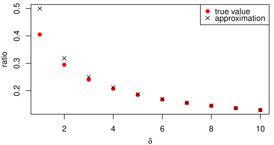
4. A counter example

Take $\mathcal{G}^{*}$ be the cycle of length 4 and $\mathcal{G}$ be the path of length 3. For both graphs, exact formulae for the normalising constants (when $D$ is the identity matrix) are known [7]:

$\displaystyle\mathscr{C}_{\mathcal{G}}(\delta,I_{4})$ $\displaystyle=$ $\displaystyle 2^{2\delta+3}\pi^{\frac{3}{2}}\Gamma\left(\frac{\delta+1}{2}\right)^{3}\Gamma\left(\frac{\delta}{2}\right),$
$\displaystyle\mathscr{C}_{\mathcal{G}^{*}}(\delta,I_{4})$ $\displaystyle=$ $\displaystyle 2^{2\delta+4}\dfrac{\pi^{2}\Gamma\left(\frac{\delta}{2}\right)\Gamma\left(\frac{\delta+1}{2}\right)\Gamma\left(\frac{\delta+2}{2}\right)^{3}}{\Gamma\left(\frac{\delta+3}{2}\right)}.$

Therefore, the correct ratio of the normalising constants is

(4) $$\dfrac{\mathscr{C}_{\mathcal{G}}(\delta,I_{4})}{\mathscr{C}_{\mathcal{G}^{*}}(\delta,I_{4})}=\dfrac{\Gamma\left(\frac{\delta+1}{2}\right)^{2}\Gamma\left(\frac{\delta+3}{2}\right)}{2\pi^{\frac{1}{2}}\Gamma\left(\frac{\delta+2}{2}\right)^{3}},$$

while the approximation from (1) is

(5) $$\dfrac{\mathscr{C}_{\mathcal{G}}(\delta,I_{4})}{\mathscr{C}_{\mathcal{G}^{*}}(\delta,I_{4})}\approx\dfrac{\Gamma\left(\frac{\delta}{2}\right)}{2\pi^{\frac{1}{2}}\Gamma\left(\frac{\delta+1}{2}\right)}.$$

By Stirling’s approximation, the relative error of the above approximation is

$\displaystyle\dfrac{\Gamma\left(\frac{\delta+2}{2}\right)^{3}\Gamma\left(\frac{\delta}{2}\right)}{\Gamma\left(\frac{\delta+1}{2}\right)^{3}\Gamma\left(\frac{\delta+3}{2}\right)}-1$ $\displaystyle=$ $\displaystyle\left(1+\dfrac{1}{4\delta}+\dfrac{1}{32\delta^{2}}\right)^{3}\left(1-\dfrac{3}{4\delta}+\dfrac{25}{32\delta^{2}}\right)(1+O(\delta^{-3}))^{4}-1$
$\displaystyle\sim$ $\displaystyle\dfrac{1}{2\delta^{2}},\quad\text{ as }\delta\to\infty.$

Therefore the error tends to zero as $\delta$ grows. Moreover, the first-order terms cancel so that the error decreases rapidly for increasing $\delta$. Figure 1 compares the ratios for small values of $\delta$.

Refer to caption
Figure 1. For the first ten positive integers $\delta$, we compare the correct ratio from Equation (4) and the approximation of Equation (5).

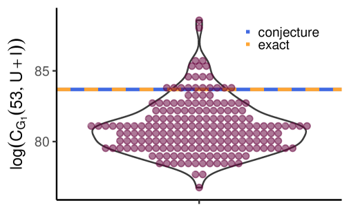
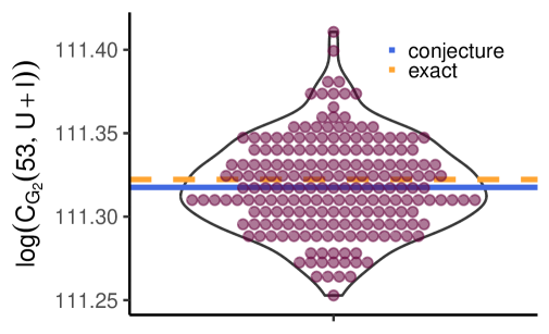
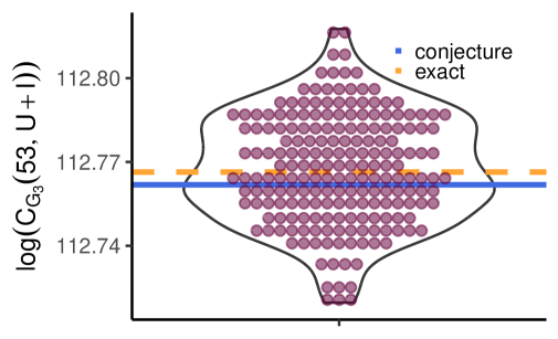
In the context of Bayesian inference, we need to compute the normalising constant $\mathscr{C}_{\mathcal{G}}(\delta+N,U+D)$, where $N$ is the number of data points, $U$ is the scatter matrix of the dataset, $\delta$ and $D$ are parameters of the prior distribution, often taken to be 3 and the identity matrix respectively. Since the parameter of the normalising constant in the posterior is $(\delta+N)$, with reasonable amounts of data this parameter will accordingly be quite large, and hence we may be in a regime where the approximation implied by Conjecture 1 is quite accurate.

As illustration, we use Fisher’s Iris Virginica dataset, which contains 4 variables (SL, SW, PL, PW) and 50 data points. There are three non-chordal graphs, as shown in Figure 2(a). In [3], we derived a new way to write the normalising constant $\mathscr{C}_{\mathcal{G}}(53,U+I)$ of these graphs as a one-dimensional integral, which can be computed numerically. For each of these three graphs, we compare this value and the conjectured value in Table 1. Further, we also compare with values obtained by Monte Carlo integration [4] in Figure 2(b). It can be seen that Roverato’s conjecture provides a very good estimate of the normalising constant, especially compared to the stochastic noise of the Monte Carlo integration.

$SL$ $SW$ $PL$ $PW$
$SL$ $SW$ $PL$ $PW$
$SL$ $SW$ $PL$ $PW$
(a)
Refer to caption
Refer to caption
Refer to caption
(b)
Figure 2. (a) The graphs $\mathcal{G}_{1}$, $\mathcal{G}_{2}$, $\mathcal{G}_{3}$ (from left to right), are the non-chordal graphs for Fisher’s Iris Virginica dataset. (b) Violin plots of the estimates of the values of $\log(\mathscr{C}_{\mathcal{G}_{j}}(53,U+I_{4}))$, where $j=1,2,3$, using Monte Carlo integration [4, 5] with $1000$ samples and for 200 different seeds. The horizontal lines represent the values obtained using Roverato’s conjecture and the exact one-dimensional integral in [3].
Table 1. The estimated values of $\log(\mathscr{C}_{\mathcal{G}_{j}}(53,U+I_{4}))$, for $j=1,2,3$. The graphs are displayed in Figure 2(a).
$\log(\mathscr{C}_{\mathcal{G}_{1}}(53,U+I_{4}))$ $\log(\mathscr{C}_{\mathcal{G}_{2}}(53,U+I_{4}))$ $\log(\mathscr{C}_{\mathcal{G}_{3}}(53,U+I_{4}))$
exact value [3] $83.6851$ $111.3223$ $112.7664$
conjectured value $83.6836$ $111.3175$ $112.7618$

5. Conclusions

While efficient to compute for $\mathcal{G}$-Wishart normalising constants, Roverato’s conjecture does not hold for all graphs. Instead we showed that the conjecture implies an approximation that had previously been employed in Bayesian samplers to speed up inference when computing the ratio of normalising constants with identity scale matrices [6]. In Bayesian inference the parameter of the normalising constant is increased by the amount of data, so that although not exact, Roverato’s conjecture may still offer a good approximation for general data matrices. If we view the conjecture as capturing the leading order term in some expansion, a key task is to understand the next-order terms; both whether they vanish quickly as in our simple counter-example, and whether they can also be expressed in terms of functions that are invariant of the data matrix like the conjecture itself. As such, the problem of whether the $\mathcal{G}$-Wishart normalising constant $\mathscr{C}_{\mathcal{G}}(\delta,D)$ can be expressed in terms of $\mathscr{C}_{\mathcal{G}}(\delta,I_{|\mathcal{V}(\mathcal{G})|})$ remains open.

Acknowledgements

The authors are grateful for funding support for this work from the University of Basel through the Research Fund for Excellent Junior Researchers (to CW).

References

  • [1] Alberto Roverato. Hyper inverse Wishart distribution for non-decomposable graphs and its application to Bayesian inference for Gaussian graphical models. Scandinavian Journal of Statistics, 29:391–411, 2002.
  • [2] A. P. Dawid and S. L. Lauritzen. Hyper-Markov laws in the statistical analysis of decomposable graphical models. Annals of Statistics, 21:1272–1317, 1993.
  • [3] Ching Wong, Giusi Moffa, and Jack Kuipers. A new way to evaluate G-Wishart normalising constants via Fourier analysis. 2024. arXiv:2404.06803.
  • [4] Aliye Atay-Kayis and Hélène Massam. A Monte Carlo method for computing the marginal likelihood in nondecomposable Gaussian graphical models. Biometrika, 92:317–335, 2005.
  • [5] Reza Mohammadi and Ernst C. Wit. BDgraph: An R package for Bayesian structure learning in graphical models. Journal of Statistical Software, 89:1–30, 2019.
  • [6] Reza Mohammadi, Hélène Massam, and Gérard Letac. Accelerating Bayesian structure learning in sparse Gaussian graphical models. Journal of the American Statistical Association, 118:1345–1358, 2023.
  • [7] Caroline Uhler, Alex Lenkoski, and Donald Richards. Exact formulas for the normalizing constants of Wishart distributions for graphical models. Annals of Statistics, 46:90–118, 2018.
  • [8] A. Mohammadi and E. C. Wit. Bayesian structure learning in sparse Gaussian graphical models. Bayesian Analysis, 10:109 – 138, 2015.
  • [9] Willem van den Boom, Alexandros Beskos, and Maria De Iorio. The G-Wishart weighted proposal algorithm: Efficient posterior computation for Gaussian graphical models. Journal of Computational and Graphical Statistics, 31:1215–1224, 2022.
  • [10] Alex Lenkoski. A direct sampler for G-Wishart variates. Stat, 2:119–128, 2013.
  • [11] Terence P. Speed and Harri T. Kiiveri. Gaussian Markov distributions over finite graphs. The Annals of Statistics, 14:138–150, 1986.
  • [12] Robert Grone, Charles R. Johnson, Eduardo M. de Sá, and Henry Wolkowicz. Positive definite completions of partial Hermitian matrices. Linear Algebra and its Applications, 58:109–124, 1984.
  • [13] Alberto Roverato and Joe Whittaker. The Isserlis matrix and its application to non-decomposable graphical Gaussian models. Biometrika, 85:711–725, 1998.