An entropy penalized approach for stochastic optimization with marginal law constraints. Complete version

Abstract

This paper focuses on stochastic optimal control problems with constraints in law, which are rewritten as optimization (minimization) of probability measures problem on the canonical space. We introduce a penalized version of this type of problems by splitting the optimization variable and adding an entropic penalization term. We prove that this penalized version constitutes a good approximation of the original control problem and we provide an alternating procedure which converges, under a so called Stability Condition, to an approximate solution of the original problem. We extend the approach introduced in a previous paper of the same authors including a jump dynamics, non-convex costs and constraints on the marginal laws of the controlled process. The interest of our approach is illustrated by numerical simulations related to demand-side management problems arising in power systems.

Key words and phrases: Stochastic control; optimization; Donsker-Varadhan representation; exponential twist; relative entropy; target law; demand-side management.

2020 AMS-classification: 49M99; 49J99; 60H10; 60J60; 65C05.

1 Introduction

Stochastic optimal control problems with constraints in law have constituted a very active field of research during the recent years. For instance [13, 43, 16, 17] treat expectation constraints. Other references prescribe marginal laws constraints, related for example to optimal transport [40, 47, 2, 20] or to the Schrödinger Bridge problems [37, 41]. They offer both theoretical and practical perspectives. On a theoretical point of view, (semi)martingale optimal transport and the Schrödinger bridge problem can be seen as stochastic versions of the classical optimal transport problem [11, 37, 19, 42].

On a practical point of view, expectation constraints are used for instance in demand side management applications in power system, typically to control the smart charging of a fleet of electrical vehicles while ensuring a minimum expected charge level for the batteries at the end of each day [44, 45]. In financial applications, the martingale optimal transport formulation introduced in [2] in the discrete time setting and in [40, 47] for the continuous time setting provides powerful tools to study model-free hedging of derivatives [2, 20]. As for the Schrödinger bridge, it is used for instance to estimate a model interpolating two sampled distributions [41] or to generate synthetic data [18, 26] that can be used to train neural networks.

In this paper we are interested in optimization problems of the form

$$J^{*}:=\inf_{{\mathbb{P}}\in{\cal K}\cap{\cal P}_{\mathbb{U}}(\eta_{0})}J({\mathbb{P}})\quad\text{with}\quad J({\mathbb{P}}):={\mathbb{E}}^{\mathbb{P}}\left[\int_{0}^{T}f(r,X_{r},\nu_{r}^{\mathbb{P}})dr+g(X_{T})\right],$$ (1.1)

precisely described in Section 3.1. More specifically, ${\cal K}$ is a convex subset of the space of probability measures on ${\cal P}(\Omega)$, where $\Omega=D([0,T],{\mathbb{R}}^{d})$ will be the canonical space of càdlàg trajectories with values in ${\mathbb{R}}^{d}$ equipped with the Skorohod metric. $\eta_{0}$ will be a given initial Borel probability on ${\mathbb{R}}^{d}$, $\mathbb{U}$ will be a closed subset of ${\mathbb{R}}^{p}$ for some $p\in{\mathbb{N}}^{*}$. ${\cal P}_{\mathbb{U}}(\eta_{0})$ is a subset of ${\cal P}(\Omega)$ defined in Definition 3.2 such that under ${\mathbb{P}}\in{\cal P}_{\mathbb{U}}(\eta_{0})$, the canonical process $X$ decomposes as

$$\left\{\begin{aligned} &X_{t}=X_{0}+\int_{0}^{t}b(r,X_{r},\nu_{r}^{\mathbb{P}})dr+\int_{0}^{t}\sigma(r,X_{r})dB_{r}+\left(q{\mathds{1}}_{\{|q|>1\}}\right)*\mu^{X}_{t}+\left(q{\mathds{1}}_{\{|q|\leq 1\}}\right)*(\mu^{X}-\mu^{L})_{t}\\ &X_{0}\sim\eta_{0},\end{aligned}\right.$$

where $\nu^{\mathbb{P}}:[0,T]\times\Omega\rightarrow\mathbb{U}$ is a progressively measurable process. $\mu^{X}$ is the jump measure of $X$ and $\mu^{L}=dtL(t,X_{t},dq)$ its ${\mathbb{P}}$-compensator characterized by the Lévy kernel $L$ (see Definition 2.2) and $B$ is a ${\mathbb{P}}$-Brownian motion. Problem (1.1) differs from a classical stochastic optimal control problem (in the weak formulation) in that it includes an additional constraint ${\mathbb{P}}\in{\cal K}$. Indeed, when ${\cal K}={\cal P}(\Omega)$, (1.1) is a stochastic control problem where only the drift is controlled, while the volatility and the jump intensity are left unchanged. When ${\cal K}\subset{\cal P}(\Omega)$, the formulation (1.1) recovers many types of aforementioned stochastic control problems with constraints in law. For example, when ${\cal K}=\left\{{\mathbb{P}}\in{\cal P}(\Omega)~:~{\mathbb{P}}_{T}=\eta_{T}\right\}$ for some prescribed terminal distribution $\eta_{T}\in{\cal P}({\mathbb{R}}^{d})$, Problem (1.1) can be interpreted as a optimal transport problem in the spirit of [40, 47]. In the more specific case where $L=0$, $b(t,x,u)=u$, $\sigma(t,x)=I_{d}$, $g=0$ and $f(t,x,u)=\frac{1}{2}|u|^{2}$, Problem (1.1) comes down to a Schrödinger bridge problem, see e.g. [37].

We discuss now our methodology which extends the techniques developed in previous paper [6]. Indeed, in that paper, we considered stochastic control problems of the form (1.1) in the case ${\cal K}={\cal P}(\Omega)$, $\eta_{0}$ is deterministic and $L=0$, i.e. continuous trajectories case. Thereby, we introduced a penalized version of that problem by splitting the decision variables and by adding a relative entropy divergence. Following this approach, we propose in this article to approximate Problem (1.1) by considering the entropy penalized formulation

$${\cal J}_{\epsilon}^{*}:=\inf_{({\mathbb{P}},\mathbb{Q})\in{\cal A}}{\cal J}_{\epsilon}(\mathbb{Q},{\mathbb{P}})\quad\text{with}\quad{\cal J}_{\epsilon}(\mathbb{Q},{\mathbb{P}}):={\mathbb{E}}^{\mathbb{Q}}\left[\int_{0}^{T}f(r,X_{r},\nu_{r}^{\mathbb{P}})dr+g(X_{T})\right]+\frac{1}{\epsilon}H(\mathbb{Q}|{\mathbb{P}}),$$ (1.2)

where ${\cal A}$ is a subset of ${\cal P}_{\mathbb{U}}(\eta_{0})\times{\cal K}$ (see Definition 3.10), $H$ is the relative entropy (see Definition 2.3), and $\epsilon>0$ is a penalization parameter intended to go to $0$ in order to impose $\mathbb{Q}={\mathbb{P}}$. The advantage of the penalized version (1.2) is that it allows to distribute the constraint ${\cal K}\cap{\cal P}_{\mathbb{U}}(\eta_{0})$ in (1.1) either on ${\mathbb{P}}$ or $\mathbb{Q}$ by considering an alternating minimization method leading to two subproblems

$$\underset{{\mathbb{P}}\in{\cal P}_{\mathbb{U}}(\eta_{0})}{\inf}~{\cal J}_{\epsilon}(\mathbb{Q},{\mathbb{P}})\quad\text{and}\quad\underset{\mathbb{Q}\in{\cal K}}{\inf}~{\cal J}_{\epsilon}(\mathbb{Q},{\mathbb{P}}),$$ (1.3)

that are easier to solve. For example when ${\cal K}=\left\{{\mathbb{P}}\in{\cal P}(\Omega)~:~{\mathbb{P}}_{T}=\eta_{T}\right\}$, the constraint on the initial law and the dynamics is supported by the variable ${\mathbb{P}}\in{\cal P}_{\mathbb{U}}(\eta_{0})$, whereas the constraint ${\mathbb{P}}_{T}=\eta_{T}$ is reported on $\mathbb{Q}$ by imposing $\mathbb{Q}_{T}\in{\cal K}$.

The contribution of the present paper is twofold. First we prove that the entropy penalized formulation (1.2) indeed approximates the original Problem (1.1) in a sense to be specified, when $\epsilon$ vanishes, see Proposition 3.15. Second, taking advantage of the simplicity of each subproblem (1.3), we propose an alternating algorithm producing a sequence of iterates (by updating alternatively the variables ${\mathbb{P}}$ and $\mathbb{Q}$) which is proved to provide a good approximate solution of Problem (1.2), when the number of iterations is sufficiently large. We emphasize that the present paper extends [6] in several directions. First we consider the case of jump (instead of continuous) diffusions. Second, as already mentioned, we take into account additional constraints by introducing the subset ${\cal K}$, including the case of a prescribed terminal distribution. Third, we are able to deal with non-convex running cost w.r.t. the control variable by the introduction of a (so called) Mixed Variational Inequality (MVI) assumption on $f$, $b$ and $\mathbb{U}$, similarly to [34, 29, 25]. The proofs of our results follow the same lines as [6], but raise additional technical difficulties, mainly due to the presence of jumps in the dynamics and to the MVI assumption.

We now present a short overview of the literature to solve Problem (1.1) in some particular cases. In the case ${\cal K}=\left\{{\mathbb{P}}\in{\cal P}(\Omega)|{\mathbb{P}}_{T}=\eta_{T}\right\}$, [40, 47, 37] rely on Lagrangian dualization techniques. Under some general conditions, the solutions of Problem (1.1) are characterized by two Lagrange multipliers which verify a coupled system of non-linear differential equations, which is Hamilton-Jacobi-Bellman (HJB) equations in [40, 47] or a Schrödinger system in [37, 12]. In [47], the HJB characterization of the solution of optimal transport problems naturally leads to finite difference schemes method, which are very reminiscent of an algorithm to solve mass transport problem introduced in [3], whereas the solution to Schrödinger system can be approximated using the so called Iterative Proportional Fitting Procedure, also referred to as Sinkhorn algorithm [23, 19, 10].

When considering expectation constraints corresponding to the case
${\cal K}=\{{\mathbb{P}}\in{\cal P}(\Omega)~:~{\mathbb{E}}^{\mathbb{P}}[\psi(X_{T})]\leq 0\},$ for some measurable function $\psi$, two types of approaches have been proposed in the literature. In [16, 17], the author considers the Markovian setting and uses a constraint penalization technique to prove that the solution to Problem (1.1) is characterized by a coupled Hamilton-Jacobi-Bellman system on the space of measures. In [43], the authors treat a non-Markovian setting by a Lagrangian dualization approach. Deep-learning schemes have also been developed to tackle Problem (1.1) with very general constraints set ${\cal K}$ in [24]. They extend to the mean-field setting an exact penalization approach developed in [5] to solve stochastic control problems with state constraints by introducing a stochastic target problem. To this aim they consider a linear-convex model where the controlled process follows a linear dynamics without jumps ($L=0$) and the cost is convex. Similarly to those techniques, our approach is based on a penalization method. However, the originality of our approach relies on the fact that we split the decision variable into two variables and introduce the penalization in order to force those two variables to be close.

The paper is organized as follows. Section 3 is concerned with the analysis of the entropy penalized formulation (1.2). In Proposition 3.15 we prove that Problem (1.2) constitutes a good approximation of Problem (1.1) in the sense of Definition 3.13. In Section 4 we propose an alternating minimization procedure to compute a minimizing sequence $({\mathbb{P}}^{k},\mathbb{Q}^{k})_{k\geq 1}$ to Problem (1.2) and prove the convergence of the iterates $({\cal J}_{\epsilon}(\mathbb{Q}^{k},{\mathbb{P}}^{k}))_{k\geq 1}$ to the optimal value ${\cal J}^{*}$ under a suitable Stability Condition 4.5, which will be related to natural assumptions on Problem 1.1. We introduce in particular Hypothesis 4.2 on the running cost $f$ and the admissible set of controls $\mathbb{U}$ allowing to alleviate standard convexity assumptions to prove the convergence of the sequence of the iterates $({\cal J}_{\epsilon}(\mathbb{Q}^{k},{\mathbb{P}}^{k}))_{k\geq 1}$. More specifically, Hypothesis 4.2 only requires the existence of a solution to a MVI allowing to tackle some non-convex settings. In Section 5 we provide several examples showing that the method developed in Section 4 has a wide range of applications. In a first example we treat the case of stochastic optimal control with jumps with some settings where the cost function $f$ is not convex in the control variable $u$, see Theorem 5.12. In a second example, see Theorem 5.14, we focus on the case where we prescribe the terminal distribution of the state process in the framework of continuous diffusions ($L=0$). Finally in Section 6, numerical simulations illustrate the interest of our approach to deal with demand side management problems arising in power systems.

2 Notations, definitions and classical results

• All vectors $x\in{\mathbb{R}}^{d}$ are column vectors. Given $x\in{\mathbb{R}}^{d}$, $|x|$ will denote its Euclidean norm.

• Given a matrix $A\in{\mathbb{R}}^{d\times d}$, $\|A\|:=\sqrt{Tr[AA^{\top}]}$ will denote its Frobenius norm.

• $S({\mathbb{R}}^{d})$ (resp. $S^{+}({\mathbb{R}}^{d}),S^{++}({\mathbb{R}}^{d})$) will denote the space of symmetric (resp. positive definite, strictly positive definite) matrices on ${\mathbb{R}}^{d}$.

• For any $x\in{\mathbb{R}}^{d}$, $\delta_{x}$ will denote the Dirac mass in $x$.

• The function $x\mapsto x\log(x)$ defined on $]0;+\infty[$ will be extended (without further mention) to $x=0$ by continuity.

• $\mathbb{U}$ will denote a closed subset of ${\mathbb{R}}^{p}$ where $p\in{\mathbb{N}}^{*}$.

• Given a measurable space $(E,{\cal E})$, ${\cal P}(E)$ will denote the set of probability measures ${\mathbb{P}}$ on ${\cal E}$.

• Equality between stochastic processes on some probability space are in the sense of indistinguishability.

• Given $0\leq t\leq T$, $D([t,T],{\mathbb{R}}^{d})$ will denote of càdlàg functions defined on $[t,T]$ with values in ${\mathbb{R}}^{d}$. In the whole paper $\Omega$ will denote space $D([0,T],{\mathbb{R}}^{d})$. For any $t\in[0,T]$ we denote by $X_{t}:\omega\in\Omega\mapsto\omega_{t}$ the coordinate mapping on $\Omega.$ We introduce the $\sigma$-field ${\cal F}:=\sigma(X_{r},0\leq r\leq T)$. On the measurable space $(\Omega,{\cal F}),$ we introduce the canonical process $X:\omega\in([0,T]\times\Omega,{\cal B}([0,T])\otimes{\cal F})\mapsto X_{t}(\omega)=\omega_{t}\in({\mathbb{R}}^{d},{\cal B}({\mathbb{R}}^{d}))$.

  We endow $(\Omega,{\cal F})$ with the right-continuous filtration ${\cal F}_{t}:=\underset{t<s<T}{\bigcap}\sigma(X_{r},t\leq r\leq T).$ The filtered space $(\Omega,{\cal F},({\cal F}_{t}))$ will be called the canonical space (for the sake of brevity, we denote $({\cal F}_{t})_{t\in[0,T]}$ by $({\cal F}_{t})$).

• ${\cal K}$ will denote a convex subset of ${\cal P}(\Omega)$.

• ${\cal P}_{pred}$ will denote the predictable $\sigma$-algebra of $\Omega\times[0,T]$ with respect to the filtration $({\cal F}_{t})_{t\in[0,T]})$. We also set $\tilde{\cal P}:={\cal P}_{pred}\otimes{\cal B}({\mathbb{R}}^{d})$.

• Given ${\mathbb{P}}\in{\cal P}(\Omega)$ and $t\in[0,T]$, ${\mathbb{P}}_{t}$ will denote the marginal at time $t$ of ${\mathbb{P}}$, that is the law of $X_{t}$ under ${\mathbb{P}}$.

• Given an $({\mathbb{P}},{\cal F}_{t})$-local martingale $M$ for ${\mathbb{P}}\in{\cal P}(\Omega)$, $[M]$ will denote its quadratic variation. If moreover $M$ is locally square integrable under ${\mathbb{P}}$, $\langle M\rangle$ will denote its predictable quadratic variation. Note that if $M$ is continuous, $[M]=\langle M\rangle$.

• Given a progressively measurable process $Y$ and a stopping time $\tau$, $Y^{\tau}$ will denote the stopped process $Y_{\cdot\wedge\tau}$. If ${\mathbb{P}}$ is a probability measure on $(\Omega,{\cal F})$, ${\mathbb{P}}^{\tau}$ will denote the restriction of ${\mathbb{P}}$ to ${\cal F}_{\tau}$.

• Given a probability measure ${\mathbb{P}}$ on $(\Omega,{\cal F})$, ${\cal A}_{loc}^{+}({\mathbb{P}})$ will denote the space of real-valued càdlàg adapted process $A$ with non-decreasing path and locally integrable variation.

• Throughout the paper we will use the notion of random measures and their associated compensator. For a detailed discussion on this topic as well as some unexplained notations we refer to Chapter II and Chapter III in [32]. In particular, the compensator of a random measure is introduced in Theorem 1.8, Chapter II in [32].

• Given an integer-valued random measure $\mu$ and a probability measure ${\mathbb{P}}$ on $(\Omega,{\cal F})$, ${\cal G}_{loc}^{\mathbb{P}}(\mu)$ will denote the set of $\tilde{\cal P}$-measurable functions for which a stochastic integral can be defined in the sense of Definition 1.27, Chapter II of [32].

• Also, given an integer-valued random measure $\mu$ and a $\tilde{\cal P}$-measurable function $W:[0,T]\times\Omega\times{\mathbb{R}}^{d}\rightarrow{\mathbb{R}}$, we denote $W*\mu:=\int_{]0,\cdot]\times{\mathbb{R}}^{d}}W(r,X,q)\mu(drdq)$ (when it exists) the integral of $W$ with respect to (w.r.t.) $\mu$.

• Given a probability measure ${\mathbb{P}}\in{\cal P}(\Omega)$ and an integer random measure $\mu$ with compensator $\tilde{\mu}$, ${\cal G}_{loc}^{\mathbb{P}}(\mu)$ will denote the set of $\tilde{\cal P}$-measurable function $W$ such that the stochastic integral $W*(\mu-\tilde{\mu})$ w.r.t. the compensated measure $\mu-\tilde{\mu}$ is well-defined.

Definition 2.1.

(Stochastic interval). Let $\tau$ be a stopping time. We set $\llbracket 0,\tau\rrbracket:=\{(t,\omega)\in[0,T]\times\Omega~:~0\leq t\leq\tau(\omega)\}.$

Definition 2.2.

(Lévy kernel). Let $L:[0,T]\times\Omega\times{\cal B}({\mathbb{R}}^{d})$ be a Borel function. We say that $L$ is a Lévy kernel if we have the following.

1. $L(t,X,.)$ is a $\sigma$-finite non-negative measure on ${\mathbb{R}}^{d}$ such that $L(t,X,\{0\})=0$.

2. $(t,X)\mapsto L(t,X,A)$ is predictable for all $A\in{\cal B}({\mathbb{R}}^{d})$.

3. $(t,X)\mapsto\int_{A}(1\wedge|q|^{2})L(t,X,dq)$ is Borel and bounded for all $A\in{\cal B}({\mathbb{R}}^{d})$.

Definition 2.3.

(Relative entropy). Let ${\mathbb{P}},\mathbb{Q}$ be two elements of ${\cal P}(\Omega)$. The relative entropy $H(\mathbb{Q}|{\mathbb{P}})$ of $\mathbb{Q}$ with respect to ${\mathbb{P}}$ is given by

$$\left\{\begin{aligned} &{\mathbb{E}}^{\mathbb{Q}}\left[\log\frac{d\mathbb{Q}}{d{\mathbb{P}}}\right]&\text{if}\quad\mathbb{Q}\ll{\mathbb{P}}\\ &+\infty&\text{otherwise.}\end{aligned}\right.$$

Remark 2.4.

1. Let ${\mathbb{P}},\mathbb{Q}\in{\cal P}(\Omega)$ such that $\mathbb{Q}\ll{\mathbb{P}}$. Since $t\in[0,1]\mapsto-t\log(t)$ is bounded by $1/e$, the entropy

   $$H(\mathbb{Q}|{\mathbb{P}})=\int_{\Omega}\frac{d\mathbb{Q}}{d{\mathbb{P}}}\log\frac{d\mathbb{Q}}{d{\mathbb{P}}}{\mathbb{P}}(d\omega)={\mathbb{E}}^{\mathbb{Q}}\left[\log\frac{d\mathbb{Q}}{d{\mathbb{P}}}\right],$$

   is well-defined, strictly greater than $-\infty$. In fact it is even always non-negative by Jensen’s inequality, the function $x\mapsto x\log(x)$ being convex on ${\mathbb{R}}_{+}$. It could be $+\infty$.

2. The relative entropy $H$ is non-negative and jointly strictly convex, that is for all ${\mathbb{P}}_{1},{\mathbb{P}}_{2},\mathbb{Q}_{1},\mathbb{Q}_{2}\in{\cal P}(E)$, for all $\lambda\in]0,1[$, $H(\lambda\mathbb{Q}_{1}+(1-\lambda)\mathbb{Q}_{2}|\lambda{\mathbb{P}}_{1}+(1-\lambda){\mathbb{P}}_{2})<\lambda H(\mathbb{Q}_{1}|{\mathbb{P}}_{1})+(1-\lambda)H(\mathbb{Q}_{2}|{\mathbb{P}}_{2})$. Moreover, $({\mathbb{P}},\mathbb{Q})\mapsto H(\mathbb{Q}|{\mathbb{P}})$ is lower semicontinuous with respect to the weak convergence of ${\cal P}(E)$, which corresponds to the weak* convergence on Polish spaces. We refer to Lemma 1.4.3 in [22] for a proof of those properties.

3. Let ${\mathbb{P}},\mathbb{Q}\in{\cal P}(\Omega)$ and let $t\in[0,T]$. Lemma 2.3 in [21] applied with ${\cal F}_{2}={\cal F}$ and ${\cal F}_{1}=\sigma(X_{t})$ yields $H(\mathbb{Q}_{t}|{\mathbb{P}}_{t})\leq H(\mathbb{Q}|{\mathbb{P}})$.

Definition 2.5.

(Markovian probability measure). A probability measure ${\mathbb{P}}$ is said to be Markovian if for all $t\in[0,T]$, for all $F\in{\cal B}_{b}(C([t,T],{\mathbb{R}}^{d}),{\mathbb{R}})$,

$${\mathbb{E}}^{\mathbb{P}}\left[F\left(\left(X_{r}\right)_{r\in[t,T]}\right)\middle|{\cal F}_{t}\right]={\mathbb{E}}^{\mathbb{P}}\left[F\left(\left(X_{r}\right)_{r\in[t,T]}\right)\middle|X_{t}\right].$$ (2.1)

The result below is Proposition 3.68, Chapter III in [31].

Proposition 2.6.

Let ${\mathbb{P}}\in{\cal P}(\Omega)$. Let $\mu$ be a random measure with ${\mathbb{P}}$-compensator $\mu^{L}:=dtL(t,X,dq),$ where $L$ is a Lévy kernel in the sense of Definition 2.2. Let $W$ be a $\tilde{\cal P}$-measurable function and let $b_{0}>0$. The following statements are equivalent.

1. $W\in{\cal G}_{loc}^{\mathbb{P}}(\mu)$.

2. $\left(W^{2}{\mathds{1}}_{\{|W|\leq b_{0}\}}+|W|{\mathds{1}}_{\{|W|>b_{0}\}}\right)*\mu^{L}\in{\cal A}_{loc}^{+}({\mathbb{P}})$.

Below we assume given two progressively measurable functions $b:[0,T]\times\Omega\rightarrow{\mathbb{R}}^{d}$ and $a:[0,T]\times\Omega\rightarrow S({\mathbb{R}}^{d})$ , as well as a Lévy kernel $L$ in the sense of Definition 2.2. $(b,a,L)$ represents a classical triplet of ”characteristics” in the sense of Jacod-Shiryaev, see Section 2, Chapter II in [32]. Let also $\eta_{0}\in{\cal P}({\mathbb{R}}^{d})$ .

Definition 2.7.

(Martingale problem). Given the triplet $(b,a,L)$, a probability measure ${\mathbb{P}}\in{\cal P}(\Omega)$ is called solution of the martingale problem with characteristics $(b,a,L)$ and with initial condition $\eta_{0}$ if under ${\mathbb{P}}$ the canonical process decomposes as

$$\left\{\begin{aligned} &X_{t}=X_{0}+\int_{0}^{t}b_{r}dr+M_{t}^{\mathbb{P}}+\left(q{\mathds{1}}_{\{|q|>1\}}\right)*\mu^{X}_{t}+\left(q{\mathds{1}}_{\{|q|\leq 1\}}\right)*(\mu^{X}-\mu^{L})_{t}\\ &X_{0}\sim\eta_{0},\end{aligned}\right.$$ (2.2)

where $M^{\mathbb{P}}$ is a continuous ${\mathbb{P}}$-local martingale verifying $[M^{\mathbb{P}}]=\int_{0}^{\cdot}a_{r}dr$.

Remark 2.8.

By classical stochastic calculus arguments, see e.g. Theorem 2.42, Chapter II in [32], we can state that the two following properties are equivalent.

1. ${\mathbb{P}}$ is solution to the martingale problem associated to $(b,a,L)$ with initial condition $\eta_{0}$.

2. We have $X_{0}\sim\eta_{0}$ under ${\mathbb{P}}$ and for all bounded functions $\phi\in{\cal C}^{1,2}$, the process $\phi(\cdot,X_{\cdot})-\phi(0,X_{0})-\int_{0}^{\cdot}{\cal L}(\phi)(r,X)dr$ is a ${\mathbb{P}}$-local martingale, where

   $${\cal L}(\phi)(t,X) =\partial_{t}\phi(t,X_{t})+\langle b(t,X),\nabla_{x}\phi(t,X_{t})\rangle+\frac{1}{2}Tr[\nabla_{x}^{2}\phi(t,X_{t})a(t,X)]$$ (2.3)

   $$+\int_{{\mathbb{R}}^{d}}\left(\phi(t,X_{t-}+q)-\phi(t,X_{t-})-{\mathds{1}}_{\{|q|\leq 1\}}\langle\nabla_{x}\phi(t,X_{t-}),q\rangle\right)L(t,X,dq).$$

The definition below postulates that, given a triplet of characteristics $(b,a,L)$ the ”martingale problem” with any initial condition at any time $s$ and trajectory position $\omega$ restricted to $[0,s]$ admits existence and measurability.

Definition 2.9.

(Flow existence property). We will say that a triplet of characteristics $(b,a,L)$ satisfies the flow existence property if there exists a kernel $({\mathbb{P}}^{s,\omega})_{(s,\omega)\in[0,T]\times\Omega}$ (path-dependent class) of elements of ${\cal P}(\Omega)$ verifying the following assertions.

1. For all $(s,\omega)\in[0,T]\times\Omega$, ${\mathbb{P}}^{s,\omega}(X_{r}=\omega_{r},0\leq r\leq s)=1$.

2. For all $(s,\omega)\in[0,T]\times\Omega$, under ${\mathbb{P}}^{s,\omega}$ the canonical process decomposes for all $t\in[s,T]$ as

   $$X_{t}=\omega_{s}+\int_{s}^{t}b_{r}dr+M^{s,\omega}_{t}+\left(q{\mathds{1}}_{\{|q|>1\}}\right)*\mu^{X}_{t}+\left(q{\mathds{1}}_{\{|q|\leq 1\}}\right)*(\mu^{X}-\mu^{L})_{t},$$ (2.4)

   where $M^{s,\omega}$ is a continuous ${\mathbb{P}}^{s,\omega}$-local martingale such that $[M^{s,\omega}]=\int_{s}^{\cdot}a_{r}dr$.

3. The function $(s,\omega)\in[0,T]\times\Omega\mapsto{\mathbb{P}}^{s,\omega}\in{\cal P}(\Omega)$ is progressively measurable in the sense that $(s,\omega)\mapsto{\mathbb{P}}^{s,\omega}(A)$ is progressively measurable for every $A\in{\cal F}$.

Definition 2.10.

(Minimizing sequence, solution and $\epsilon$-solution). Let $(Y,d)$ be a metric space. Let $J:Y\mapsto{\mathbb{R}}_{+}$ be a function. Let $Z\subset Y$. Let $J^{*}:=\underset{x\in Z}{\inf}J(x)$.

1. A minimizing sequence for $J$ is a sequence $(x_{n})_{n\geq 0}$ of elements of $Z$ such that $J(x_{n})\underset{n\rightarrow+\infty}{\longrightarrow}J^{*}$. We remark that $J^{*}$ is finite if and only if $Z$ is non empty.

2. We will say that $x^{*}\in Z$ is a solution to (or minimizer of) the optimization Problem

   $$\underset{x\in Z}{\inf}J(x),$$ (2.5)

   if $J(x^{*})=J^{*}.$ In this case, $J^{*}=\underset{x\in Z}{\min}J(x)$.

3. For $\epsilon\geq 0$, we will say that $x_{\epsilon}\in Z$ is an $\epsilon$-solution to the optimization Problem (2.5) if $0\leq J(x_{\epsilon})-J^{*}\leq\epsilon$. We also say that $x_{\epsilon}$ is $\epsilon$-optimal for the (optimization) Problem (2.5).

The following is Definition 17.1 in [1].

Definition 2.11.

(Correspondence and measurable selector).

1. A correspondence ${\cal T}$ from a set $S$ to a set $Y$ is an application $S\rightarrow 2^{Y}$.

2. Let $(S,{\mathscr{S}})$ and $(Y,{\cal Y})$ be two measurable spaces. Given a correspondence ${\cal T}$ from $S$ to $Y$, a measurable selector of ${\cal T}$ is a $({\mathscr{S}},{\cal Y})$-measurable map $m:S\rightarrow Y$ such that for all $s\in S$, $m(s)\in{\cal T}(s)$.

3 From the original problem to the penalized problem

In the rest of the paper, we fix a probability measure $\eta_{0}\in{\cal P}({\mathbb{R}}^{d})$.

In this section we formulate a minimization problem on the space of probability measures ${\cal P}(\Omega)$ and we introduce a regularized version of this problem by splitting the variables and adding a relative entropy penalization. We prove in Proposition 3.15 that the regularized problem approximates in some sense the original optimization program.

3.1 Description of the optimization problem on the space of probability measures

We will consider in the whole paper a (controlled) drift $b\in{\cal B}([0,T]\times{\mathbb{R}}^{d}\times\mathbb{U},{\mathbb{R}}^{d})$, a diffusion matrix $\sigma\in{\cal B}([0,T]\times{\mathbb{R}}^{d},{\mathbb{R}}^{d\times d})$ and a Lévy kernel $L$ in the sense of Definition 2.2. We assume in the rest of the paper that $\sigma\sigma^{\top}$ is invertible and we introduce the notation

$$\Sigma:=\sigma\sigma^{\top},\quad\sigma^{-1}:=\sigma^{\top}\Sigma^{-1},$$ (3.1)

$\sigma^{-1}$ being the generalized inverse of $\sigma$. For the moment we do not make any other assumption on these coefficients. For the rest of the article, we will denote

$$\mu^{L}(X_{t-},dt,dq):=L(t,X_{t-},dq)dt.$$ (3.2)

Later we will make use of the following assumption on the coefficients $b$ and $\sigma$.

Hypothesis 3.1.

(Bounded drift and ellipticity).

1. $b$ is bounded.

2. There exists $c_{\sigma}>0$ such that for all $(t,x)\in[0,T]\times{\mathbb{R}}^{d}$, $\xi\in{\mathbb{R}}^{d}$, $\xi^{\top}\Sigma(t,x)\xi\geq c_{\sigma}|\xi|^{2}.$

We now define the set of admissible dynamics ${\cal P}_{\mathbb{U}}(\eta_{0})$ for our optimization problem.

Definition 3.2.

(Admissible dynamics). A probability measure ${\mathbb{P}}$ is an element of ${\cal P}_{\mathbb{U}}(\eta_{0})$ if there exists a progressively measurable process $\nu^{\mathbb{P}}:[0,T]\times\Omega\rightarrow\mathbb{U}$ such that, under ${\mathbb{P}}$, the canonical process $X$ has decomposition

$$\left\{\begin{aligned} &X_{t}=X_{0}+\int_{0}^{t}b(r,X_{r},\nu_{r}^{\mathbb{P}})dr+M_{t}^{\mathbb{P}}+\left(q{\mathds{1}}_{\{|q|>1\}}\right)*\mu^{X}_{t}+\left(q{\mathds{1}}_{\{|q|\leq 1\}}\right)*(\mu^{X}-\mu^{L})_{t}\\ &X_{0}\sim\eta_{0},\end{aligned}\right.$$ (3.3)

where $M^{\mathbb{P}}$ is a continuous local martingale such that $[M^{\mathbb{P}}]=\int_{0}^{\cdot}\Sigma(r,X_{r})dr$ and $\mu^{L}(=\mu^{L,{\mathbb{P}}})$ is the ${\mathbb{P}}$-compensator of $\mu^{X}$ given by (3.2). If $\nu^{\mathbb{P}}_{t}=u^{\mathbb{P}}(t,X_{t})$ for a function $u^{\mathbb{P}}\in{\cal B}([0,T]\times{\mathbb{R}}^{d},\mathbb{U})$, we will denote ${\mathbb{P}}\in{\cal P}_{\mathbb{U}}^{Markov}(\eta_{0})$.

In the following, for any ${\mathbb{P}}\in{\cal P}_{\mathbb{U}}(\eta_{0})$, we will use the notation

$$b_{t}^{\mathbb{P}}:=b(t,X_{t},\nu_{t}^{\mathbb{P}}).$$ (3.4)

Remark 3.3.

Given a progressively measurable function $u:[0,T]\times\Omega\rightarrow\mathbb{U}$, setting $\nu^{\mathbb{P}}=u(\cdot,X)$, ${\mathbb{P}}$ is a solution to the martingale problem

$$\left\{\begin{aligned} &X_{t}=X_{0}+\int_{0}^{t}b(r,X_{r},u(r,X))dr+M_{t}^{\mathbb{P}}+\left(q{\mathds{1}}_{\{|q|>1\}}\right)*\mu^{X}_{t}+\left(q{\mathds{1}}_{\{|q|\leq 1\}}\right)*(\mu^{X}-\mu^{L})_{t}\\ &X_{0}\sim\eta_{0},\end{aligned}\right.$$ (3.5)

where $M^{\mathbb{P}}$ is a continuous local martingale such that $[M^{\mathbb{P}}]=\int_{0}^{\cdot}\Sigma(r,X_{r})dr$ and $\mu^{L}$ is given by (3.2).

• In particular ${\mathbb{P}}$ is a solution to the martingale problem in the sense of Definition 2.7 with characteristics $(b(t,X_{t},u(t,X)),\Sigma(t,X_{t}),L)$.

• If given $u$ there is only one probability measure ${\mathbb{P}}$ such that ${\mathbb{P}}$ is a solution of previous martingale problem we will write ${\mathbb{P}}={\mathbb{P}}^{u}$.

We also define a running (resp. terminal) cost $f\in{\cal B}([0,T]\times{\mathbb{R}}^{d}\times\mathbb{U},{\mathbb{R}})$ (resp. $g\in{\cal B}({\mathbb{R}}^{d},{\mathbb{R}})$), which satisfy the following assumption.

Hypothesis 3.4.

(Running and terminal costs).

1. $f,g\geq 0$.

2. $f,g$ are bounded.

Remark 3.5.

1. From now on, for simplicity of the exposition we will set $g=0$.

2. Hypothesis 3.4 item 2 could be replaced by a polynomial growth assumption on $f$ but this would require strong regularity of the Lévy kernel $L$. It would be difficult to ensure the existence of a probability measure ${\mathbb{P}}\in{\cal P}_{\mathbb{U}}(\eta_{0})$ such that $J({\mathbb{P}})<+\infty$, where $J$ was defined in (1.1), without the existence of moments for $X$ under ${\mathbb{P}}$. We chose to have bounded costs in order to consider more complex dynamics.

We are interested in the optimization Problem (1.1) on the space of probability measures. Recall that the admissible set is of the form ${\cal P}_{\mathbb{U}}(\eta_{0})\cap{\cal K}$, where ${\cal K}$ is a convex subset of ${\cal P}(\Omega)$.

Remark 3.6.

Typical examples of ${\cal K}$ include the following.

1. ${\cal K}={\cal P}(\Omega)$.

2. ${\cal K}=\left\{\mathbb{Q}\in{\cal P}(\Omega)~:~{\mathbb{E}}^{\mathbb{Q}}\left[\psi(X_{T})\right]\leq 0\right\}$, for some $\psi\in{\cal B}({\mathbb{R}}^{d},{\mathbb{R}})$.

3. ${\cal K}=\left\{\mathbb{Q}\in{\cal P}(\Omega)~:~\mathbb{Q}_{T}=\eta_{T}\right\}$ for a fixed $\eta_{T}\in{\cal P}({\mathbb{R}}^{d})$.

We will examine in detail the cases related to $1.$ and $3.$ in Section 5 and provide numerical simulations for $3.$ in Section 6.

Remark 3.7.

1. The formulation (1.1) allows to deal with problems falling outside the classical framework of the stochastic optimal control, which corresponds to ${\cal K}={\cal P}(\Omega)$, see item 1.

2. The optimization problem (1.1) with ${\cal K}={\cal P}(\Omega)$, without jumps and with convex costs was the object of [6].

The admissible set ${\cal K}\cap{\cal P}_{\mathbb{U}}(\eta_{0})$ can a priori be empty. In this case $J^{*}=+\infty$ and Problem (1.1) has no interest. We will then often assume the following.

Hypothesis 3.8.

(Feasibility). ${\cal K}\cap{\cal P}_{\mathbb{U}}(\eta_{0})\neq\emptyset$.

Remark 3.9.

Assume Hypotheses 3.4 and 3.8. Then $J^{*}<+\infty$. Indeed, $f$ being bounded, we have $J^{*}\leq J({\mathbb{P}})<\infty$, for every ${\mathbb{P}}\in{\cal P}_{\mathbb{U}}(\eta_{0})\cap{\cal K}$.

3.2 Entropic penalization

We formulate an approximation of Problem (1.1) by doubling the optimization variables and adding a relative entropy penalization. We therefore obtain Problem (1.2), where $\epsilon>0$ is the penalization parameter and the admissible set ${\cal A}$ is the subset of ${\cal P}(\Omega)^{2}$ defined below.

Definition 3.10.

(Regularized set). Let ${\cal A}$ be the subset of probability measures $({\mathbb{P}},\mathbb{Q})\in{\cal P}(\Omega)^{2}$ such that

1. ${\mathbb{P}}\in{\cal P}_{\mathbb{U}}(\eta_{0})$ and $\mathbb{Q}\in{\cal K}$.

2. $H(\mathbb{Q}|{\mathbb{P}})<+\infty$.

We can characterize the elements of the set ${\cal A}$ in terms of the decomposition of the canonical process $X$.

Lemma 3.11.

Let $({\mathbb{P}},\mathbb{Q})\in{\cal A}$. We have the following properties.

1. Under ${\mathbb{P}}$ the canonical process decomposes as (3.3), and, under $\mathbb{Q}$, the canonical process decomposes as

   $$X_{t}=X_{0}+\int_{0}^{t}\beta^{\mathbb{Q}}_{r}dr+\left(q{\mathds{1}}_{\{|q|\leq 1\}}(Y^{\mathbb{Q}}-1)\right)*\mu^{L}_{t}+M_{t}^{\mathbb{Q}}+\left(q{\mathds{1}}_{\{|q|>1\}}\right)*\mu^{X}_{t}+\left(q{\mathds{1}}_{\{|q|\leq 1\}}\right)*(\mu^{X}-Y^{\mathbb{Q}}.\mu^{L})_{t},$$ (3.6)

   where $\beta^{\mathbb{Q}}:[0,T]\times\Omega\rightarrow{\mathbb{R}}^{d}$ is a progressively measurable function, $Y^{\mathbb{Q}}:[0,T]\times\Omega\times{\mathbb{R}}^{d}\rightarrow{\mathbb{R}}^{+}$ is $\tilde{\cal P}$-measurable and $M^{\mathbb{Q}}$ is a local martingale verifying $[M^{\mathbb{Q}}]=\int_{0}^{\cdot}\Sigma(r,X_{r})dr$.

2. Taking into account (3.4), it holds that

   $$H(\mathbb{Q}|{\mathbb{P}})\geq H(\mathbb{Q}_{0}|{\mathbb{P}}_{0})+\frac{1}{2}{\mathbb{E}}^{\mathbb{Q}}\left[\int_{0}^{T}|\sigma^{-1}_{r}(\beta^{\mathbb{Q}}_{r}-b_{r}^{\mathbb{P}})|^{2}dr\right]+{\mathbb{E}}^{\mathbb{Q}}\left[(Y^{\mathbb{Q}}\log(Y^{\mathbb{Q}})-Y^{\mathbb{Q}}+1)*\mu^{L}_{T}\right],$$ (3.7)

   with equality in (3.7) if the martingale problem (2.2) with characteristics $(b,a,L)$ with $b_{r}=b(r,X_{r},u(r,X))$, $a_{r}=\Sigma(r,X_{r})$, verified by ${\mathbb{P}}$, given a functional $u$, has a unique solution.

3. Assume moreover Hypothesis 3.1. Then ${\mathbb{E}}^{\mathbb{Q}}\left[\int_{0}^{T}|\sigma_{r}^{-1}\beta_{r}^{\mathbb{Q}}|^{2}dr\right]<+\infty$.

Proof.

Let $({\mathbb{P}},\mathbb{Q})\in{\cal A}$. The fact that (3.3) holds under ${\mathbb{P}}$ holds by item 1. of Definition 3.10 and Definition 3.2

By Definition 3.10 item 2., $H(\mathbb{Q}|{\mathbb{P}})<+\infty$. Since ${\mathbb{P}}\in{\cal P}_{\mathbb{U}}(\eta_{0})$ verifies decomposition (A.1), the rest of item 1. and item 2. follow essentially by Theorems 2.1, 2.3, 2.6 and 2.9 in [36]. In particular item 1. is an application of Theorem A.1 in the Appendix, setting $\beta^{\mathbb{Q}}_{t}:=b(t,X_{t},\nu^{\mathbb{P}}_{t})+\Sigma(t,X_{t})\alpha_{t}$ in Theorem A.1; item 2. then follows directly from (A.3) in Theorem A.1.

Suppose now Hypothesis 3.1, it holds that, for all $t\in[0,T]$,

$$|\sigma^{-1}_{t}\beta_{t}^{\mathbb{Q}}|^{2}\leq 2|\sigma^{-1}_{t}b_{t}^{\mathbb{P}}|^{2}+2|\sigma_{t}^{\top}\alpha_{t}|^{2}\leq\frac{2}{c_{\sigma}}|b|_{\infty}^{2}+2|\sigma^{\top}_{t}\alpha_{t}|^{2},$$

hence

$${\mathbb{E}}^{\mathbb{Q}}\left[\int_{0}^{T}|\sigma^{-1}_{r}\beta_{r}^{\mathbb{Q}}|^{2}dr\right]\leq\frac{2T}{c_{\sigma}}|b|_{\infty}^{2}+2{\mathbb{E}}^{\mathbb{Q}}\left[\int_{0}^{T}|\sigma^{\top}_{r}\alpha_{r}|^{2}dr\right],$$

and item 3. follows by (A.3), remarking that $y\mapsto y\log(y)-y+1$ is a non-negative function. ∎

Remark 3.12.

Assume Hypothesis 3.8 and let ${\mathbb{P}}\in{\cal K}\cap{\cal P}_{\mathbb{U}}(\eta_{0})$. Then $({\mathbb{P}},{\mathbb{P}})\in{\cal P}(\Omega)^{2}$ clearly satisfies item 1. and 2. of Definition 3.10. Hence $({\mathbb{P}},{\mathbb{P}})\in{\cal A}$ and we have ${\cal J}_{\epsilon}({\mathbb{P}},{\mathbb{P}})=J({\mathbb{P}})$.

We want Problem (1.2) to be a "good approximation" of the original Problem (1.1). To this aim the penalization parameter $\epsilon$ is intended to go to $0$. Intuitively, provided that Hypothesis 3.8 is verified, the relative entropy penalization $\frac{1}{\epsilon}H(\mathbb{Q}|{\mathbb{P}})$ increases when $\epsilon$ vanishes, forcing the probability measure $\mathbb{Q}$ and ${\mathbb{P}}$ to get closer in the sense of the relative entropy to keep the cost ${\cal J}_{\epsilon}(\mathbb{Q},{\mathbb{P}})$ small. At the limit $\epsilon=0$, any solution $(\mathbb{Q}^{*},{\mathbb{P}}^{*})$ of Problem (1.2) is expected to satisfy $H(\mathbb{Q}^{*}|{\mathbb{P}}^{*})=0$, hence $\mathbb{Q}^{*}={\mathbb{P}}^{*}$, ${\mathbb{P}}^{*}\in{\cal K}\cap{\cal P}_{\mathbb{U}}(\eta_{0})$ and ${\mathbb{P}}^{*}$ is solution of Problem (1.1). The aim of this paper is then to use the penalized version (1.2) of Problem (1.1) to provide approximate solutions to Problem (1.1) in the sense of Definition 3.13 below.

Definition 3.13.

($\epsilon_{1}$-admissible and $(\epsilon_{1},\epsilon_{2})$-approximate solution). Let $\epsilon_{1},\epsilon_{2}>0$ and ${\mathbb{P}}\in{\cal P}_{\mathbb{U}}(\eta_{0})$.

1. We say that ${\mathbb{P}}$ is $\epsilon_{1}$-admissible if $\underset{\mathbb{Q}\in{\cal K}}{\inf}H(\mathbb{Q}|{\mathbb{P}})\leq\epsilon_{1}$.

2. We say that ${\mathbb{P}}$ is an $(\epsilon_{1},\epsilon_{2})$-approximate solution of Problem (1.1) if ${\mathbb{P}}$ is $\epsilon_{1}$-admissible and $J({\mathbb{P}})\leq J^{*}+\epsilon_{2}$, where $J^{*}$ is the infimum defined in Problem (1.1).

Note that an $\epsilon_{1}$-admissible solution ${\mathbb{P}}$ of Problem (1.1) always belongs to ${\cal P}_{\mathbb{U}}(\eta_{0})$ but not necessarily to ${\cal K}$.

Remark 3.14.

1. The constraint on the dynamics ${\mathbb{P}}\in{\cal K}\cap{\cal P}_{\mathbb{U}}(\eta_{0})$ in Problem (1.1) has been decoupled in the penalized Problem (1.2) and the constraints ${\mathbb{P}}\in{\cal P}_{\mathbb{U}}(\eta_{0})$, $\mathbb{Q}\in{\cal K}$ and $H(\mathbb{Q}|{\mathbb{P}})<+\infty$ are much easier to satisfy.

2. Problem (1.2) is defined independently of Problem (1.1). In particular the admissible set ${\cal A}$ can be non-empty even if Hypothesis 3.8 is not verified, i.e. ${\cal K}\cap{\cal P}_{\mathbb{U}}(\eta_{0})=\emptyset$.

Proposition 3.15.

Assume Hypotheses 3.4 and 3.8. Let $\epsilon^{\prime}>0$ and let $({\mathbb{P}}_{\epsilon}^{\epsilon^{\prime}},\mathbb{Q}_{\epsilon}^{\epsilon^{\prime}})\in{\cal A}$ be an $\epsilon^{\prime}$-solution of Problem (1.2) in the sense of Definition 2.10 item 3. with $Z={\cal A}$. We have the following.

1. $\underset{\mathbb{Q}\in{\cal K}}{\inf}H(\mathbb{Q}|{\mathbb{P}}_{\epsilon}^{\epsilon^{\prime}})\leq\epsilon(J^{*}+\epsilon^{\prime})$, where $J^{*}$ is the infimum of Problem (1.1).

2. Set $Y_{\epsilon}^{\epsilon^{\prime}}:=\int_{0}^{T}f(r,X_{r},\nu_{r}^{{\mathbb{P}}_{\epsilon}^{\epsilon^{\prime}}})dr,$ where $\nu^{\mathbb{P}}$ refers to (3.3) in Definition 3.2. Then

   $$J({\mathbb{P}}_{\epsilon}^{\epsilon^{\prime}})-J^{*}\leq\frac{\epsilon}{2}Var[Y_{\epsilon}^{\epsilon^{\prime}}]+\epsilon^{\prime},$$ (3.8)

where the variance Var refers to the probability ${\mathbb{P}}^{\epsilon^{\prime}}_{\epsilon}$.

Remark 3.16.

Proposition 3.15 shows that any $\epsilon^{\prime}$-solution $({\mathbb{P}}_{\epsilon}^{\epsilon^{\prime}},\mathbb{Q}_{\epsilon}^{\epsilon^{\prime}})$ of Problem (1.2) with $Z={\cal A}$ provides an $\left(\epsilon(J^{*}+\epsilon^{\prime}),\frac{\epsilon}{2}Var[Y_{\epsilon}^{\epsilon^{\prime}}]+\epsilon^{\prime}\right)$-approximate solution ${\mathbb{P}}_{\epsilon}^{\epsilon^{\prime}}$ to Problem (1.1) in the sense of Definition 3.13,

Proof of Proposition 3.15.

Let $\tilde{\mathbb{P}}\in{\cal K}\cap{\cal P}_{\mathbb{U}}(\eta_{0})$. Then by Remark 3.12, $(\tilde{\mathbb{P}},\tilde{\mathbb{P}})\in{\cal A}$ and we have

$$\inf_{({\mathbb{P}},\mathbb{Q})\in{\cal A}}{\cal J}_{\epsilon}(\mathbb{Q},{\mathbb{P}})\leq{\cal J}_{\epsilon}(\tilde{\mathbb{P}},\tilde{\mathbb{P}})=J(\tilde{\mathbb{P}}).$$ (3.9)

Since inequality (3.9) holds for any $\tilde{\mathbb{P}}\in{\cal K}\cap{\cal P}_{\mathbb{U}}(\eta_{0})$, we get that ${\cal J}_{\epsilon}^{*}\leq J^{*}$. Let then $({\mathbb{P}}_{\epsilon}^{\epsilon^{\prime}},\mathbb{Q}_{\epsilon}^{\epsilon^{\prime}})$ be an $\epsilon^{\prime}$-solution to Problem (1.2). By definition ${\cal J}(\mathbb{Q}_{\epsilon}^{\epsilon^{\prime}},{\mathbb{P}}_{\epsilon}^{\epsilon^{\prime}})\leq{\cal J}_{\epsilon}^{*}+\epsilon^{\prime}\leq J^{*}+\epsilon^{\prime}$ and since $f\geq 0$, the previous inequality yields

$$\frac{1}{\epsilon}H(\mathbb{Q}_{\epsilon}^{\epsilon^{\prime}}|{\mathbb{P}}_{\epsilon}^{\epsilon^{\prime}})\leq{\mathbb{E}}^{\mathbb{Q}_{\epsilon}^{\epsilon^{\prime}}}\left[\int_{0}^{T}f(r,X_{r},\nu_{r}^{{\mathbb{P}}_{\epsilon}^{\epsilon^{\prime}}})dr\right]+\frac{1}{\epsilon}H(\mathbb{Q}_{\epsilon}^{\epsilon^{\prime}}|{\mathbb{P}}_{\epsilon}^{\epsilon^{\prime}})\leq J^{*}+\epsilon^{\prime},$$

that is $H(\mathbb{Q}_{\epsilon}^{\epsilon^{\prime}}|{\mathbb{P}}_{\epsilon}^{\epsilon^{\prime}})\leq\epsilon(J^{*}+\epsilon^{\prime}),$ hence item 1.

We now prove item 2. Note first that since $f$ is bounded, then ${\mathbb{E}}^{{\mathbb{P}}_{\epsilon}^{\epsilon^{\prime}}}[(Y_{\epsilon}^{\epsilon^{\prime}})^{2}]<+\infty$ and $Y_{\epsilon}^{\epsilon^{\prime}}\in L^{2}({\mathbb{P}}_{\epsilon}^{\epsilon^{\prime}})$. A direct application of Lemma E.2 in the Appendix with $\eta=Y_{\epsilon}^{\epsilon^{\prime}}$ then yields

$$0\leq{\mathbb{E}}^{{\mathbb{P}}_{\epsilon}^{\epsilon^{\prime}}}\left[Y_{\epsilon}^{\epsilon^{\prime}}\right]-\left(-\frac{1}{\epsilon}\log{\mathbb{E}}^{{\mathbb{P}}_{\epsilon}^{\epsilon^{\prime}}}\left[\exp\left(-\epsilon Y_{\epsilon}^{\epsilon^{\prime}}\right)\right]\right)\leq\frac{\epsilon}{2}Var\left[Y_{\epsilon}^{\epsilon^{\prime}}\right],$$

which rewrites

$$0\leq J({\mathbb{P}}_{\epsilon}^{\epsilon^{\prime}})-\left(-\frac{1}{\epsilon}\log{\mathbb{E}}^{{\mathbb{P}}_{\epsilon}^{\epsilon^{\prime}}}\left[\exp\left(-\epsilon Y_{\epsilon}^{\epsilon^{\prime}}\right)\right]\right)\leq\frac{\epsilon}{2}Var\left[Y_{\epsilon}^{\epsilon^{\prime}}\right].$$ (3.10)

Let us denote $u^{{\mathbb{P}}_{\epsilon}^{\epsilon^{\prime}}}:[0,T]\times\Omega\rightarrow{\mathbb{R}}$ a progressively measurable function such that $\nu_{r}^{{\mathbb{P}}_{\epsilon}^{\epsilon^{\prime}}}=u^{{\mathbb{P}}_{\epsilon}^{\epsilon^{\prime}}}(r,X)$. Let then $\tilde{\mathbb{Q}}_{\epsilon}^{\epsilon^{\prime}}$ be the probability $\mathbb{Q}^{*}$ provided by Proposition E.1 applied with ${\varphi}(X)=\int_{0}^{T}f(r,X_{r},u^{{\mathbb{P}}_{\epsilon}^{\epsilon^{\prime}}}(r,X))dr$ and ${\mathbb{P}}={\mathbb{P}}_{\epsilon}^{\epsilon^{\prime}}$. By (E.1),

$${\cal J}_{\epsilon}(\tilde{\mathbb{Q}}_{\epsilon}^{\epsilon^{\prime}},{\mathbb{P}}_{\epsilon}^{\epsilon^{\prime}})=-\frac{1}{\epsilon}\log{\mathbb{E}}^{{\mathbb{P}}_{\epsilon}^{\epsilon^{\prime}}}\left[\exp\left(-\epsilon Y_{\epsilon}^{\epsilon^{\prime}}\right)\right],$$ (3.11)

and by definition of $\tilde{\mathbb{Q}}_{\epsilon}^{\epsilon^{\prime}}$, it holds

$${\cal J}_{\epsilon}(\tilde{\mathbb{Q}}_{\epsilon}^{\epsilon^{\prime}},{\mathbb{P}}_{\epsilon}^{\epsilon^{\prime}})\leq{\cal J}_{\epsilon}(\mathbb{Q}_{\epsilon}^{\epsilon^{\prime}},{\mathbb{P}}_{\epsilon}^{\epsilon^{\prime}}).$$ (3.12)

Moreover, since $({\mathbb{P}}_{\epsilon}^{\epsilon^{\prime}},\mathbb{Q}_{\epsilon}^{\epsilon^{\prime}})$ is an $\epsilon^{\prime}$-solution of Problem (1.2) we have

$${\cal J}_{\epsilon}(\mathbb{Q}_{\epsilon}^{\epsilon^{\prime}},{\mathbb{P}}_{\epsilon}^{\epsilon^{\prime}})-{\cal J}_{\epsilon}^{*}\leq\epsilon^{\prime}.$$ (3.13)

Then, by (3.11) we have

$$-\frac{1}{\epsilon}\log{\mathbb{E}}^{{\mathbb{P}}_{\epsilon}^{\epsilon^{\prime}}}\left[\exp\left(-\epsilon Y_{\epsilon}^{\epsilon^{\prime}}\right)\right]-{\cal J}_{\epsilon}^{*} ={\cal J}_{\epsilon}(\tilde{\mathbb{Q}}_{\epsilon}^{\epsilon^{\prime}},{\mathbb{P}}_{\epsilon}^{\epsilon^{\prime}})-{\cal J}_{\epsilon}^{*}$$ (3.14)

$$={\cal J}_{\epsilon}(\tilde{\mathbb{Q}}_{\epsilon}^{\epsilon^{\prime}},{\mathbb{P}}_{\epsilon}^{\epsilon^{\prime}})-{\cal J}_{\epsilon}(\mathbb{Q}_{\epsilon}^{\epsilon^{\prime}},{\mathbb{P}}_{\epsilon}^{\epsilon^{\prime}})+{\cal J}_{\epsilon}(\mathbb{Q}_{\epsilon}^{\epsilon^{\prime}},{\mathbb{P}}_{\epsilon}^{\epsilon^{\prime}})-{\cal J}_{\epsilon}^{*}$$

$$\leq\epsilon^{\prime},$$

where we have used (3.12) and (3.13) for the latter inequality. Recall that ${\cal J}_{\epsilon}^{*}\leq J^{*}$. Then by (3.10), (3.14) and the fact that ${\cal J}_{\epsilon}^{*}\leq J^{*}$, we get

$$J({\mathbb{P}}_{\epsilon}^{\epsilon})-J^{*} =J({\mathbb{P}}_{\epsilon}^{\epsilon})-\left(-\frac{1}{\epsilon}\log{\mathbb{E}}^{{\mathbb{P}}_{\epsilon}^{\epsilon^{\prime}}}\left[\exp\left(-\epsilon Y_{\epsilon}^{\epsilon^{\prime}}\right)\right]\right)-\frac{1}{\epsilon}\log{\mathbb{E}}^{{\mathbb{P}}_{\epsilon}^{\epsilon^{\prime}}}\left[\exp\left(-\epsilon Y_{\epsilon}^{\epsilon^{\prime}}\right)\right]-{\cal J}_{\epsilon}^{*}+{\cal J}_{\epsilon}^{*}-J^{*}$$

$$\leq\frac{\epsilon}{2}Var\left[Y_{\epsilon}^{\epsilon^{\prime}}\right]+\epsilon^{\prime}.$$

∎

4 Minimization of the entropy penalized functional

This section focuses on the resolution of the entropy penalized problem (1.2). From now on, $\epsilon$ will be implicit in the cost function ${\cal J}_{\varepsilon}$, to alleviate notations. In this section we aim at building a minimizing sequence $({\mathbb{P}}^{k},\mathbb{Q}^{k})_{k\geq 1}$ of the functional ${\cal J}$. Our construction requires an assumption on the existence of solutions to a Mixed Variational Inequalities (MVI) involving the running cost $f$ and the drift coefficient $b$.

Definition 4.1.

(MVI, Solution set). For all $(t,x,\delta)\in[0,T]\times{\mathbb{R}}^{d}\times{\mathbb{R}}^{d}$, let ${\mathscr{S}}(t,x,\delta)$ be the set of elements $\bar{u}\in\mathbb{U}$ verifying the Mixed Variational Inequality, indexed by $(t,x,\delta)$,

$$f(t,x,u)-f(t,x,\bar{u})+\frac{1}{\epsilon}\langle\Sigma^{-1}(t,x)(b(t,x,\bar{u})-\delta),b(t,x,u)-b(t,x,\bar{u})\rangle\geq 0,~\forall u\in\mathbb{U}. (MVI)_{t,x,\delta}$$ ()

In the rest of the section, we will assume that Hypothesis 4.2 below is verified.

Hypothesis 4.2.

(MVI). For all $(t,x,\delta)\in[0,T]\times{\mathbb{R}}^{d}\times{\mathbb{R}}^{d}$, we have ${\mathscr{S}}(t,x,\delta)\neq\emptyset$.

Remark 4.3.

[34, 29] provide conditions ensuring the validity of Hypothesis 4.2.

• For example, this holds under Hypothesis 5.2, see Lemma 5.4 in Section 5.1. This case was treated in [6].

• It is also worth noting that under stronger assumptions on the drift $b$ (see Hypothesis 5.5), ($(MVI)_{t,x,\delta}$) admits solutions even when $f(t,x,\cdot)$ is not convex, see Lemma 5.6 below.

We now introduce two crucial properties. Property (Min) below concerns a probability measure ${\mathbb{P}}\in{\cal P}(\Omega)$.

1. There exists a unique solution $\mathbb{Q}^{*}$ to the optimization problem $\underset{\mathbb{Q}\in{\cal K}}{\inf}{\cal J}(\mathbb{Q},{\mathbb{P}})$.

Property (Selec) below deals with a progressively measurable functional $\beta:[0,T]\times\Omega\rightarrow{\mathbb{R}}^{d}$ in relation to the dynamics

$$X_{t}=X_{0}+\int_{0}^{t}\beta(r,X)dr+M_{t}+\left(q{\mathds{1}}_{\{|q|>1\}}\right)*\mu^{X}_{t}+\left(q{\mathds{1}}_{\{|q|\leq 1\}}\right)*\left(\mu^{X}-\mu^{L}\right)_{t}.$$

1. Let ${\cal T}:(t,X)\mapsto{\mathscr{S}}(t,X_{t},\beta(t,X))$ be the correspondence (see Definition 2.11) associating to $(t,X)$ the solution set ${\mathscr{S}}(t,X_{t},\beta(t,X))$ introduced in Definition 4.1. There exists a progressively measurable selector $(t,X)\mapsto u^{*}(t,X)$ of the correspondence ${\cal T}$ from $[0,T]\times\Omega$ to $\mathbb{U}$, such that the following holds.

   • The triplet $(b(\cdot,\cdot,u^{*}(\cdot,X)),\Sigma(\cdot,X_{\cdot}),L)$ verifies the flow existence property in the sense of Definition 2.9 with associated class $({\mathbb{P}}^{s,\omega})_{(s,\omega)\in[0,T]\times\Omega}$.

   • The martingale problem defined in (2.2) with characteristics $(b,a,L)$ with $b_{r}=b(r,X_{r},u^{*}(r,X))$, $a_{r}=\Sigma(r,X_{r})$, admits uniqueness.

   We will denote ${\mathbb{P}}^{*}:=\int\eta_{0}(dx){\mathbb{P}}^{0,\omega_{x}}$, where $\omega_{x}\equiv x$. In particular ${\mathbb{P}}^{*}={\mathbb{P}}^{u^{*}}$ is the unique solution of the martingale problem (3.5) with $u=u^{*}$.

Remark 4.4.

1. Uniqueness of a solution to the minimization problem $\underset{\mathbb{Q}\in{\cal K}}{\inf}{\cal J}(\mathbb{Q},{\mathbb{P}})$, requested in Property (Min), is ensured by the strict convexity of the objective function $\mathbb{Q}\in{\cal K}\mapsto{\cal J}(\mathbb{Q},{\mathbb{P}})$, see Remark 2.4 item 2. For the existence we refer to Section 5.4.

2. Under Hypothesis 4.2 the solution set ${\mathscr{S}}(t,X_{t},\beta(t,X))$ is non empty for all $(t,X)\in[0,T]\times\Omega$.

3. Verifying the validity of Property (Selec) consists in proving two steps: the existence of a measurable selector $\bar{u}$ of the correspondence ${\cal T}$ and a flow well-posedness of the martingale problem defined in (2.2) with characteristics $(b,a,L)$ with $b_{r}=b(r,X_{r},\bar{u}(r,X))$, $a_{r}=\Sigma(r,X_{r})$.

   The first step can be performed using classical measurable selection arguments (see 5.2), whereas the second step can be done via standard results on well-posedness of Markovian martingale problems, see Section 5.3.

4. Let $\beta^{*}$ verifying (Selec) and with associated selector $u^{*}$. Then for all $t\in[0,T],u\in\mathbb{U}$ we have

   $$f(t,X_{t},u)-f(t,X_{t},u^{*}(t,X))+\frac{1}{\epsilon}\langle\Sigma^{-1}_{t}(b(t,X_{t},u^{*}(t,X))-\beta^{*}(t,X)),(b(t,X_{t},u)-b(t,X_{t},u^{*}(t,X)))\rangle\geq 0.$$ (4.1)

Properties (Min) and (Selec) allow to introduce the structural Stability Condition verified by a subset ${\mathscr{P}}$ of ${\cal P}_{\mathbb{U}}(\eta_{0})$ associated to the initial optimization Problem (1.1).

Condition 4.5.

(Stability Condition). ${\mathscr{P}}\subset{\cal P}_{\mathbb{U}}(\eta_{0})$ verifies the Stability Condition if for any ${\mathbb{P}}\in{\mathscr{P}}$ we have the following.

1. ${\mathbb{P}}$ verifies Property (Min).

Let $\mathbb{Q}^{*}:=\underset{\mathbb{Q}\in{\cal K}}{\mathop{\mathrm{arg\,min}}}{\cal J}(\mathbb{Q},{\mathbb{P}})$ be the associated probability measure. Since ${\cal J}(\mathbb{Q}^{*},{\mathbb{P}})$ is finite, then $H(\mathbb{Q}^{*}|{\mathbb{P}})$ is finite so that $({\mathbb{P}},\mathbb{Q}^{*})\in{\cal A}$. In particular we can apply Lemma 3.11 item 1. Let then $\beta^{*}:=\beta^{\mathbb{Q}^{*}}$ be given by (3.6) applied with $\mathbb{Q}=\mathbb{Q}^{*}$.

1. We suppose $\beta^{*}$ verifies (Selec) with selector $u^{*}$ with associated probability measure ${\mathbb{P}}^{*}:={\mathbb{P}}^{u^{*}}$, in relation to the dynamics described in Definition 3.2 with $u=u^{*}$.

2. ${\mathbb{P}}^{*}$ belongs to ${\mathscr{P}}$.

Remark 4.6.

Condition 4.5 is called Stability Condition because, starting from a probability measure ${\mathbb{P}}\in{\mathscr{P}}$, we can build a new probability measure ${\mathbb{P}}^{*}$ still belonging to ${\mathscr{P}}$. We will provide in Section 5.4 conditions on the features of Problem (1.1) such that this condition is satisfied by some typical subset ${\mathscr{P}}\subset{\cal P}_{\mathbb{U}}(\eta_{0})$.

In the following, ${\mathscr{P}}\subset{\cal P}_{\mathbb{U}}(\eta_{0})$ is assumed to verify the Stability Condition 4.5. We then propose a construction by induction of a sequence $({\mathbb{P}}^{k},\mathbb{Q}^{k})_{k\geq 1}$ of elements of ${\cal A}$.

Procedure 4.7.

• Let ${\mathbb{P}}^{0}\in{\mathscr{P}}$. Let $k\geq 0$.

• By the Stability Condition item 1., ${\mathbb{P}}^{k}$ verifies (Min) and we set $\mathbb{Q}^{k+1}:=\underset{\mathbb{Q}\in{\cal K}}{\mathop{\mathrm{arg\,min}}}{\cal J}(\mathbb{Q},{\mathbb{P}}^{k})$. We can apply Lemma 3.11 item 1. with ${\mathbb{P}}={\mathbb{P}}^{k}$ and $\mathbb{Q}=\mathbb{Q}^{k+1}$ since $({\mathbb{P}}^{k},\mathbb{Q}^{k+1})\in{\cal A}$ and we set $\beta^{k+1}:=\beta^{\mathbb{Q}^{k+1}}$, where $\beta^{\mathbb{Q}^{k+1}}$ is given by (3.6) applied with $\mathbb{Q}=\mathbb{Q}^{k+1}$.

• By the Stability Condition item 2., $\beta^{k+1}$ verifies (Selec) and we consider the associated selector $u^{k+1}(=u^{*})$ and the associated probability measure ${\mathbb{P}}^{k+1}(={\mathbb{P}}^{*})\in{\mathscr{P}}$.

Remark 4.8.

The uniqueness of ${\mathbb{P}}^{k+1}$, as solution of the martingale problem defined in (2.2) with characteristics $(b,a,L)$ with $b_{r}=b(r,X_{r},u^{k+1}(r,X))$, $a_{r}=\Sigma(r,X_{r})$, is not necessary to build a sequence $({\mathbb{P}}^{k},\mathbb{Q}^{k})_{k\geq 1}$ as above, but it will play a crucial role in the proof of Theorem 4.9 below.

Theorem 4.9.

Assume Hypotheses 3.4 and 3.1. Let ${\mathscr{P}}\subset{\cal P}_{\mathbb{U}}(\eta_{0})$ verifying the Stability Condition 4.5. Let ${\mathbb{P}}^{0}\in{\mathscr{P}}$ and let $({\mathbb{P}}^{k},\mathbb{Q}^{k})_{k\geq 1}$ be a sequence of elements of ${\cal A}$ constructed by Procedure 4.7. Then ${\cal J}(\mathbb{Q}^{k},{\mathbb{P}}^{k})\underset{k\rightarrow+\infty}{\searrow}{\cal J}^{*}$, where ${\cal J}^{*}={\cal J}^{*}_{\epsilon}$ was defined in (1.2)

The proof of Theorem 4.9 requires several preliminary results.

Lemma 4.10.

(Three points property). Let ${\mathbb{P}}\in{\cal P}_{\mathbb{U}}(\eta_{0})$ verifying (Min) and let $\mathbb{Q}^{*}:=\underset{\mathbb{Q}\in{\cal K}}{\mathop{\mathrm{arg\,min}}}{\cal J}(\mathbb{Q},{\mathbb{P}})$ be the associated probability measure. For all $\mathbb{Q}\in{\cal K}$,

$$\frac{1}{\epsilon}H(\mathbb{Q}|\mathbb{Q}^{*})+{\cal J}(\mathbb{Q}^{*},{\mathbb{P}})\leq{\cal J}(\mathbb{Q},{\mathbb{P}}).$$ (4.2)

Proof.

Let $\mathbb{Q}\in{\cal K}$. If ${\cal J}(\mathbb{Q},{\mathbb{P}})=+\infty$, the inequality (4.2) is trivially verified. Assume now that ${\cal J}(\mathbb{Q},{\mathbb{P}})<+\infty$. In particular, $H(\mathbb{Q}|{\mathbb{P}})<+\infty$ and therefore $\mathbb{Q}\ll{\mathbb{P}}$. Set ${\varphi}(X):=\int_{0}^{T}f(r,X_{r},u^{{\mathbb{P}}}(r,X))dr,$ where $\nu^{\mathbb{P}}_{r}$ and $u^{{\mathbb{P}}}$ are related as in Definition 3.2. We also define the probability measure $\tilde{\mathbb{P}}\in{\cal P}(\Omega)$ by

$$d\tilde{\mathbb{P}}:=\frac{\exp(-\epsilon{\varphi}(X))}{{\mathbb{E}}^{{\mathbb{P}}}\left[\exp(-\epsilon{\varphi}(X))\right]}d{\mathbb{P}}.$$

We first prove that $\mathbb{Q}^{*}=\underset{\tilde{\mathbb{Q}}\in{\cal K}}{\mathop{\mathrm{arg\,min}}}~H(\tilde{\mathbb{Q}}|\tilde{\mathbb{P}})$. Indeed, since $\tilde{\mathbb{P}}\sim{\mathbb{P}}$, for $\tilde{\mathbb{Q}}\ll\tilde{\mathbb{P}}$ we have

$$\log\frac{d\tilde{\mathbb{Q}}}{d\tilde{\mathbb{P}}}=\log\frac{d\tilde{\mathbb{Q}}}{d{\mathbb{P}}}+\log\frac{d{\mathbb{P}}}{d\tilde{\mathbb{P}}}=\log\frac{d\tilde{\mathbb{Q}}}{d{\mathbb{P}}}+\epsilon{\varphi}(X)+\log{\mathbb{E}}^{{\mathbb{P}}}\left[\exp(-\epsilon{\varphi}(X))\right]\quad\tilde{\mathbb{Q}}\text{-a.s.}$$

since ${\mathbb{P}}$-a.s. (and therefore $\tilde{\mathbb{P}}$ a.s.) Taking the expectation under $\tilde{\mathbb{Q}}$ in the previous equality yields

$$H(\tilde{\mathbb{Q}}|\tilde{\mathbb{P}}) =H(\tilde{\mathbb{Q}}|{\mathbb{P}})+\epsilon{\mathbb{E}}^{\tilde{\mathbb{Q}}}[{\varphi}(X)]+\log{\mathbb{E}}^{{\mathbb{P}}}\left[\exp(-\epsilon{\varphi}(X))\right]$$ (4.3)

$$=\epsilon{\cal J}(\tilde{\mathbb{Q}},{\mathbb{P}})+\log{\mathbb{E}}^{{\mathbb{P}}}\left[\exp(-\epsilon{\varphi}(X))\right].$$

Setting $\tilde{\mathbb{Q}}=\mathbb{Q}^{*}$ in (4.3) and taking into account the fact that $\mathbb{Q}^{*}=\underset{\tilde{\mathbb{Q}}\in{\cal K}}{\mathop{\mathrm{arg\,min}}}~{\cal J}(\tilde{\mathbb{Q}},{\mathbb{P}})$, (4.3) implies immediately that $\mathbb{Q}^{*}=\underset{\tilde{\mathbb{Q}}\in{\cal K}}{\mathop{\mathrm{arg\,min}}}~H(\tilde{\mathbb{Q}}|\tilde{\mathbb{P}})$. Then by Theorem 2.2 in [15] applied with $I=H$, ${\cal E}={\cal K}$, $R=\tilde{\mathbb{P}}$, $Q=\mathbb{Q}^{*}$ and $P=\mathbb{Q}$, we have for all $\mathbb{Q}\in{\cal K}$,

$$H(\mathbb{Q}|\mathbb{Q}^{*})+H(\mathbb{Q}^{*}|\tilde{\mathbb{P}})\leq H(\mathbb{Q}|\tilde{\mathbb{P}}).$$ (4.4)

Replacing $H(\mathbb{Q}^{*}|\tilde{\mathbb{P}})$ and $H(\mathbb{Q}|\tilde{\mathbb{P}})$ in (4.4) by the expression given by (4.3) applied with $\tilde{\mathbb{Q}}=\mathbb{Q}^{*}$ and $\tilde{\mathbb{Q}}=\mathbb{Q}$ respectively, we have

$$H(\mathbb{Q}|\mathbb{Q}^{*})+\epsilon{\cal J}(\mathbb{Q}^{*},{\mathbb{P}})\leq\epsilon{\cal J}(\mathbb{Q},{\mathbb{P}}),$$

and we get (4.2) by dividing each side of the previous inequality by $\epsilon>0$. ∎

We introduce some introductory lines to the Four points property Lemma 4.12. Let any ${\mathbb{P}}\in{\mathscr{P}}$; let $\mathbb{Q}^{*}\in{\cal K}$ and ${\mathbb{P}}^{*}\in{\mathscr{P}}$ defined via items 1. and 2. of the Stability Condition 4.5 combining (Min) and (Selec). Consider $\beta^{*}$ verifying (Selec) with selector $u^{*}$. We recall in particular that, under $\mathbb{Q}^{*}$ the canonical process decomposes as

$$X_{t}=X_{0}+\int_{0}^{t}\beta^{*}(r,X)dr+\left(q{\mathds{1}}_{\{|q|\leq 1\}}(Y^{\mathbb{Q}^{*}}-1)\right)*\mu^{L}_{t}+M_{t}^{\mathbb{Q}^{*}}+\left(q{\mathds{1}}_{\{|q|>1\}}\right)*\mu^{X}_{t}+\left(q{\mathds{1}}_{\{|q|\leq 1\}}\right)*(\mu^{X}-(Y^{\mathbb{Q}^{*}}.\mu^{L}))_{t},$$ (4.5)

where $M^{\mathbb{Q}^{*}}$ is a continuous $\mathbb{Q}^{*}$-local martingale verifying $[M^{\mathbb{Q}^{*}}]=\int_{0}^{\cdot}\Sigma(r,X_{r})dr$ and $Y^{\mathbb{Q}^{*}}:[0,T]\times\Omega\times{\mathbb{R}}^{d}\rightarrow{\mathbb{R}}^{+}$ is $\tilde{\cal P}$-measurable. Moreover for all $(t,u)\in[0,T]\times\mathbb{U}$, remarking that $u^{*}(t,X_{t})\in{\mathscr{S}}(t,X_{t},\beta^{*}(t,X))$,

$$f(t,X_{t},u)-f(t,X_{t},u^{*}(t,X))+\frac{1}{\epsilon}\langle\sigma^{-1}_{t}(b^{*}_{t}-\beta^{*}_{t}),\sigma^{-1}_{t}(b^{u}_{t}-b^{*}_{t})\rangle\geq 0,$$ (4.6)

$$\sigma_{t}^{-1}:=\sigma^{-1}(t,X_{t}),\quad b^{*}_{t}:=b(t,X_{t},u^{*}(t,X)),\quad\text{and}\quad b^{u}_{t}:=b(t,X_{t},u),$$ (4.7)

and $\sigma^{-1}$ is the generalized inverse defined by (3.1). Besides, under ${\mathbb{P}}^{*}$ the canonical process has decomposition

$$X_{t}=X_{0}+\int_{0}^{t}b_{r}^{*}dr+M^{{\mathbb{P}}^{*}}_{t}+\left(q{\mathds{1}}_{\{|q|>1\}}\right)*\mu^{X}_{t}+\left(q{\mathds{1}}_{\{|q|\leq 1\}}\right)*(\mu^{X}-\mu^{L})_{t}.$$ (4.8)

We now state some entropic estimates.

Lemma 4.11.

Let $\mathbb{Q}$ (resp. $\mathbb{Q}^{*}$) with decomposition (3.6) (resp. (4.5)). Then

$$H(\mathbb{Q}|\mathbb{Q}^{*})\geq\frac{1}{2}{\mathbb{E}}^{\mathbb{Q}}\left[\int_{0}^{T}|\sigma^{-1}_{r}(\beta^{\mathbb{Q}}_{r}-\beta^{*}(r,X))|^{2}dr\right].$$ (4.9)

Proof.

We can suppose $H(\mathbb{Q}|\mathbb{Q}^{*})<+\infty$, otherwise previous inequality is trivial. At this point we apply Theorem A.1 with ${\mathbb{P}}=\mathbb{Q}^{*}$ and $b_{r}=\beta^{*}(r,X)$, taking into account (4.5) instead of (A.1) so that $\mu^{L}$ in (A.1) becomes $Y^{\mathbb{Q}^{*}}.\mu^{L}$. This provides the existence of a progressively measurable process $\alpha$ and a $\tilde{\cal P}$-measurable function $Y$ such that under $\mathbb{Q}$ the canonical process decomposes as

$$X_{t} =X_{0}+\int_{0}^{t}\beta^{*}(r,X)dr+\left(q{\mathds{1}}_{\{|q|\leq 1\}}(Y^{\mathbb{Q}^{*}}-1)\right)*\mu^{L}_{t}+\int_{0}^{t}\Sigma_{r}\alpha_{r}dr+\left(q{\mathds{1}}_{\{|q|\leq 1\}}(Y-1)\right)*(Y^{\mathbb{Q}^{*}}\mu^{L})_{t}$$ (4.10)

$$+\bar{M}_{t}+\left(q{\mathds{1}}_{\{|q|>1\}}\right)*\mu^{X}_{t}+\left(q{\mathds{1}}_{\{|q|\leq 1\}}\right)*(\mu^{X}-(YY^{\mathbb{Q}^{*}}).\mu^{L})_{t},$$

$\bar{M}$ being a continuous $\mathbb{Q}$-local martingale satisfying $[\bar{M}]=\int_{0}^{\cdot}\Sigma_{r}dr$. Moreover, (A.3) together with the positivity of $x\mapsto x\log(x)-x+1$ yields

$$H(\mathbb{Q}|\mathbb{Q}^{*})\geq\frac{1}{2}{\mathbb{E}}^{\mathbb{Q}}\left[\int_{0}^{T}\alpha_{r}^{\top}\Sigma_{r}\alpha_{r}dr\right]=\frac{1}{2}{\mathbb{E}}^{\mathbb{Q}}\left[\int_{0}^{T}|\sigma_{r}^{\top}\alpha_{r}|^{2}dr\right].$$ (4.11)

Comparing decompositions (3.6) and (4.10), uniqueness of the characteristics of a semimartingale (under $\mathbb{Q}$) with respect to the truncation function $q\mapsto q{\mathds{1}}_{\{|q|\leq 1\}}$ yields successively $Y^{\mathbb{Q}}=YY^{\mathbb{Q}^{*}}$ and $\beta_{t}^{*}=\beta^{\mathbb{Q}}+\Sigma_{r}\alpha_{r}$ $dt\otimes d\mathbb{Q}$-a.e. It follows that $\sigma^{\top}_{t}\alpha_{t}=\beta_{t}^{*}-\beta_{t}^{\mathbb{Q}}$, and we get (4.9) by injecting this expression in (4.11). ∎

Lemma 4.12.

(Four points property). Assume Hypothesis 3.4 item 1. Let ${\mathbb{P}},\mathbb{Q}^{*},{\mathbb{P}}^{*}$ as in considerations above decomposition (4.5). Then for all $\mathbb{Q}\in{\cal K}$

$${\cal J}(\mathbb{Q},{\mathbb{P}}^{*})\leq\frac{1}{\epsilon}H(\mathbb{Q}|\mathbb{Q}^{*})+{\cal J}(\mathbb{Q},{\mathbb{P}}).$$ (4.12)

Proof.

Inequality (4.12) is trivial if either $H(\mathbb{Q}|\mathbb{Q}^{*})=+\infty$ or ${\cal J}(\mathbb{Q},{\mathbb{P}})=+\infty$ and we assume for the rest of the proof that $H(\mathbb{Q}|\mathbb{Q}^{*})<+\infty$ and ${\cal J}(\mathbb{Q},{\mathbb{P}})<+\infty$ which is equivalent to $H(\mathbb{Q}|{\mathbb{P}})<+\infty$. This implies that $({\mathbb{P}},\mathbb{Q})\in{\cal A}$.

For the probability ${\mathbb{P}}$ we take into account the decomposition (3.3) and notation (3.4). Concerning probability ${\mathbb{P}}^{*}$ we keep in mind the decomposition (3.5) with $u=u^{*}$, so that

$$\left\{\begin{aligned} &X_{t}=X_{0}+\int_{0}^{t}b(r,X_{r},u^{*}(r,X))dr+M_{t}^{\mathbb{P}}+\left(q{\mathds{1}}_{\{|q|>1\}}\right)*\mu^{X}_{t}+\left(q{\mathds{1}}_{\{|q|\leq 1\}}\right)*(\mu^{X}-\mu^{L})_{t}\\ &X_{0}\sim\eta_{0}.\end{aligned}\right.$$ (4.13)

We also remind decomposition (3.6) associated with $\mathbb{Q}$ and decomposition (4.5) related to $\mathbb{Q}^{*}$.

Applying Lemma E.4 with $a=\sigma^{-1}_{r}\beta^{\mathbb{Q}}_{r}$, $b=\sigma^{-1}_{r}b^{\mathbb{P}}_{r}$, $c=\sigma^{-1}_{r}b^{*}_{r}$, $d=\sigma^{-1}_{r}\beta_{r}^{*}$, we have for all $r\in[0,T]$

$$\frac{1}{2}|\sigma^{-1}_{r}(\beta^{\mathbb{Q}}_{r}-b^{\mathbb{P}}_{r})|^{2}-\frac{1}{2}|\sigma^{-1}_{r}(\beta^{\mathbb{Q}}_{r}-b^{*}_{r})|^{2}+\frac{1}{2}|\sigma^{-1}_{r}(\beta^{\mathbb{Q}}_{r}-\beta^{*}_{r})|^{2}$$

$$\geq \langle\sigma^{-1}_{r}(b^{*}_{r}-b_{r}^{\mathbb{P}}),\sigma^{-1}_{r}(\beta^{*}_{r}-b^{*}_{r})\rangle.$$

This inequality then yields

$$f(r,X_{r},\nu_{r}^{\mathbb{P}}) +\frac{1}{2\epsilon}|\sigma^{-1}_{r}(\beta^{\mathbb{Q}}_{r}-b^{\mathbb{P}}_{r})|^{2}-f(r,X_{r},u^{*}_{r})-\frac{1}{2\epsilon}|\sigma^{-1}_{r}(\beta^{\mathbb{Q}}_{r}-b^{*}_{r})|^{2}+\frac{1}{2\epsilon}|\sigma^{-1}_{r}(\beta^{\mathbb{Q}}_{r}-\beta^{*}_{r})|^{2}$$

$$\geq f(r,X_{r},\nu_{r}^{\mathbb{P}})-f(r,X_{r},u^{*}_{r})+\frac{1}{\epsilon}\langle\sigma^{-1}_{r}(b^{*}_{r}-b_{r}^{\mathbb{P}}),\sigma^{-1}_{r}(\beta^{*}_{r}-b^{*}_{r})\rangle,$$

and (4.6) applied with $u=\nu_{r}^{\mathbb{P}}$ implies that the right-hand term in the above inequality is non-negative, which gives

$$f(r,X_{r},\nu_{r}^{\mathbb{P}})+\frac{1}{2\epsilon}|\sigma^{-1}_{r}(\beta^{\mathbb{Q}}_{r}-b^{\mathbb{P}}_{r})|^{2}+\frac{1}{2\epsilon}|\sigma^{-1}_{r}(\beta^{\mathbb{Q}}_{r}-\beta^{*}_{r})|^{2}\geq f(r,X_{r},u^{*}_{r})+\frac{1}{2\epsilon}|\sigma^{-1}_{r}(\beta^{\mathbb{Q}}_{r}-b^{*}_{r})|^{2}.$$ (4.14)

Integrating each member of the inequality (4.14) between $0$ and $T$ and taking the expectation under $\mathbb{Q}$, we get

$${\mathbb{E}}^{\mathbb{Q}}\left[\int_{0}^{T}f(r,X_{r},\nu_{r}^{\mathbb{P}})dr\right] +\frac{1}{2\epsilon}{\mathbb{E}}^{\mathbb{Q}}\left[\int_{0}^{T}|\sigma^{-1}_{r}(\beta^{\mathbb{Q}}_{r}-b^{\mathbb{P}}_{r})|^{2}dr\right]+\frac{1}{2\epsilon}{\mathbb{E}}^{\mathbb{Q}}\left[\int_{0}^{T}|\sigma^{-1}_{r}(\beta^{\mathbb{Q}}_{r}-\beta^{*}_{r})|^{2}dr\right]$$ (4.15)

$$\geq{\mathbb{E}}^{\mathbb{Q}}\left[\int_{0}^{T}f(r,X_{r},u^{*}_{r})dr\right]+\frac{1}{2\epsilon}{\mathbb{E}}^{\mathbb{Q}}\left[\int_{0}^{T}|\sigma^{-1}_{r}(\beta^{\mathbb{Q}}_{r}-b^{*}_{r})|^{2}dr\right].$$

Since $H(\mathbb{Q}|{\mathbb{P}})<+\infty$, Lemma 3.11 item 2. implies that

$$H(\mathbb{Q}_{0}|{\mathbb{P}}_{0})+{\mathbb{E}}^{\mathbb{Q}}\left[(Y^{\mathbb{Q}}\log(Y^{\mathbb{Q}})-Y^{\mathbb{Q}}+1)*\mu^{L}_{T}\right]<+\infty.$$

We can then add $\frac{1}{\epsilon}H(\mathbb{Q}_{0}|{\mathbb{P}}_{0})+\frac{1}{\epsilon}{\mathbb{E}}^{\mathbb{Q}}\left[(Y^{\mathbb{Q}}\log(Y^{\mathbb{Q}})-Y^{\mathbb{Q}}+1)*\mu^{L}_{T}\right]$ to each side of the inequality (4.15), so that

$${\mathbb{E}}^{\mathbb{Q}}\left[\int_{0}^{T}f(r,X_{r},\nu_{r}^{\mathbb{P}})dr\right]+\frac{1}{\epsilon}\left(H(\mathbb{Q}_{0}|{\mathbb{P}}_{0})+\frac{1}{2}{\mathbb{E}}^{\mathbb{Q}}\left[\int_{0}^{T}|\sigma^{-1}_{r}(\beta^{\mathbb{Q}}_{r}-b^{\mathbb{P}}_{r})|^{2}dr\right]+{\mathbb{E}}^{\mathbb{Q}}\left[(Y^{\mathbb{Q}}\log(Y^{\mathbb{Q}})-Y^{\mathbb{Q}}+1)*\mu^{L}_{T}\right]\right)$$ (4.16)

$$+\frac{1}{2\epsilon}{\mathbb{E}}^{\mathbb{Q}}\left[\int_{0}^{T}|\sigma^{-1}_{r}(\beta^{\mathbb{Q}}_{r}-\beta^{*}_{r})|^{2}dr\right]$$

$$\geq {\mathbb{E}}^{\mathbb{Q}}\left[\int_{0}^{T}f(r,X_{r},u^{*}_{r})dr\right]+\frac{1}{\epsilon}\left(H(\mathbb{Q}_{0}|{\mathbb{P}}_{0})+\frac{1}{2}{\mathbb{E}}^{\mathbb{Q}}\left[\int_{0}^{T}|\sigma^{-1}_{r}(\beta^{\mathbb{Q}}_{r}-b^{*}_{r})|^{2}dr\right]+{\mathbb{E}}^{\mathbb{Q}}\left[(Y^{\mathbb{Q}}\log(Y^{\mathbb{Q}})-Y^{\mathbb{Q}}+1)*\mu^{L}_{T}\right]\right).$$

On the one hand, again by Lemma 3.11 item 2. we have that

$${\cal J}(\mathbb{Q},{\mathbb{P}}) ={\mathbb{E}}^{\mathbb{Q}}\left[\int_{0}^{T}f(r,X_{r},\nu_{r}^{\mathbb{P}})dr\right]+\frac{1}{\epsilon}H(\mathbb{Q}|{\mathbb{P}})$$ (4.17)

$$\geq{\mathbb{E}}^{\mathbb{Q}}\left[\int_{0}^{T}f(r,X_{r},\nu_{r}^{\mathbb{P}})dr\right]+\frac{1}{\epsilon}\left(H(\mathbb{Q}_{0}|{\mathbb{P}}_{0})+\frac{1}{2}{\mathbb{E}}^{\mathbb{Q}}\left[\int_{0}^{T}|\sigma^{-1}_{r}(\beta^{\mathbb{Q}}_{r}-b_{r}^{\mathbb{P}})|^{2}dr\right]\right.$$

$$+\left.{\mathbb{E}}^{\mathbb{Q}}\left[(Y^{\mathbb{Q}}\log(Y^{\mathbb{Q}})-Y^{\mathbb{Q}}+1)*\mu^{L}_{T}\right]\right).$$

On the other hand, by Lemma 4.11 we have

$$\frac{1}{\epsilon}H(\mathbb{Q}|\mathbb{Q}^{*})\geq\frac{1}{2\epsilon}{\mathbb{E}}^{\mathbb{Q}}\left[\int_{0}^{T}|\sigma^{-1}_{r}(\beta^{\mathbb{Q}}_{r}-\beta^{*}_{r})|^{2}dr\right].$$ (4.18)

Applying first (4.17) and (4.18) and then (4.16) yields

$${\cal J}(\mathbb{Q},{\mathbb{P}})+\frac{1}{\epsilon}H(\mathbb{Q}|\mathbb{Q}^{*}) \geq{\mathbb{E}}^{\mathbb{Q}}\left[\int_{0}^{T}f(r,X_{r},u^{*}_{r})dr\right]+\frac{1}{\epsilon}\left(H(\mathbb{Q}_{0}|{\mathbb{P}}_{0})+\frac{1}{2}{\mathbb{E}}^{\mathbb{Q}}\left[\int_{0}^{T}|\sigma^{-1}_{r}(\beta^{\mathbb{Q}}_{r}-b^{*}_{r})|^{2}dr\right]\right.$$ (4.19)

$$+\left.{\mathbb{E}}^{\mathbb{Q}}\left[(Y^{\mathbb{Q}}\log(Y^{\mathbb{Q}})-Y^{\mathbb{Q}}+1)*\mu^{L}_{T}\right]\right).$$

Since $H(\mathbb{Q}_{0}|{\mathbb{P}}_{0})=H(\mathbb{Q}_{0}|{\mathbb{P}}^{*}_{0})=H(\mathbb{Q}_{0}|\eta_{0})$, ${\cal J}(\mathbb{Q},{\mathbb{P}})<+\infty$ and $H(\mathbb{Q}|\mathbb{Q}^{*})<+\infty$, inequality (4.19) implies in particular that

$$H(\mathbb{Q}_{0}|{\mathbb{P}}^{*}_{0})+\frac{1}{2}{\mathbb{E}}^{\mathbb{Q}}\left[\int_{0}^{T}|\sigma^{-1}_{r}(\beta^{\mathbb{Q}}_{r}-b_{r}^{*})|^{2}dr\right]+{\mathbb{E}}^{\mathbb{Q}}\left[(Y^{\mathbb{Q}}\log(Y^{\mathbb{Q}})-Y^{\mathbb{Q}}+1)*\mu^{L}_{T}\right]<+\infty.$$ (4.20)

Recall that, by Property (Selec), the triplet $(b(\cdot,\cdot,u^{*}(\cdot,X)),\Sigma(\cdot,X_{\cdot}),L)$ has the flow existence property and the martingale problem (4.8). Moreover ${\mathbb{P}}^{*}$ is the unique solution to the martingale problem in the sense of Definition 2.7 with the above characteristics.

This together with (4.20) implies the validity of Hypotheses A.3 and A.4 of Corollary A.10 with ${\mathbb{P}}^{1}={\mathbb{P}}^{*}$, ${\mathbb{P}}^{2}=\mathbb{Q}$, $b^{1}=b^{*}$, $b^{2}=\beta^{\mathbb{Q}}+\int_{{\mathbb{R}}^{d}}(q{\mathds{1}}_{\{|q|\leq 1\}})(Y^{\mathbb{Q}}-1)L(r,X_{r-},dq)$, $\lambda^{1}=1$ and $\lambda^{2}=Y^{\mathbb{Q}}.$ At this point, that corollary implies

$$H(\mathbb{Q}|{\mathbb{P}}^{*})=H(\mathbb{Q}_{0}|{\mathbb{P}}^{*}_{0})+\frac{1}{2}{\mathbb{E}}^{\mathbb{Q}}\left[\int_{0}^{T}|\sigma^{-1}_{r}(\beta^{\mathbb{Q}}_{r}-b_{r}^{*})|^{2}dr\right]+{\mathbb{E}}^{\mathbb{Q}}\left[(Y^{\mathbb{Q}}\log(Y^{\mathbb{Q}})-Y^{\mathbb{Q}}+1)*\mu^{L}_{T}\right].$$ (4.21)

Combining (4.19) and (4.21) gives

$${\cal J}(\mathbb{Q},{\mathbb{P}})+\frac{1}{\epsilon}H(\mathbb{Q}|\mathbb{Q}^{*})\geq{\mathbb{E}}^{\mathbb{Q}}\left[\int_{0}^{T}f(r,X_{r},u^{*}_{r})dr\right]+\frac{1}{\epsilon}H(\mathbb{Q}|{\mathbb{P}}^{*})={\cal J}(\mathbb{Q},{\mathbb{P}}^{*}),$$

that is (4.12). This concludes the proof. ∎

Proof of Theorem 4.9..

We decompose the proof in two steps.

1. The first step of the proof is the following. Let $(\bar{\mathbb{P}},\bar{\mathbb{Q}})\in{\cal A}$. Note that ${\cal J}(\bar{\mathbb{Q}},\bar{\mathbb{P}})<\infty$ since $f$ is bounded and $(\bar{\mathbb{P}},\bar{\mathbb{Q}})\in{\cal A}$. Then ${\cal J}(\bar{\mathbb{Q}},{\mathbb{P}}^{k})<+\infty$ for all $k\geq 1$.

   Indeed let $k\geq 1$. We apply decomposition (3.6) in Lemma 3.11 with ${\mathbb{P}}=\bar{\mathbb{P}}$ and $\mathbb{Q}=\bar{\mathbb{Q}}$. On the one hand, setting $b^{k}_{t}:=b(t,X_{t},u^{k})(t,X)$, we have

   $${\mathbb{E}}^{\bar{\mathbb{Q}}}\left[\int_{0}^{T}|\sigma^{-1}_{r}(\beta_{r}^{\bar{\mathbb{Q}}}-b_{r}^{k})|^{2}dr\right] \leq 2{\mathbb{E}}^{\bar{\mathbb{Q}}}\left[\int_{0}^{T}|\sigma_{r}^{-1}(\beta_{r}^{\bar{\mathbb{Q}}}-b_{r}^{\bar{\mathbb{P}}})|^{2}dr\right]+2{\mathbb{E}}^{\bar{\mathbb{Q}}}\left[\int_{0}^{T}|\sigma^{-1}_{r}(b_{r}^{\bar{\mathbb{P}}}-b_{r}^{k})|^{2}dr\right]$$ (4.22)

   $$\leq 2{\mathbb{E}}^{\bar{\mathbb{Q}}}\left[\int_{0}^{T}|\sigma_{r}^{-1}(\beta_{r}^{\bar{\mathbb{Q}}}-b_{r}^{\bar{\mathbb{P}}})|^{2}dr\right]+\frac{4T}{c_{\sigma}}|b|_{\infty},$$

   and it follows from (4.22) and Lemma 3.11 item 3. that

   $${\mathbb{E}}^{\bar{\mathbb{Q}}}\left[\int_{0}^{T}|\sigma^{-1}_{r}(\beta_{r}^{\bar{\mathbb{Q}}}-b_{r}^{k})|^{2}dr\right]<+\infty.$$ (4.23)

   On the other hand, by item 2. of the aforementioned lemma

   $$H(\bar{\mathbb{Q}}_{0}|{\mathbb{P}}_{0})+{\mathbb{E}}^{\bar{\mathbb{Q}}}\left[(Y^{\bar{\mathbb{Q}}}\log(Y^{\bar{\mathbb{Q}}})-Y^{\bar{\mathbb{Q}}}+1)*\mu^{L}_{T}\right]<+\infty.$$ (4.24)

   Since $H(\bar{\mathbb{Q}}_{0}|{\mathbb{P}}_{0})=H(\bar{\mathbb{Q}}_{0}|{\mathbb{P}}^{k}_{0})=H(\bar{\mathbb{Q}}_{0}|\eta_{0})$, inequalities (4.23) and (4.24) yields

   $$H(\bar{\mathbb{Q}}_{0}|{\mathbb{P}}^{k}_{0})+\frac{1}{2}{\mathbb{E}}^{\bar{\mathbb{Q}}}\left[\int_{0}^{T}|\sigma^{-1}_{r}(\beta^{\bar{\mathbb{Q}}}_{r}-b_{r}^{k})|^{2}dr\right]+{\mathbb{E}}^{\bar{\mathbb{Q}}}\left[(Y^{\bar{\mathbb{Q}}}\log(Y^{\bar{\mathbb{Q}}})-Y^{\bar{\mathbb{Q}}}+1)*\mu^{L}_{T}\right]<+\infty.$$ (4.25)

   Recall that, by Procedure 4.7 and Property (Selec), ${\mathbb{P}}^{k}$ is a unique solution of the martingale problem in the sense of Definition 2.7 with characteristics $(b(t,X_{t},u^{k}(t,X)),\Sigma(t,X_{t}),L)$. This together with (4.25) implies the validity of Hypotheses A.3 and A.4 of Corollary A.10 with ${\mathbb{P}}^{1}={\mathbb{P}}^{k}$, ${\mathbb{P}}^{2}=\bar{\mathbb{Q}}$, $b^{1}=b^{k}$, $b^{2}=\beta^{\bar{\mathbb{Q}}}+\int_{{\mathbb{R}}^{d}}(q{\mathds{1}}_{\{|q|\leq 1\}})(Y^{\bar{\mathbb{Q}}}-1)L(r,X_{r-},dq)$, $\lambda^{1}=1$ and $\lambda^{2}=Y^{\bar{\mathbb{Q}}}.$ Hence $H(\bar{\mathbb{Q}}|{\mathbb{P}}^{k})<+\infty$, and we conclude that ${\cal J}(\bar{\mathbb{Q}},{\mathbb{P}}^{k})<+\infty$ since $f$ is bounded.

2. Let us conclude the proof of Theorem 4.9. We keep in mind the alternating sequence that we have constructed in Procedure 4.7. We fix $k\in{\mathbb{N}}^{*}$, ${\mathbb{P}}^{k}\in{\mathscr{P}}$ and we apply Lemmata 4.10 and 4.12 to ${\mathbb{P}}={\mathbb{P}}^{k}$, $\mathbb{Q}^{*}=\mathbb{Q}^{k+1}$ and ${\mathbb{P}}^{*}={\mathbb{P}}^{k+1}$. More precisely, Lemma 4.10 applied with ${\mathbb{P}}={\mathbb{P}}^{k}\in{\mathscr{P}}$ and $\mathbb{Q}^{*}=\mathbb{Q}^{k+1}$ yields

   $$\frac{1}{\epsilon}H(\mathbb{Q}|\mathbb{Q}^{k+1})+{\cal J}(\mathbb{Q}^{k+1},{\mathbb{P}}^{k})\leq{\cal J}(\mathbb{Q},{\mathbb{P}}^{k}),$$ (4.26)

   for all $\mathbb{Q}\in{\cal K}$, whereas by Lemma 4.12 applied with $\mathbb{Q}^{*}=\mathbb{Q}^{k+1}$ and ${\mathbb{P}}^{*}={\mathbb{P}}^{k+1}$ we have

   $${\cal J}(\mathbb{Q},{\mathbb{P}}^{k+1})\leq\frac{1}{\epsilon}H(\mathbb{Q}|\mathbb{Q}^{k+1})+{\cal J}(\mathbb{Q},{\mathbb{P}}),$$ (4.27)

   for all $({\mathbb{P}},\mathbb{Q})\in{\cal A}$. We recall that, by the first item of Procedure 4.7, $({\mathbb{P}}^{k},\mathbb{Q}^{k+1})\in{\cal A}.$ Evaluating (4.27) in $\mathbb{Q}=\mathbb{Q}^{k+1}$ and ${\mathbb{P}}={\mathbb{P}}^{k}$ yields ${\cal J}(\mathbb{Q}^{k+1},{\mathbb{P}}^{k+1})\leq{\cal J}(\mathbb{Q}^{k+1},{\mathbb{P}}^{k}),$ whereas by definition of $\mathbb{Q}^{k+1}$, ${\cal J}(\mathbb{Q}^{k+1},{\mathbb{P}}^{k})\leq{\cal J}(\mathbb{Q}^{k},{\mathbb{P}}^{k})$. Hence

   $${\cal J}(\mathbb{Q}^{k+1},{\mathbb{P}}^{k+1}) \leq\frac{1}{\epsilon}H(\mathbb{Q}^{k+1},\mathbb{Q}^{k+1})+{\cal J}(\mathbb{Q}^{k+1},{\mathbb{P}}^{k})={\cal J}(\mathbb{Q}^{k+1},{\mathbb{P}}^{k})$$ (4.28)

   $$\leq{\cal J}(\mathbb{Q}^{k},{\mathbb{P}}^{k}),$$

   and therefore the sequence $({\cal J}(\mathbb{Q}^{k},{\mathbb{P}}^{k}))_{k\geq 0}$ is decreasing. Since ${\cal J}(\mathbb{Q},{\mathbb{P}})\geq 0$ for all $({\mathbb{P}},\mathbb{Q})\in{\cal A}$, the sequence $({\cal J}(\mathbb{Q}^{k},{\mathbb{P}}^{k}))_{k\geq 0}$ converges towards a limit $\ell\geq 0$. By (4.28) the sequence $({\cal J}(\mathbb{Q}^{k+1},{\mathbb{P}}^{k}))_{k\geq 1}$ converges towards the same limit $\ell$. Let now $\gamma>0$ and $(\bar{\mathbb{P}},\bar{\mathbb{Q}})\in{\cal A}$ such that ${\cal J}(\bar{\mathbb{Q}},\bar{\mathbb{P}})\leq{\cal J}^{*}+\gamma$, which exists by the definition of infimum. By Step 1. of this proof, ${\cal J}(\bar{\mathbb{Q}},{\mathbb{P}}^{k})<+\infty$ for all $k\geq 0$. At this point inequality (4.26) applied with $\mathbb{Q}=\bar{\mathbb{Q}}$ yields $\frac{1}{\epsilon}H(\bar{\mathbb{Q}}|\mathbb{Q}^{k+1})<+\infty$ for all $k\geq 0$. We then apply successively (4.27) and (4.26) to $\mathbb{Q}=\bar{\mathbb{Q}}$ and ${\mathbb{P}}=\bar{\mathbb{P}}$ to obtain for every $k\geq 0$

   $${\cal J}(\bar{\mathbb{Q}},{\mathbb{P}}^{k+1}) \leq{\cal J}(\bar{\mathbb{Q}},{\mathbb{P}}^{k})-{\cal J}(\mathbb{Q}^{k+1},{\mathbb{P}}^{k})+{\cal J}(\bar{\mathbb{Q}},\bar{\mathbb{P}})$$ (4.29)

   $$\leq{\cal J}(\bar{\mathbb{Q}},{\mathbb{P}}^{k})-{\cal J}(\mathbb{Q}^{k+1},{\mathbb{P}}^{k})+{\cal J}^{*}+\gamma.$$

   We denote $\underline{\ell}:=\liminf{\cal J}(\bar{\mathbb{Q}},{\mathbb{P}}^{k})$ which is finite since ${\cal J}(\bar{\mathbb{Q}},{\mathbb{P}}^{k})<+\infty$ for all $k\geq 0$. Taking the $\liminf$ in (4.29) yields

   $$\underline{\ell}\leq\underline{\ell}-\ell+{\cal J}^{*}+\gamma,\quad\text{that is}\quad\ell\leq{\cal J}^{*}+\gamma.$$

   Taking into account that $\gamma>0$ is arbitrary, previous inequality implies that $\ell\leq{\cal J}^{*}$. Since the opposite inequality is trivial, we finally get $\ell={\cal J}^{*}$.

∎

Remark 4.13.

The Procedure 4.7 is an alternating minimization procedure in the following sense.

• By construction, we recall that $\mathbb{Q}^{k+1}=\underset{\mathbb{Q}\in{\cal K}}{\mathop{\mathrm{arg\,min}}}~{\cal J}(\mathbb{Q},{\mathbb{P}}^{k})$.

• We also have ${\mathbb{P}}^{k+1}\in\underset{{\mathbb{P}}\in{\cal P}_{\mathbb{U}}(\eta_{0})}{\mathop{\mathrm{arg\,min}}}~{\cal J}(\mathbb{Q}^{k+1},{\mathbb{P}})$. Indeed, by (4.27) applied with $\mathbb{Q}=\mathbb{Q}^{k+1}$, we have that ${\cal J}(\mathbb{Q}^{k+1},{\mathbb{P}}^{k+1})\leq{\cal J}(\mathbb{Q}^{k+1},{\mathbb{P}})$ for any ${\mathbb{P}}\in{\cal P}_{\mathbb{U}}(\eta_{0})$ such that $({\mathbb{P}},\mathbb{Q}_{k+1})\in{\cal A}$, and previous inequality still holds if $H(\mathbb{Q}_{k+1}|{\mathbb{P}})=+\infty$ and $({\mathbb{P}},\mathbb{Q}_{k+1})\notin{\cal A}$.

5 Examples in the Markovian setting

The construction of the minimizing sequence $({\mathbb{P}}^{k},\mathbb{Q}^{k})_{k\geq 1}$ by Procedure 4.7 includes the case where the functions $\beta^{k+1}$ and the controls $u^{k+1}$ can be a priori path-dependent. In this section we focus on the Markovian setting since, for numerical reasons, it is interesting to look for Markovian controls $u^{k+1}$, i.e. of the form $u^{k+1}:[0,T]\times{\mathbb{R}}^{d}\rightarrow\mathbb{U}$ (with some abuse of notation) which depend on the controlled process at time $t$ only through its current value $X_{t}$. They are indeed much easier to approximate and to compute. We will consider instances of Problem (1.2) for different sets ${\cal K}$ and we will provide subsets ${\mathscr{P}}\subset{\cal P}_{\mathbb{U}}^{Markov}(\eta_{0})$ which verify the Stability Condition 4.5 in each situation.

We will provide in Sections 5.1, 5.2 and 5.3 a general framework under which (Selec) is verified for any function $\beta\in{\cal B}([0,T]\times{\mathbb{R}}^{d},{\mathbb{R}}^{d})$. We are concerned with the verification of the property (Min) case-by-case in Section 5.4. From now on we will suppose the following.

Hypothesis 5.1.

(Continuity). The running cost $f$ and the drift $b$ are continuous on $[0,T]\times{\mathbb{R}}^{d}\times\mathbb{U}$.

This framework can of course be extended to the case when we have a terminal cost $g$, which will also be supposed to be continuous.

5.1 Solutions to mixed variational inequalities (MVI)

In this section we verify Hypothesis 4.2 in the Markovian setting. More precisely, we are interested in finding general conditions such that for any $(t,x,\delta)\in[0,T]\times{\mathbb{R}}^{d}\times{\mathbb{R}}^{d}$, there exists $\bar{u}\in\mathbb{U}$ verifying ($(MVI)_{t,x,\delta}$), i.e. the set ${\mathscr{S}}(t,x,\delta)$ is non-empty.

Indeed, we will verify Hypothesis 4.2 under two different sets of assumptions on $f$ and $b$. We start by the convexity assumption below.

Hypothesis 5.2.

(Compact and Convex). $\mathbb{U}$ is compact and for all $(t,x)\in[0,T]\times{\mathbb{R}}^{d}$, the subset

$$K(t,x):=\left\{\vphantom{e^{||}}(b(t,x,u),z)~\middle|~u\in\mathbb{U},~z\geq f(t,x,u)\right\}$$ (5.1)

of ${\mathbb{R}}^{d}\times{\mathbb{R}}_{+}$ is convex.

Remark 5.3.

1. Hypothesis 5.2 is for instance fulfilled in the case where $\mathbb{U}$ is compact convex, $b$ is linear in the control variable $u$ and the function $f(t,x,\cdot)$ is convex in $u\in\mathbb{U}$ for all $(t,x)\in[0,T]\times{\mathbb{R}}^{d}$.

2. For all $(t,x)\in[0,T]\times{\mathbb{R}}^{d}$, the set $K(t,x)$ is closed if $\mathbb{U}$ is compact and Hypothesis 5.1 is fulfilled.

Lemma 5.4.

Assume Hypotheses 3.4 item 1., 5.1 and 5.2. Then for all $(t,x,\delta)\in[0,T]\times{\mathbb{R}}^{d}\times{\mathbb{R}}^{d}$, there exists $\bar{u}\in\mathbb{U}$ such that ($(MVI)_{t,x,\delta}$), i.e. Hypothesis 4.2 is verified.

Proof.

Let $\delta\in{\mathbb{R}}^{d}$. Let $(t,x)\in[0,T]\times{\mathbb{R}}^{d}$. We define

$$(y,z)\in{\mathbb{R}}^{d}\times{\mathbb{R}}_{+}\mapsto F_{\delta}(y,z)=z+\frac{1}{2}|\sigma^{-1}(t,x)(\delta-y)|^{2}.$$ (5.2)

Set $F_{\delta}^{\inf}:=\underset{(y,z)\in K(t,x)}{\inf}~F_{\delta}(y,z)$, which is non-negative and finite. Let $(y_{n},z_{n})_{n\geq 1}$ be a minimizing sequence of $F_{\delta}$ on $K(t,x)$, i.e. $F_{\delta_{n}}(y_{n},z_{n})$ converges to $F_{\delta}^{\inf}$. Since $F_{\delta_{n}}(y_{n},z_{n})$ is bounded, the sequence $(y_{n},z_{n})_{n\geq 1}$ is also bounded taking into account the expression (5.2). Therefore $(y_{n},z_{n})_{n\geq 1}$ admits a converging subsequence, that we still indicate with the same notation, to some point $(y^{*},z^{*})$. Since $K(t,x)$ is closed, see Remark 5.3, $(y^{*},z^{*})\in K(t,x)$. Since the function $F_{\delta}$ is continuous

$$F_{\delta}^{\inf}=\lim_{n\rightarrow+\infty}F_{\delta}(y_{n},z_{n})=F_{\delta}(y^{*},z^{*}),$$

so that $(y^{*},z^{*})$ is a minimum of $F_{\delta}$ on $K(t,x)$. Lemma E.5 in the Appendix, applied with $U=K(t,x)$, $F=F_{\delta}$, $g(y,z)=z$ and $h(y,z)=\frac{1}{2\epsilon}|\sigma^{-1}(t,x)(y-\delta)|^{2}$ then gives

$$z-z^{*}+\frac{1}{\epsilon}\langle\sigma^{-1}(t,x)(y^{*}-\delta),\sigma^{-1}(t,x)(y-y^{*})\rangle\geq 0,$$ (5.3)

for all $(y,z)\in K(t,x)$. Since $(y^{*},z^{*})\in K(t,x)$ there is $\bar{u}$ such that $y^{*}=f(t,x,\bar{u})$ and $z^{*}=f(t,x,\bar{u})$ (clearly we cannot have $z^{*}>f(t,x,\bar{u})$). This yields

$$z-f(t,x,\bar{u})+\frac{1}{\epsilon}\langle\sigma^{-1}(t,x)(b(t,x,\bar{u})-\delta),\sigma^{-1}(t,x)(y-b(t,x,\bar{u}))\rangle\geq 0.$$ (5.4)

Moreover inequality (5.4) applies for all $(y,z)=(b(t,x,u),f(t,x,u))\in K(t,x)$, $u\in\mathbb{U}$, hence ($(MVI)_{t,x,\delta}$) is verified for all $u\in\mathbb{U}$. ∎

We exhibit a second framework where Hypothesis 4.2 is verified without requiring any convexity assumption on $f$.

Hypothesis 5.5.

$\mathbb{U}$ is compact convex and for all $(t,x,u)\in[0,T]\times{\mathbb{R}}^{d}\times\mathbb{U}$, $b(t,x,u)=\gamma(t,x)+u$, where $\gamma\in{\cal B}([0,T]\times{\mathbb{R}}^{d},{\mathbb{R}}^{d})$.

Lemma 5.6.

Assume Hypotheses 3.4 item 1., 5.1 and 5.5. Then for all $(t,x,\delta)\in[0,T]\times{\mathbb{R}}^{d}\times{\mathbb{R}}^{d}$, there exists $\bar{u}\in\mathbb{U}$ such that Hypothesis 4.2 related to (MVI) inequality is verified.

Proof.

Let $(t,x)\in[0,T]\times{\mathbb{R}}^{d}$ and let $\delta\in{\mathbb{R}}^{d}$. Under Hypothesis 5.5, the mixed variational inequality ($(MVI)_{t,x,\delta}$) reduces to

$$f(t,x,u)-f(t,x,\bar{u})+\langle\Sigma^{-1}(t,x)\bar{u}+\Sigma^{-1}(t,x)(\gamma(t,x)-\delta),u-\bar{u}\rangle\geq 0.$$ (5.5)

We recall that $f$ is continuous and $\Sigma$ is positive definite. The validity of Hypothesis 4.2 consists in showing the existence of $\bar{u}\in\mathbb{U}$ such that for all $u\in\mathbb{U}$, (5.5) holds. For all $(t,x)\in[0,T]\times{\mathbb{R}}^{d}$, Corollary 3.2 item $(ii)$ in [29] applied with $A=\Sigma^{-1}(t,x)$, $a=\Sigma^{-1}(t,x)(\gamma(t,x)-\delta)$, $y=u$, $\bar{y}=\bar{u}$ and $h=f(t,x,\cdot)$ shows that there is a unique $\bar{u}\in\mathbb{U}$ fulfilling (5.5), i.e. ${\mathscr{S}}(t,x,\delta)$ is a singleton. ∎

5.2 Measurable selection

In this short section, we verify the first part of property (Selec). The result below is a consequence of Proposition C.1 and it is proved in Appendix C.

Lemma 5.7.

Assume Hypotheses 4.2 and 5.1. Then for all $\delta\in{\cal B}([0,T]\times{\mathbb{R}}^{d},{\mathbb{R}}^{d})$ there exists a Borel function $\bar{u}:[0,T]\times{\mathbb{R}}^{d}\rightarrow\mathbb{U}$ such that $\bar{u}(t,x)$ verifies ($(MVI)_{t,x,\delta}$) with $\delta=\delta(t,x)$ for all $(t,x)\in[0,T]\times{\mathbb{R}}^{d}$.

Remark 5.8.

We can extend the results of Lemma 5.7 to the path-dependent case. Let $\Omega_{0}$ be the set of couples $(t,X)\in[0,T]\times\Omega$ such that $X_{s}=X_{t}$, if $t\geq s$. $\Omega_{0}$ is a metric space equipped with the topology of uniform convergence. If $\delta:\Omega_{0}\rightarrow{\mathbb{R}}^{d}$ is a Borel function, in particular progressively measurable one can show that there exists a Borel functional $\bar{u}:\Omega_{0}\rightarrow\mathbb{U}$ such that $\bar{u}(t,X)$ verifies ($(MVI)_{t,x,\delta}$) with $x=X_{t}$ and $\delta=\delta(t,X)$, for all $(t,X)\in[0,T]\times\Omega$, see Remark C.2.

From Section 5.1 we deduce the result below.

Corollary 5.9.

Assume Hypotheses 3.4 item 1. and 5.1. Assume moreover either Hypothesis 5.2 or 5.5. Then for all $\delta\in{\cal B}([0,T]\times{\mathbb{R}}^{d},{\mathbb{R}}^{d})$ there exists $\bar{u}\in{\cal B}([0,T]\times{\mathbb{R}}^{d},\mathbb{U})$ such that $\bar{u}(t,x)$ verifies ($(MVI)_{t,x,\delta}$) with $\delta=\delta(t,x)$ for all $(t,x)\in[0,T]\times{\mathbb{R}}^{d}$.

Proof.

• Under Hypothesis 5.2, the result follows by Lemma 5.4, which implies that Hypothesis 4.2 is verified, and by Lemma 5.7.

• If, instead, Hypothesis 5.5 is verified, the result is a consequence of Lemma 5.6 and Lemma 5.7.

∎

5.3 Well-posedness of Markovian martingale problems

In this short section we focus on the second part of Property (Selec). For technical reasons, given a path-dependent functional $u^{*}$ it is difficult to ensure existence and uniqueness of a probability measure ${\mathbb{P}}^{*}\in{\cal P}_{\mathbb{U}}(\eta_{0})$ being solution of the martingale problem in the sense of Definition 2.7 with characteristics $(b(t,X_{t},u^{*}(t,X)),\Sigma(t,X_{t}),L)$.

Indeed, when $u^{*}\in{\cal B}([0,T]\times{\mathbb{R}}^{d},\mathbb{U})$, Proposition 5.11 below provides existence and uniqueness of ${\mathbb{P}}^{*}$ under the following assumptions on the coefficients $b$, $\Sigma$ and $L$.

Hypothesis 5.10.

(Jump diffusion coefficients).

1. $b$ is bounded.

2. $\Sigma$ is bounded and continuous.

3. There exists $c_{\sigma}>0$ such that for all $(t,x)\in[0,T]\times{\mathbb{R}}^{d}$, $\xi\in{\mathbb{R}}^{d}$, $\xi^{\top}\Sigma(t,x)\xi\geq c_{\sigma}|\xi|^{2}.$

4. There exists a measure $L_{*}$ on ${\cal B}({\mathbb{R}}^{d}\backslash\{0\})$ such that $\int_{{\mathbb{R}}^{d}}\left(1\wedge|q|^{2}\right)L_{*}(dq)<+\infty$ and for all $(t,x)\in[0,T]\times{\mathbb{R}}^{d}$, $L_{*}(\cdot)-L(t,x,\cdot)$ is a non-negative measure.

The following statement is proved in [8]. The verification of the flow property is a consequence of existence results for jump diffusions in [33]. Concerning item 2., if follows from a disintegration with respect to $\eta_{0}$ and a countable characterization of the solution of a martingale problem in the sense of Definition 2.7.

Proposition 5.11.

Assume Hypothesis 5.10. Let $u:[0,T]\times{\mathbb{R}}^{d}\rightarrow\mathbb{U}$ be a measurable function. We set $(b,a,L):=(b(\cdot,\cdot,u(\cdot,X_{\cdot})),\Sigma(\cdot,X_{\cdot}),L)$. We have the following.

1. The triplet $(b,a,L)$ verifies the flow existence property in the sense of Definition 2.9 with associated path-dependent class $({\mathbb{P}}^{s,\omega})_{(s,\omega)\in[0,T]\times\Omega}$.

2. The martingale problem defined in (2.2) with characteristics $(b,a,L)$ admits uniqueness.

We denote ${\mathbb{P}}^{u}:=\int_{{\mathbb{R}}^{d}}\eta_{0}(dx){\mathbb{P}}^{0,x}$, where ${\mathbb{P}}^{0,x}:={\mathbb{P}}^{0,\omega_{0}}$ and $\omega_{0}\equiv x$. ${\mathbb{P}}^{u}$ solves the martingale problem with respect to $(b,a,L)$ in the sense of Definition 2.7.

5.4 Verification of the Stability Condition 4.5

In the whole section we assume Hypotheses 3.4, 5.1, and 5.10. We provide in this section sufficient conditions for the Stability Condition 4.5 to hold in two situations: when ${\cal K}={\cal P}(\Omega)$ in Theorem 5.12 and when ${\cal K}=\left\{\mathbb{Q}\in{\cal P}(\Omega)~:~\mathbb{Q}_{T}=\eta_{T}\right\}$ in Theorem 5.14.

Theorem 5.12.

Let ${\cal K}={\cal P}(\Omega)$. Assume Hypotheses 3.4, 5.1, 5.10 and either Hypothesis 5.2 or 5.5. Then ${\mathscr{P}}={\cal P}_{\mathbb{U}}^{Markov}(\eta_{0})$ verifies the Stability Condition 4.5.

Before proving Theorem 5.12 we consider the following lemma concerning the verification of item (Min) and item (Selec) of the Stability Condition 4.5.

Lemma 5.13.

Let ${\cal K}={\cal P}(\Omega)$. Let $u\in{\cal B}([0,T]\times{\mathbb{R}}^{d},\mathbb{U})$ and $\eta_{0}\in{\cal P}({\mathbb{R}}^{d})$ and ${\mathbb{P}}^{u}$ given by Proposition 5.11.

1. There exists a unique $\mathbb{Q}^{*}:=\underset{\mathbb{Q}\in{\cal K}}{\mathop{\mathrm{arg\,min}}}~{\cal J}(\mathbb{Q},{\mathbb{P}}^{u})$.

2. There exists $\beta^{*}=\beta^{\mathbb{Q}^{*}}\in{\cal B}([0,T]\times{\mathbb{R}}^{d},{\mathbb{R}}^{d})$ and $Y^{*}=Y^{\mathbb{Q}^{*}}\in{\cal B}([0,T]\times{\mathbb{R}}^{d}\times{\mathbb{R}}^{d},{\mathbb{R}}_{+})$ such that, under $\mathbb{Q}^{*}$, the canonical process

   $$X_{t} =X_{0}+\int_{0}^{t}\beta^{*}(r,X_{r})dr+\left(q{\mathds{1}}_{\{|q|\leq 1\}}(Y^{*}-1)\right)*\mu^{L}_{t}+M_{t}^{\mathbb{Q}^{*}}$$ (5.6)

   $$+\left(q{\mathds{1}}_{\{|q|>1\}}\right)*\mu^{X}_{t}+\left(q{\mathds{1}}_{\{|q|\leq 1\}}\right)*(\mu^{X}-(Y^{*}.\mu^{L}))_{t}.$$

Proof.

Item 1. is given by Proposition E.1 applied with ${\varphi}(X):=\int_{0}^{T}f(r,X_{r},u(r,X_{r}))dr$. Indeed, by Proposition E.1, $\mathbb{Q}^{*}$ is proved to be an exponential twist probability measure verifying formula (E.2) with reference measure ${\mathbb{P}}={\mathbb{P}}^{u}$.

Consequently, using item 1. of Remark 6.3 in [7] together with the fact that Hypothesis 5.10 holds allows us to apply Proposition 6.4 in [7] which yields item 2. taking into account Remark 2.8, with

$$b_{r}=\beta^{*}(r,X_{r})+\int q{\mathds{1}}_{\{|q|\leq 1\}}(Y^{*}-1)L(r,X_{r},dq),\ L:=Y^{*}L,$$

where $Y^{*}(t,x,q)=\frac{v(t,x+q)}{v(t,q)}$, $k=q{\mathds{1}}_{\{|q|\leq 1\}}$ and $\beta^{*}=\frac{\Gamma(v)}{v}$ as in (6.8) and $v$ as in (5.4) of [7].

∎

Proof of Theorem 5.12.

Let ${\mathbb{P}}\in{\mathscr{P}}={\cal P}_{\mathbb{U}}^{Markov}(\eta_{0}).$ We consider $u=u^{\mathbb{P}}\in{\cal B}([0,T]\times{\mathbb{R}}^{d},\mathbb{U})$ such that $\nu^{\mathbb{P}}=u(\cdot,X_{\cdot})$ in (3.3). By Lemma 5.13 there exists a unique solution $\mathbb{Q}^{*}$ to $\underset{\mathbb{Q}\in{\cal K}}{\inf}{\cal J}(\mathbb{Q},{\mathbb{P}})$ and a function $\beta^{*}:=\beta^{\mathbb{Q}^{*}}$ associated to the decomposition (5.6) of the canonical process $X$ under $\mathbb{Q}^{*}$. In particular ${\mathbb{P}}$ verifies Property (Min). Setting $\delta:=\beta^{*}$, by Corollary 5.9 there exists a function $u^{*}(=\bar{u})\in{\cal B}([0,T]\times{\mathbb{R}}^{d},\mathbb{U})$ such that for all $(t,x)\in[0,T]\times{\mathbb{R}}^{d}$, $u^{*}(t,x)\in{\mathscr{S}}(t,x,\beta^{*}(t,x))$. Proposition 5.11 applied with $u=u^{*}$ then implies that (Selec) is verified with $\beta=\beta^{*}$. Setting ${\mathbb{P}}^{*}:={\mathbb{P}}^{u^{*}}$, we have ${\mathbb{P}}^{*}\in{\mathscr{P}}$, so we can conclude that ${\mathscr{P}}$ verifies the Stability Condition 4.5. ∎

The theorem below considers the case of a fixed terminal law but it is situated in the context of continuous processes.

Theorem 5.14.

Let $\eta_{0}\in{\cal P}({\mathbb{R}}^{d})$ with a second order moment and $\eta_{T}\in{\cal P}({\mathbb{R}}^{d})$. Let ${\cal K}=\left\{\mathbb{Q}\in{\cal P}(\Omega)~:~\mathbb{Q}_{T}=\eta_{T}\right\}$. Assume $L=0$. Assume moreover Hypotheses 3.4, 5.1, 5.10 and either Hypothesis 5.2 or 5.5. Then

$${\mathscr{P}}=\left\{{\mathbb{P}}\in{\cal P}_{\mathbb{U}}^{Markov}(\eta_{0})~:~H(\eta_{T}|{\mathbb{P}}_{T})<+\infty\right\}$$ (5.7)

verifies the Stability Condition 4.5.

The proof of Theorem 5.14 requires the following lemma concerning the verification of items (Min) and (Selec) of the Stability Condition 4.5.

Lemma 5.15.

Assume $L=0$. Let $\eta_{0}\in{\cal P}({\mathbb{R}}^{d})$ and $\eta_{T}\in{\cal P}({\mathbb{R}}^{d})$. Set ${\cal K}=\left\{\mathbb{Q}\in{\cal P}(\Omega)~:~\mathbb{Q}_{T}=\eta_{T}\right\}$. Let $u\in{\cal B}([0,T]\times{\mathbb{R}}^{d},\mathbb{U})$. Let ${\mathbb{P}}^{u}$ be the probability given by Proposition 5.11. Assume that $H(\eta_{T}|{\mathbb{P}}^{u}_{T})<+\infty$.

1. There exists a unique $\mathbb{Q}^{*}:=\underset{\mathbb{Q}\in{\cal K}}{\mathop{\mathrm{arg\,min}}}~{\cal J}(\mathbb{Q},{\mathbb{P}}^{u})$.

2. Under $\mathbb{Q}^{*}$, there exists $\beta^{*}=\beta^{\mathbb{Q}^{*}}\in{\cal B}([0,T]\times{\mathbb{R}}^{d},{\mathbb{R}}^{d})$ such that, the canonical process has decomposition

   $$X_{t}=X_{0}+\int_{0}^{t}\beta^{*}(r,X_{r})dr+M_{t}^{\mathbb{Q}^{*}},$$ (5.8)

   where $M^{\mathbb{Q}^{*}}$ is a continuous local martingale such that $[M^{\mathbb{Q}^{*}}]=\int_{0}^{\cdot}\Sigma(r,X_{r})dr$.

Proof.

Item 1. is given by Proposition B.1 applied with ${\varphi}(X):=\int_{0}^{T}f(r,X_{r},u(r,X_{r}))dr$ which is obviously bounded since $f\geq 0$ is assumed to be bounded.

Let us prove item 2. We observe that $L=0$ implies that the compensator of $\mu^{X}$ vanishes so that $\mu^{X}$ also vanishes so $X$ is ${\mathbb{P}}$-a.s. continuous. Taking into account Remark 2.8, under ${\mathbb{P}}:={\mathbb{P}}^{u}$, the canonical process decomposes as

$$X_{t}=X_{0}+\int_{0}^{t}b(r,X_{r},u(r,X_{r}))dr+M_{t}^{\mathbb{P}},$$

where $M^{\mathbb{P}}$ is a continuous local martingale such that $[M^{\mathbb{P}}]=\int_{0}^{\cdot}\Sigma(r,X_{r})dr$, $u\in{\cal B}([0,T]\times{\mathbb{R}}^{d},\mathbb{U})$. $H(\mathbb{Q}^{*}|{\mathbb{P}})$ is finite recalling the considerations after the statement of item 1. of the Stability Condition 4.5. Now Theorem A.1 provides a progressively measurable process $\alpha=\alpha(\cdot,X)$ such that under $\mathbb{Q}^{*}$ the canonical process decomposes

$$X_{t}=X_{0}+\int_{0}^{t}b(r,X_{r},u(r,X_{r}))dr+\int_{0}^{t}\Sigma(r,X_{r})\alpha(r,X)dr+M_{t}^{\mathbb{Q}^{*}},$$ (5.9)

where $M^{\mathbb{Q}^{*}}$ is a martingale such that $[M^{\mathbb{Q}^{*}}]=\int_{0}^{\cdot}\Sigma(r,X_{r})dr$ and

$$C_{\alpha}:={\mathbb{E}}^{\mathbb{Q}^{*}}\left[\int_{0}^{T}|\sigma^{\top}(r,X_{r})\alpha(r,X)|^{2}dr\right]<+\infty,$$ (5.10)

because of (A.3).

Setting $\beta_{t}:=b(t,X_{t},u(t,X_{t}))+\Sigma(t,X_{t})\alpha(t,X),t\in[0,T]$, by items 1. and 2. of Hypothesis 5.10, on the one hand, (5.10) on the other hand, we get that

$${\mathbb{E}}^{\mathbb{Q}^{*}}\left[\int_{0}^{T}|\beta_{r}|^{2}dr\right]\leq C\left(T\|b\|_{\infty}^{2}+\|\Sigma\|_{\infty}{\mathbb{E}}^{\mathbb{Q}^{*}}\left[\int_{0}^{T}|\sigma^{\top}(r,X_{r})\alpha(r,X)|^{2}dr\right]\right)<+\infty,$$

for some constant $C>0$. In particular, ${\mathbb{E}}^{\mathbb{Q}^{*}}\left[\int_{0}^{T}|\beta_{r}|dr\right]<+\infty$ and Lemma E.3 gives

$$\lim_{h\downarrow 0}{\mathbb{E}}^{\mathbb{Q}^{*}}\left[\frac{X_{t+h}-X_{t}}{h}\middle|{\cal F}_{t}\right]=\beta_{t}~\text{in}~L^{1}(\mathbb{Q}^{*}),$$

for almost all $t\in[0,T]$. Recall that the probability measure ${\mathbb{P}}^{u}$ is Markovian in the sense of Definition 2.5. Then by Lemma B.3 $\mathbb{Q}^{*}$ is also Markovian so that

$${\mathbb{E}}^{\mathbb{Q}^{*}}\left[\frac{X_{t+h}-X_{t}}{h}\middle|{\cal F}_{t}\right]={\mathbb{E}}^{\mathbb{Q}^{*}}\left[\frac{X_{t+h}-X_{t}}{h}\middle|X_{t}\right].$$

It follows that, for almost all $t\in[0,T]$, $\beta_{t}$ is $\sigma(X_{t})$-measurable, hence $\Sigma(t,X_{t})\alpha(t,X)=\beta_{t}-b(t,X_{t},u(t,X_{t}))$ is $\sigma(X_{t})$-measurable. Let then $\Gamma\in{\cal B}([0,T]\times{\mathbb{R}}^{d},{\mathbb{R}}^{d})$ be a measurable function such that $\Gamma(t,X_{t})={\mathbb{E}}^{\mathbb{Q}^{*}}[\Sigma(t,X_{t})\alpha(t,X)|X_{t}]$ $dt\otimes d\mathbb{Q}^{*}$-a.e. The existence of $\Gamma$ is guaranteed by Proposition 5.1 in [9]. Then $\Sigma(t,X_{t})\alpha(t,X)=\Gamma(t,X_{t})$ $dt\otimes d\mathbb{Q}^{*}$-a.e. Setting $\beta^{*}(t,X_{t}):=b(t,X_{t},u(t,X_{t}))+\Gamma(t,X_{t})$, the conclusion follows from (5.9). ∎

Proof of Theorem 5.14.

Let ${\mathbb{P}}\in{\mathscr{P}}$. Since ${\mathbb{P}}\in{\cal P}_{\mathbb{U}}(\eta_{0})$, ${\mathbb{P}}$ verifies the martingale problem (3.5), where $u$ is some Borel function. By Lemma 5.15 there exists a unique solution $\mathbb{Q}^{*}$ to $\underset{\mathbb{Q}\in{\cal K}}{\inf}{\cal J}(\mathbb{Q},{\mathbb{P}})$ so that the property (Min) is verified.

Moreover, as mentioned after item 1. of the Stability Condition 4.5 $H(\mathbb{Q}^{*}|{\mathbb{P}})<\infty$ so that $({\mathbb{P}},\mathbb{Q}^{*})$ belongs to ${\cal A}$. Consequently ${\cal J}(\mathbb{Q}^{*},{\mathbb{P}})<\infty$.

Concerning the property (Selec), the same Lemma 5.15 also implies the existence of a ”Markovian” function $\beta^{*}:=\beta^{\mathbb{Q}^{*}}$ associated to the decomposition (5.8) of the canonical process $X$ under $\mathbb{Q}^{*}$. Setting $\delta:=\beta^{*}$, by Corollary 5.9 there exists a function $u^{*}(=\bar{u})\in{\cal B}([0,T]\times{\mathbb{R}}^{d},\mathbb{U})$ such that for all $(t,x)\in[0,T]\times{\mathbb{R}}^{d}$, $u^{*}(t,x)\in{\mathscr{S}}(t,x,\beta^{*}(t,x))$. Proposition 5.11 applied with $u=u^{*}$ then implies that (Selec) is verified with $\beta=\beta^{*}$. Setting ${\mathbb{P}}^{*}:={\mathbb{P}}^{u^{*}}$, it remains to prove that $H(\eta_{T}|{\mathbb{P}}^{*}_{T})$ to conclude that ${\mathbb{P}}^{*}\in{\mathscr{P}}$ and that ${\mathscr{P}}$ verifies the Stability condition 4.5.

By assumption $H(\eta_{T}|{\mathbb{P}}_{T})<+\infty$. We remark that the probability measures $\mathbb{Q}^{*},{\mathbb{P}}^{*},{\mathbb{P}}$ are compatible with the context introduced before (4.5) which is given here by (5.8) since $L=0$. This allows us to apply Lemma 4.12, in particular inequality (4.12) with $\mathbb{Q}=\mathbb{Q}^{*}$ yielding ${\cal J}(\mathbb{Q}^{*},{\mathbb{P}}^{*})\leq{\cal J}(\mathbb{Q}^{*},{\mathbb{P}})<+\infty$. Hence ${\cal J}(\mathbb{Q}^{*},{\mathbb{P}}^{*})<+\infty$, which implies $H(\mathbb{Q}^{*}|{\mathbb{P}}^{*})<+\infty$ and in particular, $H(\eta_{T}|{\mathbb{P}}^{*}_{T})=H(\mathbb{Q}^{*}_{T}|{\mathbb{P}}^{*}_{T})\leq H(\mathbb{Q}^{*}|{\mathbb{P}}^{*})<+\infty$, see Remark 2.4 item 3. Hence ${\mathbb{P}}^{*}\in{\mathscr{P}}$ and ${\mathscr{P}}$ verifies the Stability Condition 4.5. ∎

Remark 5.16.

One can prove that the Stability Condition 4.5 is verified in some path-dependent settings, where the control $u:\Omega_{0}\rightarrow\mathbb{U}$ is a measurable functional, so not necessarily ”Markovian”. Let $\eta_{0}\in{\cal P}({\mathbb{R}}^{d})$ with a second order moment and $\eta_{T}\in{\cal P}({\mathbb{R}}^{d})$ and ${\cal K}=\left\{\mathbb{Q}\in{\cal P}(\Omega)~:~\mathbb{Q}_{T}=\eta_{T}\right\}$ as in Theorem 5.14. Assume again $L=0$ and either Hypothesis 5.2 or Hypothesis 5.5. Using Girsanov theorem, one can easily extend Proposition 5.11 to martingale problems associated with the path-dependent triplet $(b,a,L)=(b(\cdot,\cdot,u(\cdot,X)),\Sigma(\cdot,X_{\cdot}),0)$. Setting ${\mathscr{P}}:=\{{\mathbb{P}}\in{\cal P}_{\mathbb{U}}(\eta_{0})|H(\eta_{T}|{\mathbb{P}}_{T})<+\infty\}$, we can adapt the proof of Theorem 5.14 to the path-dependent case. ${\mathscr{P}}$ can be shown to satisfy the Stability Condition: in particular the Property (Min) follows by Proposition B.1 whereas the verification of Property (Selec) relies on Remark 5.8.

6 Numerics

In this section we illustrate our approach in the framework of stochastic control with prescribed terminal law. We consider the problem of controlling a large, heterogeneous population of $N$ air-conditioners such that their overall consumption tracks a given target profile $r=(r_{t})_{0\leq t\leq T}$ while imposing that they recover their initial state distribution at the end of the time horizon $[0,T]$. This application was already considered in [30] without the constraint on the terminal marginal distribution. Air-conditioners are aggregated in $d$ clusters indexed by $1\leq i\leq d$ depending on their characteristics. We denote by $N_{i}$ the number of air-conditioners in the cluster $i$. Individually, the temperature $X^{i,j}$ in the room with air-conditioner $j$ in cluster $i$ is assumed to evolve according to the following linear dynamics

$$dX_{t}^{i,j}=-\theta^{i}(X_{t}^{i,j}-x_{out}^{i})dt-\kappa^{i}P_{max}^{i}u^{i,j}_{t}dt+\sigma^{i,j}dW_{t}^{i,j},~X_{0}^{i,j}=x_{0}^{i,j},1\leq i\leq d,1\leq j\leq N_{i},$$ (6.1)

where $x_{out}^{i}$ is the outdoor temperature; $\theta^{i}$ is a positive thermal constant; $\kappa^{i}$ is the heat exchange constant; $P^{i}_{max}$ is the maximal power consumption of an air-conditioner in cluster $i$. $W^{i,j}$ are independent Brownian motion that represent random temperature fluctuations inside the rooms, such as a window or a door opening. For each cluster, a local controller decides at each time step to turn $ON$ or $OFF$ some conditioners in the cluster $i$ by setting $u^{i,j}=1$ or $0$ in order to satisfy a prescribed proportion of active air-conditioners. We are interested in the global planner problem which consists in computing the prescribed proportion $u^{i}=\frac{1}{N_{i}}\sum_{j=1}^{N_{i}}u^{i,j}$ of air conditioners ON in each cluster in order to track the given target consumption profile $r=(r_{t})_{0\leq t\leq T}$. For each $1\leq i\leq d$ the average temperature $X^{i}=\frac{1}{N}\sum_{j=1}^{N_{i}}X^{i,j}$ in the cluster $i$ follows the aggregated dynamics

$$dX_{t}^{i}=-\theta^{i}(X_{t}^{i}-x_{out}^{i})dt-\kappa^{i}P_{max}^{i}u^{i}_{t}dt+\sigma^{i}dW_{t}^{i},$$ (6.2)

with

$$W_{t}^{i}=\frac{1}{N_{i}}\sum_{j=1}^{N_{i}}W_{t}^{i,j},~\sigma^{i}=\frac{1}{N_{i}}\sum_{j=1}^{N_{i}}\sigma^{i,j}.$$

We consider the stochastic control Problem (1.1) on the time horizon $[0,T]$ with $\mathbb{U}=[0,1]^{d}$ and $T$ being $2$ hours. The running cost $f$ is defined for any $(t,x,u)\in[0,T]\times{\mathbb{R}}^{d}\times\mathbb{U}$ such that

$$f(t,x,u):=C\left(\sum_{i=1}^{d}\rho_{i}u_{i}-r_{t}\right)^{2}+\frac{1}{d}\sum_{i=1}^{d}\left(\gamma_{i}(\rho_{i}u_{i})^{2}+\lambda_{i}(x_{i}-x_{max}^{i})^{2}_{+}+\lambda_{i}(x_{min}^{i}-x_{i})^{2}_{+}\right),$$ (6.3)

where $\rho_{i}=\frac{P^{i}_{max}}{\sum_{i=1}^{d}P^{i}_{max}},\lambda_{i},\gamma_{i}\geq 0,0\leq i\leq d$.

We refer to [30] for the precise signification of the parameters of the model. The difference with [30] is that we impose a terminal target distribution $\eta_{T}$ instead of a terminal cost $g$. In particular, we fix ${\cal K}=\{{\mathbb{P}}\in{\cal P}(\Omega)~:~{\mathbb{P}}_{T}=\eta_{T}\}$. We illustrate the convergence of the alternating minimization procedure in the situation where $d=5,$ where the initial and terminal laws are fixed to be $\eta_{0}=\eta_{T}={\cal N}(\mu,\Sigma),$ for some mean vector $\mu\in{\mathbb{R}}^{d}$ and a diagonal covariance matrix $\Sigma:=diag(\nu^{2}_{i})_{1\leq i\leq d},$ The Monte-Carlo algorithm used is a slight modification of Algorithm 1. in Section 4.2 in [6], which is based on Proposition B.1 providing the explicit solution of the first minimization subproblem $\underset{\mathbb{Q}\in{\cal K}}{\inf}{\cal J}_{\epsilon}(\mathbb{Q},{\mathbb{P}})$. Indeed, thereby instead of considering a fixed terminal cost $g$, in Step 1. of Algorithm 1, at each iteration $k$ we update the terminal cost $g_{k}$ based on (B.2) by setting

$$g_{k}(x):=\log\left(\frac{d\eta_{T}}{d{\mathbb{P}}_{k,T}}(x)\right)-\log\left({\mathbb{E}}^{{\mathbb{P}}^{k}}\left[\exp\left(-\epsilon\int_{0}^{T}f(r,X_{r},u^{k}(r,X_{r}))dr\right)\middle|X_{T}=x\right]\right)$$

in Step 1 of the aforementioned algorithm. We ran the algorithm with penalization parameter $\epsilon=5$, $K=100$ iterations (and $10^{5}$ particles for the Monte-Carlo estimate required in the aforementioned Algorithm 1.). As expected the penalized cost ${\cal J}(\mathbb{Q}_{k},{\mathbb{P}}_{k})$ decreases and converges to a limit value. The cost $J({\mathbb{P}}_{k})$ decreases after a certain rank and gets very close from ${\cal J}(\mathbb{Q}_{k},{\mathbb{P}}_{k})$. This is illustrated on Figure 1. Figure 2 compares the estimated marginal densities of $X_{T}$ with their respective target densities.

Figure 1: Costs associated with the iterates generated by the entropy penalized Monte-Carlo algorithm in dimension $d=5$ and $K=100$.

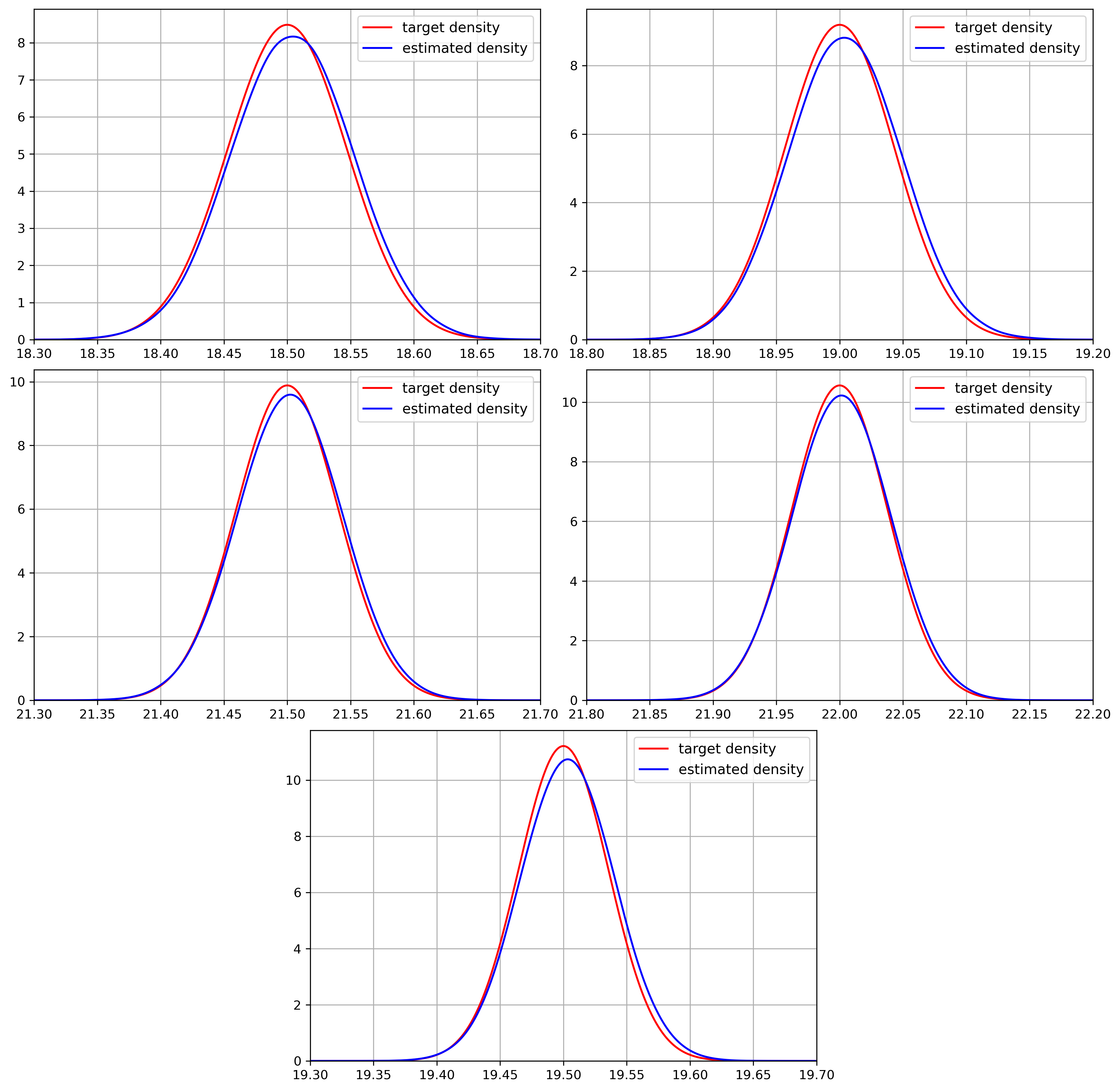
Figure 2: Comparison of the estimated marginal densities of $X_{T}$ with their respective target densities in dimension $d=5$ with $K=100$.

Appendices

Appendix A Relative entropy related results

A.1 Girsanov theorem under finite entropy condition

The first theorem of this Appendix is a well-known result, which can be established for instance by combining the proofs of Theorems 2.1,2.3, 2.6 and 2.9 in [36].

Theorem A.1.

Let $b:[0,T]\times\Omega\rightarrow{\mathbb{R}}^{d}$ and $a:[0,T]\times\Omega\rightarrow S_{d}^{+}$ be two progressively measurable processes. Let ${\mathbb{P}}\in{\cal P}(\Omega)$ such that under ${\mathbb{P}}$ the canonical process has decomposition

$$X_{t}=X_{0}+\int_{0}^{t}b_{r}dr+M_{t}^{\mathbb{P}}+(q{\mathds{1}}_{\{|q|>1\}})*\mu^{X}_{t}+(q{\mathds{1}}_{\{|q|\leq 1\}})*(\mu^{X}-\mu^{L})_{t},$$ (A.1)

where $M^{\mathbb{P}}$ is a continuous local martingale such that $[M^{\mathbb{P}}]=\int_{0}^{\cdot}a_{r}dr$ and $\mu^{L}(X,dt,dq)=L(t,X,dq)dt$ for some Lévy kernel $L$, see Definition 2.2.

Let $\mathbb{Q}\in{\cal P}(\Omega)$ such that $H(\mathbb{Q}|{\mathbb{P}})<+\infty$. Then, there exists a progressively measurable process $\alpha$ and a $\tilde{\cal P}$-measurable function $Y$ such that the following holds.

• Under $\mathbb{Q}$ the canonical process decomposes as

  $$X_{t} =X_{0}+\int_{0}^{t}b_{r}dr+\int_{0}^{t}a_{r}\alpha_{r}dr+(q{\mathds{1}}_{\{|q|\leq 1\}}(Y-1))*\mu^{L}_{t}+M_{t}^{\mathbb{Q}}$$ (A.2)

  $$+(q{\mathds{1}}_{\{|q|>1\}})*\mu^{X}_{t}+(q{\mathds{1}}_{\{|q|\leq 1\}})*(\mu^{X}-(Y.\mu^{L}))_{t},$$

  where $M^{\mathbb{Q}}$ is a continuous $\mathbb{Q}$-local martingale such that $[M^{\mathbb{Q}}]=\int_{0}^{\cdot}a_{r}dr$ and the $\mathbb{Q}$-compensator $Y.\mu^{L}$ of $\mu^{X}$ is given by $(Y.\mu^{L})(X,dt,dq)=Y(X,t,q)\mu^{L}(X,dt,dq)$.

• $$H(\mathbb{Q}|{\mathbb{P}})\geq H(\mathbb{Q}_{0}|{\mathbb{P}}_{0})+\frac{1}{2}{\mathbb{E}}^{\mathbb{Q}}\left[\int_{0}^{T}\alpha_{r}^{\top}a_{r}\alpha_{r}dr\right]+{\mathbb{E}}^{\mathbb{Q}}\left[(Y\log(Y)-Y+1)*\mu^{L}_{T}\right],$$ (A.3)

  and equality holds in (A.3) if the martingale problem, in the sense Remark 3.3, verified by ${\mathbb{P}}$ has a unique solution.

Remark A.2.

Let us take into account the notion of characteristics of a semimartingale, see e.g. Definition 2.6, Chapter II in [32], with truncation function $k(x)=1_{\{|x|\leq 1\}}.$

By Remark 2.8, Theorem A.1 implies in particular that the new characteristics $(B^{\mathbb{Q}},C^{\mathbb{Q}},\mu^{\mathbb{Q}})$ of $X$ related to $\mathbb{Q}$ are

$$\left\{\begin{aligned} &B^{\mathbb{Q}}_{t}=b_{t}+a_{r}\alpha_{t}+(q{\mathds{1}}_{\{|q|\leq 1\}}(Y-1))*\mu^{L}_{t}\\ &C^{\mathbb{Q}}_{t}=a_{t}\\ &\mu^{\mathbb{Q}}=Y\mu^{L}.\end{aligned}\right.$$

A.2 Relative entropy between laws of càdlàg semimartingales

In this section we aim at computing the relative entropy between the laws of two càdlàg semi-martingales, when it exists. In this framework we do not assume a priori the finiteness of the entropy between the two probabilities. The result below is a generalization of Lemma 4.4 in [35], where the considered semimartingales were continuous. Let $L$ be a Lévy kernel in the sense of Definition 2.2 and set $\mu^{L}:=L(t,X,dq)dt$. Let $b^{1},b^{2}:[0,T]\times\Omega\rightarrow{\mathbb{R}}^{d}$, and $a:[0,T]\times\Omega\rightarrow S_{d}^{++}$ be progressively measurable processes. Let $\lambda^{1},\lambda^{2}:\Omega\times[0,T]\times{\mathbb{R}}^{d}\rightarrow{\mathbb{R}}^{+}_{*}$ be two non-negative $\tilde{\cal P}$-measurable functions. Let ${\mathbb{P}}^{1},{\mathbb{P}}^{2}\in{\cal P}(\Omega)$ such that for $i=1,2$, the canonical process decomposes under ${\mathbb{P}}^{i}$

$$X_{t}=X_{0}+\int_{0}^{t}b^{i}_{r}(r,X)dr+M^{{\mathbb{P}}^{i}}_{t}+(q{\mathds{1}}_{\{|q|>1\}})*\mu^{X}+(q{\mathds{1}}_{\{|q|\leq 1\}})*(\mu^{X}-\mu^{i})_{t},$$ (A.4)

where

1. $M^{{\mathbb{P}}^{i}}$ is a continuous ${\mathbb{P}}^{i}$-local martingale verifying $[M^{{\mathbb{P}}^{i}}]=\int_{0}^{\cdot}a(r,X)dr$;

2. $\mu^{i}(X,dt,dq):=\lambda^{i}(X,t,q)L(t,X,dq)dt$.

From now on we use the notation $b_{r}:=b(r,X),\ a_{r}:=a(r,X),r\in[0,T].$

Below we will need the following assumptions for $(b^{1},a,\lambda^{1}L)$ and on the probability ${\mathbb{P}}^{1}$. We set $\eta_{0}={\mathbb{P}}^{1}_{0}$.

Hypothesis A.3.

(Uniqueness and flow existence).

• ${\mathbb{P}}^{1}$ is the unique probability under which decomposition (A.4) holds with $X_{0}\sim\eta_{0}$.

• The triplet $(b^{1},a,\lambda^{1}L)$ verifies the flow existence property with associated progressively measurable kernel $({\mathbb{P}}^{s,\omega})_{(s,\omega)\in[0,T]\times\Omega}$ in the sense of Definition 2.9.

The assumption below concerns both probabilities ${\mathbb{P}}^{1},{\mathbb{P}}^{2}$ and the triplets $(b^{1},a,\lambda^{1}L)$ and $(b^{2},a,\lambda^{2}L)$.

Hypothesis A.4.

(Almost surely finite). We suppose

$$\int_{0}^{T}(b^{1}_{r}-b^{2}_{r})^{\top}a_{r}^{-1}(b^{1}_{r}-b^{2}_{r})dr<+\infty\quad{\mathbb{P}}^{2}\text{-a.s.}$$ (A.5)

and

$$\int_{[0,T]\times{\mathbb{R}}^{d}}|q|{\mathds{1}}_{\{|q|\leq 1\}}|\lambda^{2}-\lambda^{1}|L(r,X,dq)dr<+\infty\quad{\mathbb{P}}^{2}\text{-a.s.}$$ (A.6)

Under Hypothesis A.4 we also introduce the following notations.

$$Y:=\frac{\lambda^{1}}{\lambda^{2}},\quad\alpha:=a^{-1}\left(b^{1}-b^{2}-\int_{{\mathbb{R}}^{d}}q{\mathds{1}}_{\{|q|\leq 1\}}(\lambda^{1}-\lambda^{2})L(\cdot,\cdot,dq)\right),\quad M:=\int_{0}^{\cdot}\alpha_{r}^{\top}dM_{r}^{{\mathbb{P}}^{2}}.$$ (A.7)

Proposition A.5.

Let $a,b^{i},\lambda^{i},{\mathbb{P}}^{i}$, $i=1,2$ be as above. Assume Hypotheses A.3, A.4 and

$${\mathbb{E}}^{{\mathbb{P}}^{2}}\left[\frac{1}{2}\int_{0}^{T}\alpha_{r}^{\top}a_{r}\alpha_{r}dr+\left(\frac{\lambda^{2}}{\lambda^{1}}\log\left(\frac{\lambda^{2}}{\lambda^{1}}\right)-\frac{\lambda^{2}}{\lambda^{1}}+1\right)*\mu^{1}_{T}\right]<+\infty.$$ (A.8)

Suppose ${\mathbb{P}}^{2}_{0}\sim\eta_{0}$. Then $H({\mathbb{P}}^{2}|{\mathbb{P}}^{1})<+\infty$ and

$$H({\mathbb{P}}^{2}|{\mathbb{P}}^{1})=H({\mathbb{P}}^{2}_{0}|{\mathbb{P}}^{1}_{0})+{\mathbb{E}}^{{\mathbb{P}}^{2}}\left[\frac{1}{2}\int_{0}^{T}\alpha_{r}^{\top}a_{r}\alpha_{r}dr+\left(\frac{\lambda^{2}}{\lambda^{1}}\log\left(\frac{\lambda^{2}}{\lambda^{1}}\right)-\frac{\lambda^{2}}{\lambda^{1}}+1\right)*\mu^{1}_{T}\right]<+\infty.$$ (A.9)

The proof of Proposition A.5 requires some intermediate results. For simplicity we suppose $\eta_{0}=\delta_{x}$ for some $x\in{\mathbb{R}}^{d}$ so that $H({\mathbb{P}}^{2}_{0}|{\mathbb{P}}^{1}_{0})=0$, see Remark A.9 below. Notice first that (A.8) implies that

$${\mathbb{E}}^{{\mathbb{P}}^{2}}\left[\left(\frac{\lambda^{2}}{\lambda^{1}}\log\left(\frac{\lambda^{2}}{\lambda^{1}}\right)-\frac{\lambda^{2}}{\lambda^{1}}+1\right)*\mu^{1}_{T}\right] ={\mathbb{E}}^{{\mathbb{P}}^{2}}\left[\left(\lambda^{2}\log\left(\frac{\lambda^{2}}{\lambda^{1}}\right)-\lambda^{2}+\lambda^{1}\right)*\mu^{L}_{T}\right]$$

$$={\mathbb{E}}^{{\mathbb{P}}^{2}}\left[\left(\frac{\lambda^{1}}{\lambda^{2}}-\log\left(\frac{\lambda^{1}}{\lambda^{2}}\right)-1\right)*\mu^{2}_{T}\right]$$

$$={\mathbb{E}}^{{\mathbb{P}}^{2}}\left[\left(Y-\log(Y)-1\right)*\mu^{2}_{T}\right]<+\infty,$$

the latter expectation being well-defined since $x\in]0,+\infty[\mapsto x-\log(x)-1\geq 0$. Hence the triplet $(Y,{\mathbb{P}}^{2},\lambda^{2}L)$ verifies Hypothesis D.1 below and by Lemma D.2 $M+(Y-1)*(\mu^{X}-\mu^{2})$ is a well-defined ${\mathbb{P}}^{2}$-local martingale and the Doléans-Dade exponential $Z:={\cal E}\left(M+(Y-1)*(\mu^{X}-\mu^{2})\right)$ is well-defined (see e.g. Theorem 4.61, Chapter I in [32]), and by Lemma D.3 rewrites

$$Z=\exp\left(M+\log(Y)*(\mu^{X}-\mu^{2})-\frac{1}{2}[M]-\left(Y-\log(Y)-1\right)*\mu^{2}\right).$$ (A.10)

The local martingale $Z$ will constitute the basis for the proof of Proposition A.5. Let then $(\tau_{k})_{k\geq 0}$ be a localizing sequence for $Z$ as well as $M$ and $\log(Y)*(\mu^{X}-\mu^{2})$ appearing in (A.10). For any $k\geq 0$, we also define the probability measure $\mathbb{Q}^{k}$ by

$$d\mathbb{Q}^{k}:=Z^{\tau_{k}}_{T}d{\mathbb{P}}^{2},$$ (A.11)

where $Z^{\tau_{k}}:=Z_{\cdot\wedge\tau_{k}}$.

Remark A.6.

Recall that, since $Z_{t}^{\tau_{k}}={\mathbb{E}}^{{\mathbb{P}}^{2}}[Z_{T}^{\tau_{k}}|{\cal F}_{t}]$ for all $t\in[0,T]$, the martingale $Z^{\tau_{k}}$ is uniformly integrable. Indeed any martingale defined on a compact interval is uniformly integrable. This property easily follows from De la Vallée Poussin criteria of uniform integrability applied to the family $\{{\mathbb{E}}^{\mathbb{P}}[Z_{T}|{\cal F}_{t}]~:~t\in[0,T]\}$, see e.g. T22, Chapter II in [39] for a statement and a proof of this criteria.

Lemma A.7 below constitutes a crucial step for the proof of Proposition A.5. Using Girsanov’s theorem, we express the characteristics of the canonical process $X$ under $\mathbb{Q}_{k}$. Then, relying on decomposition (A.4) as well as Hypothesis A.3, we prove the following.

Lemma A.7.

We formulate the same assumptions as in Proposition A.5. Let $\mathbb{Q}^{k}\in{\cal P}(\Omega)$ be defined in (A.11). Then the restriction of $\mathbb{Q}^{k}$ to $\sigma$-field ${\cal F}_{\tau_{k}}$ equals $({\mathbb{P}}^{1})^{\tau_{k}}$.

Proof.

We keep in mind the notation (A.7). Since $Z^{\tau_{k}}$ is a uniformly integrable ${\mathbb{P}}^{2}$-martingale (see Remark A.6), Theorem 15.3.10 and Remark 15.3.11 in [14] applied with $\mathbb{Q}=\mathbb{Q}_{k}$, ${\mathbb{P}}={\mathbb{P}}^{2}$, $f=\alpha{\mathds{1}}_{\llbracket 0,\tau_{k}\rrbracket}$, $\alpha_{p}=\left(Y{\mathds{1}}_{\llbracket 0,\tau_{k}\rrbracket}\right)\mu^{2}$, $A=Y{\mathds{1}}_{\llbracket 0,\tau_{k}\rrbracket}$, $\mu_{p}^{X}=\mu^{2}{\mathds{1}}_{\llbracket 0,\tau_{k}\rrbracket}$, states that under $\mathbb{Q}^{k}$ the canonical process $X$ has decomposes as

$$\begin{aligned} X_{t}&=x+\int_{0}^{t}\left({\mathds{1}}_{\llbracket 0,\tau_{k}\rrbracket}b^{2}\right)(r,X)dr+\bar{M}_{t}+\int_{0}^{t}({\mathds{1}}_{\llbracket 0,\tau_{k}\rrbracket}a\alpha)(r,X)dr+\left(q{\mathds{1}}_{\{|q|\leq 1\}}(Y-1)\right)*\left({\mathds{1}}_{\llbracket 0,\tau_{k}\rrbracket}\mu^{2}\right)_{t}\\ &+\left(q{\mathds{1}}_{\{|q|>1\}}\right)*\mu^{X}_{t}+\left(q{\mathds{1}}_{\{|q|\leq 1\}}\right)*(\mu^{X}-\left(Y{\mathds{1}}_{\llbracket 0,\tau_{k}\rrbracket}\mu^{2})\right)_{t},\end{aligned}$$ (A.12)

where $\bar{M}$ is a continuous local martingale under $\mathbb{Q}^{k}$ with $[\bar{M}]=\int_{0}^{\cdot}{\mathds{1}}_{\llbracket 0,\tau_{k}\rrbracket}a_{r}dr.$ Stopping the process $X$ in (A.12) at $\tau_{k}$, we get the following decomposition for the stopped canonical process $X_{\cdot\wedge\tau_{k}}$,

$$X_{t\wedge\tau_{k}} =x+\int_{0}^{t\wedge\tau_{k}}b^{2}(r,X)dr+\bar{M}_{t\wedge\tau_{k}}+\int_{0}^{t\wedge\tau_{k}}(a\alpha)(r,X)dr+\left(q{\mathds{1}}_{\{|q|\leq 1\}}(Y-1)\right)*\mu^{2}_{t\wedge\tau_{k}}$$ (A.13)

$$+\left(q{\mathds{1}}_{\{|q|>1\}}\right)*\mu^{X}_{t\wedge\tau_{k}}+\left(q{\mathds{1}}_{\{|q|\leq 1\}}\right)*(\mu^{X}-(Y.\mu^{2}))_{t\wedge\tau_{k}}.$$

Using the expression (A.7) of $Y$ and $\alpha$, we have that

$$\int_{0}^{t\wedge\tau_{k}}(a\alpha)(r,X)dr =\int_{0}^{t\wedge\tau_{k}}b^{1}(r,X)dr-\int_{0}^{t\wedge\tau_{k}}b^{2}(r,X)dr$$ (A.14)

$$-\int_{[0,t\wedge\tau_{k}]\times{\mathbb{R}}^{d}}q{\mathds{1}}_{\{|q|\leq 1\}}(\lambda^{1}-\lambda^{2})L(r,X,dq)dr,$$

$$\left(q{\mathds{1}}_{\{|q|\leq 1\}}(Y-1)\right)*\mu^{2}_{t\wedge\tau_{k}}=\int_{[0,t\wedge\tau_{k}]\times{\mathbb{R}}^{d}}q{\mathds{1}}_{\{|q|\leq 1\}}(\lambda^{1}-\lambda^{2})L(r,X,dq)dr,$$ (A.15)

and

$$\left(q{\mathds{1}}_{\{|q|\leq 1\}}\right)*(\mu^{X}-(Y.\mu^{2}))_{t\wedge\tau_{k}}=(q{\mathds{1}}_{\{|q|\leq 1\}})*(\mu^{X}-\mu^{1})_{t\wedge\tau_{k}}.$$ (A.16)

Injecting (A.14), (A.15) and (A.16) in (A.13) yields the decomposition

$$X_{t\wedge\tau_{k}}=x+\int_{0}^{t\wedge\tau_{k}}b^{1}(r,X)dr+\bar{M}_{t\wedge\tau_{k}}+(q{\mathds{1}}_{\{|q|>1\}})*\mu^{X}_{t\wedge\tau_{k}}+(q{\mathds{1}}_{\{|q|\leq 1\}})*(\mu^{X}-\mu^{1})_{t\wedge\tau_{k}}.$$ (A.17)

It follows from (A.17) that, under $\mathbb{Q}^{k}$, the canonical process has decomposition (A.4) with $i=1$ stopped at $\tau_{k}$. However it is not immediate that the uniqueness of the decomposition (A.4) with $i=1$ given by Hypothesis A.3 carries over to the random interval $[0,\tau_{k}]$. This is the object of the rest of the proof.

Let $({\mathbb{P}}^{s,\omega})_{(s,\omega)\in[0,T]\times\Omega}$ the the the path-dependent class provided by Hypothesis A.3. We set $\omega\in\Omega\mapsto\mathbb{Q}_{\omega}:={\mathbb{P}}^{\tau_{k}(\omega),\omega_{\cdot\wedge\tau_{k}(\omega)}}$. The mapping $\omega\mapsto\mathbb{Q}_{\omega}$ satisfies the following properties.

1. We can show that, $A\in{\cal F}$, the map $\omega\mapsto\mathbb{Q}_{\omega}(A)$ is ${\cal F}_{\tau_{k}}$-measurable for any $A\in{\cal F}$. To see this, we introduce the map $\Psi:\omega\mapsto(\tau_{k}(\omega),\omega_{\cdot\wedge\tau_{k}(\omega)})$ which is $({\cal F}_{\tau_{k}},{\cal B}([0,T])\otimes{\cal F})$-measurable. Indeed, $\omega\mapsto\tau_{k}(\omega)$ is obviously ${\cal F}_{\tau_{k}}$-measurable, and since $\tau_{k}$ is a stopping time and $\omega\in\Omega\mapsto\omega$ is càdlàg, $\omega\mapsto\omega_{\cdot\wedge\tau_{k}(\omega)}$ is also ${\cal F}_{\tau_{k}}$-measurable, and the measurability of $\Psi$ follows. Denoting $\Phi:(s,\omega)\mapsto{\mathbb{P}}^{s,\omega}(A)$, the map $\omega\mapsto\mathbb{Q}_{\omega}(A)$ can be written as the composition $\Phi\circ\Psi$. Since $\Psi$ is ${\cal F}_{\tau_{k}}$-measurable, and since $\Phi$ is measurable by definition, $\Phi\circ\Psi$ is ${\cal F}_{\tau_{k}}$ measurable.

2. $\mathbb{Q}_{\omega}\left(X_{\tau_{k}(\omega)}=X_{\tau_{k}(\omega)}(\omega)\right)={\mathbb{P}}^{\tau_{k}(\omega),\omega_{\cdot\wedge\tau_{k}(\omega)}}\left(X_{r}=\omega_{r},0\leq r\leq\tau_{k}(\omega)\right)=1$ for all $\omega\in\Omega$.

Then by Theorem 6.1.2 in [46] there exists a unique probability measure $\mathbb{Q}\in{\cal P}(\Omega)$ such that $\mathbb{Q}=\mathbb{Q}^{k}$ on ${\cal F}_{\tau_{k}}$ and $(\mathbb{Q}_{\omega})_{\omega\in\Omega}$ is a regular conditional probability distribution of $\mathbb{Q}$ given ${\cal F}_{\tau_{k}}$, see the definition just before Theorem 1.1.6 in [46]. We are going to prove that, under $\mathbb{Q}$, the canonical process has decomposition (A.4) with $i=1$. To this aim, we take into account Remark 2.8. Let $h$ be a bounded ${\cal C}^{2}$-function. We define

$$N[h] :=h(X_{\cdot})-h(x)-\int_{0}^{\cdot}{\cal L}^{1}(h)(r,X)dr,$$

where

$${\cal L}^{1}(h)(t,X) :=\langle\nabla_{x}h(t,X_{t}),b^{1}(t,X)\rangle+\frac{1}{2}Tr[a(t,X)\nabla_{x}^{2}h(t,X_{t})]$$

$$+\int_{{\mathbb{R}}^{d}}\left(h(t,X_{t-}+q)-h(t,X_{t-})-\langle\nabla_{x}h(X_{t-}),q\rangle{\mathds{1}}_{\{|q|\leq 1\}}\right)\mu^{1}(t,X,dq).$$

We need to prove that $N[h]$ is a local martingale under $\mathbb{Q}$. We fix $n\in{\mathbb{N}}^{*}$. We also introduce the sequence of stopping times

$$\sigma_{n}:=\inf\left\{t\in[0,T]~:~\int_{0}^{t}{\cal L}^{1}(h)(r,X)dr\geq n\right\},~n\geq 1.$$

We prove below that $N[h]^{\sigma_{n}}$ is a $\mathbb{Q}$-martingale.

We have the following two facts.

1. By decomposition (A.17) and Itô’s formula, the process $N[h]_{\cdot\wedge\tau_{k}}$ is a local martingale under $\mathbb{Q}^{k}$. Since $N[h]^{\sigma_{n}}_{\cdot\wedge\tau_{k}}$ is bounded, it is a martingale under $\mathbb{Q}_{k}$.

2. We recall Hypothesis A.3 which states that $(P^{s,\omega})$ verifies the flow existence property, see Definition 2.9, with respect to $(b^{1},a,\lambda^{1}L)$. We recall that $\mathbb{Q}_{\omega}={\mathbb{P}}^{\tau_{k}(\omega),\omega_{\cdot\wedge\tau_{k}(\omega)}}$. By decomposition (2.4) applied with $b=b^{1}$, $L=\lambda^{1}L$ and $s=\tau_{k}(\omega)$, together with Itô’s formula, the process $N[h]_{\cdot\wedge\tau_{k}}-N[h]_{\cdot\wedge\tau_{k}(\omega)}$ is a local martingale under $\mathbb{Q}_{\omega}$. Consequently the stopped process $N[h]^{\sigma_{n}}_{\cdot\wedge\tau_{k}}-N[h]^{\sigma_{n}}_{\cdot\wedge\tau_{k}(\omega)}$ is a local $\mathbb{Q}_{\omega}$-martingale, therefore a genuine martingale since it is bounded.

Using the final conclusion of Theorem 6.1.2 in [46], see Remark A.8 below, it follows from previous items 1. and 2. that the process $N[h]^{\sigma_{n}}$ is a martingale under $\mathbb{Q}$. Finally $N[h]$ is indeed a local martingale under $\mathbb{Q}$, hence indeed, that under $\mathbb{Q}$ the canonical process has decomposition (A.4) with $i=1$.

By the uniqueness item of such decomposition, see Hypothesis A.3, we get $\mathbb{Q}={\mathbb{P}}^{1}$. This implies in particular that $\mathbb{Q}^{\tau_{k}}=({\mathbb{P}}^{1})^{\tau_{k}}$. By construction, we have $\mathbb{Q}=\mathbb{Q}^{k}$ on ${\cal F}_{\tau_{k}}$, hence $\mathbb{Q}^{\tau_{k}}=(\mathbb{Q}^{k})^{\tau_{k}}$ yielding by what precedes that $(\mathbb{Q}^{k})^{\tau_{k}}=({\mathbb{P}}^{1})^{\tau_{k}}$. This concludes the proof.

∎

Remark A.8.

Theorem 6.1.2 in [46] applies to the case where $\Omega=C([0,T],{\mathbb{R}}^{d})$, but its proof remains valid without any modification when $\Omega=D([0,T],{\mathbb{R}}^{d})$.

We are now ready to prove Proposition A.5.

Proof of Proposition A.5..

Recall the definition (A.11) of the probability measure $\mathbb{Q}^{k}$. By Lemma A.7, we have $(\mathbb{Q}^{k})^{\tau_{k}}=({\mathbb{P}}^{1})^{\tau_{k}}$. Then $d({\mathbb{P}}^{1})^{\tau_{k}}=Z_{T}^{\tau_{k}}d({\mathbb{P}}^{2})^{\tau_{k}}$ and since $Z_{T}^{\tau_{k}}>0$, $({\mathbb{P}}^{2})^{\tau_{k}}\ll({\mathbb{P}}^{1})^{\tau_{k}}$ and $d({\mathbb{P}}^{2})^{\tau_{k}}=\left(1/Z^{\tau_{k}}_{T}\right)d({\mathbb{P}}^{1})^{\tau_{k}}$. We focus now on the process $1/Z^{\tau_{k}}$, which rewrites by (A.10)

$$\frac{1}{Z^{\tau_{k}}}=\exp\left(-N_{\cdot\wedge\tau_{k}}+\frac{1}{2}[M]_{\cdot\wedge\tau_{k}}+\left((Y-\log(Y)-1)\right)*\mu^{2}_{\cdot\wedge\tau_{k}}\right),$$

where $N:=M+\log(Y)*(\mu^{X}-\mu^{2})$ is a ${\mathbb{P}}^{2}$-local martingale. $N_{\cdot\wedge\tau_{k}}$ is a true ${\mathbb{P}}^{2}$-martingale, and we then have

$$H(({\mathbb{P}}^{2})^{\tau_{k}}|({\mathbb{P}}^{1})^{\tau_{k}}) =-{\mathbb{E}}^{({\mathbb{P}}^{2})^{\tau_{k}}}\left[\log Z^{\tau_{k}}_{T}\right]$$

$$={\mathbb{E}}^{({\mathbb{P}}^{2})^{\tau_{k}}}\left[\frac{1}{2}\int_{0}^{T\wedge\tau_{k}}\alpha_{r}^{\top}a_{r}\alpha_{r}dr+\left((Y-\log(Y)-1)\right)*\mu^{2}_{T\wedge\tau_{k}}\right]$$

$$={\mathbb{E}}^{{\mathbb{P}}^{2}}\left[\frac{1}{2}\int_{0}^{T\wedge\tau_{k}}\alpha_{r}^{\top}a_{r}\alpha_{r}dr+\left((Y-\log(Y)-1){\mathds{1}}_{\llbracket 0,\tau_{k}\rrbracket}\right)*\mu^{2}_{T\wedge\tau_{k}}\right]$$

$$\leq{\mathbb{E}}^{{\mathbb{P}}^{2}}\left[\frac{1}{2}\int_{0}^{T}\alpha_{r}^{\top}a_{r}\alpha_{r}dr+\left(Y-\log(Y)-1\right)*\mu^{2}_{T}\right]$$

$$={\mathbb{E}}^{{\mathbb{P}}^{2}}\left[\frac{1}{2}\int_{0}^{T}\alpha_{r}^{\top}a_{r}\alpha_{r}dr+\left(\frac{\lambda^{2}}{\lambda^{1}}\log\left(\frac{\lambda^{2}}{\lambda^{1}}\right)-\frac{\lambda^{2}}{\lambda^{1}}+1\right)*\mu^{1}_{T}\right],$$

recalling that $\mu^{i}=\lambda^{i}\mu^{L},i=1,2.$ Now since $({\mathbb{P}}^{1})^{\tau_{k}}\underset{k\rightarrow+\infty}{\longrightarrow}{\mathbb{P}}^{1}$ and $({\mathbb{P}}^{2})^{\tau_{k}}\underset{k\rightarrow+\infty}{\longrightarrow}{\mathbb{P}}^{2}$ weakly, the joint lower semi-continuity of the relative entropy for the weak* convergence on Polish spaces (see Remark 2.4 item 2.) yields

$$H({\mathbb{P}}^{2}|{\mathbb{P}}^{1})\leq{\mathbb{E}}^{{\mathbb{P}}^{2}}\left[\frac{1}{2}\int_{0}^{T}\alpha_{r}^{\top}a_{r}\alpha_{r}dr+\left(\frac{\lambda^{2}}{\lambda^{1}}\log\left(\frac{\lambda^{2}}{\lambda^{1}}\right)-\frac{\lambda^{2}}{\lambda^{1}}+1\right)*\mu^{1}_{T}\right].$$ (A.18)

The inequality (A.18) implies by (A.8) that $H({\mathbb{P}}^{2}|{\mathbb{P}}^{1})<+\infty$. Theorem A.1 then applies and we directly deduce from (A.3) that

$$H({\mathbb{P}}^{2}|{\mathbb{P}}^{1})\geq{\mathbb{E}}^{{\mathbb{P}}^{2}}\left[\frac{1}{2}\int_{0}^{T}\alpha_{r}^{\top}a_{r}\alpha_{r}dr+\left(\frac{\lambda^{2}}{\lambda^{1}}\log\left(\frac{\lambda^{2}}{\lambda^{1}}\right)-\frac{\lambda^{2}}{\lambda^{1}}+1\right)*\mu^{1}_{T}\right].$$

This concludes the proof. ∎

Remark A.9.

In the more general setting where we only assume that ${\mathbb{P}}^{2}_{0}\sim\eta_{0}$, we simply replace the density $Z$ in (A.10) by $\tilde{Z}:=(d{\mathbb{P}}^{1}_{0}/d{\mathbb{P}}^{2}_{0})Z$ and the proof follows exactly the same line as in the case $\eta_{0}=\delta_{x}$.

In the corollary below we remove the assumption ${\mathbb{P}}^{2}_{0}\sim\eta_{0}$. This will raise some technical difficulties.

Corollary A.10.

Assume that, under ${\mathbb{P}}^{i}$, $i=1,2$, the canonical process has decomposition (A.4).

Assume Hypotheses A.3 (which only concerns ${\mathbb{P}}^{1}$) and A.4. Assume moreover that (A.8) holds. Then

$$H({\mathbb{P}}^{2}|{\mathbb{P}}^{1})=H({\mathbb{P}}^{2}_{0}|{\mathbb{P}}^{1}_{0})+{\mathbb{E}}^{{\mathbb{P}}^{2}}\left[\frac{1}{2}\int_{0}^{T}\alpha_{r}^{\top}a_{r}\alpha_{r}dr+\left(\frac{\lambda^{2}}{\lambda^{1}}\log\left(\frac{\lambda^{2}}{\lambda^{1}}\right)-\frac{\lambda^{2}}{\lambda^{1}}+1\right)*\mu^{1}_{T}\right].$$

which raises some technical difficulties: in particular the r.v. $\tilde{Z}$ in Remark A.9 is not properly defined.

Indeed, the proof of that Corollary is based on Lemma A.11 below, which states a disintegration result. The proof of that lemma can be found in [8] and it is based on the equivalence criterion in Remark 2.8. Similar arguments are developed in the uniqueness part of Theorem 4.5 in [28].

Lemma A.11.

Let ${\mathbb{P}}\in{\cal P}(\Omega)$ such that, under ${\mathbb{P}}$, the canonical process has decomposition (A.1) with initial law $\eta_{0}$.

1. There is a measurable kernel $({\mathbb{P}}(x))_{x\in{\mathbb{R}}^{d}}$ such that ${\mathbb{P}}=\int_{{\mathbb{R}}^{d}}{\mathbb{P}}(x)\eta_{0}(dx)$, where for $\eta_{0}$-almost all $x\in{\mathbb{R}}^{d}$, under ${\mathbb{P}}(x)$, the canonical process decomposes as

   $$X_{t}=x+\int_{0}^{t}b_{r}dr+M^{0,x}_{t}+\left(q{\mathds{1}}_{\{|q|>1\}}\right)*\mu^{X}_{t}+\left(q{\mathds{1}}_{\{|q|\leq 1\}}\right)*(\mu^{X}-\mu^{L})_{t},$$ (A.19)

   where $M^{0,x}$ is a continuous ${\mathbb{P}}(x)$-local martingale verifying $[M^{0,x}]=\int_{0}^{\cdot}a_{r}dr$.

2. Assume moreover that, given $b$ and $\eta_{0}$, the decomposition (A.19) is unique in law. Then the decomposition (A.19) is also unique in law for $\eta_{0}$-almost all $x\in{\mathbb{R}}^{d}$.

Proof of Corollary A.10..

The result is trivial if $H({\mathbb{P}}^{2}_{0}|{\mathbb{P}}^{1}_{0})=+\infty$, so we can suppose $H({\mathbb{P}}^{2}_{0}|{\mathbb{P}}^{1}_{0})<+\infty$. We set $\eta_{0}^{1}:={\cal L}^{{\mathbb{P}}^{1}}(X_{0})$ and $\eta_{0}^{2}:={\cal L}^{{\mathbb{P}}^{2}}(X_{0})$. We have the following.

1. Let $i=1,2$. Lemma A.11 item 1. applied with ${\mathbb{P}}={\mathbb{P}}^{i}$ provides the existence of a measurable kernel $({\mathbb{P}}^{i}(x))_{x\in{\mathbb{R}}^{d}}$ and an $\eta_{0}^{1}$-null set ${\cal N}_{1}$ such that ${\mathbb{P}}^{i}=\int_{{\mathbb{R}}^{d}}{\mathbb{P}}^{i}(x)\eta_{0}^{i}(dx)$ and for all $x\in{\cal N}_{i}^{c}$, the canonical process $X$ has decomposition (A.19) with $b=b^{i}$ and $\mu^{L}=\mu^{i}$ under ${\mathbb{P}}^{i}(x)$.

2. Moreover, since decomposition (A.4) (given $\eta^{1}_{0},b^{1}$ and $\mu^{1}$), is unique in law, item 2. of the same lemma states that one can chose ${\cal N}_{1}$ such that for all $x\in{\cal N}_{1}^{c}$, decomposition (A.19) under ${\mathbb{P}}^{1}(x)$ is unique in law.

Recall that $H(\eta_{0}^{2}|\eta_{0}^{1})=H({\mathbb{P}}_{0}^{2}|{\mathbb{P}}_{0}^{1})<+\infty$. This implies in particular that $\eta_{0}^{2}\ll\eta_{0}^{1}$, hence ${\cal N}_{1}$ is also an $\eta_{0}^{2}$-null set and ${\cal N}:={\cal N}_{1}\cup{\cal N}_{2}$ is an $\eta_{0}^{2}$-null set. On the one hand, by Lemma 2.3 in [21],

$$H({\mathbb{P}}^{2}|{\mathbb{P}}^{1})=H(\eta_{0}^{2}|\eta_{0}^{1})+\int_{{\mathbb{R}}^{d}}H({\mathbb{P}}(x)^{2}|{\mathbb{P}}(x)^{1})\eta_{0}^{2}(dx).$$ (A.20)

On the other hand, for all $x\in{\cal N}^{c}$, a direct application of Proposition A.5 with ${\mathbb{P}}^{1}={\mathbb{P}}^{1}(x)$ and ${\mathbb{P}}^{2}={\mathbb{P}}^{2}(x)$ yields

$$H({\mathbb{P}}^{2}(x)|{\mathbb{P}}^{1}(x))={\mathbb{E}}^{{\mathbb{P}}^{2}(x)}\left[\frac{1}{2}\int_{0}^{T}\alpha_{r}^{\top}a_{r}\alpha_{r}dr+\left(\frac{\lambda^{2}}{\lambda^{1}}\log\left(\frac{\lambda^{2}}{\lambda^{1}}\right)-\frac{\lambda^{2}}{\lambda^{1}}+1\right)*\mu^{1}_{T}\right].$$ (A.21)

The result follows replacing $H({\mathbb{P}}^{2}(x)|{\mathbb{P}}^{1}(x))$ in (A.20) by its expression (A.21). ∎

Appendix B Entropy penalized optimization problem with a prescribed terminal law

Proposition B.1.

Let ${\mathbb{P}}\in{\cal P}(\Omega)$ be fixed. Let $\eta_{T}\in{\cal P}({\mathbb{R}}^{d})$ be a probability measure such that $H(\eta_{T}|{\mathbb{P}}_{T})<+\infty$. Let $\lambda:=d\eta_{T}/d{\mathbb{P}}_{T}$ and $\gamma_{\epsilon}$ be a measurable function such that $\gamma_{\epsilon}(X_{T}):={\mathbb{E}}^{\mathbb{P}}\left[\exp(-\epsilon{\varphi}(X))|X_{T}\right]$, where $\epsilon>0$ and $\varphi:D([0,T],{\mathbb{R}}^{d})\rightarrow{\mathbb{R}}_{+}$ is a bounded Borel function. Set ${\cal P}(\Omega,\eta_{T}):=\{\mathbb{Q}\in{\cal P}(\Omega)~:~\mathbb{Q}_{T}=\eta_{T}\}$. Then

$$\min_{\mathbb{Q}\in{\cal P}(\Omega,\eta_{T})}{\cal J}_{\epsilon}(\mathbb{Q},{\mathbb{P}})=\frac{1}{\epsilon}\int_{{\mathbb{R}}^{d}}\log\frac{\lambda(x)}{\gamma_{\epsilon}(x)}\eta_{T}(dx),\quad\text{where}\quad{\cal J}_{\epsilon}(\mathbb{Q},{\mathbb{P}})={\mathbb{E}}^{\mathbb{Q}}\left[{\varphi}(X)\right]+\frac{1}{\epsilon}H(\mathbb{Q}|{\mathbb{P}}),$$ (B.1)

and there exists a unique minimizer $\mathbb{Q}^{*}\in{\cal P}(\Omega,\eta_{T})$ given by

$$d\mathbb{Q}^{*}:=\exp\left(-\epsilon{\varphi}(X)\right)\frac{\lambda(X_{T})}{\gamma_{\epsilon}(X_{T})}d{\mathbb{P}}.$$ (B.2)

Remark B.2.

$\eta_{T}$ is absolutely continuous with respect to ${\mathbb{P}}_{T}$ so that the Radon-Nikodym density $\lambda$ in the statement makes sense.

Proof.

The proof decomposes into three steps.

1. We first check that $\mathbb{Q}^{*}$ defined by (B.2) is an element of ${\cal P}(\Omega,\eta_{T})$ and

   $${\cal J}_{\epsilon}(\mathbb{Q}^{*},{\mathbb{P}})=\frac{1}{\epsilon}{\mathbb{E}}^{\mathbb{Q}^{*}}\left[\log\frac{\lambda(X_{T})}{\gamma_{\epsilon}(X_{T})}\right]=\frac{1}{\epsilon}\int_{{\mathbb{R}}^{d}}\log\frac{\lambda(x)}{\gamma_{\epsilon}(x)}\eta_{T}(dx).$$ (B.3)

   Moreover ${\cal J}_{\varepsilon}(\mathbb{Q}^{*},{\mathbb{P}})<\infty$.

2. We suppose first $\eta_{T}\sim{\mathbb{P}}_{T}$ and we prove that

   $${\cal J}_{\epsilon}(\mathbb{Q},{\mathbb{P}})\geq\frac{1}{\epsilon}\int_{{\mathbb{R}}^{d}}\log\frac{\lambda(x)}{\gamma_{\epsilon}(x)}\eta_{T}(dx),\quad\forall\mathbb{Q}\in{\cal P}(\Omega,\eta_{T}).$$ (B.4)

3. We establish (B.4) when only $\eta_{T}\ll{\mathbb{P}}_{T}$. In particular, by (B.3), this establishes (B.1).

We proceed proving the previous points.

1. Let us verify that $\mathbb{Q}^{*}\in{\cal P}(\Omega,\eta_{T})$. For $\psi\in{\cal C}_{b}({\mathbb{R}}^{d})$ we have

   $${\mathbb{E}}^{\mathbb{Q}^{*}}[\psi(X_{T})] ={\mathbb{E}}^{{\mathbb{P}}}\left[\psi(X_{T})\exp\left(-\epsilon{\varphi}(X)\right)\frac{\lambda(X_{T})}{\gamma_{\epsilon}(X_{T})}\right]$$

   $$={\mathbb{E}}^{{\mathbb{P}}}\left[\psi(X_{T})\frac{\lambda(X_{T})}{\gamma_{\epsilon}(X_{T})}{\mathbb{E}}^{\mathbb{P}}\left[\exp\left(-\epsilon{\varphi}(X)\right)\middle|X_{T}\right]\right]$$

   $$={\mathbb{E}}^{\mathbb{P}}\left[\psi(X_{T})\frac{\lambda(X_{T})}{\gamma_{\epsilon}(X_{T})}\gamma_{\epsilon}(X_{T})\right]$$

   $$={\mathbb{E}}^{\mathbb{P}}\left[\psi(X_{T})\frac{d\eta_{T}}{d{\mathbb{P}}_{T}}(X_{T})\right]$$

   $$=\int_{{\mathbb{R}}^{d}}\psi(x)\eta_{T}(dx).$$

   Since the previous equality holds for all $\psi\in{\cal C}_{b}({\mathbb{R}}^{d})$, $\mathbb{Q}^{*}_{T}=\eta_{T}$ and $\mathbb{Q}^{*}\in{\cal P}(\Omega,\eta_{T})$.

   We now prove (B.3). By (B.2) we have

   $$\log\frac{d\mathbb{Q}^{*}}{d{\mathbb{P}}}=-\epsilon{\varphi}(X)+\log\frac{\lambda}{\gamma_{\epsilon}}(X_{T})\quad\mathbb{Q}^{*}\text{-a.s.}$$ (B.5)

   since ${\mathbb{P}}$-a.s. Consequently, taking the expectation with respect to $\mathbb{Q}^{*}$ we get

   $$H(\mathbb{Q}^{*}|{\mathbb{P}})=-\epsilon{\mathbb{E}}^{\mathbb{Q}^{*}}{\varphi}(X))+{\mathbb{E}}^{\mathbb{Q}^{*}}\left[\log\frac{\lambda}{\gamma_{\epsilon}}(X_{T})\right].$$ (B.6)

   Since the left-hand side is well-defined by Remark 2.4 item 1. also the second expectation on the right-hand side is well-defined.

   By Definition (B.1) of ${\cal J}_{\epsilon}$ and (B.6) we get

   $${\cal J}_{\epsilon}(\mathbb{Q}^{*},{\mathbb{P}})={\mathbb{E}}^{\mathbb{Q}^{*}}\left[{\varphi}(X)\right]-{\mathbb{E}}^{\mathbb{Q}^{*}}\left[{\varphi}(X)\right]+\frac{1}{\epsilon}{\mathbb{E}}^{\mathbb{Q}^{*}}\left[\log\frac{\lambda(X_{T})}{\gamma_{\epsilon}(X_{T})}\right].$$ (B.7)

   This shows the first equality of (B.3), the second equality follows because $\mathbb{Q}^{*}_{T}=\eta_{T}$.

   Moreover ${\cal J}_{\varepsilon}(\mathbb{Q}^{*},{\mathbb{P}})<\infty$ since

   $${\mathbb{E}}^{\mathbb{Q}^{*}}\left[\log\frac{\lambda}{\gamma_{\epsilon}}(X_{T})\right]=H(\eta_{T}|{\mathbb{P}}_{T})-{\mathbb{E}}^{\eta_{T}}\left[\log(\gamma_{\varepsilon}(X_{T}))\right],$$

   and the expectation on the left-hand side is smaller than $+\infty$, since $\gamma_{\varepsilon}$ is lower bounded by a positive constant ${\mathbb{P}}_{T}$ a.e. therefore $\eta_{T}$ a.e.

2. Assume that $\eta_{T}\sim{\mathbb{P}}_{T}$. This implies in particular that $\mathbb{Q}^{*}\sim{\mathbb{P}}$, taking into account (B.2). Let $\mathbb{Q}\in{\cal P}(\Omega,\eta_{T})$ such that ${\cal J}_{\epsilon}(\mathbb{Q},{\mathbb{P}})<+\infty$, which means equivalently $H(\mathbb{Q}|{\mathbb{P}})<+\infty$. Since $\mathbb{Q}\ll{\mathbb{P}}$ and $\mathbb{Q}^{*}\sim{\mathbb{P}}$, it holds that $\mathbb{Q}\ll\mathbb{Q}^{*}$ and we have

   $$\log\frac{d\mathbb{Q}}{d\mathbb{Q}^{*}} =\log\frac{d\mathbb{Q}}{d{\mathbb{P}}}+\log\frac{d{\mathbb{P}}}{d\mathbb{Q}^{*}}$$

   $$=\log\frac{d\mathbb{Q}}{d{\mathbb{P}}}+\epsilon{\varphi}(X)-\log\frac{\lambda(X_{T})}{\gamma_{\epsilon}(X_{T})},$$

   where the previous equality holds $\mathbb{Q}$-a.s. since it holds ${\mathbb{P}}$-a.s. Taking the expectation under $\mathbb{Q}$ then yields

   $$H(\mathbb{Q}|\mathbb{Q}^{*})=H(\mathbb{Q}|{\mathbb{P}})+\epsilon{\mathbb{E}}^{\mathbb{Q}}[{\varphi}(X)]-{\mathbb{E}}^{\mathbb{Q}}\left[\log\frac{\lambda(X_{T})}{\gamma_{\epsilon}(X_{T})}\right],$$ (B.8)

   and since $\mathbb{Q}_{T}=\eta_{T}$, (B.8) rewrites

   $$H(\mathbb{Q}|\mathbb{Q}^{*})=H(\mathbb{Q}|{\mathbb{P}})+\epsilon{\mathbb{E}}^{\mathbb{Q}}[{\varphi}(X)]-\int_{{\mathbb{R}}^{d}}\log\frac{\lambda(x)}{\gamma_{\epsilon}(x)}\eta_{T}(dx)={\cal J}_{\epsilon}(\mathbb{Q},{\mathbb{P}})-\int_{{\mathbb{R}}^{d}}\log\frac{\lambda(x)}{\gamma_{\epsilon}(x)}\eta_{T}(dx).$$ (B.9)

   Dividing both sides in (B.9) by $\epsilon>0$, we get

   $${\cal J}_{\epsilon}(\mathbb{Q},{\mathbb{P}})=\frac{1}{\epsilon}H(\mathbb{Q}|\mathbb{Q}^{*})+\frac{1}{\epsilon}\int_{{\mathbb{R}}^{d}}\log\frac{\lambda(x)}{\gamma_{\epsilon}(x)}\eta_{T}(dx)\geq\frac{1}{\epsilon}\int_{{\mathbb{R}}^{d}}\log\frac{\lambda(x)}{\gamma_{\epsilon}(x)}\eta_{T}(dx).$$

   This concludes the proof of (B.4).

3. We now turn to the general case. For $\alpha\in]0,1[$, we set $\eta^{\alpha}_{T}:=\alpha{\mathbb{P}}_{T}+(1-\alpha)\eta_{T}$. By convexity of the relative entropy (see Remark 2.4 item 2.), it holds that $H(\eta^{\alpha}_{T}|{\mathbb{P}}_{T})\leq(1-\alpha)H(\eta_{T}|{\mathbb{P}}_{T})<+\infty$. We apply now (B.4) in item 2. replacing ${\cal P}(\Omega,\eta_{T})$ by ${\cal P}(\Omega,\eta^{\alpha}_{T})$. This is possible because $\eta^{\alpha}_{T}\sim{\mathbb{P}}_{T}$, so that

   $${\cal J}_{\epsilon}(\mathbb{Q}^{\alpha},{\mathbb{P}})\geq\frac{1}{\epsilon}\int_{{\mathbb{R}}^{d}}\log\frac{\lambda^{\alpha}(x)}{\gamma_{\epsilon}(x)}\eta^{\alpha}_{T}(dx)=\frac{\alpha}{\epsilon}\int_{{\mathbb{R}}^{d}}\log\frac{\lambda^{\alpha}(x)}{\gamma_{\epsilon}(x)}{\mathbb{P}}_{T}(dx)+\frac{1-\alpha}{\epsilon}\int_{{\mathbb{R}}^{d}}\log\frac{\lambda^{\alpha}(x)}{\gamma_{\epsilon}(x)}\eta_{T}(dx),$$ (B.10)

   where $\lambda^{\alpha}:=d\eta^{\alpha}_{T}/d{\mathbb{P}}_{T}=\alpha+(1-\alpha)\lambda$. On the one hand, for any $\mathbb{Q}\in{\cal P}(\Omega,\eta_{T})$, $\mathbb{Q}^{\alpha}:=\alpha{\mathbb{P}}+(1-\alpha)\mathbb{Q}\in{\cal P}(\Omega,\eta^{\alpha}_{T})$, and again the convexity of the relative entropy yields $H(\mathbb{Q}^{\alpha}|{\mathbb{P}})\leq(1-\alpha)H(\mathbb{Q}|{\mathbb{P}})$. Hence

   $${\cal J}_{\epsilon}(\mathbb{Q}^{\alpha},{\mathbb{P}}) ={\mathbb{E}}^{\mathbb{Q}^{\alpha}}[{\varphi}(X)]+\frac{1}{\epsilon}H(\mathbb{Q}^{\alpha}|{\mathbb{P}})$$ (B.11)

   $$=(1-\alpha){\mathbb{E}}^{\mathbb{Q}}[{\varphi}(X)]+\alpha{\mathbb{E}}^{\mathbb{P}}[{\varphi}(X)]+\frac{1}{\epsilon}H(\mathbb{Q}^{\alpha}|{\mathbb{P}})$$

   $$\leq(1-\alpha){\mathbb{E}}^{\mathbb{Q}}[{\varphi}(X)]+\alpha{\mathbb{E}}^{\mathbb{P}}[{\varphi}(X)]+\frac{1-\alpha}{\epsilon}H(\mathbb{Q}|{\mathbb{P}})$$

   $$=(1-\alpha){\cal J}_{\epsilon}(\mathbb{Q},{\mathbb{P}})+\alpha{\mathbb{E}}^{\mathbb{P}}[{\varphi}(X)],$$

   and from (B.11) and (B.10) we get that

   $$(1-\alpha){\cal J}_{\epsilon}(\mathbb{Q},{\mathbb{P}})+\alpha{\mathbb{E}}^{\mathbb{P}}[{\varphi}(X)]\geq\frac{\alpha}{\epsilon}\int_{{\mathbb{R}}^{d}}\log\frac{\lambda^{\alpha}(x)}{\gamma_{\epsilon}(x)}{\mathbb{P}}_{T}(dx)+\frac{1-\alpha}{\epsilon}\int_{{\mathbb{R}}^{d}}\log\frac{\lambda^{\alpha}(x)}{\gamma_{\epsilon}(x)}\eta_{T}(dx),$$ (B.12)

   for all $\mathbb{Q}\in{\cal P}(\Omega,\eta_{T})$. On the other hand, by concavity of $x\mapsto\log(x)$, we have $\log\frac{\lambda^{\alpha}(x)}{\gamma_{\epsilon}(x)}\geq(1-\alpha)\log\frac{\lambda(x)}{\gamma_{\epsilon}(x)}$ and from (B.12) we deduce that

   $$(1-\alpha){\cal J}_{\epsilon}(\mathbb{Q},{\mathbb{P}})+\alpha{\mathbb{E}}^{\mathbb{P}}[{\varphi}(X)]\geq\frac{\alpha(1-\alpha)}{\epsilon}\int_{{\mathbb{R}}^{d}}\log\frac{\lambda(x)}{\gamma_{\epsilon}(x)}{\mathbb{P}}_{T}(dx)+\frac{(1-\alpha)^{2}}{\epsilon}\int_{{\mathbb{R}}^{d}}\log\frac{\lambda(x)}{\gamma_{\epsilon}(x)}\eta_{T}(dx).$$ (B.13)

   Letting $\alpha\rightarrow 0$ in (B.13) yields ${\cal J}_{\epsilon}(\mathbb{Q},{\mathbb{P}})\geq\frac{1}{\epsilon}\int_{{\mathbb{R}}^{d}}\log\frac{\lambda(x)}{\gamma_{\epsilon}(x)}\eta_{T}(dx)$ for all $\mathbb{Q}\in{\cal P}(\Omega,\eta_{T})$ and we finally establish (B.4) in the general case.

∎

We recall below Lemma B.6 in [7] applied with $g=-\log\frac{\lambda}{\gamma_{\epsilon}}$.

Lemma B.3.

Let ${\mathbb{P}}$ be a Markov probability measure in the sense of Definition 2.5. Let $f\in{\cal B}([0,T]\times{\mathbb{R}}^{d},{\mathbb{R}})$ be a non-negative bounded Borel function. Then $\mathbb{Q}^{*}$ defined in (B.2) in Proposition B.1 statement, applied with ${\varphi}(X)=\int_{0}^{T}f(r,X_{r})dr$ is Markovian, see Definition 2.5.

Appendix C Measurable selection of solutions of a variational inequality

This section is dedicated to the proof of Lemma 5.7, which states the existence of measurable selectors for the set of solutions of mixed variational inequalities. The proof of the result below borrows some ideas from the proof of Theorem A.9 in [27]. We recall the Definition 2.11 of a correspondence and a measurable selector.

Proposition C.1.

Let $K$ be a compact metric space. Let $(S,d_{S})$ be a metric space. Let ${\varphi}:S\times K\times K\rightarrow{\mathbb{R}}$ be a continuous function. Assume that for all $s\in S$ there exists $y(s)\in K$ such that ${\varphi}(s,x,y(s))\geq 0$ for all $x\in K$. Then there exists a Borel function $\bar{y}:S\rightarrow K$ such that for all $s\in S$, ${\varphi}(s,x,\bar{y}(s))\geq 0$ for all $x\in K$.

Proof.

For all $s\in S$ we set

$${\cal T}(s):=\{y~\in K~:~{\varphi}(s,x,y)\geq 0~\text{for all}~x\in K\}.$$ (C.1)

Under this assumption we want to apply Kuratowski–Ryll-Nardzewski selection theorem, see e.g. Theorem 18.13 in [1], to prove that the correspondence ${\cal T}$ has a measurable selector, where the corresponding spaces are equipped with their Borel $\sigma$-algebra. We remark that the compact space $K$ is necessarily separable. We have to verify the following.

1. ${\cal T}$ takes values in the non-empty closed sets of $K$.

2. ${\cal T}$ is weakly measurable in the sense that $\{s\in S~:~{\cal T}(s)\cap G\neq\emptyset\}$ is an element of ${\cal B}(S)$ for each open set $G$ of $K$.

We first check item (i). We fix $s\in S$. By assumption ${\cal T}(s)\neq\emptyset$. Let then $(y_{n})_{n\geq 1}$ be a sequence of elements of ${\cal T}(s)$ which converges towards a limit $y\in K$. By definition (C.1) of ${\cal T}(s)$, for all $n\geq 1$, for all $x\in K$, ${\varphi}(s,x,y_{n})\geq 0$. Since ${\varphi}$ is continuous, letting $n\rightarrow+\infty$ yields ${\varphi}(s,x,y)\geq 0$, hence $y\in{\cal T}(s)$ and ${\cal T}(s)$ is closed. This proves item (i).

We now turn to item (ii). By Lemma 18.2 item 1. in [1] it is enough to show that ${\cal T}^{\ell}(F):=\{s\in S|{\cal T}(s)\cap F\neq\emptyset\}$ is an element of ${\cal B}(S)$ for each closed set $F$ of $K$. Let then $F$ be a closed set of $K$. We are going to show that ${\cal T}^{\ell}(F)$ is closed in $S$. Let $(s_{n})_{n\geq 1}$ be a sequence of elements of ${\cal T}^{\ell}(F)$ converging towards some $s\in S$. For all $n\geq 1$, let $y_{n}$ be an element of ${\cal T}(s_{n})\cap F$. $(y_{n})_{n\geq 1}$ is a sequence of elements of $K$ which is compact, hence it admits a converging subsequence still denoted $(y_{n})_{n\geq 1}$. We set $K\ni y:=\underset{n\rightarrow+\infty}{\lim}y_{n}$. Then for all $n\geq 1$, $x\in K$, ${\varphi}(s_{n},x,y_{n})\geq 0$ and letting $n\rightarrow+\infty$ we get that ${\varphi}(s,x,y)\geq 0$ by continuity of ${\varphi}$. It follows that $y\in{\cal T}(s)$ and since $F$ is closed, we also have $y\in F$, that is $y\in{\cal T}(s)\cap F$. Hence $s\in{\cal T}^{\ell}(F)$, ${\cal T}^{\ell}(F)$ is closed and in particular ${\cal T}^{\ell}(F)\in{\cal B}(S)$ for all closed subset $F$ of $S$. The correspondence ${\cal T}$ is weakly measurable so item (ii) is also verified.

∎

We are now able to prove Lemma 5.7.

Proof of Lemma 5.7..

We set $S:=[0,T]\times{\mathbb{R}}^{d}\times{\mathbb{R}}^{d}$. Let ${\varphi}:S\times\mathbb{U}\times\mathbb{U}\rightarrow{\mathbb{R}}$ be defined for all $s=(t,x,\delta)\in S$, $u,\nu\in\mathbb{U}$ by

$${\varphi}(s,u,\nu):=f(t,x,u)-f(t,x,\nu)+\frac{1}{\epsilon}\langle\Sigma^{-1}(t,x)(b(t,x,\nu)-\delta),b(t,x,u)-b(t,x,\nu)\rangle.$$ (C.2)

By Hypothesis 4.2, ($(MVI)_{t,x,\delta}$) has a solution for any $(t,x,\delta)\in[0,T]\times{\mathbb{R}}^{d}\times{\mathbb{R}}^{d}$. This is equivalent to say that for all $s\in S$ there exists $\bar{u}\in\mathbb{U}$ such that for all $u\in\mathbb{U}$, ${\varphi}(s,u,\bar{u})\geq 0$. Since $f$, $b$ and $\sigma$ are continuous, ${\varphi}$ is continuous and we can apply Proposition C.1 with $K=\mathbb{U}$. there exists a Borel function ${\cal U}:S\rightarrow\mathbb{U}$ such that for all $s\in S$, $u\in\mathbb{U}$, ${\varphi}(s,u,{\cal U}(s))\geq 0$.

Let now $\delta\in{\cal B}([0,T]\times{\mathbb{R}}^{d},{\mathbb{R}}^{d})$. For all $(t,x)\in[0,T]\times{\mathbb{R}}^{d}$, the function $\bar{u}$ defined by $\bar{u}(t,x):={\cal U}(t,x,\delta(t,x))$, is Borel measurable being the composition of two Borel functions, and for all $(t,x)\in[0,T]\times{\mathbb{R}}^{d}$, $\bar{u}(t,x)$ verifies ($(MVI)_{t,x,\delta}$) with $\delta=\delta(t,x)$. ∎

Remark C.2.

. It is possible to write a path-dependent version of previous proof in order to justify Remark 5.8. Let $\Omega_{0}$ as in the aforementioned Remark 5.8. We can follow previous proof setting $S=\Omega_{0}\times{\mathbb{R}}^{d}$. We define $\varphi:S\times\mathbb{U}\times\mathbb{U}\rightarrow{\mathbb{R}}$ by

$${\varphi}(s,u,\nu):=f(t,X_{t},u)-f(t,X_{t},\nu)+\frac{1}{\epsilon}\langle\Sigma^{-1}(t,X_{t})(b(t,X_{t},\nu)-\delta),b(t,X_{t},u)-b(t,X_{t},\nu)\rangle.$$ (C.3)

At the end of the proof we consider $\delta:\Omega_{0}\rightarrow{\mathbb{R}}^{d}$ be a Borel functional and we define $\bar{u}(t,X):={\cal U}(t,X_{t},\delta(t,X))$, which is Borel measurable being the composition of two Borel functions, and for all $(t,X)\in\Omega_{0}$, $\bar{u}(t,X)$ verifies ($(MVI)_{t,x,\delta}$) with $\delta=\delta(t,X)$.

Appendix D Exponential martingales

In this section we gather and prove some results on exponential martingales. Let ${\mathbb{P}}\in{\cal P}(\Omega)$ be the law of a semimartingale and let $M^{\mathbb{P}}$ be its continuous local martingale part (see Proposition 4.27, Chapter I in [32]) verifying $[M^{\mathbb{P}}]=\int_{0}^{\cdot}a_{r}dr$ for some progressively measurable process $a:[0,T]\times\Omega\rightarrow S_{d}^{+}$. $L$ is a Lévy kernel in the sense of Definition 2.2. Let $Y$ be a strictly positive $\tilde{\cal P}$-measurable function. Let $\alpha:[0,T]\times\Omega\rightarrow{\mathbb{R}}^{d}$ be a progressively measurable process. We will assume in all this section that Hypothesis D.1 below is in force for the triplet $(Y,{\mathbb{P}},L)$.

Hypothesis D.1.

1. The compensator $\mu^{L}$ of $\mu^{X}$ under ${\mathbb{P}}$ is given by $\mu^{L}=L(t,X,dq)dt$ where $L$ is a Lévy kernel in the sense of Definition 2.2.

2. ${\mathbb{E}}^{\mathbb{P}}\left[\left(Y-\log(Y)-1\right)*\mu^{L}_{T}\right]<+\infty$.

We start by a preliminary result. We observe that $y\mapsto y-\log(y)-1$ is a non-negative function.

Lemma D.2.

We have the following.

1. $\log(Y)\in{\cal G}_{loc}^{\mathbb{P}}(\mu^{X})$ and $Y-1\in{\cal G}_{loc}^{\mathbb{P}}(\mu^{X})$.

2. $$\left(|\log(Y)|{\mathds{1}}_{\{|\log(Y)|>1\}}\right)*\mu^{L}_{T}+\left(|\log(Y)|^{2}{\mathds{1}}_{\{|\log(Y)|\leq 1\}}\right)*\mu^{L}_{T}\in{\cal A}_{loc}^{+}({\mathbb{P}}).$$ (D.1)

Proof.

Set $\theta:z\in{\mathbb{R}}\mapsto e^{z}-z-1$. Item 2. of Hypothesis D.1 rewrites

$${\mathbb{E}}^{\mathbb{P}}\left[\theta(\log(Y))*\mu^{L}_{T}\right]<+\infty.$$ (D.2)

(D.2) directly implies (D.1) by Lemma E.6 item 1. We then conclude that $\log(Y)\in{\cal G}_{loc}^{\mathbb{P}}(\mu^{X})$ by applying Proposition 2.6 with $b_{0}=1$.

On the other hand, since $Y>0$, we have ${\mathds{1}}_{\{|Y-1|>1\}}={\mathds{1}}_{\{Y-1>1\}}$. Then Lemma E.6 item 2. together with (D.2) yields

$$\left(|Y-1|{\mathds{1}}_{\{|Y-1|>1\}}\right)*\mu^{L}_{T}+\left(|Y-1|^{2}{\mathds{1}}_{\{|Y-1|\leq 1\}}\right)*\mu^{L}_{T}\in{\cal A}_{loc}^{+}({\mathbb{P}}).$$

We similarly conclude that $Y-1\in{\cal G}_{loc}^{\mathbb{P}}(\mu^{X})$ by applying Proposition 2.6 with $W=Y-1,b_{0}=1$. ∎

Lemma D.2 tells that $M+\left(Y-1\right)*(\mu^{X}-\mu^{L})$ is a well-defined local martingale and the Doléans-Dade exponential martingale

$$Z:={\cal E}\left(M+\left(Y-1\right)*(\mu^{X}-\mu^{L})\right)$$ (D.3)

is well-defined.

Lemma D.3.

The local martingale $Z$ defined by (D.3) rewrites

$$Z=\exp\left(M^{\mathbb{P}}+\log(Y)*(\mu^{X}-\mu^{L})-\frac{1}{2}[M^{\mathbb{P}}]-\left(Y-\log(Y)-1\right)*\mu^{L}\right).$$ (D.4)

Proof.

We set $\ell^{-}:=\log(Y){\mathds{1}}_{\{|\log(Y)|\leq 1\}}$ and $\ell^{+}:=\log(Y){\mathds{1}}_{\{|\log(Y)|>1\}}$. We first establish that

$$Z=\exp\left(M^{\mathbb{P}}-\frac{1}{2}[M^{\mathbb{P}}]+\left(\ell^{+}\right)*\mu^{X}+\left(\ell^{-}\right)*(\mu^{X}-\mu^{L})-\left((Y-\ell^{-}-1),\right)*\mu^{L}\right).$$ (D.5)

Now, the equality (D.5) is a consequence of Proposition IV.5 in [38] applied with $z=\log(Y)$, provided that

$$\left(|\ell^{+}|\right)*\mu^{X}_{T}<+\infty,\quad(\ell^{-})^{2}*\mu^{L}_{T}<+\infty,\quad\text{and}\quad\left|e^{\ell^{+}}-1\right|*\mu^{L}_{T}<+\infty\quad{\mathbb{P}}\text{-a.s.}$$ (D.6)

So let us verify (D.6). The first two conditions therein are a direct consequence of (D.1) in Lemma D.2. Moreover, we have

$$\left|e^{\ell^{+}}-1\right| =|Y-1|{\mathds{1}}_{\{|\log(Y)|>1\}}$$ (D.7)

$$\leq|Y-1|{\mathds{1}}_{\{|Y-1|>1-e^{-1}\}}.$$

Now since $Y-1\in{\cal G}_{loc}^{\mathbb{P}}(\mu^{X})$ by Lemma D.2, Proposition 2.6 applied with $W=Y-1,b_{0}=1-e^{-1}$ yields $\left(|Y-1|{\mathds{1}}_{\{|Y-1|>1-e^{-1}\}}\right)*\mu^{L}\in{\cal A}_{loc}^{+}({\mathbb{P}})$, which directly implies by (D.7) that $\left|e^{\ell^{+}}-1\right|*\mu^{L}_{T}<+\infty$ ${\mathbb{P}}$-a.s. Consequently (D.6) is verified and so also (D.5) holds.

We finally conclude the proof of (D.4). This follows from (D.5) because $(\ell^{+})*\mu^{X}=(\ell^{+})*(\mu^{X}-\mu^{L})+(\ell^{+})*\mu^{L}$ taking into account $|\ell^{+}|*\mu^{L}\in{\cal A}_{loc}^{+}({\mathbb{P}})$, by (D.6), Proposition 1.28, Chapter III in [32]. ∎

Appendix E Miscellaneous

The proposition below states the celebrated minimization problem, known as exponential twist or Donsker-Varadhan, see Proposition 2.5 in [4], recalled also in Proposition 3.13 of [6].

Proposition E.1.

Let ${\varphi}:\Omega\rightarrow{\mathbb{R}}$ be a Borel function and ${\mathbb{P}}\in{\cal P}(\Omega)$. Assume that ${\varphi}$ is bounded from below. Then

$${\rm min}_{\mathbb{Q}\in{\cal P}(\Omega)}{\mathbb{E}}^{\mathbb{Q}}[{\varphi}(X)]+\frac{1}{\epsilon}H(\mathbb{Q}|{\mathbb{P}})=-\frac{1}{\epsilon}\log{\mathbb{E}}^{{\mathbb{P}}}\left[\exp(-\epsilon{\varphi}(X))\right].$$ (E.1)

Moreover there exists a unique minimizer $\mathbb{Q}^{*}\in{\cal P}(\Omega)$ given by

$$d\mathbb{Q}^{*}=\frac{\exp(-\epsilon{\varphi}(X))}{{\mathbb{E}}^{{\mathbb{P}}}[\exp(-\epsilon{\varphi}(X))]}d{\mathbb{P}}.$$ (E.2)

We restate below Lemma F.1 in [6].

Lemma E.2.

Let $\eta$ be a real square integrable random variable satisfying ${\mathbb{E}}\left[\exp(-\epsilon\eta)\right]<+\infty$. Then for all $\epsilon>0$, $0\leq{\mathbb{E}}[\eta]-\left(-\frac{1}{\epsilon}\log{\mathbb{E}}\left[\exp(-\epsilon\eta)\right]\right)\leq\frac{\epsilon}{2}Var[\eta].$

Below we reformulate Lemma F.2 in [6].

Lemma E.3.

Let $(X_{t})_{t\in[0,T]}$ be an $({\cal F}_{t})$-adapted process of the form $X_{t}=x+\int_{0}^{t}b_{r}dr+M_{t},$ where ${\mathbb{E}}\left[\int_{0}^{T}|b_{r}|^{p}dr\right]<+\infty$ for some $p>1$ and where $M$ is a martingale. For Lebesgue almost all $0\leq t<T$ $\lim_{h\downarrow 0}{\mathbb{E}}\left[\frac{X_{t+h}-X_{t}}{h}~\middle|~{\cal F}_{t}\right]=b_{t}~\text{in}~L^{1}({\mathbb{P}}).$

Lemma E.4.

Let $a,b,c,d\in{\mathbb{R}}^{d}$. Then $\frac{1}{2}|a-b|^{2}-\frac{1}{2}|a-c|^{2}+\frac{1}{2}|a-d|^{2}\geq\langle c-b,d-c\rangle$

Proof.

Applying the algebraic inequality $|\alpha|^{2}-|\beta|^{2}=|\alpha-\beta|^{2}+2\langle\alpha-\beta,\beta\rangle$ to $\alpha=a-b$ and $\beta=a-c$, we have

$$\frac{1}{2}|a-b|^{2}-\frac{1}{2}|a-c|^{2} =\frac{1}{2}|c-b|^{2}+\langle c-b,a-c\rangle$$ (E.3)

$$=\frac{1}{2}|c-b|^{2}+\langle c-b,a-d\rangle+\langle c-b,d-c\rangle.$$

As $\frac{1}{2}|c-b|^{2}+\langle c-b,a-d\rangle=\frac{1}{2}|(c-b)+(a-d)|^{2}-\frac{1}{2}|a-d|^{2}$, we get from (E.3) that

$$\frac{1}{2}|a-b|^{2}-\frac{1}{2}|a-c|^{2}+\frac{1}{2}|a-d|^{2} =\frac{1}{2}|(c-b)+(a-d)|^{2}+\langle c-b,d-c\rangle\geq\langle c-b,d-c\rangle.$$

∎

Lemma E.5.

Let $g:{\mathbb{R}}^{d}\rightarrow{\mathbb{R}}$ are convex and $h$ is differentiable. Let $U\subset{\mathbb{R}}^{d}$ be a convex set and set $F=g+h$. Assume that $F$ restricted to $U$ has a minimum $x^{*}$. Then for all $x\in U$,

$$g(x)-g(x^{*})+\langle\nabla_{x}h(x^{*}),x-x^{*}\rangle\geq 0.$$ (E.4)

Proof.

Let $\lambda\in]0,1]$. By definition of $x^{*}$, for all $x\in U$,

$$F(\lambda x+(1-\lambda)x^{*})-F(x^{*})\geq 0,$$

that is

$$g(\lambda x+(1-\lambda)x^{*})-g(x^{*})+h(\lambda x+(1-\lambda)x^{*})-h(x^{*})\geq 0.$$ (E.5)

Since $g$ is convex,

$$g(\lambda x+(1-\lambda)x^{*})-g(x^{*})\leq\lambda g(x)+(1-\lambda)g(x^{*})-g(x^{*})=\lambda(g(x)-g(x^{*})),$$

and (E.5) then implies

$$g(x)-g(x^{*})+\frac{1}{\lambda}(h(\lambda x+(1-\lambda)x^{*})-h(x^{*}))\geq 0.$$ (E.6)

Letting $\lambda\rightarrow 0$ in (E.6) yields (E.4). ∎

We gather in the following result some inequalities which are useful to prove the results of Section D.

Lemma E.6.

Set $\theta:z\in{\mathbb{R}}\mapsto e^{z}-z-1$.

1. For all $z\in{\mathbb{R}}$, $\theta(z)\geq\frac{1}{e}|z|{\mathds{1}}_{\{|z|>1\}}+\frac{1}{2}|z|^{2}{\mathds{1}}_{\{|z|\leq 1\}}.$

2. For all $z\in]0,+\infty[$, $\theta(\log(z))\geq(1-\log(2))(z-1){\mathds{1}}_{\{z\geq 2\}}+\frac{1}{8}(z-1)^{2}{\mathds{1}}_{\{0<z<2\}}.$

Proof.

We first prove that

$$|z|>1\Rightarrow\theta(z)\geq\frac{|z|}{e}.$$ (E.7)

This follows because the functions $z\mapsto\theta(z)-\frac{z}{e}$ can be proved to be increasing for $z>1$ and $z\mapsto\theta(z)+\frac{z}{e}$ to be decreasing for $z<-1$ by direct evaluation of the derivatives. Moreover,

$$|z|\leq 1\Rightarrow\theta(z)\geq\frac{|z|^{2}}{2},$$ (E.8)

follows because, by the Taylor expansion, there is $\xi\in[0,1]$ such that

$$\theta(z)=e^{\xi z}\frac{z^{2}}{2}\geq\frac{z^{2}}{2}.$$

Concerning item 2. we remark that $\theta(\log(z))=z-\log(z)-1$. We first prove that

$$z\geq 2\Rightarrow\theta(z)\geq(1-\log(2))(z-1).$$

The result follows since $z\mapsto\theta(\log(z))-(1-\log(2))(z-1)$ vanishes at $z=2$ and is increasing for $z\geq 2$, since the derivative is positive.

It remains to show

$$0<z<2\Rightarrow\theta(\log(z))\geq\frac{1}{8}(z-1)^{2}.$$

By a first order Taylor expansion around $1$ for $0<z<2$ we get

$$\theta(\log(z))=(z-1)^{2}\frac{1}{2\xi^{2}}\geq(z-1)^{2}\frac{1}{8},$$

where $0<\xi<2$ and the result follows.

∎

References

• [1] C. D. Aliprantis and K. C. Border. Infinite dimensional analysis. A hitchhiker’s guide. Berlin: Springer, 3rd ed. edition, 2006.
• [2] M. Beiglböck, P. Henry-Labordère, and F. Penkner. Model-independent bounds for option prices – a mass transport approach. Finance Stoch., 17(3):477–501, 2013.
• [3] J.-D. Benamou and Y. Brenier. A computational fluid mechanics solution to the Monge-Kantorovich mass transfer problem. Numer. Math., 84(3):375–393, 2000.
• [4] J. Bierkens and H. J. Kappen. Explicit solution of relative entropy weighted control. Syst. Control Lett., 72:36–43, 2014.
• [5] O. Bokanowski, A. Picarelli, and H. Zidani. State-constrained stochastic optimal control problems via reachability approach. SIAM J. Control Optim., 54(5):2568–2593, 2016.
• [6] T. Bourdais, N. Oudjane, and F. Russo. An entropy penalized approach for stochastic control problem (Complete Version). Preprint HAL-04193113, 2024.
• [7] T. Bourdais, N. Oudjane, and F. Russo. A Markovian characterization of the exponential twist of probability measures. Preprint HAL-04644249, 2024.
• [8] T. Bourdais, N. Oudjane, and F. Russo. A note on martingale problems, uniqueness and Markov property. 2024. In preparation.
• [9] G. Brunick and S. Shreve. Mimicking an Itô process by a solution of a stochastic differential equation. The Annals of Applied Probability, 23(4):1584–1628, 2013.
• [10] Y. Chen, T. Georgiou, and M. Pavon. Entropic and displacement interpolation: a computational approach using the Hilbert metric. SIAM J. Appl. Math., 76(6):2375–2396, 2016.
• [11] Y. Chen, T. T. Georgiou, and M. Pavon. On the relation between optimal transport and Schrödinger bridges: a stochastic control viewpoint. J. Optim. Theory Appl., 169(2):671–691, 2016.
• [12] Y. Chen, T. T. Georgiou, and M. Pavon. Optimal steering of a linear stochastic system to a final probability distribution. I. IEEE Trans. Autom. Control, 61(5):1158–1169, 2016.
• [13] Y.-L. Chow, X. Yu, and C. Zhou. On dynamic programming principle for stochastic control under expectation constraints. J. Optim. Theory Appl., 185(3):803–818, 2020.
• [14] S. N. Cohen and R. J. Elliott. Stochastic calculus and applications. Probab. Appl. New York, NY: Birkhäuser/Springer, 2nd revised and expanded edition edition, 2015.
• [15] I. Csiszár. I-Divergence geometry of probability distributions and minimization problems. The Annals of Probability, 3(1):146 – 158, 1975.
• [16] S. Daudin. Optimal control of diffusion processes with terminal constraint in law. J. Optim. Theory Appl., 195(1):1–41, 2022.
• [17] S. Daudin. Optimal control of the Fokker-Planck equation under state constraints in the Wasserstein space. J. Math. Pures Appl. (9), 175:37–75, 2023.
• [18] V. De Bortoli, J. Thornton, J. Heng, and A. Doucet. Diffusion Schrödinger bridge with applications to score-based generative modeling. In M. Ranzato, A. Beygelzimer, Y. Dauphin, P.S. Liang, and J. Wortman Vaughan, editors, Advances in Neural Information Processing Systems, volume 34, pages 17695–17709. Curran Associates, Inc., 2021.
• [19] S. Di Marino and A. Gerolin. An optimal transport approach for the Schrödinger bridge problem and convergence of Sinkhorn algorithm. J. Sci. Comput., 85(2):27, 2020. Id/No 27.
• [20] Y. Dolinsky and H. M. Soner. Martingale optimal transport and robust hedging in continuous time. Probab. Theory Relat. Fields, 160(1-2):391–427, 2014.
• [21] M. D. Donsker and S. R. S. Varadhan. Asymptotic evaluation of certain Markov process expectations for large time. IV. Commun. Pure Appl. Math., 36:183–212, 1983.
• [22] P. Dupuis and R. S. Ellis. A weak convergence approach to the theory of large deviations. Wiley Ser. Probab. Stat. Chichester: John Wiley & Sons, 1997.
• [23] R. Fortet. Résolution d’un système d’équations de M. Schrödinger. J. Math. Pures Appl. (9), 19:83–105, 1940.
• [24] M. Germain, H. Pham, and X. Warin. A level-set approach to the control of state-constrained McKean-Vlasov equations: application to renewable energy storage and portfolio selection. Numer. Algebra Control Optim., 13(3-4):555–582, 2023.
• [25] S.-M. Grad and F. Lara. Solving mixed variational inequalities beyond convexity. J. Optim. Theory Appl., 190(2):565–580, 2021.
• [26] M. Hamdouche, P. Henry-Labordere, and H. Pham. Generative modeling for time series via Schrödinger bridge. Technical report, Université Paris Cité, April 2023.
• [27] U. G. Haussmann and J. P. Lepeltier. On the existence of optimal controls. SIAM J. Control Optim., 28(4):851–902, 1990.
• [28] E. Issoglio and F. Russo. Stochastic differential equations with singular coefficients: The martingale problem view and the stochastic dynamics view. Journal of Theoretical Probability, pages 1–42, 2024.
• [29] A. Iusem and F. Lara. Existence results for noncoercive mixed variational inequalities in finite dimensional spaces. J. Optim. Theory Appl., 183(1):122–138, 2019.
• [30] L. Izydorczyk, N. Oudjane, and F. Russo. A fully backward representation of semilinear PDEs applied to the control of thermostatic loads in power systems. Monte Carlo Methods and Applications, 27(4):347–371, 2021.
• [31] J. Jacod. Calcul stochastique et problèmes de martingales, volume 714 of Lect. Notes Math. Springer, Cham, 1979.
• [32] J. Jacod and A. N. Shiryaev. Limit theorems for stochastic processes, volume 288 of Grundlehren der Mathematischen Wissenschaften [Fundamental Principles of Mathematical Sciences]. Springer-Verlag, Berlin, second edition, 2003.
• [33] T. Komatsu. Markov processes associated with certain integro-differential operators. Osaka J. Math., 10:271–303, 1973.
• [34] I. V. Konnov and E. O. Volotskaya. Mixed variational inequalities and economic equilibrium problems. J. Appl. Math., 2(6):289–314, 2002.
• [35] D. Lacker. Hierarchies, entropy, and quantitative propagation of chaos for mean field diffusions. Probab. Math. Phys., 4(2):377–432, 2023.
• [36] Ch. Léonard. Girsanov theory under a finite entropy condition. In Séminaire de probabilités XLIV, pages 429–465. Berlin: Springer, 2012.
• [37] Ch. Léonard. A survey of the Schrödinger problem and some of its connections with optimal transport. Discrete Contin. Dyn. Syst., 34(4):1533–1574, 2014.
• [38] D. Lepingle and J. Memin. Sur l’intégrabilite uniforme des martingales exponentielles. Z. Wahrscheinlichkeitstheor. Verw. Geb., 42:175–203, 1978.
• [39] P. A. Meyer. Probability and potentials. Waltham, Mass.-Toronto-London: Blaisdell Publishing Company, a Division of Ginn and Company, xiii, 266 p. (1966)., 1966.
• [40] T. Mikami and M. Thieullen. Duality theorem for the stochastic optimal control problem. Stochastic Processes and their Applications, 116 n.12:1815–1835, 2006.
• [41] M. Pavon, E. G. Tabak, and G. Trigila. The data-driven Schrödinger bridge. Commun. Pure Appl. Math., 74(7):1545–1573, 2021.
• [42] G. Peyré and M. Cuturi. Computational optimal transport. With applications to data sciences. Found. Trends Mach. Learn., 11(5-6):1–262, 2018.
• [43] L. Pfeiffer, X. Tan, and Y. Zhou. Duality and approximation of stochastic optimal control problems under expectation constraints. SIAM J. Control Optim., 59(5):3231–3260, 2021.
• [44] A. Séguret. An optimal control problem for the continuity equation arising in smart charging. Journal of Mathematical Analysis and Applications, 531(1, Part 2):127891, 2024.
• [45] A. Séguret, C. Wan, and C. Alasseur. A mean field control approach for smart charging with aggregate power demand constraints. In 2021 IEEE PES Innovative Smart Grid Technologies Europe (ISGT Europe), pages 01–05, 2021.
• [46] D. W. Stroock and S. R. S. Varadhan. Multidimensional diffusion processes. Classics in Mathematics. Springer-Verlag, Berlin, 2006. Reprint of the 1997 edition.
• [47] X. Tan and N. Touzi. Optimal transportation under controlled stochastic dynamics. The Annals of Probability, 41(5):3201 – 3240, 2013.