Enhancing Job Salary Prediction with Disentangled Composition Effect Modeling: A Neural Prototyping Approach

Abstract.

In the era of the knowledge economy, understanding how job skills influence salary is crucial for promoting recruitment with competitive salary systems and aligned salary expectations. Despite efforts on salary prediction based on job positions and talent demographics, there still lacks methods to effectively discern the set-structured skills’ intricate composition effect on job salary. While recent advances in neural networks have significantly improved accurate set-based quantitative modeling, their lack of explainability hinders obtaining insights into the skills’ composition effects. Indeed, model explanation for set data is challenging due to the combinatorial nature, rich semantics, and unique format. To this end, in this paper, we propose a novel intrinsically explainable set-based neural prototyping approach, namely LGDESetNet, for explainable salary prediction that can reveal disentangled skill sets that impact salary from both local and global perspectives. Specifically, we propose a skill graph-enhanced disentangled discrete subset selection layer to identify multi-faceted influential input subsets with varied semantics. Furthermore, we propose a set-oriented prototype learning method to extract globally influential prototypical sets. The resulting output is transparently derived from the semantic interplay between these input subsets and global prototypes. Extensive experiments on four real-world datasets demonstrate that our method achieves superior performance than state-of-the-art baselines in salary prediction while providing explainable insights into salary-influencing patterns.

1. Introduction

With the rise of the knowledge economy, the skills that individuals possess play a crucial role in determining job compensation and salary levels (Ng and Feldman, 2014; Dix-Carneiro and Kovak, 2015; Burstein and Vogel, 2017). Understanding the salary-influence of skills is vital for effective recruitment (Sun et al., 2021; Ternikov, 2022; Lovaglio et al., 2018). It helps employers develop competitive salary systems to attract a diverse talent pool. Simultaneously, it guides job seekers align their salary expectations to find suitable jobs. However, despite significant efforts to predict salaries based on job positions (Meng et al., 2018, 2022a) and talent demographics (Lazar, 2004), there remains a shortage of effective methods to accurately model salary-influencing patterns based on skill compositions.

Indeed, the market’s numerous skills create a vast combination space, with different jobs requiring unique skill sets. Analyzing their salary-influencing patterns, given the supply-demand relationship among various roles, is a complex set modeling problem. In recent years, neural networks have advanced set-based modeling by capturing intricate set-outcome relationships. Existing progress, represented by DeepSets (Zaheer et al., 2017) and Set Transformer (Lee et al., 2019), typically learn element embeddings and employ set-pooling layers to extract permutation-invariant set representations in an end-to-end way. This brings high expressiveness in capturing element interactions and remarkable prediction accuracy. However, the lack of intrinsic explainability limits their ability to offer clear insights into the effects of skill compositions.

As a data structure with unique characteristics and internal collaboration mechanisms, sets pose unique challenges to model explanations. An illustrative example is provided in Figure 1. Specifically, (A) The collective effect of set elements, rather than individual impacts, significantly influences outcomes. For instance, as AI developers, talents possessing a comprehensive skill package tend to get higher salaries. Since a single skill cannot solely justify the compensation, common explanation paradigms (Sundararajan et al., 2017; Sun et al., 2021) focusing on individual input impacts struggle to provide meaningful insights into salary determination. Symbolizing and quantifying the collective semantic influences within a set presents a notable challenge. (B) A set can be a combination of multi-faceted semantics from different interactions among skills. For instance, a front-end development position in an AI company may also require some AI knowledge, leading to a higher salary than a typical front-end role but not as high as an AI specialist. Intuitively, the salary is jointly determined by the reflected extent and the overall market value of these global semantics. However, disentangling the global semantics from various mixtures and modeling their interaction to influence the entire set’s outcome is a challenging task. (C) Unlike structured grid data like images, sets are discrete, conceptual, and unordered. These high-level features arise from semantic interactions among elements, rather than spatial arrangements. Thus, existing methods (Nauta et al., 2021; Chen et al., 2019; Li et al., 2018), which rely on continuous representations for spatial visualization, face limitations with sets. Providing quantitative explanations for unique set data remains unsolved.

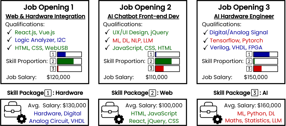
Figure 1. An illustrative example on skill-salary influence.

To tackle these challenges, we propose a novel, intrinsically explainable set-based neural prototyping approach, namely Local-Global Subset DisEntangling Set Network, called LGDESetNet, which models outcomes based on learning multi-faceted input subsets and influential prototypical sets. With LGDESetNet, we realize explainable and accurate salary prediction while disentangling salary-influential skill sets from both an instance-based local view and a task-based global view. In particular, to learn symbolic set influence, LGDESetNet models discrete and permutation-invariant set-formed patterns in a differentiable end-to-end manner. Specifically, we propose a disentangled discrete subset selection layer to identify local subsets reflecting different semantics. In particular, an element co-occurrence graph density regularization is designed for enhancing dense and disentangled extraction. Next, we propose a set-oriented discrete prototype learning method to extract globally influential sets, which generates outputs in a transparent way based on the semantic interactions between the extracted subsets and global prototypes. To flexibly process external job contexts (e.g., time, city), we design two optional fusion layers to integrate skill-wise and set-wise side information in an explainable way. Finally, we conduct extensive experiments on four real-world job salary datasets. The experimental results clearly show that LGDESetNet outperforms state-of-the-art self-explainable models and salary prediction models. Quantitative and qualitative analyses underscore our method’s superior explainability ability to identify influential skill sets in the labor market and quantify their impact on salaries.

Our key contributions are summarized as follows: 1) We provide a novel neural framework to effectively disentangle and quantify skill sets’ influence on salary from job posting data. 2) To the best of our knowledge, we are the first to develop a self-explainable deep set model that provides outcome-influential set-viewed explanations. 3) We propose a novel graph-enhanced subset selection layer and set-oriented prototypical learning method for distilling local and global influential skill sets. 4) Extensive experiments on real-world datasets, including a user study, present our model’s superior salary prediction performance alongside novel explainability capability.

2. Related Work

This paper’s related work falls into three categories: data-driven salary prediction, set modeling, and neural network explainability. We will discuss each category in detail and highlight the differences between our work and existing studies.

2.1. Data-driven Salary Prediction

In recent years, growing efforts have been made to explore salary-influential factors from a data-driven perspective (Quan and Raheem, 2022). Despite examining various factors (Autor and Dorn, 2013; Dix-Carneiro and Kovak, 2015; Burstein and Vogel, 2017; Sun et al., 2025), quantitative salary prediction remains challenging. The evolution of machine learning offers promising solutions for dynamic and effective salary prediction. For example, Lazar et al. (Lazar, 2004) adopted the classical Support Vector Machine (SVM) on talent demographics data to predict incomes. Meng et al. (Meng et al., 2018) proposed a holistic matrix factorization approach for salary benchmarking based on company and job position information. Meng et al. (Meng et al., 2022a) further designed a nonparametric Dirichlet process to capture the latent skill distributions. In (Sun et al., 2021), a cooperative composition deep model is introduced for salary prediction by market-aware skill valuation. Fang et al. (Fang et al., 2023) developed a pre-training method for recruitment tasks, achieving BERT-comparable performance in the downstream salary prediction task. Unlike existing works, our study focuses on the skill composition effect on job salary and proposes a self-explainable deep set model to provide explainable insights into skill-based salary-influencing patterns. Moreover, we holistically consider both local and global job contexts’ influences (e.g, skill proficiency, base city) on skill-salary prediction.

2.2. Set Modeling

In data mining, frequent pattern mining (Li et al., 2022) is used to discover frequently appearing sets within datasets. Neural network-based methods face challenges with set-structured inputs due to their unordered nature. DeepSets (Zaheer et al., 2017) is the prominent work, which proposed a unified framework based on the set-pooling method to compress any unordered set into a single embedding vector. Based on this framework, (Murphy et al., 2018) designed a learnable Janossy pooling layer to enhance the model flexibility. Another research line investigated the attention mechanism to discover the interactions between set elements (Lee et al., 2019; Maron et al., 2020; Hirsch and Gilad-Bachrach, 2021). SetNorm (Zhang et al., 2022b) further proposed a novel set normalization to increase model depths. Some domain-specific studies can be also viewed as special cases of learning sets, including point cloud (Qi et al., 2017; Xu et al., 2018; Wu et al., 2024; Chen et al., 2024), graphs (Maron et al., 2018; Kim et al., 2022), hypergraph (Chien et al., 2021) and images (Yao et al., 2024; Gordon et al., 2019). However, few studies have focused on explaining the set-based modeling process. The closest work to ours is Set-Tree (Hirsch and Gilad-Bachrach, 2021), which provides instance-wise explanations by measuring the frequency each item occurs in the attention-sets. In contrast, our work provides both multi-faceted local explanations and global prototypical examples with explicit quantitative importance weights.

2.3. Neural Network Explainability

Neural network explainability aims to uncover important local or global data patterns for model predictions (He et al., 2024; Li et al., 2024; Guo et al., 2025; Li et al., 2025). One research line is post-hoc explainability, which employs additional models like gradient-based (Selvaraju et al., 2017; Ancona et al., 2017) and perturbation-based (Lundberg and Lee, 2017) methods to explain black-box models. However, such post-hoc methods fail to provide intrinsic model insights in many cases (Rudin, 2019; Schröder et al., 2023; Sundararajan et al., 2017). Another approach is building self-explainable models, leveraging regularization (Lemhadri et al., 2021; Li et al., 2024) or attention mechanisms (Miao et al., 2022) to identify critical input patterns. Moreover, some explored prototype learning (Chen et al., 2019) or case-based reasoning (Kolodner, 1992), mimicking human problem-solving by matching representative examples (Van Gog and Rummel, 2010). PrototypeDNN (Li et al., 2018) and ProtoPNet (Chen et al., 2019)are pioneering works in prototype-based image classification. Subsequent work (Ma et al., 2024; Wang et al., 2021; Rymarczyk et al., 2021; Pach et al., 2025) aims to make explanations more concise and understandable. Prototype learning has been applied to sequences (Ming et al., 2019; Hong et al., 2020; Rajagopal et al., 2021), graphs (Zhang et al., 2022a; Seo et al., 2024; Dai and Wang, 2025), imitation learning (Jiang et al., 2023), traffic flow (Fauvel et al., 2023), and reinforcement learning (Sun et al., 2025; Kenny et al., 2022). As aforementioned, explaining the set-based modeling process remains underexplored. This work focuses on processing set-structured data by disentangling and prototyping relationships among set entities.

Table 1. Major notations in this paper.

Symbol	Description
$X$	The input skill set.
$x_{i}$	The $i$-$th$ skill in the skill set $X$.
$lv_{i}$	The skill-wise external information of the skill $x_{i}$.
$C$	The set-wise external information (job context).
$Y$	The salary outcome.
$U$	The universal set of all the appeared skills.
$N_{total}$	The total number of all appeared skills.
$E_{total}$	The embedding table of all appeared skills.
$\phi$	The skill encoding function.
$H$	The number of views.
$\alpha^{\text{lv}}_{i}$	The skill-wise importance weight of the skill $x_{i}$.
$S_{h}$	The $h$-th extracted subset.
$E^{\text{s}}_{h}$	The embeddings of the $h$-th subset.
$G_{skill}$	The skill co-occurrence graph.
$P_{i}$	The $i$-$th$ prototype.
$M$	The number of prototypes.
$\gamma^{\text{s}}_{i}$	The multi-hot selection vector of the prototype $P_{i}$.
$\gamma^{\text{lv}}_{i}$	The skill-wise weights of the prototype $P_{i}$.
$\gamma^{\text{sal}}_{i}$	The salary effect weight of the prototype $P_{i}$.
$E^{\text{p}}_{i}$	The continuous embeddings of the prototype $P_{i}$.
$\mathcal{T}$	The transformation layer.
$Z^{\text{s}}_{h}$	The projected embeddings of the subset $S_{h}$.
$Z^{\text{p}}_{i}$	The projected embeddings of the prototype $P_{i}$.

3. Problem Formulation

We utilize real-world job posting data (Sun et al., 2023; Meng et al., 2022b). Each job posting consists of the job salary range and descriptive external information, such as company, city, time, and skill level requirements. To mine the interaction among skill compositions, we formulate each job posting as a tuple $(X,C,Y)$, where $X$ represents a skill set, $C$ represents set-wise external information (e.g., job contexts such as time, city), and $Y$ represents its salary outcome. In particular, $X$ is an unordered set of skills $X=\{x_{1},x_{2},...,x_{n}\}$, where $n$ indicates the number of skills. Each skill $x_{i}$ is drawn from a universal set $U$. $N_{total}=|U|$ indicates the total number of skills across the dataset. In many real-world scenarios, each skill $x_{i}$ is possibly associated with skill-wise external information $lv_{i}$ (e.g., proficiency level).

Formally, we define the task of this paper as a skill-based explainable salary prediction problem. Using training data, it aims to train a neural network model $f$ that can predict salary outcomes based on skill sets with associated external information and provides explainable insights into the reasoning process. Additionally, $f$ should be permutation invariant for set processing, implying that $f(X)=f(\pi(X))$ for any permutation $\pi$ of the indices ${1,2,\ldots,|X|}$ and all $X$ in the input domain. Table 1 summarizes the major notations used in this paper.

4. Methodology

In this section, we first present the overview of LGDESetNet. Then, we introduce the details of each module and our training procedure for efficient set-oriented prototype learning.

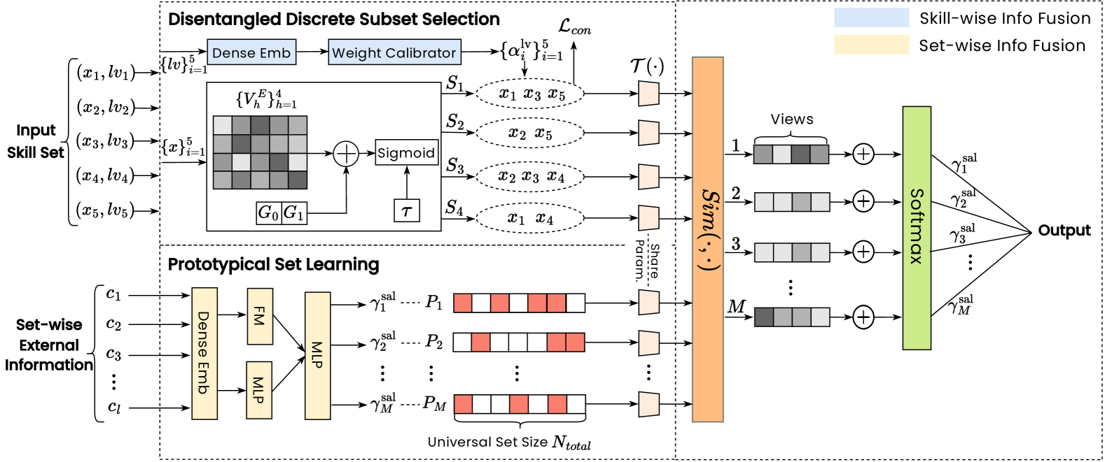
Figure 2. The architecture of LGDESetNet.

4.1. Framework Overview

As illustrated in Figure 2, the LGDESetNet model consists of two main components: disentangled discrete subset selection and prototypical set learning. Our model aims to provide explainable salary prediction by disentangling and quantifying the influence of skill sets on salaries from both local and global perspectives. To symbolize the collective semantic factors, LGDESetNet learns $M$ global representative skill compositions as prototypes $\{P_{1},P_{2},..,P_{M}\}$, each represented as a set of skills. Each prototype has specific semantics reflected by a cluster of influencing skill subsets on the market and has independent effects on salaries varying across different job contexts. Given an input skill set, which can reflect multiple views of skill compositions, LGDESetNet identifies $H$ key subsets $\{S_{1},S_{2},...,S_{H}\}$, representing diverse semantic views. These subsets are subsequently compared with global prototypes to determine pairwise similarity scores. The overall match of each prototype to the input is weighted and combined into the salary prediction.

To achieve this, the disentangled discrete subset module introduces a differentiable multi-view subset selection network. Through the Gumbel attention mechanism, it can explicitly represent each extracted subset as a discrete set instead of continuous embeddings. We further introduce a weight calibrator to measure the importance of each skill within the input set based on its external information. A co-occurrence graph density-based regularizer is proposed to encourage extracting semantically meaningful skill subsets. To symbolize global semantics, the prototypical set learning module employs a set-oriented prototypical part layer with an efficient embedding-projection training algorithm. This strategy enables learning discrete skill sets that align the distribution of local semantics of key subsets recognized from the inputs. We also introduce a contextual salary influence module to dynamically capture the varied salary effects of each prototype under different job contexts. Notably, the skill-wise and set-wise fusion layers are optional and can be flexibly integrated based on external job contexts.

4.2. Disentangled Discrete Subset Selection

The disentangled discrete subset selection component comprises a differentiable multi-view subset selection network, a skill-wise weight calibrator, and co-occurrence graph density regularization.

4.2.1. Multi-view Subset Selection Network

As demonstrated in our motivating example, real-world samples can reflect multiple skill semantics that influence the outcome from different views. In this case, regular prototype-based methods that learn representative patterns from the entire input space can reduce the model’s performance and obscure the model’s explainability by conflating semantics. To address this limitation, LGDESetNet disentangles the input into multiple subsets as its multi-view representations.

First, LGDESetNet uses a permutation-invariant encoder to embed each set’s overall semantic features. The input skill vector $V_{X}\in\mathbb{R}^{n}$ can be in any permutation order of inner skills, where $n$ denotes the size of $X$. The representation $\phi(x_{i})$ for each skill in $U$ is learned as an embedding table $E_{total}\in\mathbb{R}^{N_{total}\times d}$, where $d$ represents the embedding dimension. Next, a permutation-invariant pooling function $\text{pool}(\cdot)$ aggregates the input set’s skill representations into the set representation. We introduce the attention mechanism to capture the interactions of skills to different semantics, the skill and set’s representations are projected into $H$ distinct subspaces. For the $h$-th view, each row in $V_{h}^{\text{K}},V_{h}^{\text{V}}\in\mathbb{R}^{n\times d_{h}}$ denotes the key and value vectors of the corresponding skill in $V_{X}$, and $V_{h}^{\text{Q}}\in\mathbb{R}^{d_{h}}$ denotes the query projected from the set embedding. Using the dot-product attention mechanism (Vaswani et al., 2017), we calculate the similarity of each skill in each view as:

(1) $$V^{\text{E}}_{h}=V_{h}^{\text{Q}}(V_{h}^{\text{K}})^{T}/\sqrt{d_{h}}.$$

Each entry $V^{\text{E}}_{h}\in\mathbb{R}^{N}$ models a skill’s interaction with the $h$-th view.

While activation functions can be used to project interaction weights to the range [0, 1], the continuous interaction score hinders the network’s ability to model in an explicit binary manner. To address this issue, we introduce Gumbel-Sigmoid (Gumbel, 1948; Geng et al., 2020) to enable differentiable skill selection. Specifically, we incorporate Gumbel noise with the Sigmoid function and output the selected skills for each view’s subset as:

(2) $$\begin{split}A^{\text{s}}_{h}=\frac{\exp((V^{\text{E}}_{h}+G_{0})/\tau)}{\exp((V^{\text{E}}_{h}+G_{0})/\tau)+\exp((G_{1})/\tau)},\\ u_{i}\sim\text{Uniform}(0,1),i\in\{0,1\},\\ G_{i}=-\log(-\log(u_{i})),i\in\{0,1\},\end{split}$$

where $G_{0}$ and $G_{1}$ are two i.i.d Gumbel noises, the temperature $\tau$ controls the smoothness of the sampling function. $A^{\text{s}}_{h}$ becomes a multi-hot vector for selecting a subset $S_{h}$ when $\tau$ approaches $0$ and becomes a continuous vector as $\tau\rightarrow\infty$. In the training loop, we gradually reduce $\tau$ to learn the multi-hot representation.

4.2.2. Skill-wise External Information Fusion

In practice, skills are usually associated with external information, offering nuanced insights into its impact on salary determination. For instance, while “Algorithms (Understand)” and “Algorithms (Specialist)” share identical skill semantics, the latter likely exerts a greater influence within the skill set. This motivates us to design a weight calibrator for explicitly modeling these skill-wise dynamic relationships. We adjust the weights of each skill’s embeddings to discern the varied importance of skills within a set while preserving original skill semantics. Specifically, we learn the dense embeddings from the external information $lv_{i}$ of the skill $x_{i}$ and project it into a weight value $\alpha^{\text{lv}}_{i}$ ranging in $[0,1]$ with the Sigmoid function. In this way, we can get fused embedding $E^{\text{s}}_{h}$ of the extracted subset $S_{h}$ by integrating the skill embeddings weighted by their skill-wise importance before the pooling operation:

(3) $$\begin{split}E^{\text{s}}_{h}&=\text{pool}\left(\{\alpha^{\text{lv}}_{i}\phi(x_{i})|x_{i}\in S_{h}\}\right).\end{split}$$

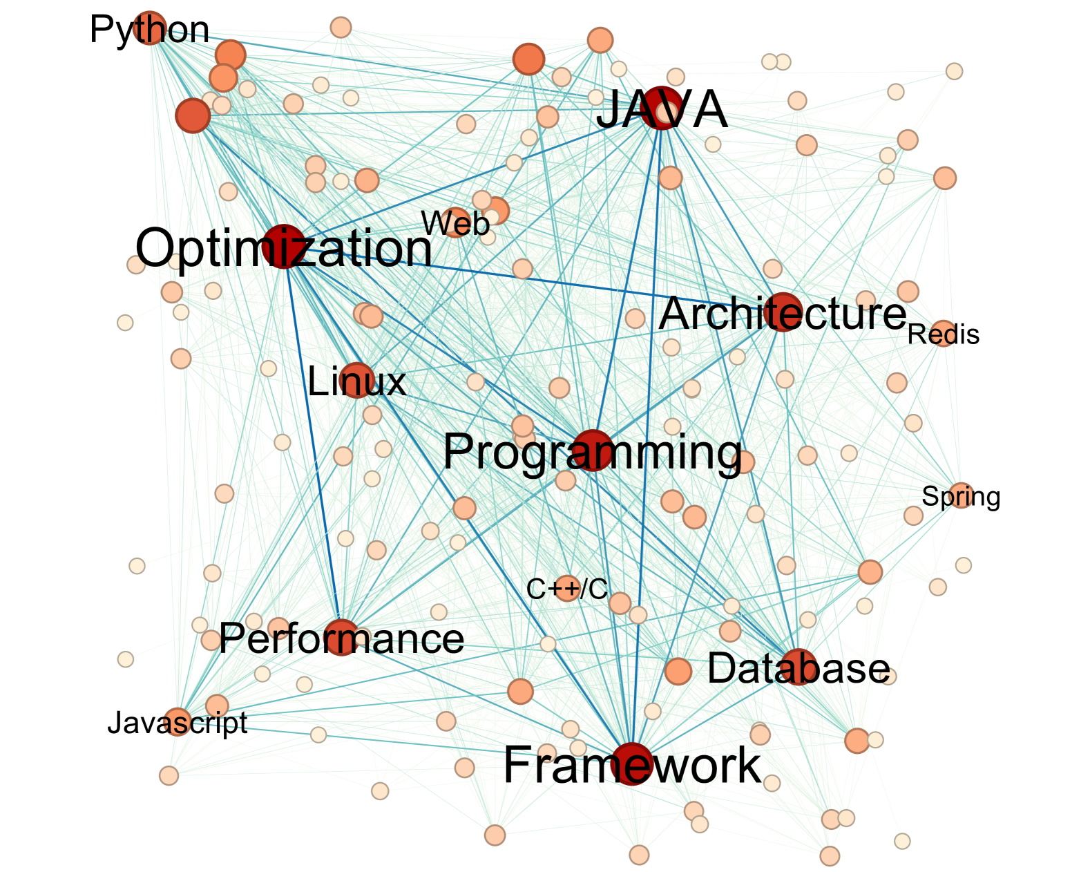
(a) IT

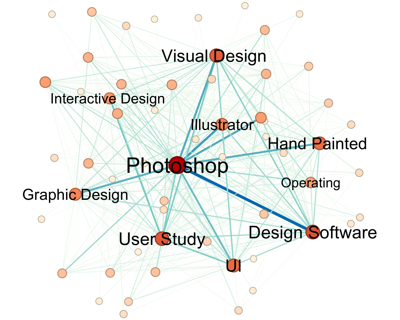
(b) Designer

Figure 3. Illustrative examples of co-occurrence graphs. Low-weight edges are eliminated to ease presentation.

4.2.3. Co-occurrence Graph Density Regularization

To enhance explainability and robustness, extracted skill subsets should reflect meaningful real-world interactions. Yet, focusing solely on prediction performance could generate subsets cluttered with irrelevant skills, reducing semantic clarity. To address this, we introduce a regularization approach aimed at refining these subsets to meet key intuitive criteria: (i) Semantic coherence within subsets, (ii) Distinct semantic boundaries between different subsets, and (iii) Avoidance of trivial subset selections (neither fully inclusive nor empty sets).

Observing that skills frequently appeared together in job postings likely share semantic connections (e.g., “Machine Learning”, “Algorithms”, and “Python” often cluster in AI roles), we leverage global semantic interactions inferred from such co-occurrence patterns. Direct co-occurrence analysis, however, is computationally expensive and hampered by data sparsity. Therefore, we model these relationships using a skill co-occurrence graph $G_{skill}=\langle U,L\rangle$, drawing from skill pair associations across the dataset, where $U$ is the universal set of skills and $L$ represents the links indicating co-occurrence frequencies between skill pairs. As exemplified in Figure 3, each graph node corresponds to a skill, and a link $l_{i,j}$ between nodes $x_{i}$ and $x_{j}$ signifies their connectivity, quantified by their co-occurrence frequency $w_{l_{i,j}}$. To quantify semantic connections within subsets, we design a graph density-based (Khuller and Saha, 2009) regularization, focusing on the subgraph $G_{h}=\langle S_{h},L_{G_{h}}\rangle$ for each subset $S_{h}$. The subgraph’s density, calculated as $\frac{\sum_{l\in L_{\mathrm{G}_{h}}}w_{l}}{|L_{{\mathrm{G}_{h}}|}}$, gauges the semantic cohesiveness of the subset. By maximizing this density, we encourage subsets that are semantically well-connected, while minimizing trivial or overly inclusive selections. Our graph regularization of the extracted subsets $\{S_{h}\}_{h=1}^{H}$ is thus defined as:

(4) $$\mathcal{L}_{con}=-\log\frac{1}{H}\sum_{h=1}^{H}\frac{\sum_{l\in L_{\mathrm{G}_{h}}}w_{l}}{|L_{\mathrm{G}_{h}}|}.$$

This approach not only ensures subsets are semantically dense but also supports the network’s focus on enhancing performance without losing critical information through subset disentanglement.

4.3. Prototypical Set Learning

Based on extracted subsets, LGDESetNet matches the input with learnable prototypes representing global semantics and accordingly models the output as an aggregation of these global contributions.

4.3.1. Set-oriented Prototypical Part Layer

The prototypical part network learns $M$ input-independent prototypical skill sets $\{P_{i}\}_{i=1}^{M}$. To provide an explicit skill set semantic, we adopt an approach distinct from conventional embedding-based prototype learning. Specifically, we utilize a discrete multi-hot vector to represent the prototypes, denoted as $\gamma^{\text{s}}\in\{0,1\}^{M\times N_{\text{total}}}$. Each row $\gamma^{\text{s}}_{i}\in\{0,1\}^{N_{\text{total}}}$ indicates a prototype’s multi-hot vector and its inner entries show if a skill is contained. Considering a global semantic may involve skills with different importance in practice, a weight vector $\gamma^{\text{lv}}_{i}\in[0,1]^{N_{\text{total}}}$ is associated with each prototype, indicating each skill’s importance within the prototype. The differentiable training procedure of set-oriented prototypes will be detailed in Section 4.3.4.

We assess the alignment between the input set and each prototype (i.e., global semantics) by comparing the similarity of extracted subsets to the prototypes. Notably, the discrete set representation brings the curse of dimensionality, complicating set similarity estimation. For instance, “C” and “C++” are treated as distinct skills despite their semantic closeness, potentially hindering model convergence and accuracy. To address this, we project prototype $P_{i}$ and subset $S_{h}$ into semantic representation vectors with the same skill embedding table as the input set, denoted as $E^{\text{p}}_{i}=\text{pool}\left(\{\gamma^{\text{s}}_{i}\gamma^{\text{lv}}_{i}\phi(x_{i})|x_{i}\in U\}\right)$ and $E^{\text{s}}_{h}=\text{pool}\left(\{\alpha^{\text{lv}}_{i}\phi(x_{i})|x_{i}\in S_{h}\}\right)$. Considering the distribution shift between the whole set and single-view subsets, we introduce a transformation layer $\mathcal{T}$ to further project the subsets and prototypes into a subset representation space as $Z^{\text{p}}_{i}=\mathcal{T}\left(E^{\text{p}}_{i}\right)$ and $Z^{\text{s}}_{h}=\mathcal{T}\left(E^{\text{s}}_{h}\right)$. In this way, we better capture semantic-level associations while ensuring the similarity can be measured by aligned representation of prototypes and subsets.

Finally, we calculate the pairwise similarity between a subset $S_{h}$ and a prototype $P_{i}$ as

(5) $$sim(S_{h},P_{i})=\text{log}\left(\frac{\|Z^{\text{s}}_{h}-Z^{\text{p}}_{i}\|_{2}^{2}+1}{\|Z^{\text{s}}_{h}-Z^{\text{p}}_{i}\|_{2}^{2}+\epsilon}\right).$$

For each prototype, we aggregate their similarity to different extracted subsets and apply softmax to obtain a global normalized similarity score. Moreover, each prototype is associated with a job-context-dependent weight value $\gamma^{\text{sal}}_{i}$, reflecting its salary effects in specific job contexts. We constrain these weight values as non-negative values to enhance explainability. Thus, the output can be modeled as the weighted average of the similarity scores between each prototype and the input skill set:

(6) $$y=\sum_{i=1}^{M}\gamma^{\text{sal}}_{i}\cdot\text{softmax}(\sum_{h=1}^{H}sim(S_{h},P_{i})).$$

4.3.2. Set-wise External Information Fusion

In practice, each skill set is enriched with set-wise external information, which is also useful in determining salary outcomes. For example, job salaries are highly correlated with the work experience and the pricing level of the base city. However, directly fusing such information into deep and wide embeddings (Cheng et al., 2016) could obscure the model’s explainability. Therefore, we separate the set-wise external information from skill embeddings, acknowledging that the salary effects of global prototypical skill sets may vary across different job scenarios. Specifically, we model this prototype salary effect dynamic as a function of the set-wise external features $C=\{c_{1},c_{2},...,c_{l}\}$. Drawing inspiration from DeepFM (Guo et al., 2017), we utilize a factorization machine encoder for low-order feature interactions and an MLP encoder for high-order interactions. By aggregating the embeddings from both encoders, we then employ another MLP to estimate the salary effects of each prototype, ensuring a dynamic and contextual assessment of skill sets’ impact on salary predictions:

(7) $$\begin{split}\gamma^{\text{sal}}&=\text{MLP}\left(\text{FM}(C)+\text{MLP}(c_{1}|c_{2}|...|c_{l})\right).\\ \text{FM}(C)&=w_{0}+\sum_{i=1}^{l}w_{i}c_{i}+\sum_{i=1}^{l}\sum_{j=i+1}^{l}c_{i}\odot c_{j},\end{split}$$

where $\odot$ denotes the element-wise multiplication between features.

4.3.3. Prototype Learning Regularization

To enhance explainability, we introduce regularization methods for our prototypical set learning procedure, whose basic ideas are widely adopted in prototype learning for other data structures (Zhang et al., 2022a; Ming et al., 2019). First, since prototypes are desired to be representative exemplars for the subsets, we introduce a representation regularization term to encourage each subset to be close to at least one prototype and encourage each prototype to be close to at least one extracted subset.

(8) $$\mathcal{L}_{rep}=\frac{1}{H}\sum\limits_{h=1}^{H}\min_{i\in[1,M]}\|Z^{\text{s}}_{h}-Z^{\text{p}}_{i}\|_{2}^{2}+\frac{1}{M}\sum_{i=1}^{M}\min_{h\in[1,H]}\|Z^{\text{s}}_{h}-Z^{\text{p}}_{i}\|_{2}^{2}.$$

Moreover, to learn an extensive prototypical embedding space, we introduce a diversity regularization term to scatter prototypes.

(9) $$\mathcal{L}_{div}=\frac{1}{M}\sum_{i=1}^{M}\sum_{j=i+1}^{M}\max(0,sim(P_{i},P_{j})-\theta_{min}),$$

where $\theta_{min}$ is a pre-defined threshold that verdicts whether a prototype pair is close or not. We set $\theta_{min}$ to $1.0$ in our experiments.

To summarize, the overall loss function is formulated as:

(10) $$\mathcal{L}=\mathcal{L}_{pred}+\lambda_{con}\mathcal{L}_{con}+\lambda_{rep}\mathcal{L}_{rep}+\lambda_{div}\mathcal{L}_{div}.$$

where $\mathcal{L}_{pred}$ is an appropriate loss function for outcome prediction and $\lambda_{*}$ are hyperparameters for controlling the impacts of regularization terms on model explainability.

Algorithm 1 Training Procedure of LGDESetNet

1:The dataset $\mathcal{D}=\{(X_{i},C_{i},Y_{i})\}_{i=1}^{N_{d}}$, Total number of epochs $N_{t}$, Warm-up epoch $N_{w}$, Prototype projection period $\tau$, and Prototype refinement epoch $N_{f}$;

2:Parameters of the trained model $\Phi$ and set-formed prototypical concepts $\{P_{k}\}_{k=1}^{M}$;

3:Initialize the model parameters $\Phi$;

4:Extract the frequent skill sets $\mathcal{D}_{S}$ from $\mathcal{D}$;

5:for Epoch $e$ = 1, 2,…, $N_{t}$ do

6:  Fit $\Phi$ on $\mathcal{D}$ by minimizing $\mathcal{L}$;

7:  if $e>N_{w}$ and $e\%\tau==0$ then

8:   Inference all the extracted subsets $\mathcal{S}$ using $\Phi$ on $\mathcal{D}_{S}$;

9:   for $k=1,2,...,M$ do

10:     $\gamma^{\text{s}*}_{k},\gamma^{\text{lv}*}_{k}\leftarrow\operatorname*{arg\,max}_{S\in\mathcal{S}}sim(S,P_{k})$

11:     $E^{p*}_{k}\leftarrow\text{pool}\left(\{\gamma^{\text{s}*}_{k}\gamma^{\text{lv}*}_{k}\phi(x_{i})|x_{i}\in U\}\right)$

12:   end for

13:  end if

14:end for

15:for $k=1,2,...,M$ do

16:  Initialize $\triangle E^{p}_{k}=\mathcal{T}\left(\text{pool}\left(\{\left(\gamma^{\text{s}*}_{k}\gamma^{\text{lv}*}_{k}+\triangle P_{k}\right)\phi(x_{i})|x_{i}\in U\}\right)\right)$;

17:  Freeze $E^{p*}_{k}$ and replace $E^{p}_{k}$ with $E^{p*}_{k}+\triangle E^{p}_{k}$;

18:end for

19:for $l=1,2,...,N_{f}$ do

20:  Fit $\Phi$ on $\mathcal{D}$ by minimizing $\mathcal{L}+\lambda_{p}\sum_{k=1}^{M}\|\triangle P_{k}\|_{1}$;

21:end for

22:$\{P_{k}\}_{k=1}^{M}\leftarrow\{\gamma^{\text{s}*}_{k}+\triangle P_{k},\gamma^{\text{lv}*}_{k}\}_{k=1}^{M}$;

23:return $\Phi$ and $\{P_{k}\}_{k=1}^{M}$;

Figure 4. Training procedure of LGDESetNet.

4.3.4. Embedding-Projection Training Procedure

Training discrete prototypes directly using gradient descent on randomly initialized values is challenging due to the non-contiguous nature of prototype representation. Direct L1 regularization could incur stringent constraints and adversely affect the model performance due to the skill sparsity. To address these limitations, we introduce an embedding-projection iterative learning algorithm for discrete prototypes. Algorithm 1 details the training procedure with Figure 4 graphically illustrating the workflow. The algorithm proceeds in five steps: (1) We start by optimizing the target embeddings $E^{\text{p}}$ for prototypes, updating them without back-propagating gradients to the discrete representations. Since $E^{\text{p}}$ is contiguous, gradient descent can effectively optimize it. This stage includes $N_{w}$ warm-up epochs to guide $E^{\text{p}}$ towards the appropriate semantic space. (2) Once retrieving the continuous prototype embeddings from the trained model, (3) we identify the closest matching subsets from frequent skill sets in the training data, (4) and then update the discrete prototypes and their corresponding embeddings $E^{\text{p}*}$. (5) Upon finalizing, we enhance the prototype’s adaptability by adding a minimal bias term to its discrete representation. Specifically, we freeze $E^{\text{p}*}$ and introduce a learnable bias term $\triangle E^{\text{p}}$, whose weight vector $\triangle P$ is initialized as zeros and L1-regularized. This fine-tuning step preserves explainability while allowing for nuanced expression of prototypical semantic uncertainty. To demonstrate the effectiveness of our architecture design for set-based modeling, we provide a theoretical proof of network permutation invariance in the Appendix A.

4.4. Complexity Analysis

We present a theoretical analysis of LGDESetNet’s computational complexity to demonstrate its feasibility for real-world deployment. The model’s time complexity is dominated by two primary components: the disentangled discrete subset selection module with complexity $O(n^{2}\times d\times H)$ for input sets of size $n$ with embedding dimension $d$ across $H$ views, and the prototypical set learning component requiring $O(H\times M\times d)$ operations for comparing extracted subsets with $M$ prototypes. Combined, the overall inference time complexity is $O(n^{2}\times d\times H+H\times M\times d)$, which remains manageable for typical skill set sizes. The quadratic dependency on input set size $n$ aligns with attention-based methods in set processing, including Set-Tree (Hirsch and Gilad-Bachrach, 2021) and SESM (Geng et al., 2020), and remains computationally feasible given the typically modest number of skills in real-world job postings. Importantly, our model’s linear scaling with respect to views ($H$) and prototypes ($M$) enables precise control over computational requirements and model capacity, allowing for effective deployment across various computational environments. For example, reducing $H$ decreases skill set selection costs, while limiting $M$ reduces prototype comparison operations. The skill/set-wise information fusion modules can be simplified to constant-time operations when external information is unnecessary, further optimizing computational requirements. These properties ensure LGDESetNet remains computationally efficient while preserving explainability across diverse applications.

Table 2. Detailed Dataset Features

Features	IT	Designer	High-tech	Financial
# Job Postings	212,676	18,588	128,346	45,394
# Skills	1374	138	203	385
Skill Level	✓	✓
City	✓	✓	✓	✓
Company Name	✓	✓
Company Size	✓	✓	✓	✓
Company Stage	✓	✓	✓
Industry	✓	✓	✓
Work Experience	✓	✓
Job Temptation	✓	✓
Time	✓	✓
Employer Type				✓

5. Experiments

Table 3. Overall performance evaluation. The listed methods include two categories: salary prediction models and self-explainable models. The best results are highlighted in bold.

Methods	Skill-Salary Job Postings (Sun et al., 2021)				Job Salary Benchmarking (Meng et al., 2022a)
	IT		Designer		High-tech		Finance
	RMSE ($\downarrow$)	MAE ($\downarrow$)	RMSE ($\downarrow$)	MAE ($\downarrow$)	RMSE ($\downarrow$)	MAE ($\downarrow$)	RMSE ($\downarrow$)	MAE ($\downarrow$)
HSBMF	$\text{5.291}_{\pm\text{0.017}}$	$\text{3.939}_{\pm\text{0.015}}$	$\text{4.612}_{\pm\text{0.025}}$	$\text{3.371}_{\pm\text{0.021}}$	$\text{3.844}_{\pm\text{0.016}}$	$\text{2.872}_{\pm\text{0.013}}$	$\text{4.299}_{\pm\text{0.025}}$	$\text{3.150}_{\pm\text{0.019}}$
SSCN	$\text{4.762}_{\pm\text{0.063}}$	$\text{3.484}_{\pm\text{0.052}}$	$\text{3.841}_{\pm\text{0.143}}$	$\text{2.766}_{\pm\text{0.102}}$	$\text{3.663}_{\pm\text{0.162}}$	$\text{2.740}_{\pm\text{0.106}}$	$\text{4.037}_{\pm\text{0.134}}$	$\text{2.948}_{\pm\text{0.096}}$
NDP-JSB	$\text{5.342}_{\pm\text{0.021}}$	$\text{4.073}_{\pm\text{0.021}}$	$\text{4.623}_{\pm\text{0.044}}$	$\text{3.262}_{\pm\text{0.023}}$	$\text{3.875}_{\pm\text{0.086}}$	$\text{2.827}_{\pm\text{0.067}}$	$\text{4.295}_{\pm\text{0.075}}$	$\text{3.146}_{\pm\text{0.071}}$
Set-Tree	$\text{5.552}_{\pm\text{0.065}}$	$\text{4.367}_{\pm\text{0.083}}$	$\text{4.339}_{\pm\text{0.149}}$	$\text{3.269}_{\pm\text{0.061}}$	$\text{3.953}_{\pm\text{0.092}}$	$\text{2.998}_{\pm\text{0.065}}$	$\text{4.406}_{\pm\text{0.079}}$	$\text{3.206}_{\pm\text{0.057}}$
SESM	$\text{4.489}_{\pm\text{0.034}}$	$\text{3.532}_{\pm\text{0.025}}$	$\text{3.812}_{\pm\text{0.123}}$	$\text{2.767}_{\pm\text{0.064}}$	$\text{3.623}_{\pm\text{0.029}}$	$\text{2.817}_{\pm\text{0.017}}$	$\text{3.967}_{\pm\text{0.031}}$	$\text{2.940}_{\pm\text{0.011}}$
ProtoPNet	$\text{4.503}_{\pm\text{0.029}}$	$\text{3.423}_{\pm\text{0.037}}$	$\text{3.794}_{\pm\text{0.013}}$	$\text{2.772}_{\pm\text{0.076}}$	$\text{3.602}_{\pm\text{0.110}}$	$\text{2.786}_{\pm\text{0.025}}$	$\text{4.116}_{\pm\text{0.144}}$	$\text{3.013}_{\pm\text{0.063}}$
TesNet	$\text{4.555}_{\pm\text{0.102}}$	$\text{3.698}_{\pm\text{0.037}}$	$\text{3.804}_{\pm\text{0.063}}$	$\text{2.902}_{\pm\text{0.012}}$	$\text{3.692}_{\pm\text{0.096}}$	$\text{2.806}_{\pm\text{0.081}}$	$\text{4.241}_{\pm\text{0.108}}$	$\text{3.094}_{\pm\text{0.071}}$
ProtoConcepts	$\text{4.468}_{\pm\text{0.062}}$	$\text{3.412}_{\pm\text{0.025}}$	$\text{3.792}_{\pm\text{0.083}}$	$\text{2.774}_{\pm\text{0.052}}$	$\text{3.504}_{\pm\text{0.061}}$	$\text{2.776}_{\pm\text{0.026}}$	$\text{4.023}_{\pm\text{0.034}}$	$\text{2.961}_{\pm\text{0.048}}$
LGDESetNet	${\text{4.162}_{\pm\text{0.012}}}$	${\text{3.141}_{\pm\text{0.041}}}$	${\text{3.473}_{\pm\text{0.058}}}$	${\text{2.559}_{\pm\text{0.062}}}$	${\text{3.327}_{\pm\text{0.038}}}$	${\text{2.434}_{\pm\text{0.037}}}$	${\text{3.775}_{\pm\text{0.046}}}$	${\text{2.768}_{\pm\text{0.031}}}$

5.1. Experimental Setup

5.1.1. Datasets

The data descriptions are provided in Section 3. We use four real-world, publicly available job posting datasets with distinct job and skill distributions: (1) Skill-Salary Job Postings datasets (Sun et al., 2023), including IT and designer topics. (2) Job Salary Benchmarking datasets (Meng et al., 2022b), covering high-tech and financial industries. We provide overview of detailed dataset features in Table 2, and provide more descriptive statistics in Appendix B.1.

5.1.2. Baseline Methods

We compare our LGDESetNet with the following state-of-the-art salary prediction models:

• HSBMF (Meng et al., 2018) is a salary benchmarking model utilizing a Bayesian approach to capture the hierarchical structure of job postings.

• SSCN (Sun et al., 2021) is an enhanced neural network with cooperative structure for separating job skills and measuring their values based on massive job postings.

• NDP-JSB (Meng et al., 2022a) develops a non-parametric Dirichlet process-based latent factor model to jointly model the latent representations of job contexts.

We also compare LGDESetNet with the following self-explainable models for set-based modeling.

• Set-Tree (Hirsch and Gilad-Bachrach, 2021) is a tree-based general framework for processing sets and quantifies the relative importance of each item according to its frequency.

• SESM (Geng et al., 2020) is an instance-wise selection method that discovers a fixed number of sub-inputs to explain its own prediction process.

• ProtoPNet (Chen et al., 2019) is the pioneering work in prototype-based models, which dissects the input for more fine-grained interpretation.

• TesNet (Wang et al., 2021) is another prototype-based image recognition deep network that introduces a transparent embedding space for disentangled global prototype construction.

• ProtoConcepts (Ma et al., 2024) modifies prototype geometry to enable visualizations of prototypes from multiple training images.

Specifically, directly applying SESM and prototype-based models is not viable due to the discrete and unordered nature of set data. To address this, we integrate the DeepSets framework and use LGDESetNet’s external information fusion method for fair comparison.

5.1.3. Implementation Details

We evaluate the performance based on RMSE/MAE for salary prediction tasks. All results are reported based on 5 rounds of experiments. The datasets are partitioned into training/validation/testing sets by a ratio of 6:2:2. For fair comparison, we select the hyperparameter configurations based on the best performance on the validation set. For all experiments, prototype number $M$ is set to 64 and head number $H$ is set to 4. The loss function hyperparameters $\lambda_{rep}$, $\lambda_{con}$, and $\lambda_{div}$ are all set to 0.1. We train our model with ADAM optimizer (Kingma and Ba, 2014). The transformation layer $\mathcal{T}$ is implemented using a 2-layer MLP layer with 256 hidden units. Experiments were implemented in Pytorch and run on a server with 8 Nvidia GeForce RTX 3090 GPUs. 

5.2. Overall Performance Evaluation

The overall prediction performance of LGDESetNet and all baselines on four datasets is reported in Table 3. We can observe that: (1) LGDESetNet consistently outperforms existing salary prediction baselines across all datasets, demonstrating that our comprehensive framework more effectively captures the complex factors influencing salary. This validates our hypothesis that a holistic skill set-based reasoning process can effectively model intrinsic salary-influential patterns. (2) Compared to self-explainable baselines, LGDESetNet achieves an average improvement of 10%. This substantial gain stems from our model’s ability to disentangle and prototype relationships among set entities while maintaining job context awareness, enabling more accurate identification of salary-influential skill patterns. Unlike existing self-interpretable models that often trade accuracy for explainability, LGDESetNet matches or even exceeds the performance of complex black-box models, as shown in Supplementary Table 6. This demonstrates its ability to bridge the typical performance gap between interpretable and black-box approaches, offering a more transparent yet accurate solution for set modeling. (3) The notable underperformance of Set-Tree compared to other methods highlights the importance of our approach. Set-Tree’s limitations in capturing job context-dependent nuances in set data and modeling combinatorial interactions among set elements underscore the challenges in explainable skill-based set modeling.

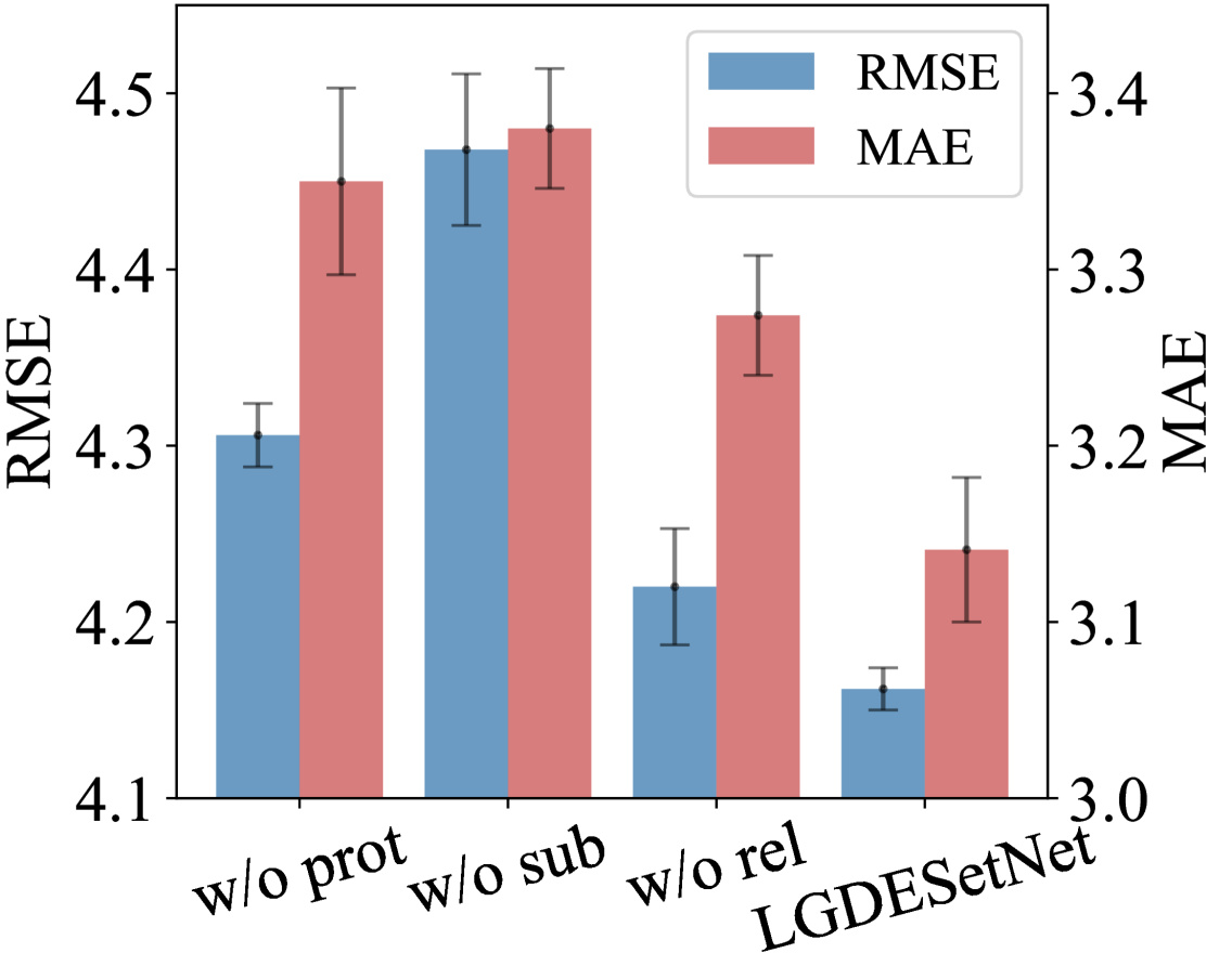
(a) IT

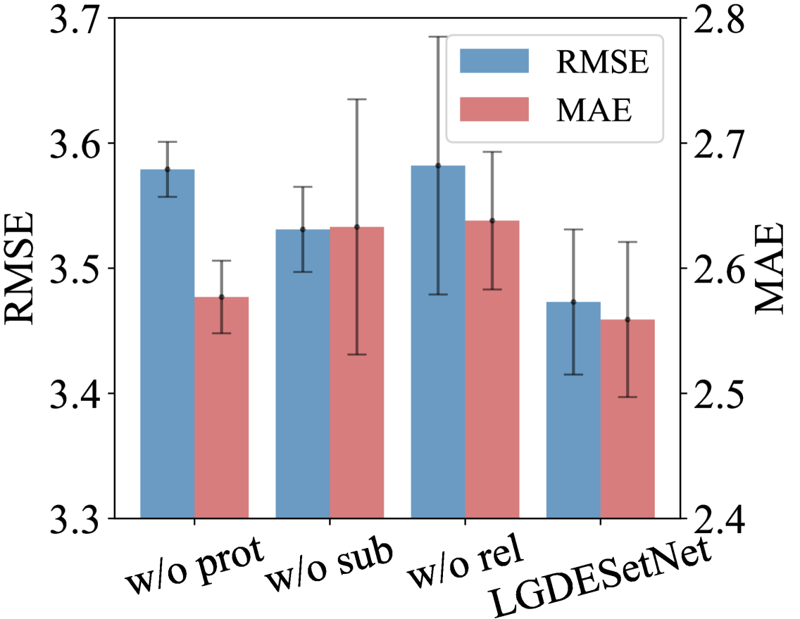
(b) Designer

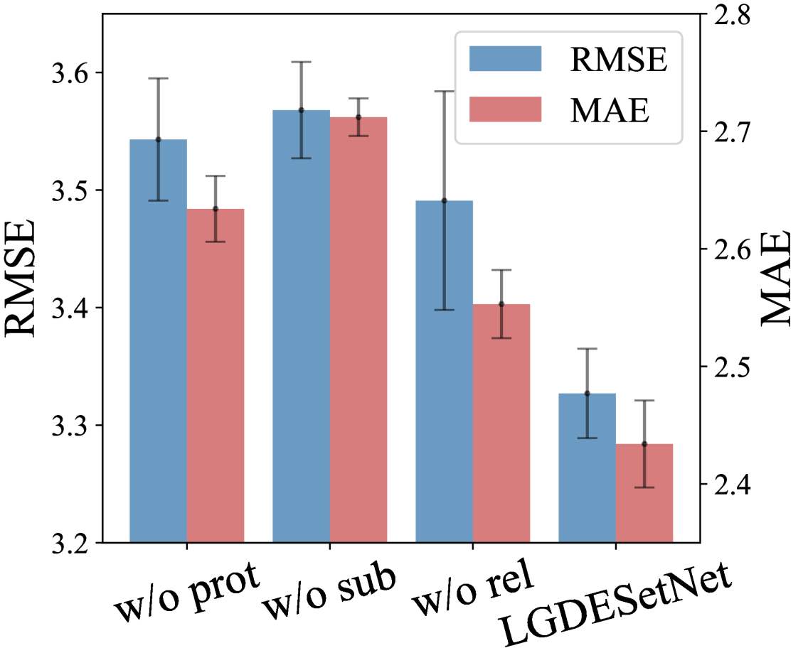
(c) High-tech

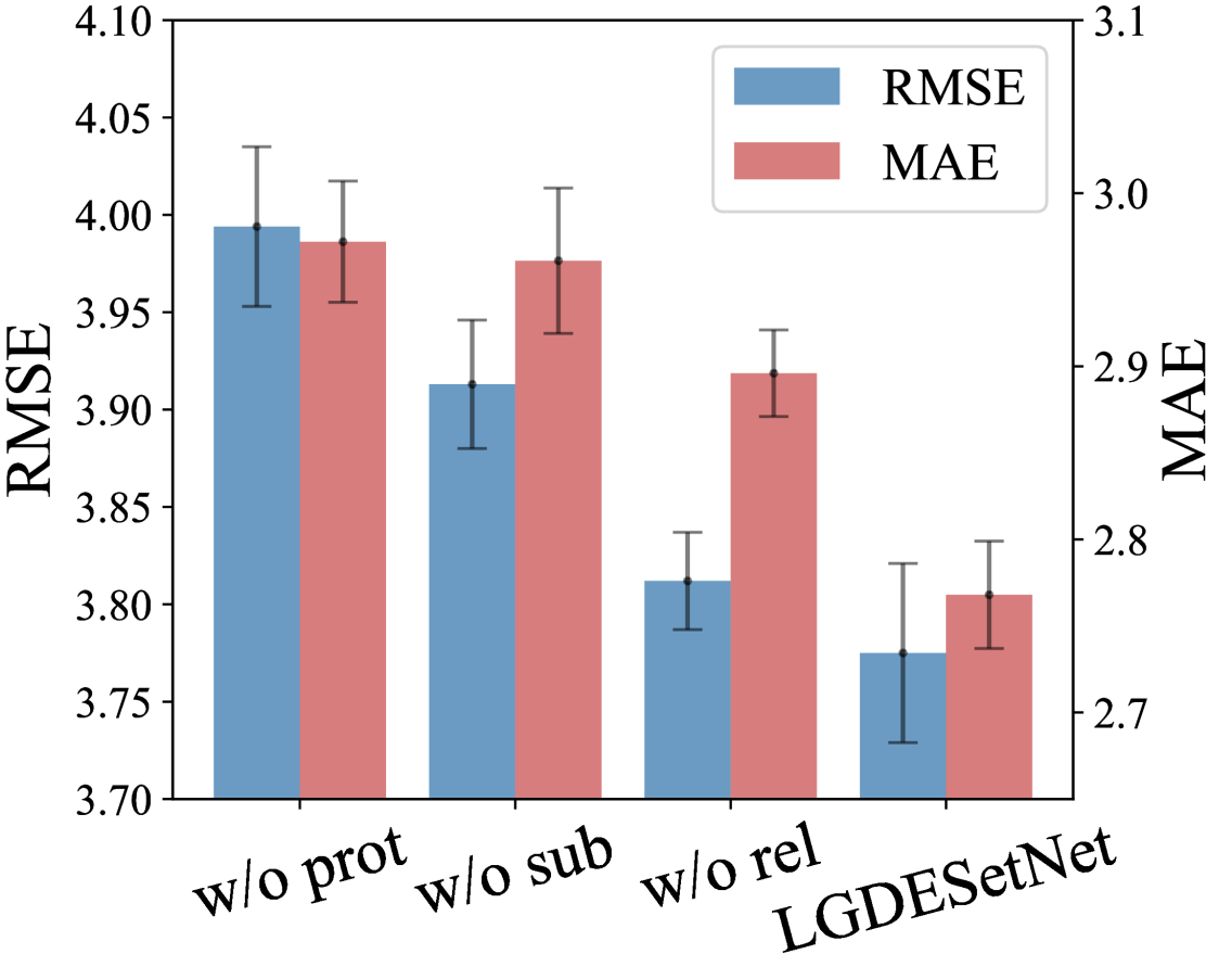
(d) Finance

Figure 5. Ablation studies on IT, Designer, High-tech, and Finance datasets.

5.3. Ablation Study

We introduce three variants of our LGDESetNet by disabling some parts of the network to evaluate the effectiveness of each component: (1) w/o prot, which disables the prototypical set learning module; (2) w/o sub, which disables the disentangled discrete subset selection module; and (3) w/o rel, which utilizes a conventional prototype replacement strategy (Ming et al., 2019) instead of our embedding-projection training algorithm. The results are reported in Figure 5. It can be observed that removing any modules from LGDESetNet reduces its performance, as the disentangled subset selection and prototypical learning modules are essential for capturing the full utility of set-valued reasoning. Particularly, the removal of the disentangled subset selection module leads to the most significant performance drop, underscoring the importance of skill semantic disentanglement. LGDESetNet outperforms these two components, which indicates that it not only raises the model explainability but also can increase the fitting ability by considering semantic interactions between subsets. Furthermore, LGDESetNet shows a 2%-5% performance gain over its variant with a classical projection strategy (Ming et al., 2019), validating our embedding-projection training’s effectiveness in advancing prototype learning.

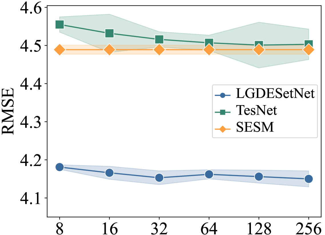
(a) Prototype Number $M$

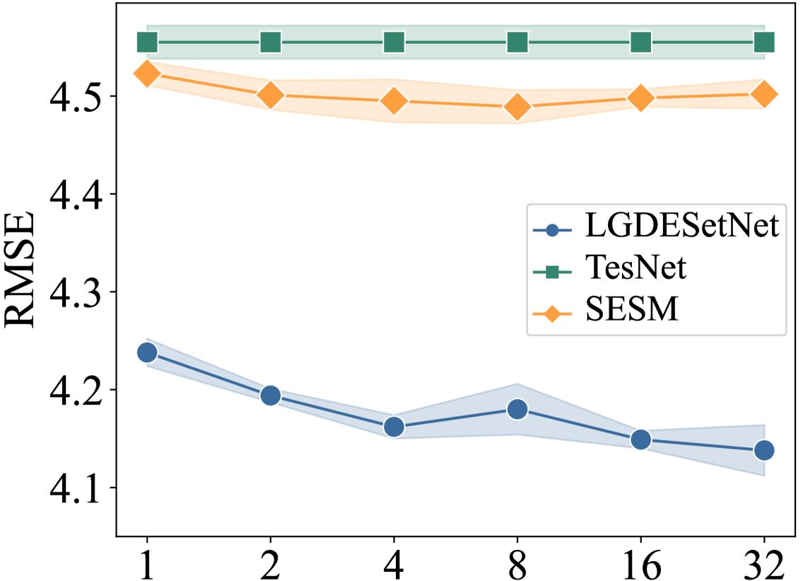
(b) View Number $H$

Figure 6. Parameter sensitivity of IT job postings.

5.4. Parameters Sensitivity

We further conduct the hyper-parameter analysis of the prototype number $M$ and the view number $H$. Specifically, we evaluate the performance of LGDESetNet with varying $M$ and $H$ on the IT dataset, compared with instance-wise selection model SESM (Geng et al., 2020) and prototype-based model TesNet (Wang et al., 2021). The results are shown in Figure 6. With the number of prototypes $M$ increases, the performance gets minorly better and stabilizes within a certain range. This pattern suggests that our model effectively captures the intrinsic dimensionality of the skill embedding space with a relatively small number of prototypes. Importantly, LGDESetNet maintains consistent performance advantages over baseline methods across all prototype settings, highlighting its inherent robustness to this hyperparameter. The stability plateau indicates that excessive prototypes may not necessarily improve the model’s performance, as they could introduce noise and redundancy. By default, we choose $M=64$ in order to get more diverse and representative skill prototypes.

The view number $H$ (Figure 6(b)) exhibits more pronounced sensitivity, with a steep performance improvement from $H=1$ to $H=4$, followed by marginal gains thereafter. This pattern reveals that multiple views are essential for capturing the multi-faceted nature of skill representations, but only up to a certain threshold. The rapid early improvement suggests that different views effectively capture complementary aspects of skill semantics. However, the diminishing returns beyond $H=4$ indicate a saturation point where additional views contribute minimal new information. Moreover, excessive view fragmentation can partition the semantic space too finely, potentially compromising both computational efficiency and interpretability. Based on this analysis, we adopt $H=4$ for our experiments as the optimal balance between model performance and semantic coherence.

Table 4. Results on subset cohesion score.

Methods IT Designer High-tech Finance SESM $\text{0.085}_{\pm\text{0.012}}$ $\text{0.035}_{\pm\text{0.018}}$ $\text{0.095}_{\pm\text{0.025}}$ $\text{0.074}_{\pm\text{0.023}}$ LGDESetNet $\text{0.126}_{\pm\text{0.034}}$ $\text{0.113}_{\pm\text{0.021}}$ $\text{0.186}_{\pm\text{0.011}}$ $\text{0.127}_{\pm\text{0.034}}$

5.5. Quantitative Explanation Analysis

We evaluate LGDESetNet’s ability to identify semantically cohesive skill subsets using the Subset Cohesion Score (SCS). SCS quantifies the semantic tightness of a subset $S$, calculated as $\text{SCS}(S)=\frac{2}{|S|(|S|-1)}\sum_{x_{i},x_{j}\in S}\mathcal{F}(x_{i},x_{j})$, where $\mathcal{F}$ indicates skill co-occurrence frequency across the dataset. As shown in Table 4, LGDESetNet substantially outperforms SESM across all four domains. These results demonstrate that our approach more effectively captures domain-specific skill relationships, with the greatest advantages observed in highly specialized fields where skill coherence is crucial. The consistent performance improvement across diverse domains indicates that LGDESetNet’s co-occurrence graph density regularization and global prototype-based selection mechanism successfully identify meaningful skill combinations rather than merely selecting individually relevant skills.

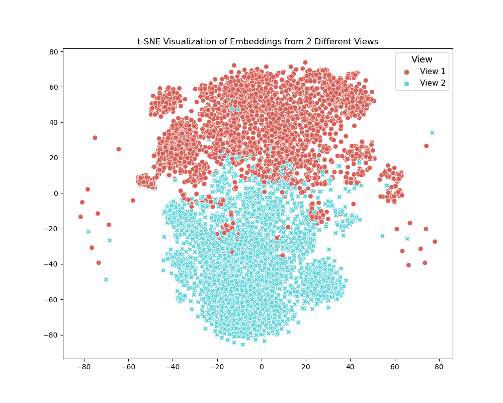
(a) $H=2$

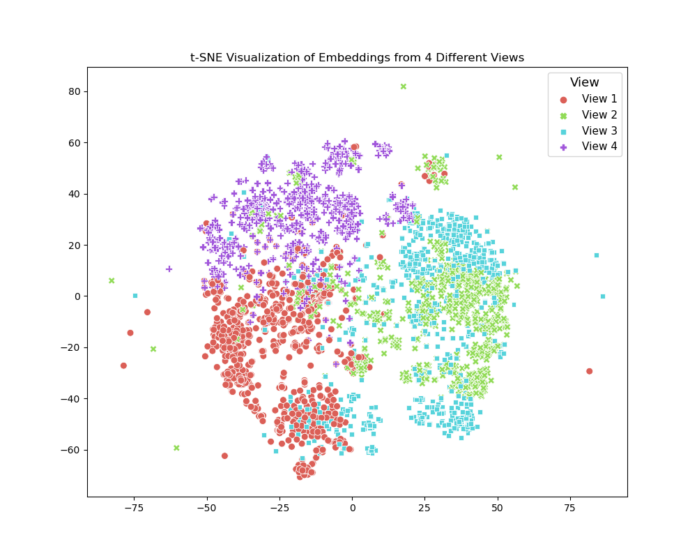
(b) $H=4$

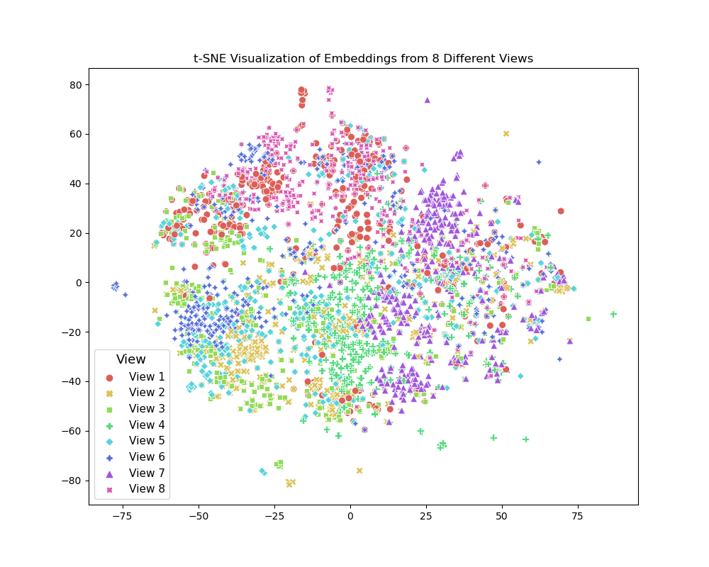
(c) $H=8$

Figure 7. t-SNE visualization of skill set embeddings with different view numbers $H$.

5.6. View Visualization

Figure 7 shows the t-SNE visualization of extracted skill subsets with different view numbers $H$. With $H$ = 2 or 4, we can observe that the skill embeddings are more compact and well-separated. Some overlap between views is reasonable, as certain skills share common traits, but the overall semantic meaning remains distinct. This indicates that LGDESetNet effectively captures the intrinsic skill relationships. When expanded to $H$ = 8, the skill embeddings become more dispersed, with less clear boundaries between different skill clusters. This suggests that excessive views may introduce redundancy, potentially compromising the model’s interpretability. This is also consistent with our previous experimental findings (shown in Figure 6(b)) that $H$ = 4 is the optimal balance.

(a) Top-5 Salary-Influential Prototypical Skill Sets

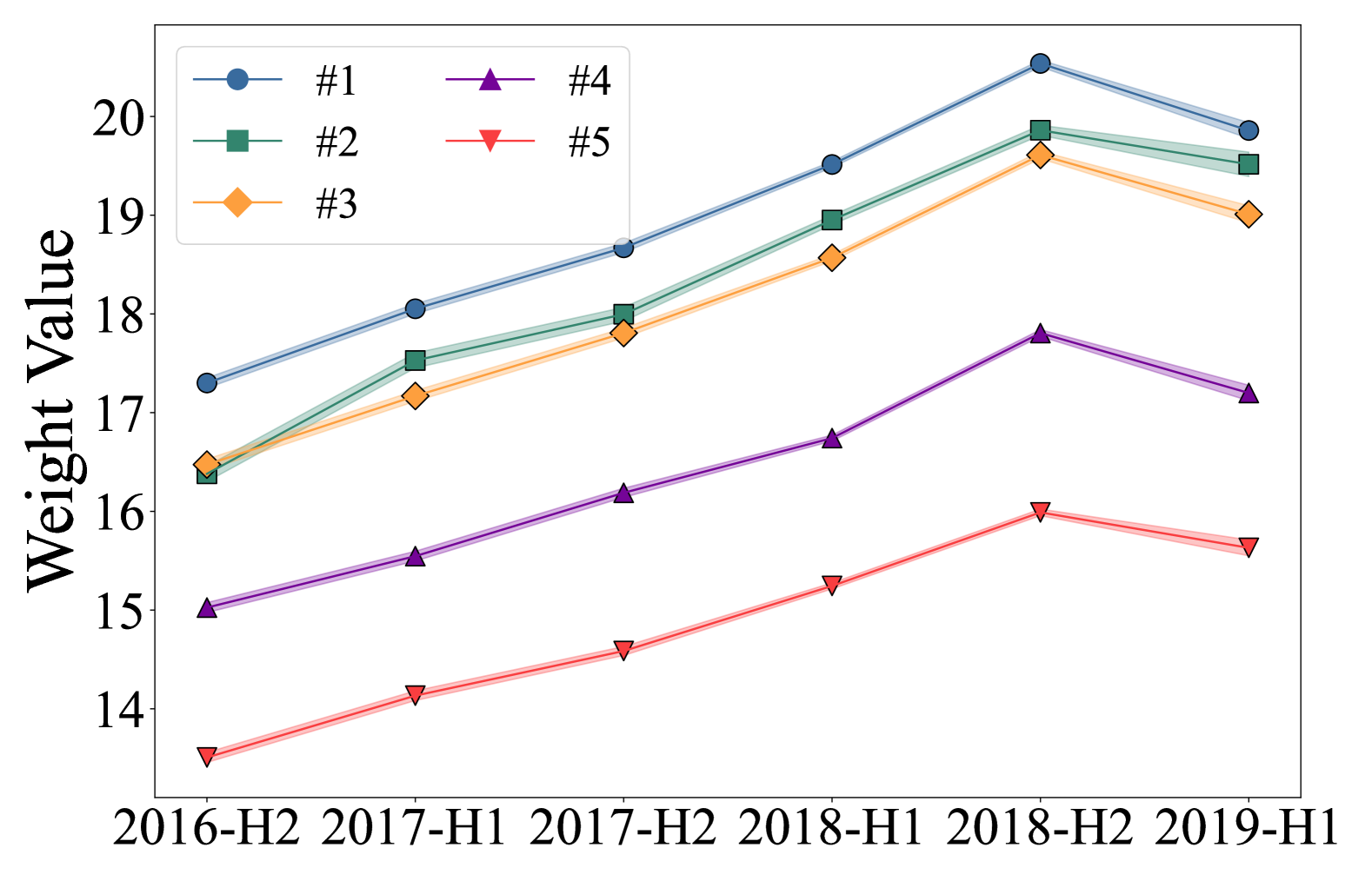
(b) Time

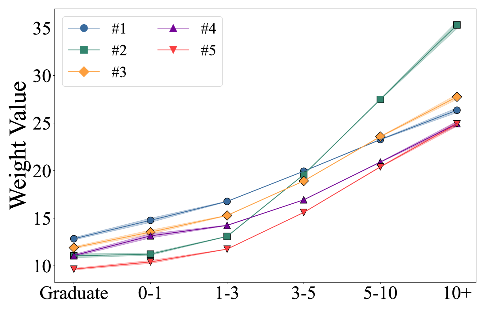
(c) Work Experience

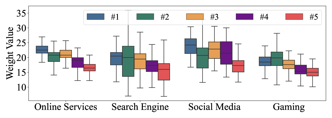
(d) Service Business

Figure 8. Global salary-influential prototypical skill sets concerning different job contexts.

5.7. Salary-influential Skill Set Analysis

5.7.1. Representative Skill Sets

As with our design, LGDESetNet models the combinatorial market-aware salary influences of skill compositions by learning the global prototypical skill sets. Figure 8(a) showcases IT-related skill sets with the top-5 highest average weights $\gamma^{\text{sal}}$ across the dataset. It illustrates LGDESetNet’s ability to highlight diverse job skills, ranging from software to hardware development. Furthermore, skill sets’ weight values indicate their market value for salary prediction, with AI and programming skills valued more than front-end skills, aligning with current labor market trends. By quantitative comparison with representative skill sets, talents can explicitly capture the labor market demands, identify skills gaps by comparison, and reasonably plan careers.

5.7.2. Skill Set Influence Concerning Different Job Contexts

We delve into the dynamic trends of prototypical skill sets across various job contexts, including time, work experience, and service business. By observing the fluctuations of prototype weight value, we can achieve many interesting insights into the labor market trends. From Figure 8(b), it’s evident that prototypical skill sets show an upward trend, highlighting an increasing demand for IT talents. Interestingly, there is a noticeable downturn in the first half of 2019, which is consistent with the global economic downturn’s impact. Figure 8(c) illustrates how work experience influences salary dynamics within job skill sets. For graduates, development-related skills could bring a higher initial salary. However, as work experience accumulates, the growth in salary slows down, hinting at a potential career ceiling. In contrast, algorithm-related skills demonstrate a more stable, enduring effect on salary progression. We also investigate the dynamic influences of service industry shown in Figure 8(d). For example, data analysis and backend development commanding higher median salaries due to their critical roles in managing and interpreting data, while hardware development is often underestimated by IT companies.

Figure 9. Reasoning processes of LGDESetNet on the IT-related job posting. LGDESetNet identifies semantically meaningful and disentangled subsets from the input set and thereafter provides representative subsets for evidence comparison.

5.8. Case study

In Figure 9, we qualitatively visualize LGDESetNet’s transparent reasoning process through a case study on a full-stack web development job posting. Initially, LGDESetNet identifies essential skill subsets from varied semantic angles—frontend, backend, machine learning, and interaction design. These extracted skill subsets are further compared with the global prototypical skill sets to calculate the similarities, which represents the corresponding semantic relevance. For example, the prototypical skill set {“Frontend Development”, “Framework”, “JavaScript”, “HTML”, “CSS”, “PHP”} has high similarity scores with the extracted subset 1, 2, and 4, which implies the high relevance of “Frontend Development” skills in the job posting. In the generalized additive aggregation module, these similarity scores are weighted and summed together to get a final predicted salary value. We can observe that LGDESetNet can highlight the most salary-influential patterns of skill sets. The skill topic “Frontend Development” primarily aligns with the input set that has the highest similarity scores. Moreover, it significantly influences salary prediction. While IT-related skills such as “Algorithms” and “Data Processing & Analysis”, can bring a high potential salary (high $\gamma^{\text{sal}}$), they have low relevance to web development and thereafter have fewer contributions to the outcome. This case study highlights LGDESetNet’s ability to clarify the salary reasoning process, with potential applications for various audiences. Recruiters may set equitable salaries, job seekers align skills with market trends, and policymakers inform education and workforce policies.

5.9. User Study

Following the design rationale of (Rong et al., 2023), we conduct a user study to evaluate LGDESetNet’s explainability by accessing the user’s comprehension of the model’s reasoning process (Understanding), their confidence and comfort with the recommendations (Trust), and the intuitiveness and ease of use of provided explanations (Usability). Specifically, we recruited 53 postgraduate students and staffs with the background of computer science or engineering from different universities for evaluation. We compare our network to a full black box (HSBMF), where people are simply told “a predicted result produced by a trained machine learning model” in text form, and a representative prototyping model (ProtoPNet), where the learned prototypical skill sets are presented as explanations. For fair comparison, all the designed questions stem from each model’s inherent modeling procedure. As shown in Table 5, We can observe that self-explainable models increase user confidence by providing the evidence of model inference. It shows the necessity of our efforts to qualify the impacts of job skills. Moreover, traditional prototyping methods fail to provide semantically dense skill sets, which might confuse and confound users. In contrast, LGDESetNet can enhance user experience by offering clear, separate skill compositions and using prototypical examples as comparative evidence.

Table 5. User study results: 5-point Likert scale ratings of three measured features for explanatory methods.

Methods HSBMF ProtoPNet LGDESetNet Understanding 3.742 3.927 4.421 Trust 3.385 3.521 4.220 Usability 3.046 4.028 4.623

6. Conclusion

In this study, we addressed the challenge of understanding how job skills influence job salaries. We introduced a novel intrinsically explainable set-based neural prototyping approach, LGDESetNet, to assess the impact of skill compositions on job salary, offering insights into disentangled skill sets influencing salary from a local and global viewpoint. Specifically, our approach leveraged a disentangled discrete subset selection module to pinpoint multi-faceted influential subsets with diverse semantics. In addition, we proposed a prototypical set learning method to distill globally influential skill sets. The final output transparently showcased the semantic relationships between these subsets and prototypes. Extensive evaluations on real-world datasets highlighted the effectiveness and explainability of LGDESetNet as a pioneering self-explainable neural methodology for processing skill-based salary prediction.

In this appendix, we provide the proof (Appendix A) of the permutation invariance of LGDESetNet. We also provide additional details on the dataset characteristics (Section B.1), and an additional case study (Section B.2).

Appendix A Proof of Permutation Invariance of LGDESetNet

Lemma 0.

(Permutation matrix and permutation function) $\forall X\in\mathbb{R}^{N\times N}$, for all permutation matrix $P$ of size $N$, there exists $\pi:\{1,2,...,N\}\rightarrow\{1,2,...,N\}$ is a permutation function, which satisfies:

$$X_{ij}=(PX)_{\pi(i)j}=(XP^{T})_{i\pi(j)}=(PXP^{T})_{\pi(i)\pi(j)}$$

Lemma 0.

Given $X\in\mathbb{R}^{N\times N}$ and any permutation matrix $P$ of size $N$, we have

$$\text{Sigmoid}(PXP^{T})=P\text{Sigmoid}(X)P^{T}.$$

Proof.

We have $\text{Sigmoid}(X)_{ij}=\frac{1}{1+e^{-X_{ij}}}$ and now consider the permutation function $\pi$ for $P$. Following the lemma 1, we can get:

$$\begin{split}(P\text{Sigmoid}(X)P^{T})_{\pi(i)\pi(j)}&=\text{Sigmoid}(X)_{ij}\\ &=\frac{1}{1+e^{-X_{ij}}}\\ &=\frac{1}{1+e^{-(PXP^{T})_{\pi(i)\pi(j)}}}\\ &=\text{Sigmoid}(PXP^{T})_{\pi(i)\pi(j)}.\end{split}$$

which implies $P\text{Sigmoid}(X)P^{T}=\text{Sigmoid}(PXP^{T})$. ∎

As presented before, we inject the Gumbel noises into the Sigmoid function for enabling a differentiable set element sampling process. Given a weight matrix $X$, this Gumbel-Sigmoid Sampler (GSS) can be formulated as:

$$\begin{split}\operatorname{GSS}(X)=\frac{\exp((X+G_{0})/\tau)}{\exp((X+G_{0})/\tau)+\exp((G_{1})/\tau)}.\end{split}$$

Lemma 0.

Given $X\in\mathbb{R}^{N\times N}$ and any permutation matrix $P$ of size $N$, we have

$$\operatorname{GSS}(PXP^{T})=P\operatorname{GSS}(X)P^{T}.$$

Proof.

Considering the GSS function only adds element-wise operations on Sigmoid, it does not change the original permutation property of Sigmoid. ∎

Proposition 1.

Given the input skill vector $V_{X}$ in any permutation order of the skill set $X$, the $h$-$th$ view of the multi-view subset selection network $\operatorname{MSSN}_{h}(V_{X})=\text{pool}\left(\operatorname{GSS}\left(V_{h}^{\text{Q}}(V_{h}^{\text{K}})^{T}/\sqrt{d}\right)\cdot V^{\text{V}}_{h}\right)$ is a permutation-invariant function.

Proof.

For the dot-product attention mechanism (Vaswani et al., 2017), we have $V_{h}^{\text{Q}}=V_{X}W^{\text{Q}}_{h}$, $V_{h}^{\text{K}}=V_{X}W^{\text{K}}_{h}$, and $V_{h}^{\text{V}}=V_{X}W^{\text{V}}_{h}$. Therefore, we can get

$$\begin{split}&\operatorname{MSSN}_{h}(PV_{X})\\ &=\text{pool}\left(\operatorname{GSS}(V_{h}^{\text{Q}}(V_{h}^{\text{K}})^{T}/\sqrt{d})V_{h}^{\text{V}}\right)\\ &=\text{pool}\left(\operatorname{GSS}(PV_{X}W^{\text{Q}}_{h}(PV_{X}W^{\text{K}}_{h})^{T}/\sqrt{d})PV_{X}W^{\text{V}}_{h}\right)\\ &=\text{pool}\left(\operatorname{GSS}(P(V_{X}W^{\text{Q}}_{h})(V_{X}W^{\text{K}}_{h})^{T}P^{T}/\sqrt{d})PV_{X}W^{\text{V}}_{h}\right)\\ &=\text{pool}\left(P\operatorname{GSS}((V_{X}W^{\text{Q}}_{h})(V_{X}W^{\text{K}}_{h})^{T}/\sqrt{d})P^{T}P(V_{X}W^{\text{V}}_{h})\right)\\ &=\text{pool}\left(P\operatorname{GSS}((V_{X}W^{\text{Q}}_{h})(V_{X}W^{\text{K}}_{h})^{T}/\sqrt{d})(V_{X}W^{\text{V}}_{h})\right)\\ &=\operatorname{MSSN}_{h}(V_{X})\end{split}$$

which implies the multi-view subset selection network is permutation-invariant by reason that the pooling function satisfies the property of permutation invariance. ∎

Proposition 2.

LGDESetNet satisfies the property of permutation invariance, that means given the input skill vector $V_{X}\in\mathbb{R}^{n}$ for any permutation matrix $P$ of size $n$, we can always have

$$\operatorname{LGDESetNet}(PV_{X})=\operatorname{LGDESetNet}(V_{X})$$

Proof.

Note that in LGDESetNet, we append a prototypical part network to the multi-view subset selection network. This network compares the extracted subsets with prototypes for weighted similarity aggregation. Since the prototyping operation is directly added to each subset embeddings $Z^{\text{s}}_{h}=\mathcal{T}\left(E^{\text{s}}_{h}\right)$, it does not change the permutation property of the multi-view subset selection network. Consequently, we can get that our LGDESetNet satisfies the permutation invariance condition. ∎

Appendix B Additional Experiments

B.1. Detailed Dataset Characteristics

To better understand the dataset characteristics, we provide detailed dataset statistics and analysis of frequent skill sets in Figure 10. It describes the skill and salary distributions of all four datasets. They present the unique characteristics of each dataset, such as the skill distribution and salary range. Moreover, we analyze the frequent skill sets (minSup $\geq$ 0.01) in the IT job posting dataset and present the salary distribution and Spearman correlation. The results show that the salary is significantly impacted by the skill sets, and the Spearman correlation indicates the co-appearance relationship of skill sets in job postings.

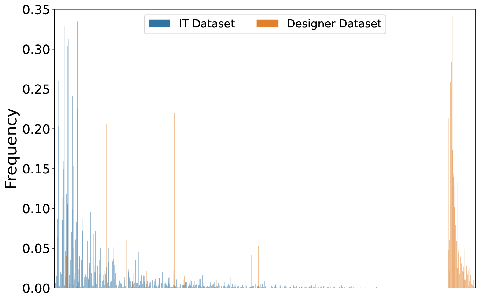
(a) Skill distribution

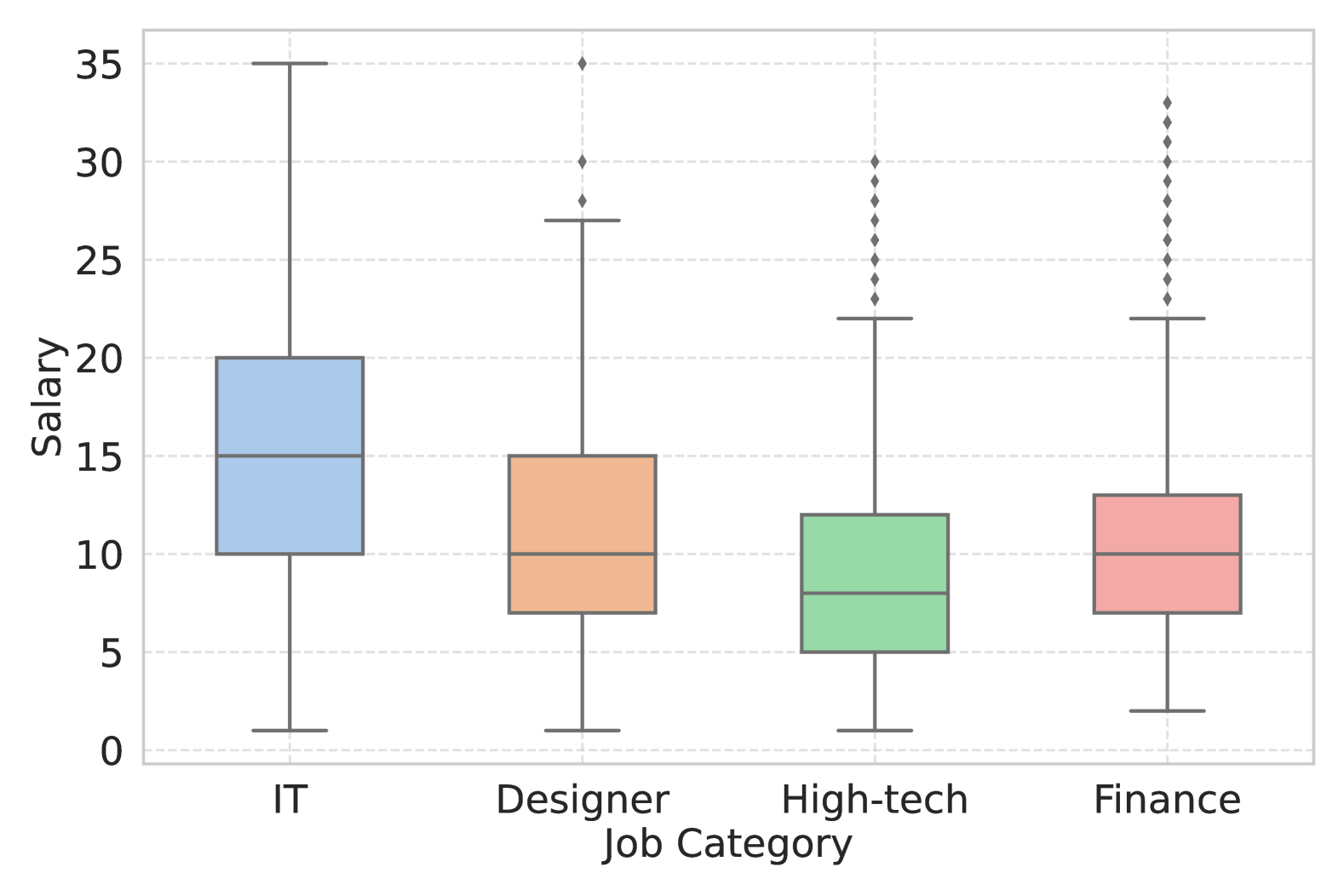
(b) Salary distribution

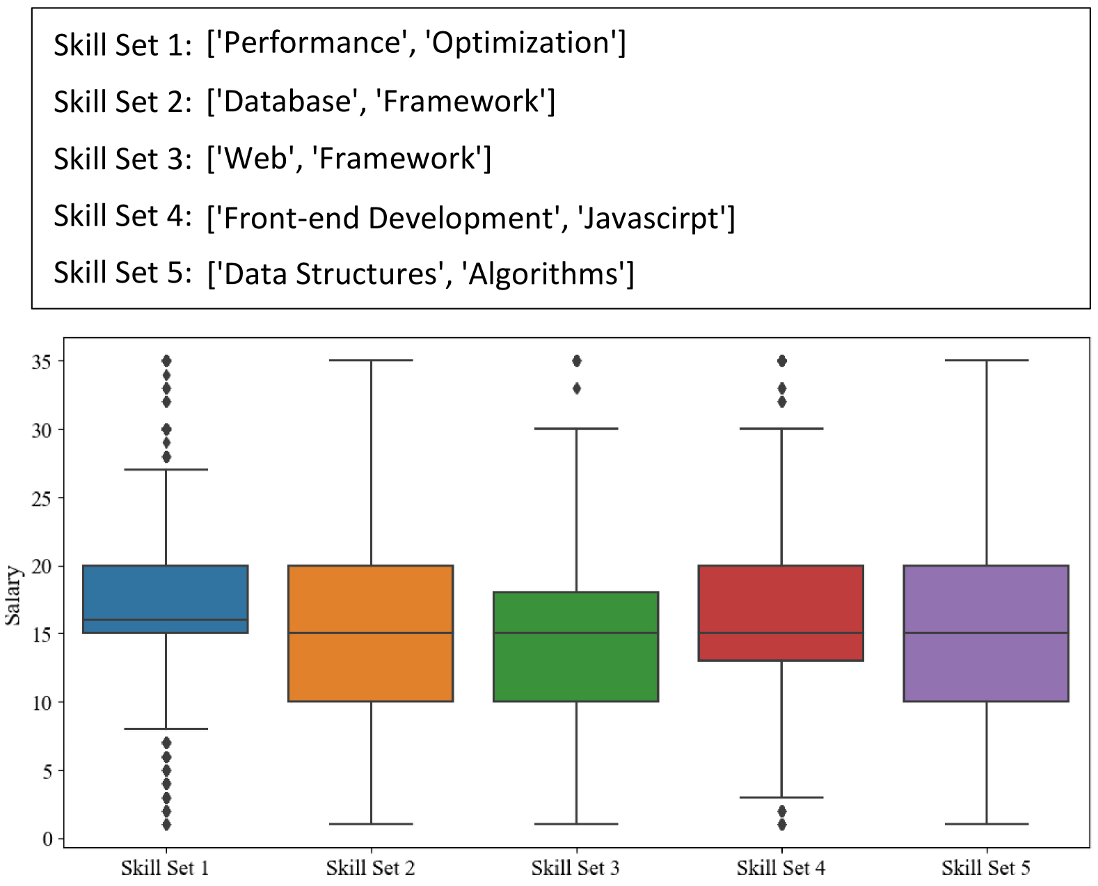
(c) Frequency analysis

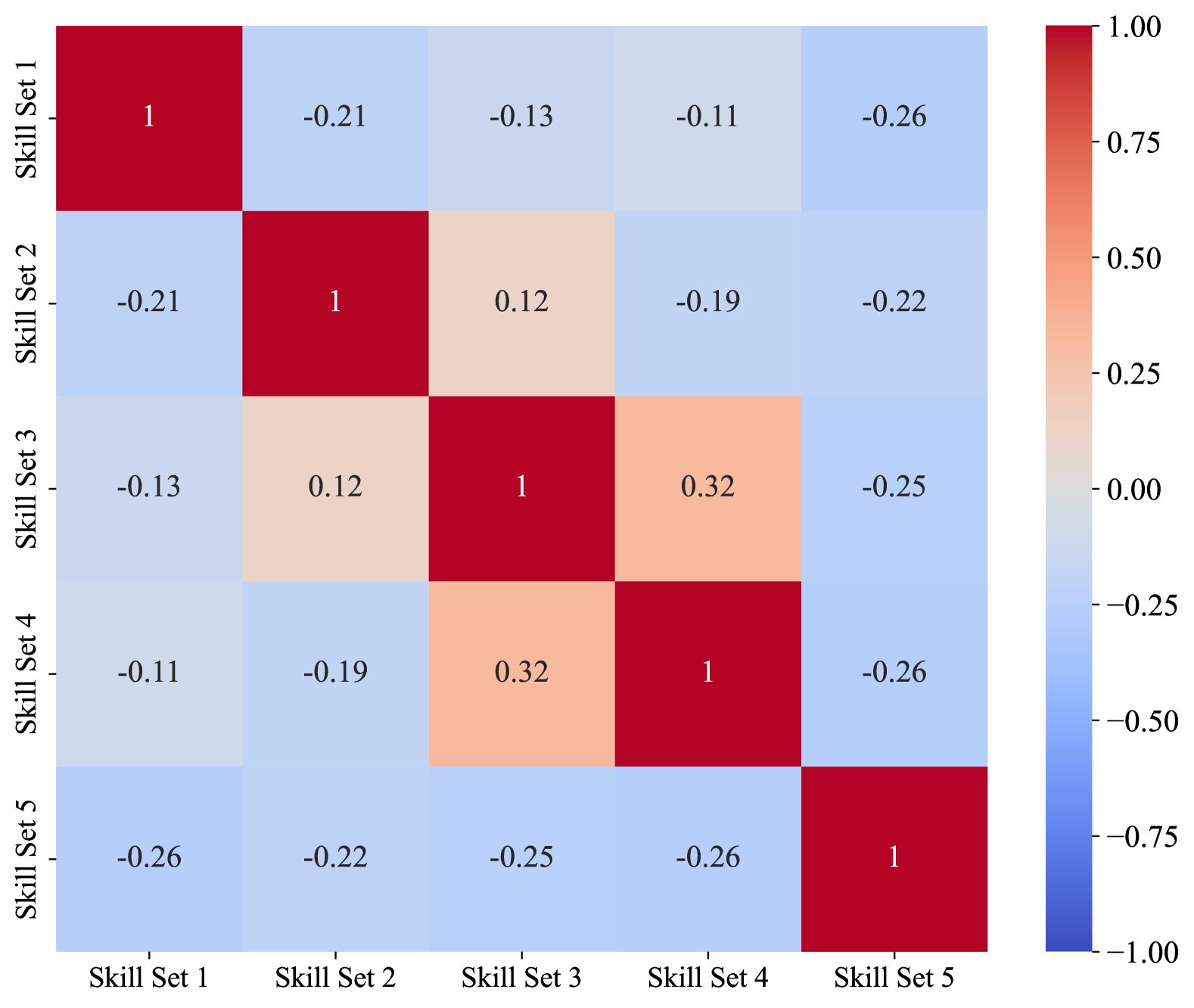
(d) Spearman correlation

Figure 10. Dataset statistics and analysis of frequent skill sets (minSup $\geq$ 0.01).

Figure 11. Reasoning process of LGDESetNet on Designer job posting.

B.2. Additional Case Study

As presented in Figure 11, we provide an additional case study using a Designer-related job posting (e.g., User-centered Design Specialist). It highlights how LGDESetNet can discern the most salary-impacting skills, noting that “User Research & Interactivity” aligns best with high similarity scores, significantly affecting salary predictions. Conversely, IT-related skills like “JavaScript” and “Database”, while potentially valuable, show low relevance to user-centered design roles and thus contribute less to salary estimations in that context. The study showcases LGDESetNet’s direct image of the whole salary reasoning process, aiding individuals in understanding skill gaps for career advancement.

Table 6. Additional performance evaluation of state-of-the-art set-based black-box models. LGDESetNet achieves comparable performance to the best-performing black-box baselines, with slight improvements. The best results are highlighted in bold.

Methods	Skill-Salary Job Postings (Sun et al., 2021)				Job Salary Benchmarking (Meng et al., 2022a)
	IT		Designer		High-tech		Finance
	RMSE ($\downarrow$)	MAE ($\downarrow$)	RMSE ($\downarrow$)	MAE ($\downarrow$)	RMSE ($\downarrow$)	MAE ($\downarrow$)	RMSE ($\downarrow$)	MAE ($\downarrow$)
DeepSets	$\text{4.271}_{\pm\text{0.020}}$	$\text{3.260}_{\pm\text{0.021}}$	$\text{3.504}_{\pm\text{0.058}}$	$\text{2.583}_{\pm\text{0.033}}$	$\text{3.361}_{\pm\text{0.064}}$	$\text{2.480}_{\pm\text{0.051}}$	$\text{3.835}_{\pm\text{0.075}}$	$\text{2.859}_{\pm\text{0.067}}$
Set Transformer	$\text{4.245}_{\pm\text{0.048}}$	$\text{3.278}_{\pm\text{0.024}}$	$\text{3.627}_{\pm\text{0.166}}$	$\text{2.702}_{\pm\text{0.181}}$	$\text{3.440}_{\pm\text{0.065}}$	$\text{2.563}_{\pm\text{0.063}}$	$\text{3.873}_{\pm\text{0.103}}$	$\text{2.883}_{\pm\text{0.091}}$
SetNorm	$\text{4.231}_{\pm\text{0.057}}$	$\text{3.262}_{\pm\text{0.023}}$	$\text{3.533}_{\pm\text{0.042}}$	$\text{2.627}_{\pm\text{0.028}}$	$\text{3.414}_{\pm\text{0.049}}$	$\text{2.538}_{\pm\text{0.028}}$	$\text{3.874}_{\pm\text{0.036}}$	$\text{2.799}_{\pm\text{0.030}}$
LGDESetNet	${\text{4.162}_{\pm\text{0.012}}}$	${\text{3.141}_{\pm\text{0.041}}}$	${\text{3.473}_{\pm\text{0.058}}}$	${\text{2.559}_{\pm\text{0.062}}}$	${\text{3.327}_{\pm\text{0.038}}}$	${\text{2.434}_{\pm\text{0.037}}}$	${\text{3.775}_{\pm\text{0.046}}}$	${\text{2.768}_{\pm\text{0.031}}}$

References

- (1)
- Ancona et al. (2017) Marco Ancona, Enea Ceolini, Cengiz Öztireli, and Markus Gross. 2017. Towards better understanding of gradient-based attribution methods for deep neural networks. arXiv preprint arXiv:1711.06104 (2017).
- Autor and Dorn (2013) David H Autor and David Dorn. 2013. The growth of low-skill service jobs and the polarization of the US labor market. American economic review 103, 5 (2013), 1553–1597.
- Burstein and Vogel (2017) Ariel Burstein and Jonathan Vogel. 2017. International trade, technology, and the skill premium. Journal of Political Economy 125, 5 (2017), 1356–1412.
- Chen et al. (2019) Chaofan Chen, Oscar Li, Daniel Tao, Alina Barnett, Cynthia Rudin, and Jonathan K Su. 2019. This looks like that: deep learning for interpretable image recognition. Advances in neural information processing systems 32 (2019).
- Chen et al. (2024) Guangyan Chen, Meiling Wang, Yi Yang, Kai Yu, Li Yuan, and Yufeng Yue. 2024. Pointgpt: Auto-regressively generative pre-training from point clouds. Advances in Neural Information Processing Systems 36 (2024).
- Cheng et al. (2016) Heng-Tze Cheng, Levent Koc, Jeremiah Harmsen, Tal Shaked, Tushar Chandra, Hrishi Aradhye, Glen Anderson, Greg Corrado, Wei Chai, Mustafa Ispir, et al. 2016. Wide & deep learning for recommender systems. In Proceedings of the 1st workshop on deep learning for recommender systems. 7–10.
- Chien et al. (2021) Eli Chien, Chao Pan, Jianhao Peng, and Olgica Milenkovic. 2021. You are allset: A multiset function framework for hypergraph neural networks. arXiv preprint arXiv:2106.13264 (2021).
- Dai and Wang (2025) Enyan Dai and Suhang Wang. 2025. Towards prototype-based self-explainable graph neural network. ACM Transactions on Knowledge Discovery from Data 19, 2 (2025), 1–20.
- Dix-Carneiro and Kovak (2015) Rafael Dix-Carneiro and Brian K Kovak. 2015. Trade liberalization and the skill premium: A local labor markets approach. American Economic Review 105, 5 (2015), 551–57.
- Fang et al. (2023) Chuyu Fang, Chuan Qin, Qi Zhang, Kaichun Yao, Jingshuai Zhang, Hengshu Zhu, Fuzhen Zhuang, and Hui Xiong. 2023. RecruitPro: A Pretrained Language Model with Skill-Aware Prompt Learning for Intelligent Recruitment. In Proceedings of the 29th ACM SIGKDD Conference on Knowledge Discovery and Data Mining. 3991–4002.
- Fauvel et al. (2023) Kevin Fauvel, Fuxing Chen, and Dario Rossi. 2023. A lightweight, efficient and explainable-by-design convolutional neural network for internet traffic classification. In Proceedings of the 29th ACM SIGKDD Conference on Knowledge Discovery and Data Mining. 4013–4023.
- Geng et al. (2020) Xinwei Geng, Longyue Wang, Xing Wang, Bing Qin, Ting Liu, and Zhaopeng Tu. 2020. How does selective mechanism improve self-attention networks? arXiv preprint arXiv:2005.00979 (2020).
- Gordon et al. (2019) Jonathan Gordon, Wessel P Bruinsma, Andrew YK Foong, James Requeima, Yann Dubois, and Richard E Turner. 2019. Convolutional conditional neural processes. arXiv preprint arXiv:1910.13556 (2019).
- Gumbel (1948) Emil Julius Gumbel. 1948. Statistical theory of extreme values and some practical applications: a series of lectures. Vol. 33. US Government Printing Office.
- Guo et al. (2017) Huifeng Guo, Ruiming Tang, Yunming Ye, Zhenguo Li, and Xiuqiang He. 2017. DeepFM: a factorization-machine based neural network for CTR prediction. In Proceedings of the 26th International Joint Conference on Artificial Intelligence. 1725–1731.
- Guo et al. (2025) Mengzhuo Guo, Qingpeng Zhang, and Daniel Dajun Zeng. 2025. An Interpretable Deep Learning-based Model for Decision-making through Piecewise Linear Approximation. ACM Transactions on Knowledge Discovery from Data (2025).
- He et al. (2024) Yi-Xiao He, Shen-Huan Lyu, and Yuan Jiang. 2024. Interpreting deep forest through feature contribution and mdi feature importance. ACM Transactions on Knowledge Discovery from Data (2024).
- Hirsch and Gilad-Bachrach (2021) Roy Hirsch and Ran Gilad-Bachrach. 2021. Trees with Attention for Set Prediction Tasks. In International Conference on Machine Learning. PMLR, 4250–4261.
- Hong et al. (2020) Dat Hong, Stephen S Baek, and Tong Wang. 2020. Interpretable sequence classification via prototype trajectory. arXiv preprint arXiv:2007.01777 (2020).
- Jiang et al. (2023) Yushan Jiang, Wenchao Yu, Dongjin Song, Lu Wang, Wei Cheng, and Haifeng Chen. 2023. FedSkill: Privacy Preserved Interpretable Skill Learning via Imitation. In Proceedings of the 29th ACM SIGKDD Conference on Knowledge Discovery and Data Mining. 1010–1019.
- Kenny et al. (2022) Eoin M Kenny, Mycal Tucker, and Julie Shah. 2022. Towards interpretable deep reinforcement learning with human-friendly prototypes. In The Eleventh International Conference on Learning Representations.
- Khuller and Saha (2009) Samir Khuller and Barna Saha. 2009. On finding dense subgraphs. In International colloquium on automata, languages, and programming. Springer, 597–608.
- Kim et al. (2022) Jinwoo Kim, Dat Nguyen, Seonwoo Min, Sungjun Cho, Moontae Lee, Honglak Lee, and Seunghoon Hong. 2022. Pure transformers are powerful graph learners. Advances in Neural Information Processing Systems 35 (2022), 14582–14595.
- Kingma and Ba (2014) Diederik P Kingma and Jimmy Ba. 2014. Adam: A method for stochastic optimization. arXiv preprint arXiv:1412.6980 (2014).
- Kolodner (1992) Janet L Kolodner. 1992. An introduction to case-based reasoning. Artificial intelligence review 6, 1 (1992), 3–34.
- Lazar (2004) Alina Lazar. 2004. Income prediction via support vector machine.. In ICMLA. 143–149.
- Lee et al. (2019) Juho Lee, Yoonho Lee, Jungtaek Kim, Adam Kosiorek, Seungjin Choi, and Yee Whye Teh. 2019. Set transformer: A framework for attention-based permutation-invariant neural networks. In International conference on machine learning. PMLR, 3744–3753.
- Lemhadri et al. (2021) Ismael Lemhadri, Feng Ruan, and Rob Tibshirani. 2021. Lassonet: Neural networks with feature sparsity. In International conference on artificial intelligence and statistics. PMLR, 10–18.
- Li et al. (2022) Junhui Li, Wensheng Gan, Yijie Gui, Yongdong Wu, and Philip S Yu. 2022. Frequent itemset mining with local differential privacy. In Proceedings of the 31st ACM International Conference on Information & Knowledge Management. 1146–1155.
- Li et al. (2018) Oscar Li, Hao Liu, Chaofan Chen, and Cynthia Rudin. 2018. Deep learning for case-based reasoning through prototypes: A neural network that explains its predictions. In Proceedings of the AAAI Conference on Artificial Intelligence.
- Li et al. (2025) Sihang Li, Yanchen Luo, An Zhang, Xiang Wang, Longfei Li, Jun Zhou, and Tat-Seng Chua. 2025. Self-attentive Rationalization for Interpretable Graph Contrastive Learning. ACM Transactions on Knowledge Discovery from Data 19, 2 (2025), 1–21.
- Li et al. (2024) Yifan Li, Shuhan Qi, Xuan Wang, Jiajia Zhang, and Lei Cui. 2024. A Novel Tree-Based Method for Interpretable Reinforcement Learning. ACM Transactions on Knowledge Discovery from Data 18, 9 (2024), 1–22.
- Lovaglio et al. (2018) Pietro Giorgio Lovaglio, Mirko Cesarini, Fabio Mercorio, and Mario Mezzanzanica. 2018. Skills in demand for ICT and statistical occupations: Evidence from web-based job vacancies. Statistical Analysis and Data Mining: The ASA Data Science Journal 11, 2 (2018), 78–91.
- Lundberg and Lee (2017) Scott M Lundberg and Su-In Lee. 2017. A unified approach to interpreting model predictions. Advances in neural information processing systems 30 (2017).
- Ma et al. (2024) Chiyu Ma, Brandon Zhao, Chaofan Chen, and Cynthia Rudin. 2024. This looks like those: Illuminating prototypical concepts using multiple visualizations. Advances in Neural Information Processing Systems 36 (2024).
- Maron et al. (2018) Haggai Maron, Heli Ben-Hamu, Nadav Shamir, and Yaron Lipman. 2018. Invariant and equivariant graph networks. arXiv preprint arXiv:1812.09902 (2018).
- Maron et al. (2020) Haggai Maron, Or Litany, Gal Chechik, and Ethan Fetaya. 2020. On learning sets of symmetric elements. In International conference on machine learning. PMLR, 6734–6744.
- Meng et al. (2022a) Qingxin Meng, Keli Xiao, Dazhong Shen, Hengshu Zhu, and Hui Xiong. 2022a. Fine-Grained Job Salary Benchmarking with a Nonparametric Dirichlet Process–Based Latent Factor Model. INFORMS Journal on Computing 34, 5 (2022), 2443–2463.
- Meng et al. (2022b) Qingxin Meng, Keli Xiao, Dazhong Shen, Hengshu Zhu, and Hui Xiong. 2022b. Job Salary Benchmarking. https://github.com/qingxin-meng/NDP-JSB.
- Meng et al. (2018) Qingxin Meng, Hengshu Zhu, Keli Xiao, and Hui Xiong. 2018. Intelligent salary benchmarking for talent recruitment: A holistic matrix factorization approach. In 2018 IEEE International Conference on Data Mining (ICDM). IEEE, 337–346.
- Miao et al. (2022) Siqi Miao, Mia Liu, and Pan Li. 2022. Interpretable and generalizable graph learning via stochastic attention mechanism. In International Conference on Machine Learning. PMLR, 15524–15543.
- Ming et al. (2019) Yao Ming, Panpan Xu, Huamin Qu, and Liu Ren. 2019. Interpretable and steerable sequence learning via prototypes. In Proceedings of the 25th ACM SIGKDD International Conference on Knowledge Discovery & Data Mining. 903–913.
- Murphy et al. (2018) Ryan L Murphy, Balasubramaniam Srinivasan, Vinayak Rao, and Bruno Ribeiro. 2018. Janossy pooling: Learning deep permutation-invariant functions for variable-size inputs. arXiv preprint arXiv:1811.01900 (2018).
- Nauta et al. (2021) Meike Nauta, Ron Van Bree, and Christin Seifert. 2021. Neural prototype trees for interpretable fine-grained image recognition. In Proceedings of the IEEE/CVF Conference on Computer Vision and Pattern Recognition. 14933–14943.
- Ng and Feldman (2014) Thomas WH Ng and Daniel C Feldman. 2014. A conservation of resources perspective on career hurdles and salary attainment. Journal of Vocational Behavior (2014).
- Pach et al. (2025) Mateusz Pach, Koryna Lewandowska, Jacek Tabor, Bartosz Michał Zieliński, and Dawid Damian Rymarczyk. 2025. LucidPPN: Unambiguous Prototypical Parts Network for User-centric Interpretable Computer Vision. In The Thirteenth International Conference on Learning Representations.
- Qi et al. (2017) Charles R Qi, Hao Su, Kaichun Mo, and Leonidas J Guibas. 2017. Pointnet: Deep learning on point sets for 3d classification and segmentation. In Proceedings of the IEEE conference on computer vision and pattern recognition. 652–660.
- Quan and Raheem (2022) Tee Zhen Quan and Mafas Raheem. 2022. Salary Prediction in Data Science Field Using Specialized Skills and Job Benefits–A Literature. Journal of Applied Technology and Innovation 6, 3 (2022), 70–74.
- Rajagopal et al. (2021) Dheeraj Rajagopal, Vidhisha Balachandran, Eduard Hovy, and Yulia Tsvetkov. 2021. Selfexplain: A self-explaining architecture for neural text classifiers. arXiv preprint arXiv:2103.12279 (2021).
- Rong et al. (2023) Yao Rong, Tobias Leemann, Thai-Trang Nguyen, Lisa Fiedler, Peizhu Qian, Vaibhav Unhelkar, Tina Seidel, Gjergji Kasneci, and Enkelejda Kasneci. 2023. Towards human-centered explainable ai: A survey of user studies for model explanations. IEEE transactions on pattern analysis and machine intelligence (2023).
- Rudin (2019) Cynthia Rudin. 2019. Stop explaining black box machine learning models for high stakes decisions and use interpretable models instead. Nature machine intelligence 1, 5 (2019), 206–215.
- Rymarczyk et al. (2021) Dawid Rymarczyk, Łukasz Struski, Jacek Tabor, and Bartosz Zieliński. 2021. Protopshare: Prototypical parts sharing for similarity discovery in interpretable image classification. In Proceedings of the 27th ACM SIGKDD Conference on Knowledge Discovery & Data Mining. 1420–1430.
- Schröder et al. (2023) Maresa Schröder, Alireza Zamanian, and Narges Ahmidi. 2023. Post-hoc Saliency Methods Fail to Capture Latent Feature Importance in Time Series Data. In ICLR 2023 Workshop on Trustworthy Machine Learning for Healthcare.
- Selvaraju et al. (2017) Ramprasaath R Selvaraju, Michael Cogswell, Abhishek Das, Ramakrishna Vedantam, Devi Parikh, and Dhruv Batra. 2017. Grad-cam: Visual explanations from deep networks via gradient-based localization. In Proceedings of the IEEE international conference on computer vision. 618–626.
- Seo et al. (2024) Sangwoo Seo, Sungwon Kim, and Chanyoung Park. 2024. Interpretable prototype-based graph information bottleneck. Advances in Neural Information Processing Systems 36 (2024).
- Sun et al. (2025) Ying Sun, Yang Ji, Hengshu Zhu, Fuzhen Zhuang, Qing He, and Hui Xiong. 2025. Market-aware Long-term Job Skill Recommendation with Explainable Deep Reinforcement Learning. ACM Transactions on Information Systems 43, 2 (2025), 1–35.
- Sun et al. (2023) Ying Sun, Fuzhen Zhuang, Hengshu Zhu, Zhang Qi, Qing He, and Hui Xiong. 2023. Job Posting Data. https://figshare.com/articles/dataset/JobPostingData/14060498/1.
- Sun et al. (2021) Ying Sun, Fuzhen Zhuang, Hengshu Zhu, Qi Zhang, Qing He, and Hui Xiong. 2021. Market-oriented job skill valuation with cooperative composition neural network. Nature communications 12, 1 (2021), 1992.
- Sundararajan et al. (2017) Mukund Sundararajan, Ankur Taly, and Qiqi Yan. 2017. Axiomatic attribution for deep networks. In International conference on machine learning. PMLR, 3319–3328.
- Ternikov (2022) Andrei Ternikov. 2022. Soft and hard skills identification: insights from IT job advertisements in the CIS region. PeerJ Computer Science 8 (2022), e946.
- Van Gog and Rummel (2010) Tamara Van Gog and Nikol Rummel. 2010. Example-based learning: Integrating cognitive and social-cognitive research perspectives. Educational psychology review 22 (2010), 155–174.
- Vaswani et al. (2017) Ashish Vaswani, Noam Shazeer, Niki Parmar, Jakob Uszkoreit, Llion Jones, Aidan N Gomez, Łukasz Kaiser, and Illia Polosukhin. 2017. Attention is all you need. Advances in neural information processing systems 30 (2017).
- Wang et al. (2021) Jiaqi Wang, Huafeng Liu, Xinyue Wang, and Liping Jing. 2021. Interpretable image recognition by constructing transparent embedding space. In Proceedings of the IEEE/CVF International Conference on Computer Vision. 895–904.
- Wu et al. (2024) Xiaoyang Wu, Li Jiang, Peng-Shuai Wang, Zhijian Liu, Xihui Liu, Yu Qiao, Wanli Ouyang, Tong He, and Hengshuang Zhao. 2024. Point Transformer V3: Simpler Faster Stronger. In Proceedings of the IEEE/CVF Conference on Computer Vision and Pattern Recognition. 4840–4851.
- Xu et al. (2018) Yifan Xu, Tianqi Fan, Mingye Xu, Long Zeng, and Yu Qiao. 2018. Spidercnn: Deep learning on point sets with parameterized convolutional filters. In Proceedings of the European conference on computer vision (ECCV). 87–102.
- Yao et al. (2024) Heming Yao, Phil Hanslovsky, Jan-Christian Huetter, Burkhard Hoeckendorf, and David Richmond. 2024. Weakly Supervised Set-Consistency Learning Improves Morphological Profiling of Single-Cell Images. In Proceedings of the IEEE/CVF Conference on Computer Vision and Pattern Recognition. 6978–6987.
- Zaheer et al. (2017) Manzil Zaheer, Satwik Kottur, Siamak Ravanbakhsh, Barnabas Poczos, Russ R Salakhutdinov, and Alexander J Smola. 2017. Deep sets. Advances in neural information processing systems 30 (2017).
- Zhang et al. (2022b) Lily Zhang, Veronica Tozzo, John Higgins, and Rajesh Ranganath. 2022b. Set norm and equivariant skip connections: Putting the deep in deep sets. In International Conference on Machine Learning. PMLR, 26559–26574.
- Zhang et al. (2022a) Zaixi Zhang, Qi Liu, Hao Wang, Chengqiang Lu, and Cheekong Lee. 2022a. Protgnn: Towards self-explaining graph neural networks. In Proceedings of the AAAI Conference on Artificial Intelligence, Vol. 36. 9127–9135.