Optimal Denoising in Score-Based Generative Models:
The Role of Data Regularity

Abstract

Score-based generative models achieve state-of-the-art sampling performance by denoising a distribution perturbed by Gaussian noise. In this paper, we focus on a single deterministic denoising step, and compare the optimal denoiser for the quadratic loss, we name “full-denoising”, to the alternative “half-denoising” introduced by Hyvärinen (2024). We show that looking at the performances in term of distance between distribution tells a more nuanced story, with different assumptions on the data leading to very different conclusions. We prove that half-denoising is better than full-denoising for regular enough densities, while full-denoising is better for singular densities such as mixtures of Dirac measures or densities supported on a low-dimensional subspace. In the latter case, we prove that full-denoising can alleviate the curse of dimensionality under a linear manifold hypothesis.

Keywords: Score-based generative modeling, Denoising, Wasserstein distance, Diffusion models

1 Introduction

Score-based generative models, or diffusion models (Sohl-Dickstein et al., 2015; Saremi and Hyvärinen, 2019; Ho et al., 2020; Song et al., 2021b), achieve state-of-the-art sampling performances by denoising a distribution perturbed by Gaussian noise. This denoising is made in several steps by removing each time a fraction of the noise, which can be seen as the discretization of a stochastic differential equation.

Here we focus on a single denoising step. This setting enables a more in-depth study, that could be generalized to multiple steps in future works, but is also relevant in practice for several reasons. Firstly, it has been used in recent work by Saremi et al. (2023), who propose an alternative formulation of diffusion models in which each step corresponds to log-concave sampling. The method first reduces the noise level by averaging multiple measurements, then tries to proximate the data distribution with a one step denoising Moreover, in the framework of stochastic localization (Montanari, 2023), one simulates a process that localizes to the distribution of interest, but as this process is simulated in finite time, the author precises that an additional step is needed, for example by taking the conditional expectation, hence denoising. This final denoising step is also present in denoising diffusion models even if not stated explicitly. Indeed, when lacking regularity assumptions on the data distribution, proofs of convergence for diffusion models fail, and to overcome this, Chen et al. (2023) use early stopping of the denoising process, as keeping a little bit of noise offsets the missing regularity. But then should we keep this extra noise or do an additional denoising step? This last step is examined here, and relies crucially on assumptions about the data distribution.

Formally, given a random variable $X\in\mathbb{R}^{d}$ with distribution $\mu_{X}$, we will define $Y=X+\varepsilon$ with $X$ and $\varepsilon$ independent and $\varepsilon\sim\mathcal{N}(0,\sigma^{2}I)$. The “optimal” denoiser, in the sense of the measurable function that minimizes $\mathbb{E}[\|X-f(Y)\|^{2}]$, is the conditional expectation $\varphi(y)=\mathbb{E}[X|Y=y]$. This value is related to the score, i.e., the gradient of the logarithm of the density $p_{Y}$ of $Y$, through Tweedie’s formula (Robbins, 1956; Miyasawa, 1961; Efron, 2011):

$$\varphi(y)=\mathbb{E}[X|Y=y]=y+\sigma^{2}\nabla\log p_{Y}(y).$$ (1)

But does it minimize the distance between the distribution $\mu_{X}$ and $\mu_{f(Y)}$ (in Wasserstein or any other distance between probability distributions)?

Of course, we want to limit the space of functions $f$ to ones we can compute. Knowing that in practice, $\nabla\log p_{Y}$ can be estimated by denoising score matching (Vincent, 2011), it is reasonable to look for an expression involving $\nabla\log p_{Y}$. In a recent paper, Hyvärinen (2024) introduces half-denoising

$$\varphi_{1/2}(y)=\frac{y+\mathbb{E}[X|Y=y]}{2}=y+\frac{\sigma^{2}}{2}\nabla\log p_{Y}(y),$$

and uses it to generate samples from $X$ with a modified Langevin algorithm. Our aim in this paper is to study in more details the performances of this half-denoising step and to compare it to full-denoising.

The general philosophy here is that the hypotheses made on the data distribution are essential to access the performances of the different denoising processes. We distinguish between two kinds of assumptions made in the literature. The first kind is to assume that the distribution of $X$ is regular enough, i.e., that it admits a density $p_{X}$ with respect to the Lebesgue measure, and that this density is smooth, for example that $x\mapsto\nabla\log p_{X}(x)$ is $L$-Lipchitz (see, e.g., Chen et al., 2023). The second kind, incompatible with the first, is to assume that the distribution as some kind of singularities, i.e., that it is concentrated on low dimensional manifolds, with pockets of mass separated by areas of low densities. This framework is known as the manifold hypothesis (see, e.g., Tenenbaum et al., 2000; Bengio et al., 2013; Fefferman et al., 2016).

Contributions.

In this work, we make the following contributions:

• We show that half-denoising is better for regular enough densities, in the sense that the distance (in MMD – maximum mean discrepancy – and in Wasserstein-$2$ distance) between the original distribution and the denoised distribution is of order $O(\sigma^{4})$, compared to $O(\sigma^{2})$ for full-denoising. We thus formalize and extend the scaling in $O(\sigma^{4})$ obtained by Hyvärinen (2024). On the contrary, full-denoising is better for singular distributions such as Dirac measures or Gaussian with small variance compared to the additional noise (section 3).

• When the variable is supported on a lower-dimensional subspace, we show that there is a trade-off between full-denoising which reduces the Wasserstein distance by ensuring that the output belongs to the subspace, and half-denoising that reduces the Wasserstein distance on the lower-dimensional subspace (assuming a regular enough density). Moreover, in the case where the subspace is of small enough dimension compared to the full space, we show that full-denoising is adaptive to this low dimensional structure and thus alleviates the curse of dimensionality as the Wasserstein distance only depends on the distance between distributions on the lower-dimensional subspace (section 4).

• We show that the denoising performance for a mixture of distributions with disjoint compact supports behaves as if we were denoising each variable independently, plus an exponentially decreasing term (section 5).

• Finally, combining these results shows that for a linear version of the manifold hypothesis, where the data distribution is supported on disjoint compact sets, each of these belonging to a (different) linear subspace of low dimension, full-denoising can alleviate the curse of dimensionality even if the support of the distribution itself spans the whole space as it adapts to the local linear structure of the distribution.

2 Notations

We introduce the following notations:

• For $\alpha\in\mathbb{R}$, we denote $\varphi_{\alpha}(y)=y+\alpha\sigma^{2}\nabla\log p_{Y}(y)$, such that $\alpha=1/2$ corresponds to half-denoising, $\alpha=1$ to full denoising (and $\alpha=0$ to no denoising at all).

• $\|\cdot\|$ the euclidean norm on $\mathbb{R}^{d}$, $B(x,r)$ the Euclidean ball of center $x$ and radius $r$.

• $\mathcal{N}(\mu,\Sigma)$ the multivariate Gaussian distribution of mean $\mu$ and covariance matrix $\Sigma$.

• For a random variable $Z\in\mathbb{R}^{n}$, we write $\mu_{Z}$ its distribution, and, when it exists, $p_{Z}$ its density with respect to the Lebesgue measure. We write $Z\sim\mu$ if $\mu_{Z}=\mu$, $Z_{1}\sim Z_{2}$ if $\mu_{Z_{1}}=\mu_{Z_{2}}$ and $Z_{1}\bot Z_{2}$ if $Z_{1}$ and $Z_{2}$ are independent. We also denote, for $\xi\in\mathbb{R}^{n}$, $\hat{p}_{Z}(\xi)=\mathbb{E}[e^{i\xi\cdot Z}]$ the characteristic function of $Z$.

• For $p\geq 1$, we define the $p$-Wasserstein distance between $Z_{1}$ and $Z_{2}$ (or $\mu_{Z_{1}}$ and $\mu_{Z_{2}}$) as

  $$W_{p}(Z_{1},Z_{2})=W_{p}(\mu_{Z_{1}},\mu_{Z_{2}})=\left(\inf_{\Gamma:\Gamma_{z_{1}}=\mu_{Z_{1}},\Gamma_{z_{2}}=\mu_{Z_{2}}}\int\|z_{1}-z_{2}\|^{p}d\Gamma(z_{1},z_{2})\right)^{1/p},$$

  where $\{\Gamma:\Gamma_{z_{1}}=\mu_{Z_{1}},\Gamma_{z_{2}}=\mu_{Z_{2}}\}$ is the set of distributions on $\mathbb{R}^{d}\times\mathbb{R}^{d}$ with marginals $\mu_{Z_{1}}$ and $\mu_{Z_{2}}$ (see, e.g., Peyré and Cuturi, 2019).

• For a reproducing kernel Hilbert space $\mathcal{H}$, with kernel $k:\mathbb{R}^{d}\times\mathbb{R}^{d}\mapsto\mathbb{R}$, we define the maximum mean discrepancy (MMD) distance (Gretton et al., 2012) between $Z_{1}$ and $Z_{2}$ (or $\mu_{Z_{1}}$ and $\mu_{Z_{2}}$) as

  $$\operatorname{MMD}_{k}(Z_{1},Z_{2})=\operatorname{MMD}_{k}(\mu_{Z_{1}},\mu_{Z_{2}})=\sup_{f\in\mathcal{H},\|f\|_{\mathcal{H}}\leq 1}\left(\mathbb{E}[f(Z_{1})]-\mathbb{E}[f(Z_{2})]\right).$$

• For $k\in\{0,1,..\}\cup\{\infty\}$, $d_{1},d_{2}$ integers, we write $\mathcal{C}^{k}(\mathbb{R}^{d_{1}},\mathbb{R}^{d_{2}})$ the functions from $\mathbb{R}^{d_{1}}$ to $\mathbb{R}^{d_{2}}$ with $k$ continuous derivatives. If $d_{2}=1$, we simply write $\mathcal{C}^{k}(\mathbb{R}^{d_{1}})$.

• For a linear operator, $A:\mathbb{R}^{d_{1}}\rightarrow\mathbb{R}^{d_{2}}$, we write $\|A\|_{\text{op}}$ the operator norm of $A$, defined by $\|A\|_{\text{op}}=\sup_{x\neq 0}\frac{\|Ax\|}{\|x\|}$.

• $\nabla$ the gradient operator, $\nabla^{2}$ the Hessian operator, $\nabla\cdot$ the divergence operator and $\Delta$ the Laplacian, that will always be taken with respect to the space variable $x\in\mathbb{R}^{d}$.

3 Half-denoising is better for regular densities

In this section, we show that half-denoising is better for regular enough densities. We start by studying Gaussian variables, for which we have closed-form expressions of the various Wasserstein distances (section 3.1). It provides insights into the behavior of the denoiser $\varphi_{\alpha}$, but will also show that the bound we prove in the following section are tight in the dependence with respect to $\sigma$. Then in section 3.2, inspired by Hyvärinen (2024), we prove a bound on the distance between the characteristic functions, $\|\hat{p}_{X}(\xi)-\hat{p}_{\varphi_{\alpha}(Y)}(\xi)\|$, that translates to bounds in MMD between the initial and the denoised distribution, under regularity assumptions on $p_{X}$. Finally in section 3.3, we prove similar bounds in Wasserstein distance, by making a link between half-denoising and one-step discretization of the diffusion ODE (Song et al., 2021b).

3.1 Gaussian variables

If $X$ is a multivariate Gaussian distribution, we can diagonalize the covariance matrix of $X$ so that up to a rotation and a translation, $X\sim\mathcal{N}(0,\operatorname{diag}(\tau_{1}^{2},\dots,\tau_{n}^{2}))$. Both the denoising and the $W_{2}$-distance can then be calculated coordinate by coordinate, so we can focus on studying Gaussian variables in $\mathbb{R}$.

If $X\sim\mathcal{N}(0,\tau^{2})$, then $Y\sim\mathcal{N}(0,\tau^{2}+\sigma^{2})$ and we can compute $\nabla\log p_{Y}(y)=\frac{-y}{\tau^{2}+\sigma^{2}}$. It leads to,

$$\varphi_{\alpha}(y)=\frac{\tau^{2}+(1-\alpha)\sigma^{2}}{\tau^{2}+\sigma^{2}}y,$$

in particular,

$$\varphi_{1}(y)=\frac{\tau^{2}}{\tau^{2}+\sigma^{2}}y,\quad\varphi_{1/2}(y)=\frac{\tau^{2}+(1/2)\sigma^{2}}{\tau^{2}+\sigma^{2}}y.$$

The denoisers are linear transformations of $Y$, and their laws are Gaussian, given by

$$\varphi_{\alpha}(Y) \sim N\left(0,\frac{(\tau^{2}+(1-\alpha)\sigma^{2})^{2}}{\tau^{2}+\sigma^{2}}\right),$$

$$\varphi_{1}(Y) \sim N\left(0,\frac{\tau^{4}}{\tau^{2}+\sigma^{2}}\right),$$

$$\varphi_{1/2}(Y) \sim\left(0,\frac{(\tau^{2}+(1/2)\sigma^{2})^{2}}{\tau^{2}+\sigma^{2}}\right).$$

For two Gaussian variables $Z_{1}\sim N(\mu_{1},\sigma_{1}^{2})$ and $Z_{2}\sim N(\mu_{2},\sigma_{2}^{2})$, the Wasserstein distance is given by (see, e.g., Peyré and Cuturi, 2019):

$$W_{2}^{2}(Z_{1},Z_{2})=(\mu_{1}-\mu_{2})^{2}+(\sigma_{1}-\sigma_{2})^{2}.$$

We can therefore compute directly the Wasserstein distances,

$$\begin{array}[]{rll}W_{2}(X,\varphi_{\alpha}(Y))&=\Big{|}\tau-\frac{\tau^{2}+(1-\alpha)\sigma^{2}}{\sqrt{\tau^{2}+\sigma^{2}}}\Big{|}&=\tau\Big{|}1-\frac{1+(1-\alpha)\left(\frac{\sigma}{\tau}\right)^{2}}{\sqrt{1+\left(\frac{\sigma}{\tau}\right)^{2}}}\Big{|},\\ W_{2}(X,\varphi_{1}(Y))&=\Big{|}\tau-\frac{\tau^{2}}{\sqrt{\tau^{2}+\sigma^{2}}}\Big{|}&=\tau\Big{|}1-\frac{1}{\sqrt{1+\left(\frac{\sigma}{\tau}\right)^{2}}}\Big{|},\\ W_{2}(X,\varphi_{1/2}(Y))&=\Big{|}\tau-\frac{\tau^{2}+\frac{1}{2}\sigma^{2}}{\sqrt{\tau^{2}+\sigma^{2}}}\Big{|}&=\tau\Big{|}1-\frac{1+\frac{1}{2}\left(\frac{\sigma}{\tau}\right)^{2}}{\sqrt{1+\left(\frac{\sigma}{\tau}\right)^{2}}}\Big{|}.\end{array}$$ (2)

In particular for $\frac{\sigma}{\tau}\ll 1$ (small noise), with an expansion in $\frac{\sigma}{\tau}$, we get that

$$W_{2}(X,\varphi_{1}(Y))\sim\frac{1}{2\tau}\sigma^{2}\text{ and }W_{2}(X,\varphi_{1/2}(Y))\sim\frac{1}{8\tau^{3}}\sigma^{4},$$

showing that half-denoising beats full-denoising in Wasserstein distance for small noises. In fact, when dividing by $\tau$ the expression in (2), we see that they only depend on the ratio $\frac{\sigma}{\tau}$. These quantities are plotted in Figure 1, where we observe the behavior in $\left(\frac{\sigma}{\tau}\right)^{2}$ for full-denoisng and in $\left(\frac{\sigma}{\tau}\right)^{4}$ for half-denoising, making half-denoising better for small noises, and we remark that it stays better up to $\frac{\sigma}{\tau}=\sqrt{8}\approx 2.83$.

Note moreover that for $\alpha=0$ (no denoising), we have

$$W_{2}(X,\varphi_{0}(Y))=W_{2}(X,Y)=\tau\left|1-\sqrt{1+\left(\frac{\sigma}{\tau}\right)^{2}}\right|\approx\frac{1}{2\tau}\sigma^{2},$$

that is, full-denoising is not better than no denoising at all!

On the contrary, for $\frac{\sigma}{\tau}\gg 1$ (large noise), we have

$$W_{2}(X,\varphi_{1}(Y))\approx\tau\text{ and }W_{2}(X,\varphi_{1/2}(Y))\approx\frac{1}{2}\sigma,$$

meaning that $W_{2}(X,\varphi_{1}(Y))\ll W_{2}(X,\varphi_{1/2}(Y))$. In fact $W_{2}(X,\varphi_{1}(Y))=0$ for a Dirac mass ($\tau=0$) whereas $W_{2}(X,\varphi_{1/2}(Y))=\frac{1}{2}\sigma$.

Finally, note that we can compute the optimal $\alpha$ for any $\tau$, as $\alpha=1+\frac{\tau^{2}}{\sigma^{2}}-\frac{\tau}{\sigma}(1+\frac{\tau^{2}}{\sigma^{2}})^{1/2}=\frac{\tau^{2}}{\sigma^{2}}(1+\frac{\sigma^{2}}{\tau^{2}}-(1+\frac{\sigma^{2}}{\tau^{2}})^{1/2})$. For $\frac{\sigma}{\tau}\ll 1$, we get $\alpha=1/2+O((\frac{\sigma}{\tau})^{2})$ and for $\frac{\sigma}{\tau}\gg 1$, $\alpha=1-\frac{\tau}{\sigma}+O((\frac{\tau}{\sigma})^{2})$. We see that the first order terms do not depend on $\tau$, and corresponds either to half-denoising or to full-denoising.

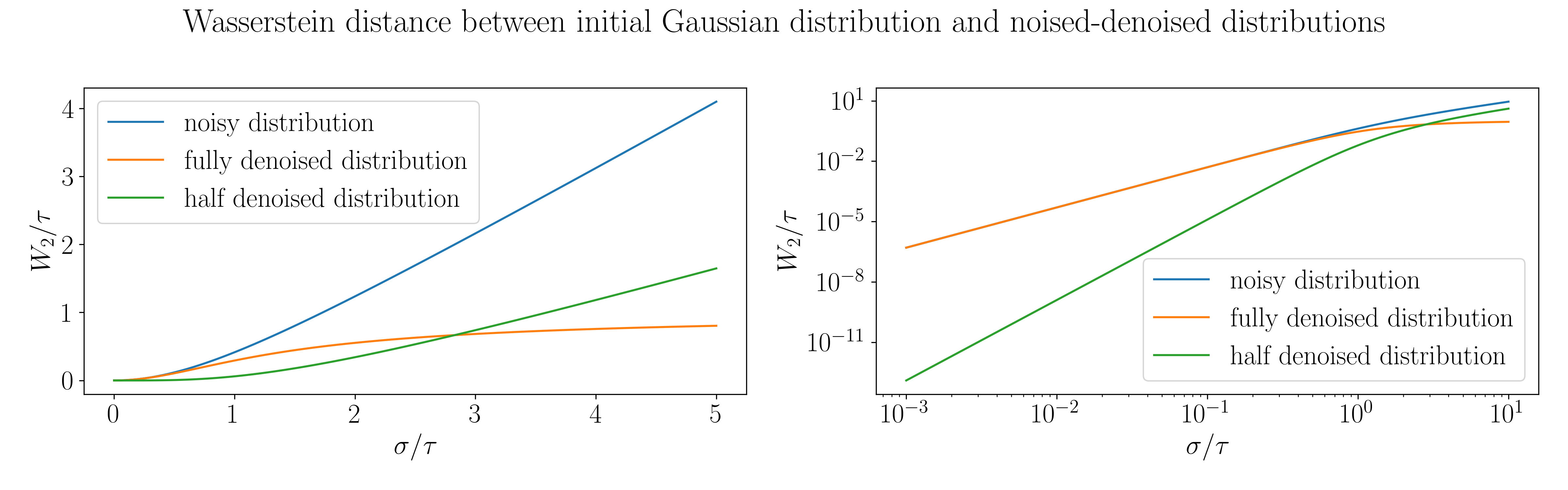
Figure 1: Wasserstein distances for Gaussian distributions at different levels of noise. Left: linear scale, right: logarithmic scale.

3.2 Half-denoising is better in MMD for variables with smooth densities

Hyvärinen (2024) shows that $\hat{p}_{\varphi_{1/2}(Y)}(\xi)=\hat{p}_{X}(\xi)+O(\sigma^{4})$. However, the proof does not keep track of the constants (in particular the dependence in $\xi$) and is incomplete due to missing assumptions. Based on the same idea, we propose a more rigorous statement and an application to MMD distances.

Proposition 1

Assume that $\mathbb{E}[\|\nabla\log p_{X}(X)\|^{2}]\leq C$. Then for all $\alpha\in\mathbb{R}$,

$$\forall\xi\in\mathbb{R}^{n},\|\hat{p}_{X}(\xi)-\hat{p}_{\varphi_{\alpha}(Y)}(\xi)\|\leq\frac{\sigma^{2}(2\alpha\sqrt{C}\|\xi\|+\|\xi\|^{2})}{2},$$

and furthermore, for $\alpha=\frac{1}{2}$,

$$\forall\xi\in\mathbb{R}^{n},\|\hat{p}_{X}(\xi)-\hat{p}_{\varphi_{1/2}(Y)}(\xi)\|\leq\frac{\sigma^{4}(C\|\xi\|^{2}+\|\xi\|^{4})}{8}.$$

(All proofs can be found in Appendix B.)

Remark: The hypothesis on the score ($\mathbb{E}[\|\nabla\log p_{X}(X)\|^{2}]\leq C$) is natural in the framework of denoising score matching, where we use a neural network to learn the score $\log p_{Y}$. Indeed, Vincent (2011) showed the learning the score with an $L_{2}$-error $\min_{\theta}\mathbb{E}[\|s_{\theta}(Y)-\nabla\log p_{Y}(Y)\|^{2}]$ is equivalent to the denoising objective $\mathbb{E}[\|X-f_{\theta}(Y)\|^{2}]$, the latter being used in practice to learn the score. Therefore, as we are learning with an $L_{2}$-error, it is natural to ask for the $L_{2}$-bound $\mathbb{E}[\|\nabla\log p_{Y}(Y)\|^{2}]\leq C$. Imposing the bound on $p_{X}$, $\mathbb{E}[\|\nabla\log p_{X}(X)\|^{2}]\leq C$, allows us to have the bound on $p_{Y}$ regardless of the level of the added noise $\sigma$ as $\mathbb{E}[\|\nabla\log p_{X}(X)\|^{2}]\leq\mathbb{E}[\|\nabla\log p_{Y}(Y)\|^{2}]$ (Lemma 10 in Appendix B). It can also be deduced from other hypotheses made in the literature. For example:

• If $X=Z+\varepsilon_{0}$ , with $Z\bot\varepsilon_{0}$ and $\varepsilon_{0}\sim\mathcal{N}(0,\tau^{2})$, and $\mathbb{E}[\|Z\|^{2}]\leq R^{2}$ (in particular if $\text{supp}(Z)\subset B(0,R)$ as assumed in Theorem 1 of Saremi et al. (2023)), we have $\mathbb{E}[\|\nabla\log p_{X}(X)\|^{2}]\leq\frac{3(2R^{2}+d\tau^{2})}{\tau^{4}}$. Indeed, with Tweedie’s formula (1),

  $$\mathbb{E}[\|\nabla\log p_{X}(X)\|^{2}] =\mathbb{E}\left[\left\|\frac{1}{\tau^{2}}(\mathbb{E}[Z|X]-X)\right\|^{2}\right]=\mathbb{E}\left[\left\|\frac{1}{\tau^{2}}(\mathbb{E}[Z|X]-Z-\varepsilon_{0})\right\|^{2}\right]$$

  $$\leq\frac{3}{\tau^{4}}(\mathbb{E}[\|\mathbb{E}[Z|X]\|^{2}]+\mathbb{E}[\|Z\|^{2}]+\mathbb{E}[\|\varepsilon_{0}\|^{2}])\quad\text{(Jensen's inequality)}$$

  $$\leq\frac{3}{\tau^{4}}(\mathbb{E}[\mathbb{E}[\|Z\|^{2}|X]]+\mathbb{E}[\|Z\|^{2}]+d\tau^{2})$$

  (Jensen’s inequality on conditional expectation)

  $$=\frac{3}{\tau^{4}}(2\mathbb{E}[\|Z\|^{2}]+d\tau^{2})\leq\frac{3}{\tau^{4}}(2R^{2}+d\tau^{2}).$$

• If $X$ is such that $x\mapsto\nabla\log p_{X}(x)$ is $L$-Lipschitz and $\mathbb{E}[\|X\|^{2}]=m_{2}<\infty$ (cf. assumptions A1 and A2 of Chen et al. (2023)), we have $\mathbb{E}[\|\nabla\log p_{X}(X)\|^{2}]\leq 2(L^{2}m_{2}+\|\nabla\log p_{X}(0)\|^{2})$.

These bounds on the characteristic functions lead to bounds in MMD distance (Gretton et al., 2012) for a translation-invariant kernel. Let $k(x,y)=\psi(x-y)$, with $\psi:\mathbb{R}^{n}\rightarrow\mathbb{R}$ a bounded, continuous positive definite function. From Bochner’s theorem, there is a finite nonnegative Borel measure $\Lambda$ on $\mathbb{R}^{n}$ such that:

$$\psi(x)=\int e^{-i\xi\cdot x}d\Lambda(\xi).$$

Then, for two random variables $X$ and $Y$, we have (Sriperumbudur et al., 2010, Corollary 4):

$$\operatorname{MMD}_{k}(X,Y)=\left(\int|\hat{p}_{X}(\xi)-\hat{p}_{Y}(\xi)|^{2}d\Lambda(\xi)\right)^{1/2}.$$

Corollary 2

Assume that, $\mathbb{E}[\|\nabla\log p_{X}(X)\|^{2}]\leq C$, and,

$$C_{2}=\int\|\xi\|^{2}d\Lambda(\xi)<\infty,\quad\quad C_{4}=\int\|\xi\|^{4}d\Lambda(\xi)<\infty,\quad\text{and }\quad C_{8}=\int\|\xi\|^{8}d\Lambda(\xi)<\infty.$$

Then, for all $\alpha\in\mathbb{R}$,

$$\operatorname{MMD}_{k}(X,\varphi_{\alpha}(Y))\leq K_{1}\sigma^{2},$$

with $K_{1}=\frac{\sqrt{4\alpha^{2}CC_{2}+C_{4}}}{\sqrt{2}}$.

Furthermore, for $\alpha=\frac{1}{2}$,

$$\operatorname{MMD}_{k}(X,\varphi_{1/2}(Y))\leq K_{2}\sigma^{4},$$

with $K_{2}=\frac{\sqrt{C^{2}C_{4}+C_{8}}}{4\sqrt{2}}.$

In particular, the first result applies for $\alpha=1$. It shows that for regular enough densities ($\mathbb{E}[\|\nabla\log p_{X}(X)\|^{2}]\leq C$), we have $\operatorname{MMD}_{k}(X,\varphi_{1/2}(Y))=O(\sigma^{4})$, whereas $\operatorname{MMD}_{k}(X,\varphi_{1}(Y))=O(\sigma^{2})$ and hence the bound on $\operatorname{MMD}_{k}(X,\varphi_{1/2}(Y))$ is negligible compare to the bound on $\operatorname{MMD}_{k}(X,\varphi_{1}(Y))$ for small $\sigma$, therefore extending the result seen above for Gaussian distributions. Moreover, the bound $\operatorname{MMD}_{k}(X,\varphi_{\alpha}(Y))=O(\sigma^{2})$ also applies for $\alpha=0$, hence as in the Gaussian case, full-denoising does not do better than no-denoising for small $\sigma$.

3.3 Half-denoising is better in Wasserstein-2 for variables with smooth densities

We now prove similar bounds in Wasserstein distance. To do so, we introduce a continuous diffusion process, adding progressively Gaussian noise to $X$ with a Brownian motion, and the diffusion ODE, that generates the same marginals with a deterministic process. This deterministic process, sometimes refer as the probability flow ODE (Song et al., 2021b), has been used as a way to have deterministic generation with diffusion models. Here, we will use the fact that half-denoising can be seen as a one step discretization of this ODE. We give a complete proof of the construction of this ODE in Appendix A. Here is a brief overview.

We define a process $X_{t}=X+B_{t}$, with $B_{t}$ a Brownian motion, such that we have $X=X_{0}$ and $Y=X_{\sigma^{2}}$. We also denote $p_{t}=p_{X_{t}}$ the density of $X_{t}$ with respect to the Lebesgue measure. $p_{t}$ verifies the Fooker-Planck equation $\partial p_{t}=\Delta p_{t}$, which can be rewritten as $\partial p_{t}=-\nabla\cdot(-p_{t}\nabla\log p_{t})$. We deduce that we can then defined the following ODE:

$$\left\{\begin{array}[]{rll}\frac{dx_{t}}{dt}&=-\frac{1}{2}\nabla\log p_{t}(x_{t})&\text{for }t>0\\ x_{t^{*}}&=X_{t^{*}}&\text{for some }t^{*}>0,\end{array}\right.$$ (3)

and that it has the same marginals as $X_{t}$: $\forall t\in[0,+\infty[,x_{t}\sim X_{t}$, and verifies, for all $t,s\geq 0$,

$$x_{t}-x_{s}=-\frac{1}{2}\int_{s}^{t}\nabla\log p_{u}(x_{u})du.$$

Note here that $\nabla\log p_{t}$ is not, in general, Lipchitz-continuous near $t=0$. That’s why we take an initial condition at $t^{*}>0$. However, we verify that the trajectory can in fact be integrated up to $t=0$ (see Appendix A for more details).

As Gentiloni-Silveri and Ocello (2025), we use the continuous time process $x_{t}$, and its one step discretization, to get natural couplings between distribution of $X$ and $\varphi_{\alpha}(Y)$ and compute Wasserstein distances. We have $X\sim x_{0}$ and $\varphi_{\alpha}(Y)\sim\hat{x}_{0}$, with $\hat{x}_{0}=x_{t}+\alpha t\nabla\log p_{t}(x_{t})$ and $t=\sigma^{2}$. This leads to the bound $W_{2}^{2}(X,\varphi_{\alpha}(Y))\leq\mathbb{E}[\|x_{0}-\hat{x}_{0}\|^{2}]$, with

$$x_{0}-\hat{x}_{0}=\frac{1}{2}\int_{0}^{t}\nabla\log p_{s}(x_{s})ds-\alpha t\nabla\log p_{t}(x_{t}).$$

To conclude, we need to be able to bound $\nabla\log p_{s}(x_{s})$ for $s\in[0,t]$, and to do that, we only need to have a bound on $\nabla\log p_{X}(X)$. Formally, we have the following result:

Proposition 3

Assume that $\mathbb{E}[\|\nabla\log p_{X}(X)\|^{2}]\leq C$. Then

$$W_{2}(X,\varphi_{\alpha}(Y))\leq\sqrt{\frac{(1+4\alpha^{2})C}{2}}\sigma^{2}.$$

For $\alpha=1$, this bound is already better (in $\sigma$) than the bound given by Proposition 2 of Saremi et al. (2023) which is $W_{2}(X,\varphi_{1}(Y))=O(\sigma)$. Moreover this bound is tight (in $\sigma$) as for a Gaussian variable with variance $\tau^{2}$, we have $W_{2}(X,\varphi_{1}(Y))\sim\frac{1}{2\tau}\sigma^{2}$ for small enough $\sigma$. Note that if we remove the assumption (i.e., $C=+\infty$), then we fall back on the bound by Saremi et al. (2023) (take for example $X$ a Dirac mass, for which we have seen that $W_{2}(X,\varphi_{1/2}(Y))=\frac{1}{2}\sigma$).

But for $\alpha=\frac{1}{2}$ we can hope to have a better bound, in $\sigma^{4}$, as it was the case with the MMD distance. Indeed, we have:

$$x_{0}-\hat{x}_{0} =\frac{1}{2}\int_{0}^{t}\nabla\log p_{s}(x_{s})ds-\frac{1}{2}t\nabla\log p_{t}(x_{t})$$

$$=\frac{1}{2}\int_{0}^{t}\left(\nabla\log p_{s}(x_{s})-\nabla\log p_{t}(x_{t})\right)ds$$

$$=\frac{1}{2}\int_{0}^{t}\int_{s}^{t}\frac{d}{du}\left(\nabla\log p_{u}(x_{u})\right)duds.$$

If we can control $\mathbb{E}[\|\frac{d}{d\mathcolor{red}{t}}\nabla\log p_{\mathcolor{red}{t}}(x_{\mathcolor{red}{t}})\|^{2}]\leq C$, we will get $\mathbb{E}[\|x_{0}-x_{t}\|^{2}]=O(t^{4})$ hence $W_{2}(X,\varphi_{1/2}(Y))=O(\sigma^{4})$. Formally, we need the following lemma:

Lemma 4

Assume that the variable $X$ of density $p_{X}$ satisfies:

• $\log p_{X}\in\mathcal{C}^{3}(\mathbb{R}^{d})$.

• $C_{1}=\mathbb{E}[\|\nabla\log p_{X}(X)\|^{6}]<\infty$.

• $C_{2}=\mathbb{E}[\|\nabla^{2}\log p_{X}(X)\|_{\textnormal{op}}^{3}]<\infty$, where $\|A\|_{\textnormal{op}}$ is defined for any matrix $A$ as $\|A\|_{\textnormal{op}}=\sup_{x\neq 0}\frac{\|Ax\|}{\|x\|}$.

• $C_{3}=\mathbb{E}[\|\nabla\Delta\log p_{X}(X)\|^{2}]<\infty$.

Then,

$$\mathbb{E}\left[\left\|\frac{d}{dt}\nabla\log p_{t}(x_{t})\right\|^{2}\right]\leq C,$$

with $C=\frac{9}{4}(4C_{1}+(2d^{2}+5)C_{1}^{1/3}C_{2}^{2/3}+C_{3})$.

Using this lemma, we have the following proposition:

Proposition 5

Under the assumptions of Lemma 4, we have

$$W_{2}(X,\varphi_{1/2}(Y))\leq K\sigma^{4}.$$

with $K=\frac{\sqrt{3}}{4}\sqrt{4C_{1}+(2d^{2}+5)C_{1}^{1/3}C_{2}^{2/3}+C_{3}}$.

Remarks:

• In Appendix C, we show that if $X=Z+\varepsilon_{0}$ , with $\mathbb{E}[\|Z\|^{6}]<\infty$, $Z\bot\varepsilon_{0}$ and $\varepsilon_{0}\sim\mathcal{N}(0,\tau^{2})$, then $X$ verifies the assumptions of Lemma 4. In particular, it applies to the case of $\text{supp}(Z)\subset B(0,R)$, assumed in Theorem 1 of Saremi et al. (2023), as then $\mathbb{E}[\|Z\|^{6}]\leq R^{6}$. It also proves that a mixture of Gaussian distributions verifies the hypothesis (take $\tau$ the smallest eigenvalue of all the covariances matrices of the Gaussian distributions in the mixture).

• The assumptions of Lemma 4 and Proposition 5 control the regularity of the density $p_{X}$. The fact that we need to bound derivative up to order 3 comes directly from the Fokker-Planck equation $\partial_{t}p_{t}=\Delta p_{t}$, which heuristically can be interpreted as “one derivative in $t$ equals two derivatives in $x$”, hence to control $\frac{d}{dt}\nabla\log p_{t}(x_{t})$, we need to control derivatives in $x$ up to order 3.

• The control of the Hessian $\|\nabla^{2}\log p_{X}(x)\|_{\textnormal{op}}$ corresponds to controlling the Lipchitz constant of the function $x\mapsto\nabla\log p_{X}(x)$ and is an assumption usually done in the literature (see, e.g., Chen et al., 2023, assumption A1). Having an uniform bound is a strong assumption, and in particular it implies that the distribution has full support on $\mathbb{R}^{d}$. But here we only need to control this quantity in expectation under the law of $X$. As a consequence, this result can apply to distribution such that $x\mapsto\nabla\log p_{X}(x)$ is not globally Lipchitz-continuous, and moreover it does not even have to be defined everywhere. Take for example,

  $$p_{X}(x)=\left\{\begin{array}[]{cl}\frac{1}{Z}e^{-\frac{1}{1-x^{2}}}&\text{if }|x|\leq 1\\ 0&\text{otherwise},\end{array}\right.$$

  where $Z$ is a normalizing constant (Fig. 2). Then $\log p_{X}(x)=-\frac{1}{1-x^{2}}$ is only defined on the interval $(-1,1)$ and we have:

  $$\nabla\log p_{X}(x) =-\frac{2x}{\left(1-x^{2}\right)^{2}},$$

  $$\nabla^{2}\log p_{X}(x) =-\frac{2\left(3x^{2}+1\right)}{\left(1-x^{2}\right)^{3}},$$

  $$\nabla\Delta\log p_{X}(x) =-\frac{24x\left(x^{2}+1\right)}{\left(1-x^{2}\right)^{4}},$$

  with none of theses quantities being bounded on $(-1,1)$. However, our assumptions only require the bounds in expectation, and as the density $p_{X}$ decreases exponentially fast when $|x|\rightarrow 1$, overcoming the polynomial growth of the derivatives, all three constants $C_{1}$, $C_{2}$ and $C_{3}$ are finite.

  Note that as Propositions 3 and 5 can be applied to distributions with compact support, they can be combined with Proposition 7 of section 5.

• The assumptions are not verified for a very singular distribution, e.g., a Dirac $\mu_{X}=\delta_{0}$, for which $\log p_{X}$ is not even defined. In this case, we have $x_{t}\sim\mathcal{N}(0,tI)$ hence $\log p_{t}(x)=-\frac{\|x\|^{2}}{2t}$, $\nabla\log p_{t}(x)=-\frac{x}{t}$ and $\mathbb{E}[\|\nabla\log p_{t}(X)\|^{2}_{\text{op}}]=\frac{d}{t}$, which is not bounded, and not integrable near $0$. The result of Proposition 5 don’t apply, and indeed we have (cf. section 3.1) $W_{2}(X,\varphi_{1/2}(Y))=\frac{\sigma}{2}$ whereas $W_{2}(X,\varphi_{1}(Y))=0$.

• All results from this subsection can be extended to Wasserstein-$p$ distance for any $p\geq 1$ (see Appendix D).

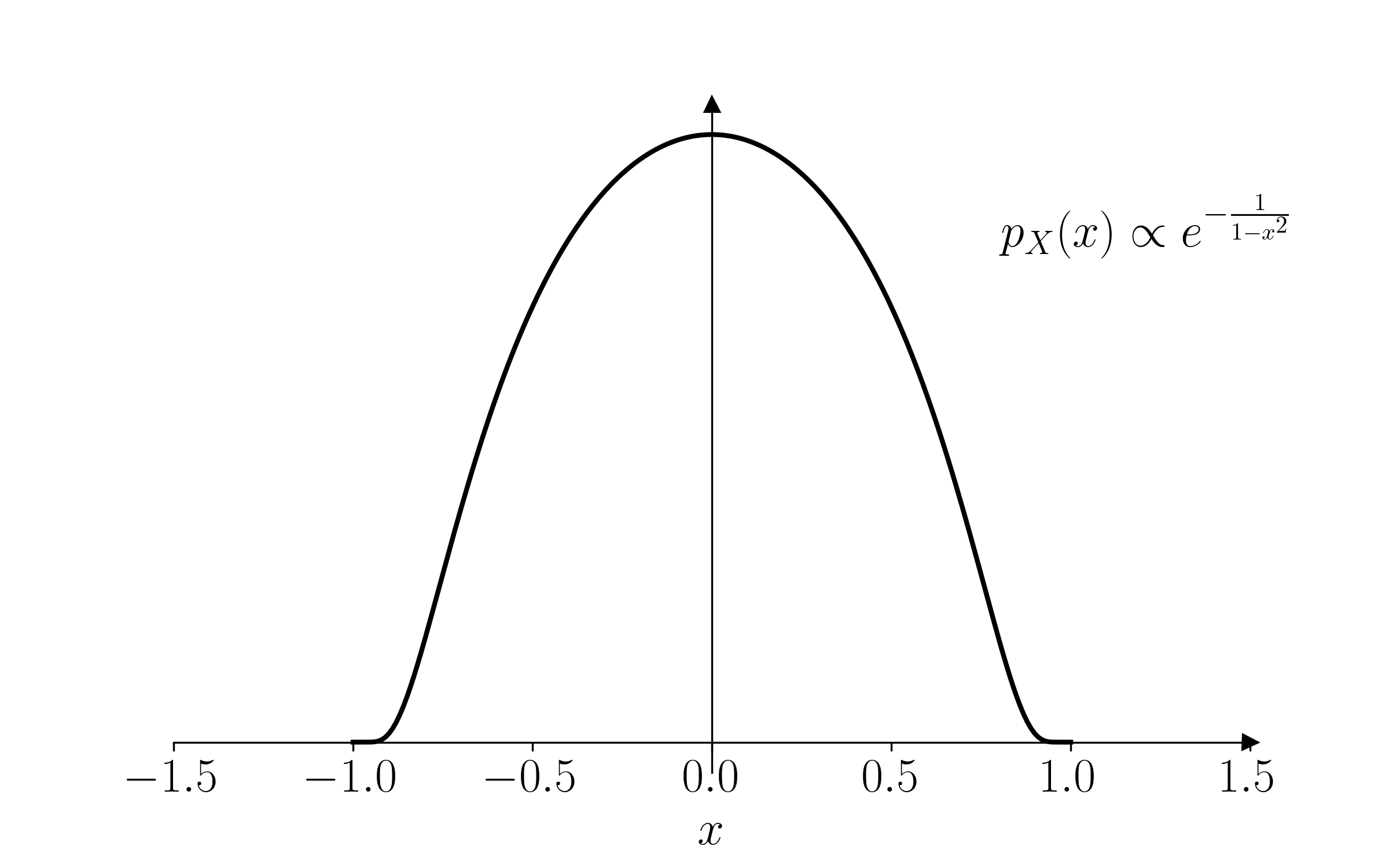
Figure 2: Example of a smooth density with a compact support.

4 Variable with support on a subspace: balancing between the impacts of singularity and regularity of the distribution

In many practical applications, the data distribution is supported on a lower dimensional manifold, a case known as the manifold hypothesis (see, e.g., Tenenbaum et al., 2000; Bengio et al., 2013; Fefferman et al., 2016). Locally, this manifold will look like a linear space, therefore, we take a look at the idealized case when the variable is supported on a linear lower-dimensional subspace.

Proposition 6

Assume that $X$ is supported on a linear subspace $H$ of dimension $m$, with $m\leq d$. Write $X_{1}=p_{H}(X)$, with $p_{H}$ the orthogonal projection on $H$, and $Y_{1}=X_{1}+\varepsilon_{1}$ with $\varepsilon_{1}\sim\mathcal{N}(0,\sigma^{2}I)$. Then:

$$W_{2}^{2}(X,\varphi_{\alpha}(Y))=W_{2}^{2}(X_{1},\varphi_{\alpha}(Y_{1}))+(d-m)(1-\alpha)^{2}\sigma^{2}.$$

We can interpret this result as trade off between $\alpha=1$ (full-denoising) which cancels the second term, as it ensures that $\varphi_{\alpha}(Y)$ belongs to the subspace $H$, and $\alpha=1/2$ (half-denoising) that will reduce the first term if $p_{X_{1}}$ is regular enough to apply the results of the previous section.

We also see that full-denoising is adaptive to the low dimensional structure of the data, as the Wasserstein distance only depends on the distance between distributions on the lower-dimensional subspace. Therefore, in the case where $m\ll d$, it alleviates the curse of dimensionality.

5 Mixtures of distributions with disjoint compact supports behave like independent variables

In the case of the manifold hypothesis, it is also common to suppose that the distribution is made of small pockets with high density of probability, representing different classes of objects, separated by regions of low density. We model this case be saying that the distribution of $X$ is a mixture of distributions with disjoint compact supports. In this case, we show that the denoising performance for a mixture of distributions with disjoint compact supports behaves as if we were denoising each variable independently, plus an exponentially decreasing term.

More formally, let $X\sim\mu_{X}=\sum_{i=1}^{N}\pi_{i}\mu_{i}$ (with $\sum_{i=1}^{N}\pi_{i}=1,\pi_{i}\geq 0$ ) a mixture of distribution $\mu_{i}$ with compact support $S_{i}$ such that $D=\min_{i\neq j}d(S_{i},S_{j})>0$ (with $d(S_{i},S_{j})=\min_{x_{i}\in S_{i},x_{j}\in S_{j}}\|x_{i}-x_{j}\|$). We denote $Y=X+\varepsilon$ with $X\bot\varepsilon$ and $\varepsilon\sim\mathcal{N}(0,\sigma^{2}I)$, for $\sigma>0$. For $\alpha\in\mathbb{R}$, we denote $\varphi_{\alpha}(y)=y+\alpha\sigma^{2}\nabla\log p_{Y}(y)$, $\nu$ the law of $Y$ and $\mu_{\alpha}$ the law of $\varphi_{\alpha}(Y)$. Similarly, for $X_{i}\sim\mu_{i}$, and $Y_{i}=X_{i}+\varepsilon$ with $X_{i}\bot\varepsilon$ and $\varepsilon\sim\mathcal{N}(0,\sigma^{2}I)$, we denote $\varphi_{i,\alpha}(y)=y+\alpha\sigma^{2}\nabla\log p_{Y_{i}}(y)$, $\nu_{i}$ the law of $Y_{i}$ and $\mu_{i,\alpha}$ the law of $\varphi_{i,\alpha}(Y_{i})$. We have the following proposition:

Proposition 7

We have, under the above assumptions,

$$W_{2}^{2}(\mu_{X},\mu_{\alpha})\leq 2\sum_{i}\pi_{i}W_{2}^{2}(\mu_{i},\mu_{i,\alpha})+O\left(\frac{1}{\sigma^{\max(d-2,8)}}\exp\left(-\frac{K}{\sigma^{2}}\right)\right),$$

where $K$ is a constant that depends only on D.

The $O$ hides a constant depending on $\alpha$, $d$, $N$ and $R$ such that $\text{supp}(X)\subset B(0,R)$ (see the proof in Appendix B for more details).

In the case where the $\mu_{i}$’s are Dirac masses, and for $\alpha=1$, we have $W_{2}^{2}(\mu_{i},\mu_{i,\alpha})=0$, hence

$$W_{2}^{2}(\mu_{X},\mu_{\alpha})=O\left(\frac{1}{\sigma^{\max(d-2,8)}}\exp\left(-\frac{K}{\sigma^{2}}\right)\right),$$

which is way better than polynomial rates in $\sigma$ seen above.

6 Consequences

Linear manifold hypothesis.

We can combine Propositions 6 and 7 to tackle what we call the linear manifold hypothesis. We defined the linear manifold hypothesis as a simplified version of the manifold hypothesis, where the data distribution is supported on disjoint compact sets, each of these belonging to a (different) linear subspace of low dimension, as illustrated in Figure 3. Then applying Proposition 7 allows to bound the Wasserstein distance between the original distribution and the fully denoised distribution by the sum of the Wasserstein distances between the distributions on each compact sets (plus on exponentially decreasing term). As each compact set belongs to a low-dimensional subspace, we can apply Proposition 6, which tells that for full-denoising, the Wasserstein distance depends only on the distribution on the sub-space. In this case, we see that full-denoising can alleviate the curse of dimensionality even if the support of the mixture distribution itself spans the whole space as it adapts to the local linear structure of the distribution. More generally, understanding the performances of score-based generative models for data distribution supported on a low dimensional manifold is an active area of research (see, e.g., Tang and Yang, 2024; Azangulov et al., 2024), and we hope that our result could be generalized with good assumption on the regularity/smoothness of the manifold.

(a)

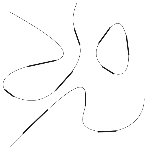
(b)

Figure 3: Illustration of the linear manifold hypothesis (a – thick line), and the manifold hypothesis (b – fine line).

Denoising diffusion models.

We will briefly discuss the first insights that our results on one step denoising give about multi-step diffusion models, leaving a further analysis for future work. We will focus on diffusion models with a deterministic denoising process, such as the probability flow ODE by Song et al. (2021b) and DDIM by Song et al. (2021a). In both cases, for a number of steps $T$, we have variable $X_{0},\dots,X_{T}$ such that $X_{t}\sim X+\mathcal{N}(0,\sigma_{t}^{2})$ with $0=\sigma_{0}<\sigma_{1}<\cdots<\sigma_{T}$, that we approximate by first sampling $\hat{X}_{T}\sim\mathcal{N}(0,\sigma_{t}^{2})\approx X_{T}$, then proceeding backward with:

$$\hat{X}_{t}=\hat{X}_{t+1}+\alpha_{t}(\sigma_{t+1}^{2}-\sigma_{t}^{2})\nabla\log p_{\sigma_{t+1}^{2}}(\hat{X}_{t+1}),$$

with $\alpha_{t}=\frac{1}{2}$ for the probability flow ODE and $\alpha_{t}=\frac{\sigma_{t+1}}{\sigma_{t}+\sigma_{t+1}}$ for DDIM. For the probability flow ODE, $\alpha_{t}=\frac{1}{2}$ corresponds simply to the Euler discretization of (3) with a varying step size $h_{t}=\sigma_{t+1}^{2}-\sigma_{t}^{2}$. For DDIM, $\alpha_{t}$ depends on $t$. At the first steps ($t$ close to $T$) of the denoising process, if we assume that $\sigma_{t+1}=\sigma_{t}+\Delta t$ with $\Delta t\ll\sigma_{t}$, then we have $\alpha_{t}\approx\frac{1}{2}$, but for the last step of the denoising process, we have $\alpha_{0}=\frac{\sigma_{1}}{0+\sigma_{1}}=1$, which corresponds to full-denoising, and intermediate steps are in between half and full-denoising. Note that this is not surprising, as DDIM is exact if the data distribution is a Dirac (Nakkiran et al., 2024), a distribution for which full-denoising is also exact.

With our previous result, we see that the choice of $\alpha_{t}$ made for the probability flow ODE is more adapted to regular densities, while the one of DDIM is more adapted to distributions with low-dimensional structures. More generally, it highlights the fact that $\alpha_{t}$ should be chosen considering the properties of the data distribution, and we believe it would be interesting to see if it could be fine-tuned in a data dependent way.

7 Conclusion

We have shown that half-denoising is better than full-denoising for regular enough densities, while full-denoising is better for singular densities such as mixtures of Dirac measures or Gaussian with small variance compare to the additional noise. Moreover, the performances of the denoisers can be further accessed with additional assumptions on the data distributions, that occurs naturally in real world data, for example with images under the manifold hypothesis.

When the variable is supported on a lower-dimensional subspace, we have shown that there is a trade off between full-denoising which reduces the Wasserstein distance by ensuring that the output belongs to the subspace, and half-denoising that reduces the Wasserstein distance on the lower-dimensional subspace assuming a regular enough density. In the case where the subspace is of small enough dimension compared to the full space, full-denoising alleviates the curse of dimensionality as the Wasserstein distance only depends on the distance between distributions on the lower-dimensional subspace. Moreover, we have shown that the denoising performance for a mixture of distributions with disjoint compact supports behaves as if we were denoising each variable independently, plus an exponentially decreasing term. This led to a case we called linear manifold hypothesis, where the data distribution is supported on disjoint compact sets, each of these belonging to a (different) linear subspace of low dimension, and for which full-denoising can alleviate the curse of dimensionality even if the support of the distribution itself spans the whole space, as it adapts to the local linear structure of the distribution.

They are several avenues to be explored to extend this work. We could try to extend our results for the linear manifold to a more general low-dimensional manifold, providing good assumptions on the regularity/smoothness of the manifold. It would also by interesting to understand what happens in the case where multiples denoising steps are repeated, as it is usually done with diffusion models and compare to existing theoretical result on the performances of the models (see, e.g., Bortoli, 2022; Chen et al., 2023; Gentiloni-Silveri and Ocello, 2025). We hope that the techniques developed here could lead to a better understanding of the Wasserstein error of diffusion models, both for deterministic sampling (discretization of the diffusion ODE (3)) and stochastic sampling (discretization of a reverse time SDE). To do so, one should also take into account the error at initialization (approximating the noised distribution by a Gaussian), the impact of the (possibly varying) step size, of the noise schedule (Strasman et al., 2025) and the error in learning the score. For the latter, it would be interesting to include results on the ability of neural networks to learn the score for distributions supported on a lower-dimensional manifold, as done by Tang and Yang (2024) and by Azangulov et al. (2024).

Acknowledgments and Disclosure of Funding

We thank Saeed Saremi for insightful discussions related to this work. This work has received support from the French government, managed by the National Research Agency, under the France 2030 program with the reference “PR[AI]RIE-PSAI” (ANR-23-IACL-0008).

Appendix A Fokker-Planck equation and the diffusion ODE

In this section, we give a short proof of the Fokker-Planck equation, and use it to define the ODE (3) presented in section 3.3. There are many references about Fokker-Planck equations (see, e.g., Risken, 1996; Bogachev et al., 2015), but here we try to give a proof as simple and self-contain as possible. For general results on SDEs, we refer the reader to Le Gall (2016). We will always assume, but note explicitly write, that we have a probability space, a filtration and a Brownian motion such that all randoms variables are well defined.

We study the process $X_{t}=X+B_{t}$, in particular, $X_{t}=X+tZ$ with $X\bot Z$, $Z\sim\mathcal{N}(0,I)$. From that we deduce that $X_{t}$ admit a density $p_{t}$ with respect to the Lebesgue measure that verifies, for $t>0$,

$$p_{t}(x)=\int\frac{\exp\left(-\|x-u\|^{2}/2t\right)}{(2\pi t)^{d/2}}d\mu_{X}(u)>0,$$

and that $(t,x)\mapsto p_{t}(x)$ is $\mathcal{C}^{\infty}$.

The evolution of the marginal $p_{t}$ is dictated by a partial differential equation, the Fokker-Planck equation.

Proposition 8 (Fokker-Planck equation)

Let $f\in\mathcal{C}^{1}(\mathbb{R}\times\mathbb{R}^{d},\mathbb{R}^{d})$, $g\in\mathcal{C}^{0}(\mathbb{R},\mathbb{R})$, and $p_{t}$ the density of a process $X_{t}$ that verifies the following SDE

$$dX_{t}=f(t,X_{t})dt+g(t)dB_{t},$$ (4)

and assume that $(t,x)\mapsto p_{t}(x)$ is $\mathcal{C}^{2}$ on $\mathbb{R}_{+}^{*}\times\mathbb{R}^{d}$. Then for all $t>0$, we have

$$\partial_{t}p_{t}=-\nabla\cdot(fp_{t})+\frac{1}{2}g^{2}\Delta p_{t}.$$

Proof  Let $\varphi\in\mathcal{C}^{\infty}(\mathbb{R}^{d},\mathbb{R})$ with compact support. Then for $t>0$,

$$\int\varphi(x)\partial_{t}p_{t}(x)dx =\int\varphi(x)\lim_{h\rightarrow 0}\frac{p_{t+h}(x)-p_{t}(x)}{h}dx$$

$$=\lim_{h\rightarrow 0}\frac{1}{h}\left(\int\varphi(x)p_{t+h}(x)dx-\int\varphi(x)p_{t}(x)dx\right)$$

$$=\lim_{h\rightarrow 0}\frac{1}{h}\mathbb{E}[\varphi(X_{t+h})-\varphi(X_{t})].$$

By Itō’s formula,

$$\varphi(X_{t+h})-\varphi(X_{t}) =\int_{t}^{t+h}\nabla\varphi(X_{s})\cdot dX_{s}+\frac{1}{2}\int_{t}^{t+h}\Delta\varphi(X_{s})d\langle X,X\rangle_{s}$$

$$=\int_{t}^{t+h}\nabla\varphi(X_{s})\cdot f(s,X_{s})ds+\int_{t}^{t+h}g(s)\nabla\varphi(X_{s})\cdot dB_{s}$$

$$\quad+\frac{1}{2}\int_{t}^{t+h}\Delta\varphi(X_{s})g(s)^{2}ds.$$

Taking the expectation, we get that,

$$\mathbb{E}[\varphi(X_{t+h})-\varphi(X_{t})]=\int_{t}^{t+h}\mathbb{E}[\nabla\varphi(X_{s})\cdot f(s,X_{s})]ds+0+\frac{1}{2}\int_{t}^{t+h}E[\Delta\varphi(X_{s})]g(s)^{2}ds.$$

As $\varphi$ has compact support, integration by part gives:

$$\mathbb{E}[\nabla\varphi(X_{s})\cdot f(s,X_{s})]=\int\nabla\varphi(x)\cdot f(s,x)p_{s}(x)dx=-\int\varphi(x)\nabla\cdot(f(s,x)p_{s}(x))dx,$$

and

$$E[\Delta\varphi(X_{s})]=\int\Delta\varphi(x)p_{s}(x)dx=\int\varphi(x)\Delta p_{s}(x)dx.$$

It follows that,

$$\int \varphi(x)\partial_{t}p_{t}(x)dx$$

$$=\lim_{h\rightarrow 0}\frac{1}{h}\left(-\int_{t}^{t+h}\int\varphi(x)\nabla\cdot(f(s,x)p_{s}(x))dxds+\frac{1}{2}\int_{t}^{t+h}\int\varphi(x)g(s)^{2}\Delta p_{s}(x)dxds\right)$$

$$=-\int\varphi(x)\nabla\cdot(f(t,x)p_{t}(x))dx\frac{1}{2}\int\varphi(x)g(t)^{2}\Delta p_{t}(x)dx,$$

as both integrands are continuous with respect to time, and we can rewrite,

$$\int\varphi(x)\left(\partial_{t}p_{t}(x)+\nabla\cdot(f(t,x)p_{t}(x))-\frac{1}{2}g(t)^{2}\Delta p_{t}(x)\right)dx=0,$$

for all $\varphi\in\mathcal{C}^{\infty}(\mathbb{R}^{d},R)$ with compact support. It follows that for all $t>0$, almost surely in $x$,

$$\partial_{t}p_{t}(x)=-\nabla\cdot(f(t,x)p_{t}(x))+\frac{1}{2}g(t)^{2}\Delta p_{t}(x),$$

which gives the desired result as these quantities are continuous in $x$.  

For the process $X_{t}=X+B_{t}$, we have $dX_{t}=dB_{t}$, which is (4) with $f=0$ and $g=1$. The Fokker-Planck equation is therefore

$$\partial_{t}p_{t}=\frac{1}{2}\Delta p_{t}.$$

As $\Delta p_{t}=\nabla\cdot\nabla p_{t}=\nabla\cdot\frac{p_{t}}{p_{t}}\nabla p_{t}=\nabla\cdot p_{t}\nabla\log p_{t}$, the equation can be rewritten as

$$\partial_{t}p_{t}=-\nabla\cdot\left(-\frac{1}{2}\nabla\log p_{t}\right)p_{t},$$

which correspond to the Fokker-Planck equation with drift term $f(t,x)=-\frac{1}{2}\nabla\log p_{t}(x)$. This allows use to define the diffusion ODE, used in section 3.3.

Proposition 9

Let $t^{*}>0$. We can define a process $(x_{t})_{t\geq 0}$ by

$$\left\{\begin{array}[]{rll}\frac{dx_{t}}{dt}&=-\frac{1}{2}\nabla\log p_{t}(x_{t})&\text{for }t>0\\ x_{t^{*}}&=X_{t^{*}}.\end{array}\right.$$ (3)

This process has the same marginals as $X_{t}$: $\forall t\in[0,+\infty[,x_{t}\sim X_{t}$, and verifies, for all $t,s\geq 0$,

$$x_{t}-x_{s}=-\frac{1}{2}\int_{s}^{t}\nabla\log p_{u}(x_{u})du.$$

Proof  We know that for $t>0$, $(t,x)\mapsto p_{t}(x)$ is $\mathcal{C}^{\infty}$. In particular, the ODE defined by (3) can be solved for all time $t>0$, and we have for $s,t>0$:

$$x_{t}-x_{s}=-\frac{1}{2}\int_{s}^{t}\nabla\log p_{u}(x_{u})du.$$ (5)

For now, we will write $\tilde{p}_{t}$ the density of the marginal of $x_{t}$. As $x_{t}$ is defined as the solution of an ODE, we introduce the resolvent $R(s,t,x)$ that gives the solution at time $t$ of the ODE

$$y^{\prime}=-\frac{1}{2}\nabla\log p_{t}(y),$$

with initial condition $x$ at time $s$. $R$ is invertible and verifies $R(s,t,x)^{-1}=R(t,s,x)$. Moreover, as $(t,x)\mapsto\nabla\log p_{t}(x)$ is $C^{\infty}$, $R$ is also $\mathcal{C}^{\infty}$ (see, e.g. Paulin, 2009, Théorème 7.21).

By construction, $x_{t}=R(t^{*},t,X_{t^{*}})$, leading to:

$$\tilde{p}_{t}(x)=|\det\nabla R(t,t^{*},x)|p_{t^{*}}(R(t,t^{*},x)),$$

in particular, $(t,x)\mapsto\tilde{p}_{t}(x)$ is $\mathcal{C}^{\infty}$ on $\mathbb{R}_{+}^{*}\times\mathbb{R}^{d}$. We can apply proposition 8, to get that

$$\partial_{t}\tilde{p}_{t}=\nabla\cdot\left(-\frac{1}{2}\nabla\log p_{t}\right)=-\frac{1}{2}\Delta\log p_{t}=\partial_{t}p_{t},$$

and as $\tilde{p}_{t^{*}}=p_{t^{*}}$, it leads to $\tilde{p}_{t}=p_{t}$ for all $t>0$.

We finally need to verify that we can extend (5) up to time $s=0$, i.e., that the trajectories can be integrated up to time $t=0$. For $t>0$, Tweedie’s formula (1) gives:

$$\nabla\log p_{t}(x)=\frac{1}{t}(x-\mathbb{E}[X|X_{t}=x]).$$

In particular, as $x_{t}$ and $X_{t}$ have the same distribution,

$$\mathbb{E}[\|\nabla\log p_{t}(x_{t})\|]=\frac{1}{t}\mathbb{E}[\|X_{t}-\mathbb{E}[X|X_{t}]\|]=\frac{1}{t}\mathbb{E}[\|\mathbb{E}[X_{t}-X|X_{t}]\|].$$

Jensen’s inequality gives

$$\mathbb{E}[\|\mathbb{E}[X_{t}-X|X_{t}]\|] \leq\mathbb{E}[\mathbb{E}[\|X_{t}-X\||X_{t}]]=\mathbb{E}[\|X_{t}-X\|]$$

$$\leq\sqrt{\mathbb{E}[\|X-X_{t}\|^{2}]}=\sqrt{\mathbb{E}[\|B_{t}\|^{2}]}=\sqrt{td},$$

therefore,

$$\mathbb{E}[\|\nabla\log p_{t}(x_{t})\|]\leq\sqrt{\frac{d}{t}},$$

which is integrable near $0$. We get that

$$\mathbb{E}\left[\int_{0}^{t}\|\nabla\log p_{u}(x_{u})\|du\right]<\infty,$$

hence

$$\int_{0}^{t}\|\nabla\log p_{u}(x_{u})\|du<\infty,$$

almost everywhere, proving that we can extend (5) up to time $s=0$ (almost everywhere).  

Appendix B Proofs

B.1 Proofs of Proposition 1 and Corollary 2

We will first state the following lemma:

Lemma 10

Let $X$ be a random variable with density $p_{X}$ such that $\mathbb{E}[\|\nabla\log p_{X}(X)\|^{p}]\leq C$ for some constant $C<\infty$ and $p\geq 1$. Then for all $\sigma>0$, defining $Y=X+\varepsilon$ with $X\bot\varepsilon$ and $\varepsilon\sim\mathcal{N}(0,\sigma^{2}I)$, we have,

$$\mathbb{E}[\|\nabla\log p_{Y}(Y)\|^{p}]\leq C.$$

Proof  From (B.2) of Saremi et al. (2023), $\nabla\log p_{Y}(y)=\mathbb{E}[\nabla\log p_{X}(X)|Y=y]$ hence:

$$\mathbb{E}[\|\nabla\log p_{Y}(Y)\|^{p}] =\mathbb{E}[\|\mathbb{E}[\nabla\log p_{X}(X)|Y]\|^{p}]$$

(Jensen’s inequality) $$\leq\mathbb{E}[\mathbb{E}[\|\nabla\log p_{X}(X)\|^{p}|Y]]$$

$$=\mathbb{E}[\|\nabla\log p_{X}(X)\|^{p}]\leq C.$$

 

We can now prove Proposition 1.

Proof (Proposition 1)

We follow Hyvärinen (2024) and keep track of the different constants.

For $\alpha=\frac{1}{2}$: Let $\hat{X}=\varphi_{1/2}(Y)$. As $Y=X+\varepsilon$ with $X\bot\varepsilon$ and $\varepsilon\sim\mathcal{N}(0,\sigma^{2}I)$, we have $\hat{p}_{Y}(\xi)=\hat{p}_{X}(\xi)e^{-\frac{\sigma^{2}}{2}\|\xi\|^{2}}$.

The proof uses the equality:

$$\mathbb{E}[e^{i\xi\cdot Y}i\frac{\sigma^{2}}{2}\xi\cdot\nabla\log p_{Y}(Y)]=\frac{\sigma^{2}}{2}\|\xi\|^{2}\hat{p}_{Y}(\xi),$$

that comes from an integration by parts ((19) of Hyvärinen (2024)). Then the idea is to write $\hat{p}_{\hat{X}}(\xi)=\mathbb{E}[e^{i\xi\cdot\hat{X}}]=\mathbb{E}[e^{i\xi\cdot Y}e^{i\frac{\sigma^{2}}{2}\xi\cdot\nabla\log p_{Y}(Y)}]=\mathbb{E}[e^{i\xi\cdot Y}(1+i\frac{\sigma^{2}}{2}\xi\cdot\nabla\log p_{Y}(Y)+O(\sigma^{4})]=\mathbb{E}[e^{i\xi\cdot Y}]+\mathbb{E}[e^{i\xi\cdot Y}i\frac{\sigma^{2}}{2}\xi\cdot\nabla\log p_{Y}(Y)]+O(\sigma^{4})=\hat{p}_{Y}(\xi)\left(1+\frac{\sigma^{2}}{2}\|\xi\|^{2}\right)+O(\sigma^{4})=\hat{p}_{Y}(\xi)e^{\frac{\sigma^{2}}{2}\|\xi\|^{2}}+O(\sigma^{4})=\hat{p}_{X}(\xi)+O(\sigma^{4})$.

To make it quantitative, we start by noticing that for any $z\in\mathbb{C}$, $d\in\mathbb{N}$,

$$\left|e^{z}-\sum_{k=0}^{d}\frac{z^{k}}{k!}\right|\leq\frac{|z|^{d+1}\max(1,e^{\mathfrak{Re}(z)})}{(d+1)!}.$$

Then

$$|\hat{p}_{\hat{X}}(\xi)-(1+1/2\sigma^{2}\|\xi\|^{2})\hat{p}_{Y}(\xi)| \leq\mathbb{E}[|e^{i\xi\cdot Y}|\cdot|e^{i\frac{1}{2}\sigma^{2}\xi\cdot\nabla\log p_{Y}(Y)}-(1+i\frac{1}{2}\sigma^{2}\xi\cdot\nabla\log p_{Y}(Y))|]$$

$$\leq\mathbb{E}[\frac{1}{2}(\frac{1}{2}\sigma^{2}\xi\cdot\nabla\log p_{Y}(Y))^{2}]$$

$$\leq\frac{\sigma^{4}\|\xi\|^{2}}{8}\mathbb{E}[\|\nabla\log p_{Y}(Y)\|^{2}]$$

$$\leq\frac{\sigma^{4}\|\xi\|^{2}C}{8}\quad\text{(Lemma \ref{lemma:expectation_gradient_noise})},$$

and,

$$|\hat{p}_{X}(\xi)-(1+1/2\sigma^{2}\|\xi\|^{2})\hat{p}_{Y}(\xi)| =|\hat{p}_{X}(\xi)||1-(1+1/2\sigma^{2}\|\xi\|^{2})e^{-\frac{1}{2}\sigma^{2}\|\xi\|^{2}}|$$

$$\leq|1-(1+1/2\sigma^{2}\|\xi\|^{2})e^{-\frac{1}{2}\sigma^{2}\|\xi\|^{2}}|$$

$$=e^{-\frac{1}{2}\sigma^{2}\|\xi\|^{2}}|e^{\frac{1}{2}\sigma^{2}\|\xi\|^{2}}-(1+\frac{1}{2}\sigma^{2}\|\xi\|^{2})|$$

$$\leq e^{-\frac{1}{2}\sigma^{2}\|\xi\|^{2}}e^{\frac{1}{2}\sigma^{2}\|\xi\|^{2}}\frac{1}{2}(\frac{1}{2}\sigma^{2}\|\xi\|^{2})^{2}$$

$$=\frac{\sigma^{4}\|\xi\|^{4}}{8}.$$

Finally we get the result by combining the two inequalities.

For $\alpha\neq\frac{1}{2}$: Let $\hat{X}=\varphi_{\alpha}(Y)$. We can still write $\hat{p}_{\hat{X}}(\xi)=\mathbb{E}[e^{i\xi\cdot\hat{X}}]=\mathbb{E}[e^{i\xi\cdot Y}e^{i\alpha\sigma^{2}\xi\cdot\nabla\log p_{Y}(Y)}]=\mathbb{E}[e^{i\xi\cdot Y}(1+i\alpha\sigma^{2}\xi\cdot\nabla\log p_{Y}(Y)+O(\sigma^{4})]=\mathbb{E}[e^{i\xi\cdot Y}]+\mathbb{E}[e^{i\xi\cdot Y}i\alpha\sigma^{2}\xi\cdot\nabla\log p_{Y}(Y)]+O(\sigma^{4})=\hat{p}_{Y}(\xi)\left(1+\alpha\sigma^{2}\|\xi\|^{2}\right)+O(\sigma^{4})=\hat{p}_{Y}(\xi)e^{\alpha\sigma^{2}\|\xi\|^{2}}+O(\sigma^{4})=\hat{p}_{X}(\xi)e^{\left(\alpha-\frac{1}{2}\right)\sigma^{2}\|\xi\|^{2}}+O(\sigma^{4})$. But here the term $\left(\alpha-\frac{1}{2}\right)$ does not cancel, hence we do not have $\hat{p}_{\hat{X}}(\xi)=\hat{p}_{X}(\xi)+O(\sigma^{4})$. However, we can still write that $e^{\left(\alpha-\frac{1}{2}\right)\sigma^{2}\|\xi\|^{2}}=1+O(\sigma^{2})$ to have the equality, but to a smaller order in $\sigma$. Quantitatively:

$$|\hat{p}_{\hat{X}}(\xi)-\hat{p}_{Y}(\xi)| \leq\mathbb{E}[|e^{i\xi\cdot Y}|\cdot|e^{i\alpha\sigma^{2}\xi\cdot\nabla\log p_{Y}(Y)}-1|]$$

$$\leq\mathbb{E}[|\alpha\sigma^{2}\xi\cdot\nabla\log p_{Y}(Y)|]$$

$$\leq\alpha\sigma^{\|}\xi\|\mathbb{E}[\|\nabla\log p_{Y}(Y)\|]$$

$$\leq\alpha\sigma^{2}\|\xi\|\sqrt{\mathbb{E}[\|\nabla\log p_{Y}(Y)\|^{2}]}$$

$$\leq\alpha\sigma^{2}\|\xi\|\sqrt{C}\quad\text{(Lemma \ref{lemma:expectation_gradient_noise})},$$

and,

$$|\hat{p}_{X}(\xi)-\hat{p}_{Y}(\xi)| =|\hat{p}_{X}(\xi)|\cdot|1-1e^{-\frac{1}{2}\sigma^{2}\|\xi\|^{2}}|$$

$$\leq|1-e^{-\frac{1}{2}\sigma^{2}\|\xi\|^{2}}|$$

$$=e^{-\frac{1}{2}\sigma^{2}\|\xi\|^{2}}|e^{\frac{1}{2}\sigma^{2}\|\xi\|^{2}}-1|$$

$$\leq e^{-\frac{1}{2}\sigma^{2}\|\xi\|^{2}}e^{\frac{1}{2}\sigma^{2}\|\xi\|^{2}}(\frac{1}{2}\sigma^{2}\|\xi\|^{2})$$

$$=\frac{\sigma^{2}\|\xi\|^{2}}{2},$$

which gives the result by combining the two inequalities.  

Proof (Corollary 2)

For $\alpha=\frac{1}{2}$:

$$\operatorname{MMD}_{k}(X,\varphi_{1/2}(Y)) =\left(\int|\hat{p}_{X}(\xi)-\hat{p}_{\varphi_{1/2}(Y)}(\xi)|^{2}d\Lambda(\xi)\right)^{1/2}$$

$$\leq\left(\int\left(\frac{\sigma^{4}(C\|\xi\|^{2}+\|\xi\|^{4})}{8}\right)^{2}d\Lambda(\xi)\right)^{1/2}$$

$$\leq\frac{\sigma^{4}}{8}\left(2C^{2}\int\|\xi\|^{4}d\Lambda(\xi)+2\int\|\xi\|^{8}d\Lambda(\xi)\right)^{1/2}$$

$$=\sigma^{4}\frac{\sqrt{C^{2}C_{4}+C_{8}}}{4\sqrt{2}}.$$

For $\alpha\neq\frac{1}{2}$:

$$\operatorname{MMD}_{k}(X,\varphi_{\alpha}(Y)) =\left(\int|\hat{p}_{X}(\xi)-\hat{p}_{\varphi_{\alpha}(Y)}(\xi)|^{2}d\Lambda(\xi)\right)^{1/2}$$

$$\leq\left(\int\left(\frac{\sigma^{2}(2\alpha\sqrt{C}\|\xi\|+\|\xi\|^{2})}{2}\right)^{2}d\Lambda(\xi)\right)^{1/2}$$

$$\leq\frac{\sigma^{2}}{2}\left(8\alpha^{2}C\int\|\xi\|^{2}d\Lambda(\xi)+2\int\|\xi\|^{4}d\Lambda(\xi)\right)^{1/2}$$

$$=\sigma^{2}\frac{\sqrt{4\alpha^{2}CC_{2}+C_{4}}}{\sqrt{2}}.$$

 

B.2 Proofs of Proposition 3, Lemma 4 and Proposition 5

Proof (Proposition 3)

We have

$$x_{0}=x_{t}+\frac{1}{2}\int_{0}^{t}\nabla\log p_{s}(x_{s})ds,$$

and

$$\hat{x}_{0}=x_{t}+\alpha t\nabla\log p_{t}(x_{t}).$$

Therefore,

$$x_{0}-\hat{x}_{0}=\frac{1}{2}\int_{0}^{t}\nabla\log p_{s}(x_{s})ds-\alpha t\nabla\log p_{t}(x_{t}).$$

Using Jensen’s inequality two times,

$$\|x_{0}-\hat{x}_{0}\|^{2} \leq 2\left(\left\|\frac{1}{2}\int_{0}^{t}\nabla\log p_{s}(x_{s})ds\right\|^{2}+\|\alpha t\nabla\log p_{t}(x_{t})\|^{2}\right)$$

$$\leq 2\left(\frac{t}{4}\int_{0}^{t}\|\nabla\log p_{s}(x_{s})\|^{2}ds+\alpha^{2}t^{2}\|\nabla\log p_{t}(x_{t})\|^{2}\right),$$

and it follows that,

$$W_{2}^{2}(X,\varphi_{\alpha}(X_{t}))\leq\mathbb{E}[\|x_{0}-x_{t}\|^{2}]\leq 2\left(\frac{t}{4}\int_{0}^{t}\mathbb{E}[\|\nabla\log p_{s}(x_{s})\|^{2}]ds+\alpha^{2}t^{2}\mathbb{E}[\|\nabla\log p_{t}(x_{t})\|^{2}]\right).$$

As stated in Lemma 10, assuming $\mathbb{E}[\|\nabla\log p_{X}(X)\|^{2}]\leq C$ leads to $\mathbb{E}[\|\nabla\log p_{s}(x_{s})\|^{2}]\leq C$ for all $s\geq 0$, so finally:

$$W_{2}^{2}(X,\varphi_{\alpha}(X_{t}))\leq\frac{(1+4\alpha^{2})C}{2}t^{2},$$

which gives for $t=\sigma^{2}$:

$$W_{2}(X,\varphi_{\alpha}(Y))\leq\sqrt{\frac{(1+4\alpha^{2})C}{2}}\sigma^{2}.$$

 

Proof (Lemma 4) Using the chain rule and equation (3), we have

$$\frac{d}{dt}\nabla\log p_{t}(x_{t}) =\nabla^{2}\log p_{t}(x_{t})\cdot\frac{d}{dt}x_{t}+[\partial_{t}\nabla\log p_{t}](x_{t})$$

$$=-\frac{1}{2}\nabla^{2}\log p_{t}(x_{t})\cdot\nabla\log p_{t}(x_{t})+[\nabla\partial_{t}\log p_{t}](x_{t}).$$

Moreover, the Fokker-Planck equation for $p_{t}$ is

$$\partial_{t}p_{t}=\frac{1}{2}\Delta p_{t}=\frac{1}{2}\nabla\cdot\nabla p_{t}=\frac{1}{2}\nabla\cdot\left(p_{t}\nabla\log p_{t}\right)=\frac{1}{2}\nabla p_{t}\cdot\nabla\log p_{t}+\frac{1}{2}p_{t}\Delta\log p_{t},$$

hence,

$$\partial_{t}\log p_{t}=\frac{1}{2}\|\nabla\log p_{t}\|^{2}+\frac{1}{2}\Delta\log p_{t}.$$

Taking the gradient in $x$ gives

$$\nabla\partial_{t}\log p_{t}=\nabla^{2}\log p_{t}\cdot\nabla\log p_{t}+\frac{1}{2}\nabla\Delta\log p_{t}.$$

This finally leads to

$$\frac{d}{dt}\nabla\log p_{t}(x_{t})=\frac{1}{2}\nabla^{2}\log p_{t}(x_{t})\cdot\nabla\log p_{t}(x_{t})+\frac{1}{2}\nabla\Delta\log p_{t}(x_{t}).$$

We can express $\nabla\log p_{t}$, $\nabla^{2}\log p_{t}$ and $\nabla\Delta\log p_{t}$ in term of $\nabla\log p_{X}$, $\nabla^{2}\log p_{X}$ and $\nabla\Delta\log p_{X}$. With $Y=X+\varepsilon$ with $X\bot\varepsilon$ and $\varepsilon\sim\mathcal{N}(0,tI)$, (B.2) and (B.4) of Saremi et al. (2023) give

$$\nabla\log p_{t}(x)=\mathbb{E}[\nabla\log p_{X}(X)|Y=x],$$

and

$$\nabla^{2}\log p_{t}(x) =\mathbb{E}[\nabla^{2}\log p_{X}(X)|Y=x]$$

$$\quad+\mathbb{E}[\nabla\log p_{X}(X)\nabla\log p_{X}(X)^{\top}|Y=x]$$

$$\quad-\mathbb{E}[\nabla\log p_{X}(X)|Y=x]\mathbb{E}[\nabla\log p_{X}(X)|Y=x]^{\top}$$

$$=\mathbb{E}[\nabla^{2}\log p_{X}(X)|Y=x]+\text{cov}(\nabla\log p_{X}(X)|Y=x).$$

Similarly, we can compute,

$$\nabla\Delta\log p_{t}(x) =\mathbb{E}[\nabla\Delta\log p_{X}(X)|Y=x]$$

$$\quad+\mathbb{E}[\Delta\log p_{X}(X)\nabla\log p_{X}(X)|Y=x]$$

$$\quad-\mathbb{E}[\Delta\log p_{X}(X)|Y=x]\mathbb{E}[\nabla\log p_{X}(X)|Y=x]$$

$$\quad+2\mathbb{E}[\nabla^{2}\log p_{X}(X)\cdot\nabla\log p_{X}(X)|Y=x]$$

$$\quad+\mathbb{E}[\|\nabla\log p_{X}(X)\|^{2}\nabla\log p_{X}(X)|Y=x]$$

$$\quad-\mathbb{E}[\|\nabla\log p_{X}(X)\|^{2}|Y=x]\mathbb{E}[\nabla\log p_{X}(X)|Y=x]$$

$$\quad-2\mathbb{E}[\nabla^{2}\log p_{X}(X)|Y=x]\cdot\mathbb{E}[\nabla\log p_{X}(X)|Y=x]$$

$$\quad-2\mathbb{E}[\nabla\log p_{X}(X)\nabla\log p_{X}(X)^{\top}|Y=x]\cdot\mathbb{E}[\nabla\log p_{X}(X)|Y=x]$$

$$\quad+2\|\mathbb{E}[\nabla\log p_{X}(X)|Y=x]\|^{2}\mathbb{E}[\nabla\log p_{X}(X)|Y=x].$$

Combining the expressions above, we get:

$$\frac{d}{dt}\nabla\log p_{t}(x_{t}) =\frac{1}{2}\mathbb{E}[\nabla\Delta\log p_{X}(X)|Y=x_{t}]$$ (6)

$$\quad+\frac{1}{2}\mathbb{E}[\Delta\log p_{X}(X)\nabla\log p_{X}(X)|Y=x_{t}]$$ (7)

$$\quad-\frac{1}{2}\mathbb{E}[\Delta\log p_{X}(X)|Y=x_{t}]\mathbb{E}[\nabla\log p_{X}(X)|Y=x_{t}]$$ (8)

$$\quad+\mathbb{E}[\nabla^{2}\log p_{X}(X)\cdot\nabla\log p_{X}(X)|Y=x_{t}]$$ (9)

$$\quad+\frac{1}{2}\mathbb{E}[\|\nabla\log p_{X}(X)\|^{2}\nabla\log p_{X}(X)|Y=x_{t}]$$ (10)

$$\quad-\frac{1}{2}\mathbb{E}[\|\nabla\log p_{X}(X)\|^{2}|Y=x_{t}]\mathbb{E}[\nabla\log p_{X}(X)|Y=x_{t}]$$ (11)

$$\quad-\frac{1}{2}\mathbb{E}[\nabla^{2}\log p_{X}(X)|Y=x_{t}]\cdot\mathbb{E}[\nabla\log p_{X}(X)|Y=x_{t}]$$ (12)

$$\quad-\frac{1}{2}\mathbb{E}[\nabla\log p_{X}(X)\nabla\log p_{X}(X)^{\top}|Y=x_{t}]\cdot\mathbb{E}[\nabla\log p_{X}(X)|Y=x_{t}]$$ (13)

$$\quad+\frac{1}{2}\|\mathbb{E}[\nabla\log p_{X}(X)|Y=x_{t}]\|^{2}\mathbb{E}[\nabla\log p_{X}(X)|Y=x_{t}].$$ (14)

We want to control all these terms in $L_{2}$ norm. First note that for all $x\in\mathbb{R}^{d}$, $|\Delta\log p_{X}(x)|=|\operatorname{tr}(\nabla^{2}\log p_{X}(x))|\leq\sqrt{d}\|\nabla^{2}\log p_{X}(x))\|_{\text{fro}}\leq d\|\nabla^{2}\log p_{X}(x)\|_{\text{op}}$, where $\|A\|_{\text{fro}}$ is defined for any matrix $A$ as $\|A\|_{\text{fro}}=\sqrt{\operatorname{tr}(AA^{\top})}$ and verifies $\|A\|_{\text{fro}}\leq\sqrt{d}\|A\|_{\text{op}}$. In particular, $\mathbb{E}[|\Delta\log p_{X}(X)|^{3}]\leq d^{3}C_{2}$. Also note that $x_{t}$ has the same distribution as $Y$. We can now control in expectation all the the terms in $\frac{d}{dt}\nabla\log p_{t}(x_{t})$.

Term (6):

$$\mathbb{E}[\|\mathbb{E}[\nabla\Delta\log p_{X}(X)|Y]\|^{2}] \leq\mathbb{E}[\mathbb{E}[\|\nabla\Delta\log p_{X}(X)\|^{2}|Y]]=\mathbb{E}[\|\nabla\Delta\log p_{X}(X)\|^{2}]$$

(Jensen’s inequality on the conditional expectation)

$$=C_{3}.$$

Term (7):

$$\mathbb{E}[\|\mathbb{E}[\Delta\log p_{X}(X)\nabla\log p_{X}(X)|Y]\|^{2}] \leq\mathbb{E}[|\Delta\log p_{X}(X)|^{2}\|\nabla\log p_{X}(X)\|^{2}]$$

(Jensen’s inequality on the conditional expectation)

$$\leq\mathbb{E}[|\Delta\log p_{X}(X)|^{3}]^{2/3}\mathbb{E}[\|\nabla\log p_{X}(X)\|^{6}]^{1/3}$$

(Hölder’s inequality)

$$\leq d^{2}C_{2}^{2/3}C_{1}^{1/3}.$$

Term (8):

$$\mathbb{E}[\|\mathbb{E}[\Delta\log p_{X}(X)|Y] \mathbb{E}[\nabla\log p_{X}(X)|Y]\|^{2}]$$

$$=\mathbb{E}[|\mathbb{E}[\Delta\log p_{X}(X)|Y]|^{2}\|\mathbb{E}[\nabla\log p_{X}(X)|Y]\|^{2}]$$

$$\leq\mathbb{E}[|\mathbb{E}[\Delta\log p_{X}(X)|Y]|^{3}]^{2/3}\mathbb{E}[\|\mathbb{E}[\nabla\log p_{X}(X)|Y]\|^{6}]^{1/3}$$

(Hölder’s inequality)

$$\leq\mathbb{E}[|\Delta\log p_{X}(X)|^{3}]^{2/3}\mathbb{E}[\|\nabla\log p_{X}(X)\|^{6}]^{1/3}$$

(Jensen’s inequality on the conditional expectation)

$$\leq d^{2}C_{2}^{2/3}C_{1}^{1/3}.$$

Term (9):

$$\mathbb{E}[\|\mathbb{E}[\nabla^{2}\log p_{X}(X) \cdot\nabla\log p_{X}(X)|Y]\|^{2}]$$

$$\leq\mathbb{E}[\|\nabla^{2}\log p_{X}(X)\cdot\nabla\log p_{X}(X)\|^{2}]$$

(Jensen’s inequality on the conditional expectation)

$$\leq\mathbb{E}[\|\nabla^{2}\log p_{X}(X)\|_{\text{op}}^{2}\|\nabla\log p_{X}(X)\|^{2}]$$

$$\leq\mathbb{E}[\|\nabla^{2}\log p_{X}(X)\|_{\text{op}}^{3}]^{2/3}\mathbb{E}[\|\nabla\log p_{X}(X)\|^{6}]^{1/3}$$

(Hölder’s inequality)

$$=C_{2}^{2/3}C_{1}^{1/3}.$$

Term (10):

$$\mathbb{E}[\|\mathbb{E}[\|\nabla\log p_{X}(X)\|^{2} \nabla\log p_{X}(X)|Y]\|^{2}]$$

$$\leq\mathbb{E}[\|\nabla\log p_{X}(X)\|^{6}]$$

(Jensen’s inequality on the conditional expectation)

$$=C_{1}.$$

Term (11):

$$\mathbb{E}[\|\mathbb{E}[\|\nabla\log p_{X}(X)\|^{2}|Y] \mathbb{E}[\nabla\log p_{X}(X)|Y]\|^{2}]$$

$$=\mathbb{E}[(\mathbb{E}[\|\nabla\log p_{X}(X)\|^{2}|Y])^{2}\|\mathbb{E}[\nabla\log p_{X}(X)|Y]\|^{2}]$$

$$\leq\mathbb{E}[(\mathbb{E}[\|\nabla\log p_{X}(X)\|^{2}|Y])^{2}\mathbb{E}[\|\nabla\log p_{X}(X)\|^{2}|Y]]$$

(Jensen’s inequality on the conditional expectation)

$$=\mathbb{E}[(\mathbb{E}[\|\nabla\log p_{X}(X)\|^{2}|Y])^{3}]$$

$$\leq\mathbb{E}[\|\nabla\log p_{X}(X)\|^{6}]$$

(Jensen’s inequality on the conditional expectation)

$$=C_{1}.$$

Term (12):

$$\mathbb{E}[\|\mathbb{E}[\nabla^{2}\log p_{X}(X)|Y] \cdot\mathbb{E}[\nabla\log p_{X}(X)|Y]\|^{2}]$$

$$\leq\mathbb{E}[\|\mathbb{E}[\nabla^{2}\log p_{X}(X)|Y]\|^{2}_{\text{op}}\|\mathbb{E}[\nabla\log p_{X}(X)|Y]\|^{2}]$$

$$\leq\mathbb{E}[\|\mathbb{E}[\nabla^{2}\log p_{X}(X)|Y]\|^{3}_{\text{op}}]^{2/3}\mathbb{E}\|\mathbb{E}[\nabla\log p_{X}(X)|Y]\|^{6}]^{1/3}$$

(Hölder’s inequality)

$$\leq\mathbb{E}[\|\nabla^{2}\log p_{X}(X)\|^{3}_{\text{op}}]^{2/3}\mathbb{E}\|\nabla\log p_{X}(X)\|^{6}]^{1/3}$$

(Jensen’s inequality on the conditional expectation)

$$=C_{2}^{2/3}C_{1}^{1/3}.$$

Term (13):

$$\mathbb{E}[\|\mathbb{E}[\nabla\log p_{X}(X) \nabla\log p_{X}(X)^{\top}|Y]\cdot\mathbb{E}[\nabla\log p_{X}(X)|Y]\|^{2}]$$

$$\leq\mathbb{E}[\|\mathbb{E}[\nabla\log p_{X}(X)\nabla\log p_{X}(X)^{\top}|Y]\|_{\text{op}}^{2}\|\mathbb{E}[\nabla\log p_{X}(X)|Y]\|^{2}]$$

$$\leq\mathbb{E}[(\mathbb{E}[\|\nabla\log p_{X}(X)\nabla\log p_{X}(X)^{\top}\|_{\text{op}}|Y])^{2}\mathbb{E}[\|\nabla\log p_{X}(X)\|^{2}|Y]]$$

(Jensen’s inequality on the conditional expectation)

$$=\mathbb{E}[(\mathbb{E}[\|\nabla\log p_{X}(X)\|^{2}|Y])^{2}\mathbb{E}[\|\nabla\log p_{X}(X)\|^{2}|Y]]$$

$$=\mathbb{E}[(\mathbb{E}[\|\nabla\log p_{X}(X)\|^{2}|Y])^{3}]$$

$$\leq\mathbb{E}[\|\nabla\log p_{X}(X)\|^{6}]$$

(Jensen’s inequality on the conditional expectation)

$$=C_{1}.$$

Term (14):

$$\mathbb{E}[\|\|\mathbb{E}[\nabla\log p_{X}(X)|Y]\|^{2} \mathbb{E}[\nabla\log p_{X}(X)|Y]\|^{2}]$$

$$=\mathbb{E}[\|\mathbb{E}[\nabla\log p_{X}(X)|Y]\|^{6}]$$

$$\leq\mathbb{E}[\|\nabla\log p_{X}(X)\|^{6}]$$

(Jensen’s inequality on the conditional expectation)

$$=C_{1}.$$

To combine this bounds, we use Jensen’s inequality on $x\mapsto x^{2}$, that gives for all $x_{1},\dots,x_{k}\in\mathbb{R}$,

$$\left(\sum_{i=1}^{k}x_{i}\right)^{2}\leq k\sum_{i=1}^{k}x_{i}^{2},$$

and we finally have,

$$\mathbb{E}\left[\left\|\frac{d}{dt}\nabla\log p_{t}(x_{t})\right\|^{2}\right]\leq\frac{9}{4}(4C_{1}+(2d^{2}+5)C_{1}^{1/3}C_{2}^{2/3}+C_{3})=C.$$

 

Proof (Proposition 5) We have,

$$x_{0}-\hat{x}_{0} =\frac{1}{2}\int_{0}^{t}\nabla\log p_{s}(x_{s})ds-\frac{1}{2}t\nabla\log p_{t}(x_{t})$$

$$=\frac{1}{2}\int_{0}^{t}\left(\nabla\log p_{s}(x_{s})-\nabla\log p_{t}(x_{t})\right)ds$$

$$=\frac{1}{2}\int_{0}^{t}\int_{s}^{t}\frac{d}{du}\left(\nabla\log p_{u}(x_{u})\right)duds,$$

hence, with Jensen’s inequality,

$$\mathbb{E}[\|x_{0}-x_{t}\|^{2}]\leq\frac{t}{4}\int_{0}^{t}(t-s)\int_{s}^{t}\mathbb{E}\left[\left\|\frac{d}{du}\left(\nabla\log p_{u}(x_{u})\right)\right\|^{2}\right]duds.$$

Using Lemma 4, it leads to $\mathbb{E}[\|x_{0}-x_{t}\|^{2}]\leq\frac{C}{12}t^{4}$. In particular for $t=\sigma^{2}$, we get:

$$W_{2}(X,\varphi_{1/2}(Y))\leq(\mathbb{E}[\|x_{0}-x_{\sigma^{2}}\|^{2}])^{1/2}\leq K\sigma^{4},$$

with $K=\sqrt{\frac{C}{12}}=\frac{\sqrt{3}}{4}\sqrt{4C_{1}+(2d^{2}+5)C_{1}^{1/3}C_{2}^{2/3}+C_{3}}$.  

B.3 Proof of Proposition 6

Proof  As the added noise $\varepsilon$ is isotropic, it is invariant by rotation, thus, we can limit ourselves to the setting where the variable $X$ can be written $X=(X_{1},0)$ with $X_{1}\in\mathbb{R}^{m}$ and $m\leq d$.

Write $\varepsilon=(\varepsilon_{1},\varepsilon_{2})$, with $\varepsilon_{1}\in\mathbb{R}^{m}\sim\mathcal{N}(0,\sigma^{2}I),\varepsilon_{2}\in\mathbb{R}^{(d-m)}\sim\mathcal{N}(0,\sigma^{2}I)$ and $Y=(Y_{1},Y_{2})=(X_{1}+\varepsilon_{1},\varepsilon_{2})$, with $Y_{1}\in\mathbb{R}^{m},Y_{2}\in\mathbb{R}^{(d-m)}$ and $Y_{1}\bot Y_{2}$. Hence, we have that

$$\nabla\log p_{Y}(y)=(\nabla\log p_{Y_{1}}(y_{1}),\nabla\log p_{Y_{2}}(y_{2})).$$

For the Gaussian $Y_{2}=\varepsilon_{2}\sim\mathcal{N}(0,\sigma^{2}I)$, $\nabla\log p_{Y_{2}}(y_{2})=\frac{-y_{2}}{\sigma^{2}}$.

Therefore we have $\varphi_{\alpha}(Y)=(\varphi_{\alpha}(Y_{1}),(1-\alpha)\varepsilon_{2})$ and we can use the fact that for distributions $\mu_{1},\mu_{2},\nu_{1},\nu_{2}$ $W_{2}^{2}(\mu_{1}\otimes\mu_{2},\nu_{1}\otimes\nu_{2})=W_{2}^{2}(\mu_{1},\nu_{1})+W_{2}^{2}(\mu_{2},\nu_{2})$, leading to

$$W_{2}^{2}(X,\varphi_{\alpha}(Y))=W_{2}^{2}(X_{1},\varphi_{\alpha}(Y_{1}))+W_{2}^{2}(0,(1-\alpha)\varepsilon_{2}),$$

with $W_{2}^{2}(0,(1-\alpha)\varepsilon_{2})=(d-m)(1-\alpha)^{2}\sigma^{2}$.

 

B.4 Proof of Proposition 7

Proof  Let $\mu=\sum_{i=1}^{N}\pi_{i}\mu_{i}$ (with $\sum_{i=1}^{N}\pi_{i}=1,\pi_{i}\geq 0$ ) a mixture of distribution $\mu_{i}$ with compact support $S_{i}$ such that $D=\min_{i\neq j}d(S_{i},S_{j})>0$ ($d(S_{i},S_{j})=\min_{x_{i}\in S_{i},x_{j}\in S_{j}}\|x_{i}-x_{j}\|$).

We denote $X\sim\mu$, $Y=X+\varepsilon$ with $X\bot\varepsilon$ and $\varepsilon\sim\mathcal{N}(0,\sigma^{2}I)$, for $\sigma>0$. For $\alpha\in\mathbb{R}$, we denote $\varphi_{\alpha}(y)=y+\alpha\sigma^{2}\nabla\log p_{Y}(y)$, $\nu$ the law of $Y$ and $\mu_{\alpha}$ the law of $\varphi_{\alpha}(Y)$. Similarly, for $X_{i}\sim\mu_{i}$, and $Y_{i}=X_{i}+\varepsilon$ with $X_{i}\bot\varepsilon$ and $\varepsilon\sim\mathcal{N}(0,\sigma^{2}I)$, we denote $\varphi_{i,\alpha}(y)=y+\alpha\sigma^{2}\nabla\log p_{Y_{i}}(y)$, $\nu_{i}$ the law of $Y_{i}$ and $\mu_{i,\alpha}$ the law of $\varphi_{i,\alpha}(Y_{i})$. We also denote $\hat{\mu}_{i,\alpha}$ the law of $\varphi_{\alpha}(Y_{i})$.

We denote $R=\sup_{i,x\in S_{i}}\|x\|<\infty$. We have

$$\varphi_{\alpha}(y)=y+\alpha\sigma^{2}\nabla\log p_{Y}(y)=(1-\alpha)y+\alpha\mathbb{E}[X|Y=y],$$

and,

$$\varphi_{i,\alpha}(y)=y+\alpha\sigma^{2}\nabla\log p_{Y_{i}}(y)=(1-\alpha)y+\alpha\mathbb{E}[X_{i}|Y_{i}=y].$$

Note that for all $y$, $\|\mathbb{E}[X|Y=y]\|\leq R$ and $\|\mathbb{E}[X_{i}|Y_{i}=y]\|\leq R$.

By limiting ourselves to the couplings $\Gamma^{0}(\mu,\mu_{\alpha})=\{\gamma:(X,\hat{X})\sim\gamma\text{ with }X=\sum_{i}1_{Z=i}X_{i},\hat{X}=\sum 1_{Z=i}\hat{X}_{i},Z\text{ such that }P(Z=i)=\pi_{i},\text{ and }(X_{i},\hat{X}_{i})\sim\gamma_{i}\in\Gamma(\mu_{i},\hat{\mu}_{i,\alpha})\},$ we have:

$$W_{2}^{2}(\mu,\mu_{\alpha}) =\inf_{\gamma\in\Gamma(\mu,\mu_{\alpha})}\int\|x-\hat{x}\|^{2}d\gamma(x,\hat{x})$$

$$\leq\inf_{\gamma\in\Gamma^{0}(\mu,\mu_{\alpha})}\int\|x-\hat{x}\|^{2}d\gamma(x,\hat{x})$$

$$=\sum_{i}\pi_{i}\inf_{\gamma\in\Gamma(\mu_{i},\hat{\mu}_{i,\alpha})}\int\|x-\hat{x}\|^{2}d\gamma(x,\hat{x})$$

$$=\sum_{i}\pi_{i}W_{2}^{2}(\mu_{i},\hat{\mu}_{i,\alpha}).$$

Then for $i\in\{1,\dots,N\}$ we have:

$$W_{2}^{2}(\mu_{i},\hat{\mu}_{i,\alpha}) =\inf_{\gamma\in\Gamma(\mu_{i},\hat{\mu}_{i,\alpha})}\int\|x-\hat{x}\|^{2}d\gamma(x,\hat{x})$$

$$=\inf_{\gamma\in\Gamma(\mu_{i},\nu_{i})}\int\|x-\varphi_{\alpha}(y)\|^{2}d\gamma(x,y)$$

$$\leq 2\inf_{\gamma\in\Gamma(\mu_{i},\nu_{i})}\int\|x-\varphi_{i,\alpha}(y)\|^{2}d\gamma(x,y)+\int\|\varphi_{i,\alpha}(y)-\varphi_{\alpha}(y)\|^{2}d\gamma(x,y)$$

$$=2W_{2}^{2}(\mu_{i},\mu_{i,\alpha})+\int\|\varphi_{i,\alpha}(y)-\varphi_{\alpha}(y)\|^{2}d\nu_{i}(y).$$

To conclude, it is sufficient to prove that $\int\|\varphi_{i,\alpha}(y)-\varphi_{\alpha}(y)\|^{2}d\nu_{i}(y)=O\left(\frac{1}{\sigma^{d-2}}\exp\left(-\frac{K}{\sigma^{2}}\right)\right)$ with $K=K(D)$ a constant. We fix $\delta_{1}>0$ such that $D-\delta_{1}>0$. We have,

$$\int\|\varphi_{i,\alpha}(y)-\varphi_{\alpha}(y)\|^{2}d\nu_{i}(y) =\int_{y\in S_{i}+B(0,\delta_{1})}\|\varphi_{i,\alpha}(y)-\varphi_{\alpha}(y)\|^{2}d\nu_{i}(y)$$

$$+\int_{y\notin S_{i}+B(0,\delta_{1})}\|\varphi_{i,\alpha}(y)-\varphi_{\alpha}(y)\|^{2}d\nu_{i}(y).$$

We start by bounding the term $\int_{y\notin S_{i}+B(0,\delta_{1})}\|\varphi_{i,\alpha}(y)-\varphi_{\alpha}(y)\|^{2}d\nu_{i}(y).$

$$\int_{y\notin S_{i}+B(0,\delta_{1})}\|\varphi_{i,\alpha}(y)-\varphi_{\alpha}(y)\|^{2}d\nu_{i}(y) =\mathbb{E}[\|\varphi_{i,\alpha}(Y_{i})-\varphi_{\alpha}(Y_{i})\|^{2}1_{Y_{i}\notin S_{i}+B(0,\delta_{1})}]$$

$$=\alpha^{2}\mathbb{E}[\|\mathbb{E}[X_{i}|Y_{i}]-\mathbb{E}[X|Y=Y_{i}]\|^{2}1_{Y_{i}\notin S_{i}+B(0,\delta_{1})}]$$

$$\leq 4R^{2}\alpha^{2}P(Y_{i}\notin S_{i}+B(0,\delta_{1})).$$

We have $Y_{i}=X_{i}+\varepsilon$ with $\varepsilon\sim\mathcal{N}(0,\sigma^{2})$ and $\frac{\|\varepsilon\|^{2}}{\sigma^{2}}\sim\chi^{2}$ (chi-squared distribution). More over, as $\text{supp}(X_{i})\subset S_{i}$, $\{Y_{i}\notin S_{i}+B(0,\delta_{1})\}\subset\{\varepsilon\notin B(0,\delta_{1})\}=\left\{\frac{\|\varepsilon\|^{2}}{\sigma^{2}}>\frac{\delta_{1}^{2}}{\sigma^{2}}\right\}$. Therefore:

$$P(Y_{i}\notin S_{i}+B(0,\delta_{1})) \leq P\left(\frac{\|\varepsilon\|^{2}}{\sigma^{2}}>\frac{\delta_{1}^{2}}{\sigma^{2}}\right)$$

$$=\frac{(1/2)^{d/2}}{\Gamma(d/2)}\int_{\frac{\delta_{1}^{2}}{\sigma^{2}}}^{\infty}t^{d/2-1}e^{-t/2}dt$$

$$\leq\frac{4(1/2)^{d/2}\delta_{1}^{d-2}}{\Gamma(d/2)}\frac{1}{\sigma^{d-2}}\exp\left(-\frac{\delta_{1}^{2}}{2\sigma^{2}}\right)$$

$$=O\left(\frac{1}{\sigma^{d-2}}\exp\left(-\frac{\delta_{1}^{2}}{2\sigma^{2}}\right)\right)\text{ when }\sigma\rightarrow 0,$$

where $\Gamma$ is the Gamma function defined by $\Gamma(z)=\int_{0}^{\infty}t^{z-1}e^{-t}\,dt$, for $\mathfrak{Re}(z)>0$. This leads to

$$\int_{y\notin S_{i}+B(0,\delta_{1})}\|\varphi_{i,\alpha}(y)-\varphi_{\alpha}(y)\|^{2}d\nu_{i}(y) \leq\frac{16R^{2}\alpha^{2}(1/2)^{d/2}\delta_{1}^{d-2}}{\Gamma(d/2)}\frac{1}{\sigma^{d-2}}\exp\left(-\frac{\delta_{1}^{2}}{2\sigma^{2}}\right)$$

$$=O\left(\frac{1}{\sigma^{d-2}}\exp\left(-\frac{\delta_{1}^{2}}{2\sigma^{2}}\right)\right)\text{ when }\sigma\rightarrow 0.$$

We now turn to the term $\int_{y\in S_{i}+B(0,\delta_{1})}\|\varphi_{i,\alpha}(y)-\varphi_{\alpha}(y)\|^{2}d\nu_{i}(y).$ We fix $\delta_{2}>0$ such that $(D-\delta_{1})^{2}-\delta_{2}>0$ and we denote $A=\{p_{Y_{i}}(y)\leq\frac{1}{\pi_{i}\sigma^{d-2}}\exp\left(-\frac{(D-\delta_{1})^{2}-\delta_{2}}{2\sigma^{2}}\right)\}$ and $B=\{p_{Y_{i}}(y)\geq\frac{1}{\pi_{i}\sigma^{d-2}}\exp\left(-\frac{(D-\delta_{1})^{2}-\delta_{2}}{2\sigma^{2}}\right)\}$. On $A$, we have

$$\int_{y\in(S_{i}+B(0,\delta_{1}))\cap A} \|\varphi_{i,\alpha}(y)-\varphi_{\alpha}(y)\|^{2}d\nu_{i}(y)$$

$$=\int_{y\in(S_{i}+B(0,\delta_{1}))\cap A}\|\varphi_{i,\alpha}(y)-\varphi_{\alpha}(y)\|^{2}p_{Y_{i}}(y)dy$$

$$=\alpha^{2}\int_{y\in(S_{i}+B(0,\delta_{1}))\cap A}\|\mathbb{E}[X_{i}|Y_{i}=y]+\mathbb{E}[X|Y=y]\|^{2}d\nu_{i}(y)$$

$$\leq\alpha^{2}\int_{y\in(S_{i}+B(0,\delta_{1}))\cap A}\frac{4R^{2}}{\pi_{i}\sigma^{d-2}}\exp\left(\frac{(D-\delta_{1})^{2}-\delta_{2}}{2\sigma^{2}}\right)dy$$

$$\leq\frac{4\alpha^{2}R^{2}}{\pi_{i}\sigma^{d-2}}\exp\left(\frac{(D-\delta_{1})^{2}-\delta_{2}}{2\sigma^{2}}\right)\mathit{Vol}(S_{i}+B(0,\delta_{1}))$$

$$\leq\frac{4\alpha^{2}R^{2}(R+\delta_{1})^{d}}{\pi_{i}\sigma^{d-2}}\exp\left(\frac{(D-\delta_{1})^{2}-\delta_{2}}{2\sigma^{2}}\right).$$

To bound the term on B, we first write $p_{Y}(y)=\sum_{j}\pi_{j}p_{Y_{j}}(y)=\pi_{i}p_{Y_{i}}(y)+f_{i}(y)$ with $f_{i}(y)=\sum_{j\neq i}\pi_{j}p_{Y_{j}}(y)$, and we notice that for $y\in S_{i}+B(0,\delta_{1})$, we have:

$$f_{i}(y) =\sum_{j\neq i}\pi_{j}\int\frac{1}{C\sigma^{d}}\exp\left(-\frac{\|y-x\|^{2}}{2\sigma^{2}}\right)d\mu_{j}(x)$$

$$\leq\frac{1}{C\sigma^{d}}\exp\left(\frac{-(D-\delta_{1})^{2}}{2\sigma^{2}}\right),$$

with $C=(2\pi)^{d/2}$, as well as,

$$\|\nabla f_{i}(y)\| =\left\|\sum_{j\neq i}\pi_{j}\int\frac{y-x}{C\sigma^{2}}\exp\left(-\frac{\|y-x\|^{2}}{2\sigma^{d+2}}\right)d\mu_{j}(x)\right\|$$

$$\leq\frac{2(R+\delta_{1})}{C\sigma^{d+2}}\exp\left(\frac{-(D-\delta_{1})^{2}}{2\sigma^{2}}\right),$$

and,

$$\|\nabla\log p_{Y_{i}}(y)\|=\left\|\frac{1}{\sigma^{2}}(\mathbb{E}[X_{i}|Y_{i}=y]-y)\right\|\leq\frac{2(R+\delta_{1})}{\sigma^{2}}.$$

Therefore, for $y\in(S_{i}+B(0,\delta_{1}))\cap B$:

$$\|\nabla\log p_{Y}(y)-\nabla\log p_{Y_{i}}(y)\| =\left\|\frac{\pi_{i}\nabla p_{Y_{i}}(y)+\nabla f_{i}(y)}{\pi_{i}p_{Y_{i}}(y)+f_{i}(y)}-\nabla\log p_{Y_{i}}(y)\right\|$$

$$=\left\|\nabla\log p_{Y_{i}}(y)\left(\frac{1}{1+\frac{f_{i}(y)}{\pi_{i}p_{Y_{i}}(y)}}-1\right)+\frac{\nabla f_{i}(y)}{\pi_{i}p_{Y_{i}}(y)+f_{i}(y)}\right\|$$

$$\leq\frac{f_{i}(y)}{\pi_{i}p_{Y_{i}}(y)}\|\nabla\log p_{Y_{i}}(y)\|+\frac{\|\nabla f_{i}(y)\|}{\pi_{i}p_{Y_{i}}(y)}$$

$$\text{ (for }t>0,\left|\frac{1}{1+t}-1\right|=t\left|\frac{1}{1+t}\right|\leq t)$$

$$\leq\frac{1}{C\sigma^{2}}\exp\left(\frac{-(D-\delta_{1})^{2}}{2\sigma^{2}}+\frac{(D-\delta_{1})^{2}-\delta_{2}}{2\sigma^{2}}\right)\frac{2(R+\delta_{1})}{\sigma^{2}}$$

$$\quad+\frac{2(R+\delta_{1})}{C\sigma^{4}}\exp\left(\frac{-(D-\delta_{1})^{2}}{2\sigma^{2}}+\frac{(D-\delta_{1})^{2}-\delta_{2}}{2\sigma^{2}}\right)$$

$$\leq\frac{4(R+\delta_{1})}{C\sigma^{4}}\exp\left(-\frac{\delta_{2}}{2\sigma^{2}}\right).$$

This leads to:

$$\int_{y\in(S_{i}+B(0,\delta_{1}))\cap B} \|\varphi_{i,\alpha}(y)-\varphi_{\alpha}(y)\|^{2}d\nu_{i}(y)$$

$$=\alpha^{2}\sigma^{4}\int_{y\in(S_{i}+B(0,\delta_{1}))\cap B}\|\nabla\log p_{Y}(y)-\nabla\log p_{Y_{i}}(y)\|^{2}d\nu_{i}(y)$$

$$\leq\alpha^{2}\sigma^{4}\int_{y\in(S_{i}+B(0,\delta_{1}))\cap B}\frac{16(R+\delta_{1})^{2}}{C^{2}\sigma^{8}}\exp\left(-\frac{\delta_{2}}{\sigma^{2}}\right)d\nu_{i}(y)$$

$$\leq\frac{16\alpha^{2}(R+\delta_{1})^{2}}{C^{2}\sigma^{8}}\exp\left(-\frac{\delta_{2}}{\sigma^{2}}\right).$$

Finally, we have:

$$\int\|\varphi_{i,\alpha}(y) -\varphi_{\alpha}(y)\|^{2}d\nu_{i}(y)$$

$$\leq\frac{16R^{2}\alpha^{2}(1/2)^{d/2}\delta_{1}^{d-2}}{\Gamma(d/2)}\frac{1}{\sigma^{d-2}}\exp\left(-\frac{\delta_{1}^{2}}{2\sigma^{2}}\right)$$

$$\quad+\frac{4\alpha^{2}R^{2}(R+\delta_{1})^{d}}{\pi_{i}\sigma^{d-2}}\exp\left(\frac{(D-\delta_{1})^{2}-\delta_{2}}{2\sigma^{2}}\right)$$

$$\quad+\frac{16\alpha^{2}(R+\delta_{1})^{2}}{C^{2}\sigma^{8}}\exp\left(-\frac{\delta_{2}}{\sigma^{2}}\right)$$

$$=O\left(\frac{1}{\sigma^{d-2}}\exp\left(-\frac{\delta_{1}^{2}}{2\sigma^{2}}\right)+\frac{1}{\sigma^{d-2}}\exp\left(-\frac{(D-\delta_{1})^{2}-\delta_{2}}{2\sigma^{2}}\right)+\frac{1}{\sigma^{8}}\exp\left(-\frac{\delta_{2}}{\sigma^{2}}\right)\right)$$

$$=O\left(\frac{1}{\sigma^{\max(d-2,8)}}\exp\left(-\frac{K}{\sigma^{2}}\right)\right),$$

with $K=\min\left(\frac{\delta_{1}^{2}}{2},\frac{(D-\delta_{1})^{2}-\delta_{2}}{2},\delta_{2}\right)>0$. (For example take $\delta_{1}=\frac{D}{2}$ and $\delta_{2}=\frac{D^{2}}{8}$ to get $K=\frac{D^{2}}{16}$.)  

Remark: we also have,

$$W_{2}^{2}(\mu,\mu_{\alpha})-2\sum_{i}\pi_{i}W_{2}^{2}(\mu_{i},\mu_{i,\alpha}) \leq\frac{32R^{2}\alpha^{2}(1/2)^{d/2}\delta_{1}^{d-2}}{\Gamma(d/2)}\frac{1}{\sigma^{d-2}}\exp\left(-\frac{\delta_{1}^{2}}{2\sigma^{2}}\right)$$

$$\quad+\frac{8N\alpha^{2}R^{2}(R+\delta_{1})^{d}}{\sigma^{d-2}}\exp\left(\frac{(D-\delta_{1})^{2}-\delta_{2}}{2\sigma^{2}}\right)$$

$$\quad+\frac{32\alpha^{2}(R+\delta_{1})^{2}}{C^{2}\sigma^{8}}\exp\left(-\frac{\delta_{2}}{\sigma^{2}}\right)$$

$$=O\left(\frac{1}{\sigma^{\max(d-2,8)}}\exp\left(-\frac{K}{\sigma^{2}}\right)\right).$$

Appendix C Usual distributions verify the hypothesis of Lemma 4

Proposition 11

Assume that $X=Z+\varepsilon_{0}$ , with $\mathbb{E}[\|Z\|^{6}]<\infty$, $Z\bot\varepsilon_{0}$ and $\varepsilon_{0}\sim\mathcal{N}(0,\tau^{2})$, then $X$ verifies the assumptions of Lemma 4 with the constants:

$$\begin{array}[]{lll}C_{1}&=\mathbb{E}[\|\nabla\log p_{X}(X)\|^{6}]&\leq\frac{243}{\tau^{12}}(2\mathbb{E}[\|Z\|^{6}]+15d\tau^{6}),\\ C_{2}&=\mathbb{E}[\|\nabla^{2}\log p_{X}(X)\|_{\textnormal{op}}^{3}]&\leq 9\left(\frac{1}{\tau^{6}}+\frac{2\mathbb{E}[\|Z\|^{6}]}{\tau^{12}}\right),\\ C_{3}&=\mathbb{E}[\|\nabla\Delta\log p_{X}(X)\|^{2}]&\leq\frac{40\mathbb{E}[\|Z\|^{6}]}{\tau^{12}}.\end{array}$$

Proof  First note that $p_{X}:x\mapsto\frac{1}{(2\pi\tau^{2})^{d/2}}\int e^{\frac{\|x-z\|^{2}}{2\tau^{2}}}d\mu(z)\in\mathcal{C}^{\infty}(\mathbb{R}^{d})$. Then (B.1) and (B.3) of Saremi et al. (2023) give

$$\nabla\log p_{X}(x)=\frac{1}{\tau^{2}}(\mathbb{E}[Z|X=x]-x),$$

and

$$\nabla^{2}\log p_{X}(x) =-\frac{1}{\tau^{2}}I+\frac{1}{\tau^{4}}\left(\mathbb{E}[ZZ^{\top}|X=x]-\mathbb{E}[Z|X=x]\mathbb{E}[Z|X=x]^{\top}\right)$$

$$=-\frac{1}{\tau^{2}}I+\frac{1}{\tau^{4}}\text{cov}(Z|X=x).$$

Similarly, we can compute,

$$\nabla\Delta\log p_{X}(x) =\frac{-1}{\tau^{6}}\mathbb{E}[\|Z\|^{2}Z|X=x]$$

$$\quad+\frac{1}{\tau^{6}}\mathbb{E}[\|Z\|^{2}|X=x]\mathbb{E}[Z|X=x]$$

$$\quad-\frac{2}{\tau^{6}}\mathbb{E}[ZZ^{\top}|X=x]\cdot\mathbb{E}[Z|X=x]$$

$$\quad+\frac{2}{\tau^{6}}\|\mathbb{E}[Z|X=x]\|^{2}\mathbb{E}[Z|X=x].$$

We can now bound the constants $C_{1}$, $C_{2}$ and $C_{3}$. Using Jensen’s inequality on $x\mapsto x^{p}$, that gives for all $x_{1},\dots,x_{k}\in\mathbb{R}$,

$$\left(\sum_{i=1}^{k}x_{i}\right)^{p}\leq k^{p-1}\sum_{i=1}^{k}x_{i}^{p},$$

and we have,

$$C_{1}=\mathbb{E}[\|\nabla\log p_{X}(X)\|^{6}] =\mathbb{E}\left[\left\|\frac{1}{\tau^{2}}(\mathbb{E}[Z|X]-X)\right\|^{6}\right]$$

$$=\mathbb{E}\left[\left\|\frac{1}{\tau^{2}}(\mathbb{E}[Z|X]-Z-\varepsilon_{0})\right\|^{6}\right]$$

$$\leq\frac{243}{\tau^{12}}(\mathbb{E}[\|\mathbb{E}[Z|X]\|^{6}]+\mathbb{E}[\|Z\|^{6}]+\mathbb{E}[\|\varepsilon_{0}\|^{6}])$$

$$\leq\frac{243}{\tau^{12}}(\mathbb{E}[\mathbb{E}[\|Z\|^{6}|X]]+\mathbb{E}[\|Z\|^{6}]+15d\tau^{6})$$

(Jensen’s inequality on conditional expectation)

$$=\frac{243}{\tau^{12}}(2\mathbb{E}[\|Z\|^{6}]+15d\tau^{6}),$$

and,

$$C_{2} =\mathbb{E}[\|\nabla\log p_{X}(X)\|_{\text{op}}^{3}]$$

$$=\mathbb{E}\left[\left\|-\frac{1}{\tau^{2}}I+\frac{1}{\tau^{4}}\left(\mathbb{E}[ZZ^{\top}|X]-\mathbb{E}[Z|X]\mathbb{E}[Z|X]^{\top}\right)\right\|_{\text{op}}^{3}\right]$$

$$\leq 9\left(\frac{\|I\|^{3}_{\text{op}}}{\tau^{6}}+\frac{1}{\tau^{12}}\mathbb{E}[\|\mathbb{E}[ZZ^{\top}|X]\|^{3}_{\text{op}}]+\frac{1}{\tau^{12}}\mathbb{E}[\|\mathbb{E}[Z|X]\mathbb{E}[Z|X]^{\top}\|^{3}_{\text{op}}]\right)$$

$$=9\left(\frac{1}{\tau^{6}}+\frac{1}{\tau^{12}}\mathbb{E}[\|\mathbb{E}[ZZ^{\top}|X]\|^{3}_{\text{op}}]+\frac{1}{\tau^{12}}\mathbb{E}[\|\mathbb{E}[Z|X]\|^{6}]\right)$$

$$\leq 9\left(\frac{1}{\tau^{6}}+\frac{1}{\tau^{12}}\mathbb{E}[\|ZZ^{\top}\|^{3}_{\text{op}}]+\frac{1}{\tau^{12}}\mathbb{E}[\|Z\|^{6}]\right)$$

(Jensen’s inequality on conditional expectation)

$$=\leq 9\left(\frac{1}{\tau^{6}}+\frac{2\mathbb{E}[\|Z\|^{6}]}{\tau^{12}}\right),$$

and finally we control the 4 terms in $\nabla\Delta\log p_{X}$,

$$\mathbb{E}[\|\mathbb{E}[\|Z\|^{2}Z|X]\|^{2}] \leq\mathbb{E}[\|\|Z\|^{2}Z\|^{2}]$$

(Jensen’s inequality on conditional expectation)

$$=\mathbb{E}[\|Z\|^{6}]$$

$$\mathbb{E}[\|\mathbb{E}[\|Z\|^{2}|X]\mathbb{E}[Z|X]\|^{2}] =\mathbb{E}[(E[\|Z\|^{2}|X])^{2}\|\mathbb{E}[Z|X]\|^{2}]$$

$$\leq\mathbb{E}[(E[\|Z\|^{2}|X])^{2}\mathbb{E}[\|Z\|^{2}|X]]=\mathbb{E}[(E[\|Z\|^{2}|X])^{3}]$$

(Jensen’s inequality on conditional expectation)

$$\leq\mathbb{E}[\|Z\|^{6}]$$

(Jensen’s inequality on conditional expectation)

$$\mathbb{E}[\|\mathbb{E}[ZZ^{\top}|X]\cdot\mathbb{E}[Z|X]\|^{2}] \leq\mathbb{E}[\|\mathbb{E}[ZZ^{\top}|X]\|^{2}_{\text{op}}\|\mathbb{E}[Z|X]\|^{2}]$$

$$\leq\mathbb{E}[(\mathbb{E}[\|ZZ^{\top}\|_{\text{op}}|X])^{2}\mathbb{E}[\|Z\|^{2}|X]]$$

$$=\mathbb{E}[(E[\|Z\|^{2}|X])^{3}]$$

$$\leq\mathbb{E}[\|Z\|^{6}]$$

(Jensen’s inequality on conditional expectation)

$$\mathbb{E}[\|\|\mathbb{E}[Z|X]\|^{2}\mathbb{E}[Z|X]\|^{2}] =\mathbb{E}[\|\mathbb{E}[Z|X]\|^{6}]$$

$$\leq\mathbb{E}[\|Z\|^{6}]$$

$$\quad\text{(Jensen's inequality on conditional expectation)},$$

to get,

$$C_{3}\leq\frac{40\mathbb{E}[\|Z\|^{6}]}{\tau^{12}}.$$

 

Appendix D Extension of results from section 3.3 to any $p\geq 1$

We extend all results from section 3.3 to Wasserstein-$p$ distances for any $p\geq 1$.

Proposition 12

Assume that $\mathbb{E}[\|\nabla\log p_{X}(X)\|^{p}]\leq C$. Then

$$W_{p}(X,\varphi_{\alpha}(Y))\leq\left(\frac{(1+2^{p}\alpha^{p})C}{2}\right)^{1/p}\sigma^{2}.$$

Proof  We have

$$x_{0}=x_{t}+\frac{1}{2}\int_{0}^{t}\nabla\log p_{s}(x_{s})ds,$$

and

$$\hat{x}_{0}=x_{t}+\alpha t\nabla\log p_{t}(x_{t}).$$

Therefore,

$$x_{0}-\hat{x}_{0}=\frac{1}{2}\int_{0}^{t}\nabla\log p_{s}(x_{s})ds-\alpha t\nabla\log p_{t}(x_{t}).$$

Using Jensen’s inequality two times,

$$\|x_{0}-\hat{x}_{0}\|^{p} \leq 2^{p-1}\left(\left\|\frac{1}{2}\int_{0}^{t}\nabla\log p_{s}(x_{s})ds\right\|^{p}+\|\alpha t\nabla\log p_{t}(x_{t})\|^{p}\right)$$

$$\leq 2^{p-1}\left(\frac{t^{p-1}}{2^{p}}\int_{0}^{t}\|\nabla\log p_{s}(x_{s})\|^{p}ds+\alpha^{p}t^{p}\|\nabla\log p_{t}(x_{t})\|^{p}\right),$$

and it follows that,

$$W_{p}^{p}(X,\varphi_{\alpha}(X_{t})) \leq\mathbb{E}[\|x_{0}-x_{t}\|^{p}]$$

$$\leq 2^{p-1}\left(\frac{t^{p-1}}{2^{p}}\int_{0}^{t}\mathbb{E}[\|\nabla\log p_{s}(x_{s})\|^{p}]ds+\alpha^{p}t^{p}\mathbb{E}[\|\nabla\log p_{t}(x_{t})\|^{p}]\right).$$

As stated in Lemma 10, assuming $\mathbb{E}[\|\nabla\log p_{X}(X)\|^{p}]\leq C$ leads to $\mathbb{E}[\|\nabla\log p_{s}(x_{s})\|^{p}]\leq C$ for all $s\geq 0$, so finally:

$$W_{p}^{p}(X,\varphi_{\alpha}(X_{t}))\leq\frac{(1+2^{p}\alpha^{p})C}{2}t^{p},$$

which gives for $t=\sigma^{2}$:

$$W_{p}(X,\varphi_{\alpha}(Y))\leq\left(\frac{(1+2^{p}\alpha^{p})C}{2}\right)^{1/p}\sigma^{2}.$$

 

Lemma 13

Assume that the variable $X\sim\mu$ of density $p_{X}$ verifies that:

• $\log p_{X}\in\mathcal{C}^{3}(\mathbb{R}^{d})$.

• $C_{1}=\mathbb{E}[\|\nabla\log p_{X}(X)\|^{3p}]<\infty$.

• $C_{2}=\mathbb{E}[\|\nabla^{2}\log p_{X}(X)\|_{\textnormal{op}}^{3p/2}]<\infty$, where $\|A\|_{\textnormal{op}}$ is defined for any matrix $A$ as $\|A\|_{\textnormal{op}}=\sup_{x\neq 0}\frac{\|Ax\|}{\|x\|}$.

• $C_{3}=\mathbb{E}[\|\nabla\Delta\log p_{X}(X)\|^{p}]<\infty$.

Then,

$$\mathbb{E}\left[\left\|\frac{d}{dt}\nabla\log p_{t}(x_{t})\right\|^{p}\right]\leq C,$$

with $C=\frac{9^{p-1}}{2^{p}}(3C_{1}+2(d^{2}+1)C_{1}^{1/3}C_{2}^{2/3}+C_{3})$.

Proof  Once again, we want to control all the terms (6-14), but this time in $L_{p}$ norm. Recall that for all $x\in\mathbb{R}^{d}$, $|\Delta\log p_{X}(x)|\leq d\|\nabla^{2}\log p_{X}(x)\|_{\text{op}}$, hence, $\mathbb{E}[|\Delta\log p_{X}(X)|^{3p/2}]\leq d^{3p/2}C_{2}$.

Term (6):

$$\mathbb{E}[\|\mathbb{E}[\nabla\Delta\log p_{X}(X)|Y]\|^{p}] \leq\mathbb{E}[\mathbb{E}[\|\nabla\Delta\log p_{X}(X)\|^{p}|Y]]=\mathbb{E}[\|\nabla\Delta\log p_{X}(X)\|^{p}]$$

(Jensen’s inequality on the conditional expectation)

$$=C_{3}.$$

Term (7):

$$\mathbb{E}[\|\mathbb{E}[\Delta\log p_{X}(X)\nabla\log p_{X}(X)|Y]\|^{p}] \leq\mathbb{E}[|\Delta\log p_{X}(X)|^{p}\|\nabla\log p_{X}(X)\|^{p}]$$

(Jensen’s inequality on the conditional expectation)

$$\leq\mathbb{E}[|\Delta\log p_{X}(X)|^{3p/2}]^{2/3}\mathbb{E}[\|\nabla\log p_{X}(X)\|^{3p}]^{1/3}$$

(Hölder’s inequality)

$$\leq d^{p}C_{2}^{2/3}C_{1}^{1/3}.$$

Term (8):

$$\mathbb{E}[\|\mathbb{E}[\Delta\log p_{X}(X)|Y] \mathbb{E}[\nabla\log p_{X}(X)|Y]\|^{p}]$$

$$=\mathbb{E}[|\mathbb{E}[\Delta\log p_{X}(X)|Y]|^{p}\|\mathbb{E}[\nabla\log p_{X}(X)|Y]\|^{p}]$$

$$\leq\mathbb{E}[|\mathbb{E}[\Delta\log p_{X}(X)|Y]|^{3p/2}]^{2/3}\mathbb{E}[\|\mathbb{E}[\nabla\log p_{X}(X)|Y]\|^{3p}]^{1/3}$$

(Hölder’s inequality)

$$\leq\mathbb{E}[|\Delta\log p_{X}(X)|^{3p/2}]^{2/3}\mathbb{E}[\|\nabla\log p_{X}(X)\|^{3p}]^{1/3}$$

(Jensen’s inequality on the conditional expectation)

$$\leq d^{p}C_{2}^{2/3}C_{1}^{1/3}.$$

Term (9):

$$\mathbb{E}[\|\mathbb{E}[\nabla^{2}\log p_{X}(X) \cdot\nabla\log p_{X}(X)|Y]\|^{p}]$$

$$\leq\mathbb{E}[\|\nabla^{2}\log p_{X}(X)\cdot\nabla\log p_{X}(X)\|^{p}]$$

(Jensen’s inequality on the conditional expectation)

$$\leq\mathbb{E}[\|\nabla^{2}\log p_{X}(X)\|_{\text{op}}^{p}\|\nabla\log p_{X}(X)\|^{p}]$$

$$\leq\mathbb{E}[\|\nabla^{2}\log p_{X}(X)\|_{\text{op}}^{3p/2}]^{2/3}\mathbb{E}[\|\nabla\log p_{X}(X)\|^{3p}]^{1/3}$$

(Hölder’s inequality)

$$=C_{2}^{2/3}C_{1}^{1/3}.$$

Term (10):

$$\mathbb{E}[\|\mathbb{E}[\|\nabla\log p_{X}(X)\|^{2} \nabla\log p_{X}(X)|Y]\|^{p}]$$

$$\leq\mathbb{E}[\|\nabla\log p_{X}(X)\|^{3p}]$$

(Jensen’s inequality on the conditional expectation)

$$=C_{1}.$$

Term (11):

$$\mathbb{E}[\|\mathbb{E}[\|\nabla\log p_{X}(X)\|^{2}|Y] \mathbb{E}[\nabla\log p_{X}(X)|Y]\|^{p}]$$

$$=\mathbb{E}[(\mathbb{E}[\|\nabla\log p_{X}(X)\|^{2}|Y])^{p}\|\mathbb{E}[\nabla\log p_{X}(X)|Y]\|^{p}]$$

$$\leq\mathbb{E}[(\mathbb{E}[\|\nabla\log p_{X}(X)\|^{2}|Y])^{p}(\mathbb{E}[\|\nabla\log p_{X}(X)\|^{2}|Y])^{p/2}]$$

(Jensen’s inequality on the conditional expectation)

$$=\mathbb{E}[(\mathbb{E}[\|\nabla\log p_{X}(X)\|^{2}|Y])^{3p/2}]$$

$$\leq\mathbb{E}[\|\nabla\log p_{X}(X)\|^{3p}]$$

(Jensen’s inequality on the conditional expectation)

$$=C_{1}.$$

Term (12):

$$\mathbb{E}[\|\mathbb{E}[\nabla^{2}\log p_{X}(X)|Y] \cdot\mathbb{E}[\nabla\log p_{X}(X)|Y]\|^{p}]$$

$$\leq\mathbb{E}[\|\mathbb{E}[\nabla^{2}\log p_{X}(X)|Y]\|^{p}_{\text{op}}\|\mathbb{E}[\nabla\log p_{X}(X)|Y]\|^{p}]$$

$$\leq\mathbb{E}[\|\mathbb{E}[\nabla^{2}\log p_{X}(X)|Y]\|^{3p/2}_{\text{op}}]^{2/3}\mathbb{E}\|\mathbb{E}[\nabla\log p_{X}(X)|Y]\|^{3p}]^{1/3}$$

(Hölder’s inequality)

$$\leq\mathbb{E}[\|\nabla^{2}\log p_{X}(X)\|^{3p/2}_{\text{op}}]^{2/3}\mathbb{E}\|\nabla\log p_{X}(X)\|^{3p}]^{1/3}$$

(Jensen’s inequality on the conditional expectation)

$$=C_{2}^{2/3}C_{1}^{1/3}.$$

Term (13):

$$\mathbb{E}[\|\mathbb{E}[\nabla\log p_{X}(X) \nabla\log p_{X}(X)^{\top}|Y]\cdot\mathbb{E}[\nabla\log p_{X}(X)|Y]\|^{p}]$$

$$\leq\mathbb{E}[\|\mathbb{E}[\nabla\log p_{X}(X)\nabla\log p_{X}(X)^{\top}|Y]\|_{\text{op}}^{p}\|\mathbb{E}[\nabla\log p_{X}(X)|Y]\|^{p}]$$

$$\leq\mathbb{E}[(\mathbb{E}[\|\nabla\log p_{X}(X)\nabla\log p_{X}(X)^{\top}\|_{\text{op}}|Y])^{p}(\mathbb{E}[\|\nabla\log p_{X}(X)\|^{2}|Y])^{p/2}]$$

(Jensen’s inequality on the conditional expectation)

$$=\mathbb{E}[(\mathbb{E}[\|\nabla\log p_{X}(X)\|^{2}|Y])^{p}\|\mathbb{E}[\nabla\log p_{X}(X)|Y]\|^{p}]$$

$$=\mathbb{E}[(\mathbb{E}[\|\nabla\log p_{X}(X)\|^{2}|Y])^{3p/2}]$$

$$\leq\mathbb{E}[\|\nabla\log p_{X}(X)\|^{3p}]$$

(Jensen’s inequality on the conditional expectation)

$$=C_{1}.$$

Term (14):

$$\mathbb{E}[\|\|\mathbb{E}[\nabla\log p_{X}(X)|Y]\|^{2} \mathbb{E}[\nabla\log p_{X}(X)|Y]\|^{p}]$$

$$=\mathbb{E}[\|\mathbb{E}[\nabla\log p_{X}(X)|Y]\|^{3p}]$$

$$\leq\mathbb{E}[\|\nabla\log p_{X}(X)\|^{3p}]$$

(Jensen’s inequality on the conditional expectation)

$$=C_{1}.$$

To combine this bounds, we use Jensen’s inequality on $x\mapsto x^{p}$, that gives for all $x_{1},\dots,x_{k}\in\mathbb{R}$,

$$\left(\sum_{i=1}^{k}x_{i}\right)^{p}\leq k^{p-1}\sum_{i=1}^{k}x_{i}^{p},$$

and we finally have,

$$\mathbb{E}\left[\left\|\frac{d}{dt}\nabla\log p_{t}(x_{t})\right\|^{2}\right]\leq\frac{9^{p-1}}{2^{p}}(4C_{1}+(2d^{2}+5)C_{1}^{1/3}C_{2}^{2/3}+C_{3})=C.$$

 

Proposition 14

Under the same assumptions of Lemma 4, we have

$$W_{2}(X,\varphi_{1/2}(Y))\leq K\sigma^{4},$$

with $K=\frac{9^{(p-1)/p}}{4(p+1)^{1/p}}(4C_{1}+(2d^{2}+5)C_{1}^{1/3}C_{2}^{2/3}+C_{3})^{1/p}$.

Proof  We have,

$$x_{0}-\hat{x}_{0} =\frac{1}{2}\int_{0}^{t}\nabla\log p_{s}(x_{s})ds-\frac{1}{2}t\nabla\log p_{t}(x_{t})$$

$$=\frac{1}{2}\int_{0}^{t}\left(\nabla\log p_{s}(x_{s})-\nabla\log p_{t}(x_{t})\right)ds$$

$$=\frac{1}{2}\int_{0}^{t}\int_{s}^{t}\frac{d}{du}\left(\nabla\log p_{u}(x_{u})\right)duds.$$

hence, with Jensen’s inequality,

$$\mathbb{E}[\|x_{0}-x_{t}\|^{p}]\leq\frac{t^{p-1}}{2^{p}}\int_{0}^{t}(t-s)^{p-1}\int_{s}^{t}\mathbb{E}\left[\left\|\frac{d}{du}\left(\nabla\log p_{u}(x_{u})\right)\right\|^{p}\right]duds,$$

Using Lemma 4, it leads to $\mathbb{E}[\|x_{0}-x_{t}\|^{2}]\leq\frac{C}{2^{p}(p+1)}t^{2p}$. In particular for $t=\sigma^{2}$, we get:

$$W_{p}(X,\varphi_{1/2}(Y))\leq\left(\mathbb{E}[\|x_{0}-x_{\sigma^{2}}\|^{p}]\right)^{1/p}\leq K\sigma^{4},$$

with $K=\left(\frac{C}{2^{p}(p+1)}\right)^{1/p}=\frac{9^{(p-1)/p}}{4(p+1)^{1/p}}(4C_{1}+(2d^{2}+5)C_{1}^{1/3}C_{2}^{2/3}+C_{3})^{1/p}$.  

Remark: Proposition 7 from section 5 can also be extended for any $p\geq 1$ (tough it will make the proof harder to read). However Proposition 6 from section 4 relies on the fact that $\|(x_{1},x_{2})\|^{2}=\|x_{1}\|^{2}+\|x_{2}\|^{2}$ for $\|\cdot\|$ the Euclidean norm on $\mathbb{R}^{d}$. Therefore it could only by extended to any $p\geq 1$ if we use the norm $\|\cdot\|_{p}$ on $\mathbb{R}^{d}$.

References

- Azangulov et al. (2024) Iskander Azangulov, George Deligiannidis, and Judith Rousseau. Convergence of Diffusion Models Under the Manifold Hypothesis in High-Dimensions, September 2024. arXiv:2409.18804.
- Bengio et al. (2013) Yoshua Bengio, Aaron Courville, and Pascal Vincent. Representation Learning: A Review and New Perspectives. IEEE Transactions on Pattern Analysis and Machine Intelligence, 35(8):1798–1828, August 2013.
- Bogachev et al. (2015) Vladimir Bogachev, Nicolai Krylov, Michael Röckner, and Stanislav Shaposhnikov. Fokker–Planck–Kolmogorov Equations, volume 207 of Mathematical Surveys and Monographs. American Mathematical Society, December 2015.
- Bortoli (2022) Valentin De Bortoli. Convergence of denoising diffusion models under the manifold hypothesis. Transactions on Machine Learning Research, 2022.
- Chen et al. (2023) Sitan Chen, Sinho Chewi, Jerry Li, Yuanzhi Li, Adil Salim, and Anru R Zhang. Sampling is as easy as learning the score: Theory for diffusion models with minimal data assumptions. In International Conference on Learning Representations, 2023.
- Conforti et al. (2025) Giovanni Conforti, Alain Durmus, and Marta Gentiloni Silveri. KL Convergence Guarantees for Score Diffusion Models under Minimal Data Assumptions. SIAM Journal on Mathematics of Data Science, pages 86–109, March 2025.
- Efron (2011) Bradley Efron. Tweedie’s Formula and Selection Bias. Journal of the American Statistical Association, 106(496):1602–1614, December 2011.
- Fefferman et al. (2016) Charles Fefferman, Sanjoy Mitter, and Hariharan Narayanan. Testing the manifold hypothesis. Journal of the American Mathematical Society, 29(4):983–1049, October 2016.
- Gentiloni-Silveri and Ocello (2025) Marta Gentiloni-Silveri and Antonio Ocello. Beyond Log-Concavity and Score Regularity: Improved Convergence Bounds for Score-Based Generative Models in W2-distance, January 2025. arXiv:2501.02298.
- Gretton et al. (2012) Arthur Gretton, Karsten M. Borgwardt, Malte J. Rasch, Bernhard Schölkopf, and Alexander Smola. A kernel two-sample test. Journal of Machine Learning Research, 13:723–773, March 2012.
- Ho et al. (2020) Jonathan Ho, Ajay Jain, and Pieter Abbeel. Denoising Diffusion Probabilistic Models. In Advances in Neural Information Processing Systems, volume 33, pages 6840–6851, 2020.
- Hyvärinen (2024) Aapo Hyvärinen. A noise-corrected Langevin algorithm and sampling by half-denoising, October 2024. arXiv:2410.05837.
- Le Gall (2016) Jean-François Le Gall. Brownian Motion, Martingales, and Stochastic Calculus, volume 274 of Graduate Texts in Mathematics. Springer International Publishing, Cham, 2016.
- Miyasawa (1961) Koichi Miyasawa. An empirical Bayes estimator of the mean of a normal population. Bulletin of the International Statistical Institute, 38(4):181–188, 1961.
- Montanari (2023) Andrea Montanari. Sampling, Diffusions, and Stochastic Localization, May 2023. arXiv:2305.10690.
- Nakkiran et al. (2024) Preetum Nakkiran, Arwen Bradley, Hattie Zhou, and Madhu Advani. Step-by-Step Diffusion: An Elementary Tutorial, June 2024. arXiv:2406.08929.
- Paulin (2009) Frédéric Paulin. Topologie, Analyse et Calcul Différentiel. FIMFA. 2009.
- Peyré and Cuturi (2019) Gabriel Peyré and Marco Cuturi. Computational Optimal Transport: With Applications to Data Science. Foundations and Trends® in Machine Learning, 11(5-6):355–607, February 2019.
- Risken (1996) Hannes Risken. The Fokker-Planck Equation: Methods of Solution and Applications. Number 18 in Springer Series in Synergetics. Springer, second edition, 1996.
- Robbins (1956) Herbert Robbins. An empirical Bayes approach to statistics. In Proceedings of the Third Berkeley Symposium on Mathematical Statistics and Probability, volume 1, pages 157–163, 1956.
- Saremi and Hyvärinen (2019) Saeed Saremi and Aapo Hyvärinen. Neural Empirical Bayes. Journal of Machine Learning Research, 20(181):1–23, 2019.
- Saremi et al. (2023) Saeed Saremi, Ji Won Park, and Francis Bach. Chain of Log-Concave Markov Chains. In International Conference on Learning Representations, October 2023.
- Sohl-Dickstein et al. (2015) Jascha Sohl-Dickstein, Eric Weiss, Niru Maheswaranathan, and Surya Ganguli. Deep Unsupervised Learning using Nonequilibrium Thermodynamics. In Proceedings of the 32nd International Conference on Machine Learning, pages 2256–2265. PMLR, June 2015.
- Song et al. (2021a) Jiaming Song, Chenlin Meng, and Stefano Ermon. Denoising Diffusion Implicit Models. In International Conference on Learning Representations, 2021a.
- Song et al. (2021b) Yang Song, Jascha Sohl-Dickstein, Diederik P. Kingma, Abhishek Kumar, Stefano Ermon, and Ben Poole. Score-Based Generative Modeling through Stochastic Differential Equations. In International Conference on Learning Representations, 2021b.
- Sriperumbudur et al. (2010) Bharath K Sriperumbudur, Arthur Gretton, Kenji Fukumizu, Bernhard Scholkopf, and Gert R G Lanckriet. Hilbert Space Embeddings and Metrics on Probability Measures. Journal of Machine Learning Research, 11:1517–1561, 2010.
- Strasman et al. (2025) Stanislas Strasman, Antonio Ocello, Claire Boyer, Sylvain Le Corff, and Vincent Lemaire. An analysis of the noise schedule for score-based generative models, January 2025. arXiv:2402.04650.
- Tang and Yang (2024) Rong Tang and Yun Yang. Adaptivity of Diffusion Models to Manifold Structures. In Proceedings of The 27th International Conference on Artificial Intelligence and Statistics, pages 1648–1656. PMLR, April 2024.
- Tenenbaum et al. (2000) Joshua B. Tenenbaum, Vin de Silva, and John C. Langford. A Global Geometric Framework for Nonlinear Dimensionality Reduction. Science, 290(5500):2319–2323, December 2000.
- Vincent (2011) Pascal Vincent. A Connection Between Score Matching and Denoising Autoencoders. Neural Computation, 23(7):1661–1674, July 2011.