Goal-Oriented Remote Tracking Through Correlated Observations in Pull-based Communications

Abstract

We address the real-time remote tracking problem in a status update system comprising two sensors, two independent information sources, and a remote monitor. The status updating follows a pull-based communication, where the monitor commands/pulls the sensors for status updates, i.e., the actual state of the sources. We consider that the observations are correlated, meaning that each sensor’s sent data could also include the state of the other source due to, e.g., inter-sensor communication or proximity-based monitoring. The effectiveness of data communication is measured by a generic distortion, capturing the underlying application’s goal. We provide optimal command/pulling policies for the monitor that minimize the average weighted sum distortion and transmission cost. Since the monitor cannot fully observe the exact state of each source, we propose a partially observable Markov decision process (POMDP) and reformulate it as a belief MDP problem. We then effectively truncate the infinite belief space and transform it into a finite-state MDP problem, which is solved via relative value iteration. Simulation results show the effectiveness of the derived policy over the age-optimal and max-age-first baseline policies.

I Introduction

The increasing adoption of the Internet of Things (IoT) and cyber-physical systems, such as smart factory/city/transportation, relies heavily on real-time estimation and tracking of remotely monitored processes for tasks like data processing, actuation, planning, and decision-making. Pragmatic or goal-oriented communication, associated with Level C of communication problems [1], is critical for these applications. It necessitates efficient communication system designs tailored to achieve certain end-user goals. One possible approach to measure the effectiveness of such systems is through distortion-based metrics that quantify the difference between the source information and its estimate at the remote monitor [1, 2].

Several studies in goal-oriented communications, particularly in real-time remote tracking and status updating, explored distortion-based performance measures, e.g., [3, 4, 5, 6, 7, 8, 9, 10]. For instance, [3, 4] highlighted the role of sampling and transmission policies in reducing reconstruction errors, and [6] recently exploited similar ideas to introduce a unified performance metric for goal-oriented communications. Furthermore, in [5], the performance of sampling and transmission policies for tracking two Markov sources was analyzed, and [8] derived transmission policies under average resource constraints using constrained Markov decision processes (MDP) and drift-plus-penalty methods. Work [7] demonstrated that estimation strategies have a significant impact on performance. It revealed the limitations of approaches that assume a fixed estimation strategy based on the last received sample, e.g., [8]. Such fixed estimation strategies can degrade performance and lead to inaccurate assessments of sampling and transmission policies.

Despite notable progress in real-time remote tracking, the impact of correlation in source observations remains underexplored. Correlated observations naturally arise in monitoring systems due to, e.g., spatial dependencies between sensors or inter-sensor communications. Although this concept, also referred to as correlated sources [11], has been studied in the context of the age of information (AoI), e.g., [11, 12], its impact on goal-oriented communications–where the value and utility of source information are critical–was not thoroughly investigated. Furthermore, AoI-oriented works focus on age-related metrics that are agnostic to the actual value of the source information and estimation strategies, rendering them unsuitable for direct application in goal-oriented communications. To address this gap, this letter focuses on real-time remote tracking considering correlation in observations.

We consider a slotted system comprising two independent Markov sources and two sensors transmitting their observations to a remote monitor over error-prone communication channels, as illustrated in Fig. 1. The correlation comes from the fact that an update from a sensor may also include the (exact) state of the other source [13, 11]. The system operates under a pull-based communication model, e.g., [14, 15], where the monitor pulls/requests the state of the sources from the sensors. The objective is to provide an optimal command strategy that minimizes the average weighted sum of distortion and transmission cost. Since the monitor does not have real-time knowledge about the sources, we propose a partially observable MDP (POMDP) to account for the uncertainty. We then formulate the belief-MDP problem, expressing the belief as a function of the AoI at the monitor. Noting that the belief values remain almost constant as the AoI increases, we upper bound the AoI and cast the problem as a finite-state MDP, which is solved using the relative value iteration algorithm (RVIA). The derived policy is benchmarked against standard age-optimal and max-age-first policies (e.g., [11]), demonstrating significant performance improvement.

The closest related work is [12], which partly focuses on real-time error analysis for correlated observations in a queuing system. However, this letter differs fundamentally from [12] in two key aspects: 1) The system model in [12] is based on a queuing model, whereas this letter is a pull-based status-updating model, and 2) [12] focuses on the analysis of real-time error. In contrast, this letter focuses on the design of pulling policies for a generic distortion metric, including real-time error, among others.

II System Model and Problem Formulation

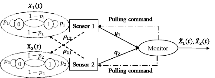
Figure 1: System model.

We consider a real-time tracking system consisting of two independent sources with corresponding sensors and a remote monitor, as shown in Fig. 1. Time is divided into discrete time slots, i.e., ${t\in\{0,1,\ldots\}}$.

The sources are indexed by $i\in\{1,2\}$. Each source $i$ is modeled as a two-state (binary) discrete-time Markov chain ${X_{i}(t)=\{0,1\}}$ with a symmetric transition probability matrix $P_{i}$. For clarity in presentation, we choose binary Markov sources, but our study can be easily extended to general finite Markov sources. This extension would, however, exponentially increase the dimension of the problem in the number of states of the sources.

Each source is observed by its dedicated sensor and potentially by the other sensor(s). This could happen due to direct communication between sensors (e.g., in vehicular communications) or overlapping sensor views (e.g., in smart factories where robots working in shared areas may detect each other’s positions or other related information). At each time slot, each sensor $i$ collects information about the state of source $i$. Additionally, with probability $\rho_{ij}$, the measurement collected by sensor $i$ also includes information about the current state of source $j$, $X_{j}(t)$. The overall correlation structure is captured by a matrix $\bm{\mathrm{P}}\triangleq[\rho_{ij}]$, where $\rho_{ij}\in[0,1]$ represents the probability that sensor $i$ observes source $j$, with $\rho_{ii}=1$ for all $i$. This type of correlation model is also used in [11, 12].

The status updating follows a pull-based protocol. At each time slot $t$, the monitor can pull (command) a sensor. The selected sensor then sends the status data to the monitor. Let $a(t)\in\{0,1,2\}$ denote the command action of the monitor at slot $t$, where $a(t)=0$ means the monitor is idle, and $a(t)=i,~i=1,2,$ means the monitor commands source $i$.

We assume an error-prone communication channel between each sensor and the monitor. Each transmission from sensor $i$ to the monitor occupies one time slot and is successfully received with probability ${q_{i}}$, referred to as the reception success probability.

The monitor generates a real-time estimate of each source $i$. Let us denote the estimate of source $i$ at slot $t$ by $\hat{X}_{i}(t)$ for all $i$. Noting that the construction of the estimate $\hat{X}_{i}(t)$ depends on the design performance metric, next, we first define our performance metric and then our estimation strategy.
As a goal-oriented metric, we consider a generic distortion measure defined as:

$$d_{i}(t)\triangleq f_{i}\left(X_{i}(t),\hat{X}_{i}(t)\right),$$ (1)

where the function ${f_{i}:\mathcal{X}_{i}\times\mathcal{X}_{i}\rightarrow\mathbb{R}}$ could be any bounded function, i.e., ${|f(.)|<\infty}$ [10], where $\mathcal{X}_{i}\in\{0,1\}$ is the state space of each source $i$. The function $f_{i}(\cdot)$ can represent different estimation error metrics. For example, it could be the squared estimation error, $d_{i}(t)=(X_{i}(t)-\hat{X}_{i}(t))^{2}$, or the real-time error, ${d_{i}(t)=\mathds{1}_{\{X_{i}(t)\neq\hat{X}_{i}(t)\}}}$, where the binary indicator function $\mathds{1}_{\{.\}}$ equals one if the input argument holds true.
As shown in [7], the estimation strategy, i.e., the construction of $\hat{X}_{i}(t)$, has significant impact on the scheduling policy and performance. We propose a minimum mean distortion estimation, where distortion could be any function as defined in (1). To compute the estimate, we require the probability distribution over the state space of the sources based on potentially all history of received samples and their time stamps. Since the sources are Markovian, the most recently received samples, along with their respective ages, provide sufficient information to obtain the estimate. The estimate can be computed as

$$\hat{X}_{i}(t)=\operatorname*{arg\,min}_{Y_{i}(t)\in\mathcal{X}_{i}}~\mathbb{E}\left\{f_{i}\left(X_{i}(t),\,Y_{i}(t)\right)\right\},$$ (2)

where the expectation is taken with respect to the probability distribution over $X_{i}(t)$.

At each time slot, the goal is to determine the optimal command action $a(t)$ for the monitor that minimizes a cost function. The cost function combines the average number of transmissions as a transmission cost and a weighted sum of distortions. Formally, this leads to the following stochastic control problem:

minimize $$\limsup_{T\rightarrow\infty}\frac{1}{T}\!\sum_{t=1}^{T}\mathbb{E}\!\left\{\sum_{i}w_{i}d_{i}(t)\!+\!\alpha\mathds{1}_{\{a(t)\neq 0\}\!}\right\},$$ (3)

where the variables are ${\{a(t)\}_{t=1,2,\ldots}}$. Here, $w_{i}$ represents the importance of source $i$, $\alpha$ is a coefficient that emphasizes the transmission cost, and $\mathbb{E}\{\cdot\}$ is the expectation operator taken over the randomness of the system (due to the sources, correlation, and wireless channel) and the (possibly randomized) action selection of $a(t)$.

III A Solution to Problem (3)

This section proposes a solution to problem (3). The sources $X_{i}(t)$ are not observable to the controller, and thus, we first model problem (3) as a POMDP. Then, we cast the POMDP into a finite-state MDP problem and solve it using RVIA.

The POMDP is described by the following elements:
$\bullet$ State: Let ${\delta_{i}(t)\in\{1,2,\dots\}}$ denote the age of the most recent sample $\bar{X}_{i}(t)$ of source $i$ received by the monitor before slot $t$. The state at slot $t$ is ${s(t)=\left\{X_{i}(t),\bar{X}_{i}(t),\delta_{i}(t)\right\}_{i=1,2}}$. The most recent samples $\bar{X}_{i}(t)$ and their ages $\delta_{i}(t)$ are included in the state because they are required to construct the estimate $\hat{X}_{i}(t)$, hence the cost function.
$\bullet$ Observation: The observation (at the monitor) at slot $t$ is ${O(t)=\left\{\bar{X}_{i}(t),\delta_{i}(t)\right\}_{i=1,2}}$.
$\bullet$ Action: The action at slot $t$ is $a(t)\in\{0,1,2\}$, as defined in Section II.
$\bullet$ State transition probabilities: The transition probabilities from current state ${s=\left\{X_{i},\bar{X}_{i},\delta_{i}\right\}_{i=1,2}}$ to next state ${s^{\prime}=\left\{X^{\prime}_{i},\bar{X}_{i}^{\prime},\delta_{i}^{\prime}\right\}_{i=1,2}}$ under a given action $a$ is defined by ${\Pr\{s^{\prime}\,|\,s,a\}}.$ Since the sources’ dynamics are independent, $\Pr\{s^{\prime}\,|\,s,a\}$ is given as

$$\Pr\{s^{\prime}\,|\,s,a\}=\Pr\left\{\bar{X}_{1}^{\prime},\,\bar{X}_{2}^{\prime},\,\delta_{1}^{\prime},\,\delta_{2}^{\prime}\,|\,s,\,a\right\}\prod_{i}\Pr\{X_{i}^{\prime}\,|\,X_{i}\},$$

where $\Pr\left\{\bar{X}_{1}^{\prime},\,\bar{X}_{2}^{\prime},\,\delta_{1}^{\prime},\,\delta_{2}^{\prime}\,|\,s,\,a\right\}$ is given by (5) on the top of the next page, and

$$\begin{array}[]{cc}\Pr\{X_{i}^{\prime}\,|\,X_{i}\}=\left\{\begin{array}[]{ll}p_{i},&\text{if}~X_{i}^{\prime}=X_{i},\\ 1-p_{i},&\text{if}~X_{i}^{\prime}\neq X_{i},\\ 0,&\text{otherwise}.\end{array}\right.\end{array}$$ (4)

$$\begin{array}[]{ll}&\Pr\left\{\bar{X}_{1}^{\prime},\,\bar{X}_{2}^{\prime},\,\delta_{1}^{\prime},\,\delta_{2}^{\prime}\,|\,s,\,a\right\}=\left\{\begin{array}[]{ll}1,&\text{if}~a=0,~\bar{X}_{1}^{\prime}=\bar{X}_{1},~\bar{X}_{2}^{\prime}=\bar{X}_{2},~\delta_{1}^{\prime}=\delta_{1}+1,~\delta_{2}^{\prime}=\delta_{2}+1,\\ 1-q_{1},&\text{if}~a=1,~\bar{X}_{1}^{\prime}=\bar{X}_{1},~\bar{X}_{2}^{\prime}=\bar{X}_{2},~\delta_{1}^{\prime}=\delta_{1}+1,~\delta_{2}^{\prime}=\delta_{2}+1,\\ 1-q_{2},&\text{if}~a=2,~\bar{X}_{1}^{\prime}=\bar{X}_{1},~\bar{X}_{2}^{\prime}=\bar{X}_{2},~\delta_{1}^{\prime}=\delta_{1}+1,~\delta_{2}^{\prime}=\delta_{2}+1,\\ q_{1}\rho_{12},&\text{if}~a=1,~\bar{X}_{1}^{\prime}=X_{1},~\bar{X}_{2}^{\prime}=X_{2},~\delta_{1}^{\prime}=1,~\delta_{2}^{\prime}=1,\\ q_{1}(1-\rho_{12}),&\text{if}~a=1,~\bar{X}_{1}^{\prime}=X_{1},~\bar{X}_{2}^{\prime}=\bar{X}_{2},~\delta_{1}^{\prime}=1,~\delta_{2}^{\prime}=\delta_{2}+1,\\ q_{2}\rho_{21},&\text{if}~a=2,~\bar{X}_{1}^{\prime}=X_{1},~\bar{X}_{2}^{\prime}=X_{2},~\delta_{1}^{\prime}=1,~\delta_{2}^{\prime}=1,\\ q_{2}(1-\rho_{21}),&\text{if}~a=2,~\bar{X}_{1}^{\prime}=\bar{X}_{1},~\bar{X}_{2}^{\prime}=X_{2},~\delta_{1}^{\prime}=\delta_{1}+1,~\delta_{2}^{\prime}=1,\\ 0,&\text{otherwise}.\end{array}\right.\end{array}$$ (5)

 

$\bullet$ Observation function: The observation function is the probability distribution function of $o(t)$ given state $s(t)$ and action $a(t-1)$, i.e., ${\Pr\{o(t)\,\big{|}\,s(t),a(t-1)\}}$. Since the observation is always part of the state, the observation function is deterministic, i.e., ${\Pr\{o(t)\,\big{|}\,s(t),a(t-1)\}=\mathds{1}_{\{o(t)=\left\{\bar{X}_{i}(t),\delta_{i}(t)\right\}_{i=1,2}\}}}$.
$\bullet$ Cost function: The immediate cost function at slot $t$ is

$$C(s(t),a(t))=\sum_{i}w_{i}d_{i}(t)+\alpha\mathds{1}_{\{a(t)\neq 0\}}.$$ (6)

Now, with the POMDP specified above, we follow the belief MDP approach [16, Ch. 7] to achieve an optimal decision-making for the POMDP. Accordingly, in the sequel, we transform the POMDP into a belief MDP.
Let $I_{\mathrm{C}}(t)$ denote the complete information state at slot $t$ consisting of [16, Ch. 7]: i) the initial probability distribution over the state space, ii) all past and current observations, $o(0),\dots,o(t)$, and iii) all past actions, $a(0),\dots,a(t-1)$. The belief is a probability distribution over the source state space. We define the belief for each source $i$ at slot $t$ as

$$b_{i}(t)\triangleq\Pr\{X_{i}(t)=1\,\big{|}\,I_{\mathrm{C}}(t)\},~\forall\,i.$$ (7)

The belief at $t+1$ is updated after performing action $a(t)$ and receiving observation $o(t+1)$. The belief update is given as:

$$\hskip-15.00002pt\begin{array}[]{ll}&b_{i}(t+1)=\\ &\left\{\begin{array}[]{ll}p_{i}&\text{if}~\delta_{i}(t+1)=1,~\bar{X}_{i}(t+1)=1\\ 1-p_{i}&\text{if}~\delta_{i}(t+1)=1,~\bar{X}_{i}(t+1)=0,\\ b_{i}(t)p_{i}+(1-b_{i}(t))\bar{p_{i}},&\text{if}~\delta_{i}(t+1)\neq 1.\end{array}\right.\end{array}$$ (8)

where $\bar{p_{i}}\triangleq 1-p_{i}$. The belief state is then defined by

$$z(t)\triangleq\left\{b_{i}(t),\bar{X}_{i}(t),\delta_{i}(t)\right\}_{i=1,2}$$ (9)

Having the belief state defined, we can formulate the belief MPD problem. However, solving the resulting (belief) MDP problem is challenging because the belief is a continuous state variable, and thus, the state space of the problem is infinite. Nonetheless, from the evolution of belief in (8) we can observe that the last line in the equation is the propagation of uncertainty in the associated Markov chain, where the value of $\delta_{i}(t)$ indicates how many transitions happened from the last time the source state was $\bar{X}_{i}(t)$. This argument suggests that we can equivalently rewrite the belief in (8), based on the $N$-step transition probabilities formula [17], as follows:

$$\hskip-10.00002pt\begin{array}[]{ll}&b_{i}(t+1)=\left\{\begin{array}[]{ll}0.5\left(1+(2p_{i}-1)^{\delta_{i}(t+1)}\right)&\text{if}~\bar{X}_{i}(t+1)=1\\ 0.5\left(1-(2p_{i}-1)^{\delta_{i}(t+1)}\right)&\text{if}~\bar{X}_{i}(t+1)=0.\end{array}\right.\end{array}$$ (10)

From (10), we can observe that for sufficiently large values of $\delta_{i}(t)$, i.e., $\delta_{i}(t)\geq N$, the belief approaches $0.5$ exponentially as $\delta_{i}(t)$ increases. This implies that we can re-define the state (9) as

$$\underline{z}(t) =$$ (11)

$$\left\{\bar{X}_{i}(t),\delta_{i}(t)\right\}_{i=1,2},\,\bar{X}_{i}(t)\in\{0,1\},\delta_{i}(t)\in\{1,\dots,N\},$$

and formulate a finite-state MDP problem.

Note that the action of the above-mentioned finite-state MDP problem remains the same as that of the POMDP. Moreover, the state transition probabilities are given by

$$\begin{array}[]{cc}\displaystyle\Pr\{\underline{z}^{\prime}\,|\,\underline{z},a\}=\sum_{X_{i}\in\{0,1\}}\Pr\{\underline{z}^{\prime}\,|\,\underline{z},a,X_{1},X_{2}\}\Pr\{X_{1},X_{2}\,|\,\underline{z},a\},\end{array}$$ (12)

where $\Pr\{\underline{z}^{\prime}\,|\,\underline{z},a,X_{1},X_{2}\}$ can be obtained by (5), and due to the independency between the dynamic of sources, $\Pr\{X_{1},X_{2}\,|\,\underline{z},a\}$ can be written as $\displaystyle{\Pr\{X_{1},X_{2}\,|\,\underline{z},a\}=\prod_{i\in\{1,2\}}\Pr\{X_{i}\,|\,\underline{z},a\}}$, where

$$\begin{array}[]{ll}&\Pr\{X_{i}\,|\,\underline{z},a\}=\\ &\left\{\begin{array}[]{ll}0.5\left(1+(2p_{i}-1)^{\delta_{i}(t)}\right),&\text{if}~~X_{i}=1,~\bar{X}_{i}=1,\\ 0.5\left(1-(2p_{i}-1)^{\delta_{i}(t)}\right),&\text{if}~~X_{i}=0,~\bar{X}_{i}=1,\\ 0.5\left(1+(2p_{i}-1)^{\delta_{i}(t)}\right),&\text{if}~~X_{i}=0,~\bar{X}_{i}=0,\\ 0.5\left(1-(2p_{i}-1)^{\delta_{i}(t)}\right),&\text{if}~~X_{i}=1,~\bar{X}_{i}=0.\end{array}\right.\end{array}$$ (13)

Finally, the immediate cost function is

$$C(t)=$$

$$\sum_{i}w_{i}\left(b_{i}(t)f(1,\hat{X}_{i}(t))+(1-b_{i}(t))f(0,\hat{X}_{i}(t))\right)$$

$$+\alpha\mathds{1}_{\{a(t)\neq 0\}},$$ (14)

where $b_{i}(t)$ is given by (8), and the estimate $\hat{X}_{i}(t)$ is obtained according to minimum mean distortion estimation, using the ages $\delta_{i}(t)$ and the last sample $\bar{X}_{i}(t)$ given in the state $\underline{z}(t)$.

Due to the source dynamics and the chance of loss in the channels, it is not difficult to see that the above-formulated MDP is unichain. Furthermore, the MDP is also aperiodic. Shortly, these follow because the state $(0,0,N,N)$ can be accessible from any state, including itself, under any stationary deterministic policy. By unichain and aperiodicity properties of the MDP, we apply RVIA to obtain an optimal policy, which is guaranteed to converge [18].

IV Numerical Results

This section presents simulation results to demonstrate the effectiveness of the derived policy and the impact of various parameters on the system’s performance. The RVIA stopping criterion is set to $10^{-3}$, the weights of both sources, $w_{1}$ and $w_{2}$, are set to $1$, and the distortion metric defaults to real-time error unless stated otherwise. Other parameters are provided in the captions of the corresponding figure. For benchmarking, we consider two commonly used policies: 1) Max-age-first: this policy commands the sensor whose direct observing source has the highest age at the monitor. 2) Age-optimal: this policy is derived by replacing the distortion, $d_{i}(t)$, with the AoI at the monitor, $\delta_{i}(t)$, in the objective function (3) and solving the resulting problem.

We first analyze the effect of the coefficient factor $\alpha$ in (3) (i.e., the transmission cost) on the average weighted total cost, as shown in Fig. 2. The results indicate that the proposed policy significantly outperforms the baseline policies, particularly as the transmission cost increases. This improvement occurs because the max-age-first policy ignores transmission costs, and the age-optimal policy is source-agnostic and may initiate transmissions even when the source state matches its estimate at the monitor. Additionally, Fig. 2 shows that the performance of the proposed policy remains nearly constant beyond a certain point. This is because when the transmission cost is high, the optimal action for the monitor is to remain idle, leading to maximum distortion irrespective of $\alpha$.

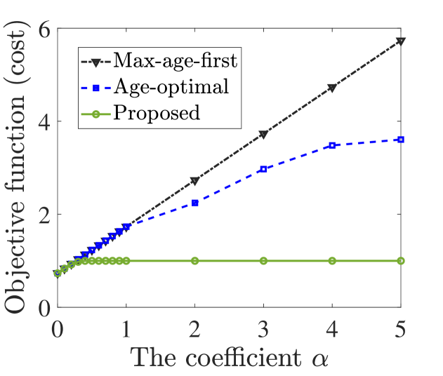
Figure 2: The average cost (the objective function in (3)) vs. the coefficient $\alpha$ (transmission cost) for $p_{1}=0.7$, $p_{2}=0.7,$ $q_{1}=0.8$, $q_{2}=0.6,$ $\rho_{12}=0.4$, and $\rho_{21}=0.7$.

Fig. 3 shows the average cost as a function of the observation correlations, assumed equal for both sources ($\rho_{12}=\rho_{21}$), for two different distortion functions: 1) the real-time error in Fig. 3(a), and 2) a distortion given by (15) in Fig. 3(b). The results indicate that as correlation probabilities increase, the average cost decreases for both distortion functions, especially when channel conditions are good ($q_{1}$ and $q_{2}$ are, e.g., more than $0.9$). This is because a higher correlation provides a higher chance to update the monitor about the other source’s state as well, which in turn corrects the sources’ estimates and reduces the distortion. Furthermore, the figures show that for both real-time error distortion and the distortion in (15), the age-optimal and max-age-first policies perform almost identically, while there is a notable gap between these baseline policies and the proposed optimal policy.

$$d_{1}=\begin{bmatrix}0&30\\ 10&0&\end{bmatrix},~~~~~~~~\\ d_{2}=\begin{bmatrix}0&10\\ 50&0&\end{bmatrix}.$$ (15)

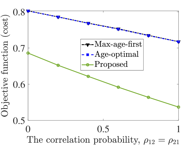
(a) The real-time error

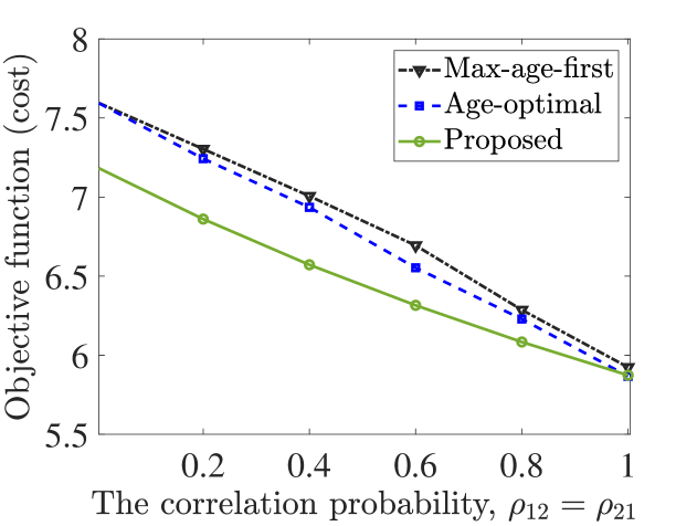
(b) The distortion given by (15)

Figure 3: The average cost vs. the correlation probabilities for different distortions for $p_{1}=0.9$, $p_{2}=0.9$, $q_{1}=0.9$, $q_{2}=0.9$, and $\alpha=0.5$.

Fig. 4 illustrates the average cost as a function of the self-transition probabilities of the sources, $p_{1}$ and $p_{2}$, for different policies. The figure highlights a symmetric behavior of the cost function, with the maximum cost occurring at $p_{1}=p_{2}=0.5$, where the sources have the maximum entropy, making them harder to track accurately. This symmetric behavior is expected due to the trackability of sources that are either slow-varying, i.e., high $p_{1}$ and $p_{2}$, or fast-varying, i.e., low $p_{1}$ and $p_{2}$, provided that an appropriate optimal estimation strategy is used. However, if the estimation strategy does not adapt to the source dynamics, such as using a fixed last-sample estimate, the performance degrades significantly, particularly for the fast-varying sources. The performance gap between the proposed optimal policy and the baseline policies is most pronounced at $p_{1}=0.5$ and $p_{2}=0.5$, as the baseline policies are source-agnostic. Nonetheless, the symmetric behavior of the baseline policies persists because their estimation strategy adapts adequately to the source dynamics.

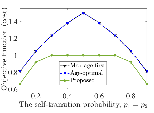
Figure 4: The average cost vs. the self-transition probabilities of the sources for $q_{1}=0.8$, $q_{2}=0.6,$ $\rho_{12}=0.4$, $\rho_{21}=0.7$, and $\alpha=0.5$.

Fig. 5 examines the impact of channel reliability on the performance of different policies with $q_{1}=q_{2}$. The results show a direct relationship between cost reduction and channel reliability: a higher channel reliability leads to a lower cost. This is because, by increasing the reliability, the likelihood of successful transmissions increases, enabling the monitor to stay informed about the source states and track them more accurately. The figure also shows that the baseline policies perform similarly, while the proposed policy consistently outperforms them.

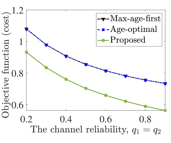
Figure 5: The average cost vs. the channel reliabilities for $p_{1}=0.9$, $p_{2}=0.9$, $\rho_{12}=0.8$, $\rho_{21}=0.8$, and $\alpha=0.5$.

V Conclusions

We studied a goal-oriented real-time remote tracking problem in a status updating system with correlated observations, comprising two independent Markov sources, two sensors, and a monitor. We aimed to find the optimal pull policy for the monitor to minimize the weighted sum of distortion and transmission costs. Using a POMDP-based approach, we formulated the problem as a belief-MDP. Then, by expressing the belief as a function of AoI, we cast a finite-state MDP problem and solved it via RVI.

The simulation results showed that the derived policy outperforms the baseline policies, max-age-first and age-optimal, in cost reduction, while he baseline policies showed similar performance in most cases. Results also indicated that the correlation reduces distortion, which is symmetric around the self-transition probability being $0.5$. While we addressed correlation in the observations, exploring the correlation in the sources’ dynamics remains an open problem for future work.

References

- [1] D. Gündüz et al., “Beyond transmitting bits: Context, semantics, and task-oriented communications,” IEEE J. Sel. Areas Commun., vol. 41, no. 1, pp. 5–41, Jan. 2023.
- [2] A. Zakeri, Information Freshness Optimization and Semantic-Aware Status Updating. Oulun Yliopisto, 2024.
- [3] E. Uysal et al., “Semantic communications in networked systems: A data significance perspective,” IEEE Netw., vol. 36, no. 4, pp. 233–240, Jul. 2022.
- [4] M. Kountouris and N. Pappas, “Semantics-empowered communication for networked intelligent systems,” IEEE Commun. Mag., vol. 59, no. 6, pp. 96–102, Jun. 2021.
- [5] M. Salimnejad, M. Kountouris, and N. Pappas, “Real-time reconstruction of Markov sources and remote actuation over wireless channels,” IEEE Trans. Commun., vol. 72, no. 5, pp. 2701–2715, May 2024.
- [6] A. Li, S. Wu, S. Meng, R. Lu, S. Sun, and Q. Zhang, “Toward goal-oriented semantic communications: New metrics, framework, and open challenges,” IEEE Wireless Commun., vol. 31, no. 5, pp. 238–245, Oct. 2024.
- [7] A. Zakeri, M. Moltafet, and M. Codreanu, “Goal-oriented remote tracking of an unobservable multi-state Markov source,” in Proc. IEEE Wireless Commun. and Networking Conf., Dubai, UAE, Apr. 2024.
- [8] E. Fountoulakis, N. Pappas, and M. Kountouris, “Goal-oriented policies for cost of actuation error minimization in wireless autonomous systems,” IEEE Commun. Lett., vol. 27, no. 9, pp. 2323–2327, Sep. 2023.
- [9] P. M. de Sant Ana, N. Marchenko, B. Soret, and P. Popovski, “Goal-oriented wireless communication for a remotely controlled autonomous guided vehicle,” IEEE Wireless Commun. Lett., vol. 12, no. 4, pp. 605–609, Apr. 2023.
- [10] A. Zakeri, M. Moltafet, and M. Codreanu, “Semantic-aware sampling and transmission in real-time tracking systems: A POMDP approach,” IEEE Trans. Commun., Early Access, Dec. 2024.
- [11] V. Tripathi and E. Modiano, “Optimizing age of information with correlated sources,” in Proc. of the Int. Symp. on Theory, Algorithmic Foundations, and Protocol Design for Mobile Netw. and Mobile Comp., MobiHoc ’22, pp. 41–50, Mar. 2022.
- [12] E. Erbayat, A. Maatouk, P. Zou, and S. Subramaniam, “Age of information optimization and state error analysis for correlated multi-process multi-sensor systems,” in Proc. of the Int. Symp. on Theory, Algorithmic Foundations, and Protocol Design for Mobile Netw. and Mobile Comp., MobiHoc ’24, p. 331–340, Oct. 2024.
- [13] A. E. Kalør and P. Popovski, “Timely monitoring of dynamic sources with observations from multiple wireless sensors,” IEEE/ACM Trans. Netw., vol. 31, no. 3, pp. 1263–1276, Jun. 2023.
- [14] P. Agheli, N. Pappas, P. Popovski, and M. Kountouris, “Integrated push-and-pull update model for goal-oriented effective communication,” arXiv preprint arXiv:2407.14092, Jul. 2024.
- [15] I. Cosandal, S. Ulukus, and N. Akar, “Joint age-state belief is all you need: Minimizing AoII via pull-based remote estimation,” arXiv preprint arXiv:2411.07179, Nov. 2024.
- [16] O. Sigaud and O. Buffet, Markov decision processes in artificial intelligence. John Wiley & Sons, 2013.
- [17] C. Kam, S. Kompella, G. D. Nguyen, J. E. Wieselthier, and A. Ephremides, “Towards an effective age of information: Remote estimation of a Markov source,” in Proc. IEEE INFOCOM Workshop, pp. 367–372, Honolulu, HI, USA, Apr. 2018.
- [18] A. Zakeri, M. Moltafet, M. Leinonen, and M. Codreanu, “Minimizing the AoI in resource-constrained multi-source relaying systems: Dynamic and learning-based scheduling,” IEEE Trans. Wireless Commun., vol. 23, no. 1, pp. 450–466, Jan. 2024.