Extended Fractional Chern Insulators Near Half Flux in Twisted Bilayer Graphene Above the Magic Angle

Abstract

Fractional Chern insulators (FCIs)—the lattice analog of the fractional quantum Hall states—form as fractionalized quasiparticles emerge in a partially-filled Chern band. This fractionalization is driven by an interplay of electronic interaction and quantum geometry of the underlying wavefunctions. Bilayer graphene with an interlayer twist near the magic angle of 1.1°  hosts diverse correlated electronic states at zero magnetic field. When the twist angle exceeds 1.3°, the electronic bandwidth is sufficient to suppress the zero-field correlated states. Yet applying a magnetic field can restore the importance of electron-electron interactions. Here, we report strongly-correlated phases when a 1.37° twisted bilayer graphene sample is tuned to near half a magnetic flux quantum per moiré cell, deep into the Hofstadter regime. Most notably, well-quantized odd-denominator FCI states appear in multiple Hofstadter subbands, over unusually large ranges of density. This suggests a mechanism beyond disorder is stabilizing the fractional states. We also observe a bending and resetting of the Landau minifan reminiscent of the cascade of Dirac resets observed in magic-angle samples near integer filling at zero field.

Introduction

Twisted bilayer graphene (TBG), the archetypal strongly-correlated moiré heterostructure, displays an astonishingly diverse set of correlated electronic and topological phases [1, 2, 3, 4, 5, 6, 7, 8, 9, 10, 11, 12]. The electronic moiré miniband structure depends sensitively and predictably on the twist angle. Near the magic angle of 1.1°, the large moiré length scale enables tuning the density of charge carriers through entire minibands and the density of magnetic flux to on order one flux quantum $\Phi_{0}=e/h$ per moiré cell, where $e$ is the elementary charge and $h$ is Planck’s constant. In this “Hofstadter’s butterfly” regime [13, 14, 15, 16, 17, 18, 19, 11, 20, 21, 22, 23, 24], the energy spectrum exhibits a fractal structure with field-induced topological subbands. Gaps in the fractal spectrum appear at fluxes and densities described by Diophantine equations of the form $n/n_{s}=s+t\Phi/\Phi_{0}$ [25]. Here, $n_{s}=1/A$, $\Phi=BA$, $A$ is the moiré unit cell area, $B$ is the magnetic field normal to the plane of the samples, $s$ is the density offset at zero flux, and $t$ is the Chern number associated with the gap. We notate these Středa lines as $(s,\ t)$. Within such a gap, the Hall conductance is expected to be quantized to $\sigma_{xy}=te^{2}/h$ [26].

Integer $t$ Středa lines have been observed in TBG at a range of twist angles. Some of these states are not describable by single-particle models, as symmetries are broken by electronic interactions [27, 7, 12, 22, 24]. Středa lines with fractional $t$ and nonzero $s$ are more exotic and are referred to as fractional Chern insulators (FCIs). Analogous to fractional quantum Hall (FQH) states, where $s=0$, FCIs host fractionalized excitations [28]. Only a few examples of such states in moiré materials have been experimentally reported: twisted MoTe₂  [29, 30, 31] and multilayer twisted graphene aligned with hexagonal boron nitride (hBN)  [19, 8, 32, 33].

TBG’s viability as a platform for FCIs remains an open question [34]. Recently, fractional $t$ states have been observed in high-quality magic-angle TBG [35]. These occurred in Landau levels originating from charge neutrality ($s=0$), reminiscent of ordinary FQH. So far, FCIs with $s\neq 0$ have not been clearly demonstrated in experiments on TBG devices not aligned to hBN.

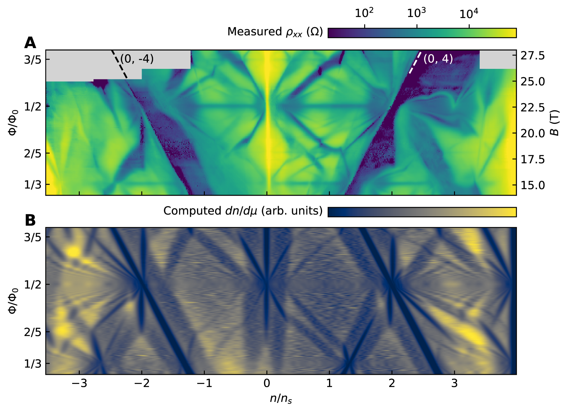
Figure 1: Strained TBG in the Hofstadter butterfly regime. (A) Dependence of the longitudinal resistance as a function of density and field. We indicate Středa lines $(s,\ t)=(0,\,\pm 4)$ with dashed lines. The metallic top gate began to leak to the TBG above 25 T, so we reduced its voltage range, leaving the greyed out regions. See the supplement for a schematic description of quantum Hall gaps (Fig. S1), the behavior of other contact pairs (Figs. S2 and S3), a comparison with the lower-field data presented in Ref. [36] (Fig. S4), and a schematic of the device with our inferred twist angles as extracted from the Landau fan diagram (Fig. S5). (B) Computed density of states d$n$/d$\mu$ for the spectrum in Fig. 3A with an arbitrary linear color map. Gaps show up as dark lines. See Sec. III for details on the computation.

In Refs. [36] and [37], we presented magnetotransport measurements and single-particle calculations for a TBG sample twisted to near 1.37°, where the miniband width is large enough (near 100 meV) to suppress correlated electronic states near zero magnetic field [1, 3, 36]. In this work, we further explore that same sample, now at extremely high magnetic fields, demonstrating many $B$-induced strongly correlated states. Most notably, at magnetic flux near half a magnetic flux quantum per moiré unit cell we observe plateaus in Hall resistance corresponding to $\pm 8/3$ and $-8/5$, quantized to within a few tenths of a percent, along with possible $-4/3$ plateaus. The $\pm 8/3$ plateaus in particular extend over a strikingly broad range of density, up to half an electron per moiré unit cell, rather than following a narrow, well-defined Středa line. Integer quantized states have been known to extend over a broad range of densities, outcompeting fractional states that might be expected at those densities. This “re-entrant quantum Hall effect” has been explained as a consequence of a Wigner crystal coexisting with a filled Landau level [38, 39], a scenario originally termed a partial Hall crystal [40]. However, in the sample we study here the integer states are less robust and broad than the $8/3$ fractional states. In Sec. V we discuss several mechanisms that might be responsible for the novel and surprising extended FCI regions.

I Longitudinal transport

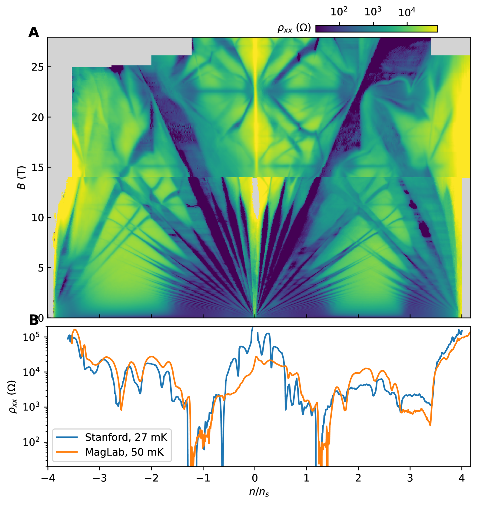
Figure S4: Full Landau fan including data taken at lower field. Contact pair 7 - 8. (A) Data from 0 to 14 T are taken in our system at Stanford, previously published in Ref. [36]. Data above 14 T are the same as in Fig. 1, taken at MagLab. (B) Line cuts from both systems at 14 T.

In the sample we study, longitudinal resistivity as a function of carrier density and magnetic field between 14 and 28 T ranges from below our measurement floor of a few ohms within quantum Hall gaps to hundreds of kilohms at band edges and near charge neutrality (Fig. 1A). Here, we focus on specific contact pairs within this 20-terminal Hall bar that demonstrated the sharpest low-field transport in Ref. [36]. For our twist angle of 1.37°, $\Phi/\Phi_{0}=1$ occurs at nearly 45 T, so the field range in our measurement corresponds to flux ratios between 0.31 and 0.62. We indicate the most prominent Středa lines, $(s,\ t)=(0,\,\pm 4)$, which persist without closing down to near-zero field (Fig. S4).

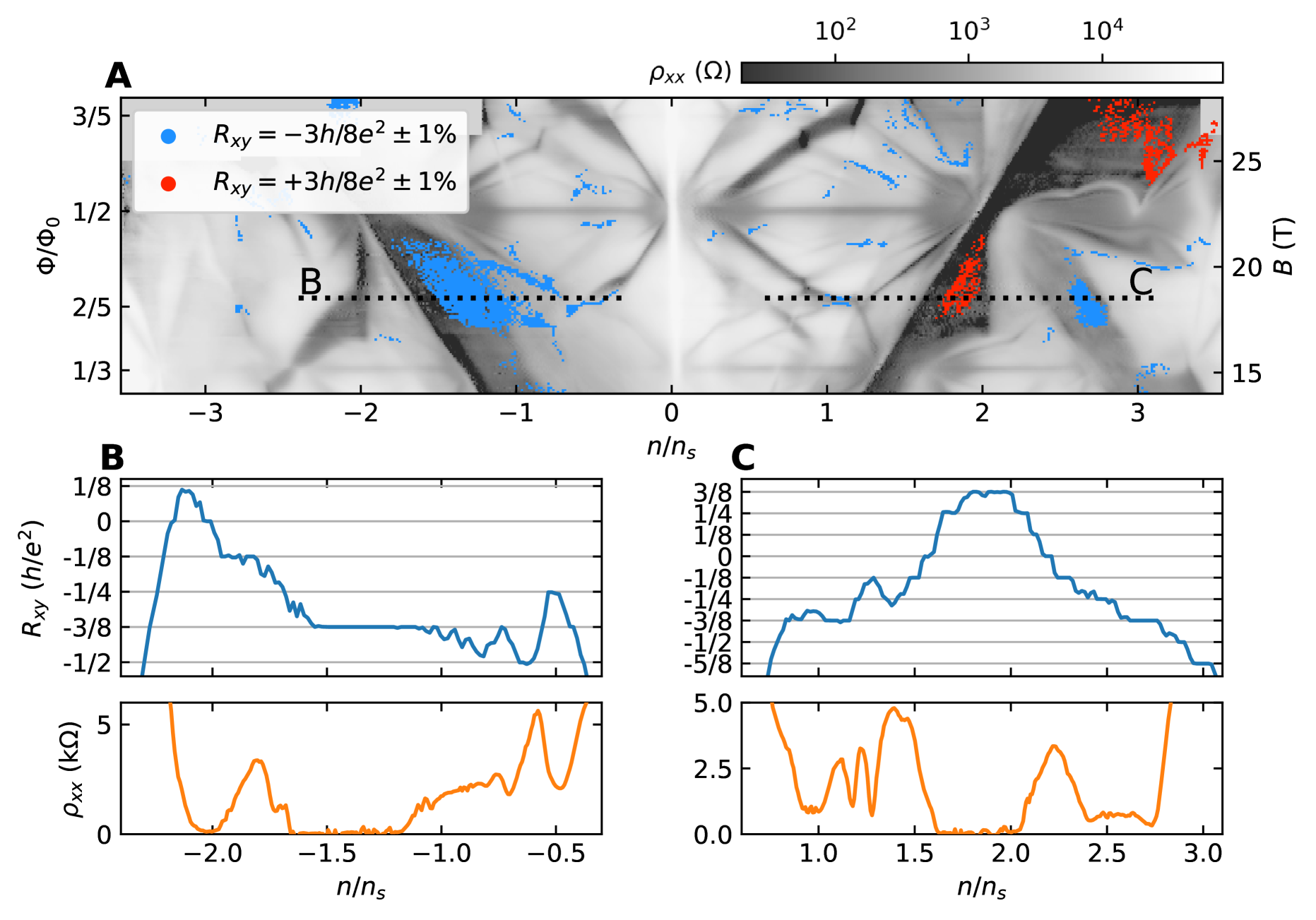
Figure 2: Fractional Chern insulating Hall plateaus. (A) Longitudinal resistance from Fig. 1 replotted in grey-scale. Superimposed on the longitudinal resistance are locations where the Hall resistance for a neighboring contact pair is quantized to within 1% of $\pm 8/3$ in red and blue, respectively. A clustering algorithm has been applied to remove spurious points (see Sec. S3). The abrupt loss of quantization at $\Phi/\Phi_{0}$ between $1/3$ and $2/5$ corresponds to a pause in the measurement of several hours. This, along with the noise above $1/2$, are described in Sec. S2. (B, C) Hall resistance and longitudinal resistivity as a function of density at 18.5 T ($\Phi/\Phi_{0}=0.41$, black dashed lines in A).

For comparison, we show the computed Wannier plot in the same field range (Fig. 1B). The computed density of states $dn/d\mu$ should show patterns similar to those seen in resistivity, but we do not directly calculate transport from our model as we did in [37] for lower magnetic fields. Our model broadly captures the splitting and bending behavior of the Landau levels emitting from half flux and $n/n_{s}=0$, where open orbits from uniaxial heterostrain and Zeeman splitting play the role of anisotropic hopping and energetic splitting as described in Ref. [36]. The model predicts a number of prominent gaps that we discuss in Sec. III.

In the supplementary materials we describe other striking phenomena such as Brown-Zak oscillations, symmetry-broken Chern insulating Středa lines with $s=\pm 1/2$, $t=\pm 3$, and correlated Hofstadter ferromagnets.

II Fractional Chern Insulators

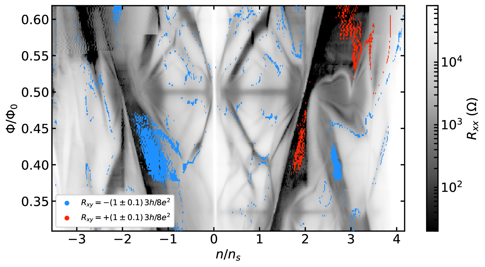
Figure S21: Raw Hall data. Unfiltered version of Fig. 2.

In Fig. 2A, we overlay in blue and red the regions where the Hall resistance is quantized to within 1% of $-3h/8e^{2}$ and $+3h/8e^{2}$ respectively. We apply an intentionally-conservative clustering threshold algorithm so that almost all of the pockets marked with color represent well-quantized plateaus of $\pm 8/3$ rather than regions where the Hall resistance incidentally passes through quantized values. These fractional Hall plateaus coincide with low longitudinal resistance (shown in gray). See Sec. S3 for details and Fig. S21 for unfiltered data.

Fig. 2 panels B and C show line cuts of $R_{yx}$ and $R_{xx}$ at 18.5 T. In addition to the aforementioned $\pm 8/3$ plateaus, a number of integer plateaus are visible, along with a small $-8/5$ plateau. Strikingly, the $\pm 8/3$ plateaus are quantized over larger ranges of density and field than any integer state. For a discussion of the degree of quantization, other fractions, and the behavior in other contact pairs, see Secs. S10,  S11, and  S7, respectively.

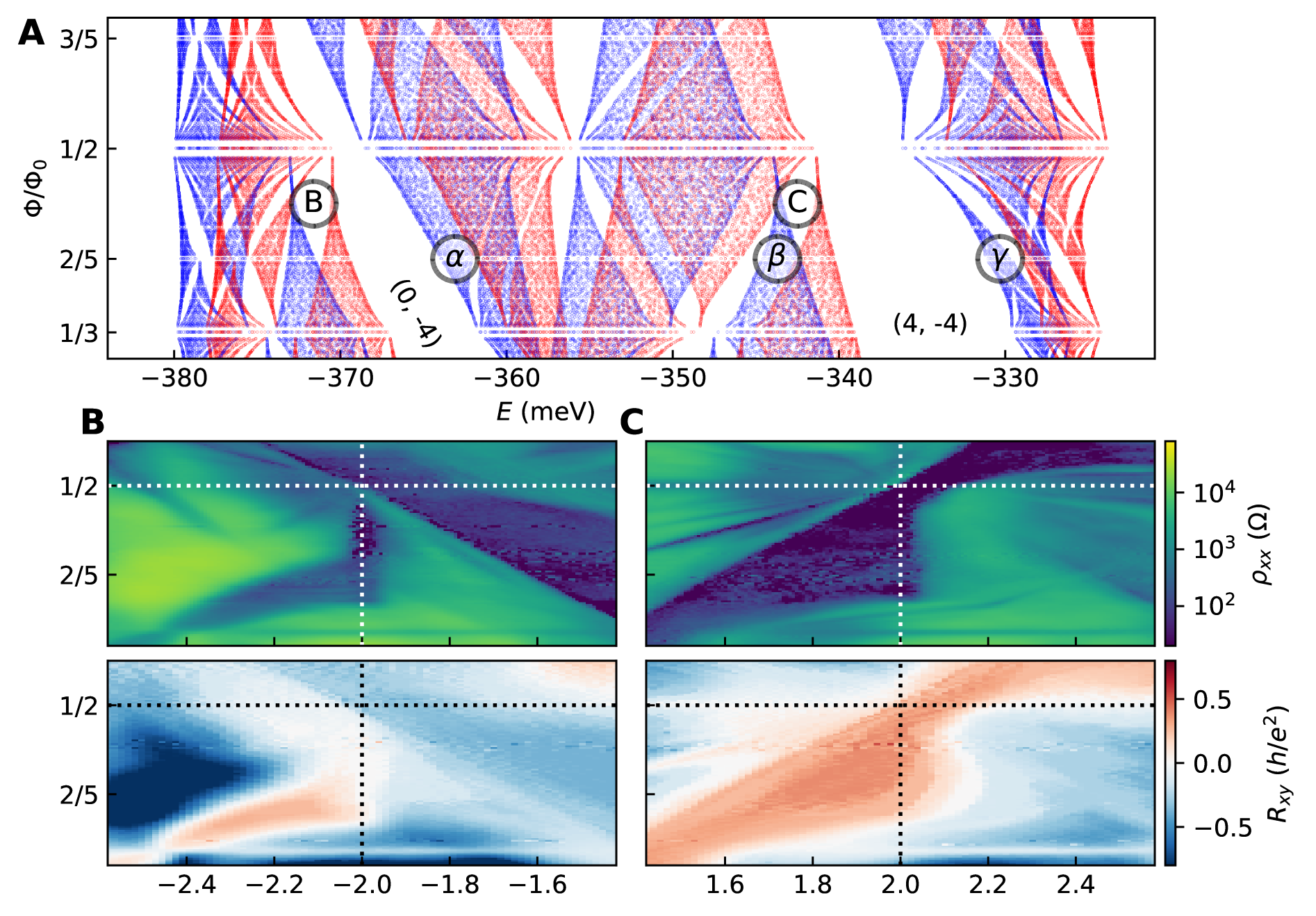
Figure 3: Computed Hofstadter spectrum and candidate quantum spin Hall state. (A) Computed energy levels for valley K, $\theta=1.35^{\circ}$ with $0.24\%$ uniaxial heterostrain at 45° and $0.3\%$ biaxial heterostrain ($q\leq 72$), as described in the text. Spin up electrons are shown in blue, and spin down electrons are shown in red. The gaps at $(s,t)=(0,-4)$ and $(4,-4)$ are labeled. $\alpha$, $\beta$, and $\gamma$ indicate the Hofstadter subbands which host the largest pockets of $\pm 8/3$ quantization shown in Fig. 2. Because of the Zeeman spin-splitting, it is possible for the net spin of all filled bands associated with a given gap to be non-zero. A trivial gap (t=0) with a net spin is reminiscent of quantum spin Hall. Two such gaps are indicated: (0, $\pm 2$). See Fig. S20 for the full range of fields. (B-C) Dependence of the longitudinal resistance (top panels) and Hall resistance (bottom panels) as a function of density and field centered on the two quantum spin Hall candidate gaps predicted from (A). In (B), below half flux, we observe a strong vertical suppression of longitudinal resistance coincident with a small plateau of zero Hall resistance at $n/n_{s}=-2$. In (C), we observe low longitudinal resistance along a vertical line, however the Hall resistance is not zero at the same densities.

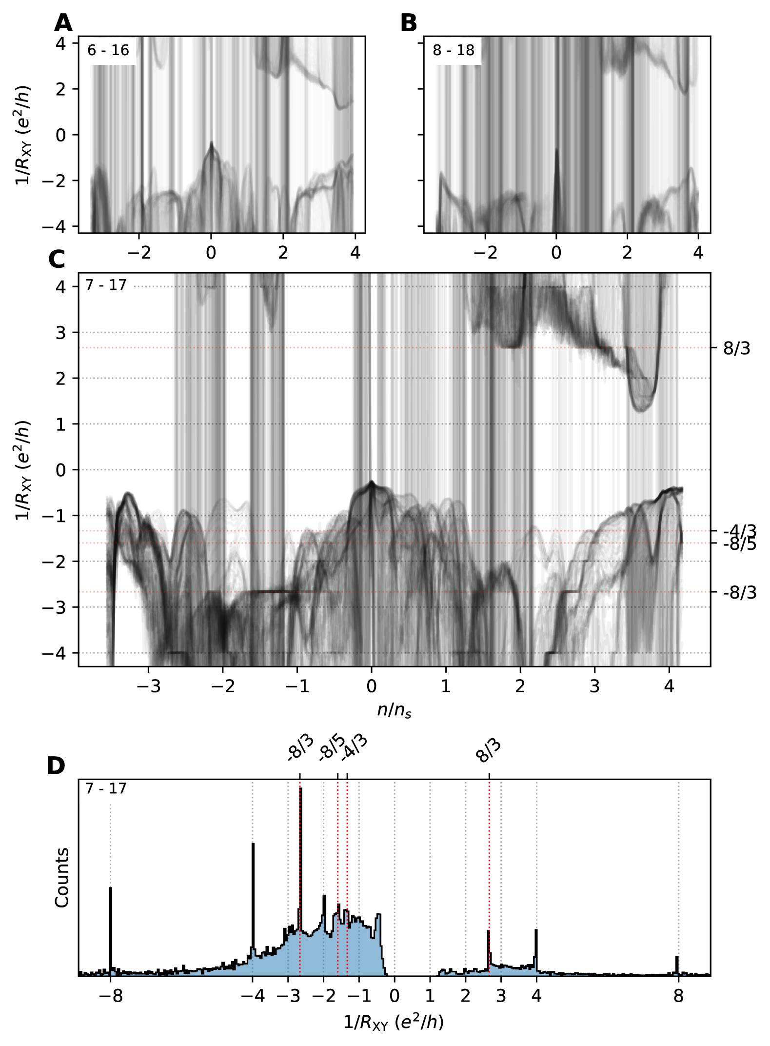
Figure S7: Hall plateaus. All line cuts at constant field of a Landau fan for a given contact pair plotted over each other with transparency. Quantized Hall plateaus will appear as solid horizontal lines. Contact pairs indicated in the top left corner. (A, B) There are no quantized Hall plateaus for these contact pairs, not even integers. (C) Contact pair 7 - 17 shows quantized plateaus at integers $\pm 8$ (not shown), $\pm 4$, -2, -8/3, -8/5, and -4/3, the latter two only near $n/n_{s}=3$. (D) Histogram of all Hall conductances. Interestingly, there are more -8/3 measurements than any integer.

Regions where the Hall resistance is (fractionally) quantized typically coincide with suppressed longitudinal resistance in the four adjacent contact pairs (see Fig. 1 and Sec. S7). Though measurements from neighboring longitudinal probes vary subtly, neighboring Hall probes exhibit strikingly different behavior: those just 3 microns away from the main Hall pair we focus on in this manuscript exhibit poor quantization, even for integer quantum Hall states (Fig. S7), possibly due to mixing of the longitudinal resistance into the Hall measurement because of spatial variation in twist angle . We therefore suspect that the main Hall pair of this manuscript contacts a region of unusually high moiré uniformity.

We defer a detailed discussion of potential explanations of the extended fractional phenomenology to Sec. V.

III Hofstadter Model

To understand the Hofstadter bands we would expect without interactions we perform bandstructure computations within a single-particle model. Our effective continuum model from Ref. [37] which accounted for uniaxial heterostrain can be extended into the Hofstadter regime [42]. Here we also incorporate biaxial heterostrain, lattice relaxation, and electron-hole asymmetry so that the locations of the three van Hove points near $B=0$ on the hole side of the charge neutrality point differ from those on the electron side [43, 44], as is seen in the experiment [36, 37]. We fully parameterize the $2\times 2$ moiré deformation matrix as a function of twist angle, uniaxial heterostrain magnitude and direction, and biaxial heterostrain magnitude. We then search for structural parameters that yield bands with van Hove points at densities matching those identified in Ref. [37]. We find a unique best fit—$0.24\pm 0.02$% uniaxial heterostrain at $45\pm 4$° and $0.3\pm 0.1$% biaxial heterostrain—that places all six computed van Hove densities within our experimental bounds. Nearby moiré deformation matrices yield similar high-field Hofstadter spectra, so they do not further constrain our determination of structural parameters.

Fig. 3A shows the Hofstadter spectrum computed for this set of moiré parameters, over a range of flux filling corresponding to the magnetic field range of our measurements. We include a Zeeman splitting term $\Delta E=g\mu_{B}B$, with $g=2$ as expected for electron spins in graphene or other forms of carbon [45]. Spin-up electronic states (aligned with the external field) are shown in blue, and spin-down states in red. Computing the density of states d$n$/d$\mu$ of this spectrum facilitates comparison with our transport data (Fig. 1). Particularly, the computed density of states qualitatively captures the extent in field and density of many well-formed gaps and subtler features in transport. Not every feature in our non-interacting theory calculations matches experiment. Notably, the calculations show (4, -4) and (0, -4) as more prominent gaps than (0, 4) and (-4, 4). In transport the (0, -4) Středa feature is indeed more prominent than (-4, 4). But the (0, 4) Středa feature is more prominent than (4, -4) (Fig. 1A), suggesting band renormalization effects beyond the single-particle picture  [46].

Our model suggests that even without electron-electron interactions, gapped ground states with $t=0$ may exist in which the net spin of all filled bands is non-zero. We identify two such regimes, marked with B and C respectively in Fig. 3A. In each case, just below half flux the Zeeman splitting exceeds the bandwidth of a subband separating two gaps associated with Středa lines that cross at half flux. The Středa parameters for the crossing gaps in these two regimes are (B) (-4, 4) and (0, -4) (C) (0, 4) and (4, -4). The configuration at each of (B) and (C) is a quantum spin Hall insulator, though with not one but two pairs of counter-propagating modes. We might therefore expect quantized longitudinal resistance $R_{xx}=h/{4e^{2}}$ and zero Hall resistance. The Hall resistance is indeed zero below half flux near density $n/n_{s}=\mp 2$ (Fig. 3B and C lower panel, though the zero plateau in C is offset to slightly higher density). At $n/n_{s}=\mp 2$, in longitudinal resistance a narrow feature emanates downward from half flux(Fig. 3B and C upper panel). However, the longitudinal resistivity is not quantized as expected from our model, but is instead very low, often below our measurement floor of roughly 1 $\mathrm{\Omega}$ (in other contact pairs we see similar features but the minima are higher, see Sec. S9). We see similar vertical features in $R_{xx}$ at quarter flux where the ($\pm$8, $\mp$8) and (0, $\mp$8) gaps intersect (see Fig. S4). Given this unexpected behavior of longitudinal resistivity we cannot prove that some or all of these states in our experiment are QSH-like. If they indeed are QSH-like, our measurements would suggest that back-scattering is strongly suppressed not only along an edge (as expected in an ideal QSH system) but also at the ohmic contacts that serve as voltage probes, either because the edge modes do not enter these contacts or because the efficient spin relaxation normally expected within such contacts is somehow blocked.

IV Landau level reset at half flux

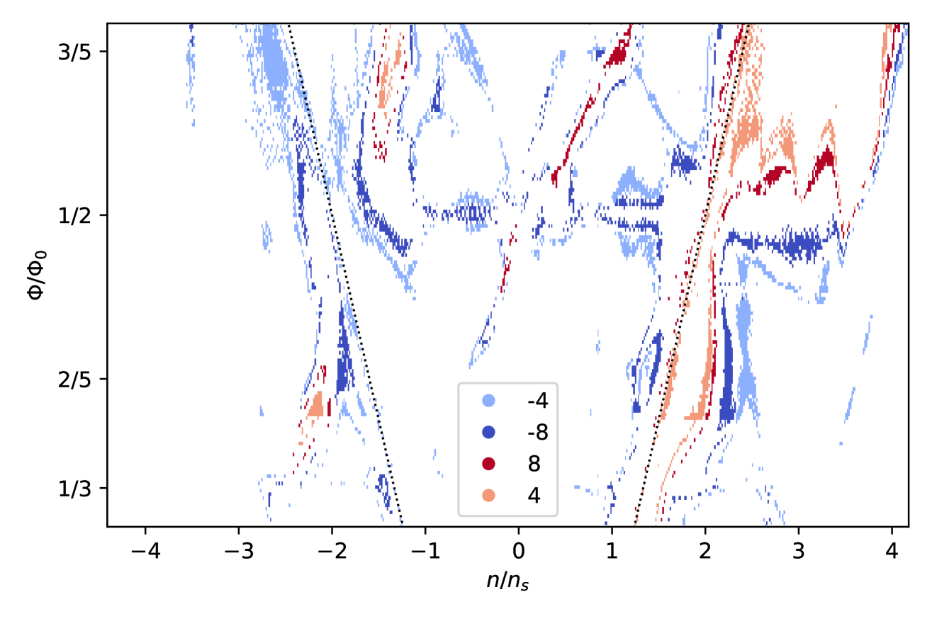
Figure S8: Integer quantum Hall plateaus. $\pm 200$ $\Omega$ windows for several different integer plateaus for contact pair 7 - 17. Dotted lines are (0, pm 4). Though the integer states are reasonably well quantized, they subtend far less of the Landau fan at these fluxes than 8/3.

We observe a bending Landau minifan emitting from $n/n_{s}=2,\Phi/\Phi_{0}=0.5$, where the $(0,\,4)$ Středa line intersects half-flux (Fig. 4). In longitudinal transport (panel A), the minifan pointing toward higher density and higher flux bends non-monotonically back toward half flux. Such bending is also visible in the minifan pointing toward lower flux, but in the following discussion we focus on the more prominent upward-pointing minifan. There is a small kink where the bending Landau minifan would have intersected the $(1,3)$ Středa line near $n/n_{s}=2.5$, and a complete reset at $n/n_{s}=3$. In Hall measurements (panel B), we observe $h/4e^{2}$ and $h/8e^{2}$ integer quantum Hall plateaus following the same bending behavior, including a third reset near $n/n_{s}=3.5$ (see also Fig. S8).

This reset behavior is not the same bending behavior noted in Ref. [36] and cannot be understood in a non-interacting model of rigid bands. It is reminiscent of the spontaneous flavor polarization at integer filling in magic-angle twisted graphene structures at zero field [2, 3, 47, 48]. However, though spontaneous polarization into an isospin flavor can lead to reset behavior, it does not explain the observation that a dip in longitudinal resistance coincident with quantized Hall resistance follows a nonlinear trajectory in the space of filling and flux; an incompressible Chern gap must follow the appropriate Středa relation.

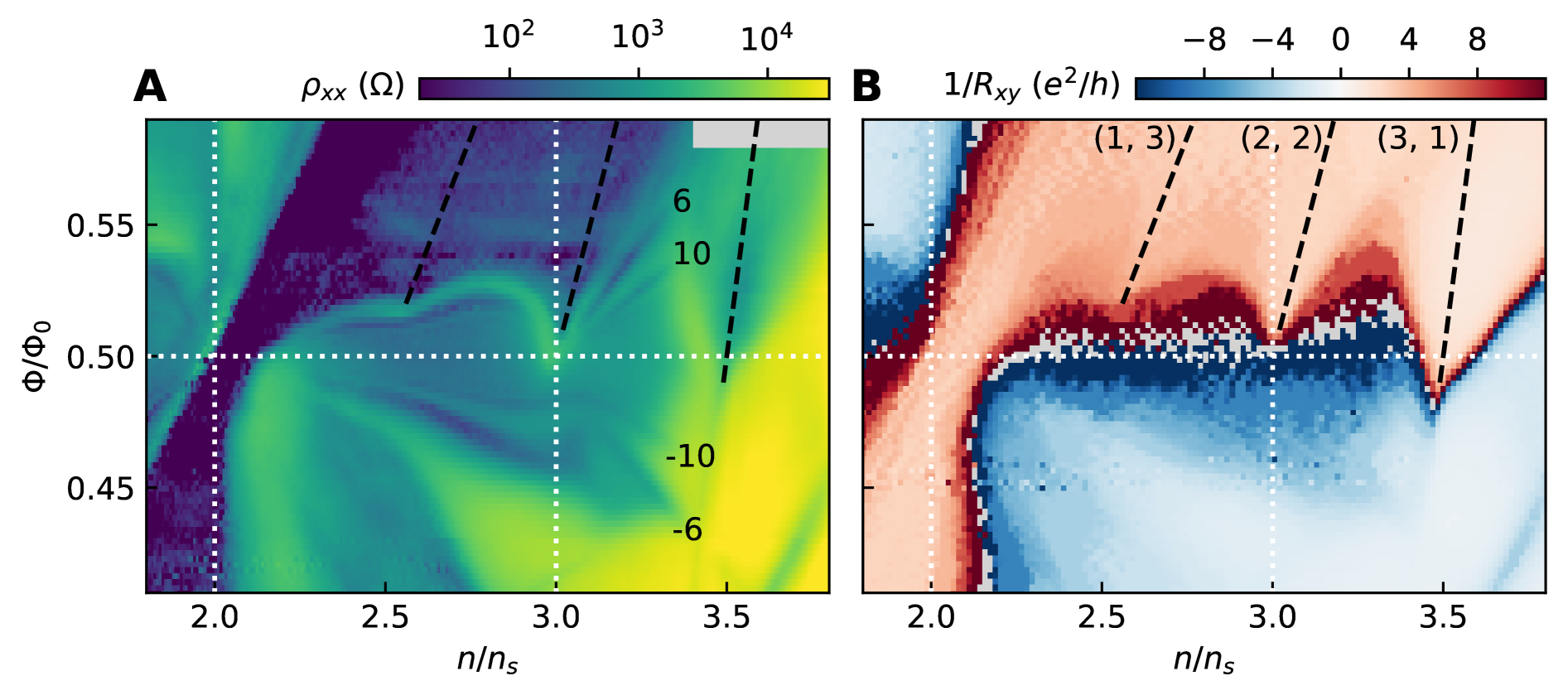
Figure 4: Landau level reset at half flux. (A) Zoomed segment of Fig. 1 showing the Landau levels bending and resetting at half flux. The numbers $\pm 6$ and $\pm 10$ are the slopes ($t$ values) of the faint lines $(3,\pm 6)_{1/2}$ and $(3,\pm 10)_{1/2}$ to their left. (B) Inverse Hall resistance showing that quantization of the Hall resistance tracks the bending dips in longitudinal resistance. Detail of all contact pairs in Figs. S10, S11, and S12.

For each of the four combinations of spin and valley, the two zero-field moiré minibands split into four magnetosubbands at half flux, reflecting a unit cell doubling in the Hofstadter spectrum. Because of this unit cell doubling, integer filling of the highest-energy magnetosubband (two valley-degenerate subbands split by Zeeman) corresponds to fillings $n/n_{s}=2.5$, $3$, $3.5$, and $4$ referenced to the original unit cell. At $n/n_{s}=3$, if the carriers within this band fully polarize into half of the available flavors, we expect a total Chern number of all filled bands of 2. One can see this from the fact that this gap must be the same as the (2, 2) Hofstadter subband ferromagnet state emanating from zero field [9, 24]. Landau levels emanating from half flux carry $C=2$, therefore we would expect a four-fold degenerate fan with an offset of 2 ($t=\pm 2,6,10,\ldots$) emanating from $n/n_{s}=3$. In our measurements, the Landau levels emanating from the reset point are indeed fourfold degenerate, with $(3,\pm 6)_{1/2}$ and $(3,\pm 10)_{1/2}$ being the only visible gaps. Here, we use the subscript $1/2$ to indicate we are using $s$ to reference a density offset at half of a flux quantum per moiré unit cell.

The resets do not all appear at exactly half flux. Rather, the reset seen in both longitudinal and Hall measurements near $n/n_{s}=2.5$ is just above half flux, and the reset seen in Hall at $n/n_{s}=3.5$ is just below half flux. Each reset aligns with an extrapolation of a Hofstadter ferromagnetic state—$(1,3)$, $(2,2)$, and $(3,1)$, respectively—from zero field (dashed lines).

V Discussion of possible mechanisms for extended FCI

We turn now to the $8/3$ fractional state which surprisingly persists over a larger range of density than any integer state. A $18.5$ T linecut near 2/5 flux (Fig. 2B, C) traverses the three largest pockets of quantization in the Landau fan diagram, centered at $n/n_{s}=-1.3,1.9$, and $2.6$. These occur upon doping into the next band above the Hofstadter gaps $(0,-4)$, $(0,+4)$, and $(+4,-4)$, respectively. Assuming the total Chern number $\pm 8/3$ extracted from measured Hall resistance is the sum of the Chern number $\Delta t$ of the FCI and that of the gapped integer state below, the Chern numbers of the three FCI states would be $4/3=-8/3-(-4)$, $-4/3=8/3-4$, and again $4/3=-8/3-(-4)$, respectively. In Fig. 3A, we mark with labels $\alpha$, $\beta$, and $\gamma$, respectively, the parent spin-polarized Hofstadter subbands at 2/5 flux within our single-particle model that we believe host the FCI states. If there is minimal mixing of bands from interactions, we are in each case doping into a spin-polarized (all blue in the figure) but valley-degenerate band. Thus the 4/3 Chern number referenced above could represent two copies of a $|\Delta t|=2/3$ FCI. It could instead be one copy of 4/3, or even four copies of 1/3 if we could recover a larger degeneracy.

Unlike ordinary Landau levels, the three subbands we postulate as parents for the FCIs have finite bandwidth, even without disorder. Subband $\gamma$ is the narrowest at $\sim 1$ meV. The others have width $\sim 2$ meV at 2/5 flux, and the associated FCIs extend over a range of flux for which the bands broaden further and even overlap with nearby subbands, factors we would ordinarily expect to disfavor formation of FCI states.

Specifically, subband $\alpha$ and its corresponding Hall plateau are enigmatic. We observe an enormous region of quantization ($\Delta n/n_{s}\sim 0.5$), larger than any other plateau—integer or fractional—between $0$ and $28$ T (see Fig. S8). An incompressible gap is expected to follow a well-defined Středa relation with slope equal to the total Chern number of the occupied bands. However, the breadth of this plateau stymies assigning a specific ($s$, $t$). To retain quantization as carrier density is tuned, the excess carriers must go into localized states. What states are doping into here? The obvious culprit would be localized states from disorder. While we cannot explicitly rule out disorder, it is unlikely that localized states from disorder would specifically extend these $\pm$8/3 fractional gaps so much more dramatically than other gaps in the spectrum. In Sec. S12 and Sec. S13, we discuss the effects of domain walls and spin-dependent transport, respectively. We consider both scenarios possible but unlikely as explanations of our data.

A more likely reason for these fractional plateaus to be so large is the formation of a fractional partial Hall crystal: a Wigner crystal in a FCI background. In this scenario, upon doping with respect to primitive filling of the FCI gap, the strongly-interacting dilute system of quasiparticles forms a Wigner crystal. As this crystal is topologically trivial, insulating, and compressible, it does not contribute to transport, so quantized Hall resistance is retained or restored at the value associated with the FCI state [40].

This mechanism has been invoked to explain reentrant quantum Hall in 2D electron gases [38, 39], but for the present system we have two complicating factors. First, the presence of a moiré potential might be expected to favor forming a Wigner crystal not at a continuous range of density but specifically at rational fractional fillings of the moiré. We instead observe sustained quantization over a range of density that would encompass many simple fractions. Second, this plateau occurs in a regime of two valley-degenerate Hofstadter subbands, with bandwidth comparable to Zeeman splitting. There could thus be more than one way for the multiple flavors to combine into a fractional state, reminiscent of $\nu=2/3$ fractional quantum Hall in a seminconductor double quantum well [49]. Understanding the nature of the extended FCIs and the conditions for a subband to fractionalize warrant further experimental and theoretical investigation. If the electronic solid picture we suggest is correct, disentangling the precise nature of the solid, including whether it is partially or entirely composed of a second flavor of the composite fermions themselves, will be an important challenge.

Acknowledgments We would like to thank Steve Kivelson, Julian May-Mann, Trithep Devakul, Yves Kwan, Tomohiro Soejima, Patrick Ledwith, Ben Feldman, Matt Yankowitz, Dave Cobden, Xiaodong Xu, Wei Pan, Jonah Herzog-Arbeitman, Nisarga Paul, and Sayak Bhattacharjee for fruitful discussions. Sample preparation, measurements, and analysis were supported by the US Department of Energy, Office of Science, Basic Energy Sciences, Materials Sciences and Engineering Division, under Contract DE-AC02-76SF00515. Device fabrication was performed at the Stanford Nano Shared Facilities which is supported by the NSF under award ECCS-2026822. D.G.-G. acknowledges support for supplies from the Ross M. Brown Family Foundation and from the Gordon and Betty Moore Foundation’s Emergent Phenomena in Quantum Systems (EPiQS) Initiative through grant GBMF9460. X.W. acknowledges financial support from National MagLab through Dirac fellowship, which is funded by the National Science Foundation (Grant No. DMR-1644779) and the state of Florida. O.V. was funded in part by the Gordon and Betty Moore Foundation’s EPiQS Initiative Grant GBMF11070 and acknowledges support from the National High Magnetic Field Laboratory funded by the National Science Foundation (Grant No. DMR-2128556) and the State of Florida. K.W. and T.T. acknowledge support from JSPS KAKENHI (Grant Numbers 19H05790, 20H00354 and 21H05233). Part of this work was performed at the Stanford Nano Shared Facilities (SNSF), supported by the National Science Foundation under award ECCS-2026822.

Supplemental material

S1 Generalized Diophantine and Definitions

For concreteness, we explicitly follow the terminology used in [40], which we reproduce here. For a number of carriers per unit area $\bar{\rho}$, we write a generalized Diophantine equation as

$$\bar{\rho}=\nu_{s}\rho_{\phi}+\eta_{s}A_{0}^{-1},$$ (1)

where $\nu_{s}$ and $\eta_{s}$ are rational numbers, $\rho_{\phi}$ is the density of flux quanta per unit area, and $A_{0}$ is the unit cell area associated with the spatially modulated (crystalline) electron density. The Hall conductance is given by

$$\sigma_{xy}=-\nu_{s}e^{2}/h.$$ (2)

Both an incompressible (fractional) quantum Hall liquid and a Hall crystal are described by the case where $\nu_{s}\neq 0$ and $\eta_{s}=0$. In the latter case, the system spontaneously breaks translation symmetry with density fluctuations set by $\rho_{\phi}$ while maintaining a non-zero Hall conductance. In an anomalous Hall crystal, time reversal symmetry breaks spontaneously in addition to translation symmetry breaking. A Wigner crystal, however, is described by $\nu_{s}=0$ and $\eta_{s}\neq 0$ and therefore must have vanishing Hall conductance.

A partial Hall crystal is, in some sense, an intermediate phase combining the properties of both. It is described by $\nu_{s}\neq 0$ and $\eta_{s}\neq 0$. Therefore, it will have a non-zero Hall conductance and spatially modulated electron density. Given the Wigner crystal background, a partial Hall crystal will be compressible if the spatial modulation of the electron density is not strongly pinned to a disorder potential.

S2 Transport measurements

We measured the sample in the SCM-32T system at the National High Magnetic Field Laboratory (MagLab). Although the hybrid magnet had a nominal maximum field of 32 T, because we were one of the early users of the system, we were restricted to a maximum field of 28 T. We used the top-loading dil fridge insert with a base temperature of 50 mK at the mixing chamber plate. The sample probe had 16 DC measurement wires, so we were not able to measure every contact pair in our device.

The probe did not feature cold low-pass filters. We included low-pass filters (borrowed from another user and described in Ref. [50]) at the breakout box, however there was still RF pickup between the breakout box and the sample. This was most evident at 8 PM every day, when a nearby radio station turned down their output power and our measurement noise decreased. For example, in Fig. 1, we crossed 16.8 T at 8 PM, where there is a noticable increase in sharpness of features.

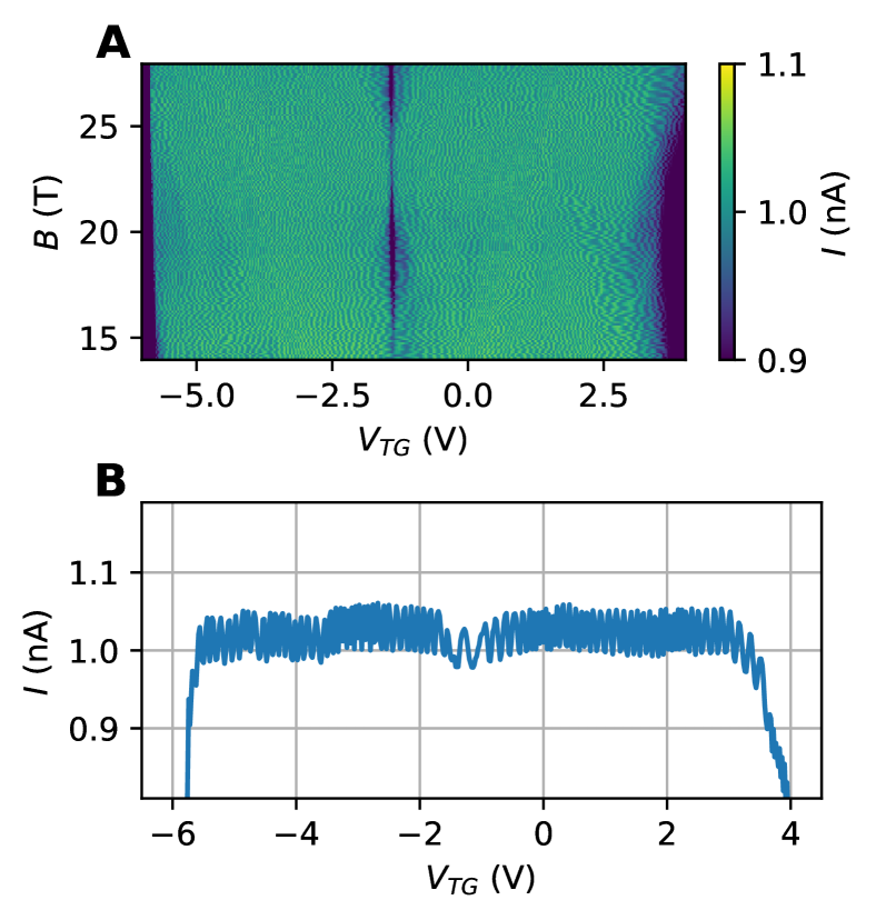
Figure S6: Current noise. (A) Current vs gate and field. (B) Line cut at $B=14$ T. Note that the average current is a few percent above 1 nA.

In addition to RF noise blurring our measurements, they also suffered from low-frequency noise within the measurement instruments themselves. This noise appeared in the current measurement for Fig. 2 (Fig. S6), but not in the associated voltage measurements for all densities/fields, meaning that the noise was not in the current itself. Thus, for Fig. 2, we do not use the current measurement, but instead divide by a constant 1 nA.

We sourced 1 nA of current at near 5 Hz using an SR860, sourcing one volt across a 1 G$\Omega$ resistor. We used SR550 and 560 voltage preamplifiers and SR830 and SR860 lock-in amplifiers to measure voltages. We used an Ithaco 1211 current preamplifier and an SR860 to measure current.

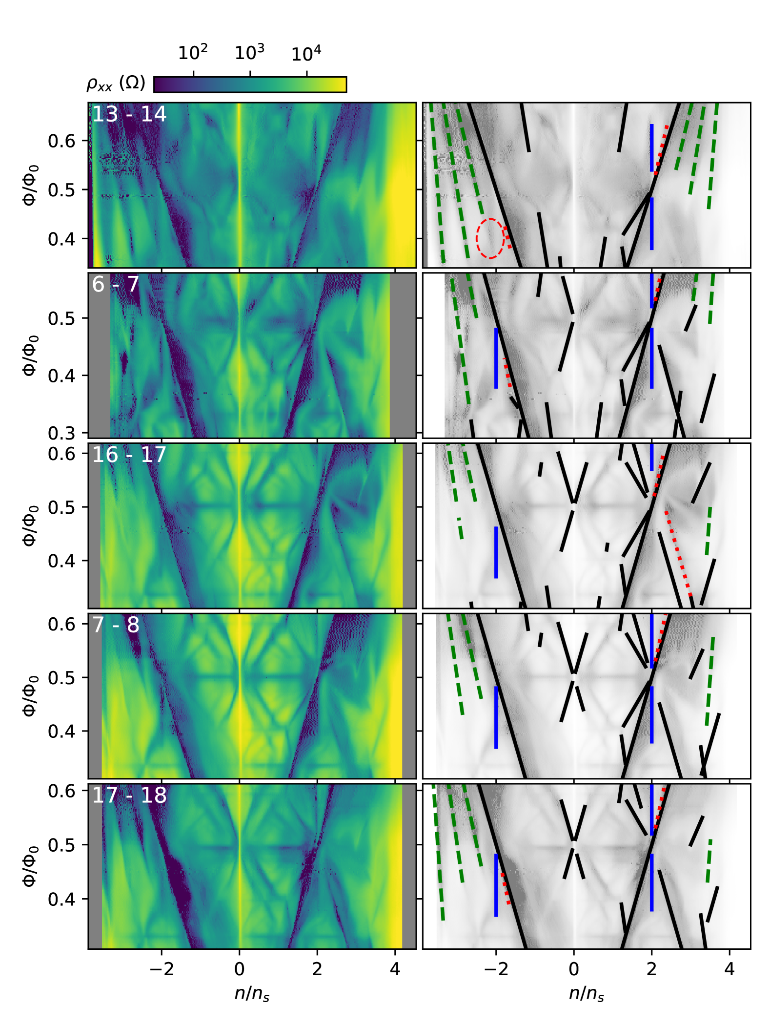
Figure S2: All longitudinal contact pairs. Measured separately from Fig. 1, which was a remeasurement of contact pair 7-8. (Left panels) The longitudinal resistivity of the indicated contact pairs. (Right panels) Corresponding schematic with the same interpretation as in Fig. S1B. The red circle for contact pair 13 - 14 indicates a feature that we could not unambiguously identify. It does not appear to be (-1, -3), which can be seen above it.

We took the first set of measurements on many contact pairs at once (Figs. S2 and S3). The Hall measurements in Fig. 2 were taken in this set. We then found that only measuring one contact pair at a time greatly reduced noise. We therefore took the measurement in Fig. 1, consisting only of a single longitudinal resistance measurement, separately.

We show a comparison between the data taken at MagLab with data taken in our own system at Stanford in Fig. S4. The system at Stanford both has a lower base temperature and high quality filters at the mixing chamber stage. There are two stages of filtering: the wires are first passed through a cured mixture of epoxy and bronze powder to filter GHz frequencies, then low-pass RC filters mounted on sapphire plates filter MHz frequencies. As a result, the Landau fan appears much sharper. The resistivity near charge neutrality is nearly an order of magnitude higher in our measurements at Stanford compared to those at MagLab.

There is one notable difference between how the measurements were performed at Stanford vs MagLab. At Stanford, our contacts became highly resistive when the graphite back gate was held at ground, so we fixed the graphite back gate to 1.5 V for the measurements. At MagLab, we found that the contacts were an order of magnitude lower resistance than what we saw at Stanford, so we left the graphite back gate at ground. The difference in contact resistances was likely a function of the higher effective temperature.

S3 Cluster filtering

The unfiltered data from Fig. 2 can be seen in Fig. S21. To filter the data, we begin by identifying points where the Hall resistance $R_{xy}$ falls within some window of our desired value ($\pm 1\%$ of $\pm 3h/8e^{2}$ in this case). Binary dilation is applied to the windowed data such that nearest-neighbors within this masked array are now included. Each contiguous cluster of the dilated data set is then identified, and, if it does not contain above a threshold number of points, the original undilated points are omitted from the final filtered data set. Because of the dilation and generous threshold, this filtering primarly serves to remove isolated data points with no next-nearest-neighbor point within the window.

S4 Brown-Zak oscillations

At rational values of $\Phi/\Phi_{0}=p/q$, the system can be described in terms of Bloch states in a $q$-times enlarged magnetic Brillouin zone [51, 52]. In transport, this manifests as oscillations in conductivity at simple field fractions and constant density. These “Brown-Zak” oscillations have been observed in graphene/hBN superlattices[53, 54, 55]. The homogeneity and amount of disorder in the sample affects the maximum $q$ for which oscillations will be visible, because as $q$ increases, the size of the magnetic Brillouin zone increases relative to the carrier mean free path [54].

We observe Brown-Zak oscillations at $\Phi/\Phi_{0}=1/3$, $2/5$, $1/2$, and $3/5$ (panel B, horizontal dotted lines). Of note, the Brown-Zak oscillations at $1/2$ flux appear only between $n/n_{s}=\pm 2$. The density-dependent amplitude of the oscillations is a probe of the carrier group velocity and therefore the miniband width [54]. So, where we do not see Brown-Zak oscillations, we should expect flatter bands and thus stronger electron correlations. In general, we observe more and stronger Brown-Zak oscillations on the electron side of charge neutrality compared to the hole side, consistent with the basic principle that the hole bands are flatter than electron bands in TBG.

We observe a similar set of Brown-Zak oscillations in contact pairs 16-17, 7-8, and 17-18 (Figs. 1 and S2). Contact pair 6-7 has generally blurrier features, and has broad oscillations only at $\Phi/\Phi_{0}=1/2$ and $1/3$. Contact pair 13-14 does not show clear oscillations, likely both because of inhomogeneity and also closer proximity to the magic angle.

It would be convenient if the Brown-Zak oscillations were ideally sharp features in field, because their broadening would be a function of twist angle inhomogeneity. Then, assuming Gaussian disorder (a likely wrong assumption), it would be straightforward to compute $\sigma_{\theta}$ from the FWHM of the BZ oscillations via

$$\sigma_{B}=\frac{4h\theta}{\sqrt{3}ea^{2}}\left(\Phi/\Phi_{0}\right)\sigma_{\theta}.$$

Unfortunately, in Fig. 1, the width of the oscillations in the oscillations is not set by twist angle inhomogeneity. This can be readily ascertained from the fact that the features at $\Phi/\Phi_{0}=3/5$ are significantly sharper than those at $1/2$.

Near $\Phi/\Phi_{0}=p/q$, the Bloch electrons feel an effective field [53]

$$B_{\mathrm{eff}}=B-\frac{\Phi_{0}}{A}\frac{p}{q}.$$

This is an aspect of Hofstadter’s butterfly’s fractal nature.

S5 Single-particle bends, SBCI, Hofstadter ferrogmagnetism

As demonstrated in Ref. [36], not all relatively straight lines in field/density with low resistance are Str̆eda gaps. Instead, relatively straight-line features of low resistivity can appear where one anisotropy-smeared butterfly spectrum is coincident with another. These false Str̆eda lines have a characteristic behavior at intersections with lines from the other doubled butterfly. Many of the features within our measurements follow the same pattern (see Fig. 3), and we attempt to only place lines in Fig. 1B where we are confident that there is a gap.

We observe a few Str̆eda lines with fractional $s=\pm 1/2$ and $t=\pm 3$ near half flux (red dotted lines in panel B). As they appear to emit from $n/n_{s}=\pm 2$ at half flux, we would describe them as $(\pm 2,\pm 3)_{1/2}$. Such lines have been described as symmetry-broken Chern insulators in the literature [19], and we observe at least one of them in all of the contact pairs that we measured. Curiously, in another contact pair, a symmetry-broken Str̆eda line $(13/3,-4)=(3,-4)_{1/3}=(7/3,-4)_{1/2}$ runs between one third and one half flux.

We observe states with $s+t=\pm 4$ projecting from integer $s$ (green dashed lines in Figs. 1 and S2). In all contact pairs, they tend to extend to lower field on the hole side compared to the electron side (Fig. S2). In samples from the literature near the magic angle, they extend to zero or near zero field [3, 56, 47, 22, 57, 7, 8, 9]. These lines are described theoretically as correlated Hofstadter ferromagnetic states in Ref. [42], meaning they have polarized spin and valley degrees of freedom of interaction-modified bands.

S6 Str̆eda line fit procedure

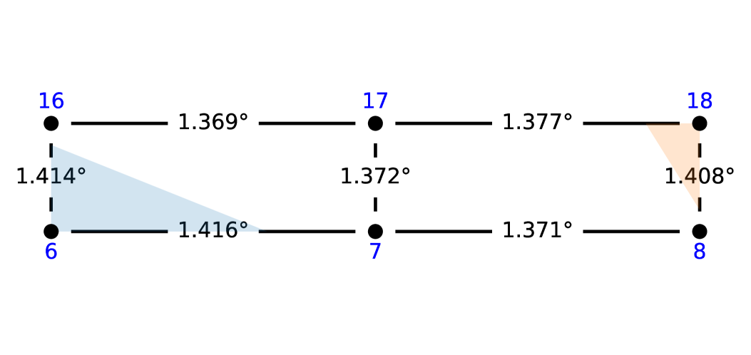
Figure S5: Twist angle variation. Blue-labelled points are our contacts. The pitch between contacts is 3 $\mu$m. The channel is 1 $\mu$m wide. Vertical lines between them are Hall pairs, and horizontal lines are longitudinal pairs. The estimated $\theta$ values for each contact pair (Table S1) are laid over the lines, with uncertainties elided for brevity. Shaded regions indicate our guess of regions with different twist angles, based on nearby twist angles and the sharpness of features in the measurements.

The raw data for Figs. 1, S2, and S3 are in gate-voltage vs magnetic field. We transform the data into $n/n_{s}$ vs $\Phi/\Phi_{0}$ by placing points along sharp lines with known $(s,t)$ by-eye. Brown-Zak oscillations additionally constrain $\Phi/\Phi_{0}$. We then use least squares to fit parameters $m_{g}$, $b_{g}$, and $B_{0}$, where $n/n_{s}=m_{g}V_{g}+b_{g}$ and $\Phi/\Phi_{0}=1$ at $B=B_{0}$. The resulting fit parameters are shown in Table S1 and schematically with our device geometry in Fig.S5. Quantum capacitance, owing to its dependence on density of states, precludes an accurate global conversion between gate voltage and density. The fits should be assumed to be at least a few percent wrong where the density of states is low.

After fitting the global conversion parameters to lines with known $(s,t)$, we were able to assign $(s,t)$ to the remaining straight-line features. Most of the lines could be easily assigned by-eye, and the results for all contact pairs are shown in Fig. S2. We note that not all relatively straight-line minima in $R_{xx}$ correspond to quantum Hall Str̆eda lines, as noted in Ref. [36]. We attempted to correctly label only Str̆eda lines in Figs. 1 and S2.

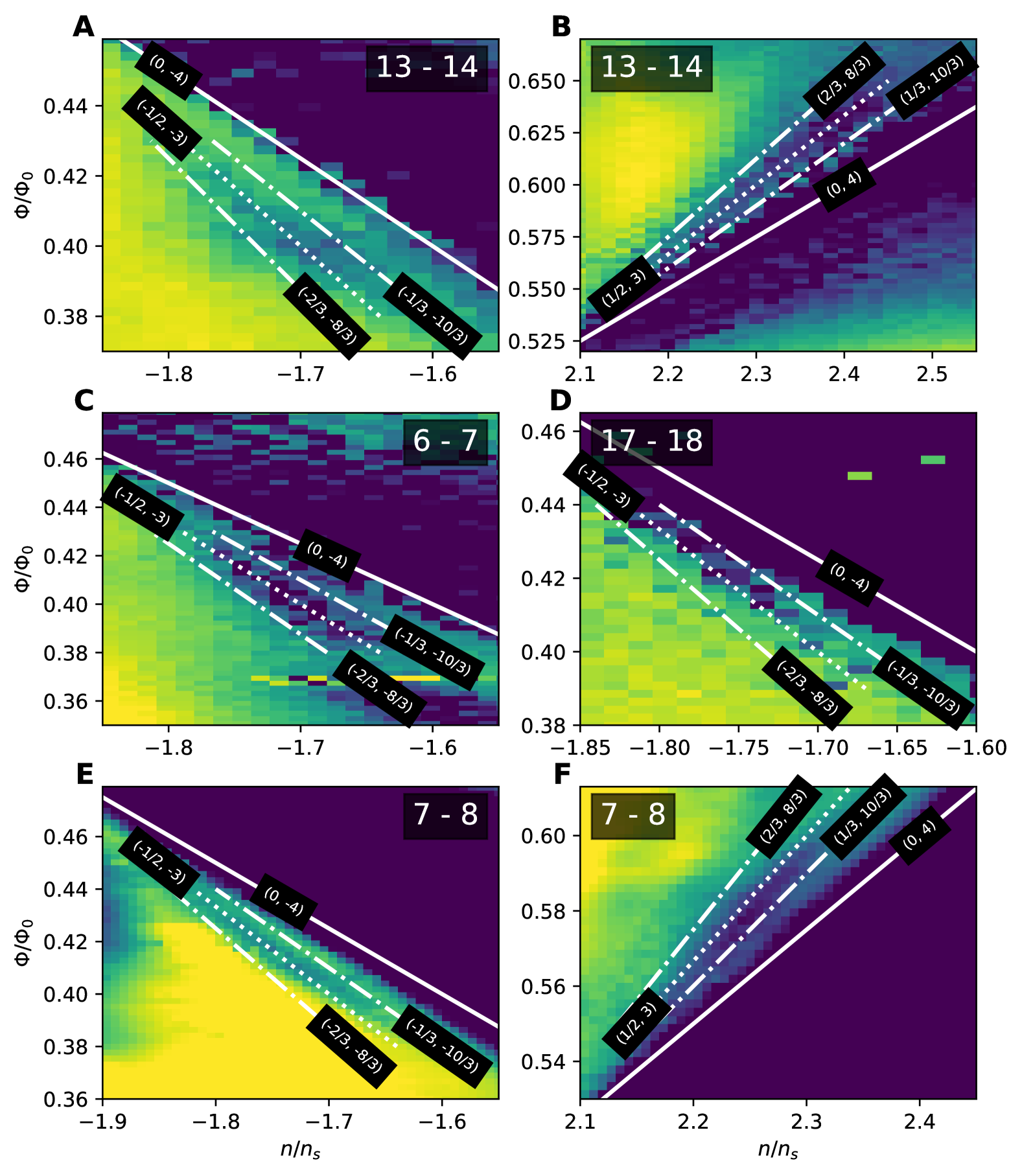
Figure S9: Fractional or symmetry-broken Str̆eda lines near half flux? Panels A-D are the same data as in Fig. S2. Panels E-F are the same data as in Fig. 1. Colormaps are adjusted for each panel to highlight the relevant line. Fits to $(\pm 1/2,\pm 3)$ (dotted lines) are better than fits to third fractions (dash dotted lines) in all cases except for panel F.

Because of the $8/3$ FCI states nearby, we expected to find Str̆eda lines with slope $8/3$ near half flux. As shown in Fig. S9, the candidate lines are actually better fit by $s=\pm 1/2$, $t=\pm 3$. These lines appear closely associated with half flux, so are better described by $(\pm 2,\pm 3)_{1/2}$.

	$m_{g}$ (V-1)	$b_{g}$	$B_{0}$ (T)	$A$ (nm2)	$\theta$ (°)
13 - 14	$0.843\pm 0.005$	$1.171\pm 0.009$	$41.2\pm 0.4$	$100.4\pm 0.9$	$1.309\pm 0.006$
6 - 16	$0.723\pm 0.003$	$1.023\pm 0.006$	$48.0\pm 0.3$	$86.1\pm 0.5$	$1.414\pm 0.004$
6 - 7	$0.716\pm 0.002$	$0.990\pm 0.005$	$48.2\pm 0.2$	$85.8\pm 0.3$	$1.416\pm 0.002$
16 - 17	$0.774\pm 0.002$	$1.082\pm 0.004$	$45.1\pm 0.1$	$91.7\pm 0.2$	$1.369\pm 0.002$
7 - 17	$0.772\pm 0.002$	$1.081\pm 0.004$	$45.2\pm 0.2$	$91.5\pm 0.3$	$1.372\pm 0.003$
7 - 8	$0.771\pm 0.002$	$1.093\pm 0.003$	$45.1\pm 0.1$	$91.8\pm 0.1$	$1.369\pm 0.001$
7 - 8*	$0.770\pm 0.001$	$1.085\pm 0.002$	$45.2\pm 0.1$	$91.6\pm 0.1$	$1.371\pm 0.001$
17 - 18	$0.769\pm 0.002$	$1.096\pm 0.004$	$45.6\pm 0.1$	$90.8\pm 0.3$	$1.377\pm 0.002$
8 - 18	$0.734\pm 0.007$	$1.041\pm 0.010$	$47.6\pm 0.7$	$86.8\pm 1.3$	$1.408\pm 0.011$

Table S1: Voltage to density conversion parameters. *: Fit to the data in Fig. 1. The rest of the rows are fits to the data in Fig. S2. It is important that $m_{g}$ and $B_{0}$ agree between the two measurements of contact pair 7 - 8, and they do. On the other hand, $b_{g}$ may vary over time as charge impurities and the like change. Areas and twist angles, along with their uncertainties, are calculated assuming zero strain. We know there is uniaxial heterostrain of order $0.2$% in this sample, so the uncertainty in $\theta$ is underestimated.

S7 Other contact pairs

Fig. S5 shows a schematic of the device with measured twist angles overlaid. We can make a rough estimate of which regions in the device have inhomogeneity/different twist angles based on the measured twist angles along with the sharpness of features. For instance, contact pairs 6 - 16 and 6 - 7 have both a higher measured twist angle but also show very blurry features in transport. Hence, we draw the blue region. Contact pairs 17 - 18 is slightly blurry, and has a slightly higher twist angle than its neighbors, but contact pair 8 - 18 is very blurry and has a significantly higher twist angle, hence the orange region. These regions are only our guesses.

Significant differences between neighboring contact pairs has the unfortunate consequence that analyses that rely on comparing two measurements, typically $R_{xy}$ and $\rho_{xx}$, are not trustworthy.

S8 Detail of Landau level reset

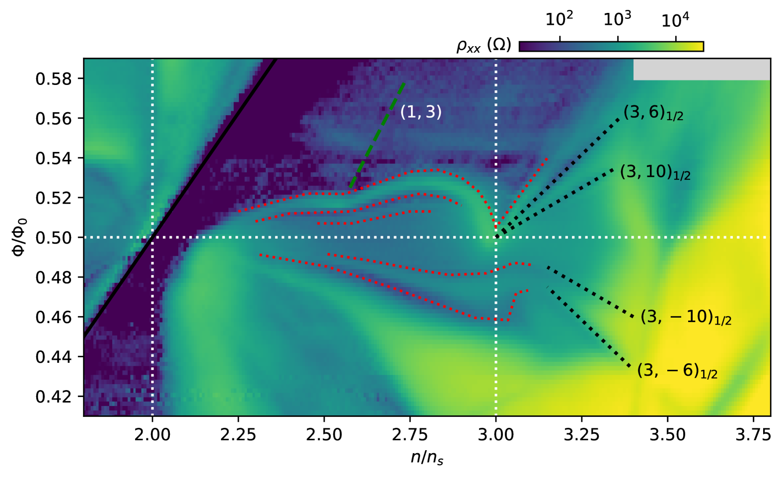
Figure S10: Detail of LL reset. Data from Fig. 1. Other contact pairs shown in Figs. S11 and S12. The green dashed line $(1,3)$ is not prominently visible in the resistivity, but lines up with the kink in the red dotted line below it. The red dotted lines indicate minima in $\rho_{\mathrm{XX}}$ and likely correspond to Landau level gaps. The black dotted lines are minima that follow the indicated paths

Figs. S10, S11, and S12 magnify the bending Landau minifan near $n/n_{s}=2$, $\Phi/\Phi_{0}=1/2$ from Figs. 1, S2, and S3.

In Fig. S10, red dotted lines mark bending, low-resistance states. The green dashed $(1,3)$ line is not visible as a minimum in $\rho_{xx}$. Instead, we include it to highlight that there is a kink in the red dotted lines where it would intersect them. This line corresponds to an integer filling $\nu=1$ of the band at half flux. After the reset at $n/n_{s}=3$ (half filling of the band, or $\nu=2$), we observe Str̆eda lines $(3,\pm 6)_{1/2}$ and $(3,\pm 10)_{1/2}$.

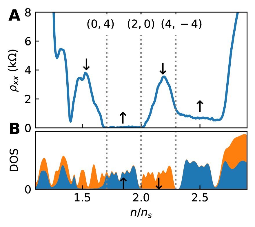
Figure S27: Possible spin-dependent transport. (A) Line cut from Fig. 1 along the dotted white line at 19.2 T. Intersections with the $(0,4)$, $(2,0)$, and $(4,-4)$ Hofstadter gaps are indicated with vertical dotted lines. (B) Density of states at $p/q=19/45$ ($B\approx 19.1$ T). Spin up and down states are indicated in blue and orange respectively, as well as with arrows in both panels.

The fourfold LL degeneracy is consistent with fully polarizing half of the bands at half flux. We note that above the topmost dotted red line, the transport behavior is the same as the spin-up regions described in the main text and Fig. S27. We suspect, therefore, that the band at half flux has fully spin-polarized at $n/n_{s}=3$.

S9 Vertical lines

In Fig. 3A, a dashed ellipse is drawn which encircles three sets of bands: one narrow red band near -343 meV, and two broader sets of bands between -330 and -320 meV. The narrow red band carries a Chern number of -4 and a net spin down, while the two broadened bands each carry a Chern number of 2 and have opposite spins. Thus, if the Fermi level is set within the gap on the left side of the ellipse, there is no net Chern number: $-4+2+2=0$. However, there is a net spin: the broadened band’s spins cancel each other, but there is no spin to cancel the narrow red band’s spin. This net property will hold even if the higher-energy bands are modified by interactions. All four gaps with this property are marked with Xs in panels A and B.

This situation is reminiscent of a quantum spin Hall insulator. We might expect, therefore, quantized longitudinal along with zero transverse resistance. In our longitudinal measurements, we tend to see vertical lines of minimal resistivity, often below our measurement floor of roughly 1 Ohm, however in many cases the minima is higher. Unfortunately, because of measurement noise and differences between neighboring contact pairs, our measurements are insufficient to make strong claims about the transport properties of these states.

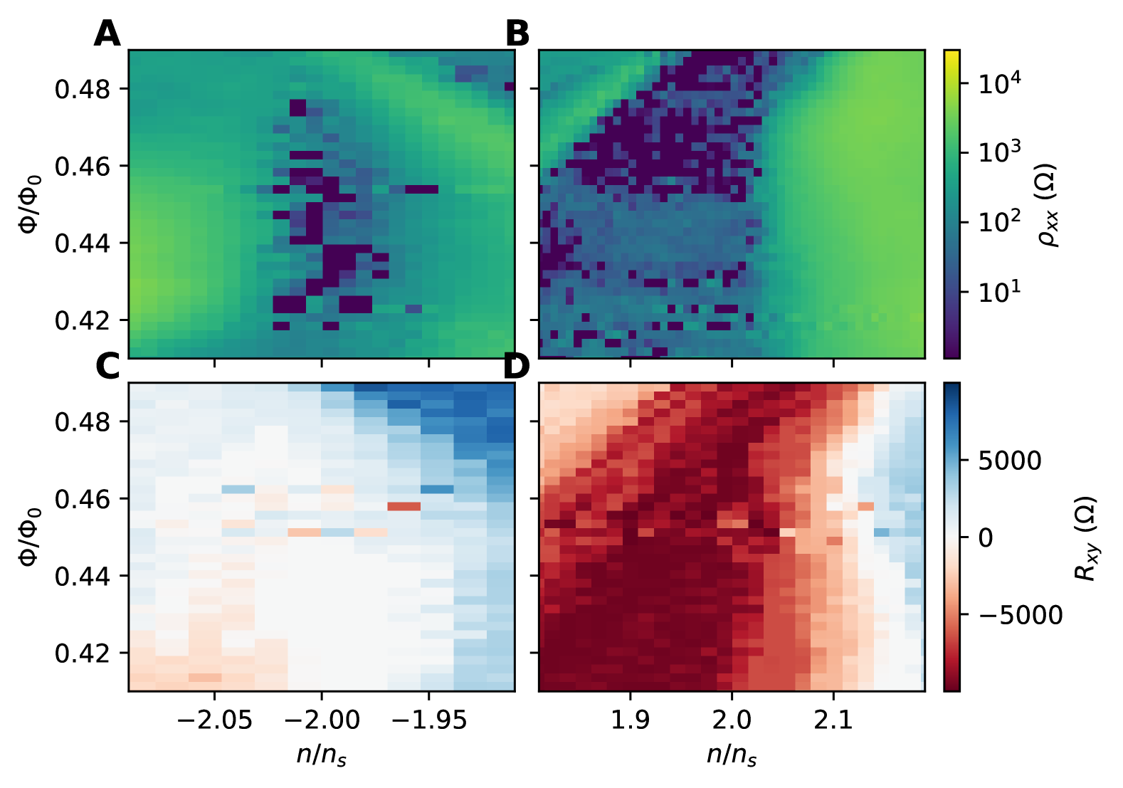
Figure S13: Fine detail of potential QSH. (A-B) Zoom in on Fig. 1 near the clear vertical-line features. (C-D) Same, for contact pair 7 - 17.

Fig. S13 shows zoom-in regions just below half flux near $n/n_{s}=\pm 2$ for the high-quality fan in Fig. 1 and the good Hall pair from Fig. 2. At $n/n_{s}=-2$, $\rho_{xx}$ drops below our measurement floor of roughly 1 Ohm (panel A), and the Hall resistance is zero (panel C). At $n/n_{s}=2$, there is a vertical-line transition from low to high resistance rather than an isolated minimum (panel B), and the Hall resistance is not zero (panel D). Zero longitudinal and Hall resistance simultaneously would be some exotic superconducting state, but we do not claim to have such a state here. Rather, we expect our measurements are a result of inhomogeneity within the device.

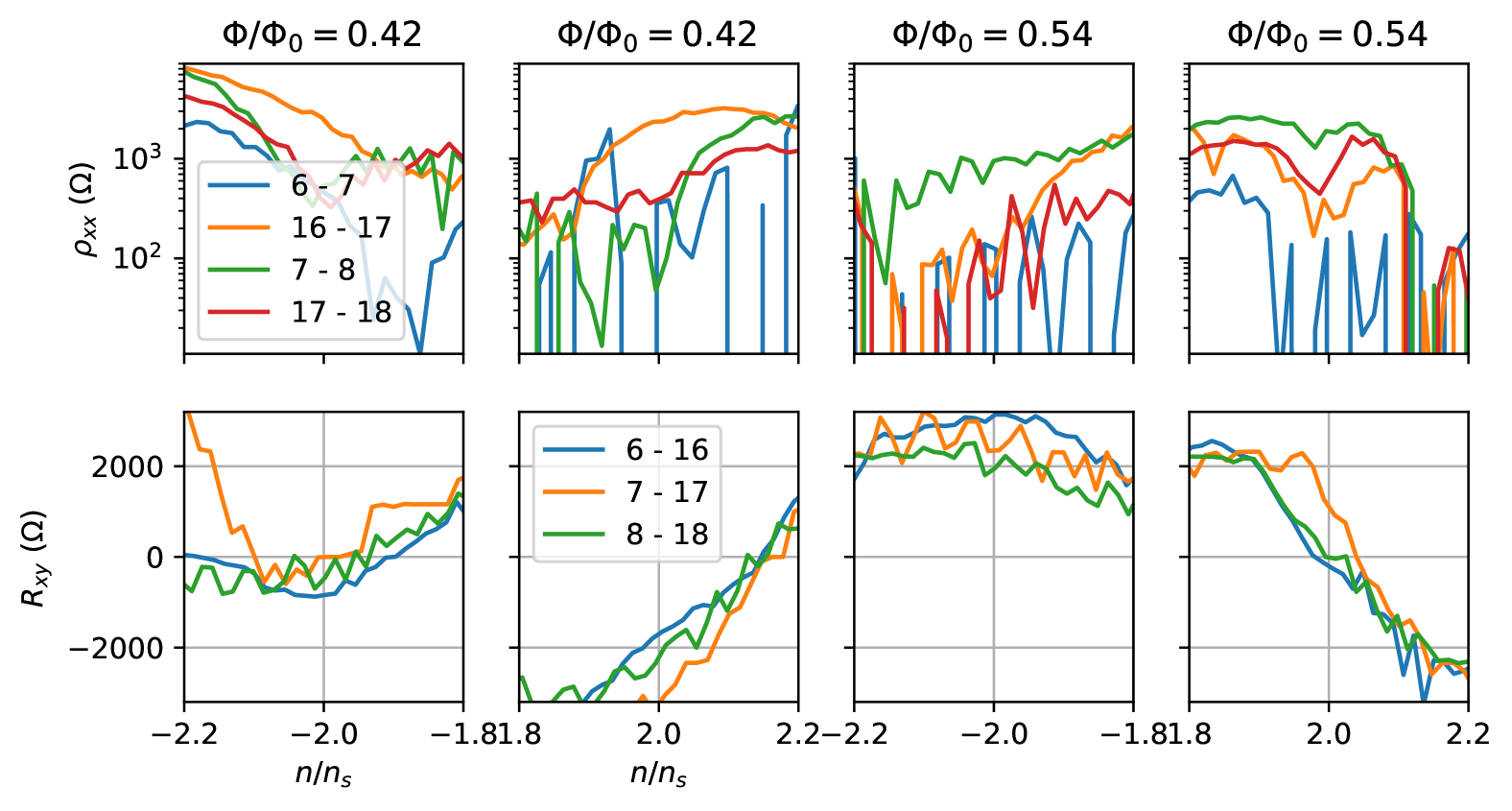
Figure S14: Line cuts near potential QSH. Top row: line cuts of longitudinal measurements (Fig. S2) at the indicated fields. Although there are some minima at $n/n_{s}=\pm 2$, there is too much noise in most measurements to clearly claim a certain behavior. Bottom row: ditto, but for Hall measurements (Fig. S3). Only contact pair 7 - 17 shows a clear plateau at zero resistance at $n/n_{s}=-2$ and $\Phi/\Phi_{0}=0.42$.

Many of the other longitudinal contact pairs show minima in resistivity, some dropping below our measurement floor of 1 Ohm (Fig. S2). However, from one contact pair to the next, these minima vary by orders of magnitude. The top row of Fig. S14 shows $\rho_{xx}$ for all contact pairs near the four locations with vertical lines. The cuts are noisy and mostly unimpressive. Only contact pair 7 - 17 (the good pair with FCI) shows a clear zero resistance plateau at $n/n_{s}=-2$.

S10 How well quantized is the Hall resistance?

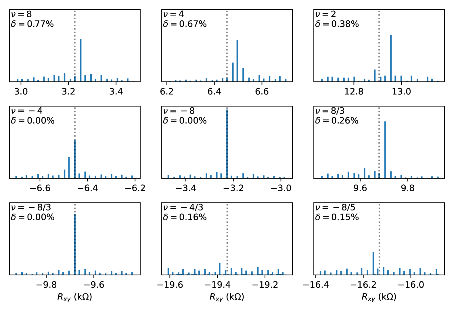
Figure S15: How well quantized is the Hall resistance? Each panel shows a histogram (over the entire gate and field ranges) of $R_{xy}$ centered around the expected value of $h/\nu e^{2}$ (vertical dotted line) for $g=1.0785$ along with the computed $\delta$ value.

Fig. S15 shows histograms of $R_{xy}=V_{xy}/(1~\mathrm{nA})/g$ near the indicated $\nu$ values. Quantum Hall plateaus show up as sharp peaks in this histogram. The free parameter $g$ represents inaccuracies in the gains of our amplifier and current source, which we did not measure carefully at MagLab. Then, we compute a metric of quantization

$$\delta=\frac{\mathrm{argmax}_{R}-R^{*}}{R^{*}}$$ (3)

for each $\nu$ value. This metric is simple and does not consider, for instance, shoulders in the histogram. We show values of $\delta$ computed for $g=1.0785$. This number places $\nu=-8$, our most prominent quantum Hall plateau, directly on the expected value. It is instead possible to fine-tune $g$ to $1.0824$ so that all $\delta$ values are below 0.3%. Either way, we are confident in stating that our fractions are quantized to better than 1%. Note that 1.08 is a little high compared to our experience: typically the voltage pre-amps that we use at Stanford are only miscalibrated by a few percent. The 1.08 number also includes a factor from our current source, which we expect to be 1 to 2 percent based on the average of our noisy current (Fig. S6).

The simple $\delta$ metric does not consider the finite resolution of the voltage measurements: note that the histogram bins are typically spaced by a few tens of ohms. Assuming that it is $\sigma_{xy}$ that is quantized with

$$\sigma_{xy}=\frac{\nu e^{2}}{h}=\frac{R_{xy}}{R_{xy}^{2}+\rho_{xx}^{2}},$$ (4)

it is natural to ask how high can $\rho_{xx}$ be for $R_{xy}$ to still fall within the same histogram bin. For $\nu=\pm 8/3$, the bins are roughly 20 $\Omega$ wide, yielding $|\rho_{xx}|\lesssim 300\;\Omega$. Indeed, in many of the places that $R_{xy}$ is precisely quantized to $\pm 8/3$, $\rho_{xx}$ is of order a hundred ohms or less.

S11 Discussion of other fractions

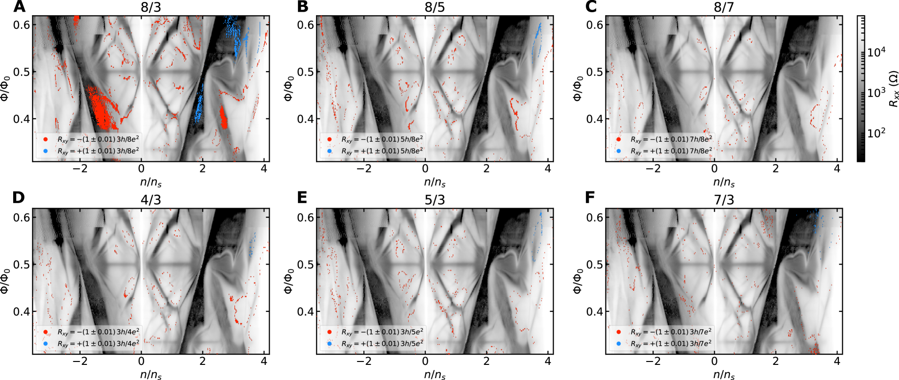
Figure S23: Highlighting values of Fractional Hall resistance In a similar manner to Fig. 2A of the main text, the longitudinal resistance is shown in grey-scale. We then highlight regions where the Hall resistance falls within 1% of the specified fractional value: A $\pm 8/3$ (reproduced from main text), B $\pm 8/5$, C $\pm 8/7$, D $4/3$, E $5/3$, and F 7/3. Our clustering algorithm has been applied to remove spurious points (see Sec. S3).

In a similar manner to Fig. 2, in Fig. S23 we highlight where the Hall resistance $R_{xy}$ falls within a 1% window about a specified fraction. We see that $\pm 8/3$ is substantially more robust than the other displayed fractions. Most notably, $\-8/5$ and $-4/3$ exhibit the largest regions of quantization. Fractions not shown do not exhibit sizable regions that fall within a 1% window.

S12 Modeling a domain wall

To model the effects of a domain wall between two different Chern insulating regions with Chern numbers $C_{l}$ and $C_{r}$, we can use the Landauer-Büttiker formalism,

$$I_{i}=\frac{e^{2}}{h}\sum_{j}(\bar{T}_{ji}V_{j}-\bar{T}_{ij}V_{i}),$$ (5)

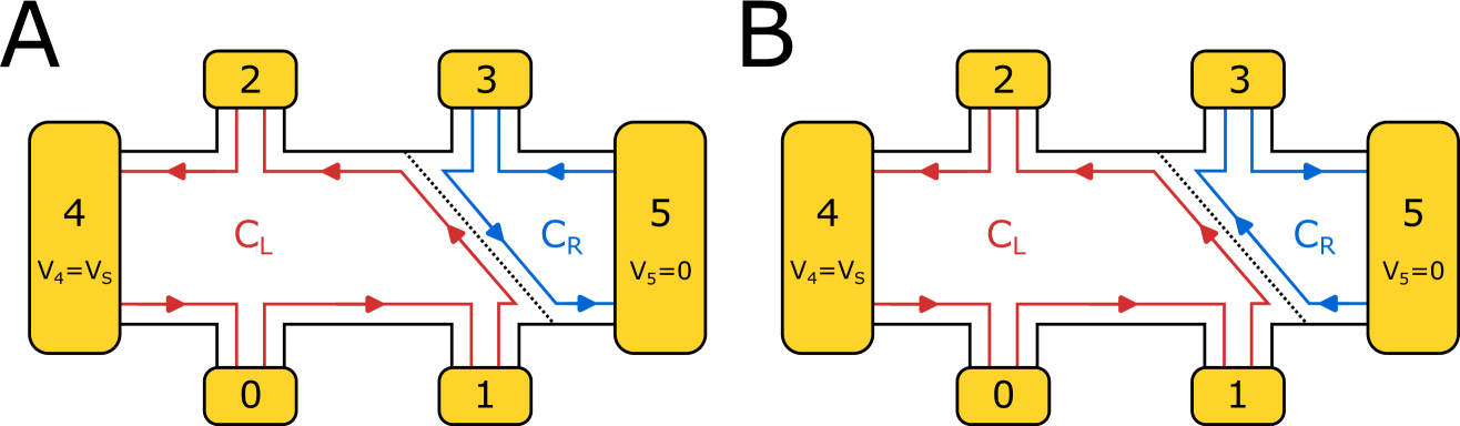
Figure S16: Hall bar with a domain wall. Schematic diagram of a Hall bar with a domain wall between two Chern insulating regions with different Chern number $C_{l}$ and $C_{r}$ for the case of when (A) $\mathrm{sgn}(C_{l})=\mathrm{sgn}(C_{r})$ and (B) $\mathrm{sgn}(C_{l})\neq\mathrm{sgn}(C_{r})$.

where the transmission coefficient $\bar{T}_{ij}=M_{ij}T_{ij}$ is the product of the number of modes $M_{ij}$ between contact j to contact i, and the transmittance $0\leq T_{ij}\leq 1$. We will consider the case of perfect edge modes with some probability $t$ of a carrier initially starting in one edge mode ending in another. This will only have meaningful consequence for modes at the domain wall, where the carrier can end up in the adjacent domain. Let us first consider the case of a domain wall which passes in-between a Hall pair with $\mathrm{sgn}(C_{l})=\mathrm{sgn}(C_{r})$ (Fig. S16A). Assuming the source contact 4 is at voltage V and the drain contact 5 is at 0, for such a configuration, the full system of equations is

$$\begin{pmatrix}m_{l}&0&0&0&-m_{l}&0\\ -m_{l}&m_{l}&0&0&0&0\\ 0&-\bar{T}_{12}&m_{l}&-\bar{T}_{32}&0&0\\ 0&0&0&m_{r}&0&-m_{r}\\ 0&0&-m_{l}&0&m_{l}&0\\ 0&-\bar{T}_{15}&0&-\bar{T}_{35}&0&m_{r}\end{pmatrix}\times\begin{pmatrix}V\\ V\\ V_{2}\\ 0\\ V\\ 0\end{pmatrix}=\begin{pmatrix}0\\ 0\\ 0\\ 0\\ I\\ -I\end{pmatrix},$$

where $m_{i}=|C_{i}|$. Then

$$V_{2} =T_{12}V,$$

$$I =m_{l}V(1-T_{12})=\bar{T}_{15}V.$$

We can then solve for the expected resistance values:

$$R_{xx}^{\mathrm{bot}} =\frac{V_{0}-V_{1}}{I}=0$$

$$R_{xx}^{\mathrm{top}} =\frac{V_{2}-V_{3}}{I}=\frac{T_{12}}{m_{l}}\frac{1}{1-T_{12}}$$

$$R_{yx}^{\mathrm{left}} =\frac{V_{0}-V_{2}}{I}=\frac{1}{m_{l}}$$

$$R_{yx}^{\mathrm{right}} =\frac{V_{1}-V_{3}}{I}=\frac{1}{m_{l}}\frac{1}{1-T_{12}}.$$

We can similarly consider the case of a domain wall which passes in-between a Hall pair with $\mathrm{sgn}(C_{l})\neq\mathrm{sgn}(C_{r})$ (Fig. S16B). Again, assuming the source contact 4 is at voltage V and the drain contact 5 is at 0, for such a configuration, the full system of equations is

$$\begin{pmatrix}m_{l}&0&0&0&-m_{l}&0\\ -m_{l}&m_{l}&0&0&0&0\\ 0&-\bar{T}_{12}&m_{l}&0&0&-\bar{T}_{52}\\ 0&-\bar{T}_{13}&0&m_{r}&0&-\bar{T}_{53}\\ 0&0&-m_{l}&0&m_{l}&0\\ 0&0&0&-m_{r}&0&m_{r}\end{pmatrix}\times\begin{pmatrix}V\\ V\\ V_{2}\\ V_{3}\\ V\\ 0\end{pmatrix}=\begin{pmatrix}0\\ 0\\ 0\\ 0\\ I\\ -I\end{pmatrix}.$$

For this case,

$$V_{2} =T_{12}V,$$

$$V_{3} =T_{13}V,$$

$$I =m_{l}V(1-T_{12}).$$

Solving for the expected resistance values:

$$R_{xx}^{\mathrm{bot}} =\frac{V_{0}-V_{1}}{I}=0$$

$$R_{xx}^{\mathrm{top}} =\frac{V_{2}-V_{3}}{I}=\frac{1}{m_{l}}\frac{T_{12}-T_{13}}{1-T_{12}}$$

$$R_{yx}^{\mathrm{left}} =\frac{V_{0}-V_{2}}{I}=\frac{1}{m_{l}}$$

$$R_{yx}^{\mathrm{right}} =\frac{V_{1}-V_{3}}{I}=\frac{1}{m_{l}}\frac{1-T_{13}}{1-T_{12}}=\frac{1}{m_{l}}\frac{T_{12}}{1-T_{12}}.$$

For either case, it would be possible to achieve a measured Hall resistance of 3/8 with the appropriate values of $m_{l}$ and $T_{12}$. However, such a scenario would yield markedly different values for $R_{xx}^{\mathrm{bot}}$ and $R_{xx}^{\mathrm{top}}$, which is inconsistent with our data. Therefore, we think such a domain wall in our sample is not the case.

Following this same procedure, one can see that a domain wall that does not pass between a Hall pair cannot yield a fractionally quantized Hall conductance.

S13 Spin dependent transport detail

There is a curious asymmetry in the longitudinal transport measurements. Observe the value of the resistivity on either side of $(0,\pm 4)$ in Fig. 1. On the left side (lower density), the resistivity tends to be in the kilohms, and there are numerous Str̆eda lines immediately next to the $(0,\pm 4)$ line (See Sec. S13 for more detail). On the right side (higher density), the resistivity tends to be lower than a kiloohm, and in some cases it is below one Ohm. In these regions, there are no Str̆eda lines, and the resistivity is flat and featureless.

As an example, the line cut along the white dotted line in Fig. 1 is shown in Fig. S27 panel A. To the left of $(0,4)$, the resistivity is peaks around 4 kilohms. To the right, between $(0,4)$ and $(2,0)$, it is only a hundred Ohms or lower. In panel B we show that these two types of transport correspond to states in the model that are entirely spin-polarized. Where the states are spin-up, we see low resistivity, and where they are spin-down we see high resistivity. Where we see a mixture of both, the resistivity is even higher. This behavior is followed in our measurements not just near $(0,\pm 4)$, but also in other regimes where the model reasonably matches the experiment. The major exception to this rule is near charge neutrality, where no substantial asymmetry is apparent.

Curiously, we only see FCI states in these low-resistivity (spin-up) regions. Circles in Fig. 3 panels A and B indicate regions where we observe $\pm 8/3$ FCI states. All of these regions are within blue Chern bands in panel A.

Spin-dependent resistivity has been observed in quantum Hall systems previously [58, 59, 60]. With Zeeman splitting, the lower-energy, spin-up states are filled first. Spin-down electrons then see a different magnetic environment: there is a substantial background of spin-up electrons already present. In high-quality WSe₂, this leads to the minority-spin resistance being dramatically increased at low temperatures [60]. We observe the same behavior here, however we are not confident that the underlying explanation is the same. We may be able to reverse the direction of resistivity with back gate voltage. We wish to emphasize that we do not have positive evidence for the hypothesis of spin-dependent transport.

S14 Continuum Model and Quantum metric

In this subsection, we discuss the Hamiltonian of the continuum model in the presence of both heterostrain and out-of-plane magnetic field. Heterostrain is described by a $2\times 2$ symmetric matrix $S_{\epsilon}$ which can always be diagonalized by an orthogonal matrix $R(\phi)$,

$$S_{\epsilon} =R_{\varphi}^{T}\begin{pmatrix}-\epsilon_{\mathrm{uni}}+\epsilon_{\mathrm{bi}}&0\\ 0&\nu\epsilon_{\mathrm{uni}}+\epsilon_{\mathrm{bi}}\end{pmatrix}R_{\varphi}\ .$$ (6)

where $R_{\varphi}=\begin{pmatrix}\cos\varphi&-\sin\varphi\\ \sin\varphi&\cos\varphi\end{pmatrix}$ is the two-dimensional rotational matrix with the angle of $\varphi$ that determines the two principal axes of the strain matrix $S_{\epsilon}$, and $R_{\varphi}^{T}$ is the transpose of the matrix $R_{\varphi}$, $\nu=0.16$ is the Poisson ratio as used in Ref. [37], and $\epsilon_{\mathrm{uni}}$ and $\epsilon_{\mathrm{bi}}$ are the uniaxial strain and biaxial strain respectively. In principle, the two layers may have different strain matrices $S_{\epsilon}^{(t)}$ and $S_{\epsilon}^{(b)}$, where the superscript $t$ and $b$ refers to top and bottom layers respectively. However, in this work, we consider only heterostrain with $S_{\epsilon}=S_{\epsilon}^{(t)}-S_{\epsilon}^{(b)}$ and neglect the homostrain $\frac{1}{2}(S_{\epsilon}^{(t)}+S_{\epsilon}^{(b)})$, since the shape of moire unit cell, the narrow band structure, the associated band properties, etc. are more sensitive to heterostrain whose impact is estimated as the maximal value of $\epsilon/\theta$ with $\epsilon=max(|\epsilon_{uni}|,|\epsilon_{bi}|)$ is the larger one between the uniaxial strain and the biaxial strain. On the other hand, the impact of homostrain is estimated as $\sim\epsilon$, much smaller than the heterostrain, and therefore can be safely neglected for small twist angles.

The impact of heterostrain on the non-interacting Hamiltonian have been discussed in Ref. [37, 43, 44], so we only briefly summarize the results in this manuscript. Following the model introduced in Ref. [43, 44], we recalculated the lattice relaxation in the presence of the heterostrain by iteration method. We found that the change of the relaxation by the applied heterostrain is the order of $\epsilon/\theta$. To achieve the precision of $1$ meV in the dispersion of the narrow bands and include the particle-hole breaking terms, our continuum model contains all the terms up to the second order in the gradient expansion, with all the parameters numerically calculated from the microscopic tight binding model proposed in Ref. [43, 44]. The Hamiltonian can be divided into two parts, the intralayer Hamiltonian $H_{\text{intra}}$ and the interlayer tunneling $H_{\text{inter}}$. The presence of heterostrain introduced several additional terms in $H_{\text{intra}}$. In addition to the coupling between the pseudo-scalar field induced by lattice distortion and the fermion density, $H_{\text{intra}}$ also includes the couplings between various strain-induced fields and the stress-energy of the Dirac fermion. $H_{\text{inter}}$ includes both the contact and gradient couplings. Since the tunneling constants, such as $w_{0}$, $w_{1}$, and $w_{2}$ in BM model, depends on both the microscopic interlayer hopping and the in-plane lattice distortion, and thus also depends on the applied strain. We have numerically calculated these coefficients with their values presented in Ref. [44, 61].

As illustrated in Ref. [37], the presence of heterostrain, in general, breaks the three-fold rotation $C_{3}$ and $C_{2x}$ symmetry, but still conserves $C_{2}\mathcal{T}$. As a consequence, the two Dirac cones around the CNP are not gapped, but the Dirac points are shifted to other momenta in the moiré Brillouin zone, and the two Dirac points are not degenerate anymore, with the energy difference manipulated by heterostrain and observable by quantum oscillation experiments.

Crucially, the three degenerate van Hove points become non-degenerate as uniaxial heterostrain is introduced. In Ref. [37], we measured the density of these non-degenerate van Hove points for both electrons and holes. Our model was electron/hole symmetric, so we could not fit to all six van Hove points simultaneously. Here, given we have now incorporated e-hole asymmetry, we can.

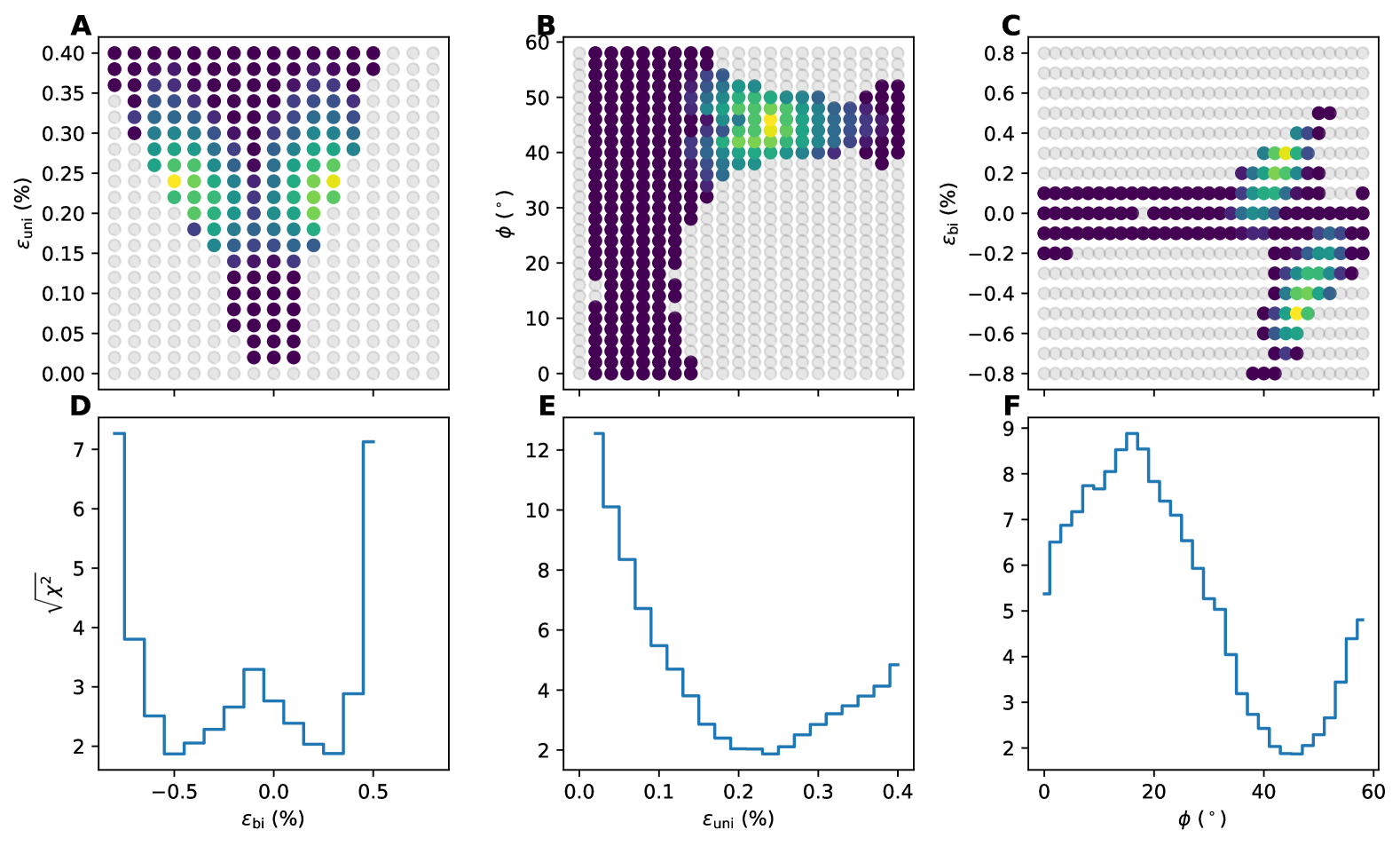
Figure S19: Best fit to low-field van Hove points. (A-C) $\chi^{2}$ metric for the two indicated parameters (yellow is low, purple is high), using the best value of the not shown third dimension. (D-F) One dimensions $chi^{2}$ metric, using the best value of both not shown dimensions.

Fig. S19 shows the $\chi^{2}$ statistic for a wide variety of moire parameters $\epsilon_{\mathrm{uni}}$, $\epsilon_{\mathrm{bi}}$, and $\phi$. Given these three free parameters, we choose $\theta$ such that the moire unit cell area is fixed. In practice, fixing $\theta$ instead to 1.37° does not make a significant change to these results.

There are two minima in $\epsilon_{\mathrm{bi}}$, at -0.5% and 0.3%. These two minima correspond to the same Hamiltonian after accounting for symmetries, with their asymmetry about zero $\epsilon_{\mathrm{bi}}$ coming from the Poisson ratio (which converts uniaxial heterostrain into both uniaxial heterostrain and a small amount of biaxial heterostrain). Thus, there is a unique set of parameters yielding a best fit.

In Ref. [37], we estimated an uncertainty of roughly $\delta\nu=\pm 0.05$ on each van Hove point. Here, our best-fit result does satisfy this bound on each van Hove point.

We hesitate to place uncertainties on our best-fit parameters, because we believe that they will be dominated by systematics. The model is not perfect, and it is not straightforward to account for model uncertainty. The uncertainties that we do report are based on the width of the minima in Fig. S19, and are underestimates.

The Hamiltonian in the presence of a magnetic field can be obtained by substituting the operator $\hat{\boldsymbol{p}}\longrightarrow\hat{\boldsymbol{p}}+e\boldsymbol{A}(\boldsymbol{x})$, with the Landau gauge $\boldsymbol{A}=B(0,y)$.

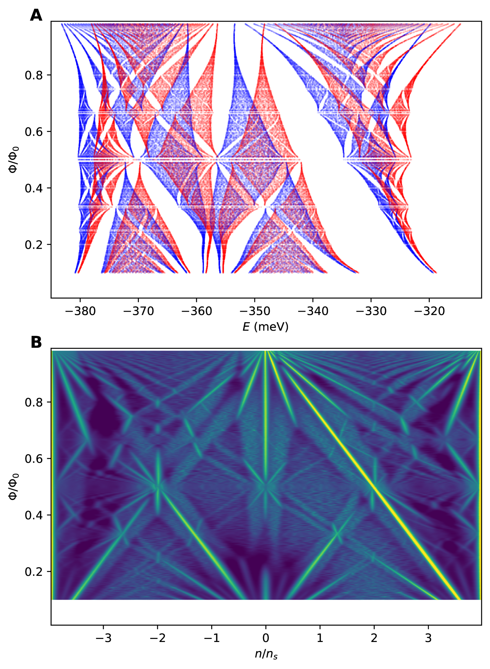
Figure S20: Hofstadter’s butterfly of the strained BM model. (A) Computed spectrum for $\theta=1.38^{\circ}$, uniaxial heterostrain $\epsilon=0.2$% at 0°angle, and $g=2$. Red means spin down, blue means spin up. (B) Computed inverse density of states.

For each field $p/q$, the computation produces a list of energies, eigenvalues of some large Hamiltonian. The number of energies produced is not the same from one field to another, growing with $q$. We then add a Zeeman term $E=\pm g\mu_{B}B/2$ for $g=2$ and $\mu_{B}$ is the Bohr magneton. Fig. S20A shows the resulting spectrum.

To convert the list of energies at a given field $E_{i}$ into something that we can plot versus density, we follow Ref. [62] and write

$$\rho(E)=\sum_{i}\frac{1}{\pi}\frac{\gamma}{(E-E_{i})^{2}+\gamma^{2}},$$

$$n(E)=\sum_{i}\frac{1}{\pi}\mathrm{arctan}\left(\frac{E-E_{i}}{\gamma}\right).$$

To normalize, divide each equation by the number of energies. The smoothing parameter $\gamma$ is not based on any temperature or disorder model. Fig. S20B is then $1/\rho(E)$ plotted against $n(E)$ and field. It is refreshing to see that even with such a simple model, much of the behavior from both Ref. [36] and the present manuscript are captured.

At the end of this subsection, we briefly review the definition of Berry connection and quantum metric for the Bloch states. As usual, the overlap of two Bloch states are

$$\langle u(\boldsymbol{k})|u(\boldsymbol{k}+\delta\boldsymbol{k})\rangle=1+\delta k_{\mu}\langle u(\boldsymbol{k})|\partial_{\mu}u(\boldsymbol{k})\rangle$$

$$+\frac{1}{2}\delta k_{\mu}\delta k_{\nu}\langle u(\boldsymbol{k})|\partial_{\mu}\partial_{\nu}u(\boldsymbol{k})\rangle+O(\delta k^{3})$$ (7)

where $u(\boldsymbol{k})$ is the perodic part of the corresponding Bloch state, i.e. $u(\boldsymbol{k})=e^{-i\boldsymbol{k}\cdot\boldsymbol{r}}\phi(\boldsymbol{k})$, where $\phi(\boldsymbol{k})$ is the Bloch state with the crystal momentum of $\boldsymbol{k}$. Here, the overlap $\langle u(\boldsymbol{k}+\delta\boldsymbol{k})|u(\boldsymbol{k})\rangle$ is expanded to the quadratic order of $\delta\boldsymbol{k}$. It is obvious that the linear part of $\delta k_{\mu}$ is proportional to the Berry connection, defined as

$$\mathcal{A}_{\mu}=i\langle u(\boldsymbol{k})|\partial_{\mu}u(\boldsymbol{k})\rangle$$

and can be shown to be real. Additionally,

$$\quad\langle u(\boldsymbol{k})|\partial_{\mu}\partial_{\nu}u(\boldsymbol{k})\rangle=-i\big{(}\partial_{\mu}\mathcal{A}_{\nu}+\partial_{\nu}\mathcal{A}_{\mu}\big{)}+\langle\partial_{\mu}\partial_{\nu}u(\boldsymbol{k})|u(\boldsymbol{k})\rangle\ .$$ (8)

Therefore, the imaginary part of $\langle u(\boldsymbol{k})|\partial_{\mu}\partial_{\nu}u(\boldsymbol{k})\rangle$ is

$$-\frac{1}{2}\big{(}\partial_{\mu}\mathcal{A}_{\nu}+\partial_{\nu}\mathcal{A}_{\mu}\big{)}$$ (9)

However, it does not appear in the quadratic terms of the expansion since it is an anti-symmetric tensor. We introduce the symmetric tensor $\gamma_{\mu\nu}$ for the real part

$$\gamma_{\mu\nu}=-\text{Re}(\langle u(\boldsymbol{k})|\partial_{\mu}\partial_{\nu}u(\boldsymbol{k})\rangle)$$ (10)

Thus, Eq. 7 can be rewritten as

$$\quad\langle u(\boldsymbol{k})|u(\boldsymbol{k}+\delta\boldsymbol{k})\rangle=1-i\mathcal{A}_{\mu}\delta k_{\mu}$$

$$-\frac{1}{2}\delta k_{\mu}\delta k_{\nu}\left(\gamma_{\mu\nu}+\frac{i}{2}\big{(}\partial_{\mu}\mathcal{A}_{\nu}+\partial_{\nu}\mathcal{A}_{\mu}\big{)}\right)+O(\delta k^{3})$$ (11)

However, the $\gamma$ tensor is $U(1)$ gauge dependent. To obtain a gauge-independent tensor, consider

$$\quad\left|\langle u(\boldsymbol{k})|u(\boldsymbol{k}+\delta\boldsymbol{k})\rangle\right|^{2}$$

$$=1-\delta k_{\mu}\delta k_{\nu}\left(\gamma_{\mu\nu}-\mathcal{A}_{\mu}\mathcal{A}_{\nu}\right)+O(\delta k^{3})$$ (12)

and thus, the quantum metric tensor is defined as

$$g_{\mu\nu}(\boldsymbol{k})=\gamma_{\mu\nu}(\boldsymbol{k})-\mathcal{A}_{\mu}\mathcal{A}_{\nu}$$ (13)

$$\Longrightarrow 1-\left|\langle u(\boldsymbol{k})|u(\boldsymbol{k}+\delta\boldsymbol{k})\rangle\right|^{2}=\delta k_{\mu}\delta k_{\nu}g_{\mu\nu}(\boldsymbol{k})+O(\delta k^{3})$$ (14)

In the presence of magnetic fields, the magnetic Bloch states might be written as the linear combination of Landau wave function instead of plane waves. In this case, the overlap between $u(\boldsymbol{k})$ and $u(\boldsymbol{k}+\delta\boldsymbol{k})$ is calculated as

$$\langle u(\boldsymbol{k})|u(\boldsymbol{k}+\delta\boldsymbol{k})\rangle$$

$$=\frac{1}{S_{\text{uc}}}\int_{\text{muc}}{\rm d}^{2}\boldsymbol{r}\ \phi^{*}_{\boldsymbol{k}}(\boldsymbol{r})e^{-i\delta\boldsymbol{k}\cdot\boldsymbol{r}}\phi_{\boldsymbol{k}+\delta\boldsymbol{k}}(\boldsymbol{r})$$ (15)

where $\int_{\text{muc}}{\rm d}^{2}\boldsymbol{r}$ integrates only over one magnetic unit cell, and $\phi_{\boldsymbol{k}}$ is the magnetic Bloch state with the magnetic momentum of $\boldsymbol{k}$. All these formula will be discussed in detail in Ref.[61].

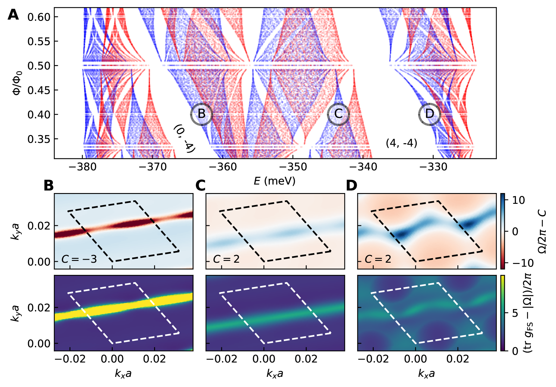
Figure S25: Computed Hofstadter spectrum and quantum geometric tensor. (A) Computed energy levels for $\theta=1.35^{\circ}$ with $0.24\%$ uniaxial heterostrain at 45° and $0.3\%$ biaxial heterostrain ($q\leq 72$), as described in the text. Spin up electrons are shown in blue, and spin down electrons are shown in red. The gaps at $(s,t)=(0,-4)$ and $(4,-4)$ are labeled. See Fig. S20 for the full range of fields. (B-D) Berry curvature (top panels) and trace condition (bottom panels) for the three labeled bands at 2/5 flux in panel A in the first moiré Brillouin zone. The black dashed lines correspond to the magnetic BZ. These three bands host the $-8/3$, $+8/3$, and $-8/3$ FCI states within the line cuts in Fig. 2, respectively. The trace and Berry curvatures are dimensionless, having been scaled by the area of the magnetic BZ. The units are not scaled to a unit cell area of $\sqrt{3}\pi^{2}/2\approx 8.5$

We show the Berry curvature and the trace of the quantum metric tensor for the bands featuring $\pm 8/3$ FCIs at 2/5 flux in Fig. S25. We note that the “trace condition” [63] is violated strongly in the case of one of these bands (panel B).

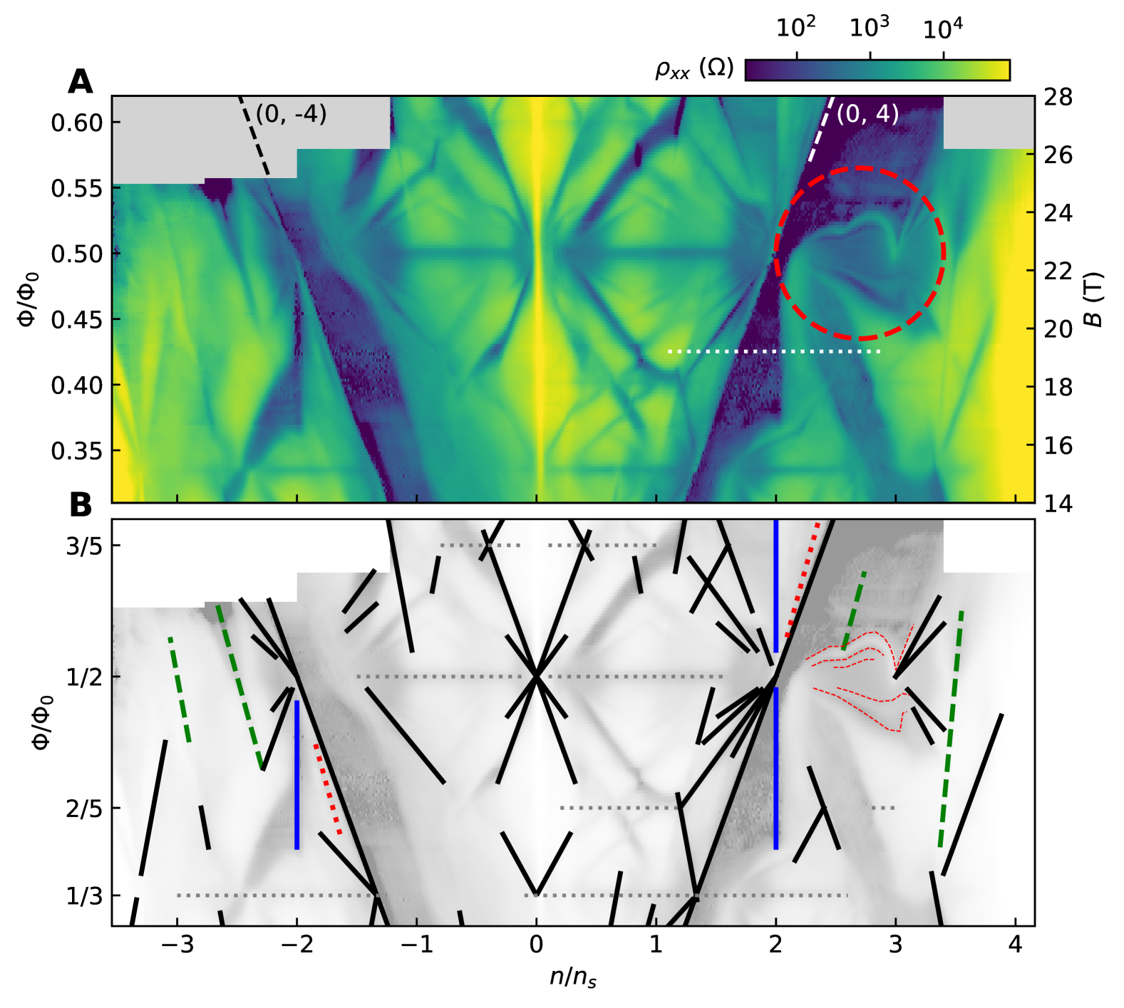
Figure S1: Longitudinal fan with schematic. (A) Same data as in Fig. 1. (B) Black lines are ordinary integer quantum Hall. Blue vertical lines are potential QSH sites (Sec. S9). Green dashed lines are correlated Hofstadter ferromagnetic states (Sec. S5). Red dotted lines are symmetry-broken Chern insulating states (Sec. S5). Red dashed lines are the bending Landau levels discussed in Sec. IV. Gray dashed lines are Brown-Zak oscillations.

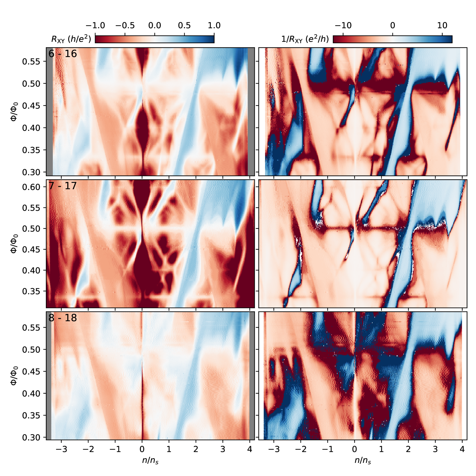
Figure S3: All Hall contact pairs. (Left panels) $R_{\mathrm{xy}}$ for the indicated contact pairs. (Right panels) Corresponding $1/R_{\mathrm{xy}}$. Line cuts for each are shown in Fig. S7. Note that contact pairs 6 - 16 and 8 - 18 show significantly blurrier features compared to 7 - 17.

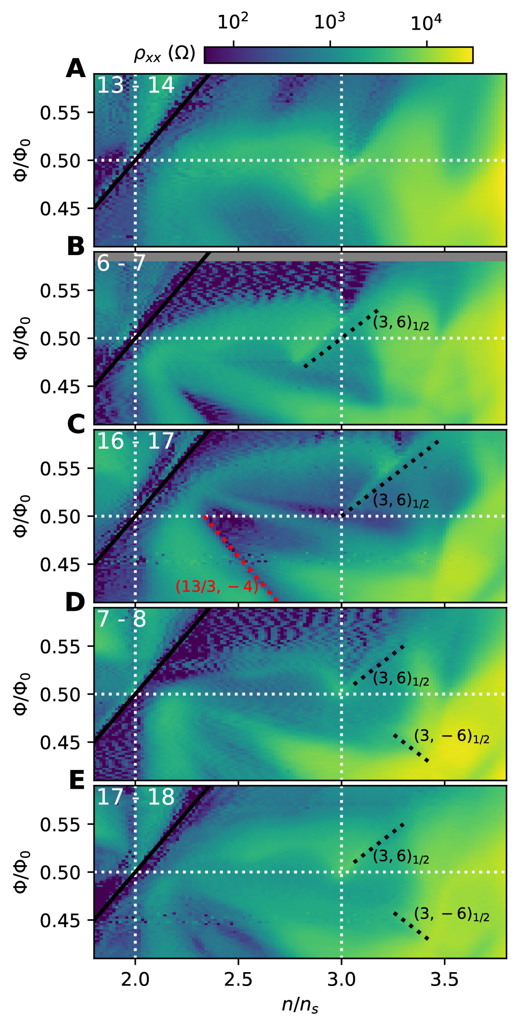
Figure S11: Detail of LL reset, continued. All longitudinal contact pairs, labelled as in Fig. S10.

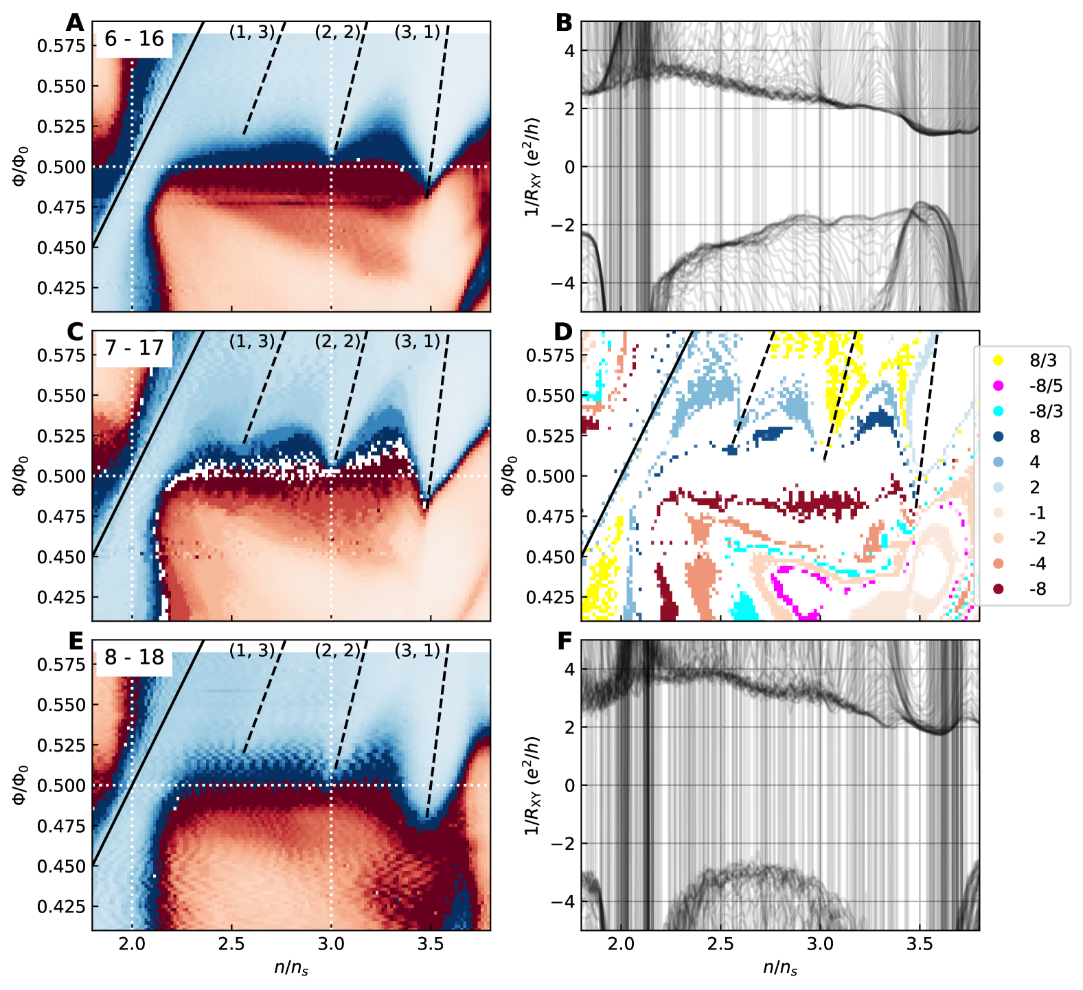
Figure S12: Detail of LL reset, continued. All three Hall contact pairs show a change of sign near half flux (ACE). There appear to be features associated with the Str̆eda lines $(1,3)$, $(2,2)$, and $(3,1)$, however the Hall conductivity never has the expected value for them (BDF). The sign change along the $(2,2)$ line happens very close to half flux and $n/n_{s}=3$, however the sign change along $(3,1)$ happens slightly below half flux in all cases.

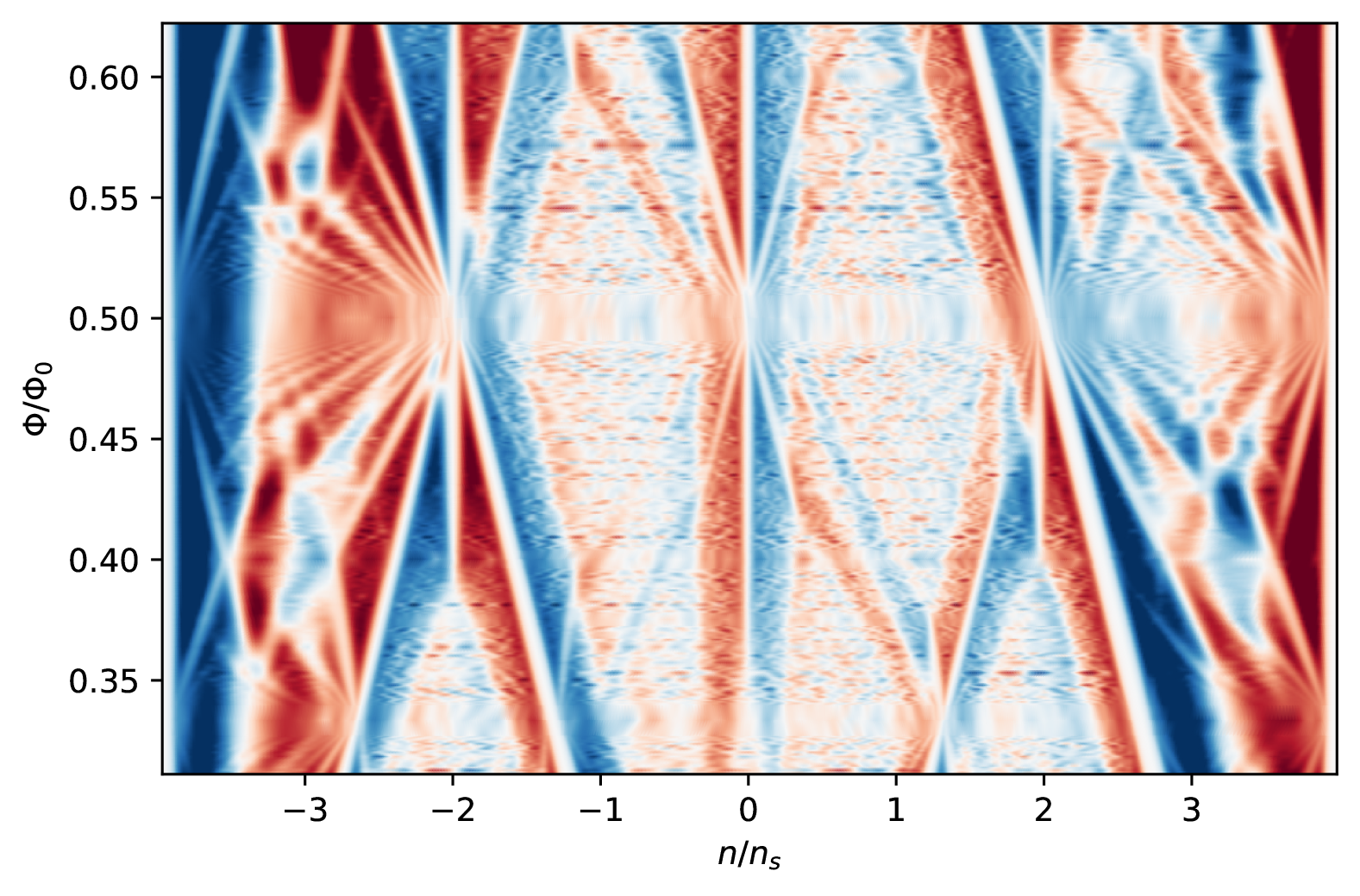
Figure S17: Spin states in computation. Density of states for spin up minus spin down. Blue means more spin-up than spin down, and red is the opposite.

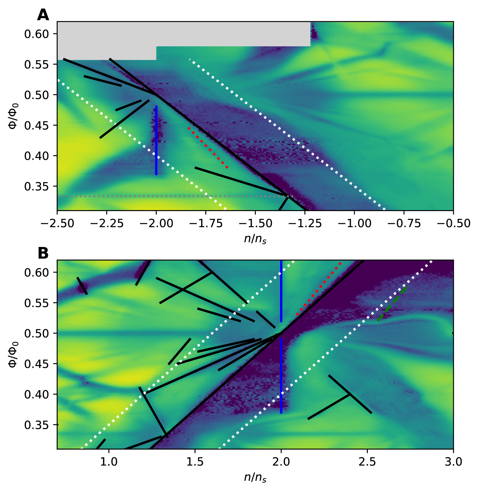
Figure S18: Spin-dependent transport detail. Zoomed in from Fig. 1. On the left side of $(0,-4)$ (A) and $(0,4)$ (B), the resistance is higher than on the right side and there are Str̆eda lines (black lines). Dotted white lines approximate where we start to have two spin species. See Fig. S17.

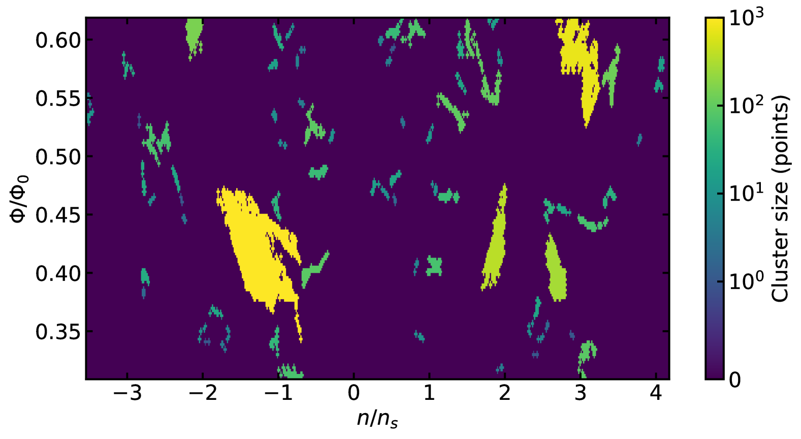
Figure S22: Clustering mask for $\pm 8/3$. Here we color code clusters by the number of points included in the cluster. Nearest neighbors and next-nearest neighbors that both fall within the defined window will be included in a cluster.

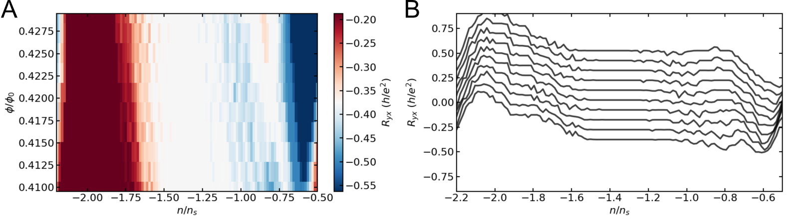
Figure S24: Possible reentrant FCI. (A) Zoomed in colorplot of the Hall resistance in on the largest plateau of -8/3 quantization. Colorbar is centered about $3h/8e^{2}$, such that white regions are well quantized. (B) Waterfall plot of (A) with curves offset for clarity. There is a loss of quantization roughly around -1 $n/n_{s}$ with quantization recovered on either side.

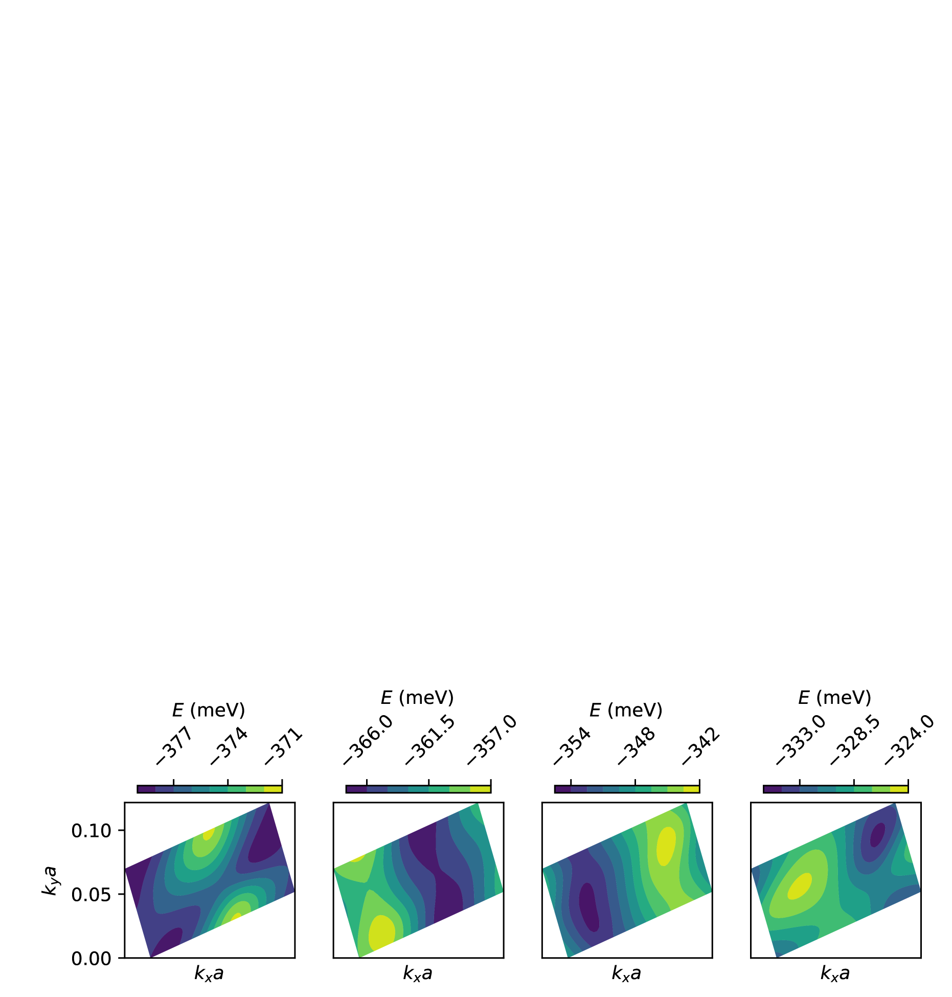
Figure S26: Computed band structure at 1/2 flux. Computed energy levels for the four bands at half flux. The middlemost bands have regions of open orbits.

References

- [1] Cao, Y. et al. Correlated insulator behaviour at half-filling in magic-angle graphene superlattices. Nature 556, 80–84 (2018). URL http://dx.doi.org/10.1038/nature26154.
- [2] Cao, Y. et al. Unconventional superconductivity in magic-angle graphene superlattices. Nature 556, 43–50 (2018). URL http://dx.doi.org/10.1038/nature26160.
- [3] Yankowitz, M. et al. Tuning superconductivity in twisted bilayer graphene. Science 363, 1059–1064 (2019). URL http://dx.doi.org/10.1126/science.aav1910.
- [4] Sharpe, A. L. et al. Emergent ferromagnetism near three-quarters filling in twisted bilayer graphene. Science 365, 605–608 (2019). URL http://dx.doi.org/10.1126/science.aaw3780.
- [5] Andrei, E. Y. & MacDonald, A. H. Graphene bilayers with a twist. Nature Materials 19, 1265–1275 (2020). URL http://dx.doi.org/10.1038/s41563-020-00840-0.
- [6] Balents, L., Dean, C. R., Efetov, D. K. & Young, A. F. Superconductivity and strong correlations in moiré flat bands. Nature Physics 16, 725–733 (2020). URL http://dx.doi.org/10.1038/s41567-020-0906-9.
- [7] Pierce, A. T. et al. Unconventional sequence of correlated chern insulators in magic-angle twisted bilayer graphene. Nature Physics 17, 1210–1215 (2021). URL http://dx.doi.org/10.1038/s41567-021-01347-4.
- [8] Xie, Y. et al. Fractional chern insulators in magic-angle twisted bilayer graphene. Nature 600, 439–443 (2021). URL http://dx.doi.org/10.1038/s41586-021-04002-3.
- [9] Saito, Y. et al. Hofstadter subband ferromagnetism and symmetry-broken chern insulators in twisted bilayer graphene. Nature Physics 17, 478–481 (2021). URL http://dx.doi.org/10.1038/s41567-020-01129-4.
- [10] Liu, X. et al. Tuning electron correlation in magic-angle twisted bilayer graphene using coulomb screening. Science 371, 1261–1265 (2021). URL http://dx.doi.org/10.1126/science.abb8754.
- [11] Lu, X. et al. Multiple flat bands and topological hofstadter butterfly in twisted bilayer graphene close to the second magic angle. Proceedings of the National Academy of Sciences 118 (2021). URL http://dx.doi.org/10.1073/pnas.2100006118.
- [12] Stepanov, P. et al. Competing zero-field chern insulators in superconducting twisted bilayer graphene. Physical Review Letters 127 (2021). URL http://dx.doi.org/10.1103/PhysRevLett.127.197701.
- [13] Hofstadter, D. R. Energy levels and wave functions of bloch electrons in rational and irrational magnetic fields. Physical Review B 14, 2239–2249 (1976). URL http://dx.doi.org/10.1103/PhysRevB.14.2239.
- [14] Bistritzer, R. & MacDonald, A. H. Moiré butterflies in twisted bilayer graphene. Physical Review B 84 (2011). URL http://dx.doi.org/10.1103/PhysRevB.84.035440.
- [15] Dean, C. R. et al. Hofstadter’s butterfly and the fractal quantum hall effect in moiré superlattices. Nature 497, 598–602 (2013). URL http://dx.doi.org/10.1038/nature12186.
- [16] Hunt, B. et al. Massive dirac fermions and hofstadter butterfly in a van der waals heterostructure. Science 340, 1427–1430 (2013). URL http://dx.doi.org/10.1126/science.1237240.
- [17] Ponomarenko, L. A. et al. Cloning of dirac fermions in graphene superlattices. Nature 497, 594–597 (2013). URL http://dx.doi.org/10.1038/nature12187.
- [18] Wang, L. et al. Evidence for a fractional fractal quantum hall effect in graphene superlattices. Science 350, 1231–1234 (2015). URL http://dx.doi.org/10.1126/science.aad2102.
- [19] Spanton, E. M. et al. Observation of fractional chern insulators in a van der waals heterostructure. Science 360, 62–66 (2018). URL http://dx.doi.org/10.1126/science.aan8458.
- [20] Das, I. et al. Observation of Reentrant Correlated Insulators and Interaction-Driven Fermi-Surface Reconstructions at One Magnetic Flux Quantum per Moir\’e Unit Cell in Magic-Angle Twisted Bilayer Graphene. Physical Review Letters 128, 217701 (2022). URL https://link.aps.org/doi/10.1103/PhysRevLett.128.217701. Publisher: American Physical Society.
- [21] Wang, X. & Vafek, O. Narrow bands in magnetic field and strong-coupling hofstadter spectra. Physical Review B 106 (2022). URL https://doi.org/10.1103/physrevb.106.l121111.
- [22] Yu, J. et al. Correlated hofstadter spectrum and flavour phase diagram in magic-angle twisted bilayer graphene. Nature Physics 18, 825–831 (2022). URL http://dx.doi.org/10.1038/s41567-022-01589-w.
- [23] Herzog-Arbeitman, J., Chew, A., Efetov, D. K. & Bernevig, B. A. Reentrant Correlated Insulators in Twisted Bilayer Graphene at 25 T ($2\ensuremath{\pi}$ Flux). Physical Review Letters 129, 076401 (2022). URL https://link.aps.org/doi/10.1103/PhysRevLett.129.076401.
- [24] Wang, X. & Vafek, O. Theory of correlated chern insulators in twisted bilayer graphene. Physical Review X 14 (2024). URL http://dx.doi.org/10.1103/PhysRevX.14.021042.
- [25] Wannier, G. H. A result not dependent on rationality for bloch electrons in a magnetic field. physica status solidi (b) 88, 757–765 (1978). URL http://dx.doi.org/10.1002/pssb.2220880243.
- [26] Thouless, D. J., Kohmoto, M., Nightingale, M. P. & den Nijs, M. Quantized hall conductance in a two-dimensional periodic potential. Physical Review Letters 49, 405–408 (1982). URL http://dx.doi.org/10.1103/PhysRevLett.49.405.
- [27] Young, A. F. et al. Spin and valley quantum hall ferromagnetism in graphene. Nature Physics 8, 550–556 (2012). URL http://dx.doi.org/10.1038/nphys2307.
- [28] Laughlin, R. B. Anomalous quantum hall effect: An incompressible quantum fluid with fractionally charged excitations. Physical Review Letters 50, 1395–1398 (1983). URL http://dx.doi.org/10.1103/PhysRevLett.50.1395.
- [29] Cai, J. et al. Signatures of fractional quantum anomalous hall states in twisted mote2. Nature 622, 63–68 (2023). URL http://dx.doi.org/10.1038/s41586-023-06289-w.
- [30] Zeng, Y. et al. Thermodynamic evidence of fractional chern insulator in moiré mote2. Nature 622, 69–73 (2023). URL http://dx.doi.org/10.1038/s41586-023-06452-3.
- [31] Park, H. et al. Observation of fractionally quantized anomalous hall effect. Nature 622, 74–79 (2023). URL http://dx.doi.org/10.1038/s41586-023-06536-0.
- [32] Lu, Z. et al. Fractional quantum anomalous hall effect in multilayer graphene. Nature 626, 759–764 (2024). URL http://dx.doi.org/10.1038/s41586-023-07010-7.
- [33] Lu, Z. et al. Extended Quantum Anomalous Hall States in Graphene/hBN Moir\’e Superlattices (2024). URL http://arxiv.org/abs/2408.10203. ArXiv:2408.10203 [cond-mat].
- [34] Parker, D. E., Soejima, T., Hauschild, J., Zaletel, M. P. & Bultinck, N. Strain-induced quantum phase transitions in magic-angle graphene. Physical Review Letters 127 (2021). URL http://dx.doi.org/10.1103/PhysRevLett.127.027601.
- [35] He, M. et al. Strongly interacting Hofstadter states in magic-angle twisted bilayer graphene (2024). URL https://arxiv.org/abs/2408.01599v1.
- [36] Finney, J. et al. Unusual magnetotransport in twisted bilayer graphene. Proceedings of the National Academy of Sciences 119 (2022). URL https://doi.org/10.1073/pnas.2118482119.
- [37] Wang, X. et al. Unusual magnetotransport in twisted bilayer graphene from strain-induced open fermi surfaces. Proceedings of the National Academy of Sciences 120 (2023). URL https://doi.org/10.1073/pnas.2307151120.
- [38] Chen, S. et al. Competing Fractional Quantum Hall and Electron Solid Phases in Graphene. Physical Review Letters 122, 026802 (2019). URL https://link.aps.org/doi/10.1103/PhysRevLett.122.026802. Publisher: American Physical Society.
- [39] Das Sarma, S. & Pinczuk, A. Perspectives in Quantum Hall Effects (John Wiley & Sons, Ltd, 1996), 1 edn. URL https://onlinelibrary.wiley.com/doi/10.1002/9783527617258. _eprint: https://onlinelibrary.wiley.com/doi/pdf/10.1002/9783527617258.
- [40] Tešanović, Z., Axel, F. & Halperin, B. I. “Hall crystal” versus Wigner crystal. Physical Review B 39, 8525–8551 (1989). URL https://link.aps.org/doi/10.1103/PhysRevB.39.8525.
- [41] The standard approach to remove the effect of mixing is to (anti)symmetrize the (Hall) longitudinal resistance as a function of magnetic field. Antisymmetrization could help reveal well-quantized plateaus in other Hall pairs. Given the time constraints of our measurement run at the National High Magnetic Field Lab, we were unable to acquire data at negative fields.
- [42] Wang, X. & Vafek, O. Theory of correlated chern insulators in twisted bilayer graphene. Phys. Rev. X 14, 021042 (2024). URL https://link.aps.org/doi/10.1103/PhysRevX.14.021042.
- [43] Vafek, O. & Kang, J. Continuum effective hamiltonian for graphene bilayers for an arbitrary smooth lattice deformation from microscopic theories. Physical Review B 107 (2023). URL http://dx.doi.org/10.1103/PhysRevB.107.075123.
- [44] Kang, J. & Vafek, O. Pseudomagnetic fields, particle-hole asymmetry, and microscopic effective continuum hamiltonians of twisted bilayer graphene. Physical Review B 107 (2023). URL http://dx.doi.org/10.1103/PhysRevB.107.075408.
- [45] Prada, M., Tiemann, L., Sichau, J. & Blick, R. H. Dirac imprints on the $g$-factor anisotropy in graphene. Physical Review B 104, 075401 (2021). URL https://link.aps.org/doi/10.1103/PhysRevB.104.075401. Publisher: American Physical Society.
- [46] Xie, M. & MacDonald, A. H. Nature of the correlated insulator states in twisted bilayer graphene. Phys. Rev. Lett. 124, 097601 (2020). URL https://link.aps.org/doi/10.1103/PhysRevLett.124.097601.
- [47] Park, J. M., Cao, Y., Watanabe, K., Taniguchi, T. & Jarillo-Herrero, P. Tunable strongly coupled superconductivity in magic-angle twisted trilayer graphene. Nature 590, 249–255 (2021). URL https://doi.org/10.1038%2Fs41586-021-03192-0.
- [48] Wong, D. et al. Cascade of electronic transitions in magic-angle twisted bilayer graphene. Nature 582, 198–202 (2020). URL http://dx.doi.org/10.1038/s41586-020-2339-0.
- [49] McDonald, I. A. & Haldane, F. D. M. Topological phase transition in the \ensuremath{\nu}=2/3 quantum Hall effect. Physical Review B 53, 15845–15855 (1996). URL https://link.aps.org/doi/10.1103/PhysRevB.53.15845. Publisher: American Physical Society.
- [50] Wang, P. et al. Piezo-driven sample rotation system with ultra-low electron temperature. Review of Scientific Instruments 90 (2019). URL https://doi.org/10.1063/1.5083994.
- [51] Brown, E. Bloch electrons in a uniform magnetic field. Physical Review 133, A1038–A1044 (1964). URL https://doi.org/10.1103/physrev.133.a1038.
- [52] Zak, J. Magnetic translation group. Physical Review 134, A1602–A1606 (1964). URL https://doi.org/10.1103/physrev.134.a1602.
- [53] Kumar, R. K. et al. High-temperature quantum oscillations caused by recurring bloch states in graphene superlattices. Science 357, 181–184 (2017). URL https://doi.org/10.1126/science.aal3357.
- [54] Kumar, R. K. et al. High-order fractal states in graphene superlattices. Proceedings of the National Academy of Sciences 115, 5135–5139 (2018). URL https://doi.org/10.1073/pnas.1804572115.
- [55] Barrier, J. et al. Long-range ballistic transport of brown-zak fermions in graphene superlattices. Nature Communications 11 (2020). URL https://doi.org/10.1038/s41467-020-19604-0.
- [56] Tomarken, S. L. et al. Electronic compressibility of magic-angle graphene superlattices. Physical Review Letters 123 (2019). URL http://dx.doi.org/10.1103/PhysRevLett.123.046601.
- [57] Nuckolls, K. P. et al. Strongly correlated chern insulators in magic-angle twisted bilayer graphene. Nature 588, 610–615 (2020). URL http://dx.doi.org/10.1038/s41586-020-3028-8.
- [58] Vakili, K. et al. Spin-dependent resistivity at transitions between integer quantum hall states. Physical Review Letters 94 (2005). URL http://dx.doi.org/10.1103/PhysRevLett.94.176402.
- [59] Maryenko, D. et al. Spin-selective electron quantum transport in nonmagnetic mgzno heterostructures. Physical Review Letters 115 (2015). URL http://dx.doi.org/10.1103/PhysRevLett.115.197601.
- [60] Shih, E.-M. et al. Spin-selective magneto-conductivity in wse2 (2023). URL https://arxiv.org/abs/2307.00446.
- [61] Kang, J. & Vafek, O. In prep.
- [62] Hejazi, K., Liu, C. & Balents, L. Landau levels in twisted bilayer graphene and semiclassical orbits. Physical Review B 100 (2019). URL http://dx.doi.org/10.1103/PhysRevB.100.035115.
- [63] Ledwith, P. J., Tarnopolsky, G., Khalaf, E. & Vishwanath, A. Fractional chern insulator states in twisted bilayer graphene: An analytical approach. Physical Review Research 2 (2020). URL http://dx.doi.org/10.1103/PhysRevResearch.2.023237.