Resurgence in the Universal Structures in B-model Topological String Theory

Abstract

We propose a systematic analysis of Alim-Yau-Zhou’s double scaling limit and Couso-Santamaría’s large radius limit for the perturbative free energies in B-model topological string theory based on Écalle’s Resurgence Theory. Taking advantage of the known resurgent properties of the formal solutions to the Airy equation and of the stability of resurgent series under exponential/logarithm and nonlinear changes of variable, we show how to rigorously derive the non-perturbative information from the perturbative one by means of alien calculus in this context, spelling out the notions of formal integral and Bridge Equation, typical of the resurgent approach to ordinary differential equations. We also discuss the Borel-Laplace summation of the obtained resurgent transseries, including a study of real analyticity based on the connection formulas stemming from the resummation of the Bridge Equation.

Key Words: topological string theory; free energy; partition function; resurgence theory; asymptotic expansion; alien calculus; formal integral; resurgent transseries; bridge equation

2020 Mathematics Subject Classification: 81T45, 34E10, 34M30, 34M40, 33C10

1 Introduction

1.1  Topological string theory is a supersymmetric conformal field theory built up through a nonlinear sigma model which studies the maps from the string world-sheet Riemann surfaces to a target Calabi-Yau (CY) threefold ([2]). Mathematically, there are various ways to formulate it. It can be defined through the generating functions of Gromov-Witten invariants (A-model side) or in terms of deformation theory of complex structures (B-model side) of CY manifolds which are related by mirror symmetry ([16]). Topological string theory is in general only defined perturbatively and, for computational and conceptual reasons, the structure of the non-perturbative completions is a delicate matter, still largely conjectural.

Using string/gauge theory duality, many spectacular progresses have already been made by taking advantage of Chern-Simons theory and matrix models (see e.g. [20, 21, 19]), and these fruitful interactions are still actively investigated.

It is generally believed that the perturbative free energy is an asymptotic divergent series in the string coupling constant. If the partition functions or correlation function—or rather the series supposed to represent these functions—is resurgent in the sense of Écalle ([12, 20, 23, 4, 27]), as is conjectured in most QFT theories, then one may use the Stokes structures to guess or define what the non-perturbative contributions should be. In fact, a resurgent transseries ansatz has already been used to check against the large-order perturbative information in a series of works (see [28] and references there in, especially [10, 11]).

For a given CY threefold, the topological string partition function is $\mathcal{Z}_{\mathrm{top}}=\exp\mathcal{F}$, with the free energy $\mathcal{F}$ defined schematically as

$$\mathcal{F}(g_{s},z,\bar{z})=\sum_{g=0}^{\infty}g_{s}^{2g-2}\mathcal{F}_{\hskip-1.04996ptg}(z,\bar{z})$$ (1.1)

where $g_{s}$ is the topological string coupling constant and the summation index $g$ is the genus of the world-sheet Riemann surface. The amplitudes $\mathcal{F}_{\hskip-1.04996ptg}(z,\bar{z})$ are functions of a set of variables, that we collectively denote by $z$, representing

• either, on the A-model side, the moduli of complexified Kähler structures of the CY manifold,

• or, on the B-model side, the moduli of complex structures of its mirror manifold,

together with other parameters of the theory. The notation $\mathcal{F}_{\hskip-1.04996ptg}(z,\bar{z})$ is meant to emphasize that $\mathcal{F}_{\hskip-1.04996ptg}$ is not holomorphic in $z$. It is notoriously difficult to determine the functions $\mathcal{F}_{\hskip-1.04996ptg}(z,\bar{z})$.

On the B-model side, which is our main concern in this paper, following Bershadsky-Cecotti-Ooguri-Vafa ([6, 7]), the $\mathcal{F}_{\hskip-1.04996ptg}(z,\bar{z})$ recursively solve the holomorphic anomaly equation (HAE):

$$\partial_{\bar{z}}\mathcal{F}_{\hskip-1.04996ptg}=\frac{1}{2}\overline{C}_{\bar{z}}^{zz}\left(\sum_{h=1}^{g-1}D_{z}\mathcal{F}_{h}D_{z}\mathcal{F}_{\hskip-1.04996ptg-h}+D_{z}D_{z}\mathcal{F}_{\hskip-1.04996ptg-1}\right)\quad\text{for}\enspace g\geqslant 2,$$

with similar equations for $g=0,1$. For more details concerning the coefficients and the covariant derivative $D_{z}$, the reader is referred to the aforementioned references. This way one can study $\mathcal{F}_{\hskip-1.04996ptg}$ up to very high values of $g$, but a closed formula for $\mathcal{F}_{\hskip-1.04996ptg}$ is still missing—see however the promising closed-form formulas recently proposed in [17] for the Stokes structure.

1.2  Alim-Yau-Zhou’s double scaling limit. One efficient approach to compute the free energies by means of the HAE is to observe that they depend on the complex conjugate $\bar{z}$ of the complex structure modulus $z$ as polynomials in the “nonholomorphic generators” $S^{zz},S^{z},S$ and $K_{z}$, also known as propagators ([29], [2]).

Using the polynomial structure of the free energy in terms of the nonholomorphic propagators, Alim, Yau and Zhou ([3]) studied the leading order terms with respect to the propagator $S^{zz}$; they got rational coefficients $a_{g}$ such that

$$\mathcal{F}_{\hskip-1.04996ptg}=a_{g}C_{zzz}^{2g-2}(S^{zz})^{3g-3}+\,\text{lower order terms in~$S^{zz}$},$$ (1.2)

where $C_{zzz}$ is the holomorphic Yukawa coupling. The generating series

$$\mathcal{F}^{\hskip 0.52498pt\mathrm{s}}(\lambda_{s})\coloneqq\sum_{g\geqslant 2}\,a_{g}\lambda_{s}^{2g-2}=\frac{5}{24}\lambda_{s}^{2}+\frac{5}{16}\lambda_{s}^{4}+\frac{1105}{1152}\lambda_{s}^{6}+\cdots$$ (1.3)

(where we omit $g=0,1$ and the superscript “s” stands for “scaling”) turns out to be universal, i.e. independent of the CY geometry under consideration. Following [3], one may obtain it by scaling two of the variables in $\mathcal{F}(g_{s},z,S^{zz},S^{z},S,K_{z})$:

$$g_{s}=\varepsilon\,C_{zzz}^{-1}\,\Sigma^{-3/2}\lambda_{s},\qquad S^{zz}=\varepsilon^{-\frac{2}{3}}\Sigma$$ (1.4)

and taking the limit $\varepsilon\rightarrow 0$. Thus, the new indeterminate $\lambda_{s}$ in (1.3) is essentially $C_{zzz}(S^{zz})^{3/2}g_{s}$.

A key observation is that, as a consequence of HAE, $\mathcal{F}^{\hskip 0.52498pt\mathrm{s}}$ satisfies the ODE

$$\theta^{2}_{\lambda_{s}}\mathcal{F}+(\theta_{\lambda_{s}}\mathcal{F})^{2}+2\left(1-\frac{2}{3\lambda_{s}^{2}}\right)\theta_{\lambda_{s}}\mathcal{F}+\frac{5}{9}=0,\qquad\theta_{\lambda_{s}}\coloneqq\lambda_{s}\frac{\partial}{\partial\lambda_{s}}$$ (1.5)

and, for the corresponding partition function $\mathcal{Z}_{\mathrm{top},\mathrm{s}}=\exp\mathcal{F}^{\hskip 0.52498pt\mathrm{s}}$, this amounts to the modified Bessel equation with parameter $\frac{1}{3}$ in the variable $z=\frac{1}{3}\lambda_{s}^{-2}$ ([3, Prop. 3.2]); hence, up to an elementary factor, $\exp\mathcal{F}^{\hskip 0.52498pt\mathrm{s}}$ solves the Airy equation

$$\frac{d^{2}y}{dw^{2}}=wy,\qquad w=(2\lambda_{s}^{2})^{-2/3},$$ (1.6)

which allows one to obtain the coefficients $a_{g}$ from the well-known asymptotics of the solutions of (1.6) and also suggests a non-perturbative completion of $\mathcal{F}^{\hskip 0.52498pt\mathrm{s}}$.

The solutions to the Airy equation (1.6) are known to be resurgent with respect to the appropriate variable—see e.g. [23, Sec. 6.14] (reviewed in Section 2). In this paper, we will revisit [3]’s double scaling limit in the light of Resurgence Theory and show in Section 3 how Écalle’s alien calculus leads to the non-perturbative completion of $\mathcal{F}^{\hskip 0.52498pt\mathrm{s}}$.

1.3  Couso-Santamaría’s large radius limit. The physical interpretation of the parameter $\varepsilon$ in the double scaling (1.4) was left open in [3]. This issue was touched upon in [9] by Couso-Santamaría, who took a different route. He demonstrated on several examples of CY threefolds a mechanism by which a sequence of polynomials

$$H_{g}^{(0),\mathrm{u}}(u)=a_{g}u^{3g-3}+\,\text{lower order terms in~$u$},\qquad g\geqslant 2,$$

with the same leading coefficients $a_{g}$’s as in (1.2), appears in a “large radius limit”. The latter phrase refers to a generic feature of CY geometries: the presence of a special point in the $z$-space ($z=0$ in [9]’s examples with one-dimensional $z$), at which the Yukawa coupling $C_{zzz}$ is singular: $C_{zzz}\underset{z\to 0}{\sim}\kappa z^{-3}$ with a topological factor $\kappa$, at least in the cases with a single modulus $z$. Couso-Santamaría then finds

$$\lim_{z\to 0}\mathcal{F}_{\hskip-1.04996ptg}(z,S^{zz}=z^{2}\Sigma)=a_{g}\kappa^{2g-2}\Sigma^{3g-3}+\,\text{lower order terms in~$\Sigma$},$$ (1.7)

whence the coefficients $a_{g}$ can be retrieved by considering the large radius limit $z\to 0$ and then extracting the asymptotic behaviour as $\Sigma\to\infty$.

If, after taking the large radius limit $z\to 0$, one keeps $\Sigma$ finite and replaces it by a certain geometry-dependent affine function $u$ of $\Sigma$, then, up to a topological factor, the right-hand side of (1.7) becomes the aforementioned polynomial $H_{g}^{(0),\mathrm{u}}(u)$, which thus contains contributions from the non-holomorphic lower order terms of (1.2). It is argued in [9] that these polynomials are universal, hence the superscript “u” (not to be confused with the variable $u$ stemming from the rescaled propagator $S^{zz}$).

The analysis in [9] is based on the fact that the all-genus large radius limit free energy

$$H^{(0),\mathrm{u}}(g_{s},u)\coloneqq\sum_{g\geqslant 1}g_{s}^{2g-2}H_{g}^{(0),\mathrm{u}}(u),$$ (1.8)

with a suitably defined contribution $H_{1}^{(0),\mathrm{u}}$ from genus $1$, satisfies a rescaled version of the HAE in the antiholomorphic modulus $u$ ([9, eqn. (45)], referred to as the $u$-equation later on):

$$\partial_{u}H-\frac{3}{2}g_{s}^{2}u^{3}\left(\partial_{u}H+\frac{u}{3}\partial_{u}^{2}H+\frac{u}{3}(\partial_{u}H)^{2}\right)=\frac{1}{2u}+\frac{1}{u^{2}}.$$ (1.9)

Solving the ODE (1.9) leads to a universal non-perturbative completion in the form of a transseries

$$H^{\mathrm{u}}(g_{s},u,\sigma)=\sum_{n\geqslant 0}\sigma^{n}e^{-\frac{2n}{3u^{3}g_{s}^{2}}}H^{(n),\mathrm{u}}(g_{s},u),$$ (1.10)

where each $H^{(n),\mathrm{u}}(g_{s},u)$, like $H^{(0),\mathrm{u}}(g_{s},u)$, is a series in $g_{s}^{2}$. The method in [9] is quite empirical, with a guess taken at the coefficients of $H^{(0),\mathrm{u}}_{g}(u)$, leading indirectly to a so-called $\tau_{s}$-equation, namely an ODE for $H^{(0),\mathrm{u}}$ written in the variables $\tau_{s}\coloneqq u^{3}g_{s}^{2}$ and $u$ (see [9, eqn. (49)]), for which a transseries ansatz is introduced, eventually resulting in (1.10); the resurgent character of each $H^{(n),\mathrm{u}}(g_{s},u)$ is derived from this $\tau_{s}$-equation, using a fact that amounts to saying that the $\tau_{s}$-equation is amenable to the Airy equation by an appropriate change of variable, however this is quite implicit in [9] and it is not clear how rigorous that is as a mathematical proof. Moreover, [9] deals with resurgence with respect to $\tau_{s}^{-1}$ but with $\tau_{s}/u$ kept fixed.

In Section 4 of this paper, we will provide a fully rigorous treatment of the $u$-equation (1.9) from the viewpoint of Resurgence Theory, clarifying certain passages of [9] and expressing the non-perturbative transseries completion (1.10) in terms of Écalle’s alien calculus applied to the perturbative series (1.8).

1.4  Results on the resurgent character and resurgence relations of the perturbative series. This paper aims to illustrate the power of the resurgent tools on [3]’s double scaling limit and [9]’s large radius limit. We will elucidate the resurgent structure of the perturbative all-genus rescaled free energies in both cases and extract their non-perturbative content, i.e. the exponentially ambiguities inherently attached to them, by means of alien calculus.

We now give our first main theorem, with explanations on the resurgent terminology right after the statement:

Theorem A.

(i) The all-genus double scaling limit free energy $\mathcal{F}^{\hskip 0.52498pt\mathrm{s}}(\lambda_{s})$ in (1.3) and the corresponding partition function $\mathcal{Z}_{\mathrm{top},\mathrm{s}}=\exp\mathcal{F}^{\hskip 0.52498pt\mathrm{s}}$ of the B-model topological string theory are simple $2\mathbb{Z}$-resurgent divergent series with respect to the variable $z=\frac{1}{3}\lambda_{s}^{-2}$.

(ii) A more general formal solution of the rescaled HAE (1.5) is the so-called “formal integral”

$$\mathcal{G}(\lambda_{s},\sigma_{1},\sigma_{2})=\sigma_{1}+\sum_{n\geqslant 0}\sigma_{2}^{n}e^{-\frac{2}{3}n\lambda_{s}^{-2}}\mathcal{G}_{n}(\lambda_{s}),$$ (1.11)

with arbitrary constants $\sigma_{1},\sigma_{2}$ and $\mathcal{G}_{0}=\mathcal{F}^{\hskip 0.52498pt\mathrm{s}}(\lambda_{s})$, where the $\mathcal{G}_{n}$’s for $n\geqslant 1$ are simple $2\mathbb{Z}$-resurgent divergent series with respect to $z=\frac{1}{3}\lambda_{s}^{-2}$ that can be obtained from the formula

$$\sum_{n\geqslant 0}\sigma^{n}e^{-\frac{2}{3}n\lambda_{s}^{-2}}\mathcal{G}_{n}(\lambda_{s})=\exp\!\Big{(}i\sigma e^{-\frac{2}{3}\lambda_{s}^{-2}}\Delta_{2}\Big{)}\mathcal{F}^{\hskip 0.52498pt\mathrm{s}}(\lambda_{s}),$$ (1.12)

where the operator $\Delta_{2}$ is Écalle’s alien derivation at index $2$.

(iii) The action of all alien derivations on the $\mathcal{G}_{n}$’s can be compactly written in terms of the formal integral (1.11) as the “Bridge Equation”

$$\Delta_{2}\mathcal{G}=-ie^{\frac{2}{3}\lambda_{s}^{-2}}\frac{\partial}{\partial\sigma_{2}}\mathcal{G},\qquad\Delta_{-2}\mathcal{G}=-ie^{-\frac{2}{3}\lambda_{s}^{-2}}\Big{(}\sigma_{2}\frac{\partial}{\partial\sigma_{1}}-\sigma_{2}^{2}\frac{\partial}{\partial\sigma_{2}}\Big{)}\mathcal{G}$$ (1.13)

and $\Delta_{\omega}\mathcal{G}=0$ for $\omega\in 2\mathbb{Z}^{*}\setminus\{-2,2\}$.

(iv) The action of the symbolic Stokes automorphisms on $\mathcal{G}$ is given by

$${{\Delta}}\hskip-6.00006pt\raisebox{1.59302pt}{\leavevmode\resizebox{2.58334pt}{}{$\mathrm{/}$}}\hskip 3.99994pt{}_{\mathbb{R}_{\geqslant 0}}^{+}\mathcal{G}(\lambda_{s},\sigma_{1},\sigma_{2}) =\mathcal{G}(\lambda_{s},\sigma_{1},\sigma_{2}-i),$$ (1.14)

$${{\Delta}}\hskip-6.00006pt\raisebox{1.59302pt}{\leavevmode\resizebox{2.58334pt}{}{$\mathrm{/}$}}\hskip 3.99994pt{}_{\mathbb{R}_{\leqslant 0}}^{+}\mathcal{G}(\lambda_{s},\sigma_{1},\sigma_{2}) =\mathcal{G}\Big{(}\lambda_{s},\sigma_{1}+\log(1-i\sigma_{2}),\frac{\sigma_{2}}{1-i\sigma_{2}}\Big{)}.$$ (1.15)

Explanation of the terminology:

(i) Given a lattice $\Omega$ of $\mathbb{C}$, e.g. $\Omega=2\mathbb{Z}$, a formal series $\widetilde{\varphi}(z)=\sum\limits_{k\geqslant 0}c_{k}z^{-k}$ is said to be “$\Omega$-resurgent” if the Borel transform of $\widetilde{\varphi}(z)-c_{0}$, defined as $\widehat{\varphi}(\zeta)=\sum\limits_{k\geqslant 1}c_{k}\frac{\zeta^{k-1}}{(k-1)!}$, satisfies a certain property:

$$\widehat{\varphi}(\zeta) 0 \Omega$$ has positive radius of convergence and defines a holomorphic function that admits analytic continuation along all the paths in the complex plane that start near  and avoid the points of . (1.16)

Notice that the analytic continuation of $\widehat{\varphi}(\zeta)$ may be multivalued. If at least one of the branches is singular somewhere, then the radius of convergence of $\widehat{\varphi}(z)$ is finite, hence the radius of convergence of $\widetilde{\varphi}(z)$ is zero: the original series is a divergent one.

Beware that, in this section, the resurgence variable $z$ represents $\frac{1}{3}\lambda_{s}^{-2}$ but, with a slight abuse of notation, we keep on expressing our series in terms of $\lambda_{s}$ instead of introducing new notations like $\widetilde{g}(z)\coloneqq\mathcal{F}^{\hskip 0.52498pt\mathrm{s}}\big{(}(3z)^{-1/2}\big{)}$ or $\widetilde{G}_{n}(z)\coloneqq\mathcal{G}_{n}\big{(}(3z)^{-1/2}\big{)}$.

(ii) We say that $\widetilde{\varphi}(z)$ is a “simple $\Omega$-resurgent series” if, moreover,

the singularities of the analytic continuation of $$\widehat{\varphi}(\zeta) +$$ are all of the form simple pole logarithmic singularity with regular monodromy (1.17)

(see Definition 2.8). For such series, an operator $\Delta_{\omega}$ can be defined for each $\omega\in\Omega^{*}\coloneqq\Omega-\{0\}$, that acts on $\widetilde{\varphi}$ according to Definition 2.9. The operators $\Delta_{\omega}$ are called “alien derivations” because they are derivations (they satisfy the Leibniz rule) but of a very different nature than the usual differential operators.

In particular, any convergent series is a simple $\Omega$-resurgent series annihilated by all operators $\Delta_{\omega}$ (because its Borel transform is an entire function). It is thus because the series $\mathcal{F}^{\hskip 0.52498pt\mathrm{s}}(\lambda_{s})$ is divergent that, when expanding (1.12) as

$$\mathcal{G}_{1}=i\Delta_{2}\mathcal{F}^{\hskip 0.52498pt\mathrm{s}}(\lambda_{s}),\quad\mathcal{G}_{2}=-\frac{1}{2!}\Delta_{2}^{2}\mathcal{F}^{\hskip 0.52498pt\mathrm{s}}(\lambda_{s}),\quad\ldots\ ,\quad\mathcal{G}_{n}=\frac{i^{n}}{n!}\Delta_{2}^{n}\mathcal{F}^{\hskip 0.52498pt\mathrm{s}}(\lambda_{s}),\quad$$ (1.18)

we get non-trivial series. It so happens that the operator $e^{-\omega z}\Delta_{\omega}$ is a derivation that commutes with $\frac{\partial}{\partial z}$, hence $\exp\!\big{(}i\sigma e^{-2z}\Delta_{2}\big{)}$ is an algebra automorphism that commutes with $\frac{\partial}{\partial z}$ and acts trivially on every convergent series, and thus formula (1.12) necessarily produces a solution to any analytic differential equation that $\mathcal{F}^{\hskip 0.52498pt\mathrm{s}}(\lambda_{s})$ satisfies. This corresponds to the Galoisian aspect of Resurgence Theory (by way of analogy: an algebraic number over $\mathbb{Q}$, when it is not rational, has non-trivial conjugates and they can be obtained by letting the Galois group act on it).

The name “formal integral” ([12]) is meant to indicate a formal object more general than a formal series of $\mathbb{C}[[z^{-1}]]$, namely a transseries, here belonging to $\mathbb{C}[[z^{-1}]][[e^{-2z}]]$, that satisfies the ODE at hand and depends on the appropriate number of free parameters (or “constants of integration”), here $2$ since the HAE (1.5) is a second-order ODE.

(iii) The terminology “Bridge Equation” too comes from [12]; it brings out the fact that, for an ODE like (1.5), the action of the alien derivations $\Delta_{\omega}$ on the formal integral coincide with the action of a certain differential operator in the usual sense, here a differential operator with respect to the free parameters $\sigma_{1}$ and $\sigma_{2}$, thus establishing a connection, or bridge, between alien calculus and ordinary differential calculus when acting on the formal integral. The Bridge Equation (1.13) is the compact writing of infinitely many resurgence relations

$$\Delta_{2}\mathcal{G}_{n}=-(n+1)\,i\,\mathcal{G}_{n+1},\qquad n\geqslant 0,$$ (1.19)

$$\Delta_{-2}\mathcal{G}_{0}=0,\qquad\Delta_{-2}\mathcal{G}_{1}=-i,\qquad\Delta_{-2}\mathcal{G}_{n}=(n-1)\,i\,\mathcal{G}_{n-1},\quad n\geqslant 2.$$ (1.20)

(iv) The symbolic Stokes automorphism ${{\Delta}}\hskip-6.00006pt\raisebox{1.59302pt}{\leavevmode\resizebox{2.58334pt}{}{$\mathrm{/}$}}\hskip 3.99994pt{}_{\mathbb{R}_{\geqslant 0}}^{+}$ and ${{\Delta}}\hskip-6.00006pt\raisebox{1.59302pt}{\leavevmode\resizebox{2.58334pt}{}{$\mathrm{/}$}}\hskip 3.99994pt{}_{\mathbb{R}_{\leqslant 0}}^{+}$ are defined by

$${{\Delta}}\hskip-6.00006pt\raisebox{1.59302pt}{\leavevmode\resizebox{2.58334pt}{}{$\mathrm{/}$}}\hskip 3.99994pt{}_{\mathbb{R}_{\geqslant 0}}^{+}\coloneqq\exp\!\bigg{(}\sum_{k=1}^{\infty}e^{-2kz}\Delta_{2k}\bigg{)},\qquad{{\Delta}}\hskip-6.00006pt\raisebox{1.59302pt}{\leavevmode\resizebox{2.58334pt}{}{$\mathrm{/}$}}\hskip 3.99994pt{}_{\mathbb{R}_{\leqslant 0}}^{+}\coloneqq\exp\!\bigg{(}\sum_{k=1}^{\infty}e^{2kz}\Delta_{-2k}\bigg{)}$$ (1.21)

or, equivalently, by (2.67) and (2.79) (see Theorem 2.12). These are algebra automorphisms that commute with $\frac{\partial}{\partial z}$. The first one is defined on the algebra of simple $2\mathbb{Z}$-resurgent transseries $\widetilde{\mathscr{R}}_{2\mathbb{Z}}^{\operatorname{simp}}[[e^{-2z}]]$ of footnote 2, the second one on $\widetilde{\mathscr{R}}_{2\mathbb{Z}}^{\operatorname{simp}}[[e^{2z}]]$. One can also define the action of ${{\Delta}}\hskip-6.00006pt\raisebox{1.59302pt}{\leavevmode\resizebox{2.58334pt}{}{$\mathrm{/}$}}\hskip 3.99994pt{}_{\mathbb{R}_{\leqslant 0}}^{+}$ on a subalgebra of $\widetilde{\mathscr{R}}_{2\mathbb{Z}}^{\operatorname{simp}}[[\sigma_{2},e^{-2z}]]$ that contains $\mathcal{G}$ for each $\sigma_{1}$, thus the left-hand side of (1.15) is well-defined. The definition of ${{\Delta}}\hskip-6.00006pt\raisebox{1.59302pt}{\leavevmode\resizebox{2.58334pt}{}{$\mathrm{/}$}}\hskip 3.99994pt{}_{d}^{+}$ with direction $d=\mathbb{R}_{\geqslant 0}$ or $\mathbb{R}_{\leqslant 0}$ is such that, after Borel-Laplace resummation, it allows one to measure the Stokes phenomenon associated to direction $d$ (the general theory is recalled in Section 2.9); in the case of the formal integral $\mathcal{G}$, this will give rise to connection formulas between the analytic solutions of the HAE obtained by Borel-Laplace summation—see Theorem B below.

Remark 1.1.

The notation $\underline{\mathfrak{S}}_{d}$ is used e.g. in [4] for the inverse operator of ${{\Delta}}\hskip-6.00006pt\raisebox{1.59302pt}{\leavevmode\resizebox{2.58334pt}{}{$\mathrm{/}$}}\hskip 3.99994pt{}_{d}^{+}$. We follow Écalle’s convention [12].

Corresponding to the results that we just gave for the resurgent structure of [3]’s double scaling limit free energy, there are parallel results for $H^{(0),\mathrm{u}}(g_{s},u)$, [9]’s large radius limit free energy (1.8). We will see in Section 4.3 below that, with respect to the variable $z=\frac{1}{3}g_{s}^{-2}$, this formal series is $2u^{-3}\mathbb{Z}$-resurgent for any $u\in\mathbb{C}^{*}$, due to the explicit nonlinear change of variable (4.7) which allows one to pass from $\mathcal{F}^{\hskip 0.52498pt\mathrm{s}}(\lambda_{s})$ to $H^{(0),\mathrm{u}}(g_{s},u)$, and alien calculus produces a transseries completion that formally solves the $u$-equation (1.9). See Theorem A’ and, for the corresponding Bridge Equation, Theorem A”.

1.5  Results on Borel-Laplace summation, connection formulas and real solutions. We now state summability results that allow one to get analytic functions out of the perturbative series and even the formal integral, and connection formulas linking the various resummations thus obtained.

We first set our notations. Given an open interval $I$, a formal series $\widetilde{\varphi}(z)=\sum_{k\geqslant 0}c_{k}z^{-k}$ is said to be $1$-summable in the directions of $I$ if the Borel transform $\widehat{\varphi}(\zeta)$ of $\widetilde{\varphi}(z)-c_{0}$ has positive radius of convergence and extends analytically to the sector $\{\arg\zeta\in I\}$, with uniform bounds

$$|\widehat{\varphi}(\zeta)|\leqslant\beta_{J}\,e^{\alpha_{J}|\zeta|}\quad\text{for $\arg\zeta\in J$},$$ (1.22)

for every compact subinterval $J$, with suitable constants $\alpha_{J},\beta_{J}\in\mathbb{R}$. Then, the Laplace transforms

$$\mathscr{L}^{\theta}\widehat{\varphi}(z)\coloneqq\int_{0}^{e^{i\theta}\infty}\widehat{\varphi}(\zeta)e^{-z\zeta}\,d\zeta$$ (1.23)

associated with the various $\theta\in J$ can be glued together so as to define one function

$$\mathscr{L}^{J}\widehat{\varphi}(z) \mathscr{D}_{J}\coloneqq\bigcup_{\theta\in J}\{\mathop{\Re e}\nolimits(z\,e^{i\theta})>\alpha_{J}\}$$ analytic in , (1.24)

where the union of half-planes $\mathscr{D}_{J}$ (see Figure 1) is to be considered as a subset of the Riemann surface of the logarithm with respect to the variable $z$.

Figure 1: Left: Directions for Laplace integration with $\theta\in J=[\theta_{1},\theta_{2}]$. Right: The union of half-planes $\mathscr{D}_{J}$.

We then use the notation

$$\mathscr{S}^{J}\widetilde{\varphi}(z)\coloneqq c_{0}+\mathscr{L}^{J}\widehat{\varphi}(z)$$ (1.25)

(recall that the constant term $c_{0}$ of $\widetilde{\varphi}(z)$ had been discarded when defining the Borel transform $\widehat{\varphi}$) and this function is uniformly $1$-Gevrey asymptotic to $\widetilde{\varphi}(z)$ in $\mathscr{D}_{J}$. The Borel-Laplace sum of $\widetilde{\varphi}(z)$ is then the function $\mathscr{S}^{I}\widetilde{\varphi}(z)$ obtained by glueing together the functions $\mathscr{S}^{J}\widetilde{\varphi}(z)$; it is analytic in $\mathscr{D}_{I}\coloneqq\bigcup_{J\subset\joinrel\subset I}\mathscr{D}_{J}$, a set to be viewed as a sectorial neighbourhood of infinity of opening $|I|+\pi$ (see Section 2.2).

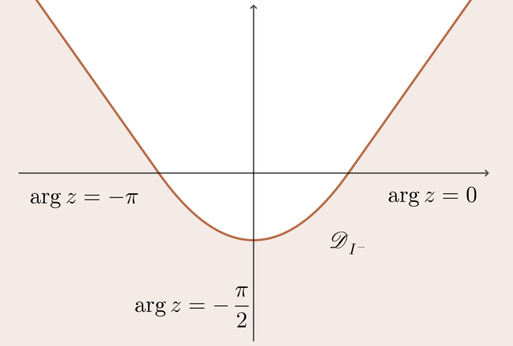
Figure 2: Left: The arcs of directions $I^{+}$ and $I^{-}$ in the Borel plane. Right: The domains $\mathscr{D}_{I^{+}}$ and $\mathscr{D}_{I^{-}}$ in the plane of the variable $z=\frac{1}{3}\lambda_{s}^{-2}$.

Theorem B.

(i) The perturbative series $\mathcal{G}_{0}=\mathcal{F}^{\hskip 0.52498pt\mathrm{s}}(\lambda_{s})$ is $1$-summable in the directions of $(-2\pi,0)$ (as well as in those of $(0,2\pi)$—cf. footnote 4) with respect to the variable $z=\frac{1}{3}\lambda_{s}^{-2}$. Each $\mathcal{G}_{n}$, $n\geqslant 1$, is $1$-summable with respect to $z$ in the directions of both

$$I^{+}\coloneqq(-\pi,0)\enspace\text{and}\enspace I^{-}\coloneqq(0,\pi).$$ (1.26)

There exist sectorial neighbourhoods of infinity $\mathscr{D}_{I^{+}}$ and $\mathscr{D}_{I^{-}}$ of opening $2\pi$, with $\mathscr{D}_{I^{\pm}}$ centred on $\arg z=\pm\frac{\pi}{2}$, such that, for each choice of sign and each $(\sigma_{1},\sigma_{2})\in\mathbb{C}^{2}$, the series of functions

$$\mathscr{S}^{I^{\pm}}\mathcal{G}(\lambda_{s},\sigma_{1},\sigma_{2})=\sigma_{1}+\sum\limits_{n\geqslant 0}\sigma_{2}^{n}\,e^{-\frac{2}{3}n\lambda_{s}^{-2}}\mathscr{S}^{I^{\pm}}\mathcal{G}_{n}(\lambda_{s})$$ (1.27)

is convergent in the domain

$$\mathscr{D}^{\pm}(\sigma_{2})\coloneqq\big{\{}z\in\mathscr{D}_{I^{\pm}}\mid\Re ez>\tfrac{1}{2}\ln|2\sigma_{2}|\big{\}}$$ (1.28)

with $z=\frac{1}{3}\lambda_{s}^{-2}$ and defines an analytic solution to the HAE (1.5).

(ii) Near the direction $\arg z=0$ (i.e. $\arg\lambda_{s}=0$), the connection between the two families of solutions is given by

$$\mathscr{S}^{I^{+}}\mathcal{G}(\lambda_{s},\sigma_{1},\sigma_{2})=\mathscr{S}^{I^{-}}\mathcal{G}(\lambda_{s},\sigma_{1},\sigma_{2}-i)$$ (1.29)

for $z=\frac{1}{3}\lambda_{s}^{-2}\in\mathscr{D}^{+}(\sigma_{2})\cap\mathscr{D}^{-}(\sigma_{2}-i).$

(iii) Near the direction $\arg z=-\pi$ (i.e. $\arg\lambda_{s}=\frac{\pi}{2}$), when $|\sigma_{2}|<1$ is small enough, there is a connection formula

$$\mathscr{S}^{I^{+}}\mathcal{G}(e^{-i\pi}\lambda_{s},\sigma_{1},\sigma_{2})=\mathscr{S}^{I^{-}}\mathcal{G}\Big{(}\lambda_{s},\sigma_{1}+\log(1+i\sigma_{2}),\frac{\sigma_{2}}{1+i\sigma_{2}}\Big{)}$$ (1.30)

in the domain $\big{\{}\,\lambda_{s}\mid z=\frac{1}{3}\lambda_{s}^{-2}\in\mathscr{D}^{-}(\frac{\sigma_{2}}{1+i\sigma_{2}})\cap(e^{-2\pi i}\mathscr{D}^{+}(\sigma_{2}))\big{\}}$.

Figure 3: The domains $\mathscr{D}_{I^{+}}\cap\mathscr{D}_{I^{-}}$ and $\mathscr{D}_{I^{-}}\cap(e^{-2\pi i}\mathscr{D}_{I^{+}})$.

Theorem B(i) gives two families of solutions, $\mathscr{S}^{I^{+}}\mathcal{G}$ and $\mathscr{S}^{I^{-}}\mathcal{G}$, parametrized by $\sigma=(\sigma_{1},\sigma_{2})$. For a given parameter $\sigma$, the corresponding solutions are a priori defined for $z=\frac{1}{3}\lambda_{s}^{-2}\in\mathscr{D}^{\pm}(\sigma_{2})$, which is a sectorial neighbourhood of infinity of opening $\pi$ only (due to the necessity of taking the intersection of $\mathscr{D}_{I^{\pm}}$ with a half-plane $\Re ez>\text{constant}$—see Figures 2 and 8). The connection formula (1.29) stems from the Stokes phenomenon across the ray $\arg\zeta=0$; it is valid for $z\in\mathscr{D}^{+}(\sigma_{2})\cap\mathscr{D}^{-}(\sigma_{2}-i)$, which is always non-empty (see the left part of Figure 3 and Figure 9), and thus implies that $\mathscr{S}^{I^{+}}\mathcal{G}$ extends analytically to $\mathscr{D}^{+}(\sigma_{2})\cup\mathscr{D}^{-}(\sigma_{2}-i)$.

The connection formula (1.30) stems from the Stokes phenomenon across the ray $\arg\zeta=\pi$, which is why it involves $\mathscr{S}^{I^{+}}\mathcal{G}(e^{-i\pi}\lambda_{s},\sigma_{1},\sigma_{2})=\mathscr{S}^{I^{+}+2\pi}\mathcal{G}(\lambda_{s},\sigma_{1},\sigma_{2})$ (because footnote 4 implies that $\mathscr{S}^{I+2\pi}\widetilde{\varphi}(z)=\mathscr{S}^{I}\widetilde{\varphi}(e^{2\pi i}z)$ and $e^{2\pi i}z$ corresponds to $e^{-i\pi}\lambda_{s}$). It is valid for $z\in\mathscr{D}^{-}(\frac{\sigma_{2}}{1+i\sigma_{2}})\cap(e^{-2\pi i}\mathscr{D}^{+}(\sigma_{2}))$; we need to require that $|\sigma_{2}|$ is sufficiently small to ensure that this intersection is non-empty (see the right part of Figure 3 and Figure 9), in which case the solution thus extends to $z\in\mathscr{D}^{-}(\frac{\sigma_{2}}{1+i\sigma_{2}})\cup(e^{-2\pi i}\mathscr{D}^{+}(\sigma_{2}))$.

Finally, we use the connection formulas to distinguish real analytic functions among the solutions $\mathscr{S}^{I^{\pm}}\mathcal{G}(\lambda_{s},\sigma_{1},\sigma_{2})$ (compare with [5]).

Theorem C.

(i) For any $a,b\in\mathbb{R}$, the particular solution

$$\mathscr{S}^{I^{+}}\mathcal{G}\big{(}\lambda_{s},a,b+\tfrac{i}{2}\big{)}=\mathscr{S}^{I^{-}}\mathcal{G}\big{(}\lambda_{s},a,b-\tfrac{i}{2}\big{)}$$ (1.31)

is analytic in $\big{\{}\,z=\frac{1}{3}\lambda_{s}^{-2}\in\mathscr{D}_{I^{+}}\cup\mathscr{D}_{I^{-}}\text{\ and\, \ }\Re ez>\frac{1}{4}\ln(1+4b^{2})\,\big{\}}$, and it is real-valued along the ray $\{\arg z=0\}$.

(ii) There exists $0<\theta_{*}<\frac{\pi}{4}$ such that, for any $a\in\mathbb{R}$ and $\theta\in(-\theta_{*},\theta_{*})$, the particular solution

$$\mathscr{S}^{I^{+}}\mathcal{G}\big{(}e^{-i\pi}\lambda_{s},a+i\tfrac{\theta}{2},i(1-e^{-i\theta})\big{)}\\ =\mathscr{S}^{I^{-}}\mathcal{G}\big{(}\lambda_{s},a-i\tfrac{\theta}{2},-i(1-e^{i\theta})\big{)}$$ (1.32)

is analytic in $\big{\{}\,z=\frac{1}{3}\lambda_{s}^{-2}\in\mathscr{D}_{I^{-}}\cup(e^{-2\pi i}\mathscr{D}_{I^{+}})\text{\ and\, \ }\Re ez>\frac{1}{2}\ln(2|1-e^{i\theta}|)\,\big{\}}$, and it is real-valued along the ray $\{\arg z=-\pi\}$.

Notice that the identities (1.31)–(1.32) are particular cases of the connection formulas (1.29)–(1.30). The condition $\arg z=0$ in Theorem C(i) is equivalent to $\arg\lambda_{s}=0$ and thus has natural physical meaning of a positive real rescaled coupling constant $\lambda_{s}=C_{zzz}(S^{zz})^{3/2}g_{s}$. However this is not the case for the condition $\arg z=-\pi$ in (ii), amounting to $\arg\lambda_{s}=\frac{\pi}{2}$, for which physical implications are yet to be found.

Corresponding to Theorems B and C, there are parallel results in the case of [9]’s large radius limit free energy for the Borel-Laplace sums of the perturbative series (1.8) and its transseries completion—see Sections 4.3 and 4.4 below, particularly Theorems B’ and C’.

1.6  Organization of the paper and outlook.

– In Section 2 we review all the essential notions and structures in resurgence theory such as Borel-Laplace summation and alien derivatives following [23], and we make it self-contained for the reader’s convenience. We seize the opportunity to add some explanations on the case of series involving non-integer powers and we give as self-contained as possible a resurgent treatment of the Airy equation.

– In Section 3 we study the all-genus free energy of the B-model topological string theory in Alim-Yau-Zhou’s double scaling limit, and its transseries completion, solution to the nonlinear ODE (1.5). We fully describe the summability properties and the resurgent structure, and compute all the alien derivatives of all the components of the two-parameter transseries, which correspond to the singularities of the analytic continuation of their Borel transforms and give us access to the Stokes phenomena associated with varying the direction in which Borel-Laplace summation is performed. As an application, real-analytic solutions can be distinguished among all possible Borel-Laplace sums.

– In Section 4, finally, we access the summability and resurgence properties of the free energy in Couso-Santamaría’s large radius limit and put [9]’s statements on a solid ground essentially by exploiting the interplay between the change of variable (4.7) and resurgence: the resurgence in $z_{1}=\frac{1}{3}\lambda_{s}^{-2}$ of the double scaling limit transseries automatically gives rise to resurgence in $z_{2}=\frac{1}{3g_{s}^{2}u^{3}}$ for the large radius transseries, which in turn can be interpreted as resurgence in $\frac{1}{g_{s}^{2}}$ for any fixed $u\in\mathbb{C}^{*}$.

Several new objects arising from the resurgence analysis, like the double scaling transseries $\widetilde{G}(z,\sigma_{1},\sigma_{2})$ of (3.18) and the large radius transseries $H^{\mathrm{u}}(g_{s},u,\sigma)$ of (1.10) (giving rise to $\mathcal{H}^{\mathrm{u}}(g_{s},u,\sigma_{1},\sigma_{2})$ in (4.6)), should have enumerative meaning from the geometric point of view, and non-perturbative implications from the topological string theory perspective—cf. Remarks 3.19 and 4.6. It would be interesting to make them manifest.

The truly challenging problem would be the complete resurgent analysis for the HAE to understand the resurgent structure of topological string free energy $\mathcal{F}(z,S^{zz})$ and its partition function. Hopefully, our methods together with the whole theory of parametric resurgence can be extended to the recursive HAE. The first attempt would be the resurgent analysis of the conjectures proposed in [17] to compare with the singularity structure in the current paper. We leave it for the future.

Acknowledgements. The 1st and 3rd author are partially supported by National Key R&D Program of China (2020YFA0713300), NSFC (No.s 11771303, 12171327, 11911530092, 12261131498, 11871045). This paper is partly a result of the ERC-SyG project, Recursive and Exact New Quantum Theory (ReNewQuantum) which received funding from the European Research Council (ERC) under the European Union’s Horizon 2020 research and innovation programm under grant agreement No 810573. This work has been partially supported by the project CARPLO of the Agence Nationale de la recherche (ANR-20-CE40-0007).

2 A brief compendium of Resurgence theory

We have briefly alluded to the definition of $\Omega$-resurgent series and alien derivations in §1, after the statement of Theorem A, and to Borel-Laplace summation in §1.1 before the statement of Theorem B. We will now expand on this, starting with more details on Borel-Laplace summation.

2.1 Borel transform, convolution and Laplace transform

For any $\nu\in\mathbb{C}$, we use the notation

$$z^{-\nu}\mathbb{C}[[z^{-1}]]\coloneqq\Big{\{}\widetilde{\varphi}(z)=\sum\limits_{n\geqslant 0}a_{n}z^{-n-\nu}\mid a_{0},a_{1},\ldots\in\mathbb{C}\Big{\}}.$$ (2.1)

In its simplest version, Resurgence Theory deals with the formal Borel transform

$$\mathscr{B}\colon\thinspace\widetilde{\varphi}(z)=\sum\limits_{n\geqslant 0}c_{n}z^{-n-1}\in z^{-1}\mathbb{C}[[z^{-1}]]\longmapsto\widehat{\varphi}(\zeta)=\sum\limits_{n\geqslant 0}c_{n}\frac{\zeta^{n}}{n!}\in\mathbb{C}[[\zeta]].$$ (2.2)

Observe that $\widehat{\varphi}(\zeta)\in\mathbb{C}\{\zeta\}$ (i.e. $\widehat{\varphi}(\zeta)$ has positive radius of convergence, and thus defines a holomorphic germ at the origin) if and only if $\widetilde{\varphi}(z)$ is a $1$-Gevrey formal power series, i.e. there exist $A,B>0$ such that $|c_{n}|\leqslant AB^{n}n!$ for all $n\geqslant 0.$

The convolution product of two holomorphic germs $\widehat{\varphi},\widehat{\psi}\in\mathbb{C}\{\zeta\}$, defined as

$$\widehat{\varphi}\ast\widehat{\psi}(\zeta)\coloneqq\int_{0}^{\zeta}\widehat{\varphi}(\xi)\widehat{\psi}(\zeta-\xi)d\xi,$$ (2.3)

is easily seen to be a holomorphic germ itself (this makes $\mathbb{C}\{\zeta\}$ a commutative associative algebra without unit), and $(\mathscr{B}^{-1}\widehat{\varphi})(\mathscr{B}^{-1}\widehat{\psi})=\mathscr{B}^{-1}(\widehat{\varphi}*\widehat{\psi})$.

If $\mathop{\Re e}\nolimits\nu>0$, then the formal Borel transform extends to

$$\mathscr{B}\colon\thinspace\widetilde{\varphi}(z)=\sum\limits c_{\mu}z^{-\mu}\in z^{-\nu}\mathbb{C}[[z^{-1}]]\longmapsto\widehat{\varphi}=\sum\limits c_{\mu}\tfrac{\zeta^{\mu-1}}{\Gamma(\mu)}\in\zeta^{\nu-1}\mathbb{C}[[\zeta]]$$ (2.4)

and, if also $\mathop{\Re e}\nolimits\nu^{\prime}>0$, formula (2.3) naturally extends to

$$\widehat{\varphi}\in\zeta^{\nu-1}\mathbb{C}\{\zeta\},\;\widehat{\psi}\in\zeta^{\nu^{\prime}-1}\mathbb{C}\{\zeta\} \enspace\Longrightarrow\enspace\widehat{\varphi}*\widehat{\psi}\in\zeta^{\nu+\nu^{\prime}-1}\mathbb{C}\{\zeta\}$$ (2.5)

$$\quad\enspace\Longrightarrow\enspace(\mathscr{B}^{-1}\widehat{\varphi})(\mathscr{B}^{-1}\widehat{\psi})=\mathscr{B}^{-1}(\widehat{\varphi}*\widehat{\psi}).$$ (2.6)

The motivation is that the Laplace transform (1.23) satisfies

$$\mathscr{L}^{\theta}\Big{(}\frac{\zeta^{\mu-1}}{\Gamma(\mu)}\Big{)}(z)=z^{-\mu}\quad\text{for any~$z$ in the half-plane $\{\mathop{\Re e}\nolimits(e^{i\theta}z)>0\}$}$$

provided $\mathop{\Re e}\nolimits\mu>0$, and

$$\mathscr{L}^{\theta}(\widehat{\varphi}*\widehat{\psi})=(\mathscr{L}^{\theta}\widehat{\varphi})(\mathscr{L}^{\theta}\widehat{\psi})$$ (2.7)

if $\widehat{\varphi}$ and $\widehat{\psi}$ can be subjected to Laplace transform, which requires them to be integrable at $0$.

2.2 Borel-Laplace summation of formal power series

For $\mathscr{L}^{\theta}\widehat{\varphi}$ to be defined, even if $\widehat{\varphi}(\zeta)$ is a holomorphic function regular at $0$ and along the ray $e^{i\theta}\mathbb{R}_{\geqslant 0}$, we must impose an exponential bound of the form

$$|\widehat{\varphi}(re^{i\theta})|\leqslant\beta(\theta)e^{\alpha(\theta)r}\quad\text{for all $r>0$,}$$ (2.8)

for some $\alpha(\theta),\beta(\theta)\in\mathbb{R}$. In fact, it is convenient to work with

Definition 2.1.

– Let $I\subset\mathbb{R}$ denote an open interval and $\alpha:I\rightarrow\mathbb{R}$ a locally bounded function. We denote by $\displaystyle\mathscr{N}(I,\alpha)$ the set of all $\widehat{\varphi}(\zeta)\in\mathbb{C}\{\zeta\}$ that have an analytic continuation to the open sector $\{\arg\zeta\in I\}$ and for which, for every $\epsilon>0$, there exists a locally bounded function $\beta:I\rightarrow\mathbb{R}_{\geqslant 0}$ such that

$$|\widehat{\varphi}(re^{i\theta})|\leqslant\beta(\theta)e^{(\alpha(\theta)+\epsilon)r}\quad\text{for all $r>0$ and $\theta\in I$.}$$ (2.8’)

– We set $\displaystyle\widetilde{\mathscr{N}}(I,\alpha)\coloneqq\mathscr{B}^{-1}\big{(}\mathscr{N}(I,\alpha)\big{)}\subset z^{-1}\mathbb{C}[[z^{-1}]]$ and $\displaystyle\widetilde{\mathscr{N}}(I)\coloneqq\bigcup_{\alpha}\displaystyle\widetilde{\mathscr{N}}(I,\alpha)$.

Since locally bounded functions are precisely those functions that are bounded on any compact subinterval, imposing bounds of the form (2.8) or (2.8’) along $I$ with some locally bounded functions $\alpha$ and $\beta$ is equivalent to imposing uniform bounds of the form (1.22) for every compact subinterval $J\subset\joinrel\subset I$.

Given $\widehat{\varphi}\in\mathscr{N}(I,\alpha)$, (1.23) yields a Laplace transform $\mathscr{L}^{\theta}\widehat{\varphi}$ holomorphic in

$$\Pi^{\theta}_{\alpha(\theta)}\coloneqq\{z\in\mathbb{C}\mid\mathop{\Re e}\nolimits(z\,e^{i\theta})>\alpha(\theta)\}$$ (2.9)

for each $\theta\in I$ (this is the half-plane bisected by $e^{-i\theta}\mathbb{R}_{\geqslant 0}$ that has $\alpha(\theta)e^{-i\theta}$ on its boundary—cf. Figure 1). One can check that, for any $\theta,\theta^{\prime}\in I$ such that $|\theta^{\prime}-\theta|<\pi$, the half-planes $\Pi^{\theta}_{\alpha(\theta)}$ and $\Pi^{\theta^{\prime}}_{\alpha(\theta^{\prime})}$ have a non-empty intersection, in which $\mathscr{L}^{\theta}\widehat{\varphi}$ and $\mathscr{L}^{\theta^{\prime}}\widehat{\varphi}$ coincide (by the Cauchy theorem—cf. [23, p. 142]). We can thus glue together the various functions obtained by varying $\theta$ continuously, but with a grain of salt if $|I|>\pi$, because $\pi<|\theta^{\prime}-\theta|<2\pi\,\Longrightarrow\,\Pi^{\theta}_{\alpha(\theta)}\cap\Pi^{\theta^{\prime}}_{\alpha(\theta^{\prime})}\neq\emptyset$ but nothing guarantees that $\mathscr{L}^{\theta}\widehat{\varphi}$ and $\mathscr{L}^{\theta^{\prime}}\widehat{\varphi}$ agree on that subset of $\mathbb{C}$. The remedy is to consider a universal cover $\widetilde{\mathscr{D}}(I,\alpha)$ of

$$\underline{\mathscr{D}}(I,\alpha)\coloneqq\bigcup_{\theta\in I}\Pi^{\theta}_{\alpha(\theta)}\subset\mathbb{C}.$$ (2.10)

Note that the canonical projection $\widetilde{\mathscr{D}}(I,\alpha)\to\underline{\mathscr{D}}(I,\alpha)$ is a homeomorphism if $|I|<\pi$, but it may be many-to-one if $|I|>\pi$. We thus pick a lift $\widetilde{\Pi}\,\!^{\theta}_{\alpha(\theta)}\subset\widetilde{\mathscr{D}}(I,\alpha)$ of $\Pi^{\theta}_{\alpha(\theta)}$ that depends continuously on $\theta$, and define

$$\mathscr{D}(I,\alpha)\coloneqq\bigcup_{\theta\in I}\widetilde{\Pi}\,\!^{\theta}_{\alpha(\theta)}\subset\widetilde{\mathscr{D}}(I,\alpha).$$ (2.11)

Definition 2.2.

– The Laplace transform in the directions of $I$ is the operator $\widehat{\varphi}\in\mathscr{N}(I,\alpha)\mapsto\mathscr{L}^{I}\widehat{\varphi}$, where $\mathscr{L}^{I}\widehat{\varphi}$ is the holomorphic function defined by

$$z\in\mathscr{D}(I,\alpha)\mapsto\mathscr{L}^{I}\widehat{\varphi}(z)\coloneqq\mathscr{L}^{\theta}\widehat{\varphi}(z)\enspace\text{for any $\theta\in I$ such that $z\in\widetilde{\Pi}\,\!^{\theta}_{\alpha(\theta)}$}$$ (2.12)

(any two values of $\theta$ such that $z\in\widetilde{\Pi}\,\!^{\theta}_{\alpha(\theta)}$ result in the same value of $\mathscr{L}^{\theta}\widehat{\varphi}(z)$).

– The Borel-Laplace summation operator in the directions of $I$ is

$$\mathscr{S}^{I}\coloneqq\mathscr{L}^{I}\circ\mathscr{B}\colon\thinspace\widetilde{\mathscr{N}}(I,\alpha)\to\mathscr{O}\big{(}\mathscr{D}(I,\alpha)\big{)}.$$ (2.13)

Remark 2.3.

If $\alpha\geqslant 0$, then $0$ is in the complement of $\underline{\mathscr{D}}(I,\alpha)$ and we can view $\widetilde{\mathscr{D}}(I,\alpha)$ as a subset of the universal cover $\widetilde{\mathbb{C}}$ of $\mathbb{C}\setminus\{0\}$, i.e. of the Riemann surface of the logarithm on which there is a well-defined argument function $\arg\colon\thinspace\widetilde{\mathbb{C}}\to\mathbb{R}$. Our choice for the lifts $\widetilde{\Pi}\,\!^{\theta}_{\alpha(\theta)}$ is then so that

$$I=(\theta_{1},\theta_{2})\enspace\Longrightarrow\enspace\mathscr{D}(I,\alpha)\coloneqq\{\,z\in\widetilde{\mathbb{C}}\mid\arg z\in(-\theta_{2}-\tfrac{\pi}{2},-\theta_{1}+\tfrac{\pi}{2}),\\ \exists\,\theta\in I\;\text{such that}\;\mathop{\Re e}\nolimits(ze^{i\theta})>\alpha(\theta)\,\}$$ (2.14)

in harmony with the convention indicated in footnote 4.

At this point, we have the commutative diagram

(2.15)

It is easy to check that $\mathscr{N}(I,\alpha)$ is stable under convolution, thus $\widetilde{\mathscr{N}}(I,\alpha)$ is stable under Cauchy product and (2.7) yields

$$\widehat{\varphi},\widehat{\psi} \in\mathscr{N}(I,\alpha) \quad\Longrightarrow\quad \mathscr{L}^{I}(\widehat{\varphi}*\widehat{\psi}) =(\mathscr{L}^{I}\widehat{\varphi})(\mathscr{L}^{I}\widehat{\psi})$$ (2.16)

$$\widetilde{\varphi},\widetilde{\psi} \in\widetilde{\mathscr{N}}(I,\alpha) \quad\Longrightarrow\quad \mathscr{S}^{I}(\widetilde{\varphi}\,\widetilde{\psi}) =(\mathscr{S}^{I}\widetilde{\varphi})(\mathscr{S}^{I}\widetilde{\psi}).$$ (2.17)

It follows that $\mathbb{C}\oplus\widetilde{\mathscr{N}}(I,\alpha)$ is a subalgebra of $\mathbb{C}[[z^{-1}]]$ and we can extend $\mathscr{S}^{I}$ into an algebra homomorphism

$$\mathscr{S}^{I}\colon\thinspace\mathbb{C}\oplus\widetilde{\mathscr{N}}(I,\alpha)\to\mathscr{O}\big{(}\mathscr{D}(I,\alpha)\big{)}$$ (2.18)

by setting $\mathscr{S}^{I}(1)\coloneqq 1$ (this is equivalent to (1.25)). Correspondingly, setting $\mathscr{B}1=\delta$ and $\mathscr{L}^{I}\delta=1$, we can embed $\mathscr{N}(I,\alpha)$ into the convolution algebra $\mathbb{C}\delta\oplus\mathscr{N}(I,\alpha)$ (which amounts to adjunction of unit) and upgrade (2.15) to a commutative diagram of unital algebras

(2.15’)

Remark 2.4.

Convergent series are $1$-summable in all directions: given an arbitrary interval $I$, if a formal series $\widetilde{\varphi}(z)$ is convergent for $|z^{-1}|<\rho$, then $\widetilde{\varphi}\in\mathbb{C}\oplus\widetilde{\mathscr{N}}(I,\alpha)$ for any $\alpha\geqslant\rho^{-1}$ and $\mathscr{S}^{I}\widetilde{\varphi}(z)$ coincides with the usual sum of $\widetilde{\varphi}(z)$ for $z\in\mathscr{D}(I,\alpha)$ (because the Borel transform is then an entire function of bounded exponential type in all directions).

2.3 Extension to non-integer powers

Since $\mathbb{C}\oplus\widetilde{\mathscr{N}}(I,\alpha)\subset\mathbb{C}[[z^{-1}]]$, so far we’ve been dealing with formal series involving only non-positive integer powers, but sometimes one needs formal power series involving positive integer powers or even complex non-integer powers, typically finite sums

$$\widetilde{\varphi}=\widetilde{\varphi}_{1}+\cdots+\widetilde{\varphi}_{N}\quad\text{with}\enspace\widetilde{\varphi}_{j}\in z^{-\mu_{j}}\mathbb{C}[[z^{-1}]],\quad\mu_{j}\in\mathbb{C}.$$ (2.19)

We use the notation $\sum\limits_{\mu\in\mathbb{C}}z^{-\mu}\mathbb{C}[[z^{-1}]]$ for the vector space of all such expressions $\widetilde{\varphi}$ (meant as a sum of vector spaces that is not a direct sum, due to the natural inclusions $z^{-\mu-\Delta}\mathbb{C}[[z^{-1}]]\subset z^{-\mu}\mathbb{C}[[z^{-1}]]$ for any $\mu\in\mathbb{C}$ and $\Delta\in\mathbb{Z}_{\geqslant 0}$—see (A.1)).

Definition 2.5.

Given an open interval $I\subset\mathbb{R}$ and a locally bounded function $\alpha\colon\thinspace I\to\mathbb{R}$, we define ${\widetilde{\mathscr{N}}_{\text{ext}}}(I,\alpha)$ as the set of all $\widetilde{\varphi}$ of the form (2.19) where

$$z^{\mu_{j}}\widetilde{\varphi}_{j}\in\widetilde{\mathscr{N}}(I,\alpha)\quad\text{for $j=1,\ldots,N$,}$$ (2.20)

i.e. ${\widetilde{\mathscr{N}}_{\text{ext}}}(I,\alpha)\coloneqq\sum\limits_{\mu\in\mathbb{C}}z^{-\mu}\widetilde{\mathscr{N}}(I,\alpha)$. The set of all formal series $1$-summable in the directions of $I$ is defined to be $\displaystyle{\widetilde{\mathscr{N}}_{\text{ext}}}(I)\coloneqq\bigcup_{\alpha}{\widetilde{\mathscr{N}}_{\text{ext}}}(I,\alpha)$.

Suppose $\alpha\geqslant 0$. We define the Borel-Laplace sum of any $\widetilde{\varphi}\in{\widetilde{\mathscr{N}}_{\text{ext}}}(I,\alpha)$ in the directions of $I$ as the holomorphic function

$$\mathscr{S}^{I}\widetilde{\varphi}\coloneqq z^{-\mu_{1}}\mathscr{S}^{I}(z^{\mu_{1}}\widetilde{\varphi}_{1})+\cdots+z^{-\mu_{N}}\mathscr{S}^{I}(z^{\mu_{N}}\widetilde{\varphi}_{N})\in\mathscr{O}\big{(}\mathscr{D}(I,\alpha)\big{)}$$ (2.21)

for any decomposition of $\widetilde{\varphi}$ satisfying (2.19)–(2.20)—the right-hand side of (2.21) does not depend of the choice of that decomposition because

$$\widetilde{\psi}\in\widetilde{\mathscr{N}}(I,\alpha)\quad\Longrightarrow\quad\mathscr{S}^{I}(z^{-\Delta}\widetilde{\psi})=z^{-\Delta}\mathscr{S}^{I}\widetilde{\psi}$$ (2.22)

for any $\Delta\in\mathbb{Z}_{>0}$. See Appendix A for more details.

One can check that ${\widetilde{\mathscr{N}}_{\text{ext}}}(I,\alpha)\subset\sum\limits_{\nu\in\mathbb{C}}z^{-\nu}\mathbb{C}[[z^{-1}]]$ inherits from the Cauchy product in $\mathbb{C}[[z^{-1}]]$ a product law that makes it a commutative associative algebra, and the Borel-Laplace summation operator

$$\mathscr{S}^{I}\colon\thinspace{\widetilde{\mathscr{N}}_{\text{ext}}}(I,\alpha)\to\mathscr{O}\big{(}\mathscr{D}(I,\alpha)\big{)}$$ (2.23)

is an algebra homomorphism. Moreover, ${\widetilde{\mathscr{N}}_{\text{ext}}}(I,\alpha)$ is stable under $\frac{d\,}{dz}$ and

$$\mathscr{S}^{I}\Big{(}\frac{d\widetilde{\varphi}}{dz}\Big{)}=\frac{d\,}{dz}\big{(}\mathscr{S}^{I}\widetilde{\varphi}\big{)}$$ (2.24)

ultimately because

$$\widetilde{\psi}\in\mathbb{C}[[z^{-1}]]\enspace\Longrightarrow\enspace\mathscr{B}\Big{(}\frac{d\widetilde{\psi}}{dz}\Big{)}=-\zeta\mathscr{B}\widetilde{\psi}(\zeta).$$ (2.25)

Finally, one can check that $z\widetilde{\mathscr{N}}(I)=\mathbb{C}\oplus\widetilde{\mathscr{N}}(I)$ and, in restriction to

$${\widetilde{\mathscr{N}}_{\text{ext}}}^{-}(I,\alpha)\coloneqq\sum_{\mathop{\Re e}\nolimits\mu>-1}z^{-\mu}\widetilde{\mathscr{N}}(I)=\sum_{\mathop{\Re e}\nolimits\nu>0}z^{-\nu}\big{(}\mathbb{C}\oplus\widetilde{\mathscr{N}}(I)\big{)},$$ (2.26)

our extended Borel-Laplace summation operator $\mathscr{S}^{I}$ satisfies

$$\mathscr{S}^{I}=\mathscr{L}^{I}\circ\mathscr{B}$$ (2.27)

with $\mathscr{B}$ as in (2.4), and with a convention for $\mathscr{L}^{I}$ naturally deduced from (1.23) and (2.12) (just because (2.22) holds for any $\Delta\in\mathbb{C}$ with $\mathop{\Re e}\nolimits\Delta>0$). However, one cannot define the Borel transform of an element of ${\widetilde{\mathscr{N}}_{\text{ext}}}(I)$ as a proper function when it does not belong to ${\widetilde{\mathscr{N}}_{\text{ext}}}^{-}(I)$; the Borel transform of $1$ was defined above as $\delta$, which is a symbol that can be identified with the Dirac mass at $0$, and in general one must resort to the formalism of majors [12, 26].

2.4 Asymptotic expansion property, compatibility with composition

Let $I$ denote an open interval of $\mathbb{R}$. Any $1$-summable formal series $\widetilde{\varphi}\in{\widetilde{\mathscr{N}}_{\text{ext}}}(I)$ appears as the asymptotic expansion at infinity of its Borel-Laplace sum $\mathscr{S}^{I}\widetilde{\varphi}$, with $1$-Gevrey qualification:

$$\mathscr{S}^{I}\widetilde{\varphi}(z)\sim_{1}\widetilde{\varphi}(z)\enspace\text{in}\;\mathscr{D}(I,\alpha),\quad\text{for some $\alpha\colon\thinspace I\to\mathbb{R}_{>0}$}.$$

When $\widetilde{\varphi}(z)=\sum\limits_{n\geqslant 0}a_{n}z^{-n}\in\mathbb{C}\oplus\widetilde{\mathscr{N}}(I)$, this means that there exists a locally bounded function $\alpha\colon\thinspace I\to\mathbb{R}_{>0}$, such that, for every $J\subset\joinrel\subset I$, there are constants $L,M>0$ such that

$$|\mathscr{S}^{I}\widetilde{\varphi}(z)-a_{0}-a_{1}z^{-1}-\cdots-a_{N-1}z^{-(N-1)}|\leqslant LM^{N}N!|z|^{-N}$$

for every $z\in\mathscr{D}(J,\alpha|_{J})$ and $N\in\mathbb{Z}_{\geqslant 0}$. In the general case, the formulation of the asymptotic expansion property must be adjusted to take into account the exponents $-\mu_{j}-n-1$ that stem from (2.21).

Another property of the space of $1$-summable formal series that we will use is its stability under nonlinear operations, as expressed in

Theorem 2.6 ([23, Theorem 5.55]).

Suppose $H(t)=\sum\limits_{n=0}^{\infty}H_{n}t^{n}\in\mathbb{C}\{t\}$, $\widetilde{\varphi}_{*}\in\mathscr{N}(I)$, and $\widetilde{\varphi},\widetilde{\psi}\in\mathbb{C}\oplus\mathscr{N}(I)$. Then the formal series

$$H\circ\widetilde{\varphi}_{*}\coloneqq\sum\limits_{n=0}^{\infty}H_{n}\widetilde{\varphi}_{*}^{n}\quad\text{and}\quad\widetilde{\psi}\circ(id+\widetilde{\varphi})\coloneqq\sum\limits_{n\geqslant 0}\frac{1}{n!}\widetilde{\varphi}^{n}\partial^{n}\widetilde{\psi}$$ (2.28)

are 1-summable in the directions of I, with

$$\mathscr{S}^{I}(H\circ\widetilde{\varphi}_{*})=H\circ(\mathscr{S}^{I}\widetilde{\varphi}_{*})\quad\text{and}\quad\mathscr{S}^{I}(\widetilde{\psi}\circ(id+\widetilde{\varphi}))=(\mathscr{S}^{I}\widetilde{\psi})\circ(id+\mathscr{S}^{I}\widetilde{\varphi}).$$ (2.29)

2.5 Example: Asymptotics of the solutions to the Airy equation

Since, according to [3], Alim-Yau-Zhou’s double scaling limit partition function $\mathcal{Z}_{\mathrm{top},\mathrm{s}}=\exp\mathcal{F}^{\hskip 0.52498pt\mathrm{s}}$ solves the Airy equation (1.6) (up to an elementary factor), we recall here the first steps of the resurgent treatment of the Airy equation following [23, Sec. 6.14]. We will use the same formal series $\widetilde{\psi}(z)$ and $\widetilde{\varphi}(z)\coloneqq\widetilde{\psi}(-z)$ as in [23], which will play a key role in Sections 3 and 4.

2.5.1  As a preliminary step, the change of variable and unknown

$$z=\tfrac{2}{3}w^{\frac{3}{2}},\qquad y(w)=w\,e^{z}A(z)$$ (2.30)

is seen to bring the Airy equation $\frac{d^{2}y}{dw^{2}}=wy$ to the form

$$A^{\prime\prime}+2A^{\prime}+\tfrac{5}{3}z^{-1}(A^{\prime}+A)=0.$$ (2.31)

For arbitrary $\nu\in\mathbb{C}$, we look for a solution of the form $z^{-\nu}\big{(}1+O(z^{-1})\big{)}$ to the linear ODE (2.31) in the space of formal series $z^{-\nu}\mathbb{C}[[z^{-1}]]$. Since the dominant part of the left-hand side is $2A^{\prime}+\frac{5}{3}z^{-1}A$, we must impose $-2\nu+\frac{5}{3}=0$: the only possibility is $\nu=\frac{5}{6}$, and one easily finds that there is a unique formal solution $\widetilde{A}(z)$, whose coefficients can be determined inductively.

Let us consider the Borel transform of $\widetilde{A}(z)=z^{-\frac{5}{6}}\big{(}1+O(z^{-1})\big{)}\in z^{-\frac{5}{6}}\mathbb{C}[[z^{-1}]]$:

$$\widehat{A}(\zeta)\coloneqq\mathscr{B}\widetilde{A}=\tfrac{\zeta^{-\frac{1}{6}}}{\Gamma(\frac{5}{6})}\big{(}1+O(\zeta)\big{)}\in\zeta^{-\frac{1}{6}}\mathbb{C}[[\zeta]].$$ (2.32)

Since $\mathscr{B}(\widetilde{A}^{\prime})=-\zeta\widehat{A}(\zeta)$ and $\mathscr{B}z^{-1}=1$, the formal series $\widehat{A}(\zeta)$ must be the unique solution of the form (2.32) to the Borel transformed equation

$$\zeta^{2}\widehat{A}(\zeta)-2\zeta\widehat{A}(\zeta)+\tfrac{5}{3}1*\big{(}\!-\zeta\widehat{A}(\zeta)+\widehat{A}(\zeta)\big{)}=0,$$ (2.33)

which is equivalent (upon differentiation with respect to $\zeta$) to

$$\frac{d\,}{d\zeta}\big{(}(\zeta^{2}-2\zeta)\widehat{A}\big{)}+\tfrac{5}{3}(1-\zeta)\widehat{A}=0,$$ (2.34)

thus $\widehat{A}(\zeta)$ must be proportional to $(\zeta-\zeta^{2}/2)^{-\frac{1}{6}}$. Therefore

$$\widehat{A}(\zeta)=\tfrac{\zeta^{-\frac{1}{6}}}{\Gamma(\frac{5}{6})}(1-\tfrac{\zeta}{2})^{-\frac{1}{6}}=\sum_{n\geqslant 0}\frac{\Gamma(n+\frac{1}{6})}{2^{n}n!\Gamma(\frac{1}{6})\Gamma(\frac{5}{6})}\zeta^{n-\frac{1}{6}}.$$ (2.35)

We see that $\widehat{A}(\zeta)\in\zeta^{-\frac{1}{6}}\mathbb{C}\{\zeta\}$ defines a holomorphic germ on the Riemann surface of the logarithm for $|\zeta|$ small enough, that has an analytic continuation to $\{\arg\zeta\notin 2\pi\mathbb{Z}\}\subset\widetilde{\mathbb{C}}$. In fact,

$$\widehat{A}\in\zeta^{-\frac{1}{6}}\mathscr{N}(I_{0},0)\quad\text{with}\enspace I_{0}\coloneqq(-2\pi,0)$$ (2.36)

because $\theta\in I_{0}\mapsto\beta(\theta)\coloneqq\sup\limits_{\arg\zeta=\theta}|(1-\frac{\zeta}{2})^{-\frac{1}{6}}|$ defines a locally bounded function, and the formal solution $\widetilde{A}(z)$ to (2.31) is divergent.

2.5.2  Since $\frac{\zeta^{-\frac{5}{6}}}{\Gamma(\frac{1}{6})}*\frac{\zeta^{n-\frac{1}{6}}}{\Gamma(n+\frac{5}{6})}=\mathscr{B}(z^{-\frac{1}{6}}z^{-n-\frac{5}{6}})=\zeta^{n}/n!$ by the last part of (2.6), we obtain integer powers by considering

$$\widehat{B}(\zeta)\coloneqq\frac{\zeta^{-\frac{5}{6}}}{\Gamma(\frac{1}{6})}*\widehat{A}=\sum_{n\geqslant 0}c_{n}\frac{\zeta^{n}}{n!},\quad\text{with}\enspace c_{n}\coloneqq\frac{\Gamma(n+\frac{1}{6})\Gamma(n+\frac{5}{6})}{2^{n}n!\Gamma(\frac{1}{6})\Gamma(\frac{5}{6})}.$$ (2.37)

The first part of (2.6) shows that $\widehat{B}(\zeta)\in\mathbb{C}\{\zeta\}$ and, for $\arg\zeta=\theta\in I_{0}$, the inequality $|\widehat{A}(\zeta)|\leqslant\beta(\theta)|\zeta|^{-\frac{1}{6}}/\Gamma(\frac{5}{6})$ entails $|\widehat{B}(\zeta)|\leqslant\int_{0}^{1}\frac{|t\zeta|^{-\frac{5}{6}}}{\Gamma(\frac{5}{6})}|\widehat{A}\big{(}(1-t)\zeta\big{)}\zeta|dt\leqslant\beta(\theta)$, whence

$$\widehat{B}\in\mathscr{N}(I_{0},0),\qquad\widetilde{B}(z)\coloneqq\mathscr{B}^{-1}\widehat{B}=z^{-\frac{1}{6}}\widetilde{A}(z)=\sum_{n\geqslant 0}c_{n}z^{-n-1}\in\widetilde{\mathscr{N}}(I_{0},0)$$ (2.38)

(the function $\widehat{B}(\zeta)=\frac{\zeta^{-\frac{5}{6}}}{\Gamma(\frac{1}{6})}*\frac{1}{\Gamma(\frac{5}{6})}(\zeta-\frac{\zeta^{2}}{2})^{-\frac{1}{6}}$ is denoted by $\widehat{\chi}(-\zeta)$ in [23, Sec. 6.14]).

Finally, we set

$$\widetilde{\psi}(z)\coloneqq z\widetilde{B}(z)=z^{\frac{5}{6}}\widetilde{A}(z)=\sum_{n\geqslant 0}c_{n}z^{-n}.$$ (2.39)

The formal series $\widetilde{\psi}(z)$ is divergent, and $\widetilde{\psi}\in\mathbb{C}\oplus\widetilde{\mathscr{N}}(I_{0},0)$ because

$$\widehat{\psi}\coloneqq\mathscr{B}\widetilde{\psi}=\delta+\frac{d\widehat{B}}{d\zeta}\in\mathbb{C}\delta\oplus\mathscr{N}(I_{0},0)$$ (2.40)

(the Cauchy inequalities yield a uniform bound for $|\frac{d\widehat{B}}{d\zeta}(\zeta)|$ for $\arg\zeta$ restricted to any compact subinterval $J\subset\joinrel\subset I_{0}$).

2.5.3  From $\widetilde{\psi}(z)=z^{\frac{5}{6}}\widetilde{A}(z)$ and (2.31), we deduce that $\widetilde{\psi}(z)$ is the unique solution in $\mathbb{C}[[z^{-1}]]$ with constant term $1$ to the linear ODE

$$\psi^{\prime\prime}+2\psi^{\prime}+\frac{5}{36}z^{-2}\psi=0.$$ (2.41)

By Borel-Laplace summation, we get a function

$$\mathscr{S}^{I_{0}}\widetilde{\psi}\enspace\text{holomorphic in}\enspace\mathscr{D}(I_{0},0)=\big{\{}z\in\widetilde{\mathbb{C}}\mid-\tfrac{\pi}{2}<\arg z<\tfrac{5\pi}{2}\big{\}}$$ (2.42)

that is $1$-Gevrey asymptotic to $\widetilde{\psi}(z)$ and solves (2.41) (thanks to (2.17) and (2.24)).

Undoing the change (2.30), we get a particular solution $y(w)$ to the Airy equation (1.6):

$$y(w)\coloneqq\tfrac{1}{2i\sqrt{\pi}}\,w^{-\frac{1}{4}}\,e^{\frac{2}{3}w^{3/2}}\mathscr{S}^{I_{0}}\widetilde{\psi}\big{(}\tfrac{2}{3}w^{\frac{3}{2}}\big{)}\sim_{\frac{2}{3}}\tfrac{1}{2i\sqrt{\pi}}\,w^{-\frac{1}{4}}\,e^{\frac{2}{3}w^{3/2}}(1+\tfrac{3}{2}c_{1}w^{-\frac{3}{2}}+\cdots),$$ (2.43)

where the $\frac{2}{3}$-Gevrey asymptotic expansion property (see [23, § 6.14.2]) holds in the sector $-\frac{\pi}{3}<\arg w<\frac{5\pi}{3}$ (in particular this $y(w)$ is exponentially small at infinity for $\frac{\pi}{3}<\arg w<\pi$).

2.5.4  Similarly, still with the change of variable $z=\tfrac{2}{3}w^{\frac{3}{2}}$, but with the change of unknown

$$y(w)=w\,e^{-z}A_{+}(z),$$ (2.44)

we get the linear ODE

$$A_{+}^{\prime\prime}-2A_{+}^{\prime}+\tfrac{5}{3}z^{-1}(A_{+}^{\prime}-A_{+})=0,$$ (2.45)

leading to the divergent formal solution

$$\widetilde{A}_{+}(z)\coloneqq\mathscr{B}^{-1}\Big{[}\tfrac{\zeta^{-\frac{1}{6}}}{\Gamma(\frac{5}{6})}(1+\tfrac{\zeta}{2})^{-\frac{1}{6}}\Big{]}\in z^{\frac{1}{6}}\widetilde{\mathscr{N}}(I_{\pi},0)\subset z^{-\frac{5}{6}}\mathbb{C}[[z^{-1}]]\enspace\text{with}\;I_{\pi}\coloneqq(-\pi,\pi).$$ (2.46)

We get

$$\widehat{B}_{+}(\zeta) \coloneqq\frac{\zeta^{-\frac{5}{6}}}{\Gamma(\frac{1}{6})}*\frac{1}{\Gamma(\frac{5}{6})}\Big{(}\zeta+\frac{\zeta^{2}}{2}\Big{)}^{-\frac{1}{6}}=\widehat{B}(-\zeta)\in\mathscr{N}(I_{\pi},0)$$ (2.47)

$$\widetilde{B}_{+}(\zeta) =z^{-1/6}\widetilde{A}_{+}(z)=-\widetilde{B}(-z)\in\widetilde{\mathscr{N}}(I_{\pi},0).$$ (2.48)

We thus arrive at

$$\widetilde{\varphi}(z)\coloneqq z\widetilde{B}_{+}(z)=\widetilde{\psi}(-z)=\sum_{n\geqslant 0}(-1)^{n}c_{n}z^{-n}\in\mathbb{C}\oplus\widetilde{\mathscr{N}}(I_{\pi},0)$$ (2.49)

divergent formal solution to

$$\varphi^{\prime\prime}-2\varphi^{\prime}+\frac{5}{36}z^{-2}\varphi=0$$ (2.50)

and giving rise to the analytic solution $\mathscr{S}^{I_{\pi}}\widetilde{\varphi}$, holomorphic in $\mathscr{D}(I_{\pi},0)=\{z\in\widetilde{\mathbb{C}}\mid-\frac{3\pi}{2}<\arg z<\frac{3\pi}{2}\}$. The corresponding solution to the Airy equation (1.6) is

$$y_{+}(w)\coloneqq\tfrac{1}{2\sqrt{\pi}}\,w^{-\frac{1}{4}}\,e^{-\frac{2}{3}w^{3/2}}\mathscr{S}^{I_{\pi}}\widetilde{\varphi}\big{(}\tfrac{2}{3}w^{\frac{3}{2}}\big{)}\sim_{\frac{2}{3}}\tfrac{1}{2\sqrt{\pi}}\,w^{-\frac{1}{4}}\,e^{-\frac{2}{3}w^{3/2}}(1-\tfrac{3}{2}c_{1}w^{-\frac{3}{2}}+\cdots),$$ (2.51)

which is nothing but the Airy function $\operatorname{Ai}(w)$. It has $\frac{2}{3}$-Gevrey asymptotic behaviour similar to (2.43), but in the sector $-\pi<\arg w<\pi$ (in particular, it is exponentially small at infinity for $-\frac{\pi}{3}<\arg w<\frac{\pi}{3}$).

Remark 2.7.

There is a relation with the hypergeometric function:

$${}_{2}\text{\bf{F}}_{1}\big{(}\tfrac{5}{6},\tfrac{1}{6};1;-\xi\big{)}=\widehat{B}_{+}(2\xi)=\tfrac{\xi^{-\frac{5}{6}}}{\Gamma(\frac{1}{6})}*\big{[}\tfrac{\xi^{-\frac{1}{6}}}{\Gamma(\frac{5}{6})}(1+\xi)^{-\frac{1}{6}}\big{]}.$$ (2.52)

More generally, for any $a,b,c\in\mathbb{C}$,

$$\mathop{\Re e}\nolimits c>\mathop{\Re e}\nolimits a>0\quad\Longrightarrow\quad\xi^{1-c}\cdot{}_{2}\text{\bf{F}}_{1}(a,b;c;-\xi)=\tfrac{\xi^{c-a-1}}{\Gamma(c-a)}*\big{[}\tfrac{\xi^{a-1}}{\Gamma(a)}(1+\xi)^{-b}\big{]}.$$ (2.53)

2.6 Alien calculus for simple $\Omega$-resurgent series

We now give ourselves a lattice $\Omega$ of $\mathbb{C}$, of rank $1$ for the sake of simplicity. Thus $\Omega=\omega_{1}\cdot\mathbb{Z}$, where $\omega_{1}\in\mathbb{C}^{\ast}$ is one of the two generators of $\Omega$.

We will give details about the alien operators labelled by the points of $\Omega$ in the case of simple resurgent series, as well as some indications for the more general framework (for which the reader should consult [12], [26], [27]).

For $R>0$ and $\zeta_{0}\in\mathbb{C}$ we use the notations $D(\zeta_{0},R)\coloneqq\{\,\zeta\in\mathbb{C}\mid|\zeta-\zeta_{0}|<R\,\}$,

$$D^{*}(\zeta_{0},R)\coloneqq D(\zeta_{0},R)\setminus\{\zeta_{0}\},\quad\mathbb{D}_{R}\coloneqq D(0,R),\quad\mathbb{D}^{*}_{R}\coloneqq D^{*}(0,R),\quad\Omega^{*}\coloneqq\Omega\setminus\{0\}.$$

2.6.1  According to Section 1, the space of $\Omega$-resurgent formal series may be defined as

$$\widetilde{\mathscr{R}}_{\Omega}\coloneqq\mathscr{B}^{-1}(\mathbb{C}\delta\oplus\widehat{\mathscr{R}}_{\Omega})\subset\mathbb{C}[[z^{-1}]],$$ (2.54)

where the space $\widehat{\mathscr{R}}_{\Omega}\subset\mathbb{C}\{\zeta\}$ of $\Omega$-continuable holomorphic germs is defined by the analytic continuation property (1.16). Equivalently, $\widehat{\mathscr{R}}_{\Omega}$ can be identified with the space of holomorphic functions on a connected, simply connected Riemann surface $\mathcal{S}_{\Omega}$:

$$\widehat{\mathscr{R}}_{\Omega}=\mathscr{O}(\mathcal{S}_{\Omega}),\qquad\mathcal{S}_{\Omega}\coloneqq\mathscr{P}_{\Omega}/\!\sim,$$ (2.55)

where $\mathscr{P}_{\Omega}$ is the set of all paths $\gamma\colon\thinspace[0,1]\to\mathbb{C}$ such that either $\gamma\big{(}[0,1]\big{)}=\{0\}$ or $\gamma(0)=0$ and $\gamma\big{(}(0,1]\big{)}\subset\mathbb{C}\setminus\Omega$, and the equivalence relation $\sim$ is homotopy within $\mathscr{P}_{\Omega}$: $\gamma\sim\gamma^{\prime}$ if and only if

$$\exists(\gamma_{s})_{s\in[0,1]}\;\text{such that}\enspace\left|\begin{aligned} &\text{for each $s\in[0,1]$, $\gamma_{s}\in\mathscr{P}_{\Omega}$ and $\gamma_{s}(1)=\gamma(1)$}\\[2.15277pt] &\text{$(s,t)\in[0,1]\times[0,1]\mapsto\gamma_{s}(t)\in\mathbb{C}$ is continuous,}\\[2.15277pt] &\gamma_{0}=\gamma,\;\gamma_{1}=\gamma^{\prime}.\end{aligned}\right.$$ (2.56)

The map $\gamma\in\mathscr{P}_{\Omega}\mapsto\gamma(1)\in\mathbb{C}\setminus\Omega^{*}$ passes to the quotient and defines a “projection” $\pi_{\Omega}\colon\thinspace\mathcal{S}_{\Omega}\to\mathbb{C}\setminus\Omega^{*}$, which allows us to view $(\mathcal{S}_{\Omega},\pi_{\Omega})$ as a spread domain (or étalé domain) over $\mathbb{C}$, i.e. $\mathcal{S}_{\Omega}$ is equipped with the unique structure of Riemann surface which turns $\pi_{\Omega}$ into a local biholomorphism.

Given a path $\gamma\colon\thinspace[0,1]\to\mathbb{C}$ and a holomorphic germ $\widehat{\varphi}$ at $\gamma(0)$ that admits analytic continuation along $\gamma$, we use the notation $\operatorname{cont}_{\gamma}\widehat{\varphi}$ to denote the holomorphic germ at $\gamma(1)$ thus obtained. An element $\widehat{\varphi}$ of $\widehat{\mathscr{R}}_{\Omega}$ is thus identified with the function of $\mathscr{O}(\mathcal{S}_{\Omega})$ whose value at the equivalence class of any $\gamma\in\mathscr{P}_{\Omega}$ is $(\operatorname{cont}_{\gamma}\widehat{\varphi})\big{(}\gamma(1)\big{)}$.

There is a special point $0_{\Omega}$ in $\mathcal{S}_{\Omega}$: the equivalence class of the trivial path $\gamma(t)\equiv 0$, and $\pi_{\Omega}^{-1}(0)=\{0_{\Omega}\}$. That point belongs to the principal sheet of $\mathcal{S}_{\Omega}$, defined as the set of all $\zeta\in\mathcal{S}_{\Omega}$ which can be represented by a line segment (i.e. such that the path $t\in[0,1]\mapsto t\,\pi_{\Omega}(\zeta)$ belongs to $\mathscr{P}_{\Omega}$ and represents $\zeta$). Observe that $\pi_{\Omega}$ induces a biholomorphism from the principal sheet of $\mathcal{S}_{\Omega}$ to the cut plane $\mathbb{C}\setminus\big{(}\omega_{1}[1,+\infty)\cup(-\omega_{1})[1,+\infty)\big{)}$.

Each $\widehat{\varphi}\in\widehat{\mathscr{R}}_{\Omega}$ has a principal branch holomorphic in the principal sheet of $\mathcal{S}_{\Omega}$. This is in contrast with the universal cover of $\mathbb{C}\setminus\Omega$, which may be defined as

$$\mathcal{S}_{\Omega}^{*}\coloneqq\mathscr{P}_{\Omega}^{*}/\!\sim$$ (2.57)

where $\mathscr{P}_{\Omega}^{*}$ is the set of all paths $\gamma\colon\thinspace[0,1]\to\mathbb{C}\setminus\Omega$ such that $\gamma(0)=\frac{1}{4}\omega_{1}$ and the equivalence relation $\sim$ is defined by the analogue of (2.56).

For example in the case of $\Omega=2\mathbb{Z}$, in view of (2.35),

$$\widehat{A}\in\mathscr{O}(\mathcal{S}_{2\mathbb{Z}}^{*})\enspace\text{but}\;\widehat{A}\notin\mathscr{O}(\mathcal{S}_{2\mathbb{Z}}).$$ (2.58)

On the other hand, formula (2.37) defines $\widehat{B}\in\mathbb{C}\{\zeta\}$ and we will see later that $\widehat{B}\in\mathscr{O}(\mathcal{S}_{2\mathbb{Z}})=\widehat{\mathscr{R}}_{2\mathbb{Z}}$.

The space $\widehat{\mathscr{R}}_{\Omega}$ (clearly a linear space) happens to be stable under convolution (ultimately because $\Omega$ is stable under addition—cf. [23, § 6.4]), hence $\mathbb{C}\delta\oplus\widehat{\mathscr{R}}_{\Omega}$ is a convolution algebra and, via the isomorphism $\mathscr{B}$, we obtain that $\widetilde{\mathscr{R}}_{\Omega}$ is a subalgebra of $\mathbb{C}[[z^{-1}]]$. The algebra $\widetilde{\mathscr{R}}_{\Omega}$ is trivially stable under $\frac{d\,}{dz}$, because of (2.25), and contains the algebra of convergent germs at infinity, $\mathbb{C}\{z^{-1}\}$, since by Borel transform they yield entire functions, which are trivally $\Omega$-continuable.

2.6.2  A function $\widehat{\varphi}(\zeta)$ holomorphic on $\mathcal{S}_{\Omega}$ or $\mathcal{S}_{\Omega}^{*}$ can have singularities only “above” the points of $\Omega$ (i.e. at “boundary points” of $\mathcal{S}_{\Omega}$ or $\mathcal{S}_{\Omega}^{*}$, which project onto $\Omega$, with the exception of $0_{\Omega}$ in the case of a $\widehat{\varphi}\in\mathscr{O}(\mathcal{S}_{\Omega})$). A priori, these singularities can be of any kind. We will be particularly interested in “simple singularities” in the sense of

Definition 2.8.

(i) Let $\gamma$ be a non-constant path of $\mathscr{P}_{\Omega}$ such that $|\gamma(1)-\omega|<\frac{1}{2}|\omega_{1}|$ for some $\omega\in\Omega$; thus $\omega$ is uniquely determined and the analytic continuation $\operatorname{cont}_{\gamma}\widehat{\varphi}$ of any $\widehat{\varphi}\in\widehat{\mathscr{R}}_{\Omega}$ is holomorphic in the disc $D\big{(}\gamma(1),|\gamma(1)-\omega|\big{)}\subset\mathbb{C}\setminus\Omega$. We say that $\operatorname{cont}_{\gamma}\widehat{\varphi}$ has a simple singularity at $\omega$ if one can write

$$\operatorname{cont}_{\gamma}\widehat{\varphi}(\zeta)=\frac{b}{2\pi i(\zeta-\omega)}+\widehat{\psi}(\zeta-\omega)\frac{\log(\zeta-\omega)}{2\pi i}+R(\zeta-\omega),$$ (2.59)

where $b$ is a complex number, both $\widehat{\psi}$ and $R$ are holomorphic germs at $0$, and $\log$ is any branch of the logarithm—see Figure 4.

(ii) We call simple $\Omega$-continuable germ any $\widehat{\varphi}\in\widehat{\mathscr{R}}_{\Omega}$ all of whose branches only have simple singularities, and denote by $\widehat{\mathscr{R}}_{\Omega}^{\operatorname{simp}}$ the space such germs make up.

(iii) We call simple $\Omega$-resurgent series any $\widetilde{\varphi}\in\widetilde{\mathscr{R}}_{\Omega}$ such that $\mathscr{B}\widetilde{\varphi}=a\delta+\widehat{\varphi}$ where $a\in\mathbb{C}$ and $\widehat{\varphi}\in\widehat{\mathscr{R}}_{\Omega}^{\operatorname{simp}}$. We use the notation

$$\widetilde{\mathscr{R}}_{\Omega}^{\operatorname{simp}}=\mathscr{B}^{-1}(\mathbb{C}\delta\oplus\widehat{\mathscr{R}}_{\Omega}^{\operatorname{simp}})$$ (2.60)

for the space of all simple $\Omega$-resurgent series.

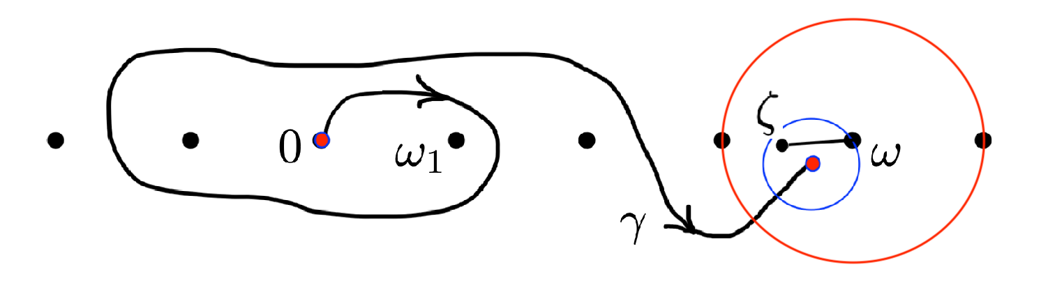
Figure 4: Analytic continuation along $\gamma$, for $\zeta$ near $\omega$.

The space $\widehat{\mathscr{R}}_{\Omega}^{\operatorname{simp}}$ (clearly a linear subspace of $\widehat{\mathscr{R}}_{\Omega}$) happens to be stable under convolution [23, § 6.13], hence $\mathbb{C}\delta\oplus\widehat{\mathscr{R}}_{\Omega}^{\operatorname{simp}}$ is a convolution subalgebra of $\mathbb{C}\delta\oplus\widehat{\mathscr{R}}_{\Omega}$ and, via the isomorphism $\mathscr{B}$, we obtain that $\widetilde{\mathscr{R}}_{\Omega}^{\operatorname{simp}}$ is a subalgebra of $\widetilde{\mathscr{R}}_{\Omega}\subset\mathbb{C}[[z^{-1}]]$ (trivially stable under $\frac{d\,}{dz}$ and containing $\mathbb{C}\{z^{-1}\}$).

2.6.3  In the situation described in Definition 2.8(i), the number $b$ and the holomorphic germ $\widehat{\psi}$ are uniquely determined and they depend linearly on $\widehat{\varphi}$; indeed,

$${\stackrel{{\scriptstyle\raisebox{-0.69318pt}{$\scriptscriptstyle\vee$}}}{{\psi}}}(\xi)\coloneqq\operatorname{cont}_{\gamma}\widehat{\varphi}(\omega+\xi)$$ (2.61)

can be viewed as function holomorphic in the universal cover of $\mathbb{D}_{|\omega_{1}|}^{*}$ and

$$b=\lim_{\xi\to 0}2\pi i\xi\,{\stackrel{{\scriptstyle\raisebox{-0.69318pt}{$\scriptscriptstyle\vee$}}}{{\psi}}}(\xi),\quad\widehat{\psi}(\xi)={\stackrel{{\scriptstyle\raisebox{-0.69318pt}{$\scriptscriptstyle\vee$}}}{{\psi}}}(\xi)-{\stackrel{{\scriptstyle\raisebox{-0.69318pt}{$\scriptscriptstyle\vee$}}}{{\psi}}}(e^{-2\pi i}\xi).$$ (2.62)

Moreover, being the difference of two branches of the analytic continuation of a simple $\Omega$-continuable germ shifted by an element of $\Omega$, $\widehat{\psi}$ is itself a simple $\Omega$-continuable germ. We can thus define an operator

$$\mathscr{A}^{\gamma}_{\omega}\colon\thinspace\mathbb{C}\delta\oplus\widehat{\mathscr{R}}_{\Omega}^{\operatorname{simp}}\to\mathbb{C}\delta\oplus\widehat{\mathscr{R}}_{\Omega}^{\operatorname{simp}}\enspace\text{such that}\enspace\mathscr{A}^{\gamma}_{\omega}(a\delta+\widehat{\varphi})=b\delta+\widehat{\psi}$$ (2.63)

for $a\in\mathbb{C}$ and $\widehat{\varphi}\in\widehat{\mathscr{R}}_{\Omega}^{\operatorname{simp}}$, with $b$ and $\widehat{\psi}$ determined by (2.59). This operator, which annihilates $\mathbb{C}\delta$ and encodes the singularity at $\omega$ obtained by analytic continuation along the path $\gamma$, is called an alien operator. Its counterpart $\mathscr{B}^{-1}\circ\mathscr{A}^{\gamma}_{\omega}\circ\mathscr{B}$ in the space of simple $\Omega$-resurgent series is denoted by the same symbol

$$\mathscr{A}^{\gamma}_{\omega}\colon\thinspace\widetilde{\mathscr{R}}_{\Omega}^{\operatorname{simp}}\to\widetilde{\mathscr{R}}_{\Omega}^{\operatorname{simp}}.$$ (2.64)

From the definition and (2.25), it is easy to compute the commutator

$$\Big{[}\frac{d\,}{dz},\mathscr{A}^{\gamma}_{\omega}\Big{]}=\omega\mathscr{A}^{\gamma}_{\omega}.$$ (2.65)

Two families of alien operators are particularly interesting:

Definition 2.9.

Let $\omega\in\Omega^{*}$. We define

$$\Delta^{+}_{\omega},\;\Delta_{\omega}\colon\thinspace\widetilde{\mathscr{R}}^{\operatorname{simp}}_{\Omega}\to\widetilde{\mathscr{R}}^{\operatorname{simp}}_{\Omega}$$ (2.66)

by the formulas

$$\Delta^{+}_{\omega}\coloneqq\mathscr{A}_{\omega}^{\gamma(+,\cdots,+)},\quad\Delta_{\omega}\coloneqq\sum\limits_{\varepsilon\in\{+,-\}^{r-1}}\frac{p(\varepsilon)!q(\varepsilon)!}{r!}\mathscr{A}_{\omega}^{\gamma(\varepsilon)},$$ (2.67)

with notations as follows:

1. among the two generators of $\Omega$ we have chosen $\omega_{1}$ so that $\omega=r\omega_{1}$ with $r\in\mathbb{Z}_{\geqslant 1}$,

2. for any $\varepsilon=(\varepsilon_{1},\cdots,\varepsilon_{r-1})\in\{+,-\}^{r-1}$ we have denoted by $p(\varepsilon)$ and $q(\varepsilon)=r-1-p(\varepsilon)$ numbers of symbols ‘$+$’ and ‘$-$’, and by $\gamma(\varepsilon)$ a path that follows the line-segment $[0,(r-\frac{1}{4})\omega]$ except that it circumvents $j\omega$ to the right if $\varepsilon_{j}=+$ and to the left if $\varepsilon_{j}=-$ for any $j\in\{1,\ldots,r-1\}$ (see Figure 5).

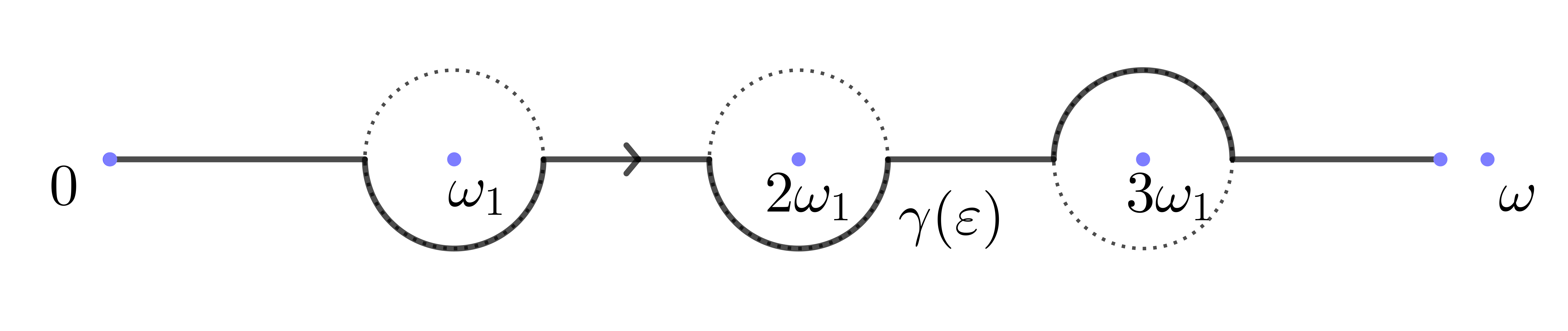
Figure 5: An example of a path $\gamma(\varepsilon)$, with $r=4$ and $\varepsilon=(+,+,-).$

One can prove that

$$\Delta^{+}_{\omega}(\widetilde{\varphi}_{1}\widetilde{\varphi}_{2})=(\Delta^{+}_{\omega}\widetilde{\varphi}_{1})\widetilde{\varphi}_{2}+\sum\limits_{\begin{subarray}{c}\omega=\omega_{1}+\omega_{2}\\ \omega_{1},\omega_{2}\in\Omega\,\cap\,]0,\omega[\end{subarray}}(\Delta^{+}_{\omega_{1}}\widetilde{\varphi}_{1})(\Delta^{+}_{\omega_{2}}\widetilde{\varphi}_{2})+\widetilde{\varphi}_{1}(\Delta^{+}_{\omega}\widetilde{\varphi}_{2}).$$ (2.68)

The reason why J. Écalle introduced the slightly more complicated definition of $\Delta_{\omega}$ was the desire to have a family of derivations of the algebra $\widetilde{\mathscr{R}}_{\Omega}^{\operatorname{simp}}$:

Theorem 2.10 ([23, Theorems 6.88 and 6.91]).

Let $\omega\in\Omega^{*}$. For any $\widetilde{\varphi}_{1}$ and $\widetilde{\varphi}_{2}\in\widetilde{\mathscr{R}}^{\operatorname{simp}}_{\Omega}$, we have the Leibniz rule

$$\Delta_{\omega}(\widetilde{\varphi}_{1}\widetilde{\varphi}_{2})=(\Delta_{\omega}\widetilde{\varphi}_{1})\widetilde{\varphi}_{2}+\widetilde{\varphi}_{1}(\Delta_{\omega}\widetilde{\varphi}_{2}).$$ (2.69)

Furthermore, if $\widetilde{\varphi},\widetilde{\psi},\widetilde{\chi}\in\widetilde{\mathscr{R}}^{\operatorname{simp}}_{\Omega}$, $\widetilde{\chi}$ has no constant term and $H(t)\in\mathbb{C}\{t\}$, then

$$\widetilde{\psi}\circ(id+\widetilde{\varphi})\in\widetilde{\mathscr{R}}_{\Omega}^{\operatorname{simp}},\quad H\circ\widetilde{\chi}\in\widetilde{\mathscr{R}}_{\Omega}^{\operatorname{simp}}$$ (2.70)

$$\Delta_{\omega}(\widetilde{\psi}\circ(id+\widetilde{\varphi})) =(\partial\widetilde{\psi})\circ(id+\widetilde{\varphi})\cdot\Delta_{\omega}\widetilde{\varphi}+e^{-\omega\widetilde{\varphi}}\cdot(\Delta_{\omega}\widetilde{\psi})\circ(id+\widetilde{\varphi})$$ (2.71)

$$\Delta_{\omega}(H\circ\widetilde{\chi}) =(\frac{dH}{dt}\circ\widetilde{\chi})\cdot\Delta_{\omega}\widetilde{\chi}$$ (2.72)

(alien chain rule).

Apart from the commutation rule with the natural derivation

$$\Big{[}\frac{d\,}{dz},\Delta_{\omega}\Big{]}=\omega\Delta_{\omega},$$ (2.73)

there are no other relations between these operators and $\frac{d\,}{dz}$ or among themselves; they are called Écalle’s alien derivations.

2.7 Extension to more general singularities

Returning to the general $\Omega$-continuable germs of $\widehat{\mathscr{R}}_{\Omega}=\mathscr{O}(\mathcal{S}_{\Omega})$, if one wants to deal with arbitrary kinds of singularities and not just simple singularities, one may fix once for all a generator $\omega_{1}\in\mathbb{C}\setminus\mathbb{R}_{\leqslant 0}$ and consider the quotient space

$$\raisebox{0.43057pt}{${\stackrel{{\scriptstyle\raisebox{-0.69318pt}{$\scriptscriptstyle\bigtriangledown$}}}{{\mathscr{R}}}}$}_{\Omega}\coloneqq\mathscr{O}(\mathcal{S}_{\Omega}^{*})/\mathscr{O}(\mathcal{S}_{\Omega})$$

where, with reference to (2.57), we identify a function $\raisebox{-0.99025pt}{${\stackrel{{\scriptstyle\raisebox{-0.69318pt}{$\scriptscriptstyle\vee$}}}{{\varphi}}}$}\in\mathscr{O}(\mathcal{S}_{\Omega}^{*})$ with a holomorphic germ at $\frac{1}{4}\omega_{1}$ that has analytic continuation along any path of $\mathscr{P}_{\Omega}^{*}$, and we view $\mathscr{O}(\mathcal{S}_{\Omega})$ as the subspace of those germs that have analytic continuation in $\mathbb{D}_{|\omega_{1}|}$ (whereas the other elements of $\mathscr{O}(\mathcal{S}_{\Omega}^{*})$ are singular at $0$). Using the notation

$$\raisebox{-0.99025pt}{${\stackrel{{\scriptstyle\raisebox{-0.69318pt}{$\scriptscriptstyle\vee$}}}{{\varphi}}}$}\in\mathscr{O}(\mathcal{S}_{\Omega}^{*})\mapsto\raisebox{-0.99025pt}{${\stackrel{{\scriptstyle\raisebox{-0.69318pt}{$\scriptscriptstyle\triangledown$}}}{{\varphi}}}$}=\operatorname{sing}_{0}(\raisebox{-0.99025pt}{${\stackrel{{\scriptstyle\raisebox{-0.69318pt}{$\scriptscriptstyle\vee$}}}{{\varphi}}}$})\in\raisebox{0.43057pt}{${\stackrel{{\scriptstyle\raisebox{-0.69318pt}{$\scriptscriptstyle\bigtriangledown$}}}{{\mathscr{R}}}}$}_{\Omega}$$

for the canonical projection, we call ${\stackrel{{\scriptstyle\raisebox{-0.69318pt}{$\scriptscriptstyle\triangledown$}}}{{\varphi}}}$ an $\Omega$-continuable singularity and ${\stackrel{{\scriptstyle\raisebox{-0.69318pt}{$\scriptscriptstyle\vee$}}}{{\varphi}}}$ a major of ${\stackrel{{\scriptstyle\raisebox{-0.69318pt}{$\scriptscriptstyle\triangledown$}}}{{\varphi}}}$. The minor of ${\stackrel{{\scriptstyle\raisebox{-0.69318pt}{$\scriptscriptstyle\triangledown$}}}{{\varphi}}}$ is defined as the function

$$\widehat{\varphi}(\zeta)=\operatorname{min}\raisebox{-0.99025pt}{${\stackrel{{\scriptstyle\raisebox{-0.69318pt}{$\scriptscriptstyle\triangledown$}}}{{\varphi}}}$}(\zeta)=\raisebox{-0.99025pt}{${\stackrel{{\scriptstyle\raisebox{-0.69318pt}{$\scriptscriptstyle\vee$}}}{{\varphi}}}$}(\zeta)-\raisebox{-0.99025pt}{${\stackrel{{\scriptstyle\raisebox{-0.69318pt}{$\scriptscriptstyle\vee$}}}{{\varphi}}}$}(e^{-2\pi i}\zeta)\in\mathscr{O}(\mathcal{S}_{\Omega}^{*})\quad\text{for any major $\raisebox{-0.99025pt}{${\stackrel{{\scriptstyle\raisebox{-0.69318pt}{$\scriptscriptstyle\vee$}}}{{\varphi}}}$}$ of~$\raisebox{-0.99025pt}{${\stackrel{{\scriptstyle\raisebox{-0.69318pt}{$\scriptscriptstyle\triangledown$}}}{{\varphi}}}$}$.}$$

One should think of the elements of $\raisebox{0.43057pt}{${\stackrel{{\scriptstyle\raisebox{-0.69318pt}{$\scriptscriptstyle\bigtriangledown$}}}{{\mathscr{R}}}}$}_{\Omega}$ as of singularities at the origin, among which simple singularities at $0$ are obtained from the embedding

$$\Phi\colon\thinspace a\delta+\widehat{\varphi}\in\mathbb{C}\delta\oplus\widehat{\mathscr{R}}_{\Omega}\mapsto\raisebox{-0.99025pt}{${\stackrel{{\scriptstyle\raisebox{-0.69318pt}{$\scriptscriptstyle\triangledown$}}}{{\varphi}}}$}=\operatorname{sing}_{0}\Big{(}\frac{a}{2\pi i\zeta}+\widehat{\varphi}(\zeta)\frac{\log\zeta}{2\pi i}\Big{)}\in\raisebox{0.43057pt}{${\stackrel{{\scriptstyle\raisebox{-0.69318pt}{$\scriptscriptstyle\bigtriangledown$}}}{{\mathscr{R}}}}$}_{\Omega}.$$ (2.74)

The formalism of $\Omega$-continuable singularities will appear as an extension of $\Omega$-continuable germs. It turns out that there exists a commutative convolution law in $\raisebox{0.43057pt}{${\stackrel{{\scriptstyle\raisebox{-0.69318pt}{$\scriptscriptstyle\bigtriangledown$}}}{{\mathscr{R}}}}$}_{\Omega}$ for which $\Phi$ is an algebra homomorphism.

An elementary example of $\Omega$-continuable singularity at $0$ is given by

$$\raisebox{0.86108pt}{${\stackrel{{\scriptstyle\raisebox{-0.60275pt}{$\scriptscriptstyle\triangledown$}}}{{I}}}$}_{\nu}\coloneqq\operatorname{sing}_{0}(\raisebox{0.86108pt}{${\stackrel{{\scriptstyle\raisebox{-0.60275pt}{$\scriptscriptstyle\vee$}}}{{I}}}$}_{\nu}),\quad\raisebox{0.86108pt}{${\stackrel{{\scriptstyle\raisebox{-0.60275pt}{$\scriptscriptstyle\vee$}}}{{I}}}$}_{\nu}(\zeta)\coloneqq\frac{e^{i\pi\nu}\Gamma(1-\nu)}{2\pi i}\zeta^{\nu-1}\quad\text{for $\nu\in\mathbb{C}\setminus\mathbb{Z}_{\geqslant 1}$.}$$ (2.75)

Its minor is $\widehat{I}_{\nu}(\zeta)\coloneqq\zeta^{\nu-1}/\Gamma(\nu)$ (which is $0$ if $\nu\in\mathbb{Z}_{\leqslant 0}$). The singularity $\raisebox{0.86108pt}{${\stackrel{{\scriptstyle\raisebox{-0.60275pt}{$\scriptscriptstyle\triangledown$}}}{{I}}}$}_{\nu}$ is not a simple singularity at $0$ unless $\nu=0$, in which case we find $\raisebox{0.86108pt}{${\stackrel{{\scriptstyle\raisebox{-0.60275pt}{$\scriptscriptstyle\triangledown$}}}{{I}}}$}_{0}=\Phi(\delta)$. For $\nu\notin\mathbb{Z}$ we use the principal branch of $\zeta^{\nu-1}$, which we view as element of $\mathscr{O}(\mathcal{S}_{\Omega}^{*})$ by declaring that $\arg(\frac{1}{4}\omega_{1})\in(-\pi,\pi)$. If we extend the family $\big{(}\raisebox{0.86108pt}{${\stackrel{{\scriptstyle\raisebox{-0.60275pt}{$\scriptscriptstyle\triangledown$}}}{{I}}}$}_{\nu}\big{)}$ to all $\nu\in\mathbb{C}$ by

$$\raisebox{0.86108pt}{${\stackrel{{\scriptstyle\raisebox{-0.60275pt}{$\scriptscriptstyle\vee$}}}{{I}}}$}_{n}(\zeta)\coloneqq\frac{\zeta^{n-1}}{\Gamma(n)}\frac{\log\zeta}{2\pi i}\quad\text{for $n\in\mathbb{Z}_{\geqslant 1}$,}$$

then the aforementioned convolution law of $\raisebox{0.43057pt}{${\stackrel{{\scriptstyle\raisebox{-0.69318pt}{$\scriptscriptstyle\bigtriangledown$}}}{{\mathscr{R}}}}$}_{\Omega}$ satisfies $\raisebox{0.86108pt}{${\stackrel{{\scriptstyle\raisebox{-0.60275pt}{$\scriptscriptstyle\triangledown$}}}{{I}}}$}_{\nu_{1}}*\raisebox{0.86108pt}{${\stackrel{{\scriptstyle\raisebox{-0.60275pt}{$\scriptscriptstyle\triangledown$}}}{{I}}}$}_{\nu_{2}}=\raisebox{0.86108pt}{${\stackrel{{\scriptstyle\raisebox{-0.60275pt}{$\scriptscriptstyle\triangledown$}}}{{I}}}$}_{\nu_{1}+\nu_{2}}$. More generally, for any $\nu\in\mathbb{C}$ such that $\mathop{\Re e}\nolimits\nu>0$, there is an embedding

$$\widehat{\varphi}\in\zeta^{\nu-1}\mathbb{C}\{\zeta\}\cap\mathscr{O}(\mathcal{S}_{\Omega}^{*})\mapsto\mbox{}^{\flat}\hskip-0.8pt\widehat{\varphi}\in\raisebox{0.43057pt}{${\stackrel{{\scriptstyle\raisebox{-0.69318pt}{$\scriptscriptstyle\bigtriangledown$}}}{{\mathscr{R}}}}$}_{\Omega}$$

such that $\operatorname{min}\big{(}\mbox{}^{\flat}\hskip-0.8pt\widehat{\varphi}\big{)}=\widehat{\varphi}$ and $\mbox{}^{\flat}\hskip-0.8pt\widehat{\varphi}_{1}*\mbox{}^{\flat}\hskip-0.8pt\widehat{\varphi}_{2}=\mbox{}^{\flat}\hskip-0.8pt\big{(}\widehat{\varphi}_{1}*\widehat{\varphi}_{2}\big{)}$, where $\widehat{\varphi}_{1}*\widehat{\varphi}_{2}$ is the convolution of integrable minors defined by (2.5), namely

$$\nu\notin\mathbb{Z}\enspace\Longrightarrow\enspace\mbox{}^{\flat}\hskip-0.8pt\widehat{\varphi}=\operatorname{sing}_{0}\Big{(}\frac{\widehat{\varphi}(\zeta)}{1-e^{-2\pi i\nu}}\Big{)},\quad\nu\in\mathbb{Z}_{\geqslant 1}\enspace\Longrightarrow\enspace\mbox{}^{\flat}\hskip-0.8pt\widehat{\varphi}=\operatorname{sing}_{0}\Big{(}\widehat{\varphi}(\zeta)\frac{\log\zeta}{2\pi i}\Big{)}$$

(note that (2.74) can be rewritten $\Phi(a\delta+\widehat{\varphi})=a\raisebox{0.86108pt}{${\stackrel{{\scriptstyle\raisebox{-0.60275pt}{$\scriptscriptstyle\triangledown$}}}{{I}}}$}_{0}+\mbox{}^{\flat}\hskip-0.8pt\widehat{\varphi}$).

We can now extend Definition 2.9 and define operators of $\raisebox{0.43057pt}{${\stackrel{{\scriptstyle\raisebox{-0.69318pt}{$\scriptscriptstyle\bigtriangledown$}}}{{\mathscr{R}}}}$}_{\Omega}$ that measure singularities at certain “boundary points” of $\mathcal{S}_{\Omega}$. These new operators $\Delta^{+}_{\widetilde{\omega}}$ and $\Delta_{\widetilde{\omega}}$ will be indexed by all ${\widetilde{\omega}}\in{\widetilde{\Omega}}^{*}$, where ${\widetilde{\Omega}}^{*}$ is the lift $\pi^{-1}(\Omega^{*})$ of $\Omega^{*}$ to the Riemann surface of the logarithm $\pi\colon\thinspace\widetilde{\mathbb{C}}\to\mathbb{C}^{*}$, and they will boil down to the previous $\Delta^{+}_{\omega}$ and $\Delta_{\omega}$ in the case of simple singularities in the sense that

$$\Delta_{\widetilde{\omega}}^{+}\circ\Phi=\Phi\circ\Delta_{\omega}^{+},\quad\Delta_{\widetilde{\omega}}\circ\Phi=\Phi\circ\Delta_{\omega}.$$

To proceed, we write ${\widetilde{\omega}}=e^{i\pi N}r\omega_{1}$ with $r\in\mathbb{Z}_{\geqslant 1}$ and $N\in\mathbb{Z}$ and let

$$\Delta_{\widetilde{\omega}}^{+}\raisebox{-0.99025pt}{${\stackrel{{\scriptstyle\raisebox{-0.69318pt}{$\scriptscriptstyle\triangledown$}}}{{\varphi}}}$}\coloneqq\operatorname{sing}_{0}\!\Big{(}(\operatorname{cont}_{\widetilde{\gamma}(+,\cdots,+)}\operatorname{min}\raisebox{-0.99025pt}{${\stackrel{{\scriptstyle\raisebox{-0.69318pt}{$\scriptscriptstyle\triangledown$}}}{{\varphi}}}$})({\widetilde{\omega}}+\zeta)\Big{)}$$

$$\Delta_{\widetilde{\omega}}\raisebox{-0.99025pt}{${\stackrel{{\scriptstyle\raisebox{-0.69318pt}{$\scriptscriptstyle\triangledown$}}}{{\varphi}}}$}\coloneqq\sum\limits_{\varepsilon\in\{+,-\}^{r-1}}\frac{p(\varepsilon)!q(\varepsilon)!}{r!}\operatorname{sing}_{0}\!\Big{(}(\operatorname{cont}_{\widetilde{\gamma}(\varepsilon)}\operatorname{min}\raisebox{-0.99025pt}{${\stackrel{{\scriptstyle\raisebox{-0.69318pt}{$\scriptscriptstyle\triangledown$}}}{{\varphi}}}$})({\widetilde{\omega}}+\zeta)\Big{)}$$

where $\widetilde{\gamma}(\varepsilon)$ goes from $\frac{1}{4}\omega_{1}$ to $\frac{1}{4}e^{i\pi N}\omega_{1}$ turning around the origin ($N$ half-turns) and follows the line-segment $[\frac{1}{4}e^{i\pi N}\omega_{1},(r-\frac{1}{4})e^{i\pi N}\omega_{1}]$ except that it circumvents $j\omega$ to the right if $\varepsilon_{j}=+$ and to the left if $\varepsilon_{j}=-$ for any $j\in\{1,\ldots,r-1\}$, and we add a half-turn around $\omega$ from $(r-\frac{1}{4})e^{i\pi N}\omega_{1}$ to $(r+\frac{1}{4})e^{i\pi N}\omega_{1}$ if $N$ is even (so that in all cases $\widetilde{\gamma}(\varepsilon)$ ends at $\omega+\frac{1}{4}\omega_{1}$, where $\omega$ is the projection of ${\widetilde{\omega}}$ in $\mathbb{C}^{*}$, and there is a natural way of viewing $(\operatorname{cont}_{\widetilde{\gamma}(\varepsilon)}\operatorname{min}\raisebox{-0.99025pt}{${\stackrel{{\scriptstyle\raisebox{-0.69318pt}{$\scriptscriptstyle\triangledown$}}}{{\varphi}}}$})({\widetilde{\omega}}+\zeta)$ as element of $\mathscr{O}(\mathcal{S}_{\Omega}^{*})$). See Figure 6.

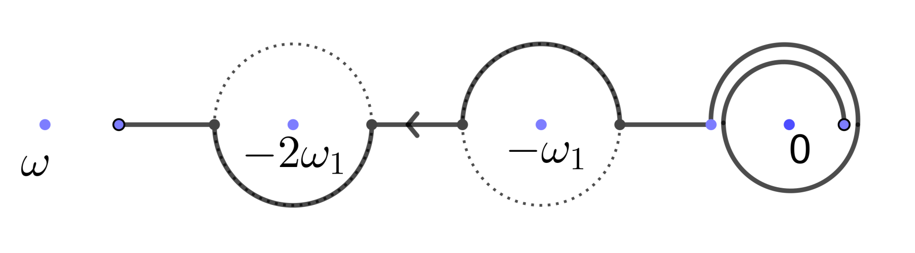
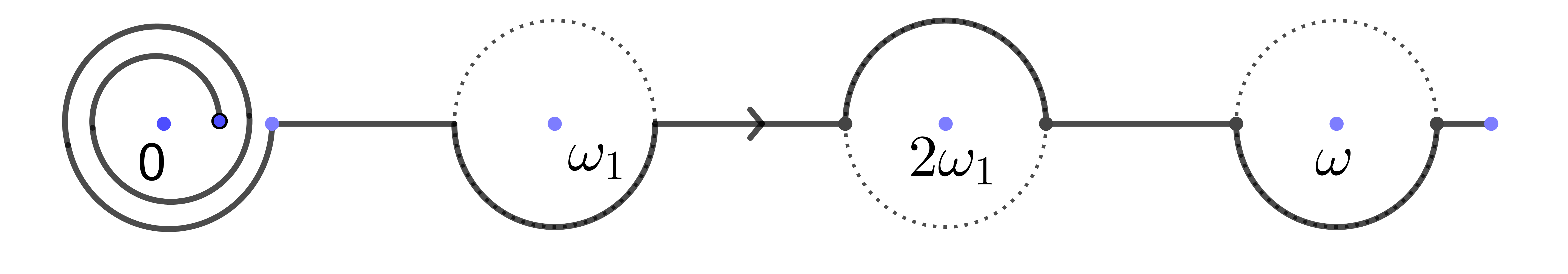
Figure 6: Examples of path $\widetilde{\gamma}(\varepsilon)$, with $r=3$, $\varepsilon=(+,-)$. Left: $N=3$. Right: $N=4$. In all cases $\gamma(0)=\frac{1}{4}\omega_{1}$ and $\gamma(1)=\omega+\frac{1}{4}\omega_{1}$

One can view $\mathbb{C}\delta\oplus\widehat{\mathscr{R}}_{\Omega}^{\operatorname{simp}}$ as the largest subspace of $\mathbb{C}\delta\oplus\widehat{\mathscr{R}}_{\Omega}$ whose image by $\Phi$ is stable under all operators $\Delta_{\widetilde{\omega}}$.

2.8 Resurgence in the Airy equation

In Section 2.5 we have introduced various formal series in relation with the Airy equation; in view of (2.35) and (2.46),

$$\widehat{A}(\zeta)=\tfrac{\zeta^{-\frac{1}{6}}}{\Gamma(\frac{5}{6})}(1-\tfrac{\zeta}{2})^{-\frac{1}{6}}\quad\text{and}\quad\widehat{A}_{+}(\zeta)=\tfrac{\zeta^{-\frac{1}{6}}}{\Gamma(\frac{5}{6})}(1+\tfrac{\zeta}{2})^{-\frac{1}{6}}$$

may be considered as integrable $2\mathbb{Z}$-continuable minors (that are not regular at the origin), and (2.37) and (2.47) can be rewritten

$$\widehat{B}=\widehat{I}_{1/6}*\widehat{A},\enspace\widehat{B}_{+}=\widehat{I}_{1/6}*\widehat{A}_{+},\\[4.30554pt] \text{whence}\quad\mbox{}^{\flat}\hskip-0.8pt\widehat{B}=\raisebox{0.86108pt}{${\stackrel{{\scriptstyle\raisebox{-0.60275pt}{$\scriptscriptstyle\triangledown$}}}{{I}}}$}_{1/6}*\mbox{}^{\flat}\hskip-0.8pt\!\widehat{A},\enspace\mbox{}^{\flat}\hskip-0.8pt\widehat{B}_{+}=\raisebox{0.86108pt}{${\stackrel{{\scriptstyle\raisebox{-0.60275pt}{$\scriptscriptstyle\triangledown$}}}{{I}}}$}_{1/6}*\mbox{}^{\flat}\hskip-0.8pt\!\widehat{A}_{+}\in\raisebox{0.43057pt}{${\stackrel{{\scriptstyle\raisebox{-0.69318pt}{$\scriptscriptstyle\bigtriangledown$}}}{{\mathscr{R}}}}$}_{2\mathbb{Z}}.$$

Applying the above recipe and taking care of identifying the right branches of the analytic continuation, we get

$$\Delta_{2e^{i0}}\mbox{}^{\flat}\hskip-0.8pt\!\widehat{A}=\operatorname{sing}_{0}\bigg{(}\frac{(2+\zeta)^{-\frac{1}{6}}}{\Gamma(\frac{5}{6})}\Big{(}\frac{e^{i\pi}\zeta}{2}\Big{)}^{-\frac{1}{6}}\bigg{)}=e^{-i\pi/6}\operatorname{sing}_{0}\big{(}\widehat{A}_{+}(\zeta)\big{)}\\[4.30554pt] =e^{-i\pi/6}(1-e^{2\pi i/6})\,\mbox{}^{\flat}\hskip-0.8pt\!\widehat{A}_{+}=-i\,\mbox{}^{\flat}\hskip-0.8pt\!\widehat{A}_{+}$$

and, similarly,

$$\Delta_{2e^{i\pi}}\mbox{}^{\flat}\hskip-0.8pt\!\widehat{A}_{+}=\operatorname{sing}_{0}\bigg{(}\frac{\big{(}(2e^{i\pi})(1-\frac{\zeta}{2})\big{)}^{-\frac{1}{6}}}{\Gamma(\frac{5}{6})}\Big{(}\frac{\zeta}{2}\Big{)}^{-\frac{1}{6}}\bigg{)}=e^{-i\pi/6}\operatorname{sing}_{0}\big{(}\widehat{A}(\zeta)\big{)}\\ =-i\,\mbox{}^{\flat}\hskip-0.8pt\!\widehat{A}.$$

Since $\Delta_{2e^{i0}}$ and $\Delta_{2e^{i\pi}}$ are derivations that annihilate $\raisebox{0.86108pt}{${\stackrel{{\scriptstyle\raisebox{-0.60275pt}{$\scriptscriptstyle\triangledown$}}}{{I}}}$}_{1/6}$, it follows that

$$\Delta_{2e^{i0}}\mbox{}^{\flat}\hskip-0.8pt\widehat{B}=-i\,\mbox{}^{\flat}\hskip-0.8pt\widehat{B}_{+},\quad\Delta_{2e^{i\pi}}\mbox{}^{\flat}\hskip-0.8pt\widehat{B}_{+}=-i\,\mbox{}^{\flat}\hskip-0.8pt\widehat{B}\quad\text{in the algebra~$\raisebox{0.43057pt}{${\stackrel{{\scriptstyle\raisebox{-0.69318pt}{$\scriptscriptstyle\bigtriangledown$}}}{{\mathscr{R}}}}$}_{2\mathbb{Z}}$,}$$

which boils down to

$$\Delta_{2}\widehat{B}=-i\,\widehat{B}_{+},\quad\Delta_{-2}\widehat{B}_{+}=-i\,\widehat{B}\quad\text{in}\enspace\mathbb{C}\delta\oplus\mathscr{R}_{2\mathbb{Z}}^{\operatorname{simp}}.$$

Finally, since $\widetilde{B}=z^{-1}\widetilde{\psi}$ and $\widetilde{B}_{+}=z^{-1}\widetilde{\varphi}$, we can rewrite this as

$$\widetilde{\psi},\widetilde{\varphi}\in\widetilde{\mathscr{R}}_{2\mathbb{Z}},\quad\Delta^{+}_{2}\widetilde{\psi}=\Delta_{2}\widetilde{\psi}=-i\widetilde{\varphi},\quad\Delta^{+}_{-2}\widetilde{\varphi}=\Delta_{-2}\widetilde{\varphi}=-i\widetilde{\psi}$$ (2.76)

(using the fact that $\Delta^{+}_{\omega}=\Delta_{\omega}$ when $\omega$ is a generator of $\Omega$). On the other hand,

$$\omega\in 2\mathbb{Z}^{*}\setminus\{2\}\enspace\Longrightarrow\enspace\Delta_{\omega}\widetilde{\psi}=0,\qquad\omega\in 2\mathbb{Z}^{*}\setminus\{-2\}\enspace\Longrightarrow\enspace\Delta_{\omega}\widetilde{\varphi}=0.$$ (2.77)

2.9 Simple $\Omega$-resurgent transseries

We now explain the interplay between Borel-Laplace summation and alien calculus in the case of simple $\Omega$-resurgent series (but much of what follows can be adapted to the case of more general singularities).

2.9.1  We first fix $\omega_{1}\in\mathbb{C}^{*}$ and $\Omega=\mathbb{Z}\,\omega_{1}$ as in Sections 2.6–2.7, and set

$$d\coloneqq\mathbb{R}_{\geqslant 0}\,\omega_{1},\quad\Omega^{+}\coloneqq d\cap\Omega^{*}=\{m\,\omega_{1}\mid m\in\mathbb{Z}_{\geqslant 1}\}.$$ (2.78)

Definition 2.11.

We call simple $\Omega$-resurgent transseries any expression of the form

$$\widetilde{\Psi}=\sum\limits_{m\geqslant 0}e^{-m\,\omega_{1}z}\widetilde{\psi}_{m}(z)$$

where $(\widetilde{\psi}_{m})_{m\geqslant 0}$ is a sequence in $\widetilde{\mathscr{R}}_{\Omega}^{\operatorname{simp}}$.

The space of all simple $\Omega$-resurgent transseries can be viewed as a completed graded algebra

$$\widetilde{\mathscr{R}}_{\Omega}^{\operatorname{simp}}[[e^{-\omega_{1}z}]]=\bigoplus_{m\geqslant 0}^{\wedge}e^{-m\,\omega_{1}z}\widetilde{\mathscr{R}}_{\Omega}^{\operatorname{simp}},$$

i.e. we can manipulate infinite sums thanks to the notion of formal convergence induced by the $m$-grading.

Theorem 2.12 ([23, p. 226]).

Consider the two operators of $\widetilde{\mathscr{R}}_{\Omega}^{\operatorname{simp}}[[e^{-\omega_{1}z}]]$ defined by

$${{\Delta}}\hskip-6.00006pt\raisebox{1.59302pt}{\leavevmode\resizebox{2.58334pt}{}{$\mathrm{/}$}}\hskip 3.99994pt{}_{d}\coloneqq\sum\limits_{\omega\in\Omega^{+}}e^{-\omega z}\Delta_{\omega},\quad{{\Delta}}\hskip-6.00006pt\raisebox{1.59302pt}{\leavevmode\resizebox{2.58334pt}{}{$\mathrm{/}$}}\hskip 3.99994pt{}_{d}^{+}\coloneqq\mathop{\hbox{{\rm Id}}}\nolimits+\sum\limits_{\omega\in\Omega^{+}}e^{-\omega z}\Delta_{\omega}^{+}$$ (2.79)

with the convention $\Delta_{\omega}(\sum e^{-m\,\omega_{1}z}\widetilde{\psi}_{m})\coloneqq\sum e^{-m\,\omega_{1}z}\Delta_{\omega}\widetilde{\psi}_{m}$ and similarly for $\Delta_{\omega}^{+}$. Then

(i) ${{\Delta}}\hskip-6.00006pt\raisebox{1.59302pt}{\leavevmode\resizebox{2.58334pt}{}{$\mathrm{/}$}}\hskip 3.99994pt{}_{d}$ is a derivation that commutes with the natural derivation $\frac{d\,}{dz}$;

(ii) ${{\Delta}}\hskip-6.00006pt\raisebox{1.59302pt}{\leavevmode\resizebox{2.58334pt}{}{$\mathrm{/}$}}\hskip 3.99994pt{}_{d}^{+}$ is an algebra automorphism that commutes with $\frac{d\,}{dz}$;

(iii) moreover,

$${{\Delta}}\hskip-6.00006pt\raisebox{1.59302pt}{\leavevmode\resizebox{2.58334pt}{}{$\mathrm{/}$}}\hskip 3.99994pt{}_{d}^{+}=\exp({{\Delta}}\hskip-6.00006pt\raisebox{1.59302pt}{\leavevmode\resizebox{2.58334pt}{}{$\mathrm{/}$}}\hskip 3.99994pt{}_{d})=\sum\limits_{s\geqslant 0}\frac{1}{s!}\left({{\Delta}}\hskip-6.00006pt\raisebox{1.59302pt}{\leavevmode\resizebox{2.58334pt}{}{$\mathrm{/}$}}\hskip 3.99994pt{}_{d}\right)^{s}.$$ (2.80)

The operator ${{\Delta}}\hskip-6.00006pt\raisebox{1.59302pt}{\leavevmode\resizebox{2.58334pt}{}{$\mathrm{/}$}}\hskip 3.99994pt{}_{d}$ is called the symbolic Stokes infinitesimal generator for the direction $d$ and the operator ${{\Delta}}\hskip-6.00006pt\raisebox{1.59302pt}{\leavevmode\resizebox{2.58334pt}{}{$\mathrm{/}$}}\hskip 3.99994pt{}_{d}^{+}$ is called the symbolic Stokes automorphism for the direction $d$. Note that the right-hand side of (2.80) makes sense because ${{\Delta}}\hskip-6.00006pt\raisebox{1.59302pt}{\leavevmode\resizebox{2.58334pt}{}{$\mathrm{/}$}}\hskip 3.99994pt{}_{d}$ increases the $m$-grading. This relation implies that the family of operators $(\Delta_{m\omega_{1}}^{+})_{m\geqslant 1}$ can be expressed in terms of the family $(\Delta_{m\omega_{1}})_{m\geqslant 1}$,

$$\Delta_{\omega_{1}}^{+}=\Delta_{\omega_{1}},\quad\Delta_{2\omega_{1}}^{+}=\Delta_{2\omega_{1}}+\tfrac{1}{2!}\Delta_{\omega_{1}}\circ\Delta_{\omega_{1}},\\[4.30554pt] \Delta_{3\omega_{1}}^{+}=\Delta_{3\omega_{1}}+\tfrac{1}{2!}(\Delta_{2\omega_{1}}\circ\Delta_{\omega_{1}}+\Delta_{\omega_{1}}\circ\Delta_{2\omega_{1}})+\tfrac{1}{3!}\Delta_{\omega_{1}}\circ\Delta_{\omega_{1}}\circ\Delta_{\omega_{1}},\quad\text{etc.}$$

and vice versa. The commutation rules (2.65) and (2.73) show that each “homogeneous operator” $e^{-\omega z}\Delta_{\omega}^{+}$ or $e^{-\omega z}\Delta_{\omega}$ commutes with $\frac{d\,}{dz}$.

2.9.2  Let us write $\omega_{1}=|\omega_{1}|e^{i\theta^{*}}$ with $\theta^{*}\in\mathbb{R}$ and consider an interval $I=(\theta^{*}-\delta,\theta^{*}+\delta)$ of length $\leqslant\pi$. We will be interested in formal power series that are $1$-summable in the directions of $I\setminus\{\theta^{*}\}$, i.e. in the directions of

$$I_{R}\coloneqq(\theta^{*}-\delta,\theta^{*})\enspace\text{and}\enspace I_{L}\coloneqq(\theta^{*},\theta^{*}+\delta)$$ (2.81)

but not necessarily in the direction $\theta^{*}$; supposing them to be $\Omega$-resurgent our aim is to compare the action of the summation operators $\mathscr{S}^{I_{R}}$ and $\mathscr{S}^{I_{L}}$ defined by (2.18).

We thus give ourselves a locally bounded function $\alpha\colon\thinspace I_{R}\cup I_{L}\to\mathbb{R}_{\geqslant 0}$ and consider the space

$$\widetilde{\mathscr{R}}_{\Omega}^{\operatorname{simp}}(I,\alpha)\coloneqq\widetilde{\mathscr{R}}_{\Omega}^{\operatorname{simp}}\cap\big{(}\mathbb{C}\oplus\widetilde{\mathscr{N}}(I_{R},\alpha)\big{)}\cap\big{(}\mathbb{C}\oplus\widetilde{\mathscr{N}}(I_{L},\alpha)\big{)},$$

which is a subalgebra of $\mathbb{C}[[z^{-1}]]$. Note that

$$\mathscr{D}^{*}\coloneqq\mathscr{D}(I_{R},\alpha)\cap\mathscr{D}(I_{L},\alpha)$$

contains sectors bisected by $e^{-i\theta^{*}}\mathbb{R}_{\geqslant 0}$ of any opening $<\pi$, and is contained in the half-plane $\{\mathop{\Re e}\nolimits(ze^{i\theta_{*}})>0\}$, whence $e^{-\omega_{1}z}$ is exponentially small at infinity in that domain.

For any $\widetilde{\varphi}\in\widetilde{\mathscr{R}}_{\Omega}^{\operatorname{simp}}(I,\alpha)$, we want to compare the functions

$$\mathscr{S}^{I_{R}}\widetilde{\varphi}\in\mathscr{O}(\mathscr{D}(I_{R},\alpha))\quad\text{and}\quad\mathscr{S}^{I_{L}}\widetilde{\varphi}\in\mathscr{O}(\mathscr{D}(I_{L},\alpha)),$$

whose difference is exponentially small on $\mathscr{D}^{*}$. This is possible if we assume that $\Delta_{\omega}^{+}\widetilde{\varphi}\in\mathbb{C}\oplus\widetilde{\mathscr{N}}(I_{L},\alpha)$ for each $\omega\in\Omega^{+}$. The result is then

$$z\in\mathscr{D}^{*}\enspace\Longrightarrow\enspace\mathscr{S}^{I_{R}}\widetilde{\varphi}(z)=\mathscr{S}^{I_{L}}\widetilde{\varphi}(z)+\sum_{m=1}^{m_{*}}e^{-m\,\omega_{1}z}\mathscr{S}^{I_{L}}\Delta_{m\omega_{1}}^{+}\widetilde{\varphi}(z)+O(|e^{-\mu\,\omega_{1}z}|)$$ (2.82)

for any integer $m_{*}\geqslant 1$ and any real $\mu\in(m_{*},m_{*}+1)$.

The idea of the proof of (2.82) is to write $\mathscr{S}^{I_{R}}\widetilde{\varphi}(z)-\mathscr{S}^{I_{L}}\widetilde{\varphi}(z)$ as a Laplace-like integral on a contour $\Gamma_{\!\textrm{diff}}$ that can be decomposed in a sum of Hankel contours $\Gamma_{1},\Gamma_{2},\ldots$ as illustrated on Figure 7.

Figure 7: Decomposition of integration contour $\Gamma_{\!\textrm{diff}}$ for the computation of $\mathscr{S}^{I_{R}}\widetilde{\varphi}-\mathscr{S}^{I_{L}}\widetilde{\varphi}$.

It is sometimes possible to let $m_{*}$ tend to infinity and get

$$\mathscr{S}^{I_{R}}\widetilde{\varphi}(z)=\mathscr{S}^{I_{L}}\circ{{\Delta}}\hskip-6.00006pt\raisebox{1.59302pt}{\leavevmode\resizebox{2.58334pt}{}{$\mathrm{/}$}}\hskip 3.99994pt{}_{d}^{+}\widetilde{\varphi}(z)\quad\text{in restriction to $z\in\mathscr{D}^{*}$,}$$ (2.83)

where the right-hand side involves the action of the summation operator $\mathscr{S}^{I_{L}}$ on a simple $\Omega$-resurgent transseries, but this usually requires some justification. We will see two examples where (2.83) holds in Section 3 (in one case because there are only finitely many values of $m$ for which $\Delta_{m\omega_{1}}^{+}$ does not annihilate $\widetilde{\varphi}$, in the other case because both sides of (2.83) are solutions to the same ODE and it is thus easier to prove them equal).

Remark 2.13.

One can also make sense of (2.83) in the algebra $\widetilde{\mathscr{R}}_{\Omega}^{\operatorname{simp}}$ without summability assumption (i.e. without any exponential bound (2.8) or (2.8’)), at the price of replacing holomorphic functions on $\mathscr{D}^{*}$ by exponential evanescence classes [8].

Example 2.14.

For the formal series related to the Airy equation, we recall from Section 2.5 that

$$\widetilde{\psi}\in\mathbb{C}\oplus\widetilde{\mathscr{N}}(I_{0},0),\quad I_{0}=(-2\pi,0),\qquad\widetilde{\varphi}\in\mathbb{C}\oplus\widetilde{\mathscr{N}}(I_{\pi},0),\quad I_{\pi}=(-\pi,\pi)$$

and (2.76)–(2.77) yield

$${{\Delta}}\hskip-6.00006pt\raisebox{1.59302pt}{\leavevmode\resizebox{2.58334pt}{}{$\mathrm{/}$}}\hskip 3.99994pt{}_{\mathbb{R}_{\geqslant 0}}^{+}\widetilde{\psi}=\widetilde{\psi}-ie^{-2z}\widetilde{\varphi},\qquad{{\Delta}}\hskip-6.00006pt\raisebox{1.59302pt}{\leavevmode\resizebox{2.58334pt}{}{$\mathrm{/}$}}\hskip 3.99994pt{}_{\mathbb{R}_{\leqslant 0}}^{+}\widetilde{\varphi}=\widetilde{\varphi}-ie^{2z}\widetilde{\psi}.$$ (2.84)

Let us use $\theta^{*}=0$ or $-\pi$. For $z\in\widetilde{\mathbb{C}}$ (Riemann surface of the logarithm), we get

$$\arg z\in\big{(}\hskip-3.00003pt-\tfrac{\pi}{2},\tfrac{\pi}{2}\big{)} \enspace\Longrightarrow\enspace\mathscr{S}^{I_{0}}\widetilde{\psi}(z)=\mathscr{S}^{I_{0}}\widetilde{\psi}(e^{2\pi i}z)-ie^{-2z}\mathscr{S}^{I_{\pi}}\widetilde{\varphi}(z)$$ (2.85)

$$\arg z\in\big{(}\tfrac{\pi}{2},\tfrac{3\pi}{2}\big{)} \enspace\Longrightarrow\enspace\mathscr{S}^{I_{\pi}}\widetilde{\varphi}(e^{-2\pi i}z)=\mathscr{S}^{I_{\pi}}\widetilde{\varphi}(z)-ie^{2z}\mathscr{S}^{I_{0}}\widetilde{\psi}(z)$$ (2.86)

Indeed, (2.85) is obtained with $\theta^{*}=0$, $I_{R}=(-\delta,0)\subset I_{0}$ and $I_{L}=(0,\delta)\subset(2\pi+I_{0})\cap I_{\pi}$, using $\mathscr{S}^{2\pi+I_{0}}\widetilde{\psi}(z)=\mathscr{S}^{I_{0}}\widetilde{\psi}(e^{2\pi i}z)$ (cf. footnote 4). For (2.86): $\theta^{*}=-\pi$, $I_{R}\subset-2\pi+I_{\pi}$, $I_{L}\subset I_{\pi}\cap I_{0}$.

3 Resurgent analysis of the free energy in the double scaling limit

In this section we apply resurgence theory to the study of the free energy as obtained by Alim-Yau-Zhou’s double scaling limit ([3]). Following background and motivations from §1, we consider the second-order ordinary differential equation (1.5) derived from the holomorphic anomaly equations in their polynomial form. As shown in [3], the all-genus free energy

$$\mathcal{F}^{\hskip 0.52498pt\mathrm{s}}(\lambda_{s})=\sum_{g=2}^{\infty}a_{g}\lambda_{s}^{2(g-1)}$$

(cf. (1.3)) is the only solution to equation (1.5) in $\lambda_{s}^{2}\mathbb{C}[[\lambda_{s}^{2}]]$. More precisely, we have

Lemma 3.1.

The formal solutions to Equation (1.5) in $\mathbb{C}[[\lambda^{2}_{s}]]$ are the formal series

$$\sigma+\mathcal{F}^{\hskip 0.52498pt\mathrm{s}}(\lambda_{s}),\qquad\sigma\in\mathbb{C}.$$

To apply the resurgence theory to study $\mathcal{F}^{\hskip 0.52498pt\mathrm{s}}$, we first change the variable to $z=\frac{1}{3\lambda_{s}^{2}}$. From now on, we will systematically use the variable $z$ rather than $\lambda_{s}$. Then $\mathcal{F}^{\hskip 0.52498pt\mathrm{s}}$ becomes $\widetilde{g}(z)=\widetilde{g}(\frac{1}{3\lambda_{s}^{2}})=\mathcal{F}^{\hskip 0.52498pt\mathrm{s}}(\lambda_{s})$, i.e.

$$\widetilde{g}(z)\coloneqq\mathcal{F}^{\hskip 0.52498pt\mathrm{s}}((3z)^{-1/2})=\sum\limits_{g=2}^{\infty}3^{-(g-1)}a_{g}z^{-(g-1)}=\sum\limits_{n=1}^{\infty}b_{n}z^{-n},\qquad b_{n}\coloneqq 3^{-n}a_{n+1}.$$ (3.1)

Our change of variable changes the ODE (1.5) into

$$g^{\prime\prime}+(g^{\prime})^{2}+2g^{\prime}+\frac{5}{36}z^{-2}=0,$$ (3.2)

the formal solutions of which are thus $\sigma+\widetilde{g}(z)$, $\sigma\in\mathbb{C}$.

The proof of Theorem A will result from a succession of propositions to be found in Sections 3.1–3.4. Theorem B will be proved in Sections 3.5–3.6, and Theorem C in Section 3.7.

3.1 Link with the series $\widetilde{\psi}(z)$ of § 2.5 and first summability result

The formal series $\widetilde{\psi}(z)$ and $\widetilde{\varphi}(z)$ introduced in Section 2.5 can be written

$$\widetilde{\psi}(z)=1+\widetilde{\psi}_{1}(z),\enspace\widetilde{\varphi}(z)=1+\widetilde{\varphi}_{1}(z)\enspace\text{with}\enspace\widetilde{\psi}_{1}(z)\coloneqq\sum_{n\geqslant 1}c_{n}z^{-n},\enspace\widetilde{\varphi}_{1}(z)\coloneqq\widetilde{\psi}_{1}(-z).$$ (3.3)

It is observed in [3] that the change of unknown $g=\log\psi$ changes (3.2) into the linear ODE (2.41), of which $\widetilde{\psi}$ is the unique formal solution with constant term $1$. Thus,

$$\widetilde{g}=\log\widetilde{\psi}=\sum_{n=1}^{\infty}\frac{(-1)^{n}}{n}(\widetilde{\psi}_{1})^{n}.$$ (3.4)

We will also consider

$$\widetilde{f}(z)\coloneqq\log\widetilde{\varphi}=\widetilde{g}(-z)=\sum_{n\geqslant 1}(-1)^{n}b_{n}z^{-n}.$$ (3.5)

Proposition 3.2.

The formal power series $\widetilde{g}$ is $1$-summable in the directions of $I_{0}=(-2\pi,0)$, with Borel transform $\widehat{g}=\mathscr{B}\widetilde{g}\in\mathscr{N}(I_{0},\beta_{0})$ for some locally bounded function $\beta_{0}\colon\thinspace I_{0}\rightarrow\mathbb{R}_{\geqslant 0}$, and thus has a Borel sum $\mathscr{S}^{I_{0}}\widetilde{g}$ holomorphic in the domain $\mathscr{D}(I_{0},\beta_{0})$ defined as in (2.14). Moreover,

$$z\in\mathscr{D}(I_{0},\beta_{0})\enspace\Longrightarrow\enspace|\mathscr{S}^{I_{0}}\widetilde{\psi}_{1}(z)|<1\enspace\text{and}\\[4.30554pt] \mathscr{S}^{I_{0}}\widetilde{g}(z)=\log\big{(}1+\mathscr{S}^{I_{0}}\widetilde{\psi}_{1}(z)\big{)}\enspace\text{(principal branch).}$$

Similarly, $\widetilde{f}$ is $1$-summable in the directions of $I_{\pi}=(-\pi,\pi)$, with Borel transform $\widehat{f}=\mathscr{B}\widetilde{f}\in\mathscr{N}(I_{\pi},\beta_{\pi})$ for some locally bounded function $\beta_{\pi}\colon\thinspace I_{\pi}\rightarrow\mathbb{R}_{\geqslant 0}$, and has a Borel sum $\mathscr{S}^{I_{\pi}}\widetilde{f}(z)=\log\big{(}1+\mathscr{S}^{I_{\pi}}\widetilde{\varphi}_{1}(z)\big{)}$ holomorphic in $\mathscr{D}(I_{\pi},\beta_{\pi})$.

One can choose $\beta_{0}$ and $\beta_{\pi}$ so that their $2\pi$-periodic extensions

$$\beta_{0}\colon\thinspace\mathbb{R}\setminus 2\pi\mathbb{Z}\to\mathbb{R}_{\geqslant 0},\quad\beta_{\pi}\colon\thinspace\mathbb{R}\setminus(\pi+2\pi\mathbb{Z})\to\mathbb{R}_{\geqslant 0}$$ (3.6)

are even.

Proof.

In fact, this is a particular case of Theorem 2.6, but for the sake of completeness we give details for $\widetilde{g}(z)$. From (3.4) we deduce

$$\widehat{g}=\sum\limits_{n=1}^{\infty}\frac{(-1)^{n-1}}{n}\widehat{\psi}_{1}^{\ast n}\enspace\text{with}\enspace\widehat{\psi}_{1}^{\ast n}=\underbrace{\widehat{\psi}_{1}\ast\widehat{\psi}_{1}\ast\cdots\ast\widehat{\psi}_{1}}_{n~factors}\in\zeta^{n-1}\mathbb{C}\{\zeta\}.$$ (3.7)

According to § 2.5, $\widehat{\psi}_{1}=\frac{d\widehat{B}}{d\zeta}$ where $\widehat{B}\in\mathscr{O}\big{(}\mathbb{D}_{2}\cup\{\arg\zeta\in I_{0}\}\big{)}$ and there is a locally bounded function $\beta\colon\thinspace I_{0}\to\mathbb{R}_{>0}$ such that $|\widehat{B}(\zeta)|\leqslant\beta(\arg\zeta)$ for $\arg\zeta\in I_{0}$. For arbitrary $R\in(0,2)$, we can thus find $M>0$ such that

$$|\widehat{\psi}_{1}|\leqslant M\enspace\text{on $\mathbb{D}_{R}$.}$$ (3.8)

We can also, by the Cauchy inequalities, find a locally bounded function $\beta_{0}\colon\thinspace I_{0}\to\mathbb{R}_{>0}$ such that

$$|\widehat{\psi}_{1}(\zeta)|\leqslant\beta_{0}(\arg\zeta)\enspace\text{for $\arg\zeta\in I_{0}$}$$ (3.9)

and its $2\pi$-periodic extension is even (replacing $\beta_{0}(\theta)$ by $\beta_{0}(\theta)+\beta_{0}(2\pi-\theta)$ if necessary). Inequality (3.9) implies that, if $\theta\in I_{0}$,

$$|\mathscr{L}^{I_{0}}\widehat{\psi}_{1}(z)|\leqslant\frac{\beta_{0}(\theta)}{\mathop{\Re e}\nolimits(ze^{-i\theta})}\enspace\text{in the half-plane $\{\mathop{\Re e}\nolimits(ze^{-i\theta})>0\}$.}$$ (3.10)

Since the domain $\mathbb{D}_{R}\cup\{\arg\zeta\in I_{0}\}\big{)}$ is star-shaped with respect to the origin, one can easily check that each $\widehat{\psi}_{1}^{\ast n}$ is also holomorphic in that domain, with

$$\left|\widehat{\psi}^{\ast n}_{1}(\zeta)\right| \leqslant M^{n}\frac{|\zeta|^{n-1}}{(n-1)!} \hskip-60.00009pt\text{for}\,\zeta\in\mathbb{D}_{R},$$ (3.11)

$$\left|\widehat{\psi}^{\ast n}_{1}(\zeta)\right| \leqslant\beta_{0}(\theta)^{n}\frac{|\zeta|^{n-1}}{(n-1)!} \hskip-60.00009pt\text{for}\,\arg\zeta\in I_{0}.$$ (3.12)

This shows that the series of holomorphic functions $\sum\frac{(-1)^{n-1}}{n}\widehat{\psi}_{1}^{\ast n}$ is uniformly convergent in every compact subset of $\mathbb{D}_{R}\cup\{\arg\zeta\in I_{0}\}$. Further, inequality (3.11) guarantees that $\widehat{g}$ is the Taylor expansions at $0$ of the resulting holomorphic function, thus $\widehat{g}\in\mathbb{C}\{\zeta\}$ and $\widehat{g}$ extends analytically to $\mathbb{D}_{R}\cup\{\arg\zeta\in I_{0}\}$, inequality (3.12) yielding

$$|\widehat{g}(\zeta)|\leqslant\sum\limits_{n=1}^{\infty}\beta_{0}(\theta)^{n}\frac{|\zeta|^{n-1}}{n!}\leqslant\sum\limits_{n=1}^{\infty}\beta_{0}(\theta)^{n}\frac{|\zeta|^{n-1}}{(n-1)!}=\beta_{0}(\theta)e^{\beta_{0}(\theta)|\zeta|}$$ (3.13)

for $\theta=\arg\zeta\in I_{0}$. Moreover, for every $z\in\mathscr{D}(I_{0},\beta_{0})$, (3.10) shows that $|\mathscr{L}^{I_{0}}\widehat{\psi}_{1}(z)|<1$ and we see that $\mathscr{S}^{I_{0}}\widetilde{g}=\mathscr{L}^{I_{0}}\widehat{g}$ coincides with $\log(1+\mathscr{L}^{I_{0}}\widehat{\psi}_{1})=\log(1+\mathscr{S}^{I_{0}}\widetilde{\psi}_{1})$ in $\mathscr{D}(I_{0},\beta_{0})$, where the logarithm series gives rise to the principal branch.

In the case of $\widetilde{f}(z)=\log\widetilde{\varphi}(z)$, we have

$$\widehat{\varphi}_{1}(\zeta)=-\widehat{\psi}_{1}(-\zeta),\quad\widehat{f}(\zeta)=-\widehat{g}(-\zeta)$$ (3.14)

due to (3.3) and (3.5), whence

$$|\widehat{\varphi}_{1}(\zeta)|\leqslant\beta_{\pi}(\arg\zeta)\enspace\text{for $\arg\zeta\in I_{\pi}$}$$ (3.15)

with $\beta_{\pi}(\theta)\coloneqq\beta_{0}(\theta-\pi)$ and the conclusion follows. ∎

3.2 Resurgent structure, formal integral and Bridge Equation

Proposition 3.3.

The formal power series $\widetilde{g}$ and $\widetilde{f}$ are simple $2\mathbb{Z}$-resurgent series. Their alien derivatives are

$$\Delta_{2m}\widetilde{g}=\begin{cases*}-i\,e^{\widetilde{f}-\widetilde{g}}&for $m=1$\\ \hskip 10.00002pt0&for $m\in\mathbb{Z}^{*}\setminus\{1\}$\end{cases*}\qquad\Delta_{-2m}\widetilde{f}=\begin{cases*}-i\,e^{\widetilde{g}-\widetilde{f}}&for $m=1$\\ \hskip 10.00002pt0&for $m\in\mathbb{Z}^{*}\setminus\{1\}$\end{cases*}$$ (3.16)

Proof.

According to § 2.8, $\widetilde{\psi}_{1}$ is a simple $2\mathbb{Z}$-resurgent series, thus Theorem 2.10 with $H(t)=\log(1+t)$ implies that $\widetilde{g}$ is a simple $2\mathbb{Z}$-resurgent simple series and

$$\Delta_{\omega}\widetilde{g}=\Delta_{\omega}\log(1+\widetilde{\psi}_{1})=\frac{\Delta_{\omega}\widetilde{\psi}_{1}}{1+\widetilde{\psi}_{1}}\quad\text{for any $\omega\in 2\mathbb{Z}^{*}$.}$$

Using (2.76)–(2.77), we get

$$\Delta_{2}\widetilde{g}=\frac{-i\widetilde{\varphi}}{\widetilde{\psi}}=-ie^{\widetilde{f}-\widetilde{g}},\qquad\omega\in 2\mathbb{Z}^{*}\setminus\{2\}\enspace\Longrightarrow\enspace\Delta_{\omega}\widetilde{g}=0.$$

The case of $\widetilde{f}$ is similar. ∎

Note that Proposition 3.3 amounts to Point (i) and a little part of Point (iii) of Theorem A. We now prove a result that contains Point (ii) of Theorem A:

Proposition 3.4.

On $\widetilde{g}$, the actions of the algebra automorphisms $\exp(\sigma e^{-2z}\Delta_{2})$ and $({{\Delta}}\hskip-6.00006pt\raisebox{1.59302pt}{\leavevmode\resizebox{2.58334pt}{}{$\mathrm{/}$}}\hskip 3.99994pt{}_{\mathbb{R}_{\geqslant 0}}^{+})^{\sigma}=\exp(\sigma{{\Delta}}\hskip-6.00006pt\raisebox{1.59302pt}{\leavevmode\resizebox{2.58334pt}{}{$\mathrm{/}$}}\hskip 3.99994pt{}_{\mathbb{R}_{\geqslant 0}})$ of $\widetilde{\mathscr{R}}_{2\mathbb{Z}}[[\sigma,e^{-2z}]]$ coincide and define a sequence of simple $2\mathbb{Z}$-resurgent series $\widetilde{G}_{0}=\widetilde{g},\widetilde{G}_{1},\widetilde{G}_{2},\ldots$ by the formula

$$\exp(\sigma e^{-2z}\Delta_{2})\widetilde{g}=({{\Delta}}\hskip-6.00006pt\raisebox{1.59302pt}{\leavevmode\resizebox{2.58334pt}{}{$\mathrm{/}$}}\hskip 3.99994pt{}_{\mathbb{R}_{\geqslant 0}}^{+})^{\sigma}\,\widetilde{g}=\sum_{n\geqslant 0}(-i\sigma)^{n}e^{-2nz}\widetilde{G}_{n}(z).$$ (3.17)

For any $\sigma_{1},\sigma_{2}\in\mathbb{C}$,

$$\widetilde{G}(z,\sigma_{1},\sigma_{2})\coloneqq\exp(i\sigma_{2}e^{-2z}\Delta_{2})(\sigma_{1}+\widetilde{g})=\sigma_{1}+\sum_{n\geqslant 0}\sigma_{2}^{n}e^{-2nz}\widetilde{G}_{n}(z)$$ (3.18)

is a $2\mathbb{Z}$-resurgent transseries solution to Equation (3.2). Moreover,

$$({{\Delta}}\hskip-6.00006pt\raisebox{1.59302pt}{\leavevmode\resizebox{2.58334pt}{}{$\mathrm{/}$}}\hskip 3.99994pt{}_{\mathbb{R}_{\geqslant 0}}^{+})^{\sigma}\widetilde{G}(z,\sigma_{1},\sigma_{2})=\widetilde{G}(z,\sigma_{1},\sigma_{2}-i\sigma)\quad\text{for any $\sigma\in\mathbb{C}$.}$$ (3.19)

Proof.

We choose $\omega_{1}=+2$ as generator of $2\mathbb{Z}$ so as to put ourselves in the framework of Section 2.9.

Proposition 3.3 shows that the only alien derivation with a non-trivial action on $\widetilde{g}$ is $\Delta_{2}$, hence $\sigma{{\Delta}}\hskip-6.00006pt\raisebox{1.59302pt}{\leavevmode\resizebox{2.58334pt}{}{$\mathrm{/}$}}\hskip 3.99994pt{}_{\mathbb{R}_{\geqslant 0}}\widetilde{g}=\sigma e^{-2z}\Delta_{2}\widetilde{g}$ and, since the result is proportional to $e^{-2z}e^{\widetilde{f}-\widetilde{g}}$, alien calculus shows that $(\sigma{{\Delta}}\hskip-6.00006pt\raisebox{1.59302pt}{\leavevmode\resizebox{2.58334pt}{}{$\mathrm{/}$}}\hskip 3.99994pt{}_{\mathbb{R}_{\geqslant 0}})^{r}\widetilde{g}=(\sigma e^{-2z}\Delta_{2})^{r}\widetilde{g}$ by induction on $r\geqslant 1$. We thus obtain (3.17) with a certain sequence $(\widetilde{G}_{n})_{n\geqslant 0}$ of $\widetilde{\mathscr{R}}_{2\mathbb{Z}}^{\operatorname{simp}}$ starting with $\widetilde{G}_{0}=\widetilde{g}$.

The resurgent transseries (3.18) is nothing but $\exp(i\sigma_{2}e^{-2z}\Delta_{2})(\sigma_{1}+\widetilde{g})$. It is a solution to (3.2) because $\sigma_{1}+\widetilde{g}$ is a solution (Lemma 3.1) and $\exp(\sigma e^{-2z}\Delta_{2})$ is an algebra automorphism that commutes with $\frac{\partial}{\partial z}$ and acts trivially on every convergent series.

Finally, $({{\Delta}}\hskip-6.00006pt\raisebox{1.59302pt}{\leavevmode\resizebox{2.58334pt}{}{$\mathrm{/}$}}\hskip 3.99994pt{}_{\mathbb{R}_{\geqslant 0}}^{+})^{\sigma}\widetilde{G}(z,\sigma_{1},\sigma_{2})=({{\Delta}}\hskip-6.00006pt\raisebox{1.59302pt}{\leavevmode\resizebox{2.58334pt}{}{$\mathrm{/}$}}\hskip 3.99994pt{}_{\mathbb{R}_{\geqslant 0}}^{+})^{\sigma+i\sigma_{2}}(\sigma_{1}+\widetilde{g})=({{\Delta}}\hskip-6.00006pt\raisebox{1.59302pt}{\leavevmode\resizebox{2.58334pt}{}{$\mathrm{/}$}}\hskip 3.99994pt{}_{\mathbb{R}_{\geqslant 0}}^{+})^{i(\sigma_{2}-i\sigma)}(\sigma_{1}+\widetilde{g})=\widetilde{G}(z,\sigma_{1},\sigma_{2}-i\sigma)$. ∎

The two-parameter resurgent transseries $\widetilde{G}$ is nothing but the “formal integral” $\mathcal{G}$ of Theorem A(ii) written in the variable $z=\frac{1}{3\lambda_{s}^{2}}$:

$$\mathcal{G}(\lambda_{s},\sigma_{1},\sigma_{2})=\widetilde{G}\big{(}\tfrac{1}{3\lambda_{s}^{2}},\sigma_{1},\sigma_{2}\big{)},\qquad\widetilde{G}_{n}(z)=\mathcal{G}_{n}\big{(}(3z)^{-1/2}\big{)}\quad\text{for}\enspace n\in\mathbb{Z}_{\geqslant 0}.$$ (3.20)

Proposition 3.5.

For every $\sigma\in\mathbb{C}$,

$$({{\Delta}}\hskip-6.00006pt\raisebox{1.59302pt}{\leavevmode\resizebox{2.58334pt}{}{$\mathrm{/}$}}\hskip 3.99994pt{}_{\mathbb{R}_{\geqslant 0}}^{+})^{\sigma}\,\widetilde{g}=\widetilde{g}-\sum_{m=1}^{\infty}\frac{(i\sigma)^{m}}{m}e^{-2mz}e^{m(\widetilde{f}-\widetilde{g})},$$ (3.21)

whence

$$\widetilde{G}_{m}=\frac{(-1)^{m-1}}{m}e^{m(\widetilde{f}-\widetilde{g})}\quad\text{for all $m\geqslant 1$.}$$ (3.22)

Moreover,

$$\Delta_{2m}^{+}\widetilde{g}=-\frac{i^{m}}{m}e^{m(\widetilde{f}-\widetilde{g})},\quad\Delta_{-2m}^{+}\widetilde{f}=-\frac{i^{m}}{m}e^{m(\widetilde{g}-\widetilde{f})}\quad\text{for all $m\in\mathbb{Z}_{\geqslant 1}$,}$$ (3.23)

while $\Delta_{-2m}^{+}\widetilde{g}=0$ and $\Delta_{-2m}^{+}\widetilde{f}=0$.

Proof.

Using (2.76)–(2.77) we compute

$$({{\Delta}}\hskip-6.00006pt\raisebox{1.59302pt}{\leavevmode\resizebox{2.58334pt}{}{$\mathrm{/}$}}\hskip 3.99994pt{}_{\mathbb{R}_{\geqslant 0}}^{+})^{\sigma}\widetilde{\psi}=\sum_{r\geqslant 0}\frac{\sigma^{r}}{r!}({{\Delta}}\hskip-6.00006pt\raisebox{1.59302pt}{\leavevmode\resizebox{2.58334pt}{}{$\mathrm{/}$}}\hskip 3.99994pt{}_{\mathbb{R}_{\geqslant 0}})^{r}\widetilde{\psi}=\widetilde{\psi}-i\sigma e^{-2z}\widetilde{\varphi}=e^{\widetilde{g}}(1-i\sigma e^{-2z}e^{\widetilde{f}-\widetilde{g}})$$

(note that the terms with $r\geqslant 2$ do not contribute). Since $({{\Delta}}\hskip-6.00006pt\raisebox{1.59302pt}{\leavevmode\resizebox{2.58334pt}{}{$\mathrm{/}$}}\hskip 3.99994pt{}_{\mathbb{R}_{\geqslant 0}}^{+})^{\sigma}$ is an algebra automorphism of $\widetilde{\mathscr{R}}_{2\mathbb{Z}}[[e^{-2z}]]$, we deduce that

$$({{\Delta}}\hskip-6.00006pt\raisebox{1.59302pt}{\leavevmode\resizebox{2.58334pt}{}{$\mathrm{/}$}}\hskip 3.99994pt{}_{\mathbb{R}_{\geqslant 0}}^{+})^{\sigma}\,\widetilde{g}=({{\Delta}}\hskip-6.00006pt\raisebox{1.59302pt}{\leavevmode\resizebox{2.58334pt}{}{$\mathrm{/}$}}\hskip 3.99994pt{}_{\mathbb{R}_{\geqslant 0}}^{+})^{\sigma}(\log\widetilde{\psi})=\log\big{(}({{\Delta}}\hskip-6.00006pt\raisebox{1.59302pt}{\leavevmode\resizebox{2.58334pt}{}{$\mathrm{/}$}}\hskip 3.99994pt{}_{\mathbb{R}_{\geqslant 0}}^{+})^{\sigma}\widetilde{\psi}\big{)}=\widetilde{g}-\sum_{m=1}^{\infty}\frac{(i\sigma)^{m}}{m}e^{-2mz}e^{m(\widetilde{f}-\widetilde{g})}.$$ (3.24)

When $\sigma=1$, the homogeneous components of the latter identity yield (3.23). ∎

We are now ready to prove the “Bridge Equation”, i.e. Theorem A(iii).

Proposition 3.6.

For every $\sigma_{1}\in\mathbb{C}$, the following identities hold in $\widetilde{\mathscr{R}}_{2\mathbb{Z}}^{\operatorname{simp}}[[\sigma_{2},e^{-2z}]]$:

$$\Delta_{2}\widetilde{G}(z,\sigma_{1},\sigma_{2}) =-ie^{2z}\frac{\partial}{\partial\sigma_{2}}\widetilde{G}(z,\sigma_{1},\sigma_{2})$$ (3.25)

$$\Delta_{-2}\widetilde{G}(z,\sigma_{1},\sigma_{2}) =-ie^{-2z}\Big{(}\sigma_{2}\frac{\partial}{\partial\sigma_{1}}\widetilde{G}(z,\sigma_{1},\sigma_{2})-\sigma_{2}^{2}\frac{\partial}{\partial\sigma_{2}}\widetilde{G}(z,\sigma_{1},\sigma_{2})\Big{)}$$ (3.26)

and $\Delta_{\omega}\widetilde{G}=0$ for $\omega\in 2\mathbb{Z}^{*}\setminus\{-2,2\}$.

Proof.

We first see that

$${{\Delta}}\hskip-6.00006pt\raisebox{1.59302pt}{\leavevmode\resizebox{2.58334pt}{}{$\mathrm{/}$}}\hskip 3.99994pt{}_{\mathbb{R}_{\geqslant 0}}\widetilde{G}=-i\frac{\partial}{\partial\sigma_{2}}\widetilde{G},$$

because of (3.19), since ${{\Delta}}\hskip-6.00006pt\raisebox{1.59302pt}{\leavevmode\resizebox{2.58334pt}{}{$\mathrm{/}$}}\hskip 3.99994pt{}_{\mathbb{R}_{\geqslant 0}}$ is the infinitesimal generator with respect to $\sigma$ of the one-parameter group of automorphisms $\big{(}({{\Delta}}\hskip-6.00006pt\raisebox{1.59302pt}{\leavevmode\resizebox{2.58334pt}{}{$\mathrm{/}$}}\hskip 3.99994pt{}_{\mathbb{R}_{\geqslant 0}}^{+})^{\sigma}\big{)}_{\sigma\in\mathbb{C}}$ (just evaluate the derivative in $\sigma$ of (3.19) at $\sigma=0$). This yields the desired result for $\Delta_{2m}\widetilde{G}$ for all $m\geqslant 1$.

For the case $m\leqslant-1$, we write

$$\widetilde{G}=\sigma_{1}+\sum_{n\geqslant 0}\sigma_{2}^{n}e^{-2nz}\widetilde{G}_{n}(z)=\sigma_{1}+\widetilde{g}+\sum_{n\geqslant 1}\frac{(-1)^{n-1}}{n}\sigma_{2}^{n}e^{-2nz}e^{n(\widetilde{f}-\widetilde{g})}$$

(since the partial derivative $\frac{\partial}{\partial\sigma_{1}}\widetilde{G}=1$ will be involved, we no longer treat $\sigma_{1}$ as a constant: we rather work in $\widetilde{\mathscr{R}}_{2\mathbb{Z}}^{\operatorname{simp}}[[\sigma_{2},e^{-2z}]][\sigma_{1}]$). In view of Proposition 3.3, $\Delta_{2m}$ annihilates $\widetilde{G}$ for all $m\leqslant-2$, while $e^{2z}\Delta_{-2}\widetilde{g}=0$ and $e^{2z}\Delta_{-2}\widetilde{f}=-ie^{2z}e^{\widetilde{g}-\widetilde{f}}$ imply $e^{2z}\Delta_{-2}(e^{n(\widetilde{f}-\widetilde{g})})=-ine^{2z}e^{(n-1)(\widetilde{g}-\widetilde{f})}$, hence

$$e^{2z}\Delta_{-2}\widetilde{G}=-i\sum_{n\geqslant 1}(-1)^{n-1}\sigma_{2}^{n}e^{-2(n-1)z}e^{(n-1)(\widetilde{g}-\widetilde{f})}\\ =-i\sigma_{2}\Big{(}1+\sum_{n\geqslant 0}(-1)^{n}\sigma_{2}^{n}e^{-2nz}e^{n(\widetilde{g}-\widetilde{f})}\Big{)}=-i\sigma_{2}\big{(}\frac{\partial}{\partial\sigma_{1}}\widetilde{G}-\sigma_{2}\frac{\partial}{\partial\sigma_{2}}\widetilde{G}\big{)}.$$

∎

3.3 Another view on the formal integral

As already mentioned, the change of unknown $g=\log\psi$ transforms equation (3.2) into the linear ODE (2.41), with $\widetilde{\psi}$ as unique formal solution with constant term $1$. Since $e^{-2z}\Delta_{2}$ is a derivation that commutes with $\frac{\partial}{\partial z}$ and acts trivially on every convergent series, by applying this operator to $\widetilde{\psi}$, we get another solution, $e^{-2z}\Delta_{2}\widetilde{\psi}=-ie^{-2z}\widetilde{\varphi}$. In fact, we can view

$$\Psi(z,c_{1},c_{2})=c_{1}\widetilde{\psi}+c_{2}e^{-2z}\widetilde{\varphi}$$ (3.27)

as the general transseries solution of (2.41), depending on two free parameters, $c_{1},c_{2}\in\mathbb{C}$. We may thus consider $\log(c_{1}\widetilde{\psi}+c_{2}e^{-2z}\widetilde{\varphi})$ (at least if $c_{1}$ and $c_{2}$ are not both zero) as a general formal solution of (3.2).

When $c_{1}\neq 0$, this solution reads

$$S_{1}(z,c_{1},c_{2}) =\log c_{1}+\log\widetilde{\psi}+\log\left(1+\frac{c_{2}}{c_{1}}e^{-2z}\frac{\widetilde{\varphi}}{\widetilde{\psi}}\right)$$ (3.28)

$$=\log c_{1}+\widetilde{g}+\log\left(1+\frac{c_{2}}{c_{1}}e^{-2z}e^{\widetilde{f}-\widetilde{g}}\right)$$ (3.29)

$$=\log c_{1}+\widetilde{g}+\sum\limits_{n\geqslant 1}\frac{(-1)^{n-1}}{n}\left(\frac{c_{2}}{c_{1}}\right)^{n}e^{-2nz}e^{n(\widetilde{f}-\widetilde{g})}.$$ (3.30)

Similarly, when $c_{2}\neq 0$, the formal solution is

$$S_{2}(z,c_{1},c_{2})=-2z+\log c_{2}+\widetilde{f}+\sum\limits_{n\geqslant 1}\frac{(-1)^{n-1}}{n}\left(\frac{c_{1}}{c_{2}}\right)^{n}e^{2nz}e^{n(\widetilde{g}-\widetilde{f})}.$$ (3.31)

The solution $S_{1}(z,c_{1},c_{2})$ gives rise to

$$\widetilde{G}(z,\sigma_{1},\sigma_{2}) =\sigma_{1}+\widetilde{g}+\sum\limits_{n\geqslant 1}\frac{(-1)^{n-1}}{n}\sigma_{2}^{n}e^{-2nz}e^{n(\widetilde{f}-\widetilde{g})},$$ (3.32)

$$=\sigma_{1}+\sum\limits_{n=0}^{\infty}\sigma_{2}^{n}e^{-2nz}\widetilde{G}_{n}\quad(\sigma_{1}=\log{c_{1}},\sigma_{2}=\tfrac{c_{2}}{c_{1}}),$$ (3.33)

while $S_{2}(z,c_{1},c_{2})$ gives rise to

$$\widetilde{F}(z,\delta_{1},\delta_{2})=-2z+\delta_{1}+\widetilde{f}+\sum\limits_{n\geqslant 1}\frac{(-1)^{n-1}}{n}\delta_{2}^{n}e^{2nz}e^{n(\widetilde{g}-\widetilde{f})}$$ (3.34)

with $\delta_{1}=\log{c_{2}}$ and $\delta_{2}=\frac{c_{1}}{c_{2}}$.

Proposition 3.4 with (3.22) on the one hand and Formula (3.32) on the other hand provide different perspectives on the formal integral $\widetilde{G}$ of Theorem A(ii), which can be viewed as a two-parameter transseries solution that belongs to $\widetilde{\mathscr{R}}_{2\mathbb{Z}}[[e^{-2z}]]$. The previous discussion shows that the transseries $\widetilde{G}$ coexists with a transseries solution of a different nature, $\widetilde{F}$, depending on two parameters too, but belonging to $\widetilde{\mathscr{R}}_{2\mathbb{Z}}[[e^{2z}]]$ up to the term $-2z$. In the forthcoming sequel [18], we will investigate the Borel sums of $\widetilde{G}(z,\sigma_{1},\sigma_{2})$ and $\widetilde{F}(z,\delta_{1},\delta_{2})$ and their analytic continuation, so as to connect one with the other.

3.4 Action of the symbolic Stokes automorphism

We will now prove Point (iv) of Theorem A, i.e. compute the action of ${{\Delta}}\hskip-6.00006pt\raisebox{1.59302pt}{\leavevmode\resizebox{2.58334pt}{}{$\mathrm{/}$}}\hskip 3.99994pt{}_{\mathbb{R}_{\geqslant 0}}^{+}=\exp\big{(}{{\Delta}}\hskip-6.00006pt\raisebox{1.59302pt}{\leavevmode\resizebox{2.58334pt}{}{$\mathrm{/}$}}\hskip 3.99994pt{}_{\mathbb{R}_{\geqslant 0}}\big{)}$ and ${{\Delta}}\hskip-6.00006pt\raisebox{1.59302pt}{\leavevmode\resizebox{2.58334pt}{}{$\mathrm{/}$}}\hskip 3.99994pt{}_{\mathbb{R}_{\leqslant 0}}^{+}=\exp\big{(}{{\Delta}}\hskip-6.00006pt\raisebox{1.59302pt}{\leavevmode\resizebox{2.58334pt}{}{$\mathrm{/}$}}\hskip 3.99994pt{}_{\mathbb{R}_{\leqslant 0}}\big{)}$ on the formal integral $\widetilde{G}(z,\sigma_{1},\sigma_{2})$.

3.4.1  The case of ${{\Delta}}\hskip-6.00006pt\raisebox{1.59302pt}{\leavevmode\resizebox{2.58334pt}{}{$\mathrm{/}$}}\hskip 3.99994pt{}_{\mathbb{R}_{\geqslant 0}}^{+}$ is easier because, as explained in footnote 2 and Section 2.9, it can be defined as the exponential of ${{\Delta}}\hskip-6.00006pt\raisebox{1.59302pt}{\leavevmode\resizebox{2.58334pt}{}{$\mathrm{/}$}}\hskip 3.99994pt{}_{\mathbb{R}_{\geqslant 0}}=\sum_{m\geqslant 1}e^{-2mz}\Delta_{2m}$ in the algebra $\widetilde{\mathscr{R}}_{2\mathbb{Z}}^{\operatorname{simp}}[[\sigma_{2},e^{-2z}]]$. Specifically, given an arbitrary

$$\widetilde{\Phi}=\sum_{k\geqslant 0}\,\sum_{n\geqslant 0}\sigma_{2}^{k}\,e^{-2nz}\,\widetilde{\Phi}_{k,n}(z)\in\widetilde{\mathscr{R}}_{2\mathbb{Z}}^{\operatorname{simp}}[[\sigma_{2},e^{-2z}]],$$ (3.35)

the action of ${{\Delta}}\hskip-6.00006pt\raisebox{1.59302pt}{\leavevmode\resizebox{2.58334pt}{}{$\mathrm{/}$}}\hskip 3.99994pt{}_{\mathbb{R}_{\geqslant 0}}$ yields a well-defined transseries

$${{\Delta}}\hskip-6.00006pt\raisebox{1.59302pt}{\leavevmode\resizebox{2.58334pt}{}{$\mathrm{/}$}}\hskip 3.99994pt{}_{\mathbb{R}_{\geqslant 0}}\widetilde{\Phi}=\bigg{(}\sum_{p\geqslant 1}e^{-2pz}\Delta_{2p}\bigg{)}\bigg{(}\sum_{k\geqslant 0}\,\sum_{q\geqslant 0}\sigma_{2}^{k}e^{-2qz}\widetilde{\Phi}_{k,q}\bigg{)}\\ =\sum_{k\geqslant 0}\,\sum_{n\geqslant 1}\sigma_{2}^{k}\,e^{-2nz}\bigg{(}\sum_{p\geqslant 1,q\geqslant 0\atop q+p=n}\Delta_{2p}\widetilde{\Phi}_{k,q}\bigg{)}$$ (3.36)

(notice that for each pair $(k,n)$ the sum over $(p,q)$ is a finite sum) with an increase of the $n$-grading: if the sum in (3.35) involves only $n\geqslant n_{0}$, then (3.36) involves only $n\geqslant n_{0}+1$. Therefore $({{\Delta}}\hskip-6.00006pt\raisebox{1.59302pt}{\leavevmode\resizebox{2.58334pt}{}{$\mathrm{/}$}}\hskip 3.99994pt{}_{\mathbb{R}_{\geqslant 0}})^{r}$ increases the $n$-grading by at least $r$ units for every $r\in\mathbb{Z}_{\geqslant 0}$ and the exponential series $\sum\frac{1}{r!}({{\Delta}}\hskip-6.00006pt\raisebox{1.59302pt}{\leavevmode\resizebox{2.58334pt}{}{$\mathrm{/}$}}\hskip 3.99994pt{}_{\mathbb{R}_{\geqslant 0}})^{r}$ is a formally convergent series of operators and makes sense as an operator of $\widetilde{\mathscr{R}}_{2\mathbb{Z}}^{\operatorname{simp}}[[\sigma_{2},e^{-2z}]]$.

Proposition 3.7.

We have

$${{\Delta}}\hskip-6.00006pt\raisebox{1.59302pt}{\leavevmode\resizebox{2.58334pt}{}{$\mathrm{/}$}}\hskip 3.99994pt{}_{\mathbb{R}_{\geqslant 0}}^{+}\widetilde{G}(z,\sigma_{1},\sigma_{2})=\widetilde{G}(z,\sigma_{1},\sigma_{2}-i).$$ (3.37)

Proof.

This is just the particular case $\sigma=1$ in (3.19). ∎

Remark 3.8.

Equation (3.37) amounts to giving $\Delta_{2n}^{+}\widetilde{G}_{k}$ for all $n\geqslant 1$ and $k\geqslant 0$ as follows:

$$\Delta_{2n}^{+}\widetilde{G}_{k}=(-i)^{n}\binom{k+n}{n}\widetilde{G}_{k+n}.$$ (3.38)

In fact, since ${{\Delta}}\hskip-6.00006pt\raisebox{1.59302pt}{\leavevmode\resizebox{2.58334pt}{}{$\mathrm{/}$}}\hskip 3.99994pt{}_{\mathbb{R}_{\geqslant 0}}$ and $\frac{\partial}{\partial\sigma_{2}}$ are two operators of $\widetilde{\mathscr{R}}_{2\mathbb{Z}}^{\operatorname{simp}}[[\sigma_{2},e^{-2z}]]$ that commute, one can iterate the Bridge Equation (3.25):

$$({{\Delta}}\hskip-6.00006pt\raisebox{1.59302pt}{\leavevmode\resizebox{2.58334pt}{}{$\mathrm{/}$}}\hskip 3.99994pt{}_{\mathbb{R}_{\geqslant 0}})^{r}\widetilde{G}=\Big{(}\!-i\frac{\partial}{\partial\sigma_{2}}\Big{)}^{r}\widetilde{G}\quad\text{for all $r\in\mathbb{Z}_{\geqslant 0}$},$$

thus the derivation ${{\Delta}}\hskip-6.00006pt\raisebox{1.59302pt}{\leavevmode\resizebox{2.58334pt}{}{$\mathrm{/}$}}\hskip 3.99994pt{}_{\mathbb{R}_{\geqslant 0}}$ can be seen as a vector field whose action on $\widetilde{G}$ coincides with that of $-i\frac{\partial}{\partial\sigma_{2}}$, and the action of the flows of these vector fields must coincide too, as expressed by (3.19).

3.4.2  Things are different with ${{\Delta}}\hskip-6.00006pt\raisebox{1.59302pt}{\leavevmode\resizebox{2.58334pt}{}{$\mathrm{/}$}}\hskip 3.99994pt{}_{\mathbb{R}_{\leqslant 0}}=\sum_{m\geqslant 1}e^{2mz}\Delta_{-2m}$, which is well defined in $\widetilde{\mathscr{R}}_{2\mathbb{Z}}^{\operatorname{simp}}[[\sigma_{2},e^{2z}]]$ but not in $\widetilde{\mathscr{R}}_{2\mathbb{Z}}^{\operatorname{simp}}[[\sigma_{2},e^{-2z}]]$. Indeed, the analogue of (3.36) would be

$${{\Delta}}\hskip-6.00006pt\raisebox{1.59302pt}{\leavevmode\resizebox{2.58334pt}{}{$\mathrm{/}$}}\hskip 3.99994pt{}_{\mathbb{R}_{\leqslant 0}}\widetilde{\Phi}=\sum_{k\geqslant 0}\,\sum_{n\in\mathbb{Z}}\sigma_{2}^{k}\,e^{-2nz}\,\raisebox{5.59721pt}{``}\!\bigg{(}\sum_{p\geqslant 1,q\geqslant 0\atop q-p=n}\Delta_{-2p}\widetilde{\Phi}_{k,q}\bigg{)}\!\raisebox{5.59721pt}{''}$$ (3.39)

but that formula usually does not make sense, because the inner summation over $(p,q)$ may involve infinitely many terms. Moreover, even if that first obstacle were overcome, $n=q-p$ might sometimes be negative and the result would not necessarily stay in our algebra $\widetilde{\mathscr{R}}_{2\mathbb{Z}}^{\operatorname{simp}}[[\sigma_{2},e^{-2z}]]$.

We thus need the remedy alluded to in Footnote 3. The details are as follows: for any $\widetilde{\Phi}$ as in (3.35) and $(k,n)\in\mathbb{Z}_{\geqslant 0}\times\mathbb{Z}$, we set

$$M_{k,n}(\widetilde{\Phi})\coloneqq\{\,(p,q)\in\mathbb{Z}_{\geqslant 1}\times\mathbb{Z}_{\geqslant 0}\mid q-p=n\;\text{and}\;\Delta_{-2p}\widetilde{\Phi}_{k,q}\neq 0\,\}.$$ (3.40)

Lemma 3.9.

The set

$$\mathcal{A}_{0}\coloneqq\{\,\widetilde{\Phi}\in\widetilde{\mathscr{R}}_{2\mathbb{Z}}^{\operatorname{simp}}[[\sigma_{2},e^{-2z}]]\mid M_{k,n}(\widetilde{\Phi})\;\text{is empty for all $(k,n)\in\mathbb{Z}_{\geqslant 0}\times\mathbb{Z}_{<0}$}\\[4.30554pt] \text{and finite for all $(k,n)\in\mathbb{Z}_{\geqslant 0}\times\mathbb{Z}_{\geqslant 0}$}\,\}$$ (3.41)

is a subalgebra of $\widetilde{\mathscr{R}}_{2\mathbb{Z}}^{\operatorname{simp}}[[\sigma_{2},e^{-2z}]]$, on which the formula

$${{\Delta}}\hskip-6.00006pt\raisebox{1.59302pt}{\leavevmode\resizebox{2.58334pt}{}{$\mathrm{/}$}}\hskip 3.99994pt{}_{\mathbb{R}_{\leqslant 0}}\widetilde{\Phi}=\sum_{k\geqslant 0}\,\sum_{n\geqslant 0}\sigma_{2}^{k}\,e^{-2nz}\bigg{(}\sum_{(p,q)\in M_{k,n}(\widetilde{\Phi})}\Delta_{-2p}\widetilde{\Phi}_{k,q}\bigg{)}$$ (3.42)

defines a $\mathbb{C}$-linear derivation ${{\Delta}}\hskip-6.00006pt\raisebox{1.59302pt}{\leavevmode\resizebox{2.58334pt}{}{$\mathrm{/}$}}\hskip 3.99994pt{}_{\mathbb{R}_{\leqslant 0}}\colon\thinspace\mathcal{A}_{0}\to\widetilde{\mathscr{R}}_{2\mathbb{Z}}^{\operatorname{simp}}[[\sigma_{2},e^{-2z}]]$.

Proof.

The set $\mathcal{A}_{0}$ is clearly a linear subspace of $\widetilde{\mathscr{R}}_{2\mathbb{Z}}^{\operatorname{simp}}[[\sigma_{2},e^{-2z}]]$ containing the series $1$. Let $\widetilde{\Phi},\widetilde{\Psi}\in\mathcal{A}_{0}$. Their product $\widetilde{\Phi}\widetilde{\Psi}$ belongs to $\mathcal{A}_{0}$ too because, for each $(k,n)\in\mathbb{Z}_{\geqslant 0}\times\mathbb{Z}$, the set $M_{k,n}(\widetilde{\Phi}\widetilde{\Psi})$ is contained in

$$\{\,(0,q_{2})+(p,q_{1})\mid 0\leqslant q_{2}\leqslant n,\;(p,q_{1})\in\bigcup_{0\leqslant k_{1}\leqslant k}\,\bigcup_{0\leqslant n^{\prime}\leqslant n}M_{k_{1},n^{\prime}}(\widetilde{\Phi})\cup M_{k_{1},n^{\prime}}(\widetilde{\Psi})\,\},$$ (3.43)

which is obviously finite and empty if $n<0$. We check the inclusion as follows: Suppose $(p,q)\in M_{k,n}(\widetilde{\Phi}\widetilde{\Psi})$. Then $q-p=n$ and, since $\Delta_{-2p}$ satisfies the Leibniz rule,

$$\sum_{k_{1},k_{2}\geqslant 0\atop k_{1}+k_{2}=k}\sum_{q_{1},q_{2}\geqslant 0\atop q_{1}+q_{2}=q}(\Delta_{-2p}\widetilde{\Phi}_{k_{1},q_{1}})\widetilde{\Psi}_{k_{2},q_{2}}+\sum_{k_{1},k_{2}\geqslant 0\atop k_{1}+k_{2}=k}\sum_{q_{1},q_{2}\geqslant 0\atop q_{1}+q_{2}=q}\widetilde{\Phi}_{k_{2},q_{2}}(\Delta_{-2p}\widetilde{\Psi}_{k_{1},q_{1}})\neq 0,$$

whence there exists $q_{1},q_{2}\in\{0,\ldots,q\}$ and $k_{1}\in\{0,\ldots,k\}$ such that $q=q_{1}+q_{2}$ and $\Delta_{-2p}\widetilde{\Phi}_{k_{1},q_{1}}\neq 0$ or $\Delta_{-2p}\widetilde{\Psi}_{k_{1},q_{1}}\neq 0$. This means $(p,q_{1})\in M_{k_{1},n^{\prime}}(\widetilde{\Phi})\cup M_{k_{1},n^{\prime}}(\widetilde{\Psi})$ with $n^{\prime}\coloneqq q_{1}-p=n-q_{2}$, thus necessarily $n^{\prime}\geqslant 0$, and we see that $q_{2}\leqslant n$ and $n^{\prime}\leqslant n$. Since $(p,q)=(0,q_{2})+(p,q_{1})$, this proves that $M_{k,n}(\widetilde{\Phi}\widetilde{\Psi})$ is contained in the set (3.43).

It is easy to check that, for each $\widetilde{\Phi}\in\mathcal{A}_{0}$, $(e^{2mz}\Delta_{-2m}\widetilde{\Phi})_{m\geqslant 1}$ is a summable family of $\widetilde{\mathscr{R}}_{2\mathbb{Z}}^{\operatorname{simp}}[[\sigma_{2},e^{-2z}]]$ (for the metrizable topology induced by the total order with respect to $\sigma_{2}$ and $e^{-2z}$), whose sum is ${{\Delta}}\hskip-6.00006pt\raisebox{1.59302pt}{\leavevmode\resizebox{2.58334pt}{}{$\mathrm{/}$}}\hskip 3.99994pt{}_{\mathbb{R}_{\leqslant 0}}\widetilde{\Phi}$. The operator ${{\Delta}}\hskip-6.00006pt\raisebox{1.59302pt}{\leavevmode\resizebox{2.58334pt}{}{$\mathrm{/}$}}\hskip 3.99994pt{}_{\mathbb{R}_{\leqslant 0}}$ is the sum of a formally convergent series of derivations of $\mathcal{A}_{0}$, and thus a derivation itself. ∎

The operator ${{\Delta}}\hskip-6.00006pt\raisebox{1.59302pt}{\leavevmode\resizebox{2.58334pt}{}{$\mathrm{/}$}}\hskip 3.99994pt{}_{\mathbb{R}_{\leqslant 0}}$ is thus well-defined on $\mathcal{A}_{0}$, but to iterate it we need to restrict to a smaller subspace. We thus define inductively

$$\mathcal{A}_{r}\coloneqq\{\,\widetilde{\Phi}\in\mathcal{A}_{r-1}\mid({{\Delta}}\hskip-6.00006pt\raisebox{1.59302pt}{\leavevmode\resizebox{2.58334pt}{}{$\mathrm{/}$}}\hskip 3.99994pt{}_{\mathbb{R}_{\leqslant 0}})^{r}\widetilde{\Phi}\in\sigma_{2}^{r}\mathcal{A}_{0}\,\}\quad\text{for $r\geqslant 1$}$$ (3.44)

(notice that, by induction on $r$, $({{\Delta}}\hskip-6.00006pt\raisebox{1.59302pt}{\leavevmode\resizebox{2.58334pt}{}{$\mathrm{/}$}}\hskip 3.99994pt{}_{\mathbb{R}_{\leqslant 0}})^{r}$ is well-defined on $\mathcal{A}_{r-1}$ and (3.44) makes sense). Here, we denote by $\sigma_{2}^{r}\mathcal{A}_{0}$ the subspace of those elements of $\mathcal{A}_{0}$ that are divisible by $\sigma_{2}^{r}$, i.e. whose partial order in $\sigma_{2}$ is at least $r$; this condition ensures that the series of operators $\sum\frac{1}{r!}({{\Delta}}\hskip-6.00006pt\raisebox{1.59302pt}{\leavevmode\resizebox{2.58334pt}{}{$\mathrm{/}$}}\hskip 3.99994pt{}_{\mathbb{R}_{\leqslant 0}})^{r}$ is formally convergent on

$$\mathcal{A}_{\infty}\coloneqq\bigcap_{r\geqslant 0}\mathcal{A}_{r}.$$ (3.45)

Lemma 3.10.

The set $\mathcal{A}_{\infty}$ is a subalgebra of $\widetilde{\mathscr{R}}_{2\mathbb{Z}}^{\operatorname{simp}}[[\sigma_{2},e^{-2z}]]$, the operator ${{\Delta}}\hskip-6.00006pt\raisebox{1.59302pt}{\leavevmode\resizebox{2.58334pt}{}{$\mathrm{/}$}}\hskip 3.99994pt{}_{\mathbb{R}_{\leqslant 0}}$ induces a derivation of $\mathcal{A}_{\infty}$, with a well-defined exponential

$${{\Delta}}\hskip-6.00006pt\raisebox{1.59302pt}{\leavevmode\resizebox{2.58334pt}{}{$\mathrm{/}$}}\hskip 3.99994pt{}_{\mathbb{R}_{\leqslant 0}}^{+}\coloneqq\sum_{r\geqslant 0}\frac{1}{r!}({{\Delta}}\hskip-6.00006pt\raisebox{1.59302pt}{\leavevmode\resizebox{2.58334pt}{}{$\mathrm{/}$}}\hskip 3.99994pt{}_{\mathbb{R}_{\leqslant 0}})^{r}\colon\thinspace\mathcal{A}_{\infty}\to\mathcal{A}_{\infty}$$ (3.46)

that is an algebra automorphism.

Moreover, $\widetilde{G}(z,\sigma_{1},\sigma_{2})\in\mathcal{A}_{\infty}[\sigma_{1}]$ with affine dependence in $\sigma_{1}$ and

$$({{\Delta}}\hskip-6.00006pt\raisebox{1.59302pt}{\leavevmode\resizebox{2.58334pt}{}{$\mathrm{/}$}}\hskip 3.99994pt{}_{\mathbb{R}_{\leqslant 0}})^{r}\widetilde{G}=D^{r}\widetilde{G}\quad\text{for all $r\geqslant 0$},\quad\text{where}\enspace D\coloneqq-i\sigma_{2}\Big{(}\frac{\partial}{\partial\sigma_{1}}-\sigma_{2}\frac{\partial}{\partial\sigma_{2}}\Big{)}.$$ (3.47)

Proof.

We first check by induction on $r$ that each $\mathcal{A}_{r}$ is a subalgebra of $\mathcal{A}_{0}$: suppose that $\widetilde{\Phi},\widetilde{\Psi}\in\mathcal{A}_{r}$, then their product is in $\mathcal{A}_{r-1}$ by the induction hypothesis and, since ${{\Delta}}\hskip-6.00006pt\raisebox{1.59302pt}{\leavevmode\resizebox{2.58334pt}{}{$\mathrm{/}$}}\hskip 3.99994pt{}_{\mathbb{R}_{\leqslant 0}}$ is a derivation on $\mathcal{A}_{r-1}$,

$$({{\Delta}}\hskip-6.00006pt\raisebox{1.59302pt}{\leavevmode\resizebox{2.58334pt}{}{$\mathrm{/}$}}\hskip 3.99994pt{}_{\mathbb{R}_{\leqslant 0}})^{r}(\widetilde{\Phi}\widetilde{\Psi})=\sum_{r=r_{1}+r_{2}}\binom{r}{r_{1}}\big{(}({{\Delta}}\hskip-6.00006pt\raisebox{1.59302pt}{\leavevmode\resizebox{2.58334pt}{}{$\mathrm{/}$}}\hskip 3.99994pt{}_{\mathbb{R}_{\leqslant 0}})^{r_{1}}\widetilde{\Phi}\big{)}\big{(}({{\Delta}}\hskip-6.00006pt\raisebox{1.59302pt}{\leavevmode\resizebox{2.58334pt}{}{$\mathrm{/}$}}\hskip 3.99994pt{}_{\mathbb{R}_{\leqslant 0}})^{r_{2}}\widetilde{\Psi}\big{)},$$

which is in $\sigma_{2}^{r}\mathcal{A}_{0}$ because $\mathcal{A}_{0}$ is stable under multiplication and $\widetilde{\Phi},\widetilde{\Psi}\in\mathcal{A}_{r}$. Therefore $\widetilde{\Phi}\widetilde{\Psi}\in\mathcal{A}_{r}$.

Since $(\mathcal{A}_{r})_{r\geqslant 0}$ is a decreasing sequence of subalgebras, so is their intersection $\mathcal{A}_{\infty}$. By restriction, we have a derivation ${{\Delta}}\hskip-6.00006pt\raisebox{1.59302pt}{\leavevmode\resizebox{2.58334pt}{}{$\mathrm{/}$}}\hskip 3.99994pt{}_{\mathbb{R}_{\leqslant 0}}\colon\thinspace\mathcal{A}_{\infty}\to\mathcal{A}_{\infty}$, and since its exponential is a convergent series of operators, it is an algebra automorphism (general property of the exponential series).

We now verify that $\widetilde{G}(z,\sigma_{1},\sigma_{2})\in\mathcal{A}_{\infty}[\sigma_{1}]$ and prove (3.47).

From Proposition 3.6, we easily get $\widetilde{G}\in\mathcal{A}_{0}[\sigma_{1}]$ (with $M_{k,n}(\widetilde{G})\neq\emptyset$ if and only if $n\geqslant 0$ and $k=n+1$, and $M_{n+1,n}(\widetilde{G})=\{(1,n+1)\}$), and we find ${{\Delta}}\hskip-6.00006pt\raisebox{1.59302pt}{\leavevmode\resizebox{2.58334pt}{}{$\mathrm{/}$}}\hskip 3.99994pt{}_{\mathbb{R}_{\leqslant 0}}\widetilde{G}=D\widetilde{G}$ with $D$ as in (3.47). Since the operators ${{\Delta}}\hskip-6.00006pt\raisebox{1.59302pt}{\leavevmode\resizebox{2.58334pt}{}{$\mathrm{/}$}}\hskip 3.99994pt{}_{\mathbb{R}_{\leqslant 0}}$ and $D$ commute, and since $D$ maps $\sigma_{2}^{r-1}\mathcal{A}_{0}[\sigma_{1}]$ in $\sigma_{2}^{r}\mathcal{A}_{0}[\sigma_{1}]$ for each $r\geqslant 1$, we find that

$$\widetilde{G}\in\mathcal{A}_{r-1}[\sigma_{1}],\qquad({{\Delta}}\hskip-6.00006pt\raisebox{1.59302pt}{\leavevmode\resizebox{2.58334pt}{}{$\mathrm{/}$}}\hskip 3.99994pt{}_{\mathbb{R}_{\leqslant 0}})^{r}\widetilde{G}=D^{r}\widetilde{G}\in\sigma_{2}^{r}\mathcal{A}_{0}[\sigma_{1}]$$

by induction on $r\geqslant 1$. This shows that $\widetilde{G}\in\mathcal{A}_{\infty}[\sigma_{1}]$ and proves (3.47). ∎

Proposition 3.11.

We have

$${{\Delta}}\hskip-6.00006pt\raisebox{1.59302pt}{\leavevmode\resizebox{2.58334pt}{}{$\mathrm{/}$}}\hskip 3.99994pt{}_{\mathbb{R}_{\leqslant 0}}^{+}\widetilde{G}(z,\sigma_{1},\sigma_{2})=\widetilde{G}\big{(}z,\sigma_{1}+\log(1-i\sigma_{2}),\frac{\sigma_{2}}{1-i\sigma_{2}}\big{)}$$ (3.48)

Proof.

According to (3.47), the derivation ${{\Delta}}\hskip-6.00006pt\raisebox{1.59302pt}{\leavevmode\resizebox{2.58334pt}{}{$\mathrm{/}$}}\hskip 3.99994pt{}_{\mathbb{R}_{\leqslant 0}}$ can be seen as a vector field whose action on $\widetilde{G}$ coincides with that of $D$, thus the action of the flows of these vector fields must coincide too.

We can easily compute the flow of $D$, by solving the Cauchy problem

$$\left\{\begin{aligned} \dot{x}_{1}&=-ix_{2},\\[2.15277pt] \dot{x}_{2}&=ix_{2}^{2},\\[2.15277pt] x_{1}(0)&=\sigma_{1},\enspace x_{2}(0)=\sigma_{2}.\end{aligned}\right.$$

The solution is

$$\left\{\begin{aligned} x_{1}(t)&=\sigma_{1}+\log(1-it\sigma_{2}),\\[2.15277pt] x_{2}(t)&=\frac{\sigma_{2}}{1-it\sigma_{2}}.\end{aligned}\right.$$

We conclude that

$$\exp(t{{\Delta}}\hskip-6.00006pt\raisebox{1.59302pt}{\leavevmode\resizebox{2.58334pt}{}{$\mathrm{/}$}}\hskip 3.99994pt{}_{\mathbb{R}_{\leqslant 0}})\widetilde{G}=\exp(tD)\widetilde{G}=\widetilde{G}\big{(}z,\sigma_{1}+\log(1-it\sigma_{2}),\frac{\sigma_{2}}{1-it\sigma_{2}}\big{)}$$

and get (3.48) by making $t=1$. ∎

This completes the proof of Theorem A.

Remark 3.12.

Equation (3.48) amounts to giving $\Delta_{-2n}^{+}\widetilde{G}_{k}$ for all $n\geqslant 1$ and $k\geqslant 0$ as follows:

$$n>k\enspace\Longrightarrow\enspace\Delta_{-2n}^{+}\widetilde{G}_{k}=0$$ (3.49)

(in particular $\Delta_{-2n}^{+}\widetilde{G}_{0}=0$ for all $n\geqslant 1$), and

$$1\leqslant n=k\enspace\Longrightarrow\enspace\Delta_{-2k}^{+}\widetilde{G}_{k}=-\frac{i^{k}}{k},\quad 1\leqslant n<k\enspace\Longrightarrow\enspace\Delta_{-2n}^{+}\widetilde{G}_{k}=i^{n}\binom{k-1}{n}\widetilde{G}_{k-n}.$$ (3.50)

3.5 Summability of the formal integral

We now prove Theorem B(i). In view of (3.1), (3.20) and (3.22), we have

$$\mathcal{G}_{0}(\lambda_{s})=\mathcal{F}^{\hskip 0.52498pt\mathrm{s}}(\lambda_{s})=\widetilde{g}(z),\qquad\mathcal{G}_{n}(\lambda_{s})=\widetilde{G}_{n}(z)=\frac{(-1)^{n-1}}{n}(\widetilde{G}_{1})^{n}\quad\text{for $n\geqslant 1$}$$ (3.51)

with $\widetilde{G}_{1}=e^{\widetilde{f}-\widetilde{g}}$. We have already seen in Proposition 3.2 that $\widetilde{g}\in\widetilde{\mathscr{N}}(I_{0},\beta_{0})$, with a locally bounded function $\beta_{0}\colon\thinspace I_{0}=(-2\pi,0)\to\mathbb{R}_{\geqslant 0}$ whose $2\pi$-periodic extension (still denoted by $\beta_{0}$) is even. Since the Borel transform $\widehat{g}$ is regular at $\zeta=0$, we can as well say that $\widetilde{g}\in\widetilde{\mathscr{N}}(2k\pi+I_{0},\beta_{0})$ for any $k\in\mathbb{Z}$.

Recall that an even locally bounded function $\beta_{\pi}\colon\thinspace I_{\pi}=(-\pi,\pi)\to\mathbb{R}_{\geqslant 0}$ was also introduced in Proposition 3.2.

Proposition 3.13.

Each $\widetilde{G}_{n}$, $n\geqslant 1$, is $1$-summable in the directions of

$$I^{+}=(-\pi,0)=I_{\pi}\cap I_{0}\quad\text{and}\quad I^{-}=(0,\pi)=I_{\pi}\cap(2\pi+I_{0}).$$ (3.52)

For each choice of sign, ‘$+$’ or ‘$-$’, the Borel-Laplace sums $\mathscr{S}^{I^{\pm}}\widetilde{G}_{n}$ is analytic in $\mathscr{D}(I^{\pm},\beta_{0})$, and we have $\widetilde{G}_{n}\in\mathbb{C}\oplus\widetilde{\mathscr{N}}(I^{\pm},\alpha)$ with $\alpha\coloneqq 2\beta_{0}+\beta_{\pi}$ and

$$|\mathscr{S}^{I^{\pm}}\widetilde{G}_{n}(z)|\leqslant\frac{2^{n}}{n}\quad\text{for any $z\in\mathscr{D}(I^{\pm},\alpha)$ and $n\geqslant 1$.}$$ (3.53)

The series of holomorphic functions

$$G^{\pm}(z,\sigma_{1},\sigma_{2})\coloneqq\sigma_{1}+\sum_{n\geqslant 0}\sigma_{2}^{n}e^{-2nz}\mathscr{S}^{I^{\pm}}\widetilde{G}_{n}(z)$$ (3.54)

is convergent and holomorphic in the domain

$$\big{\{}(z,\sigma_{1},\sigma_{2})\in\widetilde{\mathbb{C}}\times\mathbb{C}\times\mathbb{C}\mid z\in\mathscr{D}(I^{\pm},\alpha),\;\mathop{\Re e}\nolimits(z)>\tfrac{1}{2}\ln|2\sigma_{2}|\big{\}}$$

and defines a two-parameter family of analytic solutions to (3.2) (recall that $\widetilde{\mathbb{C}}$ denotes the Riemann surface of the logarithm and $\mathscr{D}(I^{\pm},\alpha)$ is defined by (2.14)).

Proof.

Using (3.3)–(3.5), we can write

$$\widetilde{G}_{1}=1+\widetilde{h},\qquad\widetilde{h}\coloneqq\frac{\widetilde{\varphi}_{1}-\widetilde{\psi}_{1}}{1+\widetilde{\psi}_{1}}.$$ (3.55)

The Borel transform of $\widetilde{h}$ is $\widehat{h}=(\widehat{\varphi}_{1}-\widehat{\psi}_{1})\ast(\delta-\widehat{\psi}_{1}+\widehat{\psi}_{1}^{\ast 2}-\widehat{\psi}_{1}^{\ast 2}+\cdots)\in\mathbb{C}[[\zeta]]$ (formal convergence ensured by $\widehat{\psi}_{1}^{*n}\in\zeta^{n-1}\in\mathbb{C}[[\zeta]]$). Here $\widehat{\varphi}_{1},\widehat{\psi}_{1}$ and $\widehat{\psi}_{1}^{\ast k}$ are holomorphic in $D(0,R)$ for any $0<R<2$, implying that $\widehat{h}$ is holomorphic in $D(0,R)$ and can be analytically continued to $D(0,R)\cup\Sigma$, where

$$\Sigma\coloneqq\{\arg\zeta\in I^{-}\cup I^{+}\},$$ (3.56)

thanks to (3.12). By (3.14)–(3.15), we get

$$|\widehat{h}|\leqslant\left(\beta_{\pi}(\theta)+\beta_{0}(\theta)\right)\cdot\Big{(}1+\sum\limits_{k\geqslant 1}\beta_{0}(\theta)^{k}\frac{|\zeta|^{k}}{k!}\Big{)}=(\beta_{\pi}(\theta)+\beta_{0}(\theta))\cdot e^{\beta_{0}(\theta)|\zeta|}$$ (3.57)

for all $\zeta\in\Sigma$. This proves that $\mathscr{S}^{I^{\pm}}\widetilde{h}$ is holomorphic in $\mathscr{D}(I^{\pm},\beta_{0})$, as well as $\mathscr{S}^{I^{\pm}}\widetilde{G}_{n}=\frac{(-1)^{n-1}}{n}(1+\mathscr{S}^{I^{\pm}}\widetilde{h})^{n}$. Moreover, (3.57) yields

$$|\mathscr{S}^{I^{\pm}}\widetilde{h}(z)|\leqslant\frac{\beta_{0}(\theta)+\beta_{\pi}(\theta)}{\mathop{\Re e}\nolimits(ze^{-i\theta})-\beta_{0}(\theta)}\enspace\text{in}\;\{\mathop{\Re e}\nolimits(ze^{-i\theta})>\beta_{0}(\theta)\}\enspace\text{for any $\theta\in I^{\pm}$.}$$ (3.58)

In particular, $z\in\mathscr{D}(I^{\pm},\alpha)\enspace\Longrightarrow\enspace|\mathscr{S}^{I^{\pm}}\widetilde{h}(z)|\leqslant 1\enspace\Longrightarrow\enspace|\mathscr{S}^{I^{\pm}}\widetilde{G}_{1}(z)|\leqslant 2$. This implies (3.53) and the condition

$$|\sigma_{2}e^{-2z}|<\tfrac{1}{2}\quad\Longleftrightarrow\quad\mathop{\Re e}\nolimits(z)>\tfrac{1}{2}\ln|2\sigma_{2}|$$ (3.59)

ensures the convergence of the series of functions (3.54), which gives rise to analytic solutions of the ODE (3.2) by virtue of the algebra homomorphism property of $\mathscr{S}^{I^{\pm}}$ and (2.24).

One can check that each $\widetilde{G}_{n}\in\mathbb{C}\oplus\widetilde{\mathscr{N}}(I^{\pm},\alpha)$ as follows:

$$(-1)^{n-1}n\,\widetilde{G}_{n}=(\widetilde{G}_{1})^{n}=1+\binom{n}{1}\widetilde{h}+\binom{n}{2}\widetilde{h}^{2}+\cdots+\binom{n}{n}\widetilde{h}^{n}=1+\widetilde{K}_{n}$$

and the Borel transform $\widehat{K}_{n}$ of $\widetilde{K}_{n}$ is holomorphic in $D(0,R)$ with analytic continuation to $D(0,R)\cup\Sigma$. Finally, by (3.57), we obtain that, for all $\zeta\in\Sigma$,

$$|\widehat{K}_{n}| \leqslant 2^{n}\cdot\big{(}|\widehat{h}|+|\widehat{h}^{\ast 2}|+\cdots+|\widehat{h}^{\ast n}|\big{)}$$

$$\leqslant 2^{n}\cdot(\beta_{\pi}+\beta_{0})e^{\beta_{0}|\zeta|}\Big{(}1+(\beta_{\pi}+\beta_{0})|\zeta|+\cdots+(\beta_{\pi}+\beta_{0})^{n-1}\frac{|\zeta|^{n-1}}{(n-1)!}\Big{)}$$

$$\leqslant 2^{n}\cdot(\beta_{\pi}(\theta)+\beta_{0}(\theta))e^{(2\beta_{0}(\theta)+\beta_{\pi}(\theta))|\zeta|}.$$

∎

Theorem B(i) is a direct consequence of the proposition we just proved: we can take $\mathscr{D}_{I^{\pm}}\coloneqq\mathscr{D}(I^{\pm},\alpha)$, i.e.

$$\mathscr{D}_{I^{+}} =\bigcup_{\theta\in(-\pi,0)}\{\,z\in\widetilde{\mathbb{C}}\mid\arg z\in J^{+},\;\mathop{\Re e}\nolimits(ze^{i\theta})>\alpha(\theta)\,\}\enspace \text{with}\enspace J^{+} \coloneqq\big{(}\!-\tfrac{\pi}{2},\tfrac{3\pi}{2}\big{)}$$ (3.60)

$$\mathscr{D}_{I^{-}} =\bigcup_{\theta\in(0,\pi)}\{\,z\in\widetilde{\mathbb{C}}\mid\arg z\in J^{-},\;\mathop{\Re e}\nolimits(ze^{i\theta})>\alpha(\theta)\,\}\enspace \text{with}\enspace J^{-} \coloneqq\big{(}\!-\tfrac{3\pi}{2},\tfrac{\pi}{2}\big{)}$$

Using the notation $\mathscr{D}^{\pm}(\sigma_{2})$ as in (1.28), we thus have analytic solutions

$$z\in\mathscr{D}^{\pm}(\sigma_{2})\mapsto G^{\pm}(z,\sigma_{1},\sigma_{2})$$ (3.61)

to the ODE (3.2). Notice that for every $\theta\in J^{\pm}$, the intersection $\mathscr{D}_{I^{\pm}}\cap e^{i\theta}\mathbb{R}_{>0}$ is a half-line of the form $e^{i\theta}\big{(}\alpha^{\prime}(\theta),\infty)\subset\widetilde{\mathbb{C}}$, for some $\alpha^{\prime}(\theta)\geqslant 0$. For every $\theta\in(-\frac{\pi}{2},\frac{\pi}{2})$ and $\sigma_{2}\in\mathbb{C}$, $\mathscr{D}^{\pm}(\sigma_{2})\cap e^{i\theta}\mathbb{R}_{>0}$ is a half-line of the same form, along which $e^{-2z}$ is exponentially decaying at infinity.

One may view the parameters $\sigma_{1}$ and $\sigma_{2}$ as boundary conditions at infinity relative to $\mathscr{S}^{I^{\pm}}\widetilde{g}$ in the following sense:

Proposition 3.14.

For each $(\sigma_{1},\sigma_{2})\in\mathbb{C}^{2}$ and $\theta\in(-\frac{\pi}{2},\frac{\pi}{2})$, the function (3.61) is the unique solution to (3.2) such that

$$G^{\pm}(z,\sigma_{1},\sigma_{2})\xrightarrow[z\to\infty]{}\sigma_{1},\quad e^{2z}\big{(}G^{\pm}(z,\sigma_{1},\sigma_{2})-\sigma_{1}-\mathscr{S}^{I^{\pm}}\widetilde{g}(z)\big{)}\xrightarrow[z\to\infty]{}\sigma_{2}$$ (3.62)

where the limits are taken along the half-line $\mathscr{D}^{\pm}(\sigma_{2})\cap e^{i\theta}\mathbb{R}_{>0}$.

Proof.

The solution $G^{\pm}$ obviously satisfies (3.62). The uniqueness can be obtained as follows. Recast the ODE (3.2) as a non-autonomous vector field,

$$y_{2}\frac{\partial\,}{\partial y_{1}}-(y_{1}^{2}+2y_{1}+\tfrac{5}{36}z^{-2})\frac{\partial\,}{\partial y_{2}}$$ (3.63)

(by setting $y_{1}=g$ and $y_{2}=g^{\prime}$). The transformation

$$y_{1}=Y_{1}+\sum_{n\geqslant 0}Y_{2}^{n}\mathscr{S}^{I^{\pm}}\widetilde{G}_{n}(z),\quad y_{2}=\sum_{n\geqslant 0}Y_{2}^{n}(-2n+\frac{d\,}{dz})\mathscr{S}^{I^{\pm}}\widetilde{G}_{n}(z),$$ (3.64)

induces a biholomorphism between two neighbourhoods of $\mathbb{C}\times\{0\}\times\{\infty\}$ in $\mathbb{C}\times\mathbb{C}\times\big{(}\{\arg z\in(-\delta,\delta)\}\cap\mathscr{D}^{\pm}(\sigma_{2})\big{)}$ and conjugates (3.63) to the normal form $-2Y_{2}\frac{\partial\,}{\partial Y_{2}}$, whose solutions are the curves $z\mapsto(\sigma_{1},\sigma_{2}e^{-2z})$. Now take an arbitrary solution $G(z)$ to (3.2) analytic along the half-line $\mathscr{D}^{\pm}(\sigma_{2})\cap e^{i\theta}\mathbb{R}_{>0}$. The image of $(G(z),G^{\prime}(z))$ by the inverse of (3.64) is one of the solutions of the normal form, thus there exists $(\sigma_{1},\sigma_{2})$ such that $G(z)$ is of the form $\sigma_{1}+\mathscr{S}^{I^{\pm}}\widetilde{G}_{0}(z)+\sigma_{2}e^{-2z}\mathscr{S}^{I^{\pm}}\widetilde{G}_{1}(z)+O(e^{-4z})=\sigma_{1}+\mathscr{S}^{I^{\pm}}\widetilde{g}(z)+\sigma_{2}e^{-2z}\big{(}1+O(z^{-1})\big{)}+O(e^{-4z})$, which implies (3.62). ∎

3.6 Nonlinear Stokes phenomenon

We recall that, according to (1.26) or (3.52), $I^{+}=(-\pi,0)$ and $I^{-}=(0,\pi)$ and Proposition 3.13 has introduced an even locally bounded function $\alpha\colon\thinspace I^{+}\cup I^{-}\to\mathbb{R}_{\geqslant 0}$. The next proposition gives the proof of Theorem B(ii).

Proposition 3.15 (Connection formula around the direction $\arg z=0$).

Let

$$\alpha_{0}\coloneqq\inf\bigg{\{}\frac{\alpha(\theta)}{\cos\theta}\mid\theta\in\big{(}\!-\tfrac{\pi}{2},0\big{)}\bigg{\}}=\inf\bigg{\{}\frac{\alpha(\theta)}{\cos\theta}\mid\theta\in\big{(}0,\tfrac{\pi}{2}\big{)}\bigg{\}}.$$ (3.65)

For any $\sigma_{2},\sigma_{2}^{\prime}\in\mathbb{C}$, $\mathscr{D}^{+}(\sigma_{2})\cap\mathscr{D}^{-}(\sigma_{2}^{\prime})$ contains the half-line $(x_{0},+\infty)\subset e^{i0}\mathbb{R}_{>0}$, where $x_{0}\coloneqq\max\big{\{}\frac{1}{2}\ln|2\sigma_{2}|,\frac{1}{2}\ln|2\sigma_{2}^{\prime}|,\alpha_{0}\big{\}}$, and

$$G^{+}(z,\sigma_{1},\sigma_{2})=G^{-}(z,\sigma_{1},\sigma_{2}-i)\quad\text{for}\enspace z\in\mathscr{D}^{+}(\sigma_{2})\cap\mathscr{D}^{-}(\sigma_{2}-i)$$ (3.66)

(see top of Figure 8 and left of Figure 9).

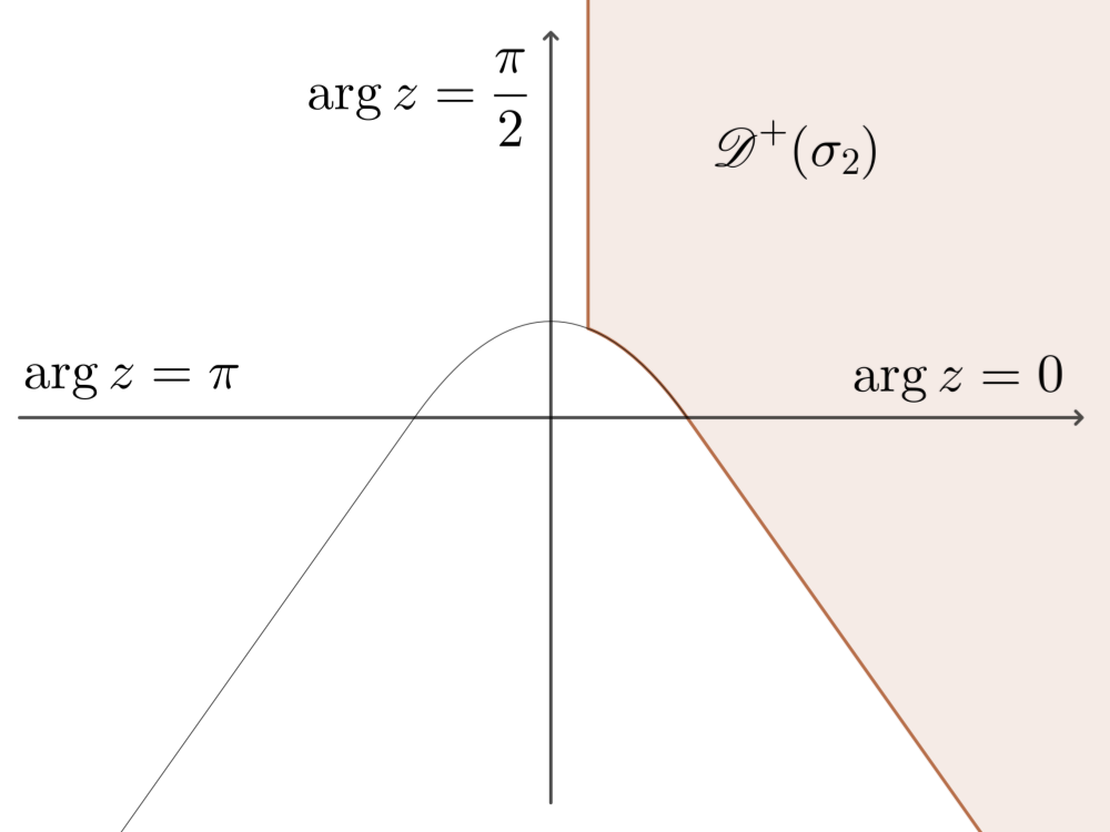
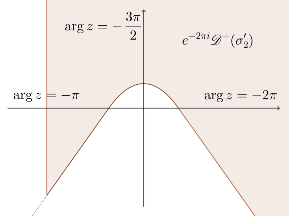
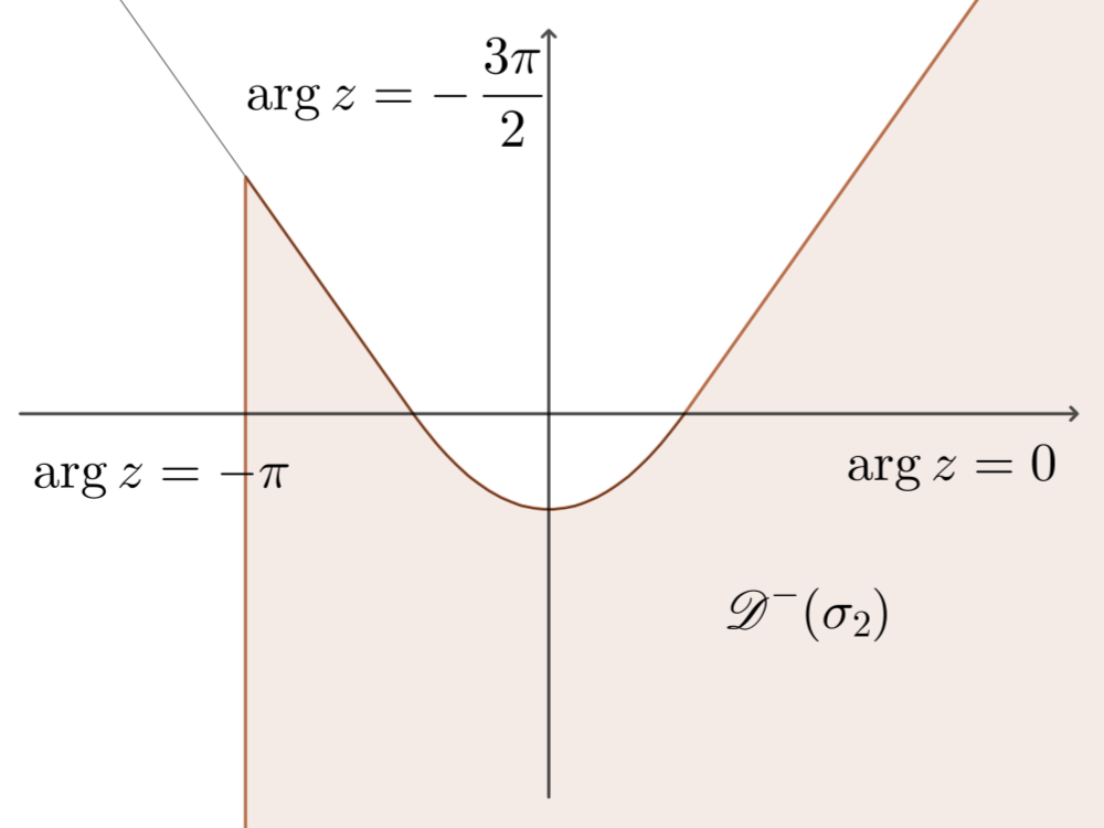
Figure 8: Top: Domains of analyticity near $\arg z=0$ with arbitrary $\sigma_{2}$ and $\sigma_{2}^{\prime}$. Bottom: Domains of analyticity near $\arg z=-\pi$ for $|\sigma_{2}|$ and  $|\sigma_{2}^{\prime}|$ small enough so as to yield non-empty intersection with $e^{-i\pi}\mathbb{R}_{>0}$.

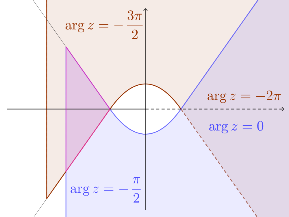
Figure 9: Left: Overlap of $\mathscr{D}^{+}(\sigma_{2})$ and $\mathscr{D}^{-}(\sigma_{2}-i)$. Right: The overlap of $\mathscr{D}^{-}(\sigma_{2})$ and $e^{-2\pi i}\mathscr{D}^{+}(\frac{\sigma_{2}}{1-i\sigma_{2}})$ is only the bounded domain on the left.

Proof.

Since $\mathscr{D}_{I^{+}}$ contains the half-plane $\{\mathop{\Re e}\nolimits(ze^{-i\theta})>\alpha(\theta)\}$ for any $\theta\in I^{+}$, it contains all the half-lines $(\frac{\alpha(\theta)}{\cos\theta},+\infty)\subset e^{i0}\mathbb{R}_{>0}$, $\theta\in\big{(}-\frac{\pi}{2},\frac{\pi}{2}\big{)}\cap I^{+}$, and thus their union $(\alpha_{0},+\infty)$. Similarly $\mathscr{D}_{I^{-}}$ contains the half-line $(\alpha_{0},+\infty)$. This implies the statement about $\mathscr{D}^{+}(\sigma_{2})\cap\mathscr{D}^{-}(\sigma_{2}^{\prime})$.

The connection formula is obtained by applying the theory of Section 2.9 to $\widetilde{G}$, viewing it as a simple $2\mathbb{Z}$-resurgent transseries and using $\omega_{1}=2$ as generator of $\Omega=2\mathbb{Z}$. Indeed, set

$$\theta^{*}\coloneqq 0,\quad I_{R}\coloneqq(-\tfrac{\pi}{2},0)\subset I^{+},\quad I_{L}\coloneqq(0,\tfrac{\pi}{2})\subset I^{-}.$$ (3.67)

Then, in view of (3.37), (2.82) with $m_{*}=1$ shows that $G^{+}(z,\sigma_{1},\sigma_{2})$ cannot differ from $G^{-}(z,\sigma_{1},\sigma_{2}-i)$ by more than $O(e^{-2\mu\mathop{\Re e}\nolimits z})$, for any $\mu\in(1,2)$, and Proposition 3.14 thus yields the conclusion. ∎

To obtain Theorem B(iii), we now use the two-parameter family of solutions

$$z\in e^{-2\pi i}\mathscr{D}^{+}(\sigma_{2})\mapsto G^{+}(e^{2\pi i}z,\sigma_{1},\sigma_{2})=\mathscr{S}^{2\pi+I^{+}}\widetilde{G}(z,\sigma_{1},\sigma_{2})$$ (3.68)

(cf. footnote 4).

Proposition 3.16 (Connection formula around the direction $\arg z=-\pi$).

Let

$$\alpha_{\pi}\coloneqq\inf\bigg{\{}\frac{\alpha(\theta)}{|\cos\theta|}\mid\theta\in\big{(}\!-\pi,-\tfrac{\pi}{2}\big{)}\bigg{\}}=\inf\bigg{\{}\frac{\alpha(\theta)}{|\cos\theta|}\mid\theta\in\big{(}\tfrac{\pi}{2},\pi\big{)}\bigg{\}}.$$ (3.69)

Then, for any $\sigma_{2},\sigma_{2}^{\prime}\in\mathbb{C}$ such that $s\coloneqq\max\big{\{}|\sigma_{2}|,|\sigma_{2}^{\prime}|\big{\}}<\frac{1}{2}e^{-2\alpha_{\pi}}$, the intersection $\mathscr{D}^{-}(\sigma_{2}^{\prime})\cap(e^{-2\pi i}\mathscr{D}^{+}(\sigma_{2}))$ contains the non-trivial line-segment $e^{-i\pi}\big{(}\alpha_{\pi},x(s)\big{)}\subset e^{-i\pi}\mathbb{R}_{>0}$, where $x(s)\coloneqq\tfrac{1}{2}\ln\tfrac{1}{2s}$.

Moreover, for any $\sigma_{1}\in\mathbb{C}$, if both $|\sigma_{2}|$ and $\left|\frac{\sigma_{2}}{1-i\sigma_{2}}\right|<\frac{1}{2}e^{-2\alpha_{\pi}}$, then

$$G^{-}(z,\sigma_{1},\sigma_{2})=G^{+}\Big{(}e^{2\pi i}z,\sigma_{1}+\log(1-i\sigma_{2}),\frac{\sigma_{2}}{1-i\sigma_{2}}\Big{)}$$ (3.70)

in the non-empty domain $z\in\mathscr{D}^{-}(\sigma_{2})\cap(e^{-2\pi i}\mathscr{D}^{+}(\frac{\sigma_{2}}{1-i\sigma_{2}}))$ (see bottom of Figure 8 and right of Figure 9).

Proof.

One can check that $\mathscr{D}_{I^{+}}$ contains all the half-lines $e^{i\pi}(\frac{\alpha(\theta)}{|\cos\theta|},+\infty)\subset e^{i\pi}\mathbb{R}_{>0}$, $\theta\in\big{(}-\pi,-\frac{\pi}{2})$, and thus their union $e^{i\pi}(\alpha_{\pi},+\infty)$. Similarly $\mathscr{D}_{I^{-}}$ contains the half-line ${\color[rgb]{.5,0,.5}e^{-i\pi}(\alpha_{\pi},+\infty)}$. Therefore

$$e^{-i\pi}(\alpha_{\pi},+\infty)\subset\mathscr{D}_{I^{-}}\cap(e^{-2\pi i}\mathscr{D}_{I^{+}}).$$ (3.71)

This implies the statement about $\mathscr{D}^{-}(\sigma_{2}^{\prime})\cap(e^{-2\pi i}\mathscr{D}^{+}(\sigma_{2}))$.

We now apply (2.82) to $\widetilde{G}_{k}$ ($k\geqslant 0$) with $\omega_{1}=-2$ and

$$\theta^{*}\coloneqq\pi,\quad I_{R}\coloneqq(\tfrac{\pi}{2},\pi)\subset I^{-},\quad I_{L}\coloneqq(\pi,\tfrac{3\pi}{2})\subset 2\pi+I^{+}.$$ (3.72)

Extending $\alpha$ by $2\pi$-periodicity, we thus take $z$ in the domain $\mathscr{D}(I_{R},\alpha)\cap\mathscr{D}(I_{L},\alpha)\subset\mathscr{D}_{I^{-}}\cap(e^{-2\pi i}\mathscr{D}_{I^{+}})$. Note that, by footnote 4, we have

$$\mathscr{S}^{I_{L}}\widetilde{G}_{k}(z)=\mathscr{S}^{2\pi+I^{+}}\widetilde{G}_{k}(z)=\mathscr{S}^{I^{+}}\widetilde{G}_{k}(e^{2\pi i}z).$$ (3.73)

In view of (3.49) there are only finitely many values of $n$ for which $\Delta_{-2n}^{+}$ does not annihilate $\widetilde{G}_{k}$, we thus get an exact formula

$$\mathscr{S}^{I^{-}}\widetilde{G}_{k}(z)=\mathscr{S}^{I_{R}}\widetilde{G}_{k}(z) =\mathscr{S}^{I_{L}}\widetilde{G}_{k}(z)+\sum_{1\leqslant n\leqslant k}e^{2nz}\mathscr{S}^{I_{L}}\Delta_{-2n}\widetilde{G}_{k}(z)$$ (3.74)

$$=\mathscr{S}^{I^{+}}\widetilde{G}_{k}(e^{2\pi i}z)+\sum_{1\leqslant n\leqslant k}e^{2nz}\mathscr{S}^{I^{+}}\Delta_{-2n}\widetilde{G}_{k}(e^{2\pi i}z).$$

Multiplying this by $\sigma_{2}^{k}$, we can take the sum over all $k\geqslant 0$ and get a convergent series if $|\sigma_{2}|$ is small enough: we just need both $\tfrac{1}{2}\ln|2\sigma_{2}|$ and $\tfrac{1}{2}\ln\big{|}\tfrac{2\sigma_{2}}{1-i\sigma_{2}}\big{|}<\mathop{\Re e}\nolimits z$, which ensures

$$z\in\mathscr{D}^{-}(\sigma_{2})\cap(e^{-2\pi i}\mathscr{D}^{+}\big{(}\tfrac{\sigma_{2}}{1-i\sigma_{2}}\big{)})$$ (3.75)

and, by virtue of (3.49)–(3.50), after adding $\sigma_{1}$ the result is (3.70). ∎

Inverting the map $(\sigma_{1},\sigma_{2})\mapsto\big{(}\sigma_{1}+\log(1-i\sigma_{2}),\frac{\sigma_{2}}{1-i\sigma_{2}}\big{)}$, we find that (3.70) is equivalent to

$$G^{+}(e^{2\pi i}z,\sigma_{1},\sigma_{2})=G^{-}(z,\sigma_{1}+\log(1+i\sigma_{2}),\frac{\sigma_{2}}{1+i\sigma_{2}}\Big{)}$$ (3.76)

in the non-empty domain $z\in\mathscr{D}^{-}(\frac{\sigma_{2}}{1+i\sigma_{2}})\cap(e^{-2\pi i}\mathscr{D}^{+}(\sigma_{2}))$ if both $|\sigma_{2}|$ and $\left|\frac{\sigma_{2}}{1+i\sigma_{2}}\right|<\frac{1}{2}e^{-2\alpha_{\pi}}$, which gives rise to the connection formula of Theorem B(iii).

3.7 Real analytic solutions and rationality of coefficients

A natural question is: For which values of $\sigma_{1}$ and $\sigma_{2}$ are the Borel sums $G^{\pm}(z,\sigma_{1},\sigma_{2})$ real analytic? This plays a crucial role in perturbation theory, as emphasized and analyzed in [5].

The answer will be obtained as a consequence of the connection formulas of the previous section. We will find for which $(\sigma_{1},\sigma_{2})$ the function $G^{-}(z,\sigma_{1},\sigma_{2})$ is real for $z$ real, i.e., since we must take $z\in\mathscr{D}^{-}(\sigma_{2})$, for $\arg z=0$ or $\arg z=-\pi$.

We first observe that, as noticed in [3], the coefficients of $\mathcal{F}^{\hskip 0.52498pt\mathrm{s}}(\lambda_{s})=\widetilde{g}(z)$ are real and rational. More generally,

Lemma 3.17.

For each $k\geqslant 0$, $\widetilde{G}_{k}(z)\in\mathbb{Q}[[z^{-1}]]$.

Proof.

The coefficients $c_{n}$ in (2.37) belong to $\mathbb{Q}$, thus the series $\widetilde{\varphi}(z)$ and $\widetilde{\psi}(z)$ of Section 2.5 belong to $\mathbb{Q}[[z^{-1}]]$. The same is true for $\widetilde{g}=\widetilde{G}_{0}$ and $\widetilde{f}$ by (3.4)–(3.5), and thus for all $\widetilde{G}_{k}$, $k\geqslant 1$, by (3.22). ∎

Now, if a summable formal series $\widetilde{a}(z)=\sum_{n\geqslant 0}a_{n}z^{-n}\in\mathbb{C}\oplus\widetilde{\mathscr{N}}(J,\beta)$ has real coefficients, that does not imply that $\mathscr{S}^{J}\widetilde{a}(z)$ is real whenever $z$ is real. What is always true is that the Borel transform $\widehat{a}(\zeta)=\sum_{n\geqslant 1}a_{n}\frac{\zeta^{n-1}}{(n-1)!}\in\mathbb{R}\{\zeta\}$ is real analytic: $\widehat{a}(\zeta)=\overline{\widehat{a}(\overline{\zeta})}$, hence the conjugate of $\mathscr{S}^{J}\widetilde{a}(\overline{z})=a_{0}+\int_{0}^{+\infty}e^{-\overline{z}\,e^{i\theta}t}\,\widehat{a}(e^{i\theta}t)e^{i\theta}dt$ (with appropriate $\theta\in J$) is seen to be

$$\overline{\mathscr{S}^{J}\widetilde{a}(\overline{z})}=\mathscr{S}^{-J}\widetilde{a}(z).$$ (3.77)

In the case of the Borel sums of the formal integral $\widetilde{G}$, since $I^{-}=-I^{+}$ and $\alpha\colon\thinspace I^{-}\cup I^{+}\to\mathbb{R}_{\geqslant 0}$ is even, we obtain $z\in\mathscr{D}^{-}(\sigma_{2})\;\Longleftrightarrow\;\overline{z}\in\mathscr{D}^{+}(\overline{\sigma}_{2})$ and, when these equivalent conditions are fulfilled,

$$\overline{G^{-}(z,\sigma_{1},\sigma_{2})}=G^{+}(\overline{z},\overline{\sigma_{1}},\overline{\sigma_{2}}).$$ (3.78)

Proof of Theorem C(i).

We first focus on the case $\arg z=0$ and write $z=re^{i0}$ with $r>0$. The proof of Proposition 3.15 shows that $\mathscr{D}_{I^{-}}\cap\mathscr{D}_{I^{+}}$ contains $(\alpha_{0},+\infty)\subset e^{i0}\mathbb{R}_{>0}$ and (3.78) shows that, for any $(\sigma_{1},\sigma_{2})\in\mathbb{C}^{2}$, the function $r\in\mathscr{D}^{-}(\sigma_{2})\cap e^{i0}\mathbb{R}_{>0}\mapsto G^{-}(r,\sigma_{1},\sigma_{2})$ is real-valued if and only if

$$G^{-}(r,\sigma_{1},\sigma_{2})=G^{+}(r,\overline{\sigma_{1}},\overline{\sigma_{2}})\quad\text{for}\enspace r>\max\{\alpha_{0},\tfrac{1}{2}\ln|2\sigma_{2}|\}.$$ (3.79)

The right-hand side of (3.79) is $G^{-}(r,\overline{\sigma_{1}},\overline{\sigma_{2}}-i)$ by (3.66), thus this is equivalent to

$$\sigma_{1}=\overline{\sigma_{1}},\quad\sigma_{2}=\overline{\sigma_{2}}-i,$$ (3.80)

which amounts to $(\sigma_{1},\sigma_{2})=(a,b-\frac{i}{2})$ where $a,b\in\mathbb{R}$.

Since $\ln|2(b-\frac{i}{2})|=\frac{1}{2}\ln(1+4b^{2})$, we see that the function $G^{-}(z,a,b-\frac{i}{2})$ is analytic in $\{\,z\in\mathscr{D}_{I^{-}}\mid\mathop{\Re e}\nolimits z>\frac{1}{4}\ln(1+4b^{2})\,\}$; it coincides with $G^{+}(z,a,b+\frac{i}{2})$ and is thus also analytic in $\{\,z\in\mathscr{D}_{I^{+}}\mid\mathop{\Re e}\nolimits z>\frac{1}{4}\ln(1+4b^{2})\,\}$.

Remark 3.18.

This is an instance of median summation. Indeed, as discussed earlier, the formal integral $\widetilde{G}(z,\sigma_{1},\sigma_{2})$ belongs to an algebra of simple $2\mathbb{Z}$-resurgent transseries on which $\mathscr{S}^{I^{+}}=\mathscr{S}^{I^{-}}\circ{{\Delta}}\hskip-6.00006pt\raisebox{1.59302pt}{\leavevmode\resizebox{2.58334pt}{}{$\mathrm{/}$}}\hskip 3.99994pt{}_{\mathbb{R}_{\geqslant 0}}^{+}$ in restriction to $z\in e^{i0}\mathbb{R}_{>0}$. In that context, we can introduce the median summation operator relative to the direction $\theta=0$:

$$\mathscr{S}_{\operatorname{med}}^{0}\coloneqq\mathscr{S}^{I^{-}}\circ({{\Delta}}\hskip-6.00006pt\raisebox{1.59302pt}{\leavevmode\resizebox{2.58334pt}{}{$\mathrm{/}$}}\hskip 3.99994pt{}_{\mathbb{R}_{\geqslant 0}}^{+})^{1/2}=\mathscr{S}^{I^{+}}\circ({{\Delta}}\hskip-6.00006pt\raisebox{1.59302pt}{\leavevmode\resizebox{2.58334pt}{}{$\mathrm{/}$}}\hskip 3.99994pt{}_{\mathbb{R}_{\geqslant 0}}^{+})^{-1/2}.$$ (3.81)

Then, (3.19) shows that the above real analytic solutions are nothing but

$$\mathscr{S}_{\operatorname{med}}^{0}\widetilde{G}(z,a,b)=G^{-}(z,a,b-\tfrac{i}{2})=G^{+}(z,a,b+\tfrac{i}{2}).$$ (3.82)

For $a,b\in\mathbb{R}$, $\widetilde{G}(z,a,b)$ is a real transseries solution to (3.2), and $\mathscr{S}_{\operatorname{med}}^{0}$ belongs to a family of summation operators that preserve realness as well as the fact of being solution to a nonlinear ODE.

Proof of Theorem C(ii).

We now consider the case $\arg z=-\pi$ and write $z=re^{-i\pi}$ with $r>0$. The proof of Proposition 3.16 shows that $\mathscr{D}_{I^{-}}\cap(e^{-2\pi i}\mathscr{D}_{I^{+}})$ contains $e^{-i\pi}(\alpha_{\pi},+\infty)$. For any $(\sigma_{1},\sigma_{2})\in\mathbb{C}^{2}$ with $|\sigma_{2}|<\tfrac{1}{2}e^{-2\alpha_{\pi}}$ (so that $\tfrac{1}{2}\ln\tfrac{1}{|2\sigma_{2}|}>\alpha_{\pi}$), the restriction of $G^{-}(\cdot\,,\sigma_{1},\sigma_{2})$ to $\mathscr{D}^{-}(\sigma_{2})\cap e^{-i\pi}\mathbb{R}_{>0}$ gives rise to the function

$$r\in(\alpha_{\pi},\tfrac{1}{2}\ln\tfrac{1}{|2\sigma_{2}|})\mapsto G^{-}(re^{-i\pi},\sigma_{1},\sigma_{2}).$$ (3.83)

In view of (3.78), this function is real-valued if and only if

$$G^{-}(re^{-i\pi},\sigma_{1},\sigma_{2})=G^{+}(re^{i\pi},\overline{\sigma_{1}},\overline{\sigma_{2}})\quad\text{for}\enspace r\in(\alpha_{\pi},\tfrac{1}{2}\ln\tfrac{1}{|2\sigma_{2}|}).$$ (3.84)

It follows from (3.76) that, for $|\sigma_{2}|$ small enough, the right-hand side of (3.84) is $G^{-}(re^{-i\pi},\overline{\sigma_{1}}+\log(1+i\overline{\sigma_{2}}),\frac{\overline{\sigma_{2}}}{1+i\,\overline{\sigma_{2}}})$, thus realness is equivalent to

$$\sigma_{1}=\overline{\sigma_{1}}+\log(1+i\overline{\sigma_{2}}),\quad\sigma_{2}=\frac{\overline{\sigma_{2}}}{1+i\,\overline{\sigma_{2}}},\quad\text{with}\enspace|\sigma_{2}|=\left|\frac{\overline{\sigma_{2}}}{1+i\,\overline{\sigma_{2}}}\right|<\tfrac{1}{2}e^{-2\alpha_{\pi}}.$$ (3.85)

The second equation in (3.85) is equivalent to $|\sigma_{2}+i|^{2}=1$, so we write $\sigma_{2}=-i(1-e^{i\theta})$ with $\theta\in\mathbb{R}$. Since $|1+i\,\overline{\sigma_{2}}|=1$, the third condition in (3.85) is equivalent to $|\sigma_{2}|^{2}<\frac{1}{4}e^{-4\alpha_{\pi}}$, or $\cos\theta>1-\frac{1}{8}e^{-4\alpha_{\pi}}$, we thus parametrize $\sigma_{2}$ by

$$\sigma_{2}=-i(1-e^{i\theta})\quad\text{with}\enspace\theta\in(-\theta_{*},\theta_{*}),\quad\text{where}\enspace\theta_{*}\coloneqq\arccos(1-\tfrac{1}{8}e^{-4\alpha_{\pi}}).$$ (3.86)

The first equation in (3.85) is then equivalent to $-2i\mathop{\Im m}\nolimits\sigma_{1}=-\log(1+i\,\overline{\sigma_{2}})=i\theta$, we thus must parametrize $\sigma_{1}$ as

$$\sigma_{1}=a-i\,\frac{\theta}{2}\quad\text{with}\enspace a\in\mathbb{R}.$$ (3.87)

We see that, with these values of $\sigma_{1}$ and $\sigma_{2}$, the function $G^{-}(z,\sigma_{1},\sigma_{2})$ is analytic in $\{\,z\in\mathscr{D}_{I^{-}}\mid\mathop{\Re e}\nolimits z>\frac{1}{2}\ln(2|1-e^{i\theta}|)\,\}$; it coincides with $G^{+}(e^{2i\pi}z,\overline{\sigma_{1}},\overline{\sigma_{2}})$ and is thus also analytic in $\{\,z\in e^{-2\pi i}\mathscr{D}_{I^{+}}\mid\mathop{\Re e}\nolimits z>\frac{1}{2}\ln(2|1-e^{i\theta}|)\,\}$, and real-valued for $\arg z=-\pi$.

Remark 3.19.

Since rational coefficients are often linked with the enumeration of geometric objects, it would be interesting to spell out the enumerative meaning of the coefficients of each $\widetilde{G}_{k}$ or of all of $\widetilde{G}$ from the geometrical and non-perturbative topological string perspective. Even more interesting would be the understanding of the enumerative nature of the connection formula between $G^{+}$ and $G^{-}$.

4 Transseries completion for the free energy in the large radius limit

In this section we will go from the resurgent properties that we have proved for the formal series obtained via Alim-Yau-Zhou’s double scaling limit ([3]) to those for the free energy as obtained via Couso-Santamaría’s large radius limit, thus rigorously proving several statements conjectured in [9]. Before doing that, we have a remark on the double scaling process.

4.1 A remark on the interpretation of Alim-Yau-Zhou’s parameter $\varepsilon$

To capture the terms $a_{g}C_{zzz}^{2g-2}(S^{zz})^{3g-3}$ of the coefficients of the total free energy $\mathcal{F}$ in (1.2), Alim-Yau-Zhou’s paper [3] employs the following double scaling:

$$g_{s}\mapsto\varepsilon^{-1}g_{s},\qquad S^{zz}\mapsto\varepsilon^{\frac{2}{3}}S^{zz},$$ (4.1)

along with $\lambda_{s}^{2}=g_{s}^{2}C_{zzz}^{2}(S^{zz})^{3}$ and $\varepsilon\to 0$ (cf. (1.4)). The indeterminate $\lambda_{s}$ in the resulting free energy $\mathcal{F}^{\hskip 0.52498pt\mathrm{s}}(\lambda_{s})$ of (1.3) is thus essentially $g_{s}C_{zzz}(S^{zz})^{3/2}$ and the small parameter $\varepsilon$ is a device used to capture the terms that are dominant when the nonholomorphic propagator $S^{zz}$ is large. In Couso-Santamaría’s large radius limit process ([9]), according to (1.7) only one variable is rescaled:

$$S^{zz}=z^{2}\Sigma,$$ (4.2)

and then one takes the limit $z\to 0$, i.e. in the $z$-space one goes to the large radius point, where the Yukawa coupling $C_{zzz}$ is singular.

The comparison between (4.1) and (4.2) prompted the author of [9] to propose the relation $\varepsilon=z^{-3}$, however this is quite misleading: on the one hand it yields a contradiction since $\varepsilon$ and $z$ could not go simultaneously to $0$, on the other hand the large radius limit $z\to 0$ is only half of the process to get the $a_{g}$’s, one must still set $g_{s}=C_{zzz}^{-1}\,\Sigma^{-3/2}\lambda_{s}$ and send $\Sigma$ to $\infty$. A better explanation is that Alim-Yau-Zhou’s double scaling limit can be slightly generalized to

$$g_{s}=\varepsilon\,C_{zzz}^{\alpha-1}\,\Sigma^{-3/2}\lambda_{s},\qquad S^{zz}=\varepsilon^{-\frac{2}{3}}\,C_{zzz}^{-2\alpha/3}\,\Sigma$$ (4.3)

with arbitrary $\alpha$ (instead of just taking $\alpha=0$), which leads to

$$\varepsilon=z^{-3}C_{zzz}^{-\alpha}.$$ (4.4)

In view of the “large radius” feature $C_{zzz}\underset{z\to 0}{\sim}\kappa z^{-3}$ used by Couso-Santamaría, this new relation results in

$$\varepsilon\underset{z\to 0}{\sim}\kappa^{-\alpha}z^{3(\alpha-1)},$$ (4.5)

which is meaningful for any $\alpha>1$.

4.2 From the double scaling limit to the large radius limit

In Section 3, we have discussed the resurgent properties of the total free energy $\mathcal{F}^{\hskip 0.52498pt\mathrm{s}}(\lambda_{s})$ of (1.3) and its transseries completion

$$\mathcal{G}(\lambda_{s},\sigma_{1},\sigma_{2})=\widetilde{G}\big{(}\tfrac{1}{3\lambda_{s}^{2}},\sigma_{1},\sigma_{2}\big{)}$$

of (3.20), solutions to the nonlinear ODE deduced from HAE via Alim-Yau-Zhou’s double scaling limit ([3])

$$\theta^{2}_{\lambda_{s}}\mathcal{F}+(\theta_{\lambda_{s}}\mathcal{F})^{2}+2\left(1-\frac{2}{3\lambda_{s}^{2}}\right)\theta_{\lambda_{s}}\mathcal{F}+\frac{5}{9}=0,\qquad\theta_{\lambda_{s}}\coloneqq\lambda_{s}\frac{\partial}{\partial\lambda_{s}}.$$ (1.5)

Recall that, in Couso-Santamaría’s large radius limit process ([9]), HAE leads to the $u$-equation instead:

$$\partial_{u}H-\frac{3}{2}g_{s}^{2}u^{3}\left(\partial_{u}H+\frac{u}{3}\partial_{u}^{2}H+\frac{u}{3}(\partial_{u}H)^{2}\right)=\frac{1}{2u}+\frac{1}{u^{2}}.$$ (1.9)

Our goal is now to discuss the resurgent properties of Couso-Santamaría’s large radius limit free energy $H^{(0),\mathrm{u}}(g_{s},u)$ of (1.8) and to employ alien calculus to derive the transseries completion $H^{\mathrm{u}}(g_{s},u,\sigma)$ of (1.10) or, equivalently,

$$\mathcal{H}^{\mathrm{u}}(g_{s},u,\sigma_{1},\sigma_{2})=\sigma_{1}+H^{\mathrm{u}}(g_{s},u,\sigma_{2}),$$ (4.6)

which will be the two-parameter transseries solution to (1.9).

The key observation is that the change of variable

$$\lambda_{s}=\phi_{g_{s}}\!(u)\coloneqq\left(\frac{g_{s}^{2}u^{3}}{(1-2g_{s}^{2}u^{2})^{3/2}}\right)^{1/2}\quad\text{(for any parameter $g_{s}\in\mathbb{C}^{*}$)}$$ (4.7)

empirically discovered in [9] (see especially [9, eqn. (48)]) allows one to directly go from (1.5) to (1.9), up to adding an elementary function of $u$ and $g_{s}$.

Proposition 4.1.

For any parameter $g_{s}\in\mathbb{C}^{*}$, the change of variable and unknown

$$H(u)=\mathcal{F}\big{(}\phi_{g_{s}}\!(u)\big{)}+R(g_{s},u)$$ (4.8)

with $\phi_{g_{s}}$ as in (4.7) and

$$R(g_{s},u)\coloneqq\frac{1}{4}\log\Big{(}\frac{u^{2}}{1-2g_{s}^{2}u^{2}}\Big{)}+\frac{(1-2g_{s}^{2}u^{2})^{3/2}-1}{3g_{s}^{2}u^{3}}$$ (4.9)

makes the two nonlinear ODEs (1.5) and (1.9) equivalent.

Proof.

As observed at the beginning of Section 3, the change of variable and unknown $\mathcal{F}(\lambda_{s})=g(\frac{1}{3\lambda_{s}^{2}})$ transforms (1.5) into

$$g^{\prime\prime}+(g^{\prime})^{2}+2g^{\prime}+\frac{5}{36}z_{1}^{-2}=0,$$ (3.2)

where we now call $z_{1}=\frac{1}{3\lambda_{s}^{2}}$ (instead of $z$ as in Section 3) the variable with respect to which the unknown $g=g(z_{1})$ is expressed. Therefore, one just needs to check that the change of variable and unknown

$$z_{1}=\frac{1}{3\lambda_{s}^{2}} =\frac{1}{3\phi_{g_{s}}\!(u)^{2}}=\frac{1}{3g_{s}^{2}u^{3}}(1-2g_{s}^{2}u^{2})^{3/2},$$ (4.10)

$$H(u) =g(z_{1})+R(g_{s},u)$$ (4.11)

makes (3.2) and (1.9) equivalent. This computation is left to the reader. ∎

Proposition 4.2.

The large radius perturbative series $H^{(0),\mathrm{u}}$ defined in [9] is

$$H^{(0),\mathrm{u}}(g_{s},u)=R(g_{s},u)+\mathcal{F}^{\hskip 0.52498pt\mathrm{s}}\big{(}\phi_{g_{s}}\!(u)\big{)},$$ (4.12)

where $R(g_{s},u)$ is defined by (4.9) (or rather its Taylor expansion with respect to $g_{s}^{2}$) and the second term of the right-hand side is understood as the substitution of the convergent series

$$\lambda_{s}^{2}=\phi_{g_{s}}\!(u)^{2}=\sum_{\ell\geqslant 1}\Big{(}\frac{(2\ell-1)!}{2^{\ell-1}(\ell-1)!^{2}}u^{2\ell+1}\Big{)}g_{s}^{2\ell}$$ (4.13)

in the formal power series $\mathcal{F}^{\hskip 0.52498pt\mathrm{s}}(\lambda_{s})=\sum_{\ell\geqslant 1}a_{\ell+1}\lambda_{s}^{2\ell}$ of (1.3). Among the formal series in $g_{s}^{2}$ with $u$-dependent coefficients, the solutions to (1.9) are the formal series

$$C(g_{s})+H^{(0),\mathrm{u}}(g_{s},u)\quad\text{with arbitrary formal series}\enspace C(g_{s})\in\mathbb{C}[[g_{s}]].$$ (4.14)

From the perspective of perturbative free energy, we thus have a direct relationship

Note that, as mentioned in (1.8), the formula for $H^{(0),\mathrm{u}}$ contains a contribution of genus $g=\ell+1=1$, i.e. a constant term in $g_{s}^{2}$ (hinted at in [9]), since

$$R(g_{s},u)=-\frac{1}{u}+\frac{1}{2}\log u+H^{(0),\mathrm{u}}_{\mathrm{conv}}(g_{s},u)\quad\text{with $H^{(0),\mathrm{u}}_{\mathrm{conv}}(g_{s},u)=O(g_{s}^{2})$,}$$ (4.15)

but by convention the expansion stemming from $\mathcal{F}^{\hskip 0.52498pt\mathrm{s}}$ starts from genus $g=\ell+1=2$ (cf. (1.3)).

Proof of Proposition 4.2.

If one starts with arbitrary $\mathcal{F}(\lambda_{s})\in\mathbb{C}[[\lambda_{s}^{2}]]$, performs the substitution (4.13) and adds $R(g_{s},u)$,

then the result is a series $H(g_{s},u)$ in the indeterminate $g_{s}^{2}$ with $u$-dependent coefficients. The computation outlined in the proof of Proposition 4.1 shows that if the initial series $\mathcal{F}(\lambda_{s})$ solves (1.5), then the resulting series solves (1.9). In particular, the right-hand side of (4.12) is a formal solution to (1.9).

On the other hand, when plugging an arbitrary formal series with $u$-dependent coefficients $H=\sum_{k\geqslant 0}H_{k}(u)g_{s}^{2k}$ into (1.9), it is easy to see that each term $H_{k}$ is determined by the previous ones up to the addition of an arbitrary complex constant, thus

$$H=C(g_{s})+R(g_{s},u)+\mathcal{F}^{\hskip 0.52498pt\mathrm{s}}\big{(}\phi_{g_{s}}\!(u)\big{)}\enspace\text{with arbitrary}\enspace C(g_{s})\in\mathbb{C}[[g_{s}]].$$ (4.16)

To conclude the proof, we just need to check that among these solutions, $H^{(0),\mathrm{u}}(g_{s},u)$ is the one corresponding to the choice $C(g_{s})\equiv 0$. To that end, we observe that $R(g_{s},u)+\mathcal{F}^{\hskip 0.52498pt\mathrm{s}}\big{(}\phi_{g_{s}}\!(u)\big{)}$ is a formal series in $g_{s}^{2}$ all of whose coefficients are polynomials in $u$ that vanish at $u=0$, with the only exception of the constant term in $g_{s}^{2}$ that stems from (4.15). But [9, eqn. (47)] shows that the coefficient of $g_{s}^{2(g-1)}$ in $H^{(0),\mathrm{u}}(g_{s},u)$ must vanish when $u=0$ for each $g\geqslant 2$; this requirement shows that $C(g_{s})\equiv 0$ is the only possibility (note that the constant term with respect to $g_{s}$ in $H^{(0),\mathrm{u}}(g_{s},u)$, corresponding to $g=1$, is a function of $u$ that is only determined up to an additive constant and our choice is only a matter of convention). ∎

4.3 Resurgent structure of the transseries completion

We know from Section 3 that $\mathcal{F}^{\hskip 0.52498pt\mathrm{s}}(\lambda_{s})$ is resurgent in $z_{1}=\frac{1}{3\lambda_{s}^{2}}=\frac{1}{3\phi_{g_{s}}\!(u)^{2}}$. Now, the core of the above relation (4.12) can be viewed as a tangent-to-identity change of variable with respect to the variable $z_{2}=\frac{1}{3g_{s}^{2}u^{3}}$, in the sense that (4.10) can be rephrased as

$$z_{1}=z_{2}\Big{(}1-\frac{2}{3u}z_{2}^{-1}\Big{)}^{3/2}=z_{2}+\varphi_{u}(z_{2}),\qquad\varphi_{u}(z_{2})\in\mathbb{C}\{z_{2}^{-1}\},$$ (4.17)

where $u\in\mathbb{C}^{*}$ is now treated as a parameter. We can thus obtain the resurgence in $z_{2}$ of $H^{(0),\mathrm{u}}(g_{s},u)$ from general resurgence theory, and alien calculus then produces a transseries completion that formally solves the $u$-equation (1.9):

Theorem A’.

(i) The large radius limit free energy $H^{(0),\mathrm{u}}(g_{s},u)$ in (1.8) with $u\in\mathbb{C}^{\ast}$ treated as parameter is a divergent simple $2\mathbb{Z}$-resurgent series with respect to the variable $z_{2}=\frac{1}{3g^{2}_{s}u^{3}}$, and thus a divergent simple $\frac{2}{3u^{3}}\mathbb{Z}$-resurgent series in the variable $\frac{1}{g_{s}^{2}}$.

(ii) On $H^{(0),\mathrm{u}}(g_{s},u)$ viewed as a resurgent series in $z_{2}$, the actions of the algebra automorphisms $\exp(\sigma e^{-2z_{2}}\Delta_{2})$ and $({{\Delta}}\hskip-6.00006pt\raisebox{1.59302pt}{\leavevmode\resizebox{2.58334pt}{}{$\mathrm{/}$}}\hskip 3.99994pt{}_{\mathbb{R}_{\geqslant 0}}^{+})^{\sigma}=\exp(\sigma{{\Delta}}\hskip-6.00006pt\raisebox{1.59302pt}{\leavevmode\resizebox{2.58334pt}{}{$\mathrm{/}$}}\hskip 3.99994pt{}_{\mathbb{R}_{\geqslant 0}})$ of $\widetilde{\mathscr{R}}_{2\mathbb{Z}}[[\sigma,e^{-2z_{2}}]]$ coincide, and $H^{(0),\mathrm{u}}(g_{s},u)$ can be embedded in a two-parameter transseries

$$\mathcal{H}^{\mathrm{u}}(g_{s},u,\sigma_{1},\sigma_{2})=\sigma_{1}+H^{(0),\mathrm{u}}(g_{s},u)+\sum_{n\geqslant 1}\sigma_{2}^{n}e^{-\frac{2n}{3g_{s}^{2}u^{3}}}H^{(n),\mathrm{u}}(g_{s},u)$$ (4.18)

solution to (1.9) defined by

$$\mathcal{H}^{\mathrm{u}}\coloneqq\big{(}{{\Delta}}\hskip-6.00006pt\raisebox{1.59302pt}{\leavevmode\resizebox{2.58334pt}{}{$\mathrm{/}$}}\hskip 3.99994pt{}_{\mathbb{R}_{\geqslant 0}}^{+}\big{)}^{-i\sigma_{2}}\big{[}\sigma_{1}+H^{(0),\mathrm{u}}(g_{s},u)\big{]}.$$ (4.19)

The transseries $\mathcal{H}^{\mathrm{u}}$ is related to the transseries $\widetilde{G}$ defined by (3.18) by

$$\mathcal{H}^{\mathrm{u}}(g_{s},u,\sigma_{1},\sigma_{2})=\widetilde{G}\big{(}z_{2}+\varphi_{u}(z_{2}),\sigma_{1},-\sigma_{2}\big{)}+R(g_{s},u)\quad\text{with}\enspace z_{2}=\frac{1}{3g^{2}_{s}u^{3}}.$$ (4.20)

(iii) One also has, in terms of the transseries $\mathcal{G}(\lambda_{s},\sigma_{1},\sigma_{2})$ of (1.11) (formal integral of the double scaling limit HAE, as in Theorem A(ii)),

$$\mathcal{H}^{\mathrm{u}}(g_{s},u,\sigma_{1},\sigma_{2})=\mathcal{G}\big{(}\phi_{g_{s}}\!(u),\sigma_{1},-\sigma_{2})+R(g_{s},u).$$ (4.21)

(iv) For each $n\geqslant 1$, the $n$th component of the transseries (4.18) involves

$$H^{(n),\mathrm{u}}(g_{s},u)=-\frac{1}{n}e^{\frac{2n}{u}}+\sum\limits_{g=1}^{\infty}g_{s}^{2g}e^{\frac{2n}{u}}u^{g}Pol_{n}(u,2g),$$ (4.22)

which is a simple $2\mathbb{Z}$-resurgent series in $z_{2}$ where, for each $g\geqslant 1$, $Pol_{n}(u,2g)$ is a polynomial in $u$ of degree $2g$ with rational coefficients.

Remark 4.3.

(1) Here, for sake of simplicity, we stick to $2\mathbb{Z}$-resurgence in the variable $z_{2}=\frac{1}{3g^{2}_{s}u^{3}}$ for fixed $u\in\mathbb{C}^{*}$ and the operator ${{\Delta}}\hskip-6.00006pt\raisebox{1.59302pt}{\leavevmode\resizebox{2.58334pt}{}{$\mathrm{/}$}}\hskip 3.99994pt{}_{\mathbb{R}_{\geqslant 0}}^{+}=\exp\!\big{(}\sum_{k=1}^{\infty}e^{-2kz}\Delta_{2k}\big{)}$ acts on the corresponding algebra of transseries. This is trivially equivalent to $\frac{2}{3u^{3}}\mathbb{Z}$-resurgence in the variable $\frac{1}{g_{s}^{2}}$ and can be viewed as an elementary instance of duality between equational resurgence and parametric resurgence first introduced in [13].

(2) The coefficients in Theorem A’(iv) are rational, a phenomenon parallel to Lemma 3.17.

Note that we choose to use $-i\sigma_{2}$ as power in (4.19) rather than $i\sigma_{2}$ as in (3.18) (and consequently need to change $\sigma_{2}$ into $-\sigma_{2}$ when going from $\widetilde{G}$ to $\mathcal{H}^{\mathrm{u}}$ in (4.20)) just to align with the corresponding formulas in [9].

Proof of Theorem A’.

(i) For the sake of clarity we use different notation for the series according as they are expressed in the variable $g_{s}^{2}$ or in the variable $z_{2}$:

$$\widetilde{H}^{(0),\mathrm{u}}(z_{2},u)\coloneqq H^{(0),\mathrm{u}}(g_{s},u)\in\mathbb{C}[[z_{2}^{-1}]],\quad\widetilde{R}_{u}(z_{2})\coloneqq R(g_{s},u)\in\mathbb{C}\{z_{2}^{-1}\}$$ (4.23)

with $z_{2}=\frac{1}{3g^{2}_{s}u^{3}}$, where $u\in\mathbb{C}^{*}$ is treated as a fixed parameter. In view of (3.1), the first statement of Proposition 4.2 thus amounts to

$$\widetilde{H}^{(0),\mathrm{u}}(z_{2},u)=\widetilde{g}\big{(}z_{2}+\varphi_{u}(z_{2})\big{)}+\widetilde{R}_{u}(z_{2}),$$ (4.24)

where $\varphi_{u}$ stems from (4.17):

$$\varphi_{u}(z_{2})=z_{2}\big{(}(1-\tfrac{2}{3u}z_{2}^{-1})^{3/2}-1\big{)}=\sum_{n=1}^{\infty}\binom{\frac{3}{2}}{n}\Big{(}\!-\frac{2}{3u}\Big{)}^{n}z_{2}^{-(n-1)}\in\mathbb{C}\{z_{2}^{-1}\}.$$ (4.25)

In (4.24) we have $\widetilde{R}_{u},\varphi_{u}\in\mathbb{C}\{z_{2}^{-1}\}\subset\widetilde{\mathscr{R}}_{2\mathbb{Z}}^{\operatorname{simp}}$ and, according to Proposition 3.3, $\widetilde{g}\in\widetilde{\mathscr{R}}_{2\mathbb{Z}}^{\operatorname{simp}}$. We can thus apply Theorem 2.10 to $\widetilde{H}^{(0),\mathrm{u}}=\widetilde{g}\circ(id+\varphi_{u})+\widetilde{R}_{u}$: according to (2.70), $\widetilde{H}^{(0),\mathrm{u}}\in\widetilde{\mathscr{R}}_{2\mathbb{Z}}^{\operatorname{simp}}$. Moreover, $\widetilde{H}^{(0),\mathrm{u}}$ is divergent because $\widetilde{g}$ is divergent.

(ii) Theorem 2.10 also entails, according to (2.71), that

$$\Delta_{\omega}\widetilde{H}^{(0),\mathrm{u}}=e^{-\omega\varphi_{u}}\cdot(\Delta_{\omega}\widetilde{g})\circ(id+\varphi_{u})\quad\text{for every $\omega\in 2\mathbb{Z}^{*}$}$$ (4.26)

(since $\varphi_{u}$ is convergent and thus $\Delta_{\omega}\varphi_{u}=0$) and, consequently,

$$\big{(}{{\Delta}}\hskip-6.00006pt\raisebox{1.59302pt}{\leavevmode\resizebox{2.58334pt}{}{$\mathrm{/}$}}\hskip 3.99994pt{}_{\mathbb{R}_{\geqslant 0}}^{+}\big{)}^{\sigma}\widetilde{H}^{(0),\mathrm{u}}=\big{(}{{\Delta}}\hskip-6.00006pt\raisebox{1.59302pt}{\leavevmode\resizebox{2.58334pt}{}{$\mathrm{/}$}}\hskip 3.99994pt{}_{\mathbb{R}_{\geqslant 0}}^{+}\big{)}^{\sigma}\widetilde{g}\circ(id+\varphi_{u})+\widetilde{R}_{u}\quad\text{for any $\sigma\in\mathbb{C}$.}$$ (4.27)

Point (ii) of Theorem A’ thus follows from Proposition 3.4, which says that

$$\exp(i\sigma_{2}e^{-2z_{1}}\Delta_{2})(\sigma_{1}+\widetilde{g})=\big{(}{{\Delta}}\hskip-6.00006pt\raisebox{1.59302pt}{\leavevmode\resizebox{2.58334pt}{}{$\mathrm{/}$}}\hskip 3.99994pt{}_{\mathbb{R}_{\geqslant 0}}^{+}\big{)}^{i\sigma_{2}}(\sigma_{1}+\widetilde{g})=\widetilde{G}(z_{1},\sigma_{1},\sigma_{2}).$$ (4.28)

In particular, we get simple $2\mathbb{Z}$-resurgent series $\widetilde{H}^{(n),\mathrm{u}}(z_{2},u)=H^{(n),\mathrm{u}}(g_{s},u)$, $n\geqslant 1$, as components of the transseries

$$\widetilde{\mathcal{H}}^{\mathrm{u}}_{\mid(\sigma_{1},\sigma_{2})}\coloneqq\big{(}{{\Delta}}\hskip-6.00006pt\raisebox{1.59302pt}{\leavevmode\resizebox{2.58334pt}{}{$\mathrm{/}$}}\hskip 3.99994pt{}_{\mathbb{R}_{\geqslant 0}}^{+}\big{)}^{-i\sigma_{2}}\big{[}\sigma_{1}+\widetilde{H}^{(0),\mathrm{u}}\big{]}=\widetilde{G}\circ(id+\varphi_{u})_{\mid(\sigma_{1},-\sigma_{2})}+\widetilde{R}_{u}$$ (4.29)

(where the notation $K_{\mid(\sigma_{1},\pm\sigma_{2})}$ indicates that the arguments $(\sigma_{1},\sigma_{2})$ of $K$ must be replaced with $(\sigma_{1},\pm\sigma_{2})$). Since neither $\varphi_{u}$ nor $\widetilde{R}_{u}$ depend on the transseries parameter $\sigma_{2}$ (only $\widetilde{G}$ does), the coefficient of $\sigma_{2}^{n}$ in (4.29) is

$$e^{-2nz_{2}}\widetilde{H}^{(n),\mathrm{u}}(z_{2},u)=(-1)^{n}e^{-2n(z_{2}+\varphi_{u}(z_{2}))}\widetilde{G}_{n}\big{(}z_{2}+\varphi_{u}(z_{2})\big{)}\quad\text{for each $n\geqslant 1$,}$$ (4.30)

where the components $\widetilde{G}_{n}$ of $\widetilde{G}$ are the simple $2\mathbb{Z}$-resurgent series of Proposition 3.4.

(iii) We now return to the variable $g_{s}^{2}$ and focus on the coefficients of the expansion of $H^{(n),\mathrm{u}}$ in powers of this indeterminate:

$$H^{(n),\mathrm{u}}(g_{s},u)=\sum_{g\geqslant 0}H^{(n),\mathrm{u}}_{g}(u)\,g_{s}^{2g}.$$ (4.31)

We first rephrase (4.29) by using the transseries $\mathcal{G}$ of (1.11) and (3.20)

$$\mathcal{G}(\lambda_{s},\sigma_{1},\sigma_{2})=\widetilde{G}(z_{1}=\tfrac{1}{3\lambda_{s}^{2}},\sigma_{1},\sigma_{2})=\sigma_{1}+\sum_{n\geqslant 0}\sigma_{2}^{n}\,e^{-\frac{2n}{3\lambda_{s}^{2}}}\,\mathcal{G}_{n}(\lambda_{s})$$

where, according to Lemma 3.17 and (3.22),

$$\mathcal{G}_{n}(\lambda_{s})=\sum_{k\geqslant 0}\mathcal{G}_{n,k}\lambda_{s}^{2k}\in\mathbb{Q}[[\lambda_{s}^{2}]]\quad\text{with}\enspace\mathcal{G}_{n,0}=\frac{(-1)^{n-1}}{n}.$$ (4.32)

When returning to the indeterminate $g_{s}^{2}$, we must replace the change of variable $z_{2}=(id+\varphi_{u})(z_{1})$ by the change of variable $\lambda_{s}^{2}=\phi_{g_{s}}\!(u)^{2}$ and (4.29) thus becomes (4.21).

(iv) We just obtained

$$\mathcal{H}^{\mathrm{u}}(g_{s},u,\sigma_{1},\sigma_{2})=\sigma_{1}+\sum_{n\geqslant 0}(-\sigma_{2})^{n}e^{-\frac{2n}{3\phi_{g_{s}}\!(u)^{2}}}\mathcal{G}_{n}\big{(}\phi_{g_{s}}\!(u)\big{)}+R(g_{s},u).$$ (4.33)

When extracting the coefficient of $\sigma_{2}^{n}$ for any $n\geqslant 1$ in this relation, we must take care of the discrepancy between $e^{-\frac{2n}{3\phi_{g_{s}}\!(u)^{2}}}$ and $e^{-\frac{2n}{3g_{s}^{2}u^{3}}}$. Since

$$\frac{1}{3\phi_{g_{s}}\!(u)^{2}} -\frac{1}{3g_{s}^{2}u^{3}}=-\frac{1}{u}+g_{s}^{2}u\,c_{-}\!(g_{s}^{2}u^{2}) c_{-}\!(t)\in\mathbb{Q}[[t]],$$ with

$$\phi_{g_{s}}\!(u)^{2} =g_{s}^{2}u^{3}\big{(}1+g_{s}^{2}u^{2}c_{+}\!(g_{s}^{2}u^{2})\big{)} c_{+}\!(t)\in\mathbb{Q}[[t]],$$ with

we get

$$H^{(n),\mathrm{u}} =(-1)^{n}\,e^{-2n(-\frac{1}{u}+g_{s}^{2}u\,c_{-}\!)}\,\mathcal{G}_{n}\big{(}\phi_{g_{s}}\!(u)^{2}\big{)}$$

$$=e^{\frac{2n}{u}}\Big{(}\sum_{\ell\geqslant 0}\frac{(-2n)^{\ell}}{\ell!}g_{s}^{2\ell}u^{\ell}c_{-}^{\ell}\Big{)}\Big{(}\sum_{k\geqslant 0}(-1)^{n}\mathcal{G}_{n,k}\,g_{s}^{2k}u^{3k}(1+g_{s}^{2}u^{2}c_{+}\!)^{k}\Big{)}$$

$$=e^{\frac{2n}{u}}\Big{(}-\frac{1}{n}+\sum_{g\geqslant 1}g_{s}^{2g}\sum_{\ell+k+r=g}\frac{(-2n)^{\ell}}{\ell!}(-1)^{n}\mathcal{G}_{n,k}\,c_{\ell,k,r}\,u^{\ell+2r+3k}\Big{)},$$

where the rational coefficients $c_{\ell,k,r}$ are defined by the generating series

$$c_{-}\!(t)^{\ell}\big{(}1+tc_{+}\!(t)\big{)}^{k}=\sum_{r\geqslant 0}c_{\ell,k,r}t^{r}.$$ (4.34)

This matches the description of $H^{(n),\mathrm{u}}$ announced in (4.22). ∎

Remark 4.4.

We recover the same family of polynomials with rational coefficients as in Couso-Santamaría’s article. For instance, for the first two nontrivial poynomials associated with $n=1$, our computations give

$$Pol_{1}(u,2)=\frac{5u^{2}}{12}+1,\quad Pol_{1}(u,4)=-\frac{25u^{4}}{288}+\frac{5u^{3}}{4}-\frac{5u^{2}}{12}+\frac{u}{3}-\frac{1}{2},$$ (4.35)

in acccordance with [9, eqns. (55)-(56)].

We now establish the Bridge Equation and compute the Stokes phenomena for $\mathcal{H}^{\mathrm{u}}(g_{s},u,\sigma_{1},\sigma_{2})$, our transseries solution to (1.9).

Theorem A”.

(i) With respect to the resurgence variable $z_{2}=\frac{1}{3g_{s}^{2}u^{3}}$, we have $\Delta_{\omega}\mathcal{H}^{\mathrm{u}}=0$ for all $\omega\in 2\mathbb{Z}^{*}\setminus\{-2,2\}$, and

$$\Delta_{2}\mathcal{H}^{\mathrm{u}}(g_{s},u,\sigma_{1},\sigma_{2}) =i\,e^{2z_{2}}\frac{\partial}{\partial\sigma_{2}}\mathcal{H}^{\mathrm{u}}(g_{s},u,\sigma_{1},\sigma_{2})$$ (4.36)

$$\Delta_{-2}\mathcal{H}^{\mathrm{u}}(g_{s},u,\sigma_{1},\sigma_{2}) =i\,e^{-2z_{2}}\Big{(}\sigma_{2}\frac{\partial}{\partial\sigma_{1}}\mathcal{H}^{\mathrm{u}}(g_{s},u,\sigma_{1},\sigma_{2})-\sigma_{2}^{2}\frac{\partial}{\partial\sigma_{2}}\mathcal{H}^{\mathrm{u}}(g_{s},u,\sigma_{1},\sigma_{2})\Big{)}.$$ (4.37)

(ii) The action of the symbolic Stokes automorphism on $\mathcal{H}^{\mathrm{u}}$ is given by

$${{\Delta}}\hskip-6.00006pt\raisebox{1.59302pt}{\leavevmode\resizebox{2.58334pt}{}{$\mathrm{/}$}}\hskip 3.99994pt{}_{\mathbb{R}_{\geqslant 0}}^{+}\mathcal{H}^{\mathrm{u}}(g_{s},u,\sigma_{1},\sigma_{2}) =\mathcal{H}^{\mathrm{u}}(g_{s},u,\sigma_{1},\sigma_{2}+i),$$ (4.38)

$${{\Delta}}\hskip-6.00006pt\raisebox{1.59302pt}{\leavevmode\resizebox{2.58334pt}{}{$\mathrm{/}$}}\hskip 3.99994pt{}_{\mathbb{R}_{\leqslant 0}}^{+}\mathcal{H}^{\mathrm{u}}(g_{s},u,\sigma_{1},\sigma_{2}) =\mathcal{H}^{\mathrm{u}}(g_{s},u,\sigma_{1}+\log(1+i\sigma_{2}),\frac{\sigma_{2}}{1+i\sigma_{2}}\big{)}.$$ (4.39)

Proof.

(i) Treating $u\in\mathbb{C}^{*}$ as a parameter and switching to $\widetilde{\mathcal{H}}^{\mathrm{u}}(z_{2},u,\sigma_{1},\sigma_{2})$ explicitly viewed as a transseries in the variable $z_{2}=\frac{1}{3g_{s}^{2}u^{3}}$, we have seen in (4.29) that

$$\widetilde{\mathcal{H}}^{\mathrm{u}}_{\mid(\sigma_{1},\sigma_{2})}=\widetilde{G}_{\mid(\sigma_{1},-\sigma_{2})}\circ(id+\varphi_{u})+\widetilde{R}_{u}.$$ (4.40)

The Alien Calculus rule (2.71) thus yields

$$\Delta_{\omega}\widetilde{\mathcal{H}}^{\mathrm{u}}_{\mid(\sigma_{1},\sigma_{2})}=e^{-\omega\varphi_{u}}(\Delta_{\omega}\widetilde{G})_{\mid(\sigma_{1},-\sigma_{2})}\circ(id+\varphi_{u})+\widetilde{R}_{u}.$$ (4.41)

Plugging there the formula for $\Delta_{\omega}\widetilde{G}$ obtained in Proposition 3.6, we get $\Delta_{\omega}\widetilde{\mathcal{H}}^{\mathrm{u}}=0$ for all $\omega\in 2\mathbb{Z}^{*}\setminus\{-2,2\}$,

$$\Delta_{2}\widetilde{\mathcal{H}}^{\mathrm{u}}=-i\,e^{-2\varphi_{u}}\,e^{2(z_{2}+\varphi_{u})}\Big{(}\frac{\partial}{\partial\sigma_{2}}\widetilde{G}\Big{)}_{\mid(\sigma_{1},-\sigma_{2})}\circ(id+\varphi_{u})=i\,e^{2z_{2}}\frac{\partial}{\partial\sigma_{2}}\widetilde{\mathcal{H}}^{\mathrm{u}}$$ (4.42)

and

$$\Delta_{-2}\widetilde{\mathcal{H}}^{\mathrm{u}}=-i\,e^{2\varphi_{u}}\,e^{-2(z_{2}+\varphi_{u})}\Big{(}\sigma_{2}\frac{\partial}{\partial\sigma_{1}}\widetilde{G}-\sigma_{2}^{2}\frac{\partial}{\partial\sigma_{2}}\widetilde{G}\Big{)}_{\mid(\sigma_{1},-\sigma_{2})}\circ(id+\varphi_{u})\\[4.30554pt] =-i\,e^{-2z_{2}}\Big{(}-\sigma_{2}\frac{\partial}{\partial\sigma_{1}}\widetilde{\mathcal{H}}^{\mathrm{u}}+\sigma_{2}^{2}\frac{\partial}{\partial\sigma_{2}}\widetilde{\mathcal{H}}^{\mathrm{u}}\Big{)}.$$ (4.43)

(ii) Similarly, since $\varphi_{u}(z_{2})\in\mathbb{C}\{z_{2}^{-1}\}$, Alien Calculus yields

$${{\Delta}}\hskip-6.00006pt\raisebox{1.59302pt}{\leavevmode\resizebox{2.58334pt}{}{$\mathrm{/}$}}\hskip 3.99994pt{}_{d}^{+}\widetilde{\mathcal{H}}^{\mathrm{u}}_{\mid(\sigma_{1},\sigma_{2})}=\big{(}{{\Delta}}\hskip-6.00006pt\raisebox{1.59302pt}{\leavevmode\resizebox{2.58334pt}{}{$\mathrm{/}$}}\hskip 3.99994pt{}_{d}^{+}\widetilde{G}\big{)}_{\mid(\sigma_{1},-\sigma_{2})}\circ(id+\varphi_{u})+\widetilde{R}_{u}$$ (4.44)

for $d=\mathbb{R}_{\leqslant 0}$ or $\mathbb{R}_{\geqslant 0}$, where the latter case requires the same care as in Section 3.4.2 (see especially Lemma 3.10). In view of (3.37), we get

$${{\Delta}}\hskip-6.00006pt\raisebox{1.59302pt}{\leavevmode\resizebox{2.58334pt}{}{$\mathrm{/}$}}\hskip 3.99994pt{}_{\mathbb{R}_{\geqslant 0}}^{+}\widetilde{\mathcal{H}}^{\mathrm{u}}=\big{(}{{\Delta}}\hskip-6.00006pt\raisebox{1.59302pt}{\leavevmode\resizebox{2.58334pt}{}{$\mathrm{/}$}}\hskip 3.99994pt{}_{\mathbb{R}_{\geqslant 0}}^{+}\widetilde{G}\big{)}_{\mid(\sigma_{1},-\sigma_{2})}\circ(id+\varphi_{u})+\widetilde{R}_{u}=\widetilde{G}\big{(}z_{2}+\varphi_{u},\sigma_{1},\sigma_{2}-i\big{)}_{\mid(\sigma_{1},-\sigma_{2})}+\widetilde{R}_{u}\\[4.30554pt] =\widetilde{G}\big{(}z_{2}+\varphi_{u},\sigma_{1},-\sigma_{2}-i\big{)}+\widetilde{R}_{u}=\widetilde{\mathcal{H}}^{\mathrm{u}}(z_{2},\sigma_{1},\sigma_{2}+i),$$

while (3.48) yields

$${{\Delta}}\hskip-6.00006pt\raisebox{1.59302pt}{\leavevmode\resizebox{2.58334pt}{}{$\mathrm{/}$}}\hskip 3.99994pt{}_{\mathbb{R}_{\leqslant 0}}^{+}\widetilde{\mathcal{H}}^{\mathrm{u}}=\big{(}{{\Delta}}\hskip-6.00006pt\raisebox{1.59302pt}{\leavevmode\resizebox{2.58334pt}{}{$\mathrm{/}$}}\hskip 3.99994pt{}_{\mathbb{R}_{\leqslant 0}}^{+}\widetilde{G}\big{)}_{\mid(\sigma_{1},-\sigma_{2})}\circ(id+\varphi_{u})+\widetilde{R}_{u}\\[4.30554pt] =\widetilde{G}\big{(}z_{2}+\varphi_{u},\sigma_{1}+\log(1-i\sigma_{2}),\frac{\sigma_{2}}{1-i\sigma_{2}}\big{)}_{\mid(\sigma_{1},-\sigma_{2})}+\widetilde{R}_{u}\\[4.30554pt] =\widetilde{G}\big{(}z_{2}+\varphi_{u},\sigma_{1}+\log(1+i\sigma_{2}),-\frac{\sigma_{2}}{1+i\sigma_{2}}\big{)}+\widetilde{R}_{u}=\widetilde{\mathcal{H}}^{\mathrm{u}}(z_{2},\sigma_{1}+\log(1+i\sigma_{2}),\frac{\sigma_{2}}{1+i\sigma_{2}}).$$

∎

4.4 Summability of the large radius expansions, real analytic solutions and rationality of coefficients

We now deduce from the previous section summability results for the formal series $H^{(n),\mathrm{u}}(g_{s},u)$ with respect to $z_{2}$.

Theorem B’.

(i) For every $u\in\mathbb{C}^{*}$, the perturbative solution $H^{(0),\mathrm{u}}(g_{s},u)$ to (1.9) is $1$-summable in the directions of $(-2\pi,0)$ with respect to the variable $z_{2}=\frac{1}{3g_{s}^{2}u^{3}}$ and each $H^{(n),\mathrm{u}}(g_{s},u)$, $n\geqslant 1$, is $1$-summable with respect to $z_{2}$ in the directions of both

$$I^{+}=(-\pi,0)\enspace\text{and}\enspace I^{-}=(0,\pi).$$ (4.45)

There exist sectorial neighbourhoods of infinity $\mathscr{D}_{I^{+}}^{\prime}(u)$ and $\mathscr{D}_{I^{-}}^{\prime}(u)$ of opening $2\pi$, with $\mathscr{D}_{I^{\pm}}^{\prime}(u)$ centred on $\arg z_{2}=\pm\frac{\pi}{2}$, such that, for each choice of sign and each $(\sigma_{1},\sigma_{2})\in\mathbb{C}^{2}$, the series of functions

$$\mathcal{H}^{\mathrm{u}}_{\pm}(g_{s},u,\sigma_{1},\sigma_{2})\coloneqq\sigma_{1}+\sum\limits_{n\geqslant 0}\sigma_{2}^{n}\,e^{-\frac{2n}{3g_{s}^{2}u^{3}}}\mathscr{S}^{I^{\pm}}H^{(n),\mathrm{u}}(g_{s},u)$$ (4.46)

is convergent in the domain

$$\mathscr{D}^{\prime\pm}(\sigma_{2})\coloneqq\big{\{}(g_{s},u)\mid\frac{1}{3g_{s}^{2}u^{3}}\in\mathscr{D}_{I^{\pm}}^{\prime}(u)\;\;\text{and}\;\;\Re e\Big{[}\frac{(1-2g_{s}^{2}u^{2})^{3/2}}{g_{s}^{2}u^{3}}\Big{]}>\frac{3}{2}\ln|2\sigma_{2}|\big{\}}$$ (4.47)

and defines an analytic solution to the HAE (1.9).

(ii) The large radius analytic solutions $\mathcal{H}^{\mathrm{u}}_{\pm}$ that we just obtained are related to the double scaling limit analytic solutions of Theorem B(i) by the formulas

$$\mathcal{H}^{\mathrm{u}}_{\pm}(g_{s},u,\sigma_{1},\sigma_{2})=\mathscr{S}^{I^{\pm}}\mathcal{G}\big{(}\phi_{g_{s}}(u),\sigma_{1},-\sigma_{2}\big{)}+R(g_{s},u)$$ (4.48)

with $\phi_{g}$ and $R$ as in (4.7) and (4.9).

(iii) Near the direction $\arg z_{2}=0$ (i.e. $\arg(g_{s}u^{3/2})=0$), the connection between the families of solutions $\mathcal{H}^{\mathrm{u}}_{+}$ and $\mathcal{H}^{\mathrm{u}}_{-}$ is given by

$$\mathcal{H}^{\mathrm{u}}_{+}(g_{s},u,\sigma_{1},\sigma_{2})=\mathcal{H}^{\mathrm{u}}_{-}(g_{s},u,\sigma_{1},\sigma_{2}+i)$$ (4.49)

for $(g_{s},u)\in\mathscr{D}^{\prime+}(\sigma_{2})\cap\mathscr{D}^{\prime-}(\sigma_{2}+i).$

(iv) Near the direction $\arg z_{2}=-\pi$ (i.e. $\arg(g_{s}u^{3/2})=\frac{\pi}{2}$), when $|\sigma_{2}|<1$ is small enough, the connection formula is

$$\mathcal{H}^{\mathrm{u}}_{+}(e^{-i\pi}g_{s},u,\sigma_{1},\sigma_{2})=\mathcal{H}^{\mathrm{u}}_{-}\Big{(}g_{s},\sigma_{1}+\log(1-i\sigma_{2}),\frac{\sigma_{2}}{1-i\sigma_{2}}\Big{)}$$ (4.50)

for $(g_{s},u)\in\mathscr{D}^{\prime-}(\frac{\sigma_{2}}{1-i\sigma_{2}})\cap(e^{-2\pi i}\mathscr{D}^{\prime+}(\sigma_{2}))$.

Proof.

For the sake of clarity let us use the notation $\widetilde{H}^{(n),\mathrm{u}}(z_{2},u)=H^{(n),\mathrm{u}}(g_{s},u)$ for the components of the transseries (4.18) expressed in the resurgence variable $z_{2}=\frac{1}{3g_{s}^{2}u^{3}}$, as in the proof of Theorem A’. According to (4.24) and (4.30), we have

$$\widetilde{H}^{(0),\mathrm{u}}=\widetilde{g}\circ(id+\varphi_{u})+\widetilde{R}_{u},\quad\widetilde{H}^{(n),\mathrm{u}}=(-1)^{n}e^{-2n\varphi_{u}}\,\widetilde{G}_{n}\circ(id+\varphi_{u})\quad\text{for $n\geqslant 1$,}$$ (4.51)

where $\widetilde{R}_{u}$ and $\varphi_{u}(z_{2})$ are convergent series in $z_{2}^{-1}$, both of them convergent for $|z_{2}|>\frac{2}{3|u|}$ (i.e. $|g_{s}^{2}u^{2}|<\frac{1}{2}$) according to (4.9), (4.23) and (4.25).

By Remark 2.4, we can view $\widetilde{R}_{u}$ and $\varphi_{u}$ as formal series that are $1$-summable in the directions of any interval $I$. Moreover, Theorem 2.6 entails that, for any $\widetilde{\psi}\in\mathbb{C}\oplus\mathscr{N}(I)$, the composite formal series $\widetilde{\psi}\circ(id+\varphi_{u})$ is 1-summable in the directions of $I$, with $\mathscr{S}^{I}(\widetilde{\psi}\circ(id+\varphi_{u}))=(\mathscr{S}^{I}\widetilde{\psi})\circ(id+\varphi_{u})$. We can apply this to $\widetilde{g}=\widetilde{G}_{0}$ or $\widetilde{G}_{n}$ with $n\geq 1$ thanks to Propositions 3.2 and 3.13, according to which

$$\widetilde{g}\in\widetilde{\mathscr{N}}((-2\pi,0),\beta_{0}),\quad\widetilde{G}_{n}\in\mathbb{C}\oplus\widetilde{\mathscr{N}}(I^{\pm},\alpha)\enspace\text{for $n\geqslant 1$}$$ (4.52)

with some locally bounded functions $\beta_{0}\colon\thinspace(-2\pi,0)\to\mathbb{R}_{\geqslant 0}$ and $\alpha\colon\thinspace I^{+}\cup I^{-}\to\mathbb{R}_{\geqslant 0}$. This shows the summability of $H^{(n),\mathrm{u}}$ with respect to $z_{2}=\frac{1}{3g_{s}^{2}u^{3}}$ for all $n\geqslant 0$.

We can get quantitative information from [23, Theorem 5.55]: since the Borel transform of $\varphi_{u}$ is

$$\mathscr{B}\varphi_{u}=-\tfrac{1}{u}\delta+\sum_{n=0}^{\infty}\frac{\binom{\frac{3}{2}}{n+2}(-\frac{2}{3u})^{n+2}}{n!}\zeta^{n}=-\tfrac{1}{u}\delta+\widehat{\varphi}_{u}(\zeta),$$ (4.53)

we see that the entire function $\widehat{\varphi}_{u}$ satisfies $|\widehat{\varphi}_{u}(\zeta)|\leq\frac{1}{6|u|^{2}}e^{|\frac{2}{3u}|\cdot|\zeta|}$ and [23, eqn. (5.71)] yields

$$\widetilde{g}\circ(id+\varphi_{u})\in\widetilde{\mathscr{N}}((-2\pi,0),\beta_{0}+\tfrac{2}{|u|}),\quad\widetilde{G}_{n}\circ(id+\varphi_{u})\in\mathbb{C}\oplus\widetilde{\mathscr{N}}(I^{\pm},\alpha+\tfrac{2}{|u|})\enspace\text{for $n\geqslant 1$.}$$ (4.54)

We thus define

$$\mathscr{D}^{\prime}_{I^{\pm}}(u)\coloneqq\mathscr{D}\big{(}I^{\pm},\alpha+\tfrac{2}{|u|}\big{)}$$ (4.55)

with the notation (2.14). For $z_{2}=\frac{1}{3g_{s}^{2}u^{3}}\in\mathscr{D}^{\prime}_{I^{\pm}}(u)$, we get

$$e^{-\frac{2n}{3g_{s}^{2}u^{3}}}\mathscr{S}^{I^{\pm}}H^{(n),\mathrm{u}}(g_{s},u)=(-1)^{n}e^{-2nz_{1}}\mathscr{S}^{I^{\pm}}\widetilde{G}_{n}(z_{1})\quad\text{with}\enspace z_{1}=z_{2}+\varphi_{u}(z_{2})$$ (4.56)

for all $n\geqslant 0$ (recall that $\alpha\geqslant\beta_{0}$). The convergence of the series (4.46) in the domain (4.47) is then a direct consequence of the corresponding convergence statement in Proposition 3.13, the result being

$$\mathcal{H}^{\mathrm{u}}_{\pm}(g_{s},u,\sigma_{1},\sigma_{2})=G^{\pm}(z_{1},\sigma_{1},-\sigma_{2})+R(g_{s},u)\quad\text{for}\enspace(g_{s},u)\in\mathscr{D}^{\prime\pm}(\sigma_{2})$$ (4.57)

still with notation $z_{1}=(id+\varphi_{u})\big{(}\frac{1}{3g_{s}^{2}u^{3}}\big{)}$. This yields Point (i) of Theorem B’.

We just obtained the relation (4.57) between the Borel-Laplace sums (in $z_{2}$) of the large radius limit transseries $\mathcal{H}^{\mathrm{u}}_{\pm}$ and the Borel-Laplace sums (in $z_{1}$) of the transseries $G^{\pm}$; the latter ones are themselves related to the double scaling limit solutions $\mathscr{S}^{I^{\pm}}\mathcal{G}$ by

$$G^{\pm}(z_{1}=\frac{1}{3\lambda_{s}^{2}},\sigma_{1},\sigma_{2})=\mathscr{S}^{I^{\pm}}\mathcal{G}(\lambda_{s},\sigma_{1},\sigma_{2})$$ (4.58)

(cf. Section 3.5). Point (ii) follows.

In view of (4.57), the statements (iii) and (iv) of Theorem B’ are consequences of (3.66) and (3.76); here is, for instance, the derivation of (iv):

$$\mathcal{H}^{\mathrm{u}}_{+}(e^{-i\pi}g_{s},u,\sigma_{1},\sigma_{2})=G^{+}(z_{1},\sigma_{1},-\sigma_{2})+R(g_{s},u)\\[4.30554pt] =G^{-}\Big{(}z,\sigma_{1}+\log(1-i\sigma_{2}),\frac{-\sigma_{2}}{1-i\sigma_{2}}\Big{)}+R(g_{s},u)\\[4.30554pt] =\mathcal{H}^{\mathrm{u}}_{-}\Big{(}g_{s},u,\sigma_{1}+\log(1-i\sigma_{2}),\frac{\sigma_{2}}{1-i\sigma_{2}}\Big{)}.$$

Of course, one could as well obtain the connection formulas directly from Theorem A”. ∎

Remark 4.5.

Given arbitrary $\delta\in(0,\frac{\pi}{2})$, we may replace $I^{+}$ and $I^{-}$ by the smaller intervals

$$I^{+}_{\delta}=[-\pi+\delta,-\delta]\enspace\text{and}\enspace I^{-}_{\delta}=[\delta,\pi-\delta]$$ (4.59)

and restrict our attention to the domain $0<|u|<\big{(}\sup_{I^{\pm}_{\delta}}\alpha\big{)}^{-1}$. This way, we observe that $\mathscr{D}^{\prime\pm}(\sigma_{2})$ is never empty, because $\mathscr{D}^{\prime}_{I^{\pm}}(u)$ then contains $\mathscr{D}^{\prime}_{I^{\pm}_{\delta}}(u)\coloneqq\mathscr{D}(I^{\pm}_{\delta},\frac{3}{|u|})=|u|^{-1}\mathscr{D}(I^{\pm}_{\delta},3)$, hence $\mathscr{D}^{\prime\pm}(\sigma_{2})$ contains

$$\mathscr{D}_{\delta}^{\prime\pm}(\sigma_{2})\coloneqq\big{\{}(g_{s},u)\mid\frac{1}{g_{s}^{2}u^{2}}\in\mathscr{D}(I^{\pm}_{\delta},9)\;\;\text{and}\;\;\Re e\Big{[}\frac{(1-2g_{s}^{2}u^{2})^{3/2}}{g_{s}^{2}u^{3}}\Big{]}>\frac{3}{2}\ln|2\sigma_{2}|\big{\}}.$$ (4.60)

This also allows one to work with $u$ fixed for summability purposes with respect to $g_{s}^{-2}$, or with $g_{s}$ fixed when thinking of $u$ as the variable in the large radius limit HAE (1.9).

We are now ready to distinguish real-analytic solutions to the large radius limit HAE (1.9) among the Borel-Laplace sums of the transseries solution that we have studied in this section.

Theorem C’.

(i) For any $a,b\in\mathbb{R}$, the particular solution

$$\mathcal{H}^{\mathrm{u}}_{+}\big{(}g_{s},u,a,b-\tfrac{i}{2}\big{)}=\mathcal{H}^{\mathrm{u}}_{-}\big{(}g_{s},u,a,b+\tfrac{i}{2}\big{)}$$ (4.61)

is analytic in the domain

$$\big{\{}(g_{s},u)\mid\frac{1}{3g_{s}^{2}u^{2}}\in\mathscr{D}^{\prime}_{I^{+}}(u)\cup\mathscr{D}^{\prime}_{I^{-}}(u)\;\;\text{and}\;\;\Re e\Big{[}\frac{(1-2g_{s}^{2}u^{2})^{3/2}}{g_{s}^{2}u^{3}}\Big{]}>\frac{3}{4}\ln(1+4b^{2})\,\big{\}}$$ (4.62)

and it is real-valued in restriction to all $(g_{s},u)$ such that $u\in\mathbb{R}^{*}$ and $\arg(g_{s}^{2}u^{3})=0$.

(ii) There exists $0<\theta_{*}<\frac{\pi}{4}$ such that, for any $a\in\mathbb{R}$ and $\theta\in(-\theta_{*},\theta_{*})$, the particular solution

$$\mathcal{H}^{\mathrm{u}}_{+}\big{(}e^{-i\pi}g_{s},u,a+i\tfrac{\theta}{2},-i(1-e^{-i\theta})\big{)}=\mathcal{H}^{\mathrm{u}}_{-}\big{(}g_{s},u,a-i\tfrac{\theta}{2},i(1-e^{i\theta})\big{)}$$ (4.63)

is analytic in the domain

$$\big{\{}(g_{s},u)\mid\frac{1}{3g_{s}^{2}u^{2}}\in\mathscr{D}^{\prime}_{I^{+}}(u)\cup\mathscr{D}^{\prime}_{I^{-}}(u)\;\;\text{and}\;\;\Re e\Big{[}\frac{(1-2g_{s}^{2}u^{2})^{3/2}}{g_{s}^{2}u^{3}}\Big{]}>\frac{3}{2}\ln(2|1-e^{i\theta}|)\,\big{\}}$$ (4.64)

and it is real-valued in restriction to all $(g_{s},u)$ such that $u\in\mathbb{R}^{*}$ and $\arg(g_{s}^{2}u^{3})=\pi$.

Proof.

We could of course derive these properties directly from Theorem B’(iii) and (iv) but we prefer to use Theorem C(i) and (ii) and the real-valued solutions along the rays $\{\arg z_{1}=0\}$ and $\{\arg z_{1}=-\pi\}$ obtained there. We observe that, in the relation (4.48), if $u\in\mathbb{R}^{*}$, then:

• The change of variable $z_{1}=(id+\varphi_{u})(z_{2})$ (which corresponds to the change $\lambda_{s}=\phi_{g_{s}}(u)$) maps any real $z_{2}$ with $|z_{2}|>\frac{2}{3|u|}$ to a real $z_{1}$ with same argument.

• The term $R(g_{s},u)$ is real when $g_{s}^{2}u^{3}\in\mathbb{R}$ with $|g_{s}^{2}u^{2}|<\frac{1}{2}$.

The conclusion thus follows. ∎

Remark 4.6.

What we said in Remark 3.19 concerning the enumerative properties of transseries objects also applies to $Pol_{n}(u,2g)$ and $H^{(n),\mathrm{u}}(g_{s},u)$ for each $n$, the whole transseries $H^{\mathrm{u}}(g_{s},u,\sigma)$ and the connection formula between $\mathcal{H}^{\mathrm{u}}_{+}$ and $\mathcal{H}^{\mathrm{u}}_{-}$.

Appendix A Appendix: Remark on $\mathscr{S}^{I}\colon\thinspace{\widetilde{\mathscr{N}}_{\text{ext}}}(I,\alpha)\to\mathscr{O}\big{(}\mathscr{D}(I,\alpha)\big{)}$

In Section 2.2, we considered the space of all finite sums of the form (2.19), which in fact is nothing but $\sum_{\mu\in\mathbb{C}}z^{-\mu}\mathbb{C}[[z^{-1}]]$, and defined a subspace ${\widetilde{\mathscr{N}}_{\text{ext}}}(I,\alpha)$.

Let us consider the set of all possible exponents modulo $\mathbb{Z}$ and use the notation

$$\mu\in\mathbb{C}\mapsto[\mu]=\mu+\mathbb{Z}\in\mathbb{C}/\mathbb{Z},$$

and, given ${\mathfrak{A}}\in\mathbb{C}/\mathbb{Z}$,

$$z^{-\{{\mathfrak{A}}\}}\mathbb{C}((z^{-1}))\coloneqq\bigcup_{\mu\in{\mathfrak{A}}}z^{-\mu}\mathbb{C}[[z^{-1}]]=z^{-\mu_{0}}\mathbb{C}((z^{-1}))\enspace\text{for any $\mu_{0}\in{\mathfrak{A}}$}$$

(where, as usual, we denote by $\mathbb{C}((z^{-1}))$ the space of formal Laurent series in the indeterminate $z^{-1}$). Then

$$\sum_{\mu\in\mathbb{C}}z^{-\mu}\mathbb{C}[[z^{-1}]]=\bigoplus_{{\mathfrak{A}}\in\mathbb{C}/\mathbb{Z}}z^{-\{{\mathfrak{A}}\}}\mathbb{C}((z^{-1}))$$ (A.1)

$${\widetilde{\mathscr{N}}_{\text{ext}}}(I,\alpha)=\bigoplus_{{\mathfrak{A}}\in\mathbb{C}/\mathbb{Z}}z^{-\{{\mathfrak{A}}\}}\widetilde{\mathscr{N}}(I,\alpha)\quad\text{with}\enspace z^{-\{{\mathfrak{A}}\}}\widetilde{\mathscr{N}}(I,\alpha)\coloneqq\bigcup_{\mu\in{\mathfrak{A}}}z^{-\mu}\widetilde{\mathscr{N}}(I,\alpha).$$

Using the notation

$$\widetilde{\varphi}=\sum_{{\mathfrak{A}}\in\mathbb{C}/\mathbb{Z}}{\widetilde{\varphi}_{\hskip-0.70004pt\raisebox{-2.1097pt}{$\scriptstyle{\mathfrak{A}}$}}}$$

for the canonical decomposition of an arbitrary element $\widetilde{\varphi}$ (with all but a finite number of ${\widetilde{\varphi}_{\hskip-0.70004pt\raisebox{-2.1097pt}{$\scriptstyle{\mathfrak{A}}$}}}$ equal to $0$), we indeed have

$$\widetilde{\varphi}\in{\widetilde{\mathscr{N}}_{\text{ext}}}(I,\alpha)\enspace\Longleftrightarrow\enspace\forall{\mathfrak{A}}\in\mathbb{C}/\mathbb{Z},\;\exists\nu\in{\mathfrak{A}}\;\text{ such that}\;z^{\nu}{\widetilde{\varphi}_{\hskip-0.70004pt\raisebox{-2.1097pt}{$\scriptstyle{\mathfrak{A}}$}}}\in\widetilde{\mathscr{N}}(I,\alpha).$$

Relation with the representation (2.19) of an arbitrary $\widetilde{\varphi}$

Suppose that

$$\widetilde{\varphi}=z^{-\mu_{1}}\widetilde{\psi}_{1}+\cdots+z^{-\mu_{N}}\widetilde{\psi}_{N}\quad\text{for some}\enspace N\geqslant 1,\enspace\mu_{j}\in\mathbb{C},\enspace\widetilde{\psi}_{j}\in\mathbb{C}[[z^{-1}]].$$ (A.2)

Then one can check that, for every ${\mathfrak{A}}\in\mathbb{C}/\mathbb{Z}$,

$${\widetilde{\varphi}_{\hskip-0.70004pt\raisebox{-2.1097pt}{$\scriptstyle{\mathfrak{A}}$}}}=\sum_{j\in\{1,\ldots,N\}\;\text{s.t.}\;\mu_{j}\in{\mathfrak{A}}}z^{-\mu_{j}}\widetilde{\psi}_{j}.$$ (A.3)

Moreover, for every ${\mathfrak{A}}\in\mathbb{C}/\mathbb{Z}$, we can pick ${\nu_{\hskip-0.35002pt\raisebox{-1.20552pt}{$\scriptstyle{\mathfrak{A}}$}}}\in\mathbb{C}$ such that

$$\mu_{j}\in{\mathfrak{A}}\quad\Longrightarrow\quad\Delta_{j}\coloneqq\mu_{j}-{\nu_{\hskip-0.35002pt\raisebox{-1.20552pt}{$\scriptstyle{\mathfrak{A}}$}}}\in\mathbb{Z}_{\geqslant 1},$$ (A.4)

whence

$$z^{{\nu_{\hskip-0.35004pt\raisebox{-0.86108pt}{$\scriptscriptstyle{\mathfrak{A}}$}}}}{\widetilde{\varphi}_{\hskip-0.70004pt\raisebox{-2.1097pt}{$\scriptstyle{\mathfrak{A}}$}}}=\sum_{j\in\{1,\ldots,N\}\;\text{s.t.}\;\mu_{j}\in{\mathfrak{A}}}z^{-\Delta_{j}}\widetilde{\psi}_{j}.$$

Definition of $\mathscr{S}^{I}\colon\thinspace{\widetilde{\mathscr{N}}_{\text{ext}}}(I,\alpha)\to\mathscr{O}\big{(}\mathscr{D}(I,\alpha)\big{)}$

It follows that, for any representation (A.2) of $\widetilde{\varphi}\in{\widetilde{\mathscr{N}}_{\text{ext}}}(I,\alpha)$ with $\widetilde{\psi}_{1},\ldots,\widetilde{\psi}_{N}\in\widetilde{\mathscr{N}}(I,\alpha)$ and any choice of $({\nu_{\hskip-0.35002pt\raisebox{-1.20552pt}{$\scriptstyle{\mathfrak{A}}$}}})_{\raisebox{-1.50694pt}{$\scriptstyle{\mathfrak{A}}\in\mathbb{C}/\mathbb{Z}$}}$ satisfying (A.4),

$$\sum_{j\in\{1,\ldots,N\}}z^{-\mu_{j}}\mathscr{S}^{I}\widetilde{\psi}_{j}=\sum_{{\mathfrak{A}}\in\mathbb{C}/\mathbb{Z}}z^{-{\nu_{\hskip-0.35004pt\raisebox{-0.86108pt}{$\scriptscriptstyle{\mathfrak{A}}$}}}}\left(\sum_{j\in\{1,\ldots,N\}\;\text{s.t.}\;\mu_{j}\in{\mathfrak{A}}}z^{-\Delta_{j}}\mathscr{S}^{I}\widetilde{\psi}_{j}\right)\\[4.30554pt] =\sum_{{\mathfrak{A}}\in\mathbb{C}/\mathbb{Z}}z^{-{\nu_{\hskip-0.35004pt\raisebox{-0.86108pt}{$\scriptscriptstyle{\mathfrak{A}}$}}}}\mathscr{S}^{I}(z^{{\nu_{\hskip-0.35004pt\raisebox{-0.86108pt}{$\scriptscriptstyle{\mathfrak{A}}$}}}}{\widetilde{\varphi}_{\hskip-0.70004pt\raisebox{-2.1097pt}{$\scriptstyle{\mathfrak{A}}$}}})$$

because $z^{-\Delta_{j}}\mathscr{S}^{I}\widetilde{\psi}_{j}=\mathscr{S}^{I}(z^{-\Delta_{j}}\widetilde{\psi}_{j})$. Moreover, for a given ${\mathfrak{A}}\in\mathbb{C}/\mathbb{Z}$, if we consider two different solutions ${\nu_{\hskip-0.35002pt\raisebox{-1.50694pt}{$\scriptstyle{\mathfrak{A}}$}}^{(1)}}$ and ${\nu_{\hskip-0.35002pt\raisebox{-1.50694pt}{$\scriptstyle{\mathfrak{A}}$}}^{(2)}}$ of (A.4), then their difference must be integer, thus ${\nu_{\hskip-0.35002pt\raisebox{-1.50694pt}{$\scriptstyle{\mathfrak{A}}$}}^{(2)}}={\nu_{\hskip-0.35002pt\raisebox{-1.50694pt}{$\scriptstyle{\mathfrak{A}}$}}^{(1)}}-\Delta$ with $\Delta\in\mathbb{Z}_{\geqslant 1}$ (swapping ${\nu_{\hskip-0.35002pt\raisebox{-1.50694pt}{$\scriptstyle{\mathfrak{A}}$}}^{(1)}}$ and ${\nu_{\hskip-0.35002pt\raisebox{-1.50694pt}{$\scriptstyle{\mathfrak{A}}$}}^{(2)}}$ if necessary) and

$$z^{-{\nu_{\hskip-0.35004pt\raisebox{-1.07639pt}{$\scriptscriptstyle{\mathfrak{A}}$}}^{(2)}}}\mathscr{S}^{I}(z^{{\nu_{\hskip-0.35004pt\raisebox{-1.07639pt}{$\scriptscriptstyle{\mathfrak{A}}$}}^{(2)}}}{\widetilde{\varphi}_{\hskip-0.70004pt\raisebox{-2.1097pt}{$\scriptstyle{\mathfrak{A}}$}}})=z^{-{\nu_{\hskip-0.35004pt\raisebox{-1.07639pt}{$\scriptscriptstyle{\mathfrak{A}}$}}^{(1)}}+\Delta}\mathscr{S}^{I}(z^{{\nu_{\hskip-0.35004pt\raisebox{-1.07639pt}{$\scriptscriptstyle{\mathfrak{A}}$}}^{(1)}}-\Delta}{\widetilde{\varphi}_{\hskip-0.70004pt\raisebox{-2.1097pt}{$\scriptstyle{\mathfrak{A}}$}}})=z^{-{\nu_{\hskip-0.35004pt\raisebox{-1.07639pt}{$\scriptscriptstyle{\mathfrak{A}}$}}^{(1)}}}\mathscr{S}^{I}(z^{{\nu_{\hskip-0.35004pt\raisebox{-1.07639pt}{$\scriptscriptstyle{\mathfrak{A}}$}}^{(1)}}}{\widetilde{\varphi}_{\hskip-0.70004pt\raisebox{-2.1097pt}{$\scriptstyle{\mathfrak{A}}$}}}).$$

Conclusion: The function $\mathscr{S}^{I}\widetilde{\varphi}\coloneqq\sum_{j\in\{1,\ldots,N\}}z^{-\mu_{j}}\mathscr{S}^{I}\widetilde{\psi}_{j}$ does not depend on the particular representation (A.2) but only on $\widetilde{\varphi}\in{\widetilde{\mathscr{N}}_{\text{ext}}}(I,\alpha)$. Moreover,

$$\mathscr{S}^{I}\widetilde{\varphi}=\sum_{{\mathfrak{A}}\in\mathbb{C}/\mathbb{Z}}z^{-{\nu_{\hskip-0.35004pt\raisebox{-0.86108pt}{$\scriptscriptstyle{\mathfrak{A}}$}}}}\mathscr{S}^{I}(z^{{\nu_{\hskip-0.35004pt\raisebox{-0.86108pt}{$\scriptscriptstyle{\mathfrak{A}}$}}}}{\widetilde{\varphi}_{\hskip-0.70004pt\raisebox{-2.1097pt}{$\scriptstyle{\mathfrak{A}}$}}})$$

for any $({\nu_{\hskip-0.35002pt\raisebox{-1.20552pt}{$\scriptstyle{\mathfrak{A}}$}}})_{\raisebox{-1.50694pt}{$\scriptstyle{\mathfrak{A}}\in\mathbb{C}/\mathbb{Z}$}}$ such that $z^{{\nu_{\hskip-0.35004pt\raisebox{-0.86108pt}{$\scriptscriptstyle{\mathfrak{A}}$}}}}{\widetilde{\varphi}_{\hskip-0.70004pt\raisebox{-2.1097pt}{$\scriptstyle{\mathfrak{A}}$}}}\in\widetilde{\mathscr{N}}(I,\alpha)$ for each ${\mathfrak{A}}$.

References

- [1]
- [2] M. Alim, Lectures on mirror symmetry and topological string theory, Surv. Mod. Math. 6, (2013) 1-44.
- [3] M. Alim, S.-T. Yau and J. Zhou, Airy Equation for the Topological String Partition Function in a Scaling Limit, Lett. Math. Phys. 106 (2016) 719-729.
- [4] I. Aniceto, G. Başar and R. Schiappa, A primer on resurgent transseries and their asymptotics, Physics Reports (2019), doi:10.1016/j.physrep.2019.02.003
- [5] I. Aniceto and R. Schiappa, Nonperturbative ambiguities and the reality of resurgent transseries, Comm. Math. Phys. 335, (2015), no. 1, 183–245.
- [6] M. Bershadsky, S. Cecotti, H. Ooguri and C. Vafa, Holomorphic anomalies in topological field theories, Nucl. Phys. B405, (1993) 279-304.
- [7] M. Bershadsky, S. Cecotti, H. Ooguri and C. Vafa, Kodaira-Spencer theory of gravity and exact results for quantum string amplitudes, Comm. Math. Phys. 165, (1994) 311-428.
- [8] B. Candelpergher, J.-C. Nosmas and F. Pham. Approche de la résurgence. Actualités Math. Hermann, Paris, 1993.
- [9] R. Couso-Santamaría, Universality of the topological string at large radius and NS-brane resurgence, Lett. Math. Phys. 107, (2017), no. 2, 343–366.
- [10] R. Couso-Santamaría, J. D. Edelstein, R. Schiappa and M. Vonk, Resurgent transseries and the holomorphic anomaly, Ann. Henri Poincaré 17, (2016) no. 2, 331–399.
- [11] R. Couso-Santamaría, J. D. Edelstein, R. Schiappa and M. Vonk, Resurgent transseries and the holomorphic anomaly: nonperturbative closed strings in local , Comm. Math. Phys. 338, (2015) no. 1, 285–346, arXiv: 1407.4821.
- [12] J. Écalle, Les fonctions résurgentes, Publ. Math. d’Orsay [vol. 1: 81-05, vol. 2: 81-06, vol. 3: 85-05] (1981, 1985).
- [13] J. Écalle, Singularités irrégulieres et résurgence multiple, in Cinq applications des fonctions résurgentes, Publ. Math. d’Orsay 84-62 (1984), 110 pp.
- [14] J. Écalle and F. Menous, Well-behaved convolution averages and the nonaccumulation theorem for limit-cycles, in The Stokes phenomenon and Hilbert’s 16th problem. Proceedings of the workshop, Groningen, The Netherlands, May 31-June 3, 1995, Singapore: World Scientific 1996, 71–101.
- [15] J. Gu and M. Mariño, Exact multi-instantons in topological string theory, Scipost Phys. 15. 179(2023).
- [16] K. Hori, S. Katz, A. Klemm, R. Pandharipande, R. Thomas, C. Vafa, R. Vakil and E. Zaslow, Mirror Symmetry, Providence RI, American Mathematical Society, 2003.
- [17] K. Iwaki and M. Mariño, Resurgent Structure of the Topological String and the First Painlevé Equation, SIGMA 20 (2024), 028, 21 pages, arXiv:2307.02080.
- [18] Y. Li, S. Sauzin and S. Sun, Stokes Automorphisms and Connection Formulas for the Free Energy in Topological String Theory, In preparation, 2025.
- [19] M. Mariño, Chern-Simons Theory and Topological Strings, Rev. Mod. Phys. 77, (2005) 675.
- [20] M. Mariño, Lectures on non-perturbative effects in large N gauge theories, matrix models and strings, Fortschr. Phys. 62, (2014) 455–540.
- [21] M. Mariño, R. Schiappa and M. Weiss, Nonperturbative Effects and the Large Order Behavior of Matrix Models and Topological Strings, Comm. Number Theor. Phys. 2, (2008) 349.
- [22] F. Menous, Good uniformizing averages and an application to real resummation, Ann. Fac. Sci. Toulouse, Math. (6), 8 (4) (1999) 579–628.
- [23] C. Mitschi and D. Sauzin, Divergent Series, Summability and Resurgence I: Monodromy and Resurgence, Lec. Notes Math. Vol. 2153 (2016).
- [24] D. Sauzin, Mould expansions for the saddle-node and resurgence monomials, IRMA Lect. Math. Theor. Phys. 15, (2009) 83-163.
- [25] D. Sauzin, Nonlinear analysis with resurgent functions, Ann. Sci. Éc. Norm. Supér, (4) 48 (2015) no.3, pp. 667–702.
- [26] D. Sauzin, Resurgent functions and splitting problems, RIMS Kokyuroku 1493 (2005), 48–117.
- [27] D. Sauzin, Resurgence and Mould Calculus, in Encyclopedia of Mathematical Physics 2nd ed, Elsevier (2024), arXiv: 2310.15029.
- [28] M. Vonk, Resurgence and Topological Strings, Proc. Symp. Pure Math. 93 (2015) 221.
- [29] S. Yamaguchi and S.-T. Yau, Topological string partition functions as polynomials, JHEP 0407 (2004) 047, arXiv: hep-th/0406078.