A fast Fourier spectral method for wave kinetic equation

Abstract

The central object in wave turbulence theory is the wave kinetic equation (WKE), which is an evolution equation for wave action density and acts as the wave analog of the Boltzmann kinetic equations for particle interactions. Despite recent exciting progress in the theoretical aspects of the WKE, numerical developments have lagged behind. In this paper, we introduce a fast Fourier spectral method for solving the WKE. The key idea lies in reformulating the high-dimensional nonlinear wave kinetic operator as a spherical integral, analogous to classical Boltzmann collision operator. The conservation of mass and momentum leads to a double convolution structure in Fourier space, which can be efficiently handled using the fast Fourier transform. We demonstrate the accuracy and efficiency of the proposed method through several numerical tests in both 2D and 3D, revealing some interesting and unique features of this equation.

Primary: 65M70; Secondary: 45K05, 76F55.

1 Introduction

In the past decades, wave turbulence theory (WTT) has been developed as a framework for understanding the statistical behavior of nonlinear wave systems in non-equilibrium settings [45, 30, 31], encompassing phenomena such as ocean surface gravity waves [26], capillary water waves [44], nonlinear optics [12] and so forth. As its fundamental governing equation, wave kinetic equation (WKE), is derived as the kinetic limit of time-reversible wave dispersive equations with weakly nonlinear interaction (i.e., waves of different frequencies interact nonlinearly at the microscopic scale) [6, 7, 8, 9], describing the evolution of energy densities.

There have been notable advances in the theoretical understanding of WKE. The well-posedness of WKE, for the Schrödinger dispersion relation $\omega(\mathbf{k})=|\mathbf{k}|^{2}$ as in (1), was proved by Escobedo and Velázquez in their pioneering series of work [15, 14], where they proved the existence of global measure-valued solutions in the isotropic case. Furthermore, Germain, Ionescu, and Tran extended the local well-posedness for general dispersion relations in [20]. Additionally, the energy cascade and condensation of the solution were demonstrated by Staffilani and Tran in [38, 37]. The rigorous derivation of the WKE has seen rapid advancement since the seminal work of Lukkarinen and Spohn [27]. In particular, Deng and Hani, in their recent series of papers [8, 9, 10], provided a rigorous derivation of the homogeneous WKE from the cubic nonlinear Schrödinger equation over various kinetic timescales. Additionally, we refer to the work of Buckmaster, Germain, Hani, and Shatah [3, 4], and references therein, for further progress on the rigorous derivation of the WKE.

Although the WKE has demonstrated broad applicability in real-world problems and has seen substantial theoretical progress, its numerical simulation has lagged behind. This delay is due to the challenges posed by the equation’s complex structure, which is characterized by high dimensionality and nonlinearities. The numerical study of the WKE dates back to the 1980s, with two dominant approaches being the Discrete Interaction Approximation (DIA) [21] and quadrature-based methods (known as the WRT method) [42, 39, 35]. These methods either have limited validity, capturing only specific aspects of the phenomena, or are too computationally expensive to be practical. Little progress was made until recently, when Walton and Tran applied a finite volume scheme to simulate the 3-WKE [40], a variant of the WKE with fewer wave interactions. Additionally, deep learning techniques have been employed to address the numerical challenges of solving the WKE in [41]. Other related developments can be found in [2, 36] and the references therein.

On the other hand, as one of the most efficient and accurate deterministic type methods, the Fourier spectral method has shown its success and provided an effective framework in approximating the classical kinetic equation, i.e., Boltzmann equation, as first established in [32, 33]. This method offers several advantages: (i) it is deterministic and yields highly accurate results compared to stochastic methods; (ii) it exploits the translation-invariant nature of the Boltzmann collision operator using Fourier bases; and (iii) upon Galerkin projection, the collision operator adopts a convolution-like structure, enabling further acceleration via the fast Fourier transform (FFT) [29, 19, 22]. Due to these merits, the Fourier spectral method has gained significant popularity over the past decade for solving the Boltzmann equation and related collisional kinetic models. For examples of their application, see [34, 18, 17, 24, 16, 23], as well as the review in [11].

Motivation and our contribution: Given the discussions above, this paper extends the Fourier spectral method to solve the WKE in its complete form, for both isotropic and non-isotropic cases. Additionally, we propose a fast algorithm to improve computational efficiency. The key idea behind applying the Fourier spectral method to the wave kinetic operator (2) is to reformulate the high-dimensional nonlinear operator as an integral over the sphere, similar to the classical Boltzmann collision operator. To further accelerate the computation, we exploit the double-convolution structure inherent in the weighted summation numerical system through specific quadrature and reorganization. This structure allows the use of the Fast Fourier Transform (FFT), which reduces the computational cost from $O(N^{3d})$ to $O(MN^{d}\log N)$, where $N$ represents the number of frequency nodes and $M\ll N^{d}$ in $d$ dimensions. Notably, all evaluations are performed “on the fly”, eliminating the need for pre-computation or extensive storage, further enhancing the practicality and scalability of the algorithm.

Organization of the paper: The rest of this paper is organized as follows. The WKE and its associated physical quantities and stationary states are introduced in Section 2. In Section 3, we propose the numerical formulation when applying the Fourier spectral method to the WKE, as well as the fast version by FFT. Numerical examples are presented in 2D and 3D to validate our proposed method in Section 4. Some conclusion remarks are given in Section 5.

2 Wave kinetic equation

The 4-wave kinetic equation (4-WKE) reads

(1) $$\partial_{t}f(t,\mathbf{k})=\mathcal{K}(f,f,f)(t,\mathbf{k}),\quad(t,\mathbf{k})\in\mathbb{R}^{+}\times\mathbb{R}^{d},$$

where

(2) $$\begin{split}\mathcal{K}(f,f,f)&(\mathbf{k})=\int_{(\mathbb{R}^{d})^{3}}\frac{f(\mathbf{k})f(\mathbf{k}_{1})f(\mathbf{k}_{2})f(\mathbf{k}_{3})}{|\mathbf{k}|^{\frac{\beta}{2}}|\mathbf{k}_{1}|^{\frac{\beta}{2}}|\mathbf{k}_{2}|^{\frac{\beta}{2}}|\mathbf{k}_{3}|^{\frac{\beta}{2}}}\left[\frac{1}{f(\mathbf{k})}-\frac{1}{f(\mathbf{k}_{1})}+\frac{1}{f(\mathbf{k}_{2})}-\frac{1}{f(\mathbf{k}_{3})}\right]\\[4.0pt] &\times\delta(\mathbf{k}_{1}-\mathbf{k}_{2}+\mathbf{k}_{3}-\mathbf{k})\delta\Big{(}\omega(\mathbf{k}_{1})-\omega(\mathbf{k}_{2})+\omega(\mathbf{k}_{3})-\omega(\mathbf{k})\Big{)}\,\mathrm{d}\mathbf{k}_{1}\,\mathrm{d}\mathbf{k}_{2}\,\mathrm{d}\mathbf{k}_{3}\,.\end{split}$$

Here, $\mathbf{k}\mapsto\omega(\mathbf{k})$ is the dispersion relation, and the parameter $\beta$ in the cross-section depends on the nonlinearity of the dynamic system at the microscopic scale. In particular, $\beta=0$ corresponds to the cubically nonlinear Schrödinger equation [15, 14, 28]. $\delta$ here is the Dirac Delta function.

Although radial symmetry is typically assumed in theoretical analysis, this paper considers the general function $f(t,\mathbf{k})$, where $\mathbf{k}\in\mathbb{R}^{d},d=2,3$, and focuses particularly on the dispersion relation $\omega(\mathbf{k})=\frac{|\mathbf{k}|^{2}}{2}$ with $\beta=0$. This particular case allows for a rigorous derivation of the wave kinetic equation (WKE) from the Schrodinger equation [9]. The same methodology developed here can be applied to water gravity waves, where the dispersion relation is $\omega(\mathbf{k})=\sqrt{g|\mathbf{k}|}$ with $g$ being the gravitational acceleration, with only minor modifications. Applications to other dispersion relations, such as those for ocean surface gravity, capillary, and gravity-capillary waves, will be explored in future work.

Then $\mathcal{K}(f,f,f)$ in (2) takes the following form:

(3) $$\begin{split}\mathcal{K}(f,f,f)(\mathbf{k})&=\int_{(\mathbb{R}^{d})^{3}}\left[f_{1}f_{2}f_{3}-ff_{2}f_{3}+f_{1}ff_{3}-f_{1}f_{2}f\right]\\ &\times\delta(\mathbf{k}_{1}-\mathbf{k}_{2}+\mathbf{k}_{3}-\mathbf{k})\delta\left(\frac{|\mathbf{k}_{1}|^{2}}{2}-\frac{|\mathbf{k}_{2}|^{2}}{2}+\frac{|\mathbf{k}_{3}|^{2}}{2}-\frac{|\mathbf{k}|^{2}}{2}\right)\,\mathrm{d}\mathbf{k}_{1}\,\mathrm{d}\mathbf{k}_{2}\,\mathrm{d}\mathbf{k}_{3}.\end{split}$$

where $f:=f(t,\mathbf{k})$ and $f_{i}:=f(t,\mathbf{k}_{i}),i=1,2,3$.

Let

(4) $$\rho:=\int_{\mathbb{R}^{d}}f(\mathbf{k})\,\mathrm{d}\mathbf{k},\quad\quad E:=\int_{\mathbb{R}^{d}}f(\mathbf{k})|\mathbf{k}|^{2}\,\mathrm{d}\mathbf{k},$$

be the macroscopic density and energy, respectively. Then, their conservation can be derived from the weak formulation of (3):

$$\begin{split}\int_{\mathbb{R}^{d}}\mathcal{K}(f,f,f)(\mathbf{k})\varphi(\mathbf{k})\,\mathrm{d}\mathbf{k}&=\frac{1}{4}\int_{(\mathbb{R}^{d})^{4}}ff_{1}f_{2}f_{3}\left[\frac{1}{f}-\frac{1}{f_{1}}+\frac{1}{f_{2}}-\frac{1}{f_{3}}\right]\\[4.0pt] &\times\delta(\mathbf{k}_{1}-\mathbf{k}_{2}+\mathbf{k}_{3}-\mathbf{k})\times\delta\left(\frac{|\mathbf{k}_{1}|^{2}}{2}-\frac{|\mathbf{k}_{2}|^{2}}{2}+\frac{|\mathbf{k}_{3}|^{2}}{2}-\frac{|\mathbf{k}|^{2}}{2}\right)\\ &\times\Big{[}\varphi(\mathbf{k})+\varphi(\mathbf{k}_{2})-\varphi(\mathbf{k}_{1})-\varphi(\mathbf{k}_{3})\Big{]}\,\mathrm{d}\mathbf{k}_{1}\,\mathrm{d}\mathbf{k}_{2}\,\mathrm{d}\mathbf{k}_{3}\,\mathrm{d}\mathbf{k}\,,\end{split}$$

where $\varphi$ is a test function. Indeed, the conservation of mass and energy corresponds to choosing $\varphi$ to be $1$ and $|\mathbf{k}|^{2}$, respectively.

Moreover, from (2), one observes that when setting

(5) $$f_{\text{eq}}:=\frac{1}{\mu+\bm{\nu}\cdot\mathbf{k}+\xi|\mathbf{k}|^{2}}\,,$$

where $(\mu,\bm{\nu},\xi)\in\mathbb{R}\times\mathbb{R}^{d}\times\mathbb{R}$ are such that $\mu+\bm{\nu}\cdot\mathbf{k}+\xi|\mathbf{k}|^{2}>0$ for any $\mathbf{k}\in\mathbb{R}^{d}$ ($d=2,3$), we have $\mathcal{K}(f_{\text{eq}},f_{\text{eq}},f_{\text{eq}})\equiv 0$. This is the so-called Rayleigh-Jeans (RJ) stationary solution [20, 28]. This solution is shown to have local $L^{2}$-stability [28], with the only instability occurs when $\mu=0,\bm{\nu}=\bm{0}$ [13].

Additionally, (1) admits two Kolmogorov-Zakharov (KZ) steady states, which are associated with the cascade phenomena. Specifically, in the isotropic case where $f$ depends only on $|\mathbf{k}|$, $f_{\text{eq}}=\omega^{-\frac{7}{6}}(\mathbf{k})$ corresponds to an inverse cascade of mass, where mass is transferred from infinite to zero frequencies; while $f_{\text{eq}}=\omega^{-\frac{3}{2}}(\mathbf{k})$ corresponds to a direct energy cascade, where energy is transferred from zero to infinite frequencies [1, 15, 14]. For further discussions on the stability of the KZ solutions, we refer to the recent work by Collot, Dietert, and Germain in [5].

To facilitate the numerical computation, we reformulate the formula (3) into an integral over the sphere centered at $\frac{\mathbf{k}+\mathbf{k}_{2}}{2}$ with radius $\frac{|\mathbf{k}-\mathbf{k}_{2}|}{2}$ by introducing $\bm{\sigma}\in\mathbb{S}^{d-1}$, as in the classical Boltzmann-type collision operator [25] (details are provided in Appendix A):

(6) $$\begin{split}\mathcal{K}(f,f,f)=&\frac{1}{2^{d-1}}\int_{\mathbb{R}^{d}}\int_{\mathbb{S}^{d-1}}\Big{[}f\left(\mathbf{k}^{\prime}\right)f(\mathbf{k}_{2})f\left(\mathbf{k}^{\prime}_{2}\right)-f(\mathbf{k})f(\mathbf{k}_{2})f\left(\mathbf{k}^{\prime}_{2}\right)+f\left(\mathbf{k}^{\prime}\right)f(\mathbf{k})f\left(\mathbf{k}^{\prime}_{2}\right)\\[6.0pt] &\qquad\qquad\qquad-f\left(\mathbf{k}^{\prime}\right)f(\mathbf{k}_{2})f(\mathbf{k})\Big{]}|\mathbf{k}-\mathbf{k}_{2}|^{d-2}\,\mathrm{d}\bm{\sigma}\,\mathrm{d}\mathbf{k}_{2}\\[3.0pt] :=&\frac{1}{2^{d-1}}\Big{[}\mathcal{K}_{1}(f,f,f)-\mathcal{K}_{2}(f,f,f)+\mathcal{K}_{3}(f,f,f)-\mathcal{K}_{4}(f,f,f)\Big{]}\,,\end{split}$$

where

(7) $$\mathbf{k}^{\prime}=\frac{\mathbf{k}_{2}+\mathbf{k}}{2}+\frac{|\mathbf{k}-\mathbf{k}_{2}|}{2}\bm{\sigma},\quad\mathbf{k}^{\prime}_{2}=\frac{\mathbf{k}_{2}+\mathbf{k}}{2}-\frac{|\mathbf{k}-\mathbf{k}_{2}|}{2}\bm{\sigma}\,,$$

and

$$\left\{\begin{aligned} \mathcal{K}_{1}(f,f,f)(\mathbf{k}):=&\int_{\mathbb{R}^{d}}\int_{\mathbb{S}^{d-1}}|\mathbf{k}-\mathbf{k}_{2}|^{d-2}\,f\left(\mathbf{k}^{\prime}\right)f(\mathbf{k}_{2})f\left(\mathbf{k}^{\prime}_{2}\right)\,\mathrm{d}\bm{\sigma}\,\mathrm{d}\mathbf{k}_{2},\\[3.0pt] \mathcal{K}_{2}(f,f,f)(\mathbf{k}):=&\int_{\mathbb{R}^{d}}\int_{\mathbb{S}^{d-1}}|\mathbf{k}-\mathbf{k}_{2}|^{d-2}\,f(\mathbf{k})f(\mathbf{k}_{2})f\left(\mathbf{k}^{\prime}_{2}\right)\,\mathrm{d}\bm{\sigma}\,\mathrm{d}\mathbf{k}_{2},\\[3.0pt] \mathcal{K}_{3}(f,f,f)(\mathbf{k}):=&\int_{\mathbb{R}^{d}}\int_{\mathbb{S}^{d-1}}|\mathbf{k}-\mathbf{k}_{2}|^{d-2}\,f\left(\mathbf{k}^{\prime}\right)f(\mathbf{k})f\left(\mathbf{k}^{\prime}_{2}\right)\,\mathrm{d}\bm{\sigma}\,\mathrm{d}\mathbf{k}_{2},\\[3.0pt] \mathcal{K}_{4}(f,f,f)(\mathbf{k}):=&\int_{\mathbb{R}^{d}}\int_{\mathbb{S}^{d-1}}|\mathbf{k}-\mathbf{k}_{2}|^{d-2}\,f\left(\mathbf{k}^{\prime}\right)f(\mathbf{k}_{2})f(\mathbf{k})\,\mathrm{d}\bm{\sigma}\,\mathrm{d}\mathbf{k}_{2}.\end{aligned}\right.$$

To close this section, we would like to highlight the similarities and differences between our approach and two previous methods that inspired our work. The first, developed in [25], addresses the energy-space boson Boltzmann equation. In this work, the collision kernel depends on the minimum of the four interacting energies, and a special domain decomposition design is proposed to handle this interaction kernel. However, their approach is limited to the isotropic case, whereas we extend the analysis to the general case. The second method, developed in [24], applies to the quantum Boltzmann operator. Unlike their approach, which utilizes the Carleman representation following [29], our method does not rely on this representation. This makes our approach more flexible, as it can be extended to cases with different interaction kernels.

3 Fourier spectral method

This section details the proposed method for solving the nonlinear operator $\mathcal{K}(f,f,f)$ in (6).

3.1 Numerical formulation

To apply the Fourier spectral method, we assume that $f(\mathbf{k})$ is compactly supported in $\mathcal{B}_{S}$, i.e., $\text{supp}\big{(}f(\mathbf{k})\big{)}\subset\mathcal{B}_{S}$, where $\mathcal{B}_{S}$ is the ball of radius $S$ centered in the origin. By conservation of energy, $\mathbf{k}^{\prime}$ defined in (7) satisfies:

$$(\mathbf{k}^{\prime})^{2}\leq\mathbf{k}^{2}+\mathbf{k}_{2}^{2}\leq 2S^{2},$$

and similarly, $(\mathbf{k}^{\prime}_{2})^{2}\leq 2S^{2}$. Therefore, $\text{supp}\big{(}\mathcal{K}(f,f,f)\big{)}\subset\mathcal{B}_{\sqrt{2}S}$. Next, we consider the change of variable $\mathbf{k}\mapsto\mathbf{q}:=\mathbf{k}-\mathbf{k}_{2}\in\mathcal{B}_{R}$, where $R=2S$ since $|\mathbf{q}|=|\mathbf{k}-\mathbf{k}_{2}|\leq 2S$. We restrict the function $f(\mathbf{q})$ to the larger domain $\mathcal{D}_{L}=[-L,L]^{d}$ and extend it periodically, where $L$ is chosen to satisfy $L\geq\frac{3+\sqrt{2}}{2}S$ to avoid aliasing errors [11].

We want to point out that this cut-off assumption is not physically motivated, but is made primarily for numerical purposes as for the classical Boltzmann equation [11]. Additionally, it aids in the study of the long-time behavior and the existence of solutions around the Rayleigh-Jeans equilibrium solutions [28].

Then, $\mathcal{K}_{1}$ can be written as follows:

$$\begin{split}\mathcal{K}_{1}^{R}(f,f,f)(t,\mathbf{k})=\int_{\mathcal{B}_{R}}\int_{\mathbb{S}^{d-1}}|\mathbf{q}|^{d-2}\,f\left(\mathbf{k}^{\prime}\right)f(\mathbf{k}-\mathbf{q})f\left(\mathbf{k}^{\prime}_{2}\right)\,\mathrm{d}\bm{\sigma}\,\mathrm{d}\mathbf{q}\end{split}$$

with

$$\mathbf{k}^{\prime}=\mathbf{k}-\frac{1}{2}(\mathbf{q}-|\mathbf{q}|\bm{\sigma}),\quad\mathbf{k}^{\prime}_{2}=\mathbf{k}-\frac{1}{2}(\mathbf{q}+|\mathbf{q}|\bm{\sigma})\,.$$

We approximate $f$ by a truncated Fourier series ($\mathbf{j}$ is the $d$-dimensional Fourier mode):

(8) $$f(\mathbf{k})\approx f_{N}(\mathbf{k}):=\sum_{|\mathbf{j}|=-\frac{N}{2}}^{\frac{N}{2}-1}\hat{f}_{\mathbf{j}}\mathop{}\!\mathrm{e}^{\mathop{}\!\mathrm{i}\frac{\pi}{L}\mathbf{j}\cdot\mathbf{k}},\quad\text{with}\quad\hat{f}_{\mathbf{j}}=\frac{1}{(2L)^{d}}\int_{\mathcal{D}_{L}}f(\mathbf{k})\mathop{}\!\mathrm{e}^{-\mathop{}\!\mathrm{i}\frac{\pi}{L}\mathbf{j}\cdot\mathbf{k}}\,\mathrm{d}\mathbf{k}.$$

Substituting $\eqref{fj}$ into (1) and projecting onto the space spanned by the orthogonal basis $\mathop{}\!\mathrm{e}^{\mathop{}\!\mathrm{i}\frac{\pi}{L}\mathbf{j}\cdot\mathbf{k}},\,\mathbf{j}\in\mathbb{Z}^{d}$, we obtain the following evolution equation for $\hat{f}_{\mathbf{j}}$:

$$\frac{\mathrm{d}\hat{f}_{\mathbf{j}}}{\mathrm{d}t}=\hat{\mathcal{K}}_{1,\mathbf{j}}^{R}-\hat{\mathcal{K}}_{2,\mathbf{j}}^{R}+\hat{\mathcal{K}}_{3,\mathbf{j}}^{R}-\hat{\mathcal{K}}_{4,\mathbf{j}}^{R}\,,$$

where

$$\hat{\mathcal{K}}_{\ell,\mathbf{j}}^{R}:=\frac{1}{(2L)^{d}}\int_{\mathcal{D}_{L}}\mathcal{K}_{\ell}^{R}(\mathbf{k})\mathop{}\!\mathrm{e}^{-\mathop{}\!\mathrm{i}\frac{\pi}{L}\mathbf{j}\cdot\mathbf{k}}\,\mathrm{d}\mathbf{k},\quad\text{for}\ \ell=1,2,3,4.$$

Then, by substituting (8) into $\hat{\mathcal{K}}_{1,\mathbf{j}}$, we get

(9) $$\begin{split}\hat{\mathcal{K}}_{1,\mathbf{j}}^{R}=&\frac{1}{(2L)^{d}}\int_{\mathcal{D}_{L}}\int_{\mathcal{B}_{R}}\int_{\mathbb{S}^{d-1}}|\mathbf{q}|^{d-2}f_{N}(\mathbf{k}^{\prime})f_{N}(\mathbf{k}-\mathbf{q})f_{N}(\mathbf{k}^{\prime}_{2})\,\mathrm{d}\bm{\sigma}\,\mathrm{d}\mathbf{q}\mathop{}\!\mathrm{e}^{-\mathop{}\!\mathrm{i}\frac{\pi}{L}\mathbf{j}\cdot\mathbf{k}}\,\mathrm{d}\mathbf{k}\\[6.0pt] =&\frac{1}{(2L)^{d}}\int_{\mathcal{D}_{L}}\int_{\mathcal{B}_{R}}\int_{\mathbb{S}^{d-1}}|\mathbf{q}|^{d-2}\left(\sum_{|\bm{\mathrm{l}}|=-\frac{N}{2}}^{\frac{N}{2}-1}\hat{f}_{\bm{\mathrm{l}}}\mathop{}\!\mathrm{e}^{\mathop{}\!\mathrm{i}\frac{\pi}{L}\bm{\mathrm{l}}\cdot\mathbf{k}^{\prime}}\right)\left(\sum_{|\bm{\mathrm{m}}|=-\frac{N}{2}}^{\frac{N}{2}-1}\hat{f}_{\bm{\mathrm{m}}}\mathop{}\!\mathrm{e}^{\mathop{}\!\mathrm{i}\frac{\pi}{L}\bm{\mathrm{m}}\cdot(\mathbf{k}-\mathbf{q})}\right)\\ &\times\left(\sum_{|\bm{\mathrm{n}}|=-\frac{N}{2}}^{\frac{N}{2}-1}\hat{f}_{\bm{\mathrm{n}}}\mathop{}\!\mathrm{e}^{\mathop{}\!\mathrm{i}\frac{\pi}{L}\bm{\mathrm{n}}\cdot\mathbf{k}^{\prime}_{2}}\right)\mathop{}\!\mathrm{e}^{-\mathop{}\!\mathrm{i}\frac{\pi}{L}\mathbf{j}\cdot\mathbf{k}}\,\mathrm{d}\bm{\sigma}\,\mathrm{d}\mathbf{q}\,\mathrm{d}\mathbf{k}\\[6.0pt] =&\frac{1}{(2L)^{d}}\sum_{|\bm{\mathrm{l}}|=-\frac{N}{2}}^{\frac{N}{2}-1}\sum_{|\bm{\mathrm{m}}|=-\frac{N}{2}}^{\frac{N}{2}-1}\sum_{|\bm{\mathrm{n}}|=-\frac{N}{2}}^{\frac{N}{2}-1}\hat{f}_{\bm{\mathrm{l}}}\hat{f}_{\bm{\mathrm{m}}}\hat{f}_{\bm{\mathrm{n}}}\int_{\mathcal{D}_{L}}\int_{\mathcal{B}_{R}}\int_{\mathbb{S}^{d-1}}|\mathbf{q}|^{d-2}\\ &\times\left(\mathop{}\!\mathrm{e}^{\mathop{}\!\mathrm{i}\frac{\pi}{L}\bm{\mathrm{l}}\cdot[\mathbf{k}-\frac{1}{2}(\mathbf{q}-|\mathbf{q}|\bm{\sigma})])}\right)\left(\mathop{}\!\mathrm{e}^{\mathop{}\!\mathrm{i}\frac{\pi}{L}\bm{\mathrm{m}}\cdot(\mathbf{k}-\mathbf{q})}\right)\left(\mathop{}\!\mathrm{e}^{\mathop{}\!\mathrm{i}\frac{\pi}{L}\bm{\mathrm{n}}\cdot[\mathbf{k}-\frac{1}{2}(\mathbf{q}+|\mathbf{q}|\bm{\sigma})]}\right)\mathop{}\!\mathrm{e}^{-\mathop{}\!\mathrm{i}\frac{\pi}{L}\mathbf{j}\cdot\mathbf{k}}\,\mathrm{d}\bm{\sigma}\,\mathrm{d}\mathbf{q}\,\mathrm{d}\mathbf{k}\\[6.0pt] =&\frac{1}{(2L)^{d}}\sum_{|\bm{\mathrm{l}}|=-\frac{N}{2}}^{\frac{N}{2}-1}\sum_{|\bm{\mathrm{m}}|=-\frac{N}{2}}^{\frac{N}{2}-1}\sum_{|\bm{\mathrm{n}}|=-\frac{N}{2}}^{\frac{N}{2}-1}\hat{f}_{\bm{\mathrm{l}}}\hat{f}_{\bm{\mathrm{m}}}\hat{f}_{\bm{\mathrm{n}}}\int_{\mathcal{D}_{L}}\int_{\mathcal{B}_{R}}\int_{\mathbb{S}^{d-1}}|\mathbf{q}|^{d-2}\\ &\times\mathop{}\!\mathrm{e}^{\mathop{}\!\mathrm{i}\frac{\pi}{L}(\bm{\mathrm{l}}+\bm{\mathrm{m}}+\bm{\mathrm{n}}-\mathbf{j})\cdot\mathbf{k}}\mathop{}\!\mathrm{e}^{-\mathop{}\!\mathrm{i}\frac{\pi}{L}\frac{1}{2}(2\bm{\mathrm{m}}+\bm{\mathrm{l}}+\bm{\mathrm{n}})\cdot\mathbf{q}}\mathop{}\!\mathrm{e}^{\mathop{}\!\mathrm{i}\frac{\pi}{L}\frac{1}{2}|\mathbf{q}|(\bm{\mathrm{l}}-\bm{\mathrm{n}})\cdot\bm{\sigma}}\,\mathrm{d}\bm{\sigma}\,\mathrm{d}\mathbf{q}\,\mathrm{d}\mathbf{k}\\[6.0pt] =&\sum_{|\bm{\mathrm{l}}|=-\frac{N}{2}}^{\frac{N}{2}-1}\sum_{|\bm{\mathrm{m}}|=-\frac{N}{2}}^{\frac{N}{2}-1}\sum_{|\bm{\mathrm{n}}|=-\frac{N}{2}}^{\frac{N}{2}-1}\hat{f}_{\bm{\mathrm{l}}}\hat{f}_{\bm{\mathrm{m}}}\hat{f}_{\bm{\mathrm{n}}}\int_{\mathcal{B}_{R}}\int_{\mathbb{S}^{d-1}}|\mathbf{q}|^{d-2}\\ &\times\delta(\bm{\mathrm{l}}+\bm{\mathrm{m}}+\bm{\mathrm{n}}-\mathbf{j})\mathop{}\!\mathrm{e}^{-\mathop{}\!\mathrm{i}\frac{\pi}{L}\frac{1}{2}(2\bm{\mathrm{m}}+\bm{\mathrm{l}}+\bm{\mathrm{n}})\cdot\mathbf{q}}\mathop{}\!\mathrm{e}^{\mathop{}\!\mathrm{i}\frac{\pi}{L}\frac{1}{2}|\mathbf{q}|(\bm{\mathrm{l}}-\bm{\mathrm{n}})\cdot\bm{\sigma}}\,\mathrm{d}\bm{\sigma}\,\mathrm{d}\mathbf{q}\\[6.0pt] =&\sum_{\begin{subarray}{c}|\bm{\mathrm{l}}|,|\bm{\mathrm{m}}|,|\bm{\mathrm{n}}|=-\frac{N}{2},\\ \bm{\mathrm{l}}+\bm{\mathrm{n}}=\mathbf{j}-\bm{\mathrm{m}}\end{subarray}}^{\frac{N}{2}-1}G_{1}(\bm{\mathrm{l}},\bm{\mathrm{m}},\bm{\mathrm{n}})\hat{f}_{\bm{\mathrm{l}}}\hat{f}_{\bm{\mathrm{m}}}\hat{f}_{\bm{\mathrm{n}}}\,.\end{split}$$

Here $\delta$ is a Kronecker delta function, i.e., $\delta(n)=1$ when $n=0$ and zero otherwise , and the weight function $G_{1}(\bm{\mathrm{l}},\bm{\mathrm{m}},\bm{\mathrm{n}})$ takes the form:

$$G_{1}(\bm{\mathrm{l}},\bm{\mathrm{m}},\bm{\mathrm{n}}):=\int_{\mathcal{B}_{R}}\int_{\mathbb{S}^{d-1}}|\mathbf{q}|^{d-2}\mathop{}\!\mathrm{e}^{-\mathop{}\!\mathrm{i}\frac{\pi}{L}\frac{1}{2}(2\bm{\mathrm{m}}+\bm{\mathrm{l}}+\bm{\mathrm{n}})\cdot\mathbf{q}}\mathop{}\!\mathrm{e}^{\mathop{}\!\mathrm{i}\frac{\pi}{L}\frac{1}{2}|\mathbf{q}|(\bm{\mathrm{l}}-\bm{\mathrm{n}})\cdot\bm{\sigma}}\,\mathrm{d}\bm{\sigma}\,\mathrm{d}\mathbf{q}\,.$$

At this point, we can summarize the computational cost of directly evaluating the operator $\mathcal{K}_{1}^{R}$ using the classical spectral method with the form (9):

• Pre-compute the weight function $G_{1}(\bm{\mathrm{l}},\bm{\mathrm{m}},\bm{\mathrm{n}})$ – storage requirement $O(N^{3d})$;

• Compute the $\hat{f}_{\mathbf{j}}$ by using the FFT – cost $O(N^{d}\log N)$;

• Compute the $\hat{\mathcal{K}}_{1,\mathbf{j}}^{R}$ in the weighted summation form (9) – cost $O(N^{3d})$;

• Compute the $\mathcal{K}_{1}^{R}$ by using the inverse FFT to $\hat{\mathcal{K}}_{1,\mathbf{j}}^{R}$ – cost $O(N^{d}\log N)$.

Note that $\hat{\mathcal{K}}_{1,\mathbf{j}}^{R}$ is the most complicated one, the rest $\hat{\mathcal{K}}_{2,\mathbf{j}}^{R},\hat{\mathcal{K}}_{3,\mathbf{j}}^{R},\hat{\mathcal{K}}_{4,\mathbf{j}}^{R}$ can be derived in a similar but simpler manner as follows.

For $\hat{\mathcal{K}}_{2,\mathbf{j}}$, by substituting (8) into $\hat{\mathcal{K}}_{2,\mathbf{j}}$, we have

(10) $$\begin{split}\hat{\mathcal{K}}_{2,\mathbf{j}}^{R}=&\frac{1}{(2L)^{d}}\int_{\mathcal{D}_{L}}\int_{\mathcal{B}_{R}}\int_{\mathbb{S}^{d-1}}|\mathbf{q}|^{d-2}\left(\sum_{|\bm{\mathrm{l}}|=-\frac{N}{2}}^{\frac{N}{2}-1}\hat{f}_{\bm{\mathrm{l}}}\mathop{}\!\mathrm{e}^{\mathop{}\!\mathrm{i}\frac{\pi}{L}\bm{\mathrm{l}}\cdot\mathbf{k}}\right)\left(\sum_{|\bm{\mathrm{m}}|=-\frac{N}{2}}^{\frac{N}{2}-1}\hat{f}_{\bm{\mathrm{m}}}\mathop{}\!\mathrm{e}^{\mathop{}\!\mathrm{i}\frac{\pi}{L}\bm{\mathrm{m}}\cdot(\mathbf{k}-\mathbf{q})}\right)\\ &\qquad\times\left(\sum_{|\bm{\mathrm{n}}|=-\frac{N}{2}}^{\frac{N}{2}-1}\hat{f}_{\bm{\mathrm{n}}}\mathop{}\!\mathrm{e}^{\mathop{}\!\mathrm{i}\frac{\pi}{L}\bm{\mathrm{n}}\cdot\mathbf{k}^{\prime}_{2}}\right)\mathop{}\!\mathrm{e}^{-\mathop{}\!\mathrm{i}\frac{\pi}{L}\mathbf{j}\cdot\mathbf{k}}\,\mathrm{d}\bm{\sigma}\,\mathrm{d}\mathbf{q}\,\mathrm{d}\mathbf{k}\\[6.0pt] =&\frac{1}{(2L)^{d}}\sum_{|\bm{\mathrm{l}}|=-\frac{N}{2}}^{\frac{N}{2}-1}\sum_{|\bm{\mathrm{m}}|=-\frac{N}{2}}^{\frac{N}{2}-1}\sum_{|\bm{\mathrm{n}}|=-\frac{N}{2}}^{\frac{N}{2}-1}\hat{f}_{\bm{\mathrm{l}}}\hat{f}_{\bm{\mathrm{m}}}\hat{f}_{\bm{\mathrm{n}}}\int_{\mathcal{D}_{L}}\int_{\mathcal{B}_{R}}\int_{\mathbb{S}^{d-1}}|\mathbf{q}|^{d-2}\\ &\times\mathop{}\!\mathrm{e}^{\mathop{}\!\mathrm{i}\frac{\pi}{L}\bm{\mathrm{l}}\cdot\mathbf{k}}\left(\mathop{}\!\mathrm{e}^{\mathop{}\!\mathrm{i}\frac{\pi}{L}\bm{\mathrm{m}}\cdot(\mathbf{k}-\mathbf{q})}\right)\left(\mathop{}\!\mathrm{e}^{\mathop{}\!\mathrm{i}\frac{\pi}{L}\bm{\mathrm{n}}\cdot[\mathbf{k}-\frac{1}{2}(\mathbf{q}+|\mathbf{q}|\bm{\sigma})]}\right)\mathop{}\!\mathrm{e}^{-\mathop{}\!\mathrm{i}\frac{\pi}{L}\mathbf{j}\cdot\mathbf{k}}\,\mathrm{d}\bm{\sigma}\,\mathrm{d}\mathbf{q}\,\mathrm{d}\mathbf{k}\\[4.0pt] =&\sum_{\begin{subarray}{c}|\bm{\mathrm{l}}|,|\bm{\mathrm{m}}|,|\bm{\mathrm{n}}|=-\frac{N}{2},\\ \bm{\mathrm{l}}+\bm{\mathrm{n}}=\mathbf{j}-\bm{\mathrm{m}}\end{subarray}}^{\frac{N}{2}-1}G_{2}(\bm{\mathrm{m}},\bm{\mathrm{n}})\hat{f}_{\bm{\mathrm{l}}}\hat{f}_{\bm{\mathrm{m}}}\hat{f}_{\bm{\mathrm{n}}}\,,\end{split}$$

where

$$G_{2}(\bm{\mathrm{m}},\bm{\mathrm{n}}):=\int_{\mathcal{B}_{R}}\int_{\mathbb{S}^{d-1}}|\mathbf{q}|^{d-2}\mathop{}\!\mathrm{e}^{-\mathop{}\!\mathrm{i}\frac{\pi}{L}\frac{1}{2}(2\bm{\mathrm{m}}+\bm{\mathrm{n}})\cdot\mathbf{q}}\mathop{}\!\mathrm{e}^{-\mathop{}\!\mathrm{i}\frac{\pi}{L}\frac{1}{2}|\mathbf{q}|\bm{\mathrm{n}}\cdot\bm{\sigma}}\,\mathrm{d}\bm{\sigma}\,\mathrm{d}\mathbf{q}.$$

For $\hat{\mathcal{K}}_{3,\mathbf{j}}^{R}$,

(11) $$\begin{split}\hat{\mathcal{K}}_{3,\mathbf{j}}^{R}=&\frac{1}{(2L)^{d}}\int_{\mathcal{D}_{L}}\int_{\mathcal{B}_{R}}\int_{\mathbb{S}^{d-1}}|\mathbf{q}|^{d-2}\left(\sum_{|\bm{\mathrm{l}}|=-\frac{N}{2}}^{\frac{N}{2}-1}\hat{f}_{\bm{\mathrm{l}}}\mathop{}\!\mathrm{e}^{\mathop{}\!\mathrm{i}\frac{\pi}{L}\bm{\mathrm{l}}\cdot\mathbf{k}^{\prime}}\right)\left(\sum_{|\bm{\mathrm{m}}|=-\frac{N}{2}}^{\frac{N}{2}-1}\hat{f}_{\bm{\mathrm{m}}}\mathop{}\!\mathrm{e}^{\mathop{}\!\mathrm{i}\frac{\pi}{L}\bm{\mathrm{m}}\cdot\mathbf{k}}\right)\\ &\times\left(\sum_{|\bm{\mathrm{n}}|=-\frac{N}{2}}^{\frac{N}{2}-1}\hat{f}_{\bm{\mathrm{n}}}\mathop{}\!\mathrm{e}^{\mathop{}\!\mathrm{i}\frac{\pi}{L}\bm{\mathrm{n}}\cdot\mathbf{k}^{\prime}_{2}}\right)\mathop{}\!\mathrm{e}^{-\mathop{}\!\mathrm{i}\frac{\pi}{L}\mathbf{j}\cdot\mathbf{k}}\,\mathrm{d}\bm{\sigma}\,\mathrm{d}\mathbf{q}\,\mathrm{d}\mathbf{k}\\[6.0pt] =&\frac{1}{(2L)^{d}}\sum_{|\bm{\mathrm{l}}|=-\frac{N}{2}}^{\frac{N}{2}-1}\sum_{|\bm{\mathrm{m}}|=-\frac{N}{2}}^{\frac{N}{2}-1}\sum_{|\bm{\mathrm{n}}|=-\frac{N}{2}}^{\frac{N}{2}-1}\hat{f}_{\bm{\mathrm{l}}}\hat{f}_{\bm{\mathrm{m}}}\hat{f}_{\bm{\mathrm{n}}}\int_{\mathcal{D}_{L}}\int_{\mathcal{B}_{R}}\int_{\mathbb{S}^{d-1}}|\mathbf{q}|^{d-2}\\ &\times\mathop{}\!\mathrm{e}^{\mathop{}\!\mathrm{i}\frac{\pi}{L}(\bm{\mathrm{l}}+\bm{\mathrm{m}}+\bm{\mathrm{n}}-\mathbf{j})\cdot\mathbf{k}}\mathop{}\!\mathrm{e}^{-\mathop{}\!\mathrm{i}\frac{\pi}{L}\frac{1}{2}(\bm{\mathrm{l}}+\bm{\mathrm{n}})\cdot\mathbf{q}}\mathop{}\!\mathrm{e}^{\mathop{}\!\mathrm{i}\frac{\pi}{L}\frac{1}{2}|\mathbf{q}|(\bm{\mathrm{l}}-\bm{\mathrm{n}})\cdot\bm{\sigma}}\,\mathrm{d}\bm{\sigma}\,\mathrm{d}\mathbf{q}\,\mathrm{d}\mathbf{k}\\[6.0pt] =&\sum_{\begin{subarray}{c}|\bm{\mathrm{l}}|,|\bm{\mathrm{m}}|,|\bm{\mathrm{n}}|=-\frac{N}{2},\\ \bm{\mathrm{l}}+\bm{\mathrm{n}}=\mathbf{j}-\bm{\mathrm{m}}\end{subarray}}^{\frac{N}{2}-1}G_{3}(\bm{\mathrm{l}},\bm{\mathrm{n}})\hat{f}_{\bm{\mathrm{l}}}\hat{f}_{\bm{\mathrm{m}}}\hat{f}_{\bm{\mathrm{n}}}\,,\end{split}$$

where

$$G_{3}(\bm{\mathrm{l}},\bm{\mathrm{n}}):=\int_{\mathcal{B}_{R}}\int_{\mathbb{S}^{d-1}}|\mathbf{q}|^{d-2}\mathop{}\!\mathrm{e}^{-\mathop{}\!\mathrm{i}\frac{\pi}{L}\frac{1}{2}(\bm{\mathrm{l}}+\bm{\mathrm{n}})\cdot\mathbf{q}}\mathop{}\!\mathrm{e}^{\mathop{}\!\mathrm{i}\frac{\pi}{L}\frac{1}{2}|\mathbf{q}|(\bm{\mathrm{l}}-\bm{\mathrm{n}})\cdot\bm{\sigma}}\,\mathrm{d}\bm{\sigma}\,\mathrm{d}\mathbf{q}.$$

For $\hat{\mathcal{K}}_{4,\mathbf{j}}^{R}$, substituting (8) into $\hat{\mathcal{K}}_{4,\mathbf{j}}$ gives:

(12) $$\begin{split}\hat{\mathcal{K}}_{4,\mathbf{j}}^{R}=&\frac{1}{(2L)^{d}}\int_{\mathcal{D}_{L}}\int_{\mathcal{B}_{R}}\int_{\mathbb{S}^{d-1}}|\mathbf{q}|^{d-2}\left(\sum_{|\bm{\mathrm{l}}|=-\frac{N}{2}}^{\frac{N}{2}-1}\hat{f}_{\bm{\mathrm{l}}}\mathop{}\!\mathrm{e}^{\mathop{}\!\mathrm{i}\frac{\pi}{L}\bm{\mathrm{l}}\cdot\mathbf{k}^{\prime}}\right)\left(\sum_{|\bm{\mathrm{m}}|=-\frac{N}{2}}^{\frac{N}{2}-1}\hat{f}_{\bm{\mathrm{m}}}\mathop{}\!\mathrm{e}^{\mathop{}\!\mathrm{i}\frac{\pi}{L}\bm{\mathrm{m}}\cdot(\mathbf{k}-\mathbf{q})}\right)\\ &\times\left(\sum_{|\bm{\mathrm{n}}|=-\frac{N}{2}}^{\frac{N}{2}-1}\hat{f}_{\bm{\mathrm{n}}}\mathop{}\!\mathrm{e}^{\mathop{}\!\mathrm{i}\frac{\pi}{L}\bm{\mathrm{n}}\cdot\mathbf{k}}\right)\mathop{}\!\mathrm{e}^{-\mathop{}\!\mathrm{i}\frac{\pi}{L}\mathbf{j}\cdot\mathbf{k}}\,\mathrm{d}\bm{\sigma}\,\mathrm{d}\mathbf{q}\,\mathrm{d}\mathbf{k}\\[6.0pt] =&\frac{1}{(2L)^{d}}\sum_{|\bm{\mathrm{l}}|=-\frac{N}{2}}^{\frac{N}{2}-1}\sum_{|\bm{\mathrm{m}}|=-\frac{N}{2}}^{\frac{N}{2}-1}\sum_{|\bm{\mathrm{n}}|=-\frac{N}{2}}^{\frac{N}{2}-1}\hat{f}_{\bm{\mathrm{l}}}\hat{f}_{\bm{\mathrm{m}}}\hat{f}_{\bm{\mathrm{n}}}\int_{\mathcal{D}_{L}}\int_{\mathcal{B}_{R}}\int_{\mathbb{S}^{d-1}}|\mathbf{q}|^{d-2}\\ &\times\mathop{}\!\mathrm{e}^{\mathop{}\!\mathrm{i}\frac{\pi}{L}(\bm{\mathrm{l}}+\bm{\mathrm{m}}+\bm{\mathrm{n}}-\mathbf{j})\cdot\mathbf{k}}\mathop{}\!\mathrm{e}^{-\mathop{}\!\mathrm{i}\frac{\pi}{L}\frac{1}{2}(2\bm{\mathrm{m}}+\bm{\mathrm{l}})\cdot\mathbf{q}}\mathop{}\!\mathrm{e}^{\mathop{}\!\mathrm{i}\frac{\pi}{L}\frac{1}{2}|\mathbf{q}|\bm{\mathrm{l}}\cdot\bm{\sigma}}\,\mathrm{d}\bm{\sigma}\,\mathrm{d}\mathbf{q}\,\mathrm{d}\mathbf{k}\\[6.0pt] =&\sum_{\begin{subarray}{c}|\bm{\mathrm{l}}|,|\bm{\mathrm{m}}|,|\bm{\mathrm{n}}|=-\frac{N}{2},\\ \bm{\mathrm{l}}+\bm{\mathrm{n}}=\mathbf{j}-\bm{\mathrm{m}}\end{subarray}}^{\frac{N}{2}-1}G_{4}(\bm{\mathrm{l}},\bm{\mathrm{m}})\hat{f}_{\bm{\mathrm{l}}}\hat{f}_{\bm{\mathrm{m}}}\hat{f}_{\bm{\mathrm{n}}}\,,\end{split}$$

where

$$G_{4}(\bm{\mathrm{l}},\bm{\mathrm{m}}):=\int_{\mathcal{B}_{R}}\int_{\mathbb{S}^{d-1}}|\mathbf{q}|^{d-2}\mathop{}\!\mathrm{e}^{-\mathop{}\!\mathrm{i}\frac{\pi}{L}\frac{1}{2}(2\bm{\mathrm{m}}+\bm{\mathrm{l}})\cdot\mathbf{q}}\mathop{}\!\mathrm{e}^{\mathop{}\!\mathrm{i}\frac{\pi}{L}\frac{1}{2}|\mathbf{q}|\bm{\mathrm{l}}\cdot\bm{\sigma}}\,\mathrm{d}\bm{\sigma}\,\mathrm{d}\mathbf{q}.$$

3.2 Fast algorithm

Looking back, the most costly component in evaluating $\hat{\mathcal{K}}_{1,\mathbf{j}}^{R}$ in (9) has a complexity of $\mathcal{O}(N^{3d})$, due to the triple summation that appears in the expression. To reduce this cost, we aim to extract a convolutional structure. This requires a suitable decomposition for the weight function $G_{1}(\bm{\mathrm{l}},\bm{\mathrm{m}},\bm{\mathrm{n}})$. Specifically, we seek

(13) $$G_{1}(\bm{\mathrm{l}},\bm{\mathrm{m}},\bm{\mathrm{n}})\approx\sum_{p=1}^{M}\alpha_{p}(\bm{\mathrm{m}})\beta_{p}(\bm{\mathrm{l}})\gamma_{p}(\bm{\mathrm{n}})\,.$$

If this decomposition is successful, (9) can then be rewritten as a summation with a double-convolutional structure:

$$\hat{\mathcal{K}}_{1,\mathbf{j}}^{R}=\sum_{p=1}^{M}\sum_{|\bm{\mathrm{m}}|=-\frac{N}{2}}^{\frac{N}{2}-1}\left(\alpha_{p}(\bm{\mathrm{m}})\hat{f}_{\bm{\mathrm{m}}}\right)\underbrace{\sum_{\begin{subarray}{c}|\bm{\mathrm{l}}|,|\bm{\mathrm{n}}|=-\frac{N}{2},\\ \bm{\mathrm{l}}+\bm{\mathrm{n}}=\mathbf{j}-\bm{\mathrm{m}}\end{subarray}}^{\frac{N}{2}-1}\left(\beta_{p}(\bm{\mathrm{l}})\hat{f}_{\bm{\mathrm{l}}}\right)\left(\gamma_{p}(\bm{\mathrm{n}})\hat{f}_{\bm{\mathrm{n}}}\right)}_{:=F_{p}(\mathbf{j}-\bm{\mathrm{m}})}\,.$$

As written, $F_{p}(\mathbf{j}-\bm{\mathrm{m}})$ is a convolution of $\beta_{p}(\bm{\mathrm{l}})\hat{f}_{\bm{\mathrm{l}}}$ and $\gamma_{p}(\bm{\mathrm{n}})\hat{f}_{\bm{\mathrm{n}}}$, and once this is obtained, along with $\alpha_{p}(\bm{\mathrm{m}})\hat{f}_{\bm{\mathrm{m}}}$, the summation over $\bm{\mathrm{m}}$ becomes a convolution as well. As a result, the total cost of evaluating $\hat{\mathcal{K}}_{1,\mathbf{j}}^{R}$ (for all $\mathbf{j}$) is reduced from $O(N^{3d})$ to $O(MN^{d}\log N)$ with the help of the FFT.

To achieve (13), we decompose $\mathbf{q}\in\mathcal{B}_{R}$ in $|\mathbf{q}|\in[0,R]$ and $\hat{\mathbf{q}}\in\mathbb{S}^{d-1}$ with a radial transformation, and approximate the integrals using the quadrature rule:

(14) $$\begin{split}&G_{1}(\bm{\mathrm{l}},\bm{\mathrm{m}},\bm{\mathrm{n}})\\ =&\int_{\mathcal{B}_{R}}|\mathbf{q}|^{d-2}\mathop{}\!\mathrm{e}^{-\mathop{}\!\mathrm{i}\frac{\pi}{L}\frac{1}{2}(2\bm{\mathrm{m}}+\bm{\mathrm{l}}+\bm{\mathrm{n}})\cdot\mathbf{q}}\left[\int_{\mathbb{S}^{d-1}}\mathop{}\!\mathrm{e}^{\mathop{}\!\mathrm{i}\frac{\pi}{L}\frac{1}{2}|\mathbf{q}|(\bm{\mathrm{l}}-\bm{\mathrm{n}})\cdot\bm{\sigma}}\,\mathrm{d}\bm{\sigma}\right]\,\mathrm{d}\mathbf{q}\\[6.0pt] =&\int_{0}^{R}|\mathbf{q}|^{d-2}\left[\int_{\mathbb{S}^{d-1}}\underbrace{\mathop{}\!\mathrm{e}^{-\mathop{}\!\mathrm{i}\frac{\pi}{L}|\mathbf{q}|\bm{\mathrm{m}}\cdot\hat{\mathbf{q}}}}_{:=\alpha(\bm{\mathrm{m}},|\mathbf{q}|,\hat{\mathbf{q}})}\underbrace{\mathop{}\!\mathrm{e}^{-\mathop{}\!\mathrm{i}\frac{\pi}{L}\frac{1}{2}|\mathbf{q}|\bm{\mathrm{l}}\cdot\hat{\mathbf{q}}}}_{:=\beta(\bm{\mathrm{l}},|\mathbf{q}|,\hat{\mathbf{q}})}\underbrace{\mathop{}\!\mathrm{e}^{-\mathop{}\!\mathrm{i}\frac{\pi}{L}\frac{1}{2}|\mathbf{q}|\bm{\mathrm{n}}\cdot\hat{\mathbf{q}}}}_{:=\gamma(\bm{\mathrm{n}},|\mathbf{q}|,\hat{\mathbf{q}})}\,\mathrm{d}\hat{\mathbf{q}}\right]\\ &\qquad\qquad\qquad\qquad\qquad\qquad\times\left[\int_{\mathbb{S}^{d-1}}\underbrace{\mathop{}\!\mathrm{e}^{\mathop{}\!\mathrm{i}\frac{\pi}{L}\frac{1}{2}|\mathbf{q}|\bm{\mathrm{l}}\cdot\bm{\sigma}}}_{:=\tilde{\beta}(\bm{\mathrm{l}},|\mathbf{q}|,\bm{\sigma})}\underbrace{\mathop{}\!\mathrm{e}^{-\mathop{}\!\mathrm{i}\frac{\pi}{L}\frac{1}{2}|\mathbf{q}|\bm{\mathrm{n}}\cdot\bm{\sigma}}}_{:=\tilde{\gamma}(\bm{\mathrm{n}},|\mathbf{q}|,\bm{\sigma})}\,\mathrm{d}\bm{\sigma}\right]|\mathbf{q}|^{d-1}\,\mathrm{d}|\mathbf{q}|\\[6.0pt] \approx&\sum_{p_{1}}^{N_{r}}w_{r}|\mathbf{q}|_{p_{1}}^{2d-3}\Bigg{[}\sum_{p_{2}}^{N_{s}}w_{s}\alpha_{p_{1}p_{2}}(\bm{\mathrm{m}})\beta_{p_{1}p_{2}}(\bm{\mathrm{l}})\gamma_{p_{1}p_{2}}(\bm{\mathrm{n}})\Bigg{]}\Bigg{[}\sum_{p_{3}}^{N_{sig}}w_{sig}\tilde{\beta}_{p_{1}p_{3}}(\bm{\mathrm{l}})\tilde{\gamma}_{p_{1}p_{3}}(\bm{\mathrm{n}})\Bigg{]},\end{split}$$

where $w_{r}$, $w_{s}$ and $w_{sig}$ are the corresponding quadrature weights for each integral in radial part $|\mathbf{q}|$, spherical part $\hat{\mathbf{q}}$ and $\bm{\sigma}$-part. In practice, we use Gauss-Legendre quadrature with $N_{r}\leq N$ to discretize $|\mathbf{q}|$, and utilize the mid-point quadrature (in 2D) and a spherical quadrature called Spherical Design [43] (in 3D) with $N_{s},N_{sig}\ll N$ to discretize $\hat{\mathbf{q}}$ and $\bm{\sigma}$.

Putting everything together, $\hat{\mathcal{K}}_{1,\mathbf{j}}^{R}$ in (9) can be calculated using the following double-convolutional structure:

(15) $$\begin{split}\hat{\mathcal{K}}_{1,\mathbf{j}}^{R}=&\sum_{\begin{subarray}{c}|\bm{\mathrm{l}}|,|\bm{\mathrm{m}}|,|\bm{\mathrm{n}}|=-\frac{N}{2},\\ \bm{\mathrm{l}}+\bm{\mathrm{n}}=\mathbf{j}-\bm{\mathrm{m}}\end{subarray}}^{\frac{N}{2}-1}G_{1}(\bm{\mathrm{l}},\bm{\mathrm{m}},\bm{\mathrm{n}})\hat{f}_{\bm{\mathrm{l}}}\hat{f}_{\bm{\mathrm{m}}}\hat{f}_{\bm{\mathrm{n}}}\\[6.0pt] =&\sum_{p_{1}}^{N_{r}}w_{r}|\mathbf{q}|_{p_{1}}^{2d-3}\sum_{p_{2}}^{N_{s}}w_{s}\sum_{\begin{subarray}{c}|\bm{\mathrm{m}}|=-\frac{N}{2}\end{subarray}}^{\frac{N}{2}-1}\left(\alpha_{p_{1}p_{2}}(\bm{\mathrm{m}})\hat{f}_{\bm{\mathrm{m}}}\right)\\ &\qquad\quad\times\underbrace{\Bigg{[}\sum_{p_{3}}^{N_{sig}}w_{sig}\sum_{\begin{subarray}{c}|\bm{\mathrm{l}}|,|\bm{\mathrm{n}}|=-\frac{N}{2},\\ \bm{\mathrm{l}}+\bm{\mathrm{n}}=\mathbf{j}-\bm{\mathrm{m}}\end{subarray}}^{\frac{N}{2}-1}\left(\beta_{p_{1}p_{2}}(\bm{\mathrm{l}})\tilde{\beta}_{p_{1}p_{3}}(\bm{\mathrm{l}})\hat{f}_{\bm{\mathrm{l}}}\right)\left(\gamma_{p_{1}p_{2}}(\bm{\mathrm{n}})\tilde{\gamma}_{p_{1}p_{3}}(\bm{\mathrm{n}})\hat{f}_{\bm{\mathrm{n}}}\right)\Bigg{]}}_{:=F_{1}(\mathbf{j}-\bm{\mathrm{m}})}.\end{split}$$

In sum,

• No pre-computation and storage requirement $O(N^{3d})$;

• Compute the $\hat{f}_{\mathbf{j}}$ by using the FFT – cost $O(N^{d}\log N)$;

• Compute the $\hat{\mathcal{K}}_{1,\mathbf{j}}^{R}$ in the double-convolution form (15) using the FFT – cost $O(N_{r}N_{s}N_{sig}N^{d}\log N)$ with $N_{r}\leq N$ and $N_{s},N_{sig}\ll N$;

• Compute the $\mathcal{K}_{1}^{R}$ by using the inverse FFT to $\hat{\mathcal{K}}_{1,\mathbf{j}}^{R}$ – cost $O(N^{d}\log N)$.

Similar to $G_{1}$, we seek a decomposition for $G_{2}$:

$$\begin{split}G_{2}(\bm{\mathrm{m}},\bm{\mathrm{n}})=&\int_{0}^{R}|\mathbf{q}|^{d-2}\left[\int_{\mathbb{S}^{d-1}}\underbrace{\mathop{}\!\mathrm{e}^{-\mathop{}\!\mathrm{i}\frac{\pi}{L}|\mathbf{q}|\bm{\mathrm{m}}\cdot\hat{\mathbf{q}}}}_{:=\alpha(\bm{\mathrm{m}},|\mathbf{q}|,\hat{\mathbf{q}})}\underbrace{\mathop{}\!\mathrm{e}^{-\mathop{}\!\mathrm{i}\frac{\pi}{L}\frac{1}{2}|\mathbf{q}|\bm{\mathrm{n}}\cdot\hat{\mathbf{q}}}}_{:=\gamma(\bm{\mathrm{n}},|\mathbf{q}|,\hat{\mathbf{q}})}\,\mathrm{d}\hat{\mathbf{q}}\right]\\ &\qquad\qquad\qquad\qquad\qquad\times\left[\int_{\mathbb{S}^{d-1}}\underbrace{\mathop{}\!\mathrm{e}^{-\mathop{}\!\mathrm{i}\frac{\pi}{L}\frac{1}{2}|\mathbf{q}|\bm{\mathrm{n}}\cdot\bm{\sigma}}}_{:=\tilde{\gamma}(\bm{\mathrm{n}},|\mathbf{q}|,\bm{\sigma})}\,\mathrm{d}\bm{\sigma}\right]|\mathbf{q}|^{d-1}\,\mathrm{d}|\mathbf{q}|\\[6.0pt] \approx&\sum_{p_{1}}^{N_{r}}w_{r}|\mathbf{q}|_{p_{1}}^{2d-3}\Bigg{[}\sum_{p_{2}}^{N_{s}}w_{s}\alpha_{p_{1}p_{2}}(\bm{\mathrm{m}})\gamma_{p_{1}p_{2}}(\bm{\mathrm{n}})\Bigg{]}\Bigg{[}\sum_{p_{3}}^{N_{sig}}w_{sig}\tilde{\gamma}_{p_{1}p_{3}}(\bm{\mathrm{n}})\Bigg{]}\,.\end{split}$$

Then $\hat{\mathcal{K}}_{2,\mathbf{j}}^{R}$ in (10) can be calculated in the following convolutional structure:

$$\hat{\mathcal{K}}_{2,\mathbf{j}}^{R}=\sum_{p_{1}}^{N_{r}}w_{r}|\mathbf{q}|_{p_{1}}^{2d-3}\sum_{p_{2}}^{N_{s}}w_{s}\sum_{\begin{subarray}{c}|\bm{\mathrm{m}}|=-\frac{N}{2}\end{subarray}}^{\frac{N}{2}-1}\left(\alpha_{p_{1}p_{2}}(\bm{\mathrm{m}})\hat{f}_{\bm{\mathrm{m}}}\right)\\ \times\underbrace{\Bigg{[}\sum_{p_{3}}^{N_{sig}}w_{sig}\sum_{\begin{subarray}{c}|\bm{\mathrm{l}}|,|\bm{\mathrm{n}}|=-\frac{N}{2},\\ \bm{\mathrm{l}}+\bm{\mathrm{n}}=\mathbf{j}-\bm{\mathrm{m}}\end{subarray}}^{\frac{N}{2}-1}\hat{f}_{\bm{\mathrm{l}}}\left(\gamma_{p_{1}p_{2}}(\bm{\mathrm{n}})\tilde{\gamma}_{p_{1}p_{3}}(\bm{\mathrm{n}})\hat{f}_{\bm{\mathrm{n}}}\right)\Bigg{]}}_{:=F_{2}(\mathbf{j}-\bm{\mathrm{m}})}\,.$$

Likewise, $G_{3}$ can be decomposed as:

$$\begin{split}G_{3}(\bm{\mathrm{l}},\bm{\mathrm{n}})=&\int_{0}^{R}|\mathbf{q}|^{d-2}\left[\int_{\mathbb{S}^{d-1}}\underbrace{\mathop{}\!\mathrm{e}^{-\mathop{}\!\mathrm{i}\frac{\pi}{L}\frac{1}{2}|\mathbf{q}|\bm{\mathrm{l}}\cdot\hat{\mathbf{q}}}}_{:=\beta(\bm{\mathrm{l}},|\mathbf{q}|,\hat{\mathbf{q}})}\underbrace{\mathop{}\!\mathrm{e}^{-\mathop{}\!\mathrm{i}\frac{\pi}{L}\frac{1}{2}|\mathbf{q}|\bm{\mathrm{n}}\cdot\hat{\mathbf{q}}}}_{:=\gamma(\bm{\mathrm{n}},|\mathbf{q}|,\hat{\mathbf{q}})}\,\mathrm{d}\hat{\mathbf{q}}\right]\\ &\qquad\qquad\qquad\qquad\qquad\quad\times\left[\int_{\mathbb{S}^{d-1}}\underbrace{\mathop{}\!\mathrm{e}^{\mathop{}\!\mathrm{i}\frac{\pi}{L}\frac{1}{2}|\mathbf{q}|\bm{\mathrm{l}}\cdot\bm{\sigma}}}_{:=\tilde{\beta}(\bm{\mathrm{l}},|\mathbf{q}|,\bm{\sigma})}\underbrace{\mathop{}\!\mathrm{e}^{-\mathop{}\!\mathrm{i}\frac{\pi}{L}\frac{1}{2}|\mathbf{q}|\bm{\mathrm{n}}\cdot\bm{\sigma}}}_{:=\tilde{\gamma}(\bm{\mathrm{n}},|\mathbf{q}|,\bm{\sigma})}\,\mathrm{d}\bm{\sigma}\right]|\mathbf{q}|^{d-1}\,\mathrm{d}|\mathbf{q}|\\[6.0pt] \approx&\sum_{p_{1}}^{N_{r}}w_{r}|\mathbf{q}|_{p_{1}}^{2d-3}\Bigg{[}\sum_{p_{2}}^{N_{s}}w_{s}\beta{p_{1}p_{2}}(\bm{\mathrm{l}})\gamma_{p_{1}p_{2}}(\bm{\mathrm{n}})\Bigg{]}\Bigg{[}\sum_{p_{3}}^{N_{sig}}w_{sig}\tilde{\beta}_{p_{1}p_{3}}(\bm{\mathrm{l}})\tilde{\gamma}_{p_{1}p_{3}}(\bm{\mathrm{n}})\Bigg{]}.\end{split}$$

Thus, the computation of $\hat{\mathcal{K}}_{3,\mathbf{j}}^{R}$ in (11) can be accelerated by solving the following convolutional structure via FFT:

$$\hat{\mathcal{K}}_{3,\mathbf{j}}^{R}=\sum_{p_{1}}^{N_{r}}w_{r}B_{p_{1}}|\mathbf{q}|_{p_{1}}^{d-1}\sum_{p_{2}}^{N_{s}}w_{s}\sum_{\begin{subarray}{c}|\bm{\mathrm{m}}|=-\frac{N}{2}\end{subarray}}^{\frac{N}{2}-1}\hat{f}_{\bm{\mathrm{m}}}\\ \times\underbrace{\Bigg{[}\sum_{p_{3}}^{N_{sig}}w_{sig}\sum_{\begin{subarray}{c}|\bm{\mathrm{l}}|,|\bm{\mathrm{n}}|=-\frac{N}{2},\\ \bm{\mathrm{l}}+\bm{\mathrm{n}}=\mathbf{j}-\bm{\mathrm{m}}\end{subarray}}^{\frac{N}{2}-1}\left(\beta{p_{1}p_{2}}(\bm{\mathrm{l}})\tilde{\beta}_{p_{1}p_{3}}(\bm{\mathrm{l}})\hat{f}_{\bm{\mathrm{l}}}\right)\left(\gamma_{p_{1}p_{2}}(\bm{\mathrm{n}})\tilde{\gamma}_{p_{1}p_{3}}(\bm{\mathrm{n}})\hat{f}_{\bm{\mathrm{n}}}\right)\Bigg{]}}_{:=F_{3}(\mathbf{j}-\bm{\mathrm{m}})}.$$

Similarly for $G_{4}$, we have the following decomposition:

$$\begin{split}G_{4}(\bm{\mathrm{l}},\bm{\mathrm{m}})=&\int_{0}^{R}|\mathbf{q}|^{d-2}\left[\int_{\mathbb{S}^{d-1}}\underbrace{\mathop{}\!\mathrm{e}^{-\mathop{}\!\mathrm{i}\frac{\pi}{L}|\mathbf{q}|\bm{\mathrm{m}}\cdot\hat{\mathbf{q}}}}_{:=\alpha(\bm{\mathrm{m}},|\mathbf{q}|,\hat{\mathbf{q}})}\underbrace{\mathop{}\!\mathrm{e}^{-\mathop{}\!\mathrm{i}\frac{\pi}{L}\frac{1}{2}|\mathbf{q}|\bm{\mathrm{l}}\cdot\hat{\mathbf{q}}}}_{:=\beta(\bm{\mathrm{l}},|\mathbf{q}|,\hat{\mathbf{q}})}\,\mathrm{d}\hat{\mathbf{q}}\right]\\ &\qquad\qquad\qquad\qquad\qquad\qquad\qquad\times\left[\int_{\mathbb{S}^{d-1}}\underbrace{\mathop{}\!\mathrm{e}^{\mathop{}\!\mathrm{i}\frac{\pi}{L}\frac{1}{2}|\mathbf{q}|\bm{\mathrm{l}}\cdot\bm{\sigma}}}_{:=\tilde{\beta}(\bm{\mathrm{l}},|\mathbf{q}|,\bm{\sigma})}\,\mathrm{d}\bm{\sigma}\right]|\mathbf{q}|^{d-1}\,\mathrm{d}|\mathbf{q}|\\[6.0pt] \approx&\sum_{p_{1}}^{N_{r}}w_{r}|\mathbf{q}|_{p_{1}}^{2d-3}\Bigg{[}\sum_{p_{2}}^{N_{s}}w_{s}\alpha_{p_{1}p_{2}}(\bm{\mathrm{m}})\beta_{p_{1}p_{2}}(\bm{\mathrm{l}})\Bigg{]}\Bigg{[}\sum_{p_{3}}^{N_{sig}}w_{sig}\tilde{\beta}_{p_{1}p_{3}}(\bm{\mathrm{l}})\Bigg{]},\end{split}$$

and $\hat{\mathcal{K}}_{4,\mathbf{j}}^{R}$ in (12) has the convolutional structure, which can be evaluated by FFT:

$$\hat{\mathcal{K}}_{4,\mathbf{j}}^{R}=\sum_{p_{1}}^{N_{r}}w_{r}B_{p_{1}}|\mathbf{q}|_{p_{1}}^{d-1}\sum_{p_{2}}^{N_{s}}w_{s}\sum_{\begin{subarray}{c}|\bm{\mathrm{m}}|=-\frac{N}{2}\end{subarray}}^{\frac{N}{2}-1}\left(\alpha_{p_{1}p_{2}}(\bm{\mathrm{m}})\hat{f}_{\bm{\mathrm{m}}}\right)\\ \underbrace{\Bigg{[}\sum_{p_{3}}^{N_{sig}}w_{sig}\sum_{\begin{subarray}{c}|\bm{\mathrm{l}}|,|\bm{\mathrm{n}}|=-\frac{N}{2},\\ \bm{\mathrm{l}}+\bm{\mathrm{n}}=\mathbf{j}-\bm{\mathrm{m}}\end{subarray}}^{\frac{N}{2}-1}\left(\beta_{p_{1}p_{2}}(\bm{\mathrm{l}})\tilde{\beta}_{p_{1}p_{3}}(\bm{\mathrm{l}})\hat{f}_{\bm{\mathrm{l}}}\right)\hat{f}_{\bm{\mathrm{n}}}\Bigg{]}}_{:=F_{4}(\mathbf{j}-\bm{\mathrm{m}})}\,.$$

4 Numerical Tests

In this section, we provide extensive numerical results showcasing the application of the fast Fourier spectral method to solve the WKE (1) in both equilibrium and time-evolving states. The numerical experiments are performed in two dimensions (2D) and three dimensions (3D), respectively.

4.1 2D case

4.1.1 Stationary state test in 2D

We first verify the accuracy of the method by substituting the RJ stationary solution (5) and checking the vanishing of the integral.

Example 1 (Stationary solution). For the equilibrium solution $f_{\text{eq}}$ in (5) with $\mu=50$, $\bm{\nu}=(5,5)$ and $\xi=100$, we compute $\mathcal{K}(f_{\text{eq}})$ and shown its $L^{\infty}$ and $L^{2}$ norms in Table. 1, along with the corresponding computational time. The Fig. 1 describes profile of the $f_{\text{eq}}$ and $\mathcal{K}(f_{\text{eq}})$.

$N$	$\|\mathcal{K}(f_{\text{eq}})\|_{L^{\infty}}$	$\|\mathcal{K}(f_{\text{eq}})\|_{L^{2}}$
16	$1.2126\times 10^{-7}$	$9.0791\times 10^{-8}$
32	$9.0791\times 10^{-8}$	$3.2953\times 10^{-14}$
64	$4.5939\times 10^{-9}$	$2.8443\times 10^{-17}$
128	$4.4954\times 10^{-10}$	$9.0718\times 10^{-18}$

$\mathcal{K}_{1}$	$\mathcal{K}_{2}$	$\mathcal{K}_{3}$	$\mathcal{K}_{4}$	$\mathcal{K}$
$0.15$s	$0.10$s	$0.12$s	$0.10$s	$0.47$s
$0.74$s	$0.49$s	$0.58$s	$0.46$s	$2.27$s
$3.68$s	$2.40$s	$2.86$s	$2.43$s	$11.37$s
$20.23$s	$13.95$s	$15.92$s	$13.66$s	$63.76$s

Table 1: $L^{\infty}$ and $L^{2}$ error for stationary solution (Left). Computational time (Right). $N_{r}=N,N_{s}=N_{sig}=12,S=5$.

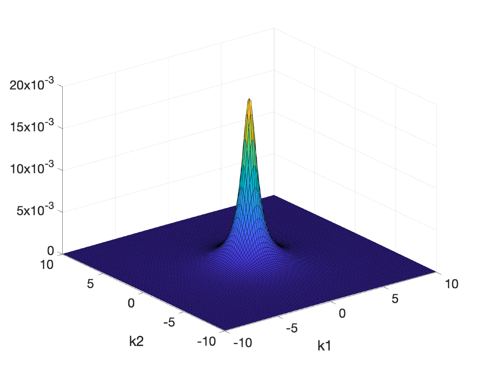
(a) Profile of stationary solution $f_{\text{eq}}$.

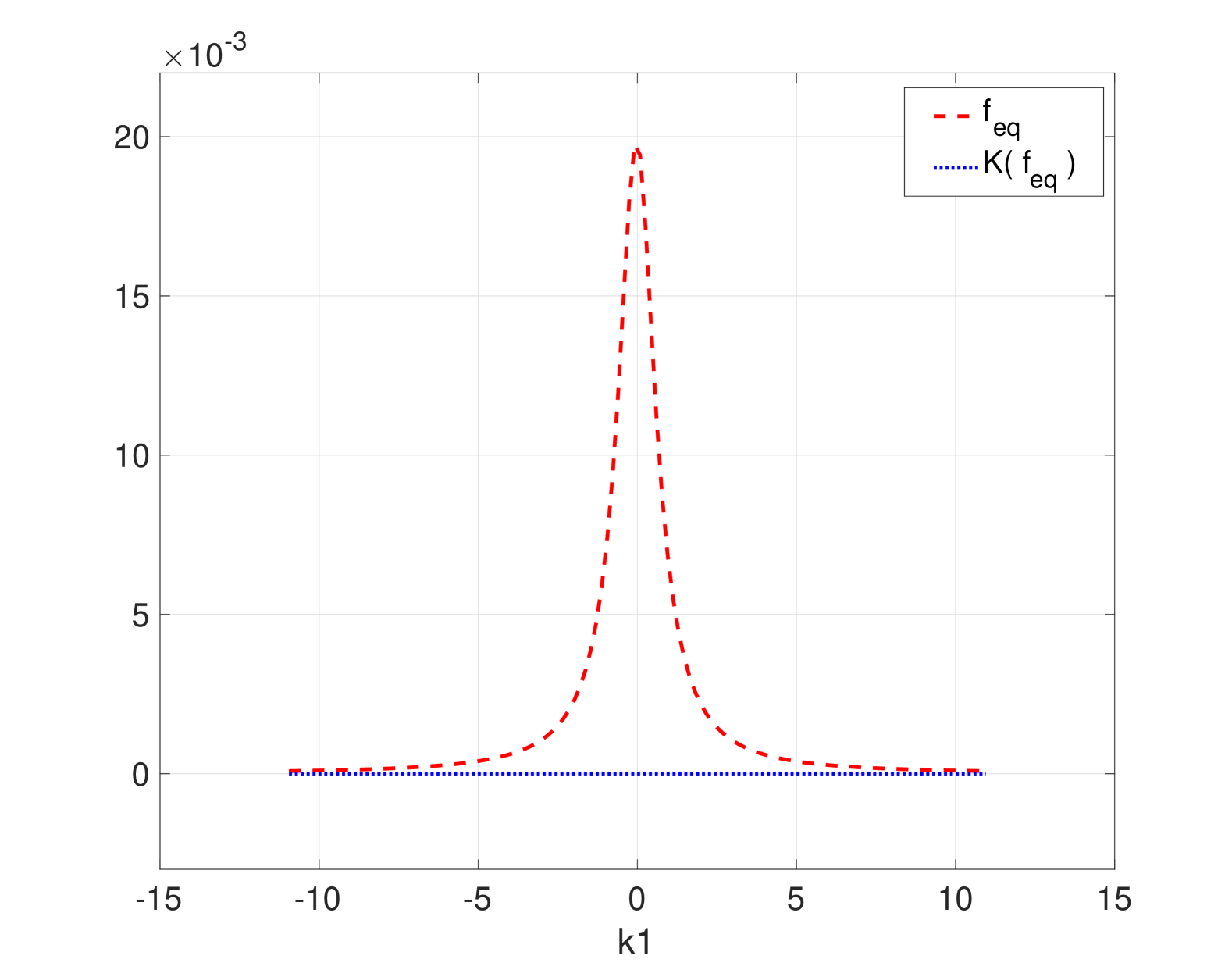
(b) $f_{\text{eq}}$ and $\mathcal{K}(f_{\text{eq}})$.

Figure 1: Stationary solution in 2D with $S=5,N_{r}=N=128,N_{s}=N_{sig}=12$.

4.1.2 Time evolution test in 2D

Now, we perform numerical tests for the 2D equation (1). The time discretization is performed by the fourth-order Runge-Kutta (RK4) methods.

Example 2 (Isotropic case). We consider the following isotropic initial condition:

(16) $$f^{0}(\mathbf{k})=\frac{1}{3}\left(\delta_{u}(|\mathbf{k}|)+\delta_{u}(|\mathbf{k}|-0.2)\right),$$

where $\delta_{u}(\mathbf{k})$ is an approximated delta function given by:

$$\delta_{u}(\mathbf{k})=\begin{cases}\frac{1}{2u}\left(1+\cos|\frac{\pi\mathbf{k}}{u}|\right),\quad&|\mathbf{k}|\leq u,\\[4.0pt] 0,&\text{otherwise}\,.\end{cases}$$

Here $u$ is taken to be $0.5\sqrt{\Delta\mathbf{k}}$ with $\Delta\mathbf{k}$ being the mesh size in $\mathbf{k}$. The time evolution of the solution in the top-to-bottom view is presented in Fig. 2. This numerical experiment is consistent with the theoretical result by Escobedo and Velázquez in [15, Section 1.1.1-1.1.2] that the WKE “generically” blows up, and in the form of a Dirac singularity.

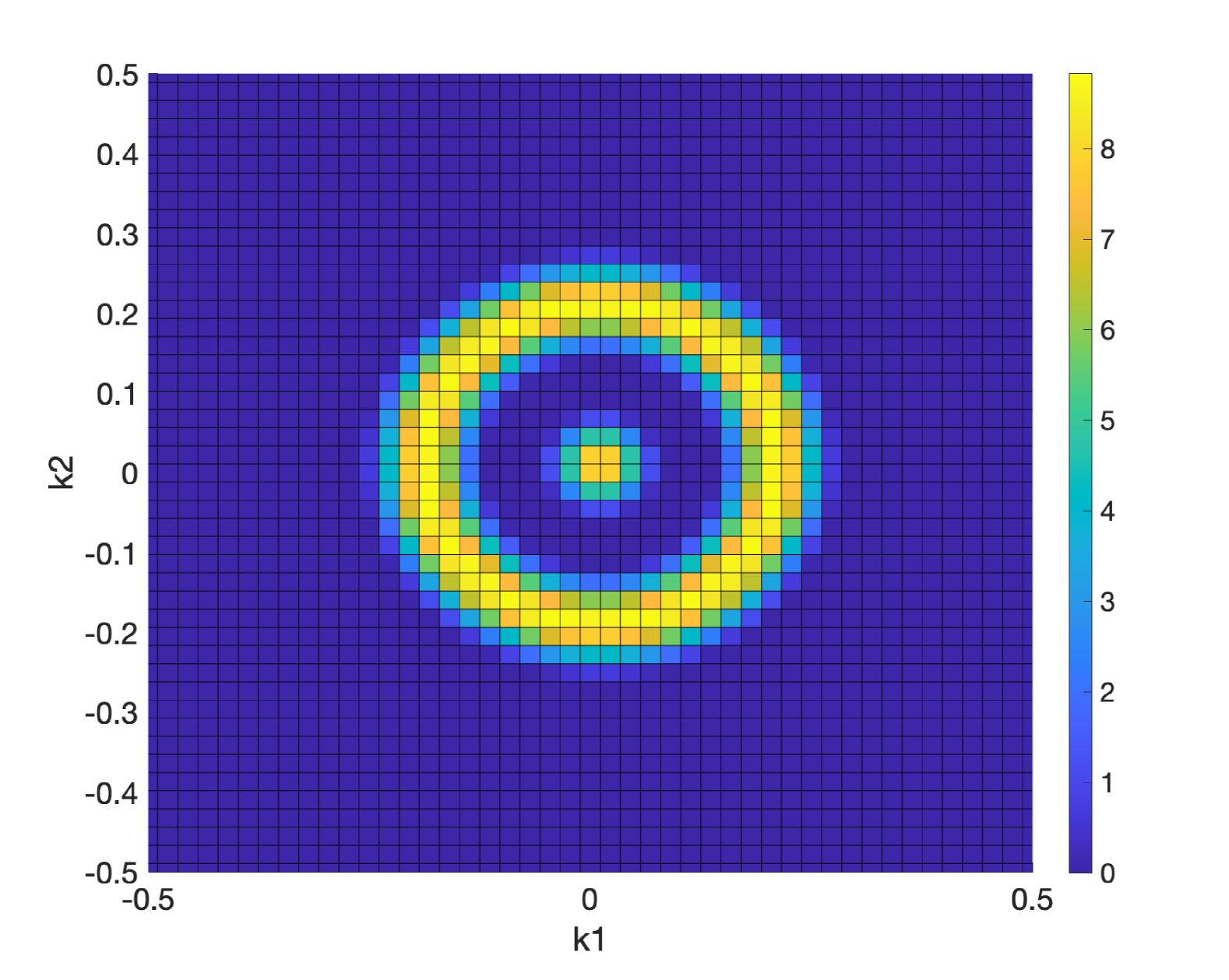
(a) t=0.0

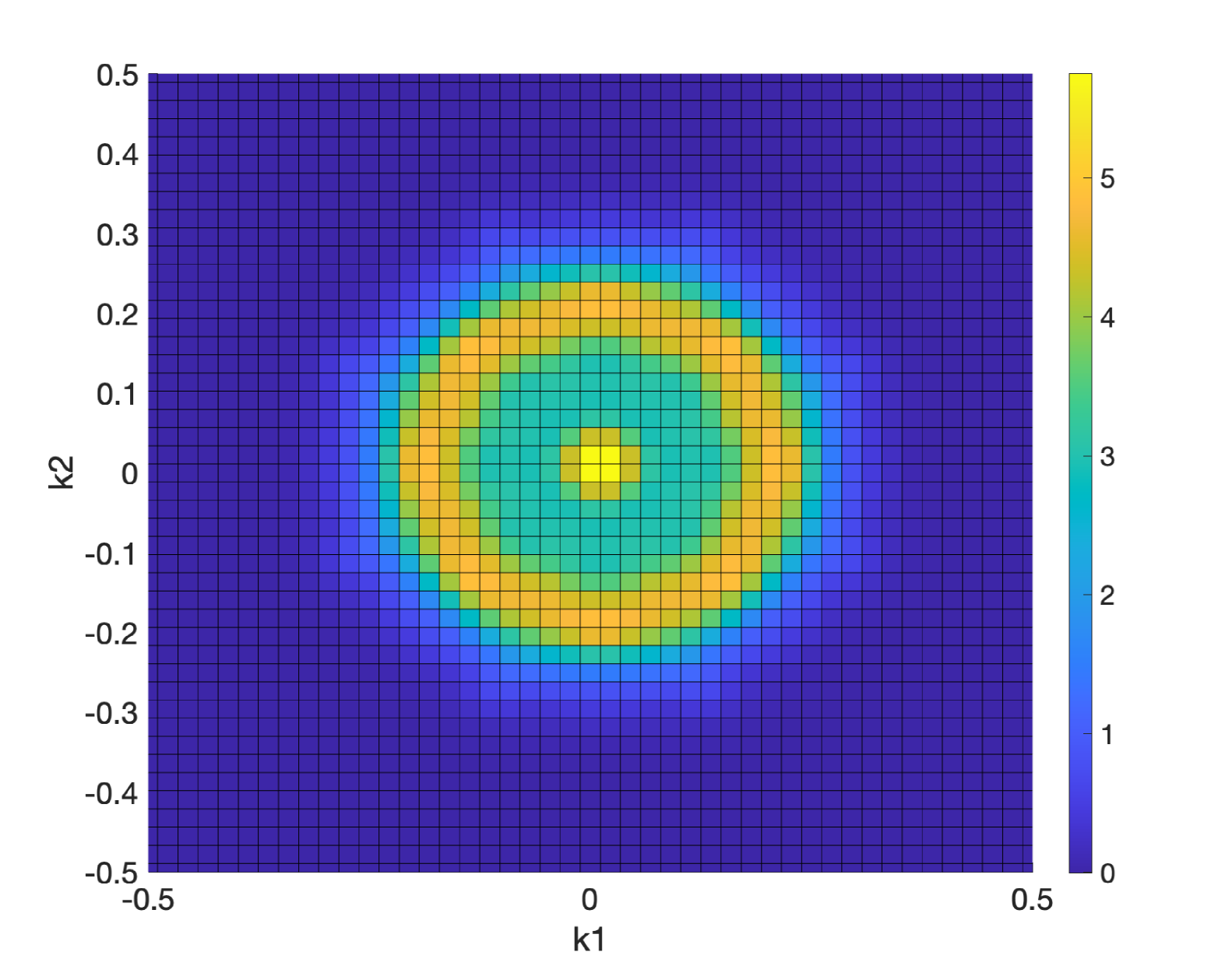
(b) t=0.2

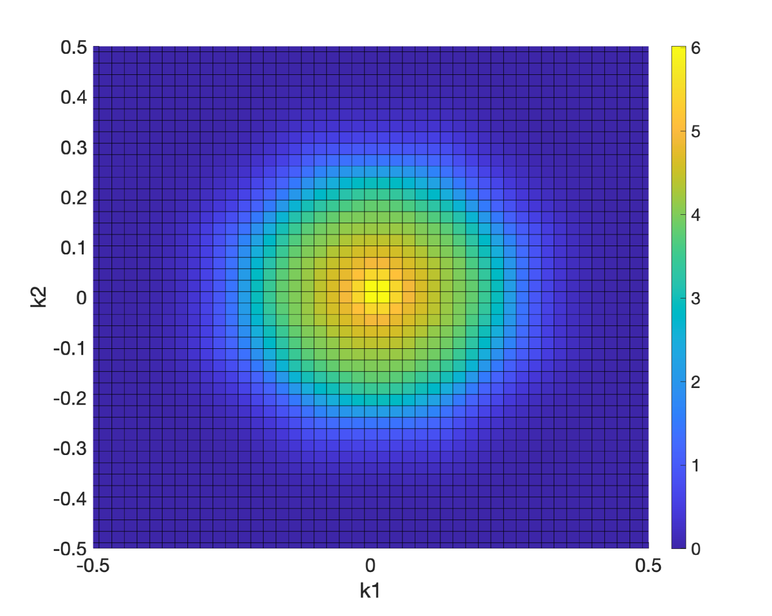
(c) t=0.4

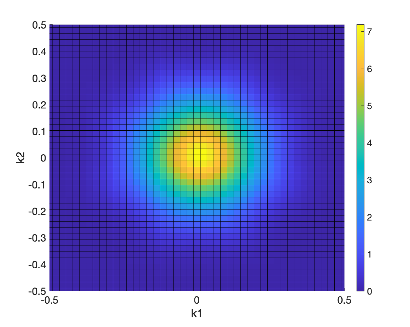
(d) t=0.6

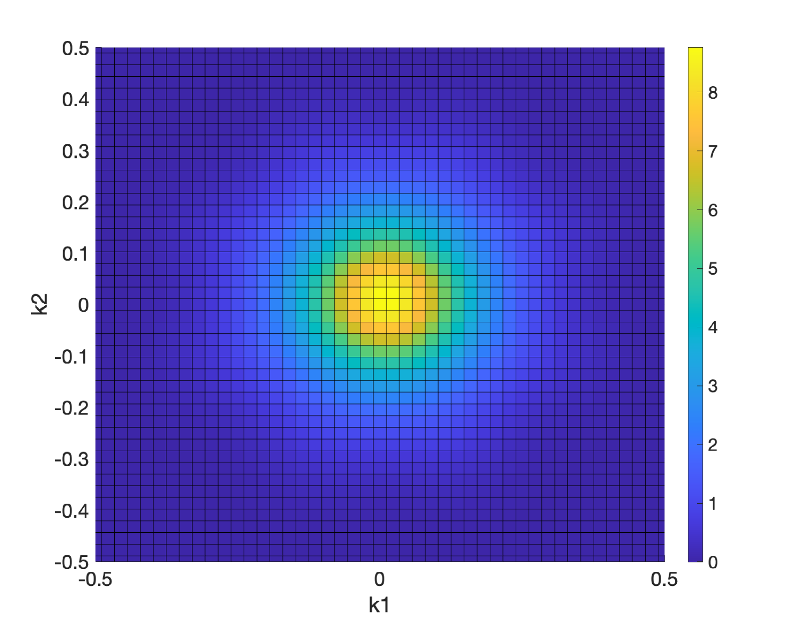
(e) t=0.8

(f) t=1.0

Figure 2: Top-to-bottom view of the time evolution of the solution profile for the isotropic initial condition (16) with $N_{r}=N=64,N_{s}=N_{sig}=12$, $S=0.33$ and $\Delta t=0.1$.

Example 3 (Discontinuous case). We consider the following discontinuous initial data in 2D:

(17) $$f^{0}_{\text{dis}}(\mathbf{k})=\begin{cases}\frac{\rho_{1}}{2\pi T_{1}}\exp\left(-\frac{|\mathbf{k}|^{2}}{2T_{1}}\right),\quad\text{for}\quad\mathbf{k}_{1}>0,\\[6.0pt] \frac{\rho_{2}}{2\pi T_{2}}\exp\left(-\frac{|\mathbf{k}|^{2}}{2T_{2}}\right),\quad\text{for}\quad\mathbf{k}_{1}<0,\end{cases}$$

where we pick $\rho_{1}=\frac{6}{5}$, $\rho_{2}=\frac{4}{5}$, $T_{1}=\frac{2}{3}$, $T_{2}=\frac{3}{2}$ such that

$$\rho(0)=\int_{\mathbb{R}^{2}}f^{0}_{\text{dis}}\,\mathrm{d}\mathbf{k}=1,\quad E(0)=\int_{\mathbb{R}^{2}}f^{0}_{\text{dis}}|\mathbf{k}|^{2}\,\mathrm{d}\mathbf{k}=2.$$

The profile of the discontinuous initial condition is drawn in Fig. 3.

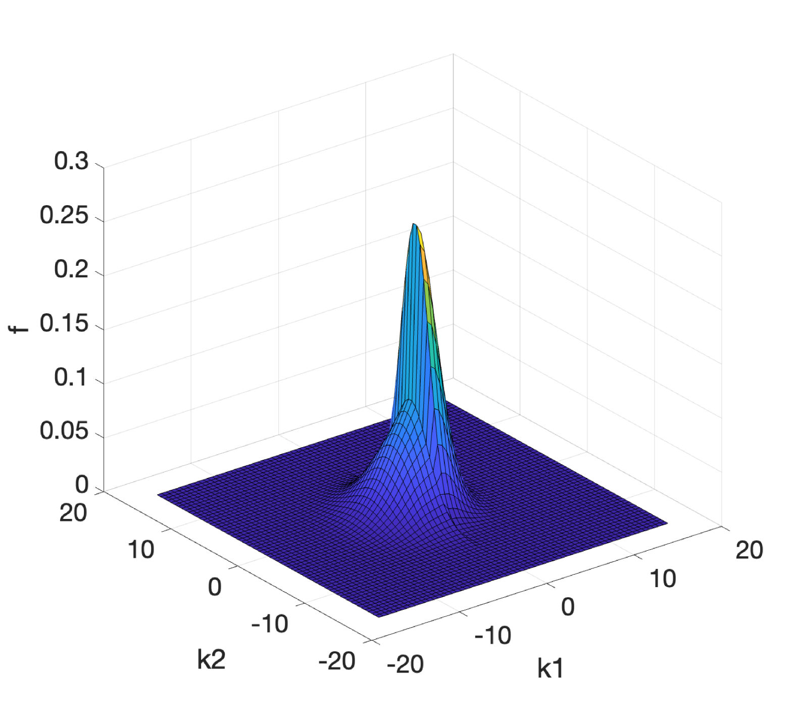
(a) Profile of $f^{0}_{\text{dis}}$

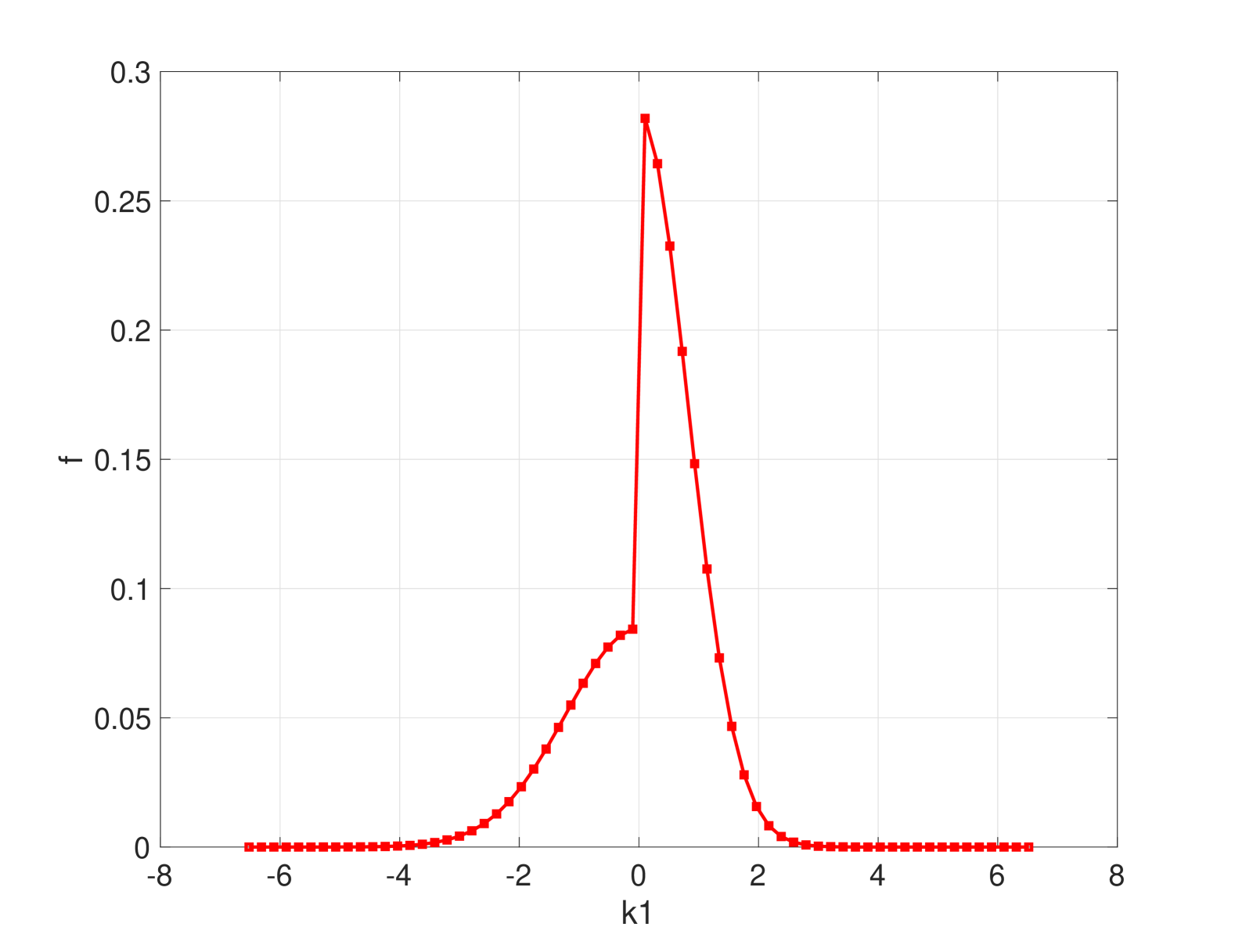
(b) Intersected profile of $f^{0}_{\text{dis}}(\mathbf{k}_{1},\mathbf{k}_{2}=0)$

Figure 3: Discontinous initial condition $f^{0}_{\text{dis}}$ in 2D for $N=N_{r}=64,N_{s}=N_{sig}=12$, $S=3$.

We use this example to check the conservation property of our method. This is shown in Fig. 4(a) and Fig. 4(b), where we present the conservation of the mass and energy over time.

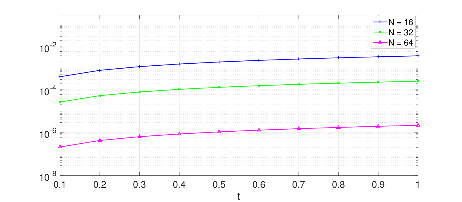
(a) Mass conservation $|\rho(t)-\rho(0)|$ in 2D.

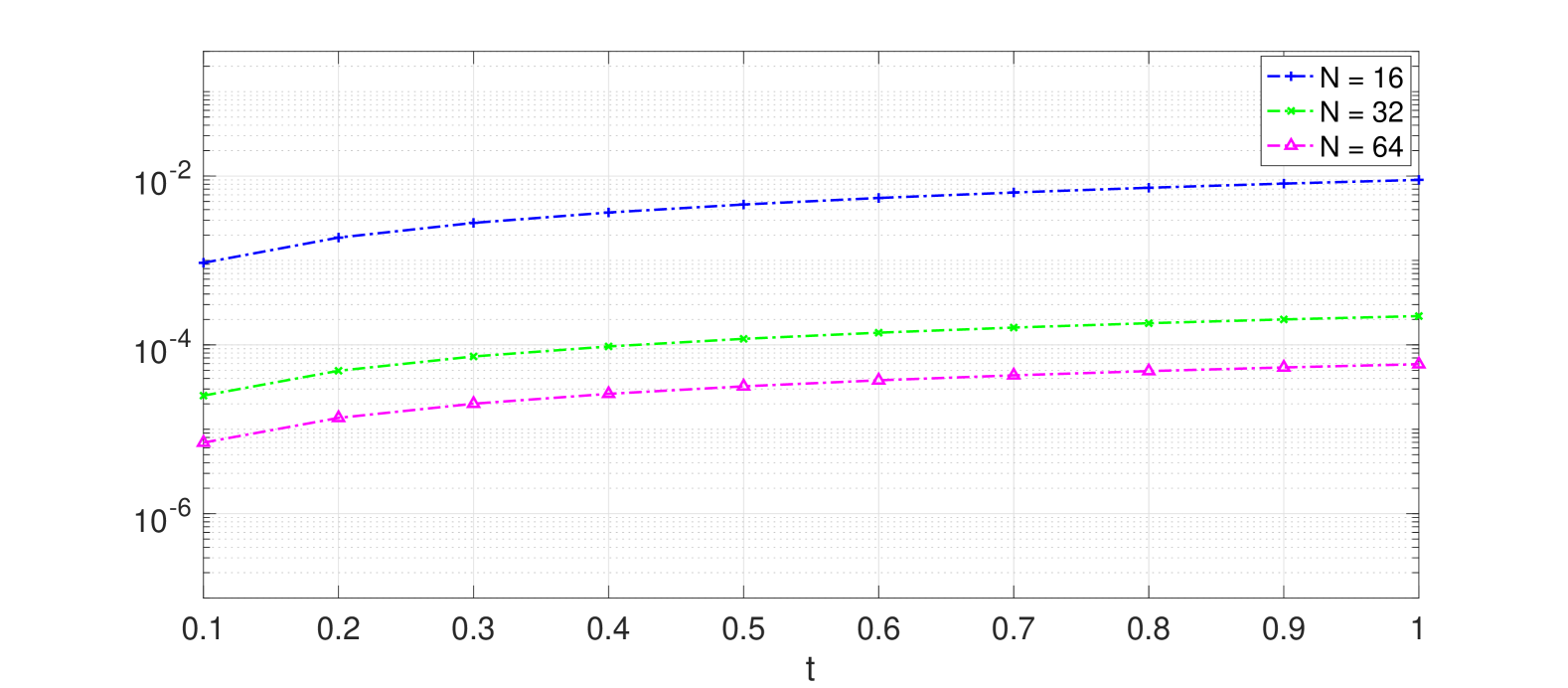
(b) Energy conservation $|E(t)-E(0)|$ in 2D.

Figure 4: Evolution of mass and energy in 2D for $N=N_{r},N_{s}=N_{sig}=12$ and $\Delta t=0.1$.

Example 4 (Non-isotropic case). In this example, we test a conjecture regarding the non-isotropic case. As discussed in the theoretical work [15, pp. 5-7] and demonstrated by the numerical experiment in Example 3, an isotropic initial condition can lead to a blow-up of the solution at the origin. It is conjectured that a non-isotropic initial condition will also lead to blow-up, but not symmetrically. In this test, we observe this phenomenon. As shown in Fig. 5, the solution evolves into a more concentrated profile; however, the center of the concentration does not remain at the origin, but shifts to a location dependent on the initial condition.

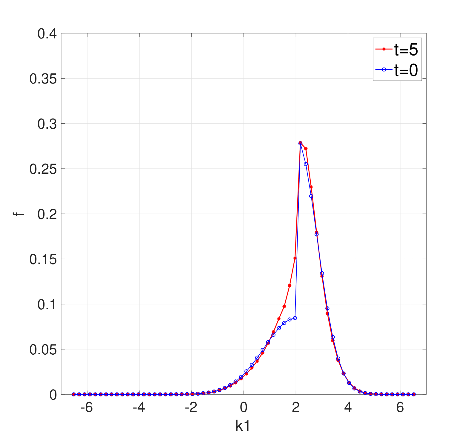
(a) t=5

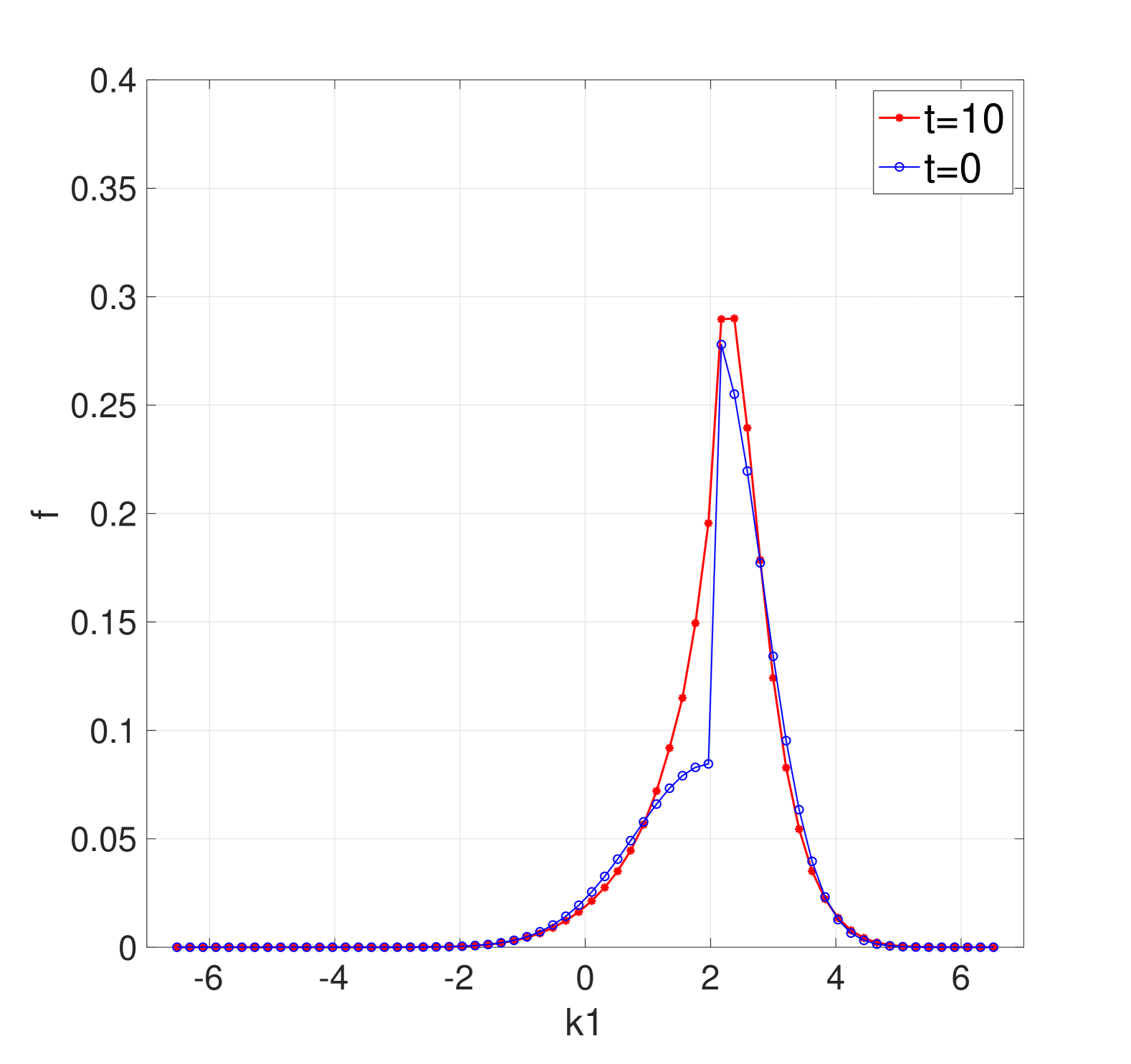
(b) t=10

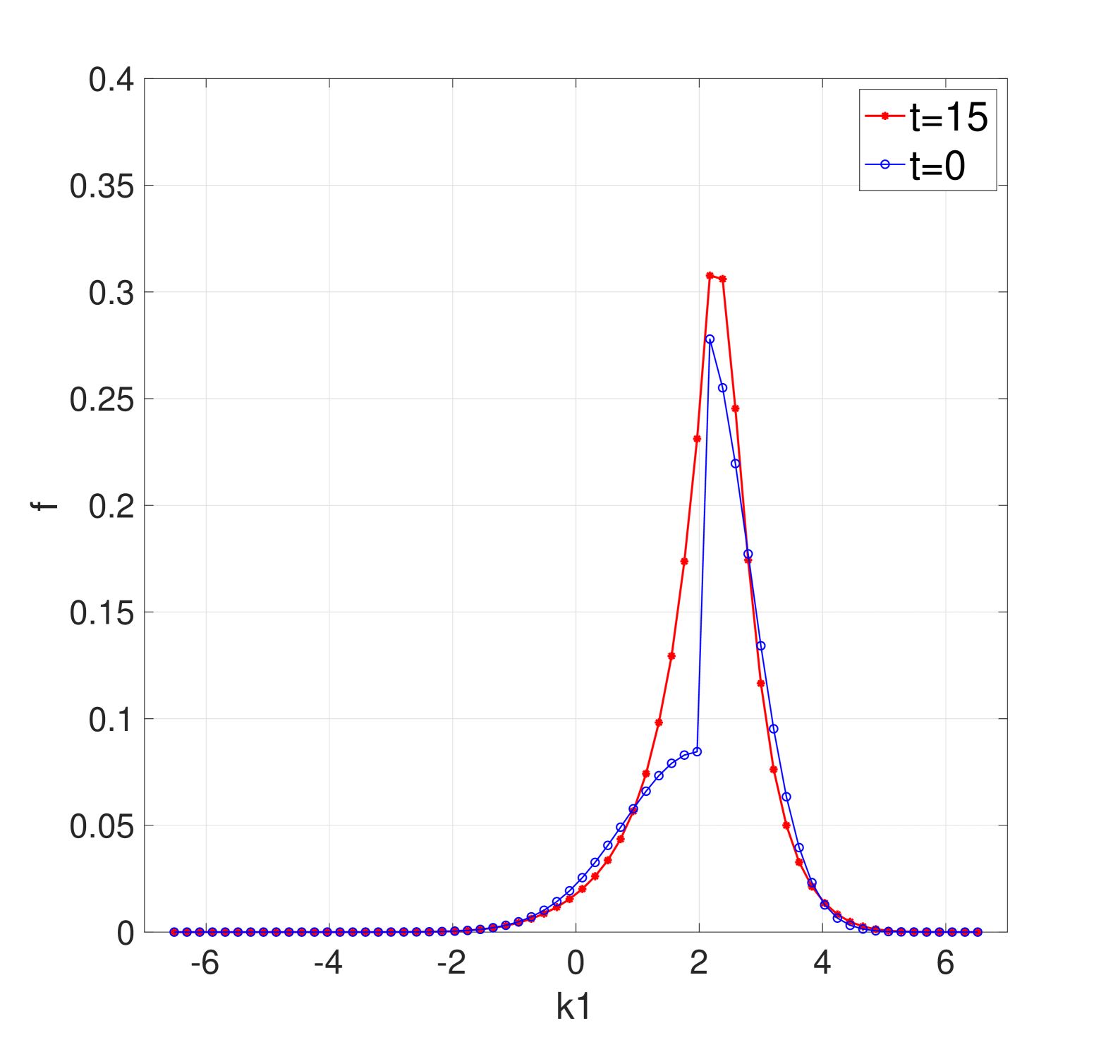
(c) t=15

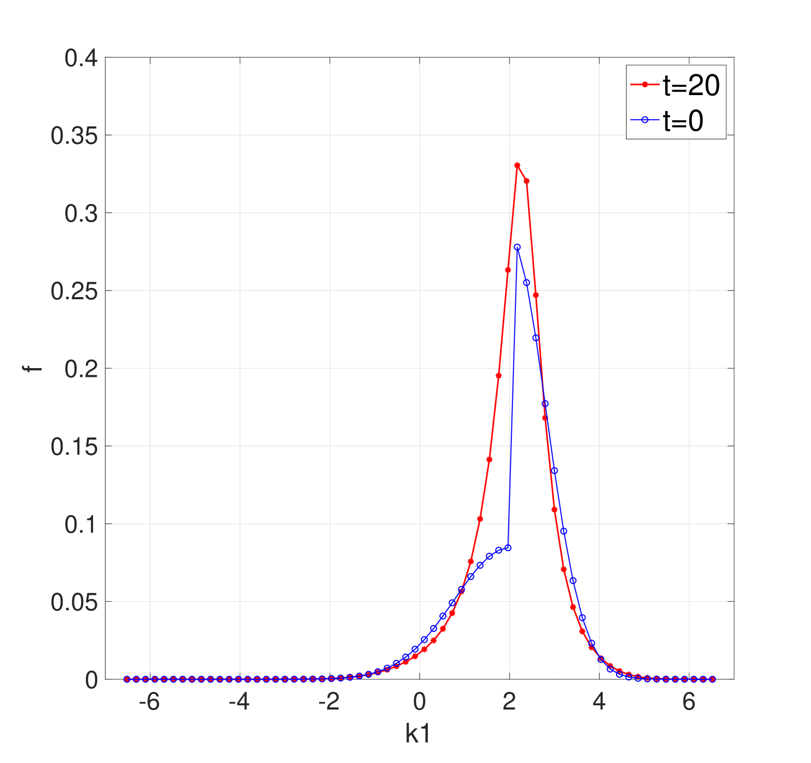
(d) t=20

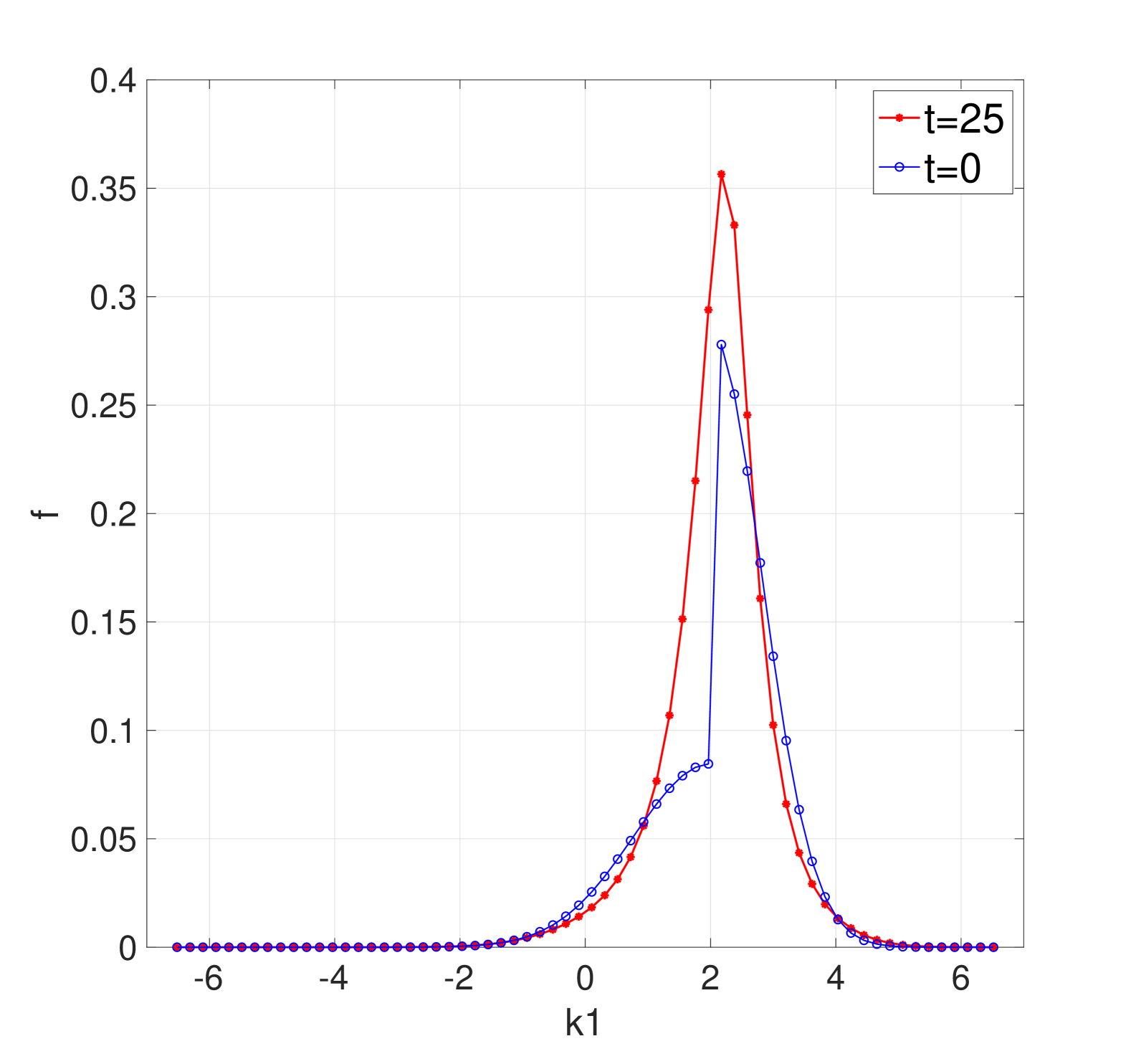
(e) t=25

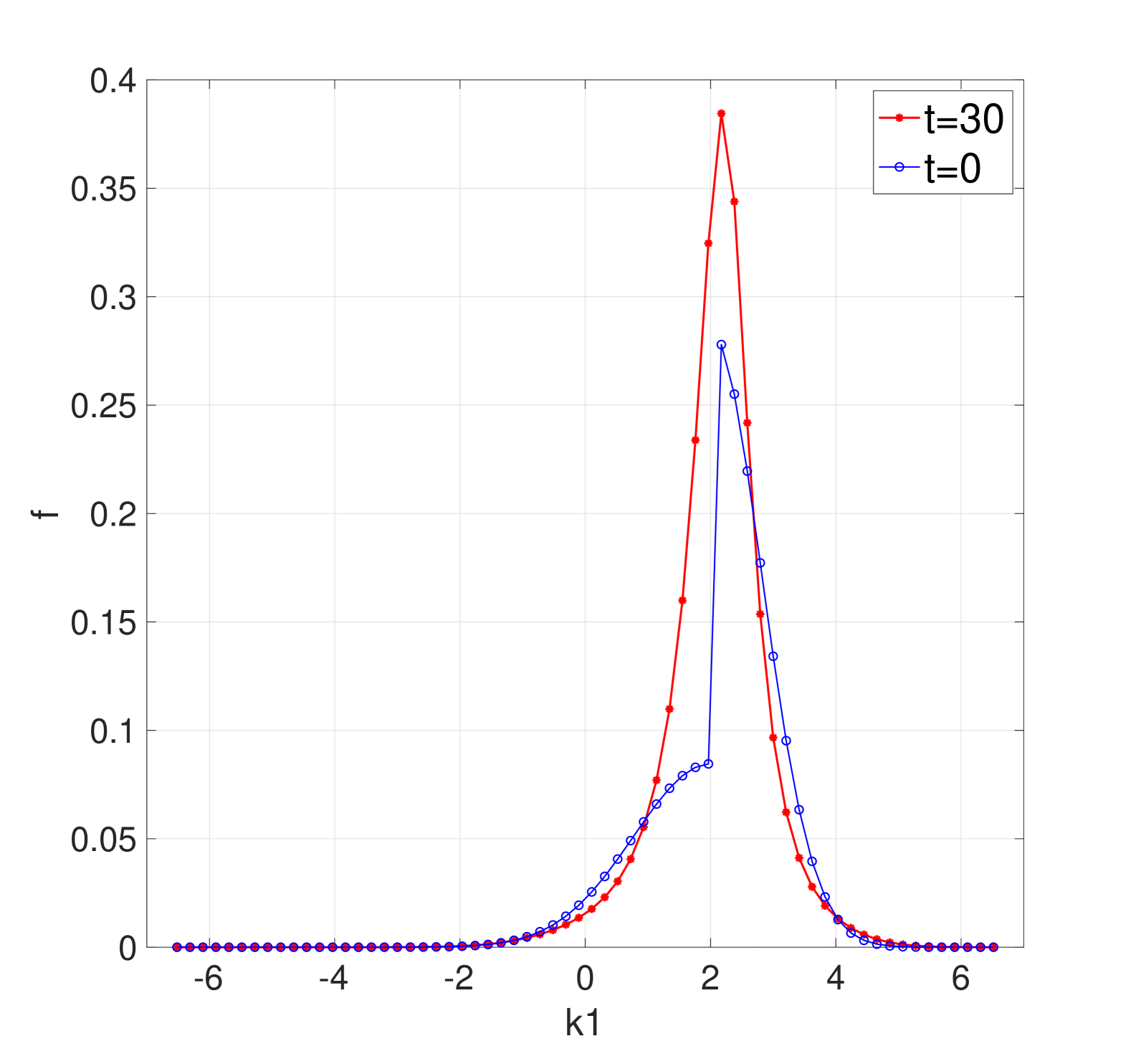
(f) t=30

Figure 5: Time evolution of the solution profile for the non-isotropic initial condition with $N=N_{r}=64,N_{s}=N_{sig}=8$, $S=3$ and $\Delta t=1$.

4.2 3D case

4.2.1 Stationary state test in 3D

Similar to the 2D case, we first use the stationary solution (5) to verify the accuracy of the method in 3D.

Example 5 (Stationary solution in 3D). Consider the specific stationary solution (5) in 3D with $\mu=10$, $\bm{\nu}=(5,5)$ and $\xi=20$. The $L^{\infty}$ and $L^{2}$ errors $\mathcal{K}(f_{\text{eq}})$ are presented in Table 2, while the associated computation time for each components: $\mathcal{K}_{1}$, $\mathcal{K}_{2}$, $\mathcal{K}_{3}$ and $\mathcal{K}_{4}$, are recorded in Table 3.

$N$	$\|\mathcal{K}(f_{\text{eq}})\|_{L^{\infty}}$	$\|\mathcal{K}(f_{\text{eq}})\|_{L^{2}}$
$16$	$1.7066\times 10^{-4}$	$1.7286\times 10^{-6}$
$32$	$1.2351\times 10^{-4}$	$1.9602\times 10^{-7}$
$64$	$7.2131\times 10^{-6}$	$5.4791\times 10^{-8}$

$N$	$\|\mathcal{K}(f_{\text{eq}})\|_{L^{\infty}}$	$\|\mathcal{K}(f_{\text{eq}})\|_{L^{2}}$
$16$	$1.9689\times 10^{-4}$	$7.2831\times 10^{-7}$
$32$	$6.8742\times 10^{-5}$	$4.9058\times 10^{-8}$
$64$	$5.0208\times 10^{-6}$	$9.9046\times 10^{-9}$

Table 2: $L^{\infty}$ and $L^{2}$ error of stationary solution in 3D for $N_{s}=6$ (left) and $N_{s}=12$ (right) with $N_{s}=N_{sig}=6$ and $S=5$.

	$\mathcal{K}_{1}$	$\mathcal{K}_{2}$	$\mathcal{K}_{3}$	$\mathcal{K}_{4}$	$\mathcal{K}$
$N=16$	$0.27$s	$0.17$s	$0.20$s	$0.18$s	$0.82$s
$N=32$	$2.11$s	$1.45$s	$1.60$s	$1.39$s	$6.55$s
$N=64$	$22.38$s	$14.67$s	$17.73$s	$16.21$s	$70.99$s

Table 3: Computational time in 3D for $N_{r}=N,N_{s}=N_{sig}=6$ and $S=5$.

4.2.2 Time evolution test in 3D

We then solve the time dependent problem (1) in 3D. Time discretization is again performed using the fourth-order Runge-Kutta (RK4) method.

Example 6 (Mass and energy conservation in 3D). Here we consider the same discontinuous initial condition (17) in 3D. The mass and energy evolution is presented in Fig. 6.

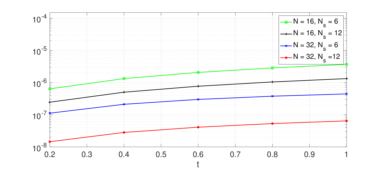
(a) Mass conservation $|\rho(t)-\rho(0)|$ in 3D

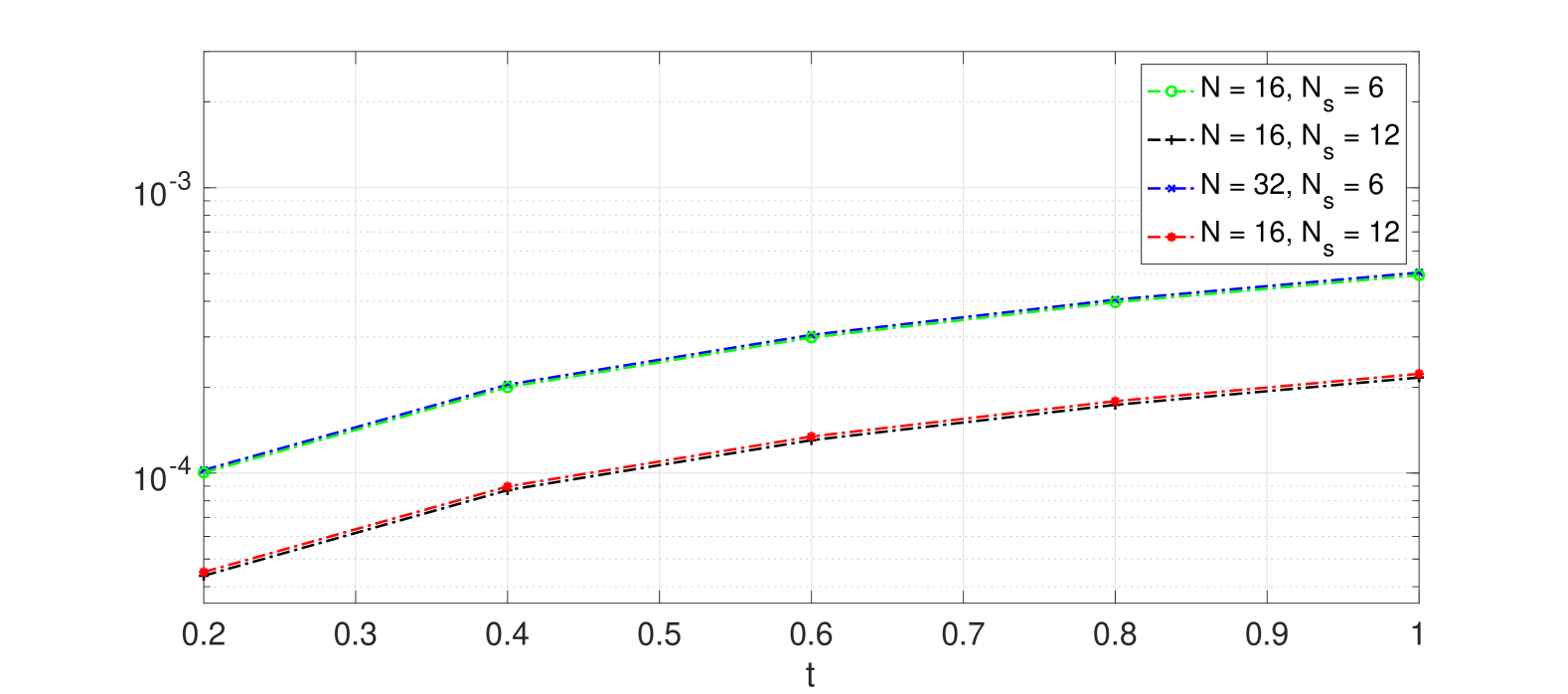
(b) Energy conservation $|E(t)-E(0)|$ in 3D

Figure 6: Evolution of mass and energy in 3D for $N=N_{r},N_{s}=N_{sig}$, $S=0.33$ and $\Delta t=0.1$.

5 Conclusion

In this work, we develop a fast Fourier spectral method for solving the wave kinetic equation (WKE), which arises as the kinetic limit of the cubic Schrödinger equation. The core idea of our approach is to reformulate the high-dimensional nonlinear wave kinetic operator as a spherical integral, drawing an analogy to the classical Boltzmann collision operator. Additionally, we extract a double-convolution structure from the numerical system by applying Fourier spectral approximation to the solution, enabling the use of the fast Fourier transform (FFT) to significantly enhance computational efficiency. This FFT-based approach not only accelerates computation but also eliminates the need for pre-computation and additional storage, making it a practical and scalable solution for high-dimensional problems.

While our approach borrows key ideas from previous works [29, 25], its application to the wave kinetic equation (WKE) is novel and could have a significant impact. Compared to earlier methods for computing the WKE, such as the Discrete Interaction Approximation (DIA) [21] and quadrature-based approaches (e.g., the WRT method) [42, 39], our method excels in both accuracy and efficiency. Through a series of numerical experiments in 2D and 3D, we demonstrate the performance of the proposed method in both steady-state and time-evolving scenarios, including isotropic and non-isotropic cases. These results highlight the potential of our method as a robust and efficient tool for simulating wave kinetic dynamics within wave turbulence theory.

Appendix A Reformulation of WKE in form of classical Boltzmann-type equation

In this appendix, we present the derivation reformulating the form (3) as an integral over a sphere, leading to the usual form of Boltzmann-type collision operator as in (6).

Step I: Denote $\mathbf{O}=\frac{(\mathbf{k}_{1}+\mathbf{k}_{3})}{2}$ and $\mathbf{P}=\frac{(\mathbf{k}_{1}-\mathbf{k}_{3})}{2}$ such that

$$\mathbf{k}_{1}=\mathbf{O}+\mathbf{P},\quad\mathbf{k}_{3}=\mathbf{O}-\mathbf{P},$$

and applying the change of variable $(\mathbf{k}_{1},\mathbf{k}_{3})\mapsto(\mathbf{O},\mathbf{P})$ with the Jacobian $2^{d}$ in (3), we have

$$\begin{split}\mathcal{K}(f,f,f)(\mathbf{k})=2^{d}&\int_{(\mathbb{R}^{d})^{3}}\Big{[}f(\mathbf{O}+\mathbf{P})f(\mathbf{k}_{2})f(\mathbf{O}-\mathbf{P})-f(\mathbf{k})f(\mathbf{k}_{2})f(\mathbf{O}-\mathbf{P})\\ &\quad+f(\mathbf{O}+\mathbf{P})f(\mathbf{k})f(\mathbf{O}-\mathbf{P})-f(\mathbf{O}+\mathbf{P})f(\mathbf{k}_{2})f(\mathbf{k})\Big{]}\\ &\times\delta\left(\mathbf{k}_{2}+\mathbf{k}-2\mathbf{O}\right)\times\delta\left(\frac{|\mathbf{k}_{2}|^{2}}{2}+\frac{|\mathbf{k}|^{2}}{2}-\mathbf{O}^{2}-\mathbf{P}^{2}\right)\,\mathrm{d}\mathbf{O}\,\mathrm{d}\mathbf{k}_{2}\,\mathrm{d}\mathbf{P}.\end{split}$$

Step II: Let $\mathbf{P}=\rho\bm{\sigma}$ with $\rho\in[0,\infty)$ and $\bm{\sigma}\in\mathbb{S}^{d-1}$, such that $\mathrm{d}\mathbf{P}=\rho^{d-1}\,\mathrm{d}\rho\,\mathrm{d}\bm{\sigma}$,

$$\begin{split}&\mathcal{K}(f,f,f)(\mathbf{k})=\\[4.0pt] &2^{d}\int_{(\mathbb{R}^{d})^{2}}\int_{\mathbb{S}^{d-1}}\int_{0}^{\infty}\Big{[}f(\mathbf{O}+\rho\bm{\sigma})f(\mathbf{k}_{2})f(\mathbf{O}-\rho\bm{\sigma})-f(\mathbf{k})f(\mathbf{k}_{2})f(\mathbf{O}-\rho\bm{\sigma})\\ &\quad+f(\mathbf{O}+\rho\bm{\sigma})f(\mathbf{k})f(\mathbf{O}-\rho\bm{\sigma})-f(\mathbf{O}+\rho\bm{\sigma})f(\mathbf{k}_{2})f(\mathbf{k})\Big{]}\\ &\times\delta\left(\mathbf{k}_{2}+\mathbf{k}-2\mathbf{O}\right)\times\delta\left(\frac{|\mathbf{k}_{2}|^{2}}{2}+\frac{|\mathbf{k}|^{2}}{2}-\mathbf{O}^{2}-\rho^{2}\right)\rho^{d-1}\,\mathrm{d}\rho\,\mathrm{d}\bm{\sigma}\,\mathrm{d}\mathbf{O}\,\mathrm{d}\mathbf{k}_{2},\end{split}$$

then, replacing $\rho^{2}$ by $=\frac{|\mathbf{k}_{2}|^{2}}{2}+\frac{|\mathbf{k}|^{2}}{2}-\mathbf{O}^{2}$, we obtain

$$\begin{split}\mathcal{K}&(f,f,f)(\mathbf{k})=\frac{1}{2}\int_{(\mathbb{R}^{d})^{2}}\int_{\mathbb{S}^{d-1}}\\ &\Bigg{[}f\left(\mathbf{O}+\sqrt{\frac{|\mathbf{k}_{2}|^{2}}{2}+\frac{|\mathbf{k}|^{2}}{2}-\mathbf{O}^{2}}\bm{\sigma}\right)f(\mathbf{k}_{2})f\left(\mathbf{O}-\sqrt{\frac{|\mathbf{k}_{2}|^{2}}{2}+\frac{|\mathbf{k}|^{2}}{2}-\mathbf{O}^{2}}\bm{\sigma}\right)\\ &-f(\mathbf{k})f(\mathbf{k}_{2})f\left(\mathbf{O}-\sqrt{\frac{|\mathbf{k}_{2}|^{2}}{2}+\frac{|\mathbf{k}|^{2}}{2}-\mathbf{O}^{2}}\bm{\sigma}\right)\\ &+f\left(\mathbf{O}+\sqrt{\frac{|\mathbf{k}_{2}|^{2}}{2}+\frac{|\mathbf{k}|^{2}}{2}-\mathbf{O}^{2}}\bm{\sigma}\right)f(\mathbf{k})f\left(\mathbf{O}-\sqrt{\frac{|\mathbf{k}_{2}|^{2}}{2}+\frac{|\mathbf{k}|^{2}}{2}-\mathbf{O}^{2}}\bm{\sigma}\right)\\ &-f\left(\mathbf{O}+\sqrt{\frac{|\mathbf{k}_{2}|^{2}}{2}+\frac{|\mathbf{k}|^{2}}{2}-\mathbf{O}^{2}}\bm{\sigma}\right)f(\mathbf{k}_{2})f(\mathbf{k})\Bigg{]}\\ &\times\delta\left(\mathbf{O}-\frac{\mathbf{k}_{2}+\mathbf{k}}{2}\right)\times\left(\frac{|\mathbf{k}_{2}|^{2}}{2}+\frac{|\mathbf{k}|^{2}}{2}-\mathbf{O}^{2}\right)^{\frac{d-2}{2}}\,\mathrm{d}\bm{\sigma}\,\mathrm{d}\mathbf{O}\,\mathrm{d}\mathbf{k}_{2}.\end{split}$$

Step III: By integration over $\mathbf{O}$ (replacing $\mathbf{O}$ by $=\frac{\mathbf{k}_{2}+\mathbf{k}}{2}$ above) and considering the fact that

$$\sqrt{\frac{|\mathbf{k}_{2}|^{2}}{2}+\frac{|\mathbf{k}|^{2}}{2}-\mathbf{O}^{2}}=\frac{|\mathbf{k}-\mathbf{k}_{2}|}{2},$$

we obtain

$$\begin{split}\mathcal{K}(f,f,f)=&\frac{1}{2}\int_{\mathbb{R}^{d}}\int_{\mathbb{S}^{d-1}}\Bigg{[}f\left(\frac{\mathbf{k}_{2}+\mathbf{k}}{2}+\frac{|\mathbf{k}-\mathbf{k}_{2}|}{2}\bm{\sigma}\right)f(\mathbf{k}_{2})f\left(\frac{\mathbf{k}_{2}+\mathbf{k}}{2}-\frac{|\mathbf{k}-\mathbf{k}_{2}|}{2}\bm{\sigma}\right)\\[3.0pt] &-f(\mathbf{k})f(\mathbf{k}_{2})f\left(\frac{\mathbf{k}_{2}+\mathbf{k}}{2}-\frac{|\mathbf{k}-\mathbf{k}_{2}|}{2}\bm{\sigma}\right)\\[3.0pt] &+f\left(\frac{\mathbf{k}_{2}+\mathbf{k}}{2}+\frac{|\mathbf{k}-\mathbf{k}_{2}|}{2}\bm{\sigma}\right)f(\mathbf{k})f\left(\frac{\mathbf{k}_{2}+\mathbf{k}}{2}-\frac{|\mathbf{k}-\mathbf{k}_{2}|}{2}\bm{\sigma}\right)\\[3.0pt] &-f\left(\frac{\mathbf{k}_{2}+\mathbf{k}}{2}+\frac{|\mathbf{k}-\mathbf{k}_{2}|}{2}\bm{\sigma}\right)f(\mathbf{k}_{2})f(\mathbf{k})\Bigg{]}\\[3.0pt] &\times\left(\frac{|\mathbf{k}-\mathbf{k}_{2}|}{2}\right)^{d-2}\,\mathrm{d}\bm{\sigma}\,\mathrm{d}\mathbf{k}_{2},\end{split}$$

which, by denoting

$$\frac{\mathbf{k}_{2}+\mathbf{k}}{2}+\frac{|\mathbf{k}-\mathbf{k}_{2}|}{2}\bm{\sigma}=:\mathbf{k}^{\prime},\quad\frac{\mathbf{k}_{2}+\mathbf{k}}{2}-\frac{|\mathbf{k}-\mathbf{k}_{2}|}{2}\bm{\sigma}=:\mathbf{k}^{\prime}_{2}\,,$$

can finally be written as in (6).

References

• [1] A. M. Balk and V. E. Zakharov, Stability of weak-turbulence Kolmogorov spectra, in Nonlinear waves and weak turbulence, vol. 182 of Amer. Math. Soc. Transl. Ser. 2, Amer. Math. Soc., Providence, RI, 1998, pp. 31–81.
• [2] J. W. Banks, T. Buckmaster, A. O. Korotkevich, G. Kovacic, and J. Shatah, Direct verification of the kinetic description of wave turbulence for finite-size systems dominated by interactions among groups of six waves, Phys. Rev. Lett., 129 (2022), pp. Paper No. 034101, 6.
• [3] T. Buckmaster, P. Germain, Z. Hani, and J. Shatah, On the kinetic wave turbulence description for NLS, Quart. Appl. Math., 78 (2020), pp. 261–275.
• [4] T. Buckmaster, P. Germain, Z. Hani, and J. Shatah, Onset of the wave turbulence description of the longtime behavior of the nonlinear Schrödinger equation, Invent. Math., 225 (2021), pp. 787–855.
• [5] C. Collot, H. Dietert, and P. Germain, Stability and cascades for the Kolmogorov-Zakharov spectrum of wave turbulence, Arch. Ration. Mech. Anal., 248 (2024), pp. Paper No. 7, 31.
• [6] C. Collot and P. Germain, On the derivation of the homogeneous kinetic wave equation, preprint, arXiv:1912.10368, (2019).
• [7] C. Collot and P. Germain, Derivation of the homogeneous kinetic wave equation: longer time scales, preprint, arXiv:2007.03508, (2020).
• [8] Y. Deng and Z. Hani, On the derivation of the wave kinetic equation for NLS, Forum Math. Pi, 9 (2021), pp. Paper No. e6, 37.
• [9] Y. Deng and Z. Hani, Full derivation of the wave kinetic equation, Invent. Math., 233 (2023), pp. 543–724.
• [10] Y. Deng and Z. Hani, Long time justification of wave turbulence theory, preprint, arXiv:2311.10082, (2024).
• [11] G. Dimarco and L. Pareschi, Numerical methods for kinetic equations, Acta Numer., 23 (2014), pp. 369–520.
• [12] S. Dyachenko, A. Newell, A. Pushkarev, and V. Zakharov, Optical turbulence: weak turbulence, condensates and collapsing filaments in the nonlinear schrödinger equation, Physica D: Nonlinear Phenomena, 57 (1992), pp. 96–160.
• [13] M. Escobedo and A. Menegaki, Instability of singular equilibria of a wave kinetic equation, preprint, arXiv:2406.05280, (2024).
• [14] M. Escobedo and J. J. L. Velázquez, Finite time blow-up and condensation for the bosonic Nordheim equation, Invent. Math., 200 (2015), pp. 761–847.
• [15] M. Escobedo and J. J. L. Velázquez, On the theory of weak turbulence for the nonlinear Schrödinger equation, Mem. Amer. Math. Soc., 238 (2015), pp. v+107.
• [16] F. Filbet, J. Hu, and S. Jin, A numerical scheme for the quantum Boltzmann equation with stiff collision terms, ESAIM: Math. Model. Numer. Anal. (M2AN), 46 (2012), pp. 443–463.
• [17] F. Filbet, C. Mouhot, and L. Pareschi, Solving the Boltzmann equation in NlogN, SIAM J. Sci. Comput., 28 (2006), pp. 1029–1053.
• [18] F. Filbet and G. Russo, High order numerical methods for the space non-homogeneous Boltzmann equation, J. Comput. Phys., 186 (2003), pp. 457–480.
• [19] I. Gamba, J. Haack, C. Hauck, and J. Hu, A fast spectral method for the Boltzmann collision operator with general collision kernels, SIAM J. Sci. Comput., 39 (2017), pp. B658–B674.
• [20] P. Germain, A. D. Ionescu, and M.-B. Tran, Optimal local well-posedness theory for the kinetic wave equation, J. Funct. Anal., 279 (2020), pp. 108570, 28.
• [21] S. Hasselmann, K. Hasselmann, J. Allender, and T. Barnett, Computations and parameterizations of the nonlinear energy transfer in a gravity-wave specturm. part ii: Parameterizations of the nonlinear energy transfer for application in wave models, Journal of Physical Oceanography, 15 (1985), pp. 1378–1391.
• [22] J. Hu and K. Qi, A fast Fourier spectral method for the homogeneous Boltzmann equation with non-cutoff collision kernels, J. Comput. Phys., 423 (2020), p. 109806.
• [23] J. Hu, K. Qi, and T. Yang, A new stability and convergence proof of the Fourier-Galerkin spectral method for the spatially homogeneous Boltzmann equation, SIAM J. Numer. Anal., 59 (2021), pp. 613–633.
• [24] J. Hu and L. Ying, A fast spectral algorithm for the quantum Boltzmann collision operator, Commun. Math. Sci., 10 (2012), pp. 989–999.
• [25] J. Hu and L. Ying, A fast algorithm for the energy space boson Boltzmann collision operator, Math. Comp., 84 (2015), pp. 271–288.
• [26] P. Janssen, The interaction of ocean waves and wind, Cambridge University Press, 2004.
• [27] J. Lukkarinen and H. Spohn, Weakly nonlinear Schrödinger equation with random initial data, Invent. Math., 183 (2011), pp. 79–188.
• [28] A. Menegaki, $L^{2}$-stability near equilibrium for the 4 waves kinetic equation, Kinet. Relat. Models, 17 (2024), pp. 514–532.
• [29] C. Mouhot and L. Pareschi, Fast algorithms for computing the Boltzmann collision operator, Math. Comp., 75 (2006), pp. 1833–1852.
• [30] S. Nazarenko, Wave turbulence, vol. 825, Springer, 2011.
• [31] A. C. Newell and B. Rumpf, Wave turbulence, Annual review of fluid mechanics, 43 (2011), pp. 59–78.
• [32] L. Pareschi and B. Perthame, A Fourier spectral method for homogeneous Boltzmann equations, Transport Theory Statist. Phys., 25 (1996), pp. 369–382.
• [33] L. Pareschi and G. Russo, Numerical solution of the Boltzmann equation I: spectrally accurate approximation of the collision operator, SIAM J. Numer. Anal., 37 (2000), pp. 1217–1245.
• [34] L. Pareschi, G. Russo, and G. Toscani, Fast spectral methods for the Fokker-Planck-Landau collision operator, J. Comput. Phys., 165 (2000), pp. 216–236.
• [35] D. Resio and W. Perrie, A numerical study of nonlinear energy fluxes due to wave-wave interactions part 1. methodology and basic results, J. Fluid Mech., 223 (1991), pp. 603–629.
• [36] B. V. Semisalov, S. B. Medvedev, S. V. Nazarenko, and M. P. Fedoruk, Algorithm for solving the four-wave kinetic equation in problems of wave turbulence, Comput. Math. Math. Phys., 64 (2024), pp. 340–361.
• [37] G. Staffilani and M.-B. Tran, Condensation and non-condensation times for 4-wave kinetic equations, preprint, arXiv:2407.18533, (2024).
• [38] G. Staffilani and M.-B. Tran, On the energy transfer towards large values of wavenumbers for solutions of 4-wave kinetic equations, preprint, arXiv:2407.18508, (2024).
• [39] B. A. Tracy and D. T. Resio, Theory and calculation of the nonlinear energy transfer between sea waves in deep water, in Proceedings of the Army Numerical and Computers Analysis Conference, US Army Research Office., 1982, p. 457.
• [40] S. Walton and M.-B. Tran, A numerical scheme for wave turbulence: 3-wave kinetic equations, SIAM J. Sci. Comput., 45 (2023), pp. B467–B492.
• [41] S. Walton, M.-B. Tran, and A. Bensoussan, A deep learning approximation of non-stationary solutions to wave kinetic equations, Appl. Numer. Math., 199 (2024), pp. 213–226.
• [42] D. J. Webb, Non-linear transfers between sea waves, Deep Sea Research, 25 (1978), pp. 279–298.
• [43] R. Womersley, Symmetric Spherical Designs on the sphere $S^{2}$ with good geometric properties, The University of New South Wales., http://web.maths.unsw.edu.au/~rsw/Sphere/EffSphDes/ss.html (accessed Sep. 27, 2016).
• [44] V. Zakharov and N. Filonenko, Weak turbulence of capillary waves, Journal of applied mechanics and technical physics, 8 (1967), pp. 37–40.
• [45] V. E. Zakharov, V. S. L’vov, and G. Falkovich, Kolmogorov spectra of turbulence I: Wave turbulence, Springer Science & Business Media, 2012.