A study of the Antlion Random Walk

Abstract

This paper treats a new type of random walk referred to as an Antlion Random Walk (ARW), which is motivated by mathematical modeling of the decision-making process using chaotic semiconductor lasers with memory parameters. We discuss the dependency of the property of the probability distribution of ARWs on the memory parameter $\alpha$ and discuss uniqueness of them in contrast to the conventional, simple RWs through similarity to the normal distribution.

1 Introduction

A Random Walk (RW) [1] is one of the most fundamental concepts of the stochastic process, which describes a path consisting of a succession of random steps. It is a key concept in probability theory and is widely applied in various fields, including physics [2], finance [3], economics [4, 5]. In particular, RW is a fundamental scheme to construct algorithms that treat stochastic state transition in the realm of computer science [6]. In its simplest form, RW describes movement in a discrete one-dimensional lattice labeled by integers in order of unit steps, which we call simple RW in this paper. However, this model also has many variations tailored to different applications’ requirements; it can be extended in terms of dimensionality, step length, time continuity, etc. This paper provides a new type of extension on retaining history, which initially attracted attention for the theoretical construction of a decision-making system using chaotic phenomena.

Chaotic phenomena exhibit behaviors that make them appear random and unpredictable over long periods, and their practical unpredictability is often statistically addressed using probability theory [7]. These statistical properties of chaotic phenomena lead to fruitful applications [8], including the creation of a physical random number generator by chaotic semiconductor lasers [9, 10]. Moreover, their subsequent applications to decision-making systems are also presented, named after laser chaos decision-maker [11, 12]. Herein, one considers the multi-armed bandit (MAB) problem [13], or one of the simplest settings for reinforcement learning [14], which optimizes the repeated selections of multiple slot machines (or arm) that probabilistically gives a reward. The criterion of the laser chaos decision-maker is based on the tug-of-war model [15], which is inspired by the fluctuation or the probabilistic behavior of the body of slime molds. It has been experimentally clarified that the physical implementation of the tug-of-war method by chaotic phenomena by semiconductor lasers successfully enhances decision-making performance [11]. On the other hand, this fact is not trivial as a theoretical matter, and recent studies attempt the construction of a theoretical model to elaborate it using the stochastic process model [16]. This model incorporates stochastically-processed chaotic behavior and uncertainty of results against the selection of arms and is formulated as a ladder space inspired by correlated RWs on the one-dimensional lattice with the both-sides-boundaries. As a result, the model successfully represents the correct decision rate, or an index of decision-making performance, in a mathematical manner. However, this stochastic model discards the memory parameter to formulate oblivion of learning, which is crucial for adaption in a dynamic environment. That is, this model is insufficient to mathematically show the impact of memorization in this decision-making scheme, which has been reported in Ref. [12] with numerical simulations, for example. Although constructing models with the memory parameter is not inherently difficult, the behavior of the corresponding RWs has not been thoroughly investigated or reported in the literature. This gap limits the scope of understanding and applying RWs to systems with memory effects.

To show an initial step to address this limitation, this paper introduces a novel RW model that incorporates parameters corresponding to memory in the decision-making. In the conventional RW, the position $X_{t}$ at time $t\in\mathbb{N}$ with the set of positive integers $\mathbb{N}$ is determined by the summation of one $X_{t-1}$ at the previous step and a unit step ($-1$ or $+1$). In our new RW, on the other hand, a parameter $\alpha\in[0,\,1]$ is given as a coefficient of $X_{t-1}$, which results in weakening of the effect of past positions on the temporary position, realizing oblivion. For another prospect, we can interpret that every time before making a unit step, a walker is pulled back for the origin. In this paper, we compare the walker to an ant entrapped in an antlion’s pit and refer to this new RW as Antlion Random Walk (ARW). We mathematically show some fundamental results on ARW and discuss the phase transition and convergence of the probability distribution from both theoretical results and numerical simulations.

Our model is a specific example of a first-order autoregressive model, which is often referred to as $\operatorname{AR}(1)$ model. Concretely, if the white noise term in the autoregressive model is set to a sequence of independently and identically distributed random variables taking values of $\pm 1$, our model becomes identical to it. However, there are few examples in the literature that discuss such a setting, and our work is distinguished by its motivation to model decision-making processes. Furthermore, our study places significant value on interpreting this model as a type of RW through the analysis of path trajectories and probability distributions, which is another notable feature.

The remainder of this paper is structured as follows. Section 2 deals with the definitions of our model. Section 3 is devoted to our results. Then we summarize this paper in Section 4.

2 Definition

This section presents the definition of the ARW and the concepts of inverse path and reachability, which are crucial to observe the behavior of ARW.

2.1 Model

We consider a walker on a one-dimensional line $\mathbb{R}$. Let $(X_{t})_{t\in\mathbb{N}_{0}}$ be a sequence of random variables that represent the position of the walker after $t$ steps. It should be noted that the set $\mathbb{N}_{0}$ is the sum of $\mathbb{N}$ and $\{0\}$, where $\mathbb{N}$ comprises positive integers. The position $X_{t}$ depends on the selection until the $t$-th step, each of which is denoted by a sequence of random variables $(\xi_{t})_{t\in\mathbb{N}}$ independently and identically distributed by

$$\mathbb{P}(\xi_{t}=-1)=p,\quad\mathbb{P}(\xi_{t}=1)=1-p$$ (2.1)

for any $t\in\mathbb{N}$ with $p\in[0,\,1]$. By using $\xi_{t}$, we define time evolution of $X_{t}$ as follows:

$$X_{t}=\alpha X_{t-1}+\xi_{t}.$$ (2.2)

Here, $\alpha$ is a real number in the range $[0,\,1]$. We refer to the sequence $(X_{t})_{t\in\mathbb{N}_{0}}$ following Eq. (2.2) as Antlion Random Walk (ARW), and a walker which travels following ARW is called an Antlion Random Walker (ARWer). In the case of $\alpha=1$, ARW is equivalent to simple RW. When $\alpha=0$, $X_{t}$ is identical to $\xi_{t}$; that is, $X_{t}$-s are independent of each other.

In the following, we assume that $\alpha$ is in the range $(0,\,1)$ and $X_{0}=0$. Then we have

$$\mathbb{P}(X_{0}=x)=\begin{cases}1&(x=0),\\ 0&(x\neq 0).\end{cases}.$$ (2.3)

At time $t=1$, $X_{1}=\xi_{1}$ holds, and thus $\mathbb{P}(X_{1}=x)$ is calculated as

$$\mathbb{P}(X_{1}=x)=\begin{cases}p&(x=-1),\\ 1-p&(x=1),\\ 0&(\text{otherwise}).\end{cases}$$ (2.4)

At time $t=2$, $X_{2}=\alpha X_{1}+\xi_{2}$ holds, and thus the support is $\{-\alpha-1,\,-\alpha+1,\,\alpha-1,\,\alpha+1\}$, and the respective probabilities are calculated as follows:

$$\mathbb{P}(X_{2}=x)=\begin{cases}p^{2}&(x=-\alpha-1),\\ p(1-p)&(x=-\alpha+1),\\ p(1-p)&(x=\alpha-1),\\ (1-p)^{2}&(x=\alpha+1).\end{cases}.$$ (2.5)

Now, let us considering general $t$. Then $X_{t}$ is represented by $\mbox{\boldmath$\xi$}_{t}=(\xi_{s})_{s=1}^{t}$ as

$$\begin{split}X_{t}&=\alpha X_{t-1}+\xi_{t}\\ &=\alpha(\alpha X_{t-2}+\xi_{t-1})+\xi_{t}\\ &=\alpha^{2}X_{t-2}+\alpha\xi_{t-1}+\xi_{t}\\ &=\cdots=\alpha^{t}X_{0}+\alpha^{t-1}\xi_{1}+\cdots+\xi_{t}\\ &=\sum_{s=1}^{t}\alpha^{t-s}\xi_{s}.\end{split}$$ (2.6)

For $\xi_{s}=1$ $(s=1,\,\cdots,\,t)$, this sum is the partial sum of the infinite series $\sum_{s=1}^{\infty}\alpha^{s-1}$ from the beginning to the $t$-th, with the order of addition reversed.

Figures 1(1)–(1) show actual path trajectories of ARWers with $\alpha=0.1$, $0.5$, and $0.9$, respectively. You see that the mobile range of ARWers are different among these cases; the larger $\alpha$ is, the wider the range becomes. This fact is mathematically supported by the discussion on the upper and lower bounds, see Proposition 3.1.

Figures 2(2)–(2) show the cumulative distribution functions of ARWs with $\alpha=0.1$, $0.5$, and $0.9$, respectively. These also support the limitation of the mobile range mentioned above. Besides, in the case of $\alpha=0.1$, there seems to be a significant bias on the probability distribution, in contrast to the cases of $\alpha=0.5$ and $\alpha=0.9$. In fact, we can see a clearly difference in dispersion of the probability distribution of ARWs between the cases of less and more than $\alpha=0.5$, which is discussed with reachability later in Secs. 2.2 and 3.2. Moreover, the cumulative distribution function in the case of $\alpha=0.9$ seems to be close to that of the normal distribution. Actually, it can be verified that when time step $t$ is small and $\alpha$ is large to some extent, a kind of distances between these two distributions are smaller than that between the simple-RW- and the normal distributions, which is detailed in Sec. 3.3.

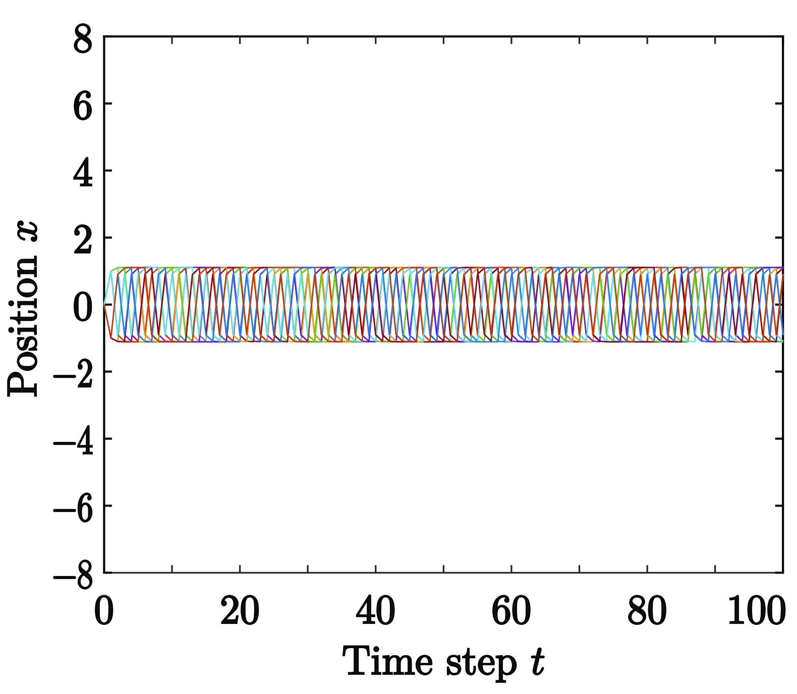
(a) $\alpha=0.1$.

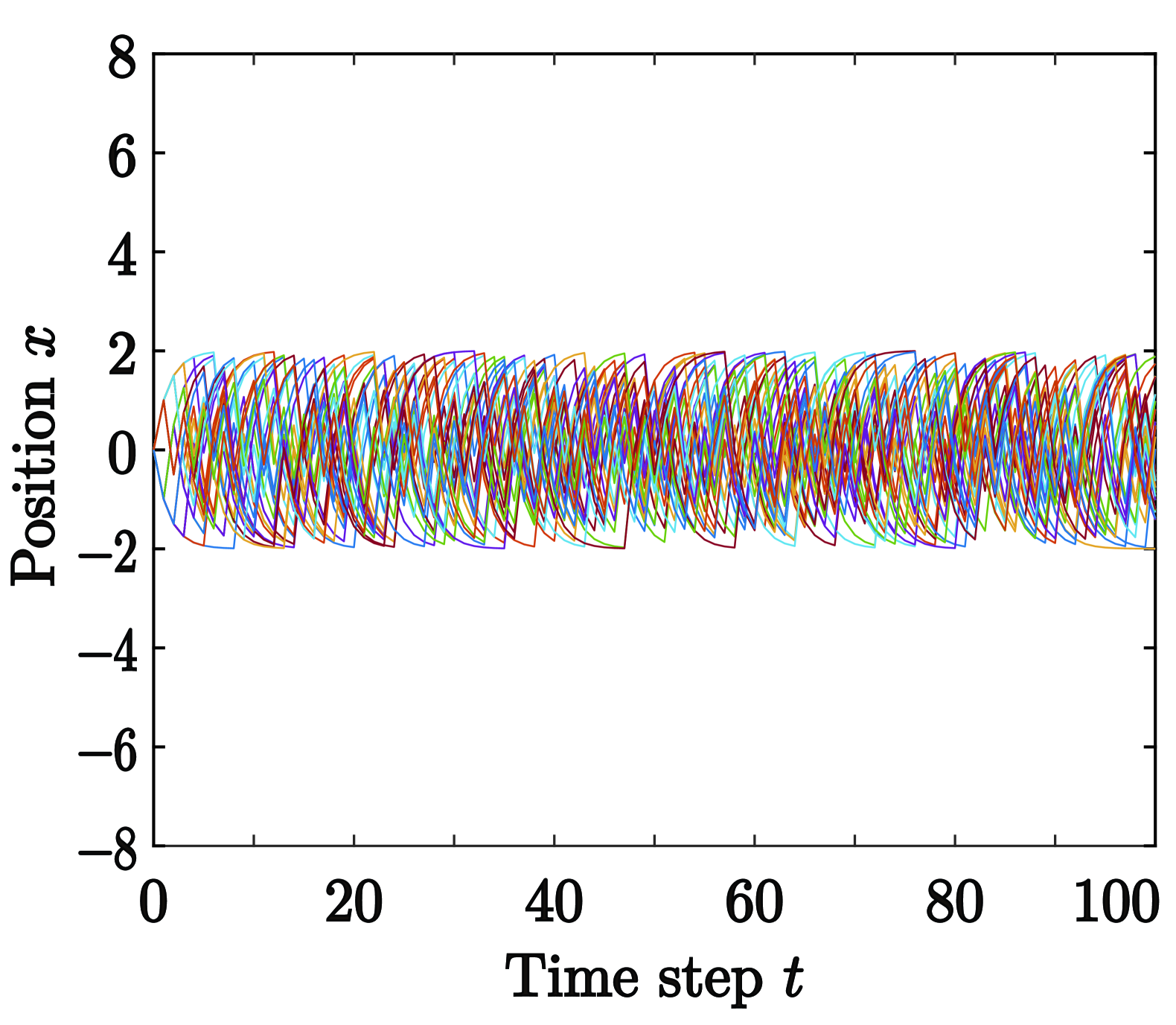
(b) $\alpha=0.5$.

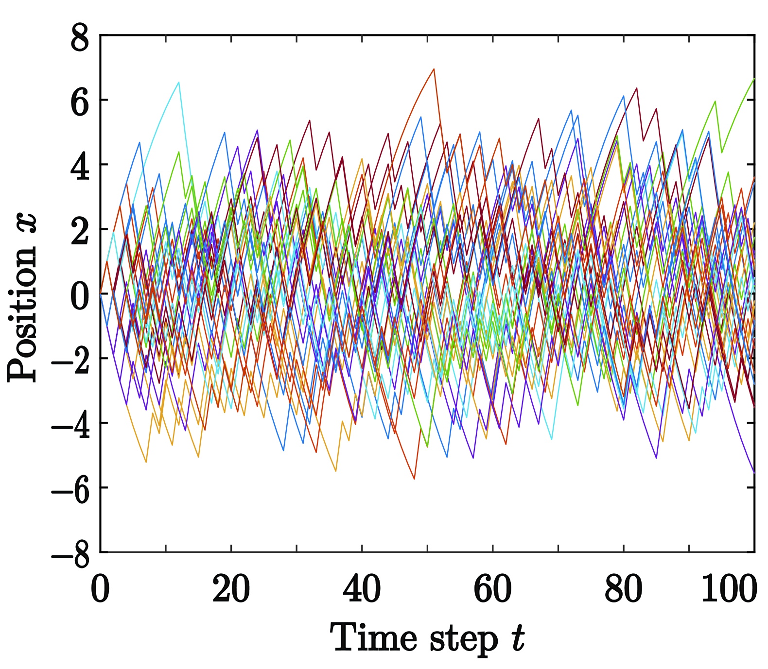
(c) $\alpha=0.9$.

Figure 1: Path trajectories of ARWers from time step $t=0$ to $t=100$ in the cases that parameter $\alpha$ is (a) $0.1$, (b) $0.5$, and (c) $0.9$, respectively. In each case, probability $p$ (see Eq. (2.1)) and the number of trajectories are set to $1/2$ and $30$, respectively. The random variable $X_{t}$ on the positions of ARWers is given in Eq. (2.2).

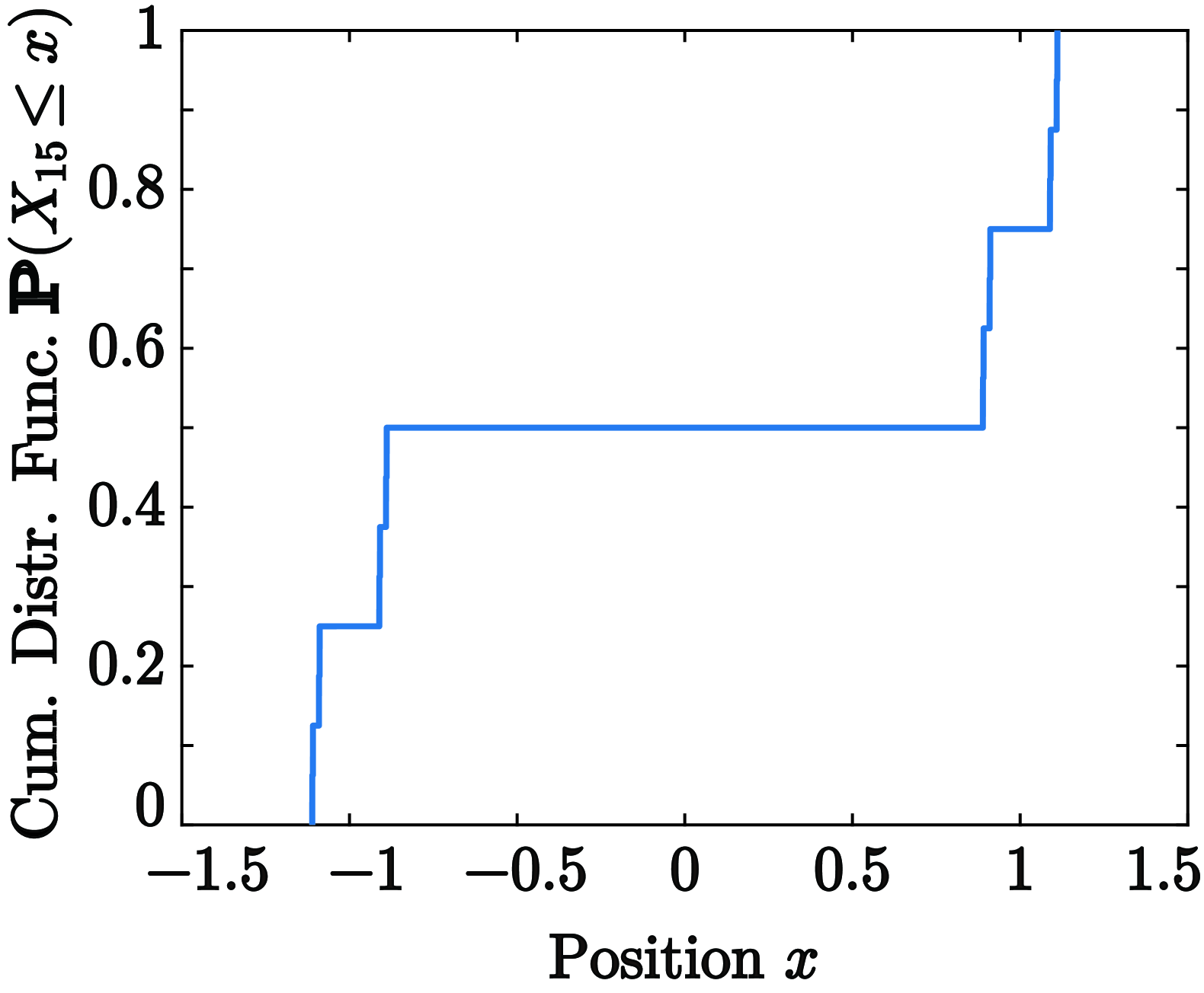
(a) $\alpha=0.1$.

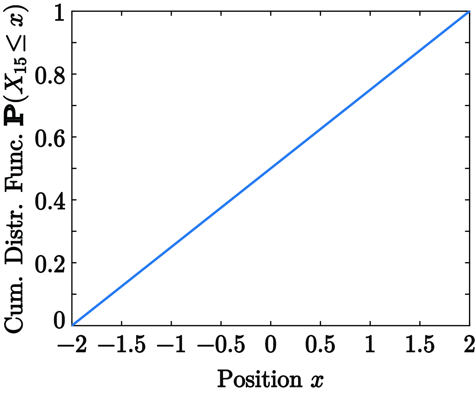
(b) $\alpha=0.5$.

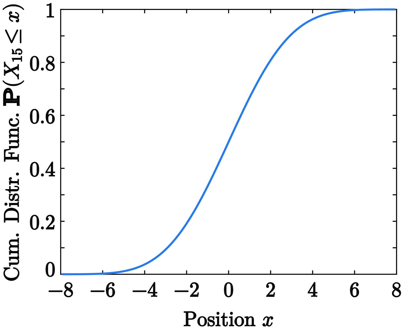
(c) $\alpha=0.9$.

Figure 2: Cumulative distribution functions of the ARWs at time step $t=15$ in the cases that parameter $\alpha$ is (a) $0.1$, (b) $0.5$, and (c) $0.9$, respectively. In each case, probability $p$ (see Eq. (2.1)) is set to $1/2$. The random variable $X_{t}$ on the positions of ARWers is given in Eq. (2.2).

2.2 Inverse path and reachability

In this subsection, we define the notions inverse path and reachability for the proof described later.

Assuming that the final time step of the walks is fixed to $T\in\mathbb{N}$, we define a new sequence $\mbox{\boldmath$\zeta$}^{(T)}=(\zeta^{(T)}_{t})_{t=1}^{T}$ as

$$\zeta^{(T)}_{t}=\xi_{T+1-t}.$$ (2.7)

Then, it is obvious that $\zeta^{(T)}_{t}$ has a one-by-one correspondence with $\xi_{t}$ and is probabilistically determined by the rule same as Eq. (2.1). We set another sequence $(Y^{(T)}_{t})_{t=0}^{T}$ defined by

$$Y^{(T)}_{0}=0,\quad Y^{(T)}_{t}=Y^{(T)}_{t-1}+\alpha^{t-1}\zeta^{(T)}_{t}=\sum_{s=1}^{t}\alpha^{s-1}\zeta^{(T)}_{s}\quad(t\geq 1),$$ (2.8)

as the inverse path of $(X_{t})_{t=0}^{T}$. It is clear that

$$Y^{(T)}_{T}=X_{T}.$$ (2.9)

Eq. (2.9) ensures that we can use $Y_{T}^{(T)}$ instead of $X_{T}$ in the discussion of probability distributions. However, we should note that the sequence $(X_{t})_{t=0}^{T}$ is generally different from $(Y_{t}^{(T)})_{t=0}^{T}$.

Next, we define the reachability. For the walker of the antlion random walk, a position $x\in\mathbb{R}$ is reachable when for all $\epsilon>0$, there exists time $t\in\mathbb{N}\setminus\{0\}$ which satisfies

$$\mathbb{P}(|X_{t}-x|<\epsilon)>0.$$ (2.10)

3 Results

This section is devoted to our main results.

3.1 Characteristic values

By direct calculations, we have some characteristic values, such as expected value, variance, and the upper and lower bounds of $X_{t}$ as follows:

Proposition 3.1.

For $t\geq 1$, the expected value and the variance of $X_{t}$ are

$$\operatorname{\mathbb{E}}[X_{t}] =(1-2p)\sum_{s=1}^{t}\alpha^{s-1},$$ (3.1)

$$\operatorname{\mathbb{V}}[X_{t}] =4p(1-p)\sum_{s=1}^{t}\alpha^{2(s-1)}.$$ (3.2)

For $t\geq 0$, there exist the upper and lower bounds of $X_{t}$ and they are given by

$$\operatorname{sup}X_{t}=\displaystyle\frac{\,1\,}{\,1-\alpha\,},\quad\operatorname{inf}X_{t}=-\displaystyle\frac{\,1\,}{\,1-\alpha\,},$$ (3.3)

respectively.

• First, we prove expected value and variance by induction. For $t=1$, $\mathbb{P}(X_{1}=-1)=p$ and $\mathbb{P}(X_{1}=+1)=1-p$ hold, and thus we have

  $$\operatorname{\mathbb{E}}[X_{1}] =(-1)\cdot p+(+1)\cdot(1-p)=1-2p,$$ (3.4)

  $$\operatorname{\mathbb{V}}[X_{1}] =(-1-1+2p)^{2}\cdot p+(1-1+2p)^{2}\cdot(1-p)=4p(1-p).$$ (3.5)

  Assume that Eqs. (3.1) and (3.2) hold for a certain $t$. Then $\operatorname{\mathbb{E}}[X_{t+1}]$ and $\operatorname{\mathbb{V}}[X_{t+1}]$ can be calculated as

  $$\begin{split}\operatorname{\mathbb{E}}[X_{t+1}]&=\operatorname{\mathbb{E}}[\alpha X_{t}+\xi_{t}]=\alpha\operatorname{\mathbb{E}}[X_{t}]+\operatorname{\mathbb{E}}[\xi_{t}]\\ &=\alpha(1-2p)\sum_{s=1}^{t}\alpha^{s-1}+1-2p=(1-2p)\sum_{s=1}^{t+1}\alpha^{s-1},\end{split}$$ (3.6)

  $$\begin{split}\operatorname{\mathbb{V}}[X_{t+1}]&=\operatorname{\mathbb{V}}[\alpha X_{t}+\xi_{t}]=\alpha^{2}\operatorname{\mathbb{V}}[X_{t}]+\operatorname{\mathbb{V}}[\xi_{t}]\\ &=4\alpha^{2}p(1-p)\sum_{s=1}^{t}\alpha^{2(s-1)}+4p(1-p)=4p(1-p)\sum_{s=1}^{t+1}\alpha^{2(s-1)}.\end{split}$$ (3.7)

  Note that $\xi_{1}=X_{1}$ and $\xi_{t}$-s are i.i.d.

  Next, we consider the upper and lower bounds. Since $0<\alpha<1$, we have

  $$X_{t}=\sum_{s=1}^{t}\alpha^{t-s}\xi_{s}\leq\sum_{s=1}^{t}\alpha^{t-s}=\displaystyle\frac{\,1-\alpha^{t}\,}{\,1-\alpha\,}<\lim_{t\to\infty}\displaystyle\frac{\,1-\alpha^{t}\,}{\,1-\alpha\,}=\displaystyle\frac{\,1\,}{\,1-\alpha\,},$$ (3.8)

  for all time $t$. On the other hand, for all $\epsilon>0$, let $T\in\mathbb{N}$ be an integer which satisfies $\alpha^{T}<(1-\alpha)\epsilon$. Then we obtain

  $$X_{T}\leq\sum_{s=1}^{T}\alpha^{T-s}=\displaystyle\frac{\,1-\alpha^{T}\,}{\,1-\alpha\,},$$

  equality holds when $\xi_{s}=1\;(s=1,\,\cdots,\,T)$. Thus for all $\epsilon>0$, there exists $T\in\mathbb{N}$ which satisfies

  $$\mathbb{P}\left(\left|X_{T}-\displaystyle\frac{\,1\,}{\,1-\alpha\,}\right|<\epsilon\right)>0.$$ (3.9)

  By Eqs. (3.8) and (3.9), we conclude that the upper bound $\operatorname{sup}X=\displaystyle\frac{\,1\,}{\,1-\alpha\,}$.

  In the same manner, the lower bound of $X_{t}$ is obtained as follows:

  $$X_{t}=\sum_{s=1}^{t}\alpha^{t-s}\xi_{s}\geq-\sum_{s=1}^{t}\alpha^{t-s}=-\displaystyle\frac{\,1-\alpha^{t}\,}{\,1-\alpha\,}>\lim_{t\to\infty}-\displaystyle\frac{\,1-\alpha^{t}\,}{\,1-\alpha\,}=-\displaystyle\frac{\,1\,}{\,1-\alpha\,},$$ (3.10)

  and there exists $T\in\mathbb{N}$ which satisfies

  $$\mathbb{P}\left(\left|X_{T}-\left(-\displaystyle\frac{\,1\,}{\,1-\alpha\,}\right)\right|<\epsilon\right)>0.$$ (3.11)

  Therefore, we have the lower bound $\operatorname{inf}X_{t}=-1/(1-\alpha)$.         

It should be noted that the results in the case of $\alpha=1$ are identical to those of simple RWs:

$$\operatorname{\mathbb{E}}[X_{t}]=t(1-2p),\ \operatorname{\mathbb{V}}[X_{t}]=4tp(1-p).$$

Next, we consider the positive-side residence time $T_{+}(t)$ defined as follows:

$$T_{+}(t)=\left|\{s=1,\,\cdots,\,t\ |\ X_{s}\geq 0\}\right|.$$

As stated by the following proposition, the behavior of the positive-side residence time of the ARW is significantly different from that of the simple RW, where we can observe the arcsine law[Lévy1940], making it highly interesting.

Proposition 3.2.

For $0<\alpha\leq 1/2$, at time $t$, the positive-side residence time of the ARW $T_{+}(t)$ follows a binomial distribution $B(t,1-p)$. Additionally, for $1/2<\alpha<1$, if $t$ satisfies $\alpha^{t}-2\alpha+1>0$, the positive-side residence time of the ARW $T_{+}(t)$ also follows a binomial distribution $B(t,1-p)$.

• For $0<\alpha\leq 1/2$, we have the following relation:

  $$|\alpha X_{t-1}|\leq\sum_{k=1}^{t-1}\alpha^{k}=\alpha\frac{1-\alpha^{t-1}}{1-\alpha}<\frac{\alpha}{1-\alpha}<1,$$ (3.12)

  which leads to the inequality $-1+\alpha X_{t-1}<0$. Note that the inequality in the far right-hand side of Eq. (3.12) is derived from the fact that $\alpha<1/2$ implies $\alpha<1/2<1-\alpha$. Then $X_{t}>0$ gives $\xi_{t}=1$ and the positive-side residence time is equal to the number of $\xi_{s}$ satisfying $\xi_{s}=1$ among $(\xi_{s})_{s=1}^{t}$. Since $\mathbb{P}(\xi_{s}=1)=1-p$, we conclude that the positive-side residence time of the ARW follows a binomial distribution $B(t,\,1-p)$.

  Next, we consider the case $1/2<\alpha<1$ and $\alpha^{t}-2\alpha+1>0$. For any time $t$, we have

  $$X_{t} \geq\xi_{t}-\sum_{s=1}^{t-1}\alpha^{t-s}=\xi_{t}-\frac{\alpha-\alpha^{t}}{1-\alpha}$$

  $$=\begin{cases}\displaystyle\frac{\,1-2\alpha+\alpha^{t}\,}{\,1-\alpha\,}\vrule height=0.0pt,width=0.0pt,depth=15.0pt\quad&(\xi_{t}=1),\\ \displaystyle\frac{\,-1+\alpha^{t}\,}{\,1-\alpha\,}\quad&(\xi_{t}=-1).\end{cases}$$

  Then, if $t$ satisfies $\alpha^{t}-2\alpha+1>0$ and $\xi_{t}=1$, we get $X_{t}>0$. In the same manner, if $t$ satisfies $\alpha^{t}-2\alpha+1>0$ and $\xi_{t}=-1$, we obtain $X_{t}<0$. Thus, since the sign of $\xi_{t}$ matches the sign of $X_{t}$, the positive-side residence time of the ARW follows the binomial distribution $B(t,\,1-p)$.         

3.2 Phase transition

This subsection deals with the phase transition of the ARW.

Theorem 3.3.

For $0<\alpha<1/2$, there exists a position $r\in[-1/(1-\alpha),\,1/(1-\alpha)]$, which is not reachable for the walker of ARW. On the other hand, for $1/2\leq\alpha<1$, any position $r\in[-1/(1-\alpha),\,1/(1-\alpha)]$ is reachable for the walker of ARW.

• When $0<\alpha<1/2$, let $r$ and $\epsilon$ be

  $$r=\epsilon=\frac{1-2\alpha}{2(1-\alpha)}>0.$$

  For the inequality $|X_{t}-r|<\epsilon$ to hold at time $t$, it is necessary to satisfy $X_{t}>0$. In that case, we have $\xi_{t}=1$, as we discussed in Proposition 3.2, and the following inequality is obtained:

  $$X_{t}=1+\alpha X_{t-1}>1-\frac{\alpha}{1-\alpha}=\frac{1-2\alpha}{1-\alpha}>0.$$

  Thus for all time $t$, we have

  $$X_{t}-r>\frac{1-2\alpha}{1-\alpha}-\frac{1-2\alpha}{2(1-\alpha)}=\frac{1-2\alpha}{2(1-\alpha)},$$

  which results in

  $$\mathbb{P}(|X_{t}-r|<\epsilon)=0,$$

  indicating that $r$ is not reachable.

  Next, we consider $\alpha=1/2$. It immediately follows from the definition that any $r$ for which there exists $t$ such that $X_{t}=r$ is reachable. Therefore, we consider $r$ that does not satisfy this condition. When $\alpha=1/2$, we have the following equation at time $t$:

  $$X_{t}+\sum_{s=1}^{t}\left(\displaystyle\frac{\,1\,}{\,2\,}\right)^{t-s}=\sum_{\{s:\xi_{s}=1\}}1\cdot\left(\displaystyle\frac{\,1\,}{\,2\,}\right)^{t-s-1}+\sum_{\{s:\xi_{s}=-1\}}0\cdot\left(\displaystyle\frac{\,1\,}{\,2\,}\right)^{t-s-1}.$$ (3.13)

  The right-hand side of Eq. (3.13) represents the entire set of binary numbers with 2 digits in the integer part and $(t-2)$ digits in the fractional part, ranging from 0 to less than 4, corresponding to the entire set of sequences $\{\xi_{s}\}_{s=1}^{t}$. Thus, $X_{t}$ represents the entire set of binary numbers with $(t-1)$ digits in the fractional part, greater than $-2$ and less than 2, corresponding to the entire set of sequences $\{\xi_{s}\}_{s=1}^{t}$. Therefore, for any $\epsilon>0$, if we consider a time $T$ such that $(1/2)^{T}<\epsilon$, it holds that for any $r\in[-2,2]$, $\mathbb{P}(|X_{T}-r|<\epsilon)>0$ is satisfied. In other words, any point $r\in[-2,2]$ is reachable.

  Finally, we discuss $1/2<\alpha<1$. As in the case of $\alpha=1/2$, we exclude and consider separately the case where there exists a time $t$ such that $X_{t}=r$. It suffices to consider $r>0$, as the case $r<0$ can be proven by applying the argument for $r>0$ multiplied by $-1$. First, take a sufficiently large natural number $T$ for $\epsilon>0$, the conditions specified later. Then, there exists $t_{1}$ such that $\zeta_{1}=\zeta_{2}=\dots=\zeta_{t_{1}}=1$ and $Y_{t_{1}-1}^{(T)}<r<Y_{t_{1}}^{(T)}$, where $\zeta_{1}=\xi_{T},\,\zeta_{2}=\xi_{T-1},\,\dots\,,\,\zeta_{k}=\xi_{T+1-k},\,\dots,\,\zeta_{T}=\xi_{1}$. In other words, reinterpret $\xi$ and $\zeta$ so that $Y_{t}^{(T)}=Y_{t-1}^{(T)}+\alpha^{t}\zeta_{t}$. If $Y_{t_{1}}^{(T)}$ satisfies $|Y_{t_{1}}^{(T)}-r|<\alpha^{t_{1}}<\epsilon$, we have $T=t_{1}$. Otherwise, $|Y_{t_{1}}^{(T)}-r|\geq\epsilon$, there exists $t_{2}$ such that $Y_{t_{2}}<r<Y_{t_{2}-1}$ and $\zeta_{t_{1}+1}=\dots=\zeta_{t_{2}}=-1$. This is because $\alpha^{t_{1}}<\alpha^{t_{1}+1}/(1-\alpha)$ and the following inequality:

  $$Y_{t_{1}}^{(T)}-\sum_{k=t_{1}+1}^{\infty}\alpha^{k}=Y_{t_{1}}^{(T)}-\displaystyle\frac{\,\alpha^{t_{1}+1}\,}{\,1-\alpha\,}<Y_{t_{1}-1}^{(T)}<r.$$

  If $|Y_{t_{2}}^{(T)}-r|<\alpha^{t_{2}}<\epsilon$, we get $T=t_{2}$. As can be seen so far, $T$ satisfies the following conditions: $\alpha^{T}<\epsilon$, $|Y_{T}^{(T)}-r|<\epsilon$, and either $Y_{T-1}^{(T)}<r<Y_{T}^{(T)}$ or $Y_{T}^{(T)}<r<Y_{T-1}^{(T)}$. Using the same argument as for $t_{1},t_{2}$, we obtain the sequence $t_{1},t_{2},\dots,T$. Here, $Y_{t_{2j-1}-1}^{(T)}<r<Y_{t_{2j-1}}^{(T)}$ and $Y_{t_{2j}}^{(T)}<r<Y_{t_{2j}-1}^{(T)}$, with $j=1,2,\dots$. Since $Y^{(T)}_{T}=X_{T}$, we have

  $$\mathbb{P}(|Y_{T}^{(T)}-r|<\epsilon)=\mathbb{P}(|X_{T}-r|<\epsilon)\geq\displaystyle\frac{\,1\,}{\,2^{T}\,}>0.$$ (3.14)

  Since Eq. (3.14) means that the position $r$ is reachable, the proof is completed.         

It should be noted that the case of $\alpha=1/2$ is identical to the one discussed in Ref. [18].

3.3 Distance from the normal distribution

In this subsection, we examine the probability distribution of the symmetric ARW with $p=1/2$ and present numerical results on its differences from the normal distribution.

3.3.1 Probability distribution

First, we describe one of the properties of the ARW for $\alpha\in\mathbb{Q}$.

Proposition 3.4.

Let $\alpha\in\mathbb{Q}$. For any $x\in\mathbb{R}$ such that $X_{t}=x$ at a given time $t$, the path of the ARW to $x$ is unique.

• We demonstrate this proposition using proof by contradiction. Suppose that at a certain time $t$, there exist two distinct sequences $\{\xi_{s}\}_{s=1}^{t}$ and $\{\xi^{{}^{\prime}}_{s}\}_{s=1}^{t}$ such that

  $$\sum_{s=1}^{t}\alpha^{t-s}\xi_{s}=\sum_{s=1}^{t}\alpha^{t-s}\xi^{{}^{\prime}}_{s}.$$ (3.15)

  Here, each term $\xi_{s}$ and $\xi^{{}^{\prime}}_{s}$ is either $1$ or $-1$. Since $\alpha$ is a rational number, it can be expressed as $\alpha=m/n$ using two coprime natural numbers $m$ and $n$. Thus, Eq. (3.15) can be transformed into the following equation.

  $$\sum_{s=1}^{t}\left(\displaystyle\frac{\,m\,}{\,n\,}\right)^{t-s}\xi_{s}=\sum_{s=1}^{t}\left(\displaystyle\frac{\,m\,}{\,n\,}\right)^{t-s}\xi^{{}^{\prime}}_{s}$$

  $$\sum_{s=1}^{t}m^{t-s}n^{s-1}\xi_{s}=\sum_{s=1}^{t}m^{t-s}n^{s-1}\xi^{{}^{\prime}}_{s}$$

  $$\sum_{s=1}^{t}m^{t-s}\left(\displaystyle\frac{\,\xi_{s}-\xi^{{}^{\prime}}_{s}\,}{\,2\,}\right)n^{s-1}=0.$$ (3.16)

  Note the following:

  $$\frac{\xi_{s}-\xi^{{}^{\prime}}_{s}}{2}=\begin{cases}1&(\xi_{s}=1\text{ and }\xi^{{}^{\prime}}_{s}=-1),\\ -1&(\xi_{s}=-1\text{ and }\xi^{{}^{\prime}}_{s}=1),\\ 0&(\text{otherwise}).\end{cases}$$ (3.17)

  Since $m$ and $n$ are coprime, each term in Eq. (3.16) equals 0, which contradicts the assumption that the sequences $\{\xi_{s}\}_{s=1}^{t}$ and $\{\xi^{{}^{\prime}}_{s}\}_{s=1}^{t}$ are distinct. Thus, the proposition is proven.         

On the other hand, when $\alpha$ is an irrational number, there exist cases, such as $\alpha=(-1+\sqrt{5})/2$, where the path to a point $x$ is not unique. The following corollary is immediately obtained by Proposition 3.4.

Corollary 3.5.

Let $\alpha\in\mathbb{Q}$. For any point $x\in\mathbb{R}$, the probability distribution of the symmetric ARW at time $t$ is given by:

$$\mathbb{P}(X_{t}=x)=\begin{cases}2^{-t},&(x\text{ is reachable at time }t),\\ 0,&(\text{otherwise}).\end{cases}$$

Corollary 3.5 indicates that the symmetric ARW is uniformly distributed over the points where it exists at the given time. However, except for the case $\alpha=1/2$, these points are not uniformly present within the interval $[-1/(1-\alpha),1/(1-\alpha)]$.

3.3.2 Similarity to the normal distribution

As described so far, the probability distribution of the symmetric ARW differs significantly from that of a simple RW. Yet, by focusing on their cumulative distribution functions and comparing the two, we discover not only their differences but also their similarities. As seen in Fig. 2, the cumulative distribution function of the ARW with $\alpha=0.9$ has a shape similar to that of the normal distribution, which is the limiting distribution of the simple RW. This observation of qualitatively justified by laying the two cumulative distribution functions as shown in Fig.  3(3). The figure also indicates that, at least at time step $t=15$, the cumulative distribution function of ARWs is rather closer to that of the normal distribution than that of the simple RWs. In this subsection, to quantitatively represent this property, we calculate their distances from the normal distribution using the Cramér–von Mises (CvM) distance [19, 20].

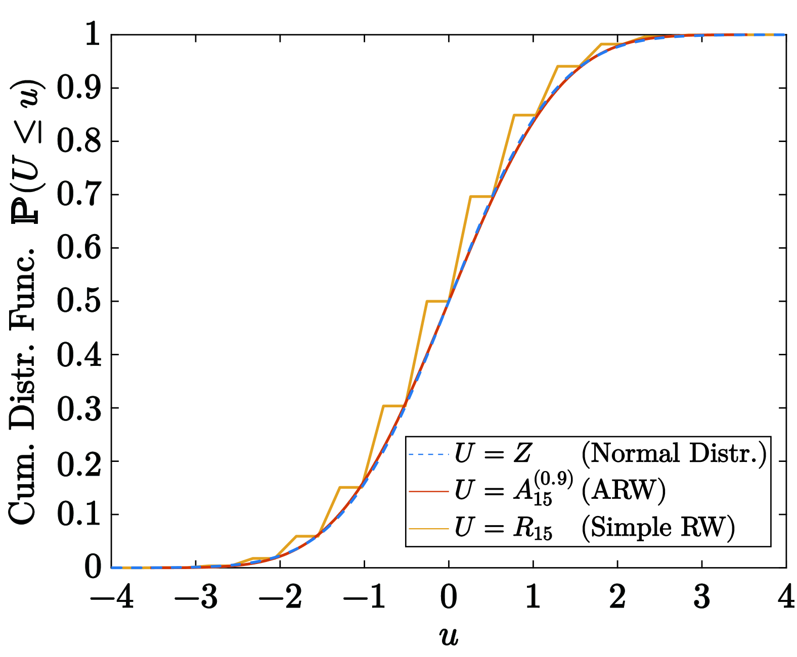
(a) Comparison of the cumulative distribution functions among the standard normal distribution, the ARW, and the simple RW with time step $t=15$.

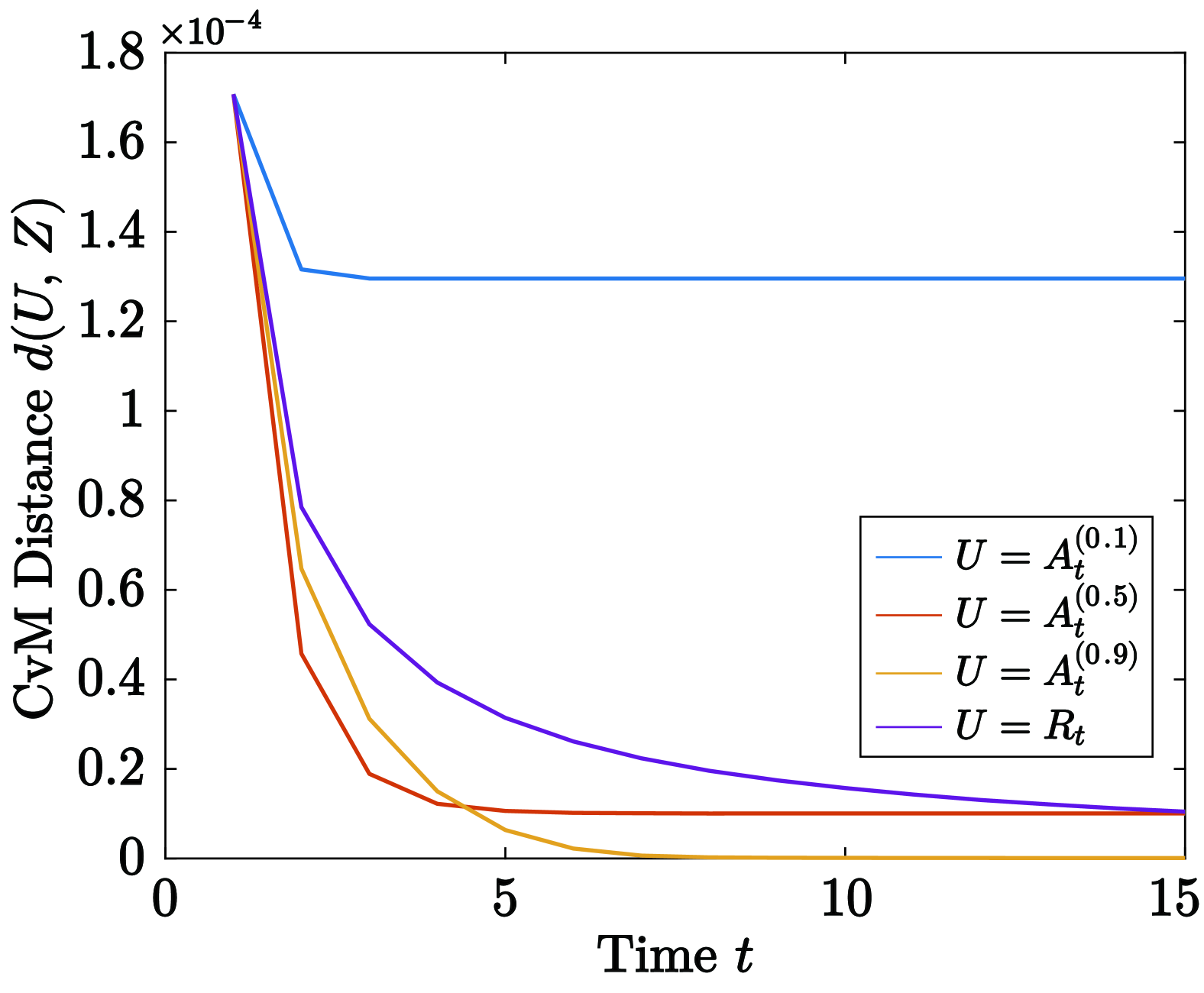
(b) Calculational results for the CvM distance with the standard normal distribution over time step $t$ with $t=1,\,\cdots,\,15$ in the cases of $\alpha=0.1$, $0.5$, and $0.9$, and simple RWs.

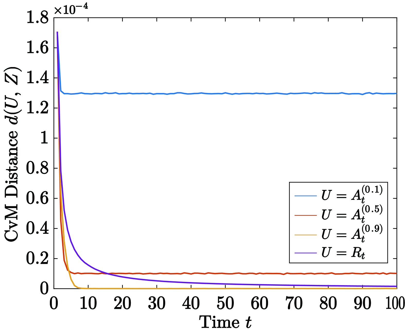
(c) Simulational results for the CvM distance with the standard normal distribution over time step $t$ with $t=1,\,\cdots,\,100$ in the cases of $\alpha=0.1$, $0.5$, and $0.9$, and simple RWs.

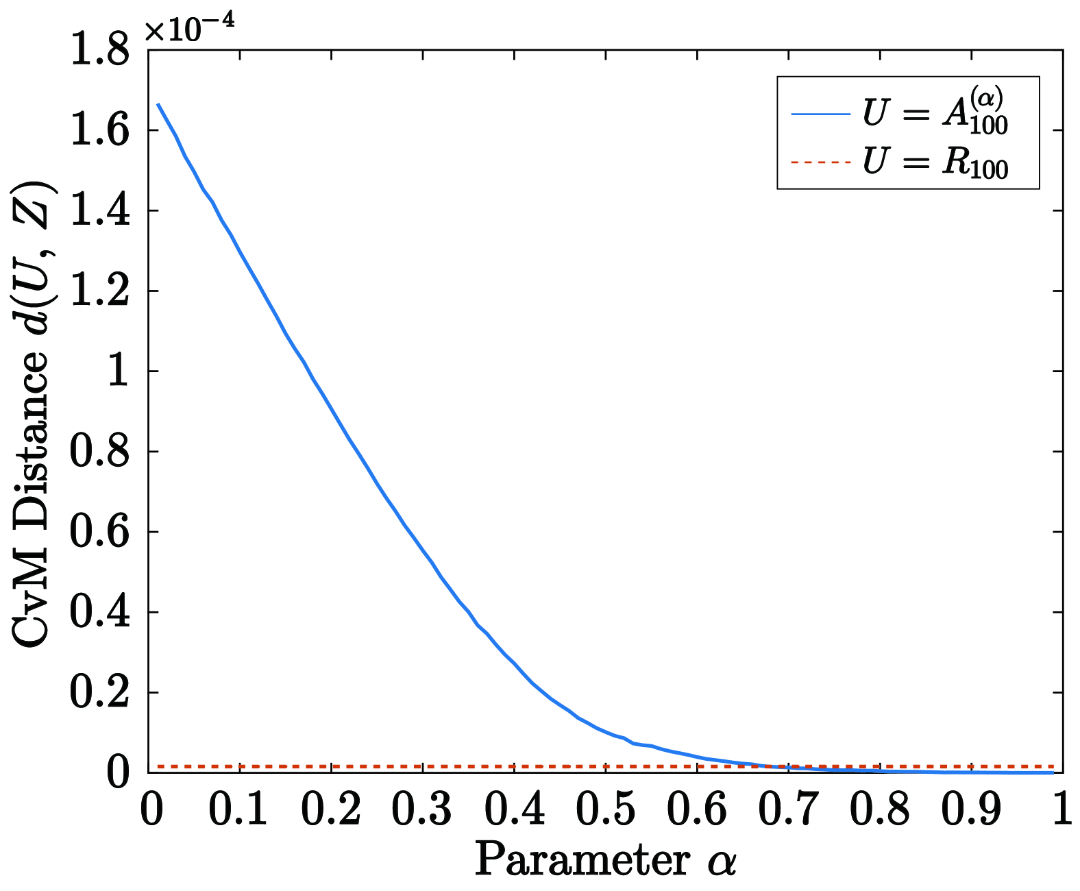
(d) Simulational results for the CvM distance between the normalized random variable of the ARW at time step $t=100$ and the standard normal distribution over the parameter $\alpha$ with $\alpha=0.01,\,0.02,\,\cdots,\,0.99$.

Figure 3: Comparision of the standardized random variables among the normal distribution, the ARWs, and the simple RWs. The random variables at time step $t$ are denoted by $Z$, $A_{t}^{(\alpha)}$, and $R_{t}$, respectively. Subfigures (3) and (3), displaying numerical results, drive 50,000 walkers for each walk. The definition of (asymptotic) CvM distance $d(U,\,Z)$ can be found in Eq. (3.21).

The CvM distance is used to evaluate the similarity between two probability distributions and is applied in various fields, including statistical hypothesis testing and the evaluation of generative models in machine learning [21, 22]. We should note that the smaller this value, the greater the similarity between the two distributions. From now on, we examine the dissimilarity between the cumulative distribution function of the normal distribution and those of the ARW and the simple RW.

Let $S_{t}$ be the random variable representing the position of a symmetric simple RW at time $t$, and let $Z$ be a random variable following the standard normal distribution. In this section, we calculate the cumulative distribution functions of the standardized random variable $A_{t}^{(\alpha)}:=\sqrt{(1-\alpha)/(1-\alpha^{2t})}X_{t}$, which is associated with the ARW, and the random variable $R_{t}:=S_{t}/\sqrt{t}$, which is associated with the simple RW.

In the following, we calculate the CvM distances between $A_{t}^{(\alpha)}$ or $R_{t}$ and the standard normal variable $Z$. The CvM distance $D(U,\,V)$ between random variables $U$ and $V$ is given by

$$D(U,\,V)=\int_{-\infty}^{\infty}\left\{\mathbb{P}(U\leq u)-\mathbb{P}(V\leq u)\right\}^{2}{\rm d}u.$$ (3.18)

Here by the definition of integration, $D(U,\,V)$ can be rewritten as

$$D(U,\,V)=\lim_{m_{1}\to-\infty}\lim_{m_{2}\to\infty}\lim_{n\to\infty}d(U,\,V;\,m_{1},\,m_{2},\,n),$$ (3.19)

where

$$d(U,\,V;\,m_{1},\,m_{2},\,n)=\displaystyle\frac{\,m_{2}-m_{1}\,}{\,n\,}\sum_{k=1}^{n}\left\{\mathbb{P}\left(U\leq m_{1}+\displaystyle\frac{\,m_{2}-m_{1}\,}{\,n\,}k\right)-\mathbb{P}\left(V\leq m_{1}+\displaystyle\frac{\,m_{2}-m_{1}\,}{\,n\,}k\right)\right\}^{2}$$ (3.20)

with $m_{1}<m_{2}$ and $n\in\mathbb{N}$. It should be noted that $m_{1}$ and $m_{2}$ represent the left and right edges of the interval, respectively, and $n$ denotes the number of division in the interval $[m_{1},\,m_{2}]$. In this paper, the CvM distance is asymptotically calculated as $d(U,\,V;\,m_{1},\,m_{2},\,n)$ with sufficiently wide range $[m_{1},\,m_{2}]$ and large $n$. Specifically, we set $(m_{1},\,m_{2},\,n)=(-3,\,3,\,600)$; that is, the (asymptotic) CvM distances are defined as follows:

$$d(U_{t},\,Z)=d(U_{t},\,Z;\,-3,\,3,\,600)=\displaystyle\frac{\,1\,}{\,100\,}\sum_{k=1}^{600}\left\{\mathbb{P}\left(U_{t}\leq-3+\displaystyle\frac{\,k\,}{\,100\,}\right)-\mathbb{P}\left(Z\leq-3+\displaystyle\frac{\,k\,}{\,100\,}\right)\right\}^{2},$$ (3.21)

where $U_{t}=A_{t}^{(\alpha)}$, $R_{t}$.

Figure 3(3) presents the numerical calculations of the CVM distances between the cumulative distribution functions of the normal distribution and those of the ARW with $\alpha=0.1$, $0.5$, $0.9$ and the simple RW over the time interval from 1 to 15. We can see that at early stage, the ARWs with $\alpha=0.5$ or $0.9$ have a cumulative distribution functions closer than that of the simple RWs. It is difficult for computers to obtain similar results until too large time step $t$ as calculational results, in particular for ARWs, but is possible by observing the behavior of a lot of virtual walkers driven by the random numbers as shown in Fig. 3(3). This figure clarifies that the actual CvM distances can converge to some values, which is not $0$, while the one with the simple RWs seems to converge to $0$ for sufficiently large $t$. Figure 3(3) shows $\alpha$-dependency of the CvM distance $d(A_{100}^{(\alpha)},\,Z)$ between the cumulative distribution functions of ARWs and the normal distribution at time $t=100$, which appears to be almost identical to the convergent value of $d(A_{t}^{(\alpha)},\,Z)$, judging from Fig. 3(3). We can see that the value is monotonically decreasing for $\alpha$. The orange dotted line in this figure indicates the CvM distance $d(R_{100},\,Z)$ between the simple-RW distribution and the standard normal distribution. In our results, if $\alpha$ is greater than $0.68$, the CvM distance gets closer than that of the simple RWs at time $t=100$.

Based on these results, the cumulative distribution function of the ARW is considered to have the following characteristics: first, the cumulative function of the ARWs converge to some distributions much faster than that of the simple RWs. Next, for the value of $\alpha$ larger than a certain size, at least $\alpha>0.5$ as shown in Fig. 3(3), the distributions of ARWs are much closer to that of the normal distribution than that of the simple RWs at the early stage. The characteristic observed here is expected to be related to the acceleration of decision-making processes.

Furthermore, at time $t=100$, the CvM distance from the normal distribution has largely stabilized for the ARW, whereas it continues to decrease for the RW. This suggests that while the distribution of the RW converges to the normal distribution in a mathematically rigorous sense, the ARW does not. In fact, the following theorem holds.

Theorem 3.6.

For any $\alpha\in(0,\,1)$, the random variable $A_{t}^{(\alpha)}$ does not weakly converge to $Z$.

• Since $X_{t}\geq-\displaystyle\frac{\,1-\alpha^{t}\,}{\,1-\alpha\,}$ and $\displaystyle\frac{\,1-\alpha^{t}\,}{\,1-\alpha^{2t}\,}<1$, we have

  $$A_{t}^{(\alpha)}=\sqrt{\frac{1-\alpha}{1-\alpha^{2t}}}X_{t} \geq-\sqrt{\frac{1-\alpha}{1-\alpha^{2t}}}\displaystyle\frac{\,1-\alpha^{t}\,}{\,1-\alpha\,}=-\sqrt{\frac{1-\alpha^{t}}{1-\alpha^{2t}}}\sqrt{\frac{1-\alpha^{t}}{1-\alpha}}$$

  $$>-\sqrt{\frac{1-\alpha^{t}}{1-\alpha}}>-\displaystyle\frac{\,1\,}{\,\sqrt{1-\alpha}\,},$$

  for all time $t$. Then, we obtain

  $$\mathbb{P}\left(A_{t}^{(\alpha)}<-\displaystyle\frac{\,1\,}{\,\sqrt{1-\alpha}\,}\right)=0.$$ (3.22)

  By Eq. (3.22) and the fact that $\mathbb{P}\left(Z<-\frac{1}{\sqrt{1-\alpha}}\right)>0$, $A_{t}^{(\alpha)}$ does not weakly converge to $Z$ for any $\alpha$.         

By the definition of weak convergence, note that if a random variable $U$ depending on time $t$ weakly converges to $Z$, then $D(U,\,Z)$ must converge to $0$.

4 Conclusion and Discussion

In this study, we analyzed a random walk (ARW) in which the walker is drawn toward the origin. We calculated various characteristics, including the expected value, variance, upper and lower bounds, and positive-side residence time. In addition, we discussed the phase transition in the behavior of the random walker. Furthermore, the parameter $\alpha$, which characterizes the strength of the tendency for the walker to be drawn toward the origin and is referred to as the forgetting parameter in the previous study, was proven to exhibit distinct probabilistic properties when $\alpha$ is a rational number, differing from those of the simple RW. On the other hand, numerical calculations confirmed that, similar to the probability distribution of the simple RW, the probability distribution of the ARW also tends to approach a normal distribution. Moreover, by comparing using the Cramér–von Mises distance, it was observed that at smaller time steps, the ARW converges to the normal distribution even more rapidly by computing the distance between distributions.

As future work, possible directions include an investigation of the positive-side residence time at general time steps for $\alpha>1/2$ and a theoretical analysis of the relationship between the rapid convergence of the ARW to the normal distribution and the acceleration of decision-making. Depending on the value of $\alpha$, the CvM distance is expected to converge to a certain value as time approaches infinity. Determining this limiting value remains an open problem. By considering the exterior of the support of the distribution of the ARW, the following lower bound is obtained.

$$D(A_{t}^{(\alpha)},Z)>2\int_{-\infty}^{-\frac{1}{\sqrt{1-\alpha}}}\left\{\mathbb{P}(Z\leq u)\right\}^{2}{\rm d}u.$$

However, further analysis is required for the interior of the support.

Acknowledgments: A.N. is partially financed by the Grant-in-Aid for Young Scientists of Japan Society for the Promotion of Science (Grant No. JP23K13017). T.Y. is supported by Grant-in-Aid for JSPS Fellows (Grant No. JP23KJ0384). The authors appreciate to Dr. Masato Takei at Yokohama National University for useful comments.

Data availability statement: The data that support the findings of this study are available from the corresponding author upon reasonable request.

References

- [1] G. F. Lawler and V. Limic, Random Walk: A Modern Introduction. Cambridge University Press, 2010.
- [2] D. Chandler, Introduction to Modern Statistical Mechanics. Oxford University Press, 1987.
- [3] B. G. Malkiel, A Random Walk Down Wall Street: The Time-tested Strategy for Successful Investing. W. W. Norton & Company, Inc., 2011.
- [4] G. M. Viswanathan, E. Raposo, and M. Da Luz, “Lévy flights and superdiffusion in the context of biological encounters and random searches,” Physics of Life Reviews, Vol. 5, No. 3, pp. 133–150, 2008.
- [5] J. T. Abbott, J. L. Austerweil, and T. L. Griffiths, “Random walks on semantic networks can resemble optimal foraging,” Psychological Review, Vol. 122, No. 3, pp. 558–569, 2015.
- [6] F. Xia, J. Liu, H. Nie, Y. Fu, L. Wan, and X. Kong, “Random walks: A review of algorithms and applications,” IEEE Transactions on Emerging Topics in Computational Intelligence, Vol. 4, No. 2, pp. 95–107, 2019.
- [7] L. M. Berliner, “Statistics, probability and chaos,” Statistical Science, pp. 69–90, 1992.
- [8] K. Kitayama, M. Notomi, M. Naruse, K. Inoue, S. Kawakami, and A. Uchida, “Novel frontier of photonics for data processing―Photonic accelerator,” APL Photonics, Vol. 4, No. 9, Art. No. 090901, 2019.
- [9] A. Uchida, K. Amano, M. Inoue, K. Hirano, S. Naito, H. Someya, I. Oowada, T. Kurashige, M. Shiki, S. Yoshimori, K. Yoshimura, and P. Davis, “Fast physical random bit generation with chaotic semiconductor lasers,” Nature Photonics, Vol. 2, No. 12, pp. 728–732, 2008.
- [10] A. Argyris, S. Deligiannidis, E. Pikasis, A. Bogris, and D. Syvridis, “Implementation of 140 Gb/s true random bit generator based on a chaotic photonic integrated circuit,” Optics Express, Vol. 18, No. 18, pp. 18763–18768, 2010.
- [11] M. Naruse, Y. Terashima, A. Uchida, and S.-J. Kim, “Ultrafast photonic reinforcement learning based on laser chaos,” Scientific Reports, Vol. 7, No. 1, Art. No. 8772, 2017.
- [12] T. Mihana, Y. Terashima, M. Naruse, S.-J. Kim, and A. Uchida, “Memory effect on adaptive decision making with a chaotic semiconductor laser,” Complexity, Vol. 2018, No. 1, Art. No. 4318127, 2018.
- [13] H. Robbins, “Some aspects of the sequential design of experiments,” Bulletin of the American Mathematical Society, Vol. 58, No. 5, pp. 527–535, 1952.
- [14] R. S. Sutton and A. G. Barto, Reinforcement Learning: An Introduction. MIT press, 2018.
- [15] S.-J. Kim, M. Aono, and E. Nameda, “Efficient decision-making by volume-conserving physical object,” New Journal of Physics, Vol. 17, No. 8, Art. No. 083023, 2015.
- [16] N. Okada, T. Yamagami, N. Chauvet, Y. Ito, M. Hasegawa, and M. Naruse, “Theory of Acceleration of Decision-Making by Correlated Time Sequences,” Complexity, Vol. 2022, Art. No. 5205580, 2022.
- [17] P. Lévy, “Sur certains processus stochastiques homogènes,” Compositio Mathematica, Vol. 7, pp. 283–339, 1940.
- [18] B. Schmuland, “Random Harmonic Series,” The American Mathematical Monthly, Vol. 110, No. 5, pp. 407–416, 2003.
- [19] H. Cramér, “On the composition of elementary errors: Second paper: Statistical applications,” Scandinavian Actuarial Journal, Vol. 11, No. 1, pp. 141–180, 1928.
- [20] R. von Mises, Wahrscheinlichkeitsrechnung und ihre Anwendung in der Statistik und theoretische Physik. Franz Deuticke, 1931.
- [21] M. G. Bellemare, I. Danihelka, W. Dabney, S. Mohamed, B. Lakshminarayanan, S. Hoyer, and R. Munos, “The Cramer Distance as a Solution to Biased Wasserstein Gradients,” arXiv preprint arXiv:1705.10743, 2017.
- [22] A. Lhéritier and N. Bondoux, “A Cramér Distance perspective on Non-crossing Quantile Regression in Distributional Reinforcement Learning,” in The 25th International Conference on Artificial Intelligence and Statistics, Vol. 151, pp. 5774–5789, PMLR, 2022.