Harnessing electron motion for global spin qubit control

Abstract

Silicon spin qubits are promising candidates for building scalable quantum computers due to their nanometre scale features. However, delivering microwave control signals locally to each qubit poses a challenge and instead methods that utilise global control fields have been proposed. These require tuning the frequency of selected qubits into resonance with a global field while detuning the rest to avoid frequency crowding. Common frequency tuning methods, such as electric-field-induced Stark shift, are insufficient to cover the frequency variability across large arrays of qubits. Here, we argue that electron motion, and especially the recently demonstrated high-fidelity shuttling, can be leveraged to enhance frequency tunability. Our conclusions are supported by numerical simulations proving its efficiency on concrete architectures such as a 2$\times$N array of qubits and the recently introduced looped pipeline architecture. Specifically, we show that the use of our schemes enables single-qubit fidelity improvements up to a factor of 100 compared to the state-of-the-art. Finally, we show that our scheme can naturally be extended to perform two-qubit gates globally.

I Introduction

Silicon-based spin qubits are a promising qubit platform due to their small footprint, high control fidelity [1, 2, 3], long coherence times [4], and their compatibility with nanofabrication techniques of the semiconductor industry [5, 6, 7, 8, 9, 10]. For spin qubits to be a viable option for building scalable quantum computers, methods for controlling a large number of qubits – potentially millions to implement error correction – need to be developed. Particularly, when encoding a qubit in the spin of a single electron, a microwave field in resonance with the Zeeman-split levels leads to Rabi oscillations of the spin system. These fields can be applied locally through surface gate electrodes, but such an approach, applied at scale presents formidable challenges for signal delivery. Instead, a global control field can be applied, and selected spins be brought in and out of resonance by means of frequency tuning [11, 12, 13, 14]. Unfortunately, common frequency tuning techniques are unable to fully correct for the spread of qubit frequencies that are typically found in devices due to variations on the local spin-orbit fields [15, 16, 17].

To ameliorate the situation, recent studies have shown that the spin qubit frequency spread can be reduced by wisely choosing the angle of the static magnetic field with respect to the crystallographic axes of the sample [18, 13]. Complementarily, one can tune the qubit frequencies using electric-field-induced Stark shifts but its limited tuning range – one order of magnitude smaller than the typical frequency spread – forces further measures. A partial solution proposed tuning the $g$-factors using electric-field-induced Stark shifts to place the qubits in to a number of distinct-frequency bins, thereby mitigating the effect of frequency crowding. This way the minimum frequency spacing does not decrease with the system size [19, 14]. By sending tones at resonance with each bin, selected qubits can be driven and the desired global single-qubit gates can be performed. Reference [14] extended this scheme and suggested a way to drive not all but a single qubit, via the addition of SWAP gates. However, none of these works allow for the reliable implementation of single-qubit gates on any subset of qubits, without halving the already critical bin spacing.

Here, we propose to solve the challenge of limited frequency tuning range by leveraging electron motion through the spin qubit nanodevice. Namely, we show that one can reduce the number of distinct frequencies in the frequency spectrum by homogenising the electrons $g$-factors via spin shuttling or via exchange-driven two-qubit SWAPs. More specifically, if an electron experiences a collection of $g$-factors at a rate that is sufficiently fast compared to the Rabi frequency and the qubits frequency dispersion, the electron will acquire an effective homogenised $g$-factor equal to the mean of all experienced $g$-factors. While both methods leverage the same simple idea, we find that the shuttling-based homogenisation is more scalable, and can additionally be utilised for the implementation of two-qubit gates. More than a key component for the development of fault-tolerant architectures [20, 21, 22, 23, 24], spin shuttling turns out to be an enabling tool in the quest for homogeneous devices. It is worth mentioning that our idea is reminiscent of the frequency narrowing phenomenon [25]; however, this concept was never used to perform quantum gates. In this work, we concentrate on electron spin qubits in silicon because of their small spin-orbit fields. However, as we shall see later, our work can be extended to strong spin-orbit systems that present large variations in their spin quantisation axes.

The paper is organised as follows. In Section˜II, we introduce our model for the qubits. Thereafter, in Section˜III we abstractly describe the homogenisation principle before giving two methods to physically implement it, capitalising on the exchange coupling or shuttling. Focusing on the more promising shuttling-based protocol, we then explore its performance for two architectures, namely the 2$\times$N [21, 26] and looped pipeline architectures [24] in Section˜IV. Finally, we present our conclusions in Section˜V.

II Preliminary

In all the following, we set $\hbar=\mu_{B}=1$, thus identifying energies, frequencies and magnetic fields. Our system can be described by the following Hamiltonian:

$$H=\sum_{<i,j>}J_{i,j}\vec{S}_{i}.\vec{S}_{j}+\sum_{i=1}^{n_{q}}g_{i}\vec{S}_{i}.\vec{B}$$ (1)

where $n_{q}$ is the total number of qubits, $J_{i,j}$ is the tunable exchange interaction between neighbouring spins $\vec{S}_{i}$ and $\vec{S}_{j}$. The exchange coupling strength can be tuned in-situ via electric fields and whose typical on-state values range between 10 and 1000 MHz [3, 1, 2, 27, 28, 29]. The field $\vec{B}=\sum_{j}\vec{B}_{j}$ is a global magnetic field, in the sense that it is applied across the entire device. The field is composed of a single static component $B_{z}=B_{0}$, and an oscillatory component $B_{x}=B_{1}\sum_{j}\cos(\omega_{j}t)$. Typical experimental values for $B_{0}$ range from 0.1 T to 1.4 T. However, using values from the low end of this range is beneficial to reduce the qubit energy spread (which will be beneficial for our homogenisation protocol). This, however, complicates the task of single-qubit addressability owing to reduced frequency spreading, which justifies the design of more advanced schemes for this purpose. We therefore set $B_{0}=0.1$ T in the rest of this paper unless specified otherwise. The oscillatory component of the drive will lead to magnetic dipole transitions with an amplitude $\Omega$, whose value is usually around 1 to 5 MHz [30, 31, 3, 1, 2]. Additionally, the qubits can be shuttled along the dots [32, 33, 34] at a speed $v$ between 10 and 50 m/s. We further assume an interdot spacing $d=100$ nm, resulting in a shuttling frequency $v/d=100$ up to 500 MHz. As for the $g$-factors $g_{i}$, their distribution is complex to model and currently an active field of research, thus we elaborate on this matter in Appendix˜A. Note that in the common case of a single excitation frequency, the Hamiltonian of Eq.˜1 is made time-independent by studying it in the frame rotating at the frequency of the drive. However, it is not possible to carry out such transformation here as we are driving the spins with multiple tones $\omega_{j}$.

Finally, it is important to note that our system is most accurately described by considering the full $g$-tensor in Eq.˜1, which can effectively change the axes along which the effective static and oscillatory magnetic fields are applied [35]. We show in Appendix˜B that this has minimal impact on the fidelity of a single-qubit gate for electron spins in silicon, even when the static field includes components along the $x$ and $y$ axes. Therefore, in the rest of the paper, we will assume that the static and oscillatory fields are indeed applied along the $z$ and $x$ axes respectively, and that $g$ is a scalar. However, our scheme could be applied to more general species of spin qubits and materials. In these cases – where spin-orbit coupling effects are stronger – variations of the quantisation axes with the electron motion induce unwanted unitary gates. Fortunately, these could be calibrated away provided prior knowledge of the g-tensor [36]. We leave this study for future work and focus here on electron spins in silicon.

In Table˜1, we summarise the parameters used in this study in decreasing order of magnitude considering $B_{0}=0.1$ T. The apparatus time resolution $\tau_{r}$ is added, as an upper (frequency) limit for all other parameters. The ratio between these parameters will be relevant for the characterisation of the performance of our scheme.

Parameter	Notation	Order of magnitude
Time resolution	$1/\tau_{r}$	10 GHz
Tunnel coupling	$t_{c}$	1-10 GHz
Zeeman splitting	$\omega_{q}/2\pi$	3 GHz
Shuttling speed	$v/d$	100-500 MHz
Exchange coupling	$J/2\pi$	10-1000 MHz
Average qubit splitting	$\Delta\omega_{q}/2\pi$	3-30 MHz
Drive strength	$\Omega/2\pi$	1-5 MHz
Stark-shift tunability	$\delta\omega_{q}/2\pi$	0.3-3 MHz

Table 1: Relevant parameters and frequency scaling at $B_{0}=0.1$ T.

III Motion-based single-spin control

If an electron explores a collection of $g$-factors at a rate that is much faster than the gate frequency and the qubits frequency dispersion, its $g$-factor will effectively be homogenised. Doing so, reduces the dispersion of the frequencies, thereby heavily facilitating the implementation of global gates by sending a single driving tone to distinct target qubits.

To provide a simple example, consider a single electron trapped in a double quantum dot (DQD). Suppose that the left and right dots have $g$-factors $g_{1}$ and $g_{2}$, respectively. In the laboratory frame of reference, the qubit would precess with a different frequency (set by the $g$-factor) depending on its location. Now suppose that the qubit can instantaneously be transferred from one dot to the other at every time step. The resulting time dynamics is schematically represented in Fig.˜1. One can see that, because of the transfer, the qubit now rotates with an average frequency $\bar{\omega}_{q}=(\omega_{q,1}+\omega_{q,2})/2$. This leads to the conclusion that the qubit now has a modified resonant frequency equal to $\bar{\omega}_{q}$. Numerical simulations in the next section in the presence of a drive will support this hypothesis for finite transfer rates. Below, we report two different physical mechanisms (see Fig.˜2) that could be leveraged to homogenise $g$-factors and hence qubit frequencies following the above intuition.

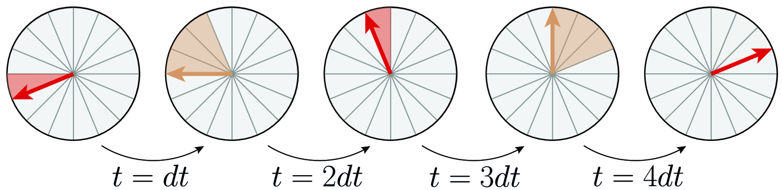
Figure 1: Schematic time-evolution of a single qubit oscillating between two quantum dots with distinct frequencies $\omega_{q,1}$ (red) and $\omega_{q,2}$ (yellow). We assume that the transfer rate between the dots is large enough that the electron instantaneously swaps position after each time step. Assuming that it starts in the first dot, the qubit rotates by one tile and ends up in the second dot after one time step. Next, it rotates by three tiles and comes back to the first dot. Finally at $t=4dt$, the qubit is back to its original position and has covered eight tiles. This leads to the conclusion that the resulting dynamics is a precession of the qubit at a frequency $\bar{\omega}_{q}=(\omega_{q,1}+\omega_{q,2})/2$.

III.1 Exchange-based homogenisation

III.1.1 Single-qubit gates on two electrons

One way to implement the example presented in Fig.˜1 is to make use of the exchange interaction as shown in Fig.˜2(a). The transfer rate corresponds here to the exchange coupling $J$. By turning on $J$, qubits in neighbouring quantum dots start to swap information. However, contrary to the previous example, this process is not instantaneous and will thus lead to a non-perfect homogenisation of the qubits resonance frequencies.

Let us add an oscillatory magnetic field with frequency $\omega=\bar{\omega}_{q}$. If the intuition exposed previously is right, one would expect to perform a perfect $X$-rotation on both qubits. This is confirmed by the numerics of Fig.˜3. Starting from the arbitrary initial state,

$$\ket{\psi_{0}}=\ket{0}\otimes\left(\sqrt{\frac{3}{4}}\ket{0}+\sqrt{\frac{1}{4}}\ket{1}\right),$$ (2)

we plot the expectation value of $\sigma_{z}$ over time for both qubits, at a finite $J=20\,\omega_{q}^{12}$ with $\omega_{q}^{12}=(\omega_{q,2}-\omega_{q,1})$, additionally choosing $\omega_{q}^{12}=\Omega$. These simulations are simply obtained by solving Schrödinger equation by time discretisation, using 10,000 time steps. The red and yellow faded lines respectively represent the full time-evolution of $\bra{\psi(t)}\sigma_{z}\otimes I\ket{\psi(t)}$ and $\bra{\psi(t)}I\otimes\sigma_{z}\ket{\psi(t)}$. These feature fast oscillations at a frequency $J$, which corresponds to the swapping of the qubits, and slower oscillations at frequency $\omega=\bar{\omega}_{q}$, which are triggered by the driving field. When sampling points from the red and yellow faded data every $2\pi/J$, one obtains the solid lines, which qualitatively look like an $X$ gate on both qubits. This means that, at finite but large enough $J$, the individual qubits indeed acquire the same effective frequency $\bar{\omega}_{q}$ and are thus resonantly driven by a single drive at $\omega=\bar{\omega}_{q}$.

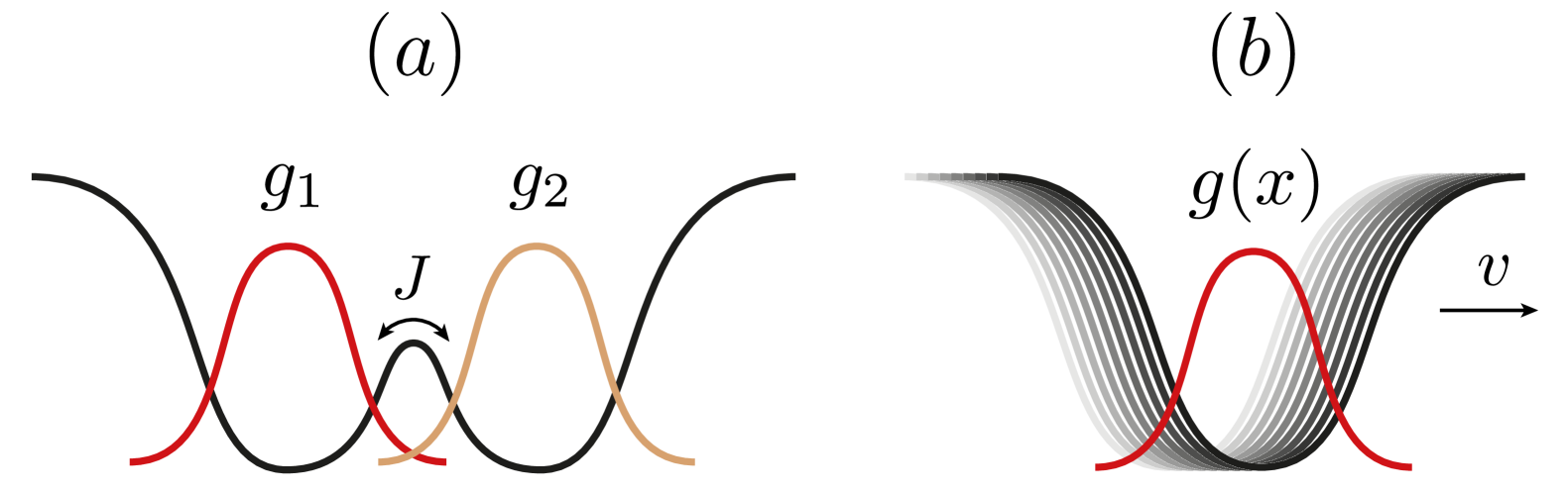
Figure 2: Physical implementations of the motion-based $g$-factor homogenisation. In (a), we consider two quantum dots with respective $g$-factors $g_{1}$ and $g_{2}$. The exchange coupling $J$ is used to homogenise the frequencies of the two electrons. This allows to reduce the number of distinct frequencies in the spectrum and thus reduce crosstalk. In (b) we use a completely different method in which we physically move the electron to perform the homogenisation. Here, the $g$-factor evolves continuously along the shuttling path. We find that this method is the most powerful as it can be generalised to an arbitrary number of qubits and scales better.

Unfortunately, the exchange interaction can entangle the qubits. Therefore, in order to implement an $X$ gate on both qubits without any additional entanglement creation, one must properly tune $J$ such that the qubits go back to their original positions in the time taken by the $X$ gates. This condition reads:

$$\frac{2p\pi}{J}=\frac{\pi}{\Omega},~~p\in\mathbb{N}$$

or equivalently:

$$J=2p\Omega,~~p\in\mathbb{N}.$$ (3)

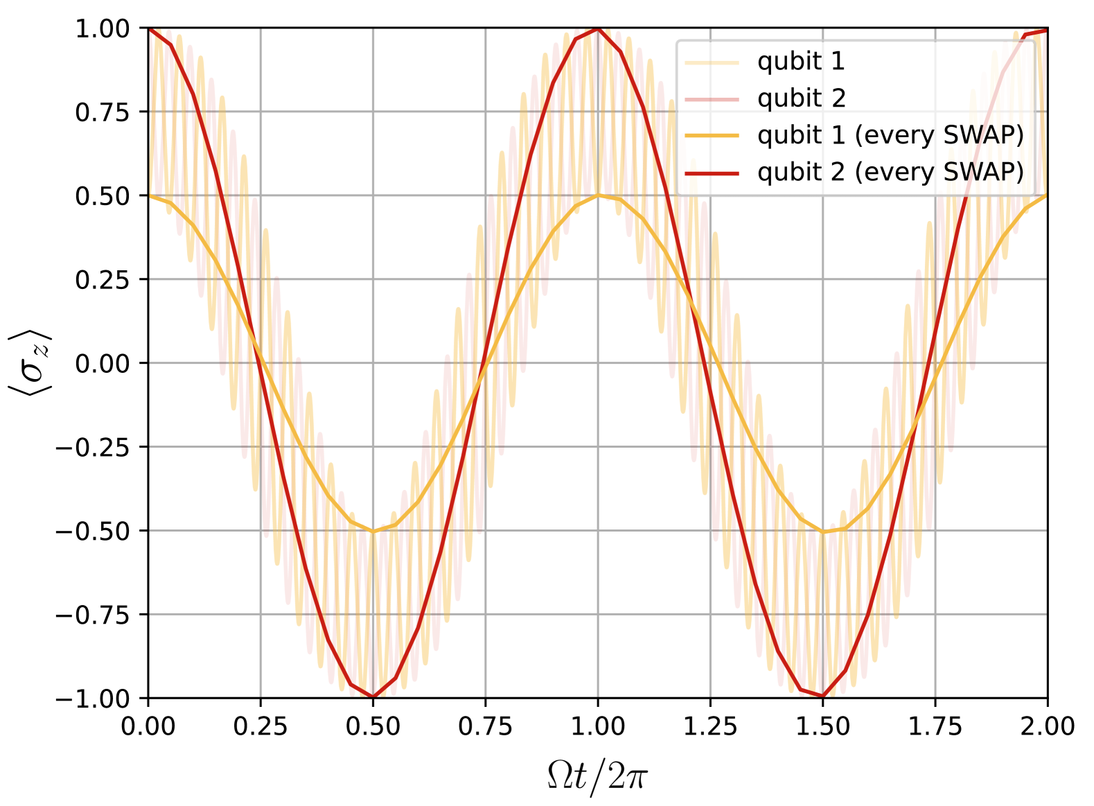
Figure 3: Time evolution of $\langle\sigma_{z}\otimes I\rangle$ and $\langle I\otimes\sigma_{z}\rangle$ under the two-qubit Hamiltonian of Eq.˜1. We set $\omega_{q}^{12}=\Omega$ and $J=20\,\omega_{q}^{12}$ where $\omega_{q}^{12}=(\omega_{q,2}-\omega_{q,1})$. The initial state is given in Eq.˜2. The faded lines correspond to the full time evolution, while the solid lines are obtained from sampling the full data every $2\pi/J$.

In order to further estimate the closeness of the implemented gate $U$ to the target unitary $U_{\text{target}}=X\otimes X$, one can evaluate the average single-qubit fidelity $\mathcal{F}$, defined as

$$\mathcal{F}=\frac{1}{4}\left|\mathrm{Tr}(U_{\text{target}}^{\dagger}\tilde{U})\right|^{2/n_{q}}$$ (4)

with $n_{q}=2$ and $\tilde{U}$ is a slightly modified version of the time evolution operator $U$ (where we removed known but unwanted $Z$ rotations) as explained in Appendix˜C. This quantity is dimensionless and thus only depends on the ratios of the three parameters dictating the dynamics of the two-qubit system: $J$, $\Omega$ and $\omega_{q}^{12}$. Only the difference between $\omega_{q,1}$ and $\omega_{q,2}$ matters, as their absolute values can be absorbed in a change of frame.

If the condition in Eq.˜3 is always enforced, one can expect the infidelity $1-\mathcal{F}$ to decrease to 0 when $J$ increases: this is confirmed by the numerics of Fig.˜4. One can also observe that when $\omega_{q}^{12}$ is decreased, the infidelity decreases as well: this is expected as the limiting case of $\omega_{q}^{12}=0$ should yield a null infidelity. Now, plugging in the experimental values from Table˜1, one approximately obtains $J/\Omega=100$ and $\omega_{q}^{12}/\Omega\gtrsim 1$. This results in an infidelity between $0.01\%$ and $0.1\%$.

In order to better understand what limits the fidelity here, we explore the Schmidt decomposition of $U$ in Appendix˜D. In particular, we show that at finite transfer speed $J$, the time evolution operator $U$ is indeed creating entanglement between the qubits, and cannot be decomposed into a product of two single-qubit gates.

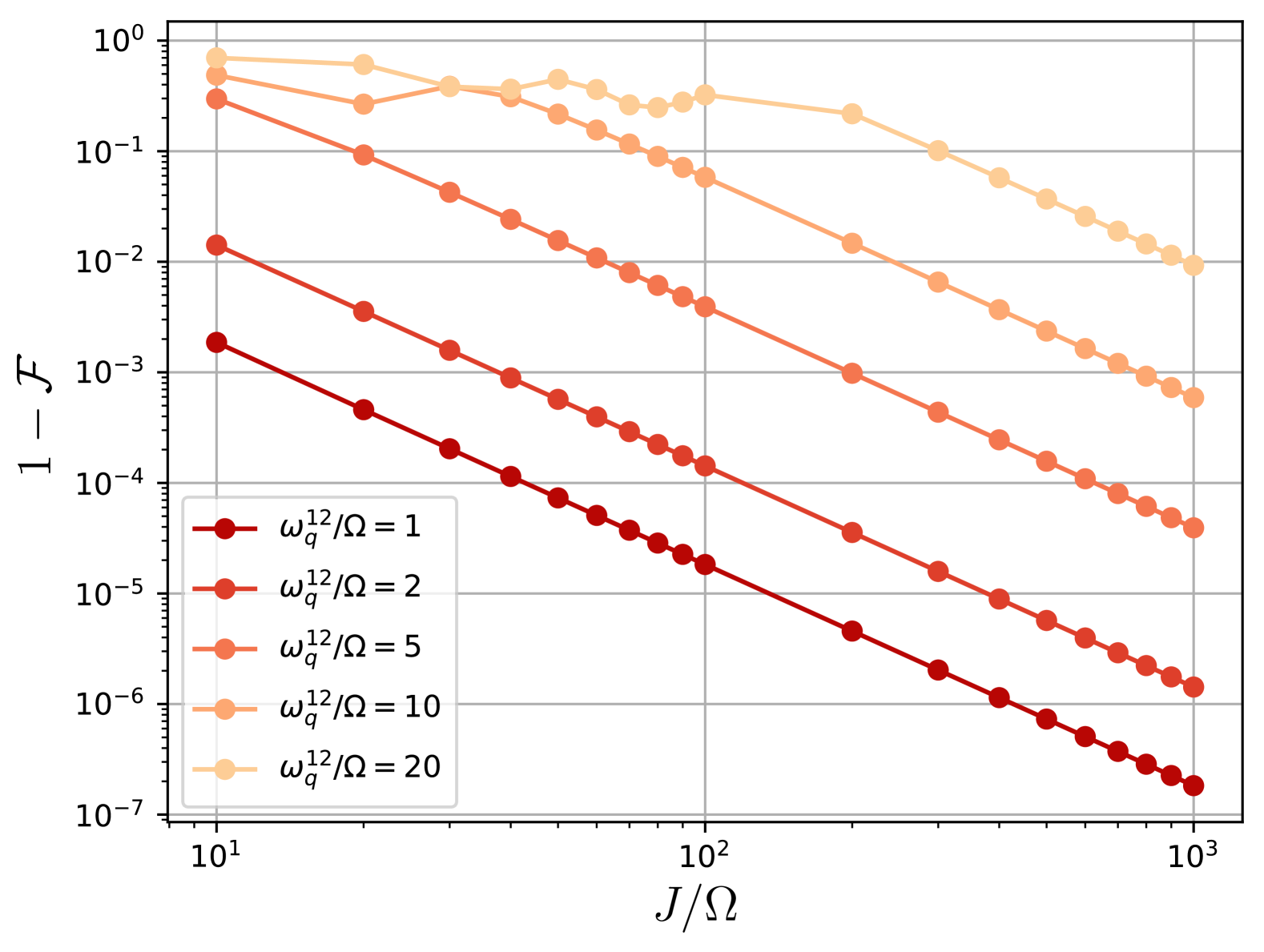
Figure 4: Infidelity of the swapping protocol. It is computed as the infidelity of implementing an $X\otimes X$ gate when driving two continuously-swapped qubits with frequencies $\omega_{q,1}$ and $\omega_{q,2}$ with a single driving tone at $\omega=\bar{\omega}_{q}$. The data is plotted against $J/\Omega$ and $\omega_{q}^{12}/\Omega$, where $J$ is the exchange coupling and $\omega_{q}^{12}=\omega_{q,2}-\omega_{q,1}$. $J$ is always chosen such that the condition in Eq.˜3 is satisfied.

As noted previously, the frequency homogenisation efficiency improves as one uses larger transfer rates. With the exchange coupling, one is limited to transfer rates of at most 10-1000 MHz in practice. However, by removing one electron from the DQD, one could rather leverage the tunnel coupling $t_{c}$ for electron transfer. This quantity can reach 1-10 GHz [37], which should lead to better global control fidelities. Moreover, contrary to the exchange-based homogenisation, this method does not create any electron-electron entanglement, which is a limiting factor to our fidelity. We investigate this in Appendix˜E.

III.1.2 Single-qubit gates on more than two electrons

The extension of the SWAP-based scheme to more than two qubits is not trivial. Indeed, one would naively think that turning on the $J$-coupling between all adjacent dots would produce the same desired outcome. Unfortunately, multi-qubit SWAP gates are not implemented by simply turning on all $J$-couplings. Rather, one could think of implementing a multi-qubit SWAP gate by decomposing it into two-qubit SWAPs, which could be performed by turning the $J$-couplings on and off in an alternate fashion. If this method theoretically works, it is however impractical.

One of the most significant sources of errors in implementing SWAP gates is charge noise, which arises from two-level fluctuators (TLFs) [38, 39, 40]. These TLFs lead to unknown modifications in the exchange coupling [29, 28, 27], leading to timing errors that reduce the fidelity. When decomposing a multi-qubit SWAP gate into two-qubit SWAPs, a large number of sequential SWAPs between different qubits are required. This results in an exponential decrease in overall fidelity with the number of SWAPs, rendering the protocol impractical. However, in the two-qubit case, we only need to turn the exchange coupling on and off once, so the timing error only affects the process a single time. Moreover, since the exchange is active for an order of microseconds, charge fluctuations on this timescale should average out the variations of the exchange coupling, leading to higher fidelity [29]. Finally, it is important to note that as charge noise modifies the exchange coupling $J$, it will lead to a violation of the condition in Eq.˜3. As this paper focuses on addressability, the impact of charge noise on our scheme is left for further study.

III.2 Shuttling-based homogenisation

III.2.1 Single-qubit gate on a single electron

In the previous section, we focused on a mechanism that allows for a qubit to oscillate between two regions of fixed $g$-factors. In this section, we advocate for the use of a more powerful mechanism, which leads to a broader exploration of the $g$-factor landscape: electron shuttling. Here, the electron is physically moved thanks to the electrical control of the trapping potential and can thus explore a continuous landscape of $g$-factors as illustrated in Fig.˜2(b). Moreover, this scheme can easily be generalised to more than two qubits, as multiple electrons can be shuttled at the same time without any entanglement being generated between them.

There are two main ways to perform electron shuttling: the bucket brigade mode [32, 41, 42, 43], in which the electron is moved from one dot to another by altering the detuning between them and the conveyor-belt mode [33, 20, 25, 44, 34, 45], in which it is the trapping potential itself that moves, carrying the electron with it. Here, we will focus on the latter as it is more advantageous in terms of scalability [20, 34], and recent experiments showed that coherent spin shuttling in Si/SiGe can be achieved with fidelities as high as $99.99\%$ for gate-to-gate distance and around $99\%$ for a distance of 10 $\mu$m [34]. As in the previous sections, an electron shuttled in a region of varying $g$-factor will acquire an average effective frequency if shuttled fast enough, with the difference that we are now considering a continuously varying $g$ (see Eq.˜12). This frequency narrowing phenomenon had in fact already been observed in the context of shuttling, but had never been used for single-qubit addressability [25].

More precisely, during the gate time $T=\pi/\Omega$, an electron with trajectory $x(t)$ will obtain the homogenised $g$-factor $\bar{g}$ given by,

$$\bar{g}=\frac{1}{T}\int_{0}^{T}g(x(t))dt.$$ (5)

Contrary to the exchange- and tunnel-based protocols, it seems that we now require a perfect knowledge of $g(x(t))$ at each time $t$ in order to find the drive frequency. While this would be quite challenging, one can rather directly determine the drive frequency by shuttling the electron along $x(t)$ and by sweeping the frequency of the drive $\omega$ until resonance with the qubit is obtained [46]. One can then deduce $\bar{g}$ from $\omega$ as $\omega=\bar{g}B_{0}$.

However, depending on the shuttling trajectory $x(t)$, such characterisation might not be needed. Suppose that we let the electron explore dots without repetitions, e.g. by shuttling it on a straight line for a time $T$. As the travelled distance increases, the homogenised $g$-factor $\bar{g}$ given by Eq.˜5 will tend towards the device average $g$-factor $g_{0}$. For a sufficiently long distance, we expect that no calibration is needed and that the sole knowledge of $g_{0}$ is required. This observation allows us to propose two different driving modes: mode I, for which we drive the qubit at a frequency $\omega=\bar{\omega}_{q}=\bar{g}B_{0}$; and mode II, where $\omega=\omega_{0}=g_{0}B_{0}$.

In the rest of the section, we study the evolution of the infidelity associated with both driving modes. Let us suppose that we shuttle a qubit back and forth and that its movement is described by a triangle wave, recursively defined as:

$$x(t)=\begin{cases}d/2-vt,&\text{if}\ t<d/v\\ -3d/2+vt,&\text{if}\ d/v\leq t<2d/v\\ x(t-2d/v),&\text{if}\ t\geq 2d/v\end{cases}$$ (6)

with $d$ representing the distance travelled by the electron for one way and $v$ is its (constant) shuttling speed. Furthermore, we fix $\Delta g=10^{-3}$ to address cases of higher frequency crowding.

To guide the analysis of the numerical simulations of the infidelity of our protocol, it is important to note that it suffers from two main sources of errors: the homogenisation error and the error arising from off-resonant driving. While the latter is well understood and explained by the Rabi model, we need to describe the impact of $v$ and $d$ on the former. In Fig.˜5, we use Gaussians centred around the mean $g$-factor to symbolise the quality of the shuttling-based homogenisation (in the spirit of frequency narrowing). Considering some distance $d$, and a constant speed $v$ in Fig.˜5 (a), the homogenisation is not perfect as illustrated by the wide distribution around the $g$-factor associated to the drive frequency $\omega=\bar{g}_{d}B_{0}$. While keeping $d$ fixed, increasing $v$ in Fig.˜5 (b) yields a better homogenisation as explained in previous sections. The faded Gaussian, corresponding to a slower speed, is thus less peaked. Keeping $v$ fixed, choosing a distance $d^{{}^{\prime}}>d$ in Fig.˜5 (c) reduces the quality of the protocol as the electron has to explore more dots. Moreover, as $d\rightarrow\infty$ we have $\bar{g}_{d}\rightarrow g_{0}$, which explains the shift of the mean frequency. The faded Gaussian, corresponding to a smaller distance, is therefore more peaked but its mean is farther from $g_{0}$.

We are now ready to study the infidelity of an $X$ gate performed on a qubit as a function of $d$, for different speeds $v$ and drive amplitudes $\Omega$ as plotted in Fig.˜6 . The distance $d$ ranges from $100$ nm (the interdot distance) to the maximum distance the electron can travel during the gate time i.e. $L=vT$. The infidelity measure is the same as for the exchange-coupling-based scheme – further details on this metric and its numerical simulation can be found in Appendix˜C. Each data point is obtained by averaging 20,000 instances of $g$-factors generated using the method presented in Appendix˜A.

For mode I (top of Fig.˜6), in which we drive at the mean frequency $\omega=\bar{g}_{d}B_{0}$ ($\bar{g}_{d}$ being the mean $g$-factor for a distance $d$), the infidelity increases with $d$ for fixed $v$ and $\Omega$. This is characteristic of a degradation of the homogenisation in the presence of a larger number of distinct $g$-factors, as explained before. Then, we notice that the curves can be grouped by their speed $v$, with the infidelities for $v=50$ m/s (red) approximately an order of magnitude smaller than for $v=10$ m/s (yellow), in agreement with our predictions. The larger the speed (or transfer rate) $v$, the better the homogenisation. Finally, we note that within each group a change in $\Omega$ (solid versus dashed lines) does not have much impact on the infidelity, at least in the experimentally relevant parameter regime we study. Indeed, when looking at the Rabi model, the value of $\Omega$ does not affect the infidelity when driving on resonance.

For mode II (bottom of Fig.˜6), in which we drive at $\omega=g_{0}B_{0}$, the infidelity decreases with $d$ unlike mode I. Indeed, as $d$ gets larger, $\bar{g}_{d}$ tends to $g_{0}$ as showed before, thereby reducing the detuning between the drive and qubit frequency. While we can also group the curves in pairs here, it is now the driving amplitude that discriminates them. Suppose that $\Omega$ is fixed, increasing the speed $v$ only allows for the reduction of the homogenisation error. As we are dominated by the off-resonant driving error here, changing $v$ has a negligible impact. Within the Rabi model, this type of error solely depends on the ratio $|\omega-\omega_{q}|/\Omega$. The larger the ratio, the higher the fidelity. That is why the infidelity decreases as $\Omega$ increases.

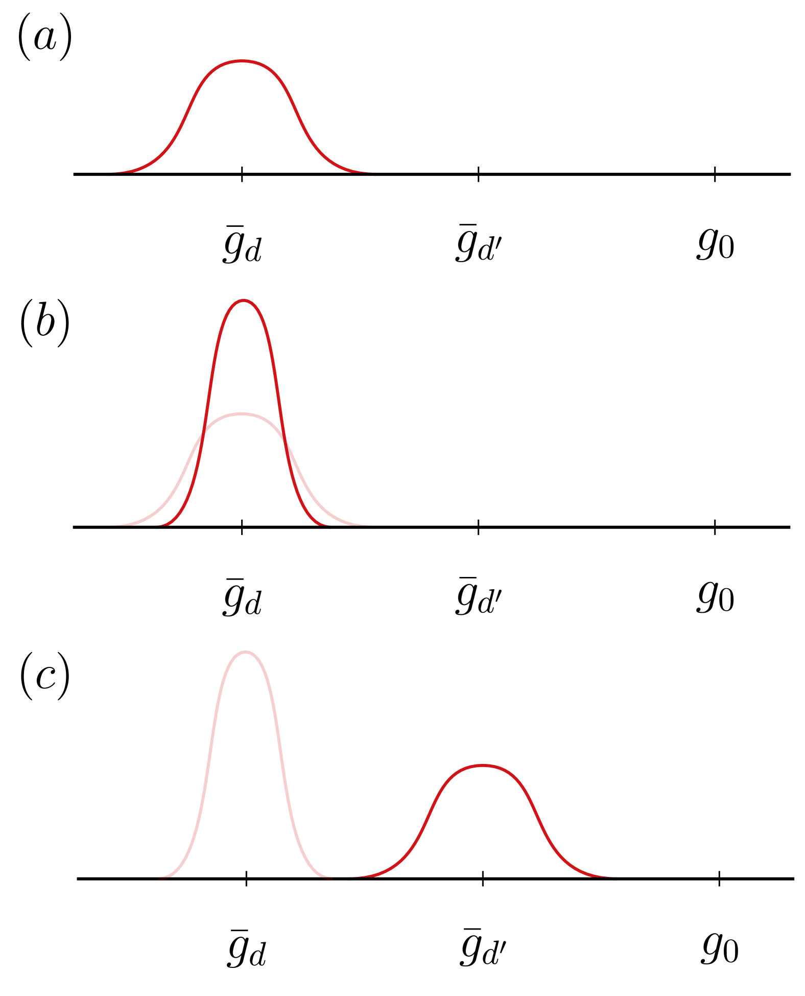
Figure 5: Illustration of the impact of speed and explored distance on the quality of the homogenisation process. (a) Wide distribution around the mean $g$-factor representing an imperfect homogenisation. (b) Increasing the speed (i.e. the transfer rate) while keeping the explored distance fixed improves the quality of the homogenisation as explained before. The faded Gaussian is plotted for comparison. (c) Increasing the shuttled distance while keeping the same speed deteriorates the homogenisation as the electron explores more dots. The shift of the mean frequency manifests the fact that $\bar{g}_{d}\rightarrow g_{0}$ as $d\rightarrow\infty$.

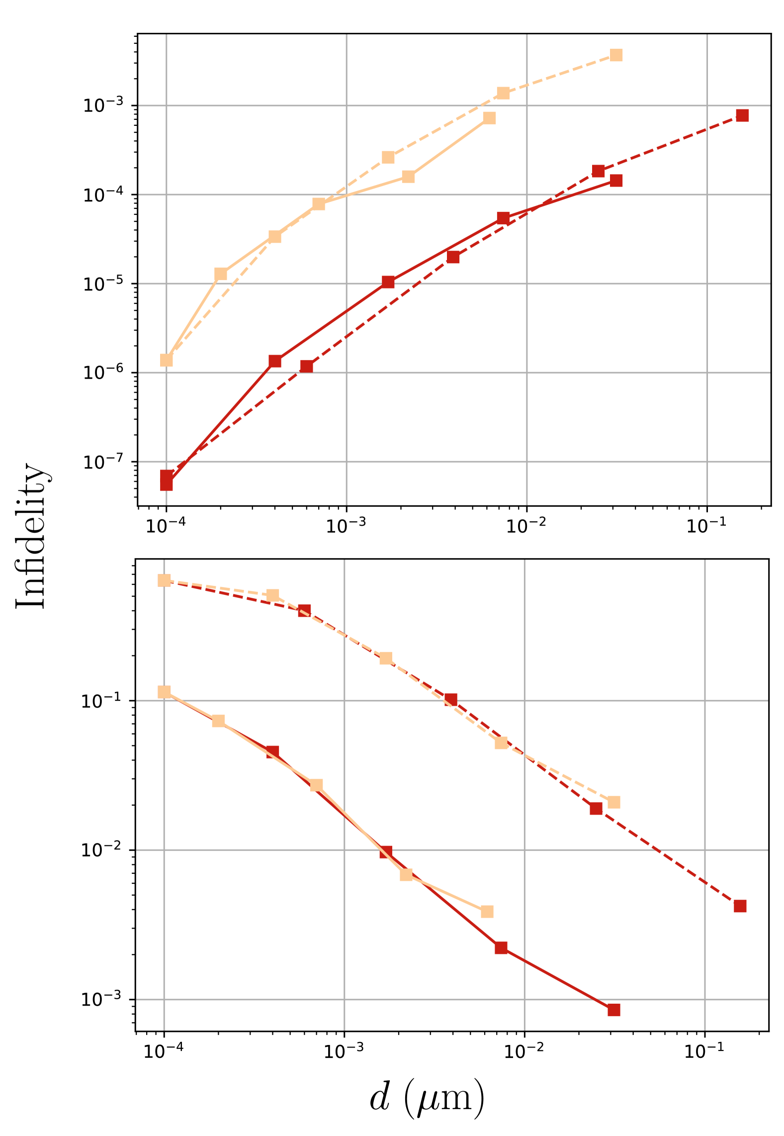
Figure 6: Infidelity of the shuttling-based protocol for modes I (top) and II (bottom) as a function of the distance $d$, the speed $v$ and the drive amplitude $\Omega$. These infidelities are obtained by performing 20,000 Monte-Carlo simulations with random instances of the $g$-factor landscape. The yellow and red lines correspond to $v=10$ m/s and $v=50$ m/s respectively. The solid lines indicates that $\Omega=5$ MHz, while $\Omega=1$ MHz for the dashed lines.

As our aim is to characterise the quality of the homogenisation, shuttling errors were not included in the previous simulations. If they were, we would need to consider a tradeoff between shuttling noise and homogenisation error for mode II. Indeed, as the distance increases, the infidelity of our protocol decreases while shuttling noise would increase. One would need to find a sweet spot balancing the impact of these two error sources. For mode I, increasing $d$ decreases the infidelity, so including shuttling noise would only aggravate the situation. As a reminder, recent experiments in Si/SiGe showed per-increment shuttling fidelities being progressively reduced from $10^{-3}$ to $10^{-4}$ [32, 33, 34]. As one hop can be implemented in $\sim$10 ns (assuming an interdot distance of 100 nm and a shuttling speed of 10 m/s), the resulting overall shuttling noise over one $X$ gate (lasting $1~\mu$s for $\Omega=1$ MHz) reaches at best $10^{-2}$ with current technologies. However, the task of low-noise shuttling is receiving rapidly increasing attention, notably with recent proposals suggesting that $g$-factor disorder might help improve shuttling fidelities rather than hinder them [47]. We will thus assume that these will keep improving.

Additionally, while the results presented in this section are dependent on how the $g$-factor landscape is defined, the homogenisation principle should work for any model. However, it is worth noting that this scheme only performs well in the case of low frequency dispersion $\Delta\omega_{q}$ i.e. at low magnetic field $B_{0}$ and low $g$-factor dispersion $\Delta g$. This is analogous to the observations of Fig.˜4 for the case of exchange oscillations, in which the infidelity rapidly degraded with the frequency spreading $\omega_{q}^{12}$. We will confirm this statement for shuttling as well in Section˜IV.

Finally, note that we assumed here (and in the rest of the paper) that the drive amplitude $\Omega$ is homogenous over the shuttling path, which can be quite challenging to achieve but not impossible [12]. We however confirmed with additional numerics that our scheme performs the same in the presence of a non-uniform driving field. Namely, the resonant frequency of a shuttled qubit would still be the average $g$-factor over the shuttling path and the resulting infidelity would be identical to the case of uniform $\Omega$. The only distinction resides in the gate time, now defined as $T=\pi/\bar{\Omega}$, where $\bar{\Omega}$ is the average Rabi frequency over the shuttling path.

III.2.2 Single-qubit gates on more than one electron

Although we verified here that shuttling could advantageously be used to homogenise $g$-factors in the simplest case of a single qubit, this method can trivially be extended to higher qubit counts. Unlike the previously presented exchange-based scheme, conveyor-belt shuttling [33, 20] can conveniently be utilised to synchronously shuttle large groups of qubits with no increased resource overhead and without prohibitive fidelity reductions. Indeed, this mode of shuttling uses four input voltages only to create a moving sine wave, whose minima can hold the shuttled qubits and displace them altogether. Clusters of same-frequency qubits can thus be formed by shuttling qubits around loops, such that all qubits in the loop explore the same $g$-factor landscape.

III.2.3 Extension to two-qubit gates

While the focus of this paper is on the use of frequency homogenisation to perform global single-qubit gates, our protocol can be generalised to two-qubit gates as well. With silicon-spin qubits, these can be implemented by turning on the exchange interaction between neighbouring electrons. Depending on additional parameters e.g. the existence of a sufficient energy separation between the electrons or the application of a resonant drive, various kinds of gates can be implemented. These include $\sqrt{\text{SWAP}}$, CZ gates and CROT gates [48]. We will here focus on the latter as it requires the use of a drive, therefore making its description a natural extension of the single-qubit case.

More precisely, a CROT gate is a rotation around an axis in the $xy$ plane of the spin of a first electron, conditional on the state of a second electron. To implement it, the exchange interaction $J$ must be turned on but kept small compared to the qubits’ energy separation, which we denote as $GB_{0}$. In this parameter regime, the degeneracy between the basis states of the two qubits is lifted, enabling the selective targetting of a specific energy transition with a driving pulse. By setting the drive frequency at the energy splitting of the $\ket{10}$-$\ket{11}$ transition, a CROT gate is implemented in a time $\pi/\Omega$ (when $J\ll GB_{0}$). This frequency is given by [2, 49, 50, 51]:

$$\omega=\frac{1}{2}(\omega_{q,1}+\omega_{q,2}-J+\sqrt{J^{2}+(\omega_{q,1}-\omega_{q,2})^{2}})$$ (7)

where $\omega_{q,i}=g_{i}B_{0}$ is the intrinsic frequency of qubit $i\in\{1,2\}$.

Like in the single-qubit-gate case, when many qubits are present in the device, it may prove challenging to selectively target pairs of qubits due to frequency crowding. Here we show that this can be mitigated by applying our shuttling-based homogenisation scheme in the same fashion as before. We thus consider two electrons evolving on two parallel shuttling tracks characterised by distinct $g$-factor profiles $g_{1}(x_{1})$ and $g_{2}(x_{2})$. A large frequency shift $GB_{0}$ is applied between the shuttling tracks i.e. by using a micromagnet or magnetic materials. Both electrons are synchronously shuttled back and forth on their respective shuttling track over a distance $d$ (see Eq.˜6), with a small exchange interaction $J\ll GB_{0}$ always turned on between them. The effect of shuttling is to homogenise the respective $g$-factors of the electrons, leading them to acquire the effective frequencies $\bar{\omega}_{q,1}$ and $\bar{\omega}_{q,2}$. In the light of the previous section, two driving modes are conceivable. Driving mode I consists of driving at the exact means:

$$\omega_{I}=\frac{1}{2}(\bar{\omega}_{q,1}+\bar{\omega}_{q,2}-J+\sqrt{J^{2}+(\bar{\omega}_{q,1}-\bar{\omega}_{q,2})^{2}})$$ (8)

which requires a precise knowledge of the $g$-factor landscape. In contrast, in driving mode II we drive at the device averages:

$$\omega_{II}=\frac{1}{2}((2g_{0}+G)B_{0}-J+\sqrt{J^{2}+(GB_{0})^{2}})$$ (9)

which is agnostic of the details of the $g$-factor landscapes. Given the experimental challenge that implementing two-qubit gates while shuttling would represent, we decide to solely focus here on the more experimental friendly driving mode i.e. mode II.

The results of such an approach are presented in Fig.˜7. We observe like in Fig.˜6 (bottom) that the infidelity decreases with the shuttling distance $d$. Indeed $\omega_{II}$ becomes a better and better estimate of the optimal driving frequency $\omega_{I}$. Contrary to the single-qubit case however, the infidelity saturates at large $d$ instead of keeping decreasing: this is because even the static and exactly-resonant implementation of the two-qubit gate is imperfect (e.g due to crosstalk with other energy transitions, see [2, 49] for details). This source of infidelity can be tamed by increasing $G$ – since the condition $J\ll GB_{0}$ would become better enforced – or by carefully choosing $\Omega$ in order to synchronise the resonant and off-resonant rotations [50]. It is worth noting that increasing $v$ reduces the infidelity too, since it improves the quality of the shutting-induced homogenisation. Finally, note that the scheme we here advocate for only works when electrons are shuttled in separate tracks that are well separated in frequency (large $G$). If $G$ was null or if the electrons were to be placed on the same shuttling track, the resulting operation would be an $XX$ gate.

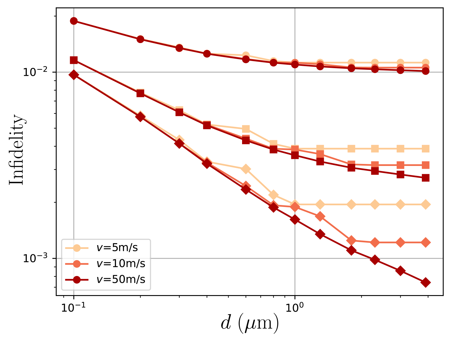
Figure 7: Infidelity of a CNOT gate implemented while shuttling the qubits so as to homogenise their respective $g$-factors. Lighter to darker colours correspond to increasing shuttling speeds. Each triplet of curve (from top to bottom: circles, squares, diamonds) is characterised by a distinct frequency gradient $GB_{0}$ between the shuttling rails, respectively 500 MHz, 1 GHz and 2 GHz.

IV Applications

We showed in the previous section that the shuttling-based protocol was the more scalable one. Indeed, it can be applied to multiple electrons without generating entanglement between them and guarantees a high single-qubit gate fidelity while only using a limited number of electrodes. In this section, we thus focus on this protocol and evaluate its performance for the global control of single-qubit gates in a realistic setting.

IV.1 Problem statement

Given the model presented in Section˜II, we wish to perform a high-fidelity $X$ gate on $n_{t}$ targets qubits while keeping the other $n_{q}-n_{t}$ qubits idle by using a global driving field.

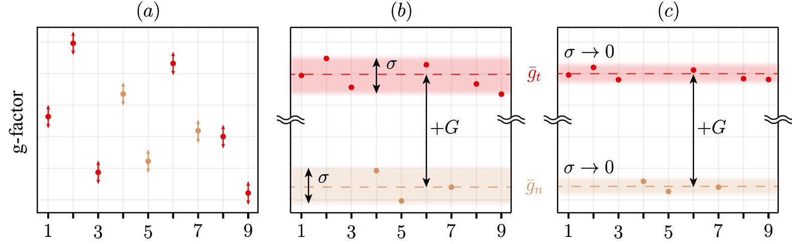
Figure 8: Illustration of the global control workflow. We wish to perform an $X$ gate on the target qubits (red) while leaving the non-target qubits (yellow) idle. (a) Given an initial $g$-factor distribution, we shuttle qubits so as to homogenise their $g$-factors. The arrows describe the $g$-factor landscape explored by each electron and the central dots correspond to the resulting mean values. The quality of this process is in particular dependent on the shuttling speed $v$ (see Fig.˜5). (b) Using micromagnets or superconducting lines, we apply a magnetic field which effectively shifts the $g$-factors of the targets with respect to the non-targets by $G$ as explained in the main text. The target and non-target qubits homogenised $g$-factors are now separated and spread around their means $\bar{g}_{t}$ and $\bar{g}_{n}$ (dashed lines). The standard deviation of this distribution is given by $\sigma$ (red and yellow shaded areas). (c) Our shuttling-based homogenisation allows us to decrease $\sigma$ by increasing the shuttling distance $d$ (see Fig.˜5(c)). In the limit of large $d$, every qubit within the red and yellow shaded areas acquire the same $g$-factor, thereby reducing the spectrum to only one target and one non-target frequencies. Alternatively, $\sigma$ can be negated by further frequency engineering, namely by applying a distinct $G$ to each qubit.

The general workflow we adopt is the following (see Fig.˜8): starting from an initial distribution of $g$-factors $(g_{i})_{1\leq i\leq n_{q}}$, we apply both our shuttling-based homogenisation protocol and additional electromagnetic fields (e.g. Stark shift, global magnetic field gradients) to reduce the frequency spectrum to essentially two $g$-factors $\bar{g}_{t}=g_{0}+G$ and $\bar{g}_{n}=g_{0}$, corresponding to the mean target and non-target $g$-factors respectively after homogenisation. In some cases, there will remain a distribution of target and non-target $g$-factors around $\bar{g}_{t}$ and $\bar{g}_{n}$, but we will ensure that the width $\sigma$ of such a distribution is small compared to $G$. $\sigma$ is controlled by the shuttling distance $d$: the larger the distance, the smaller $\sigma$ is. In contrast, $G$ is adjusted via the application of aforementioned electromagnetic fields. Note that the shuttling speed $v$ has no impact on $\sigma$ (which quantifies the distance between the homogenised $g$-factors and their means $\bar{g}_{t}$ and $\bar{g}_{n}$). $v$ only influences the quality of each homogenisation (see Fig.˜8).

Thereon, we send a driving tone at (almost) resonance with the target qubits: $\omega=\bar{g}_{t}B_{0}$. Ideally, when $G$ is large and $\sigma$ is small, the non-targets are left almost idle while each target rotates at a rate $\Omega\approx\bar{g}_{t}B_{1}$. In reality, each target rotates around a slightly tilted axis as $\sigma$ is finite. Besides, the non-targets may experience some crosstalk due to finite $G$. In order to mitigate it, we additionally tune $\Omega$ such that the driving tone induces a $\pi$ rotation on the targets qubit, but a $2\pi$ rotation on the non-targets. This is explained in Appendix F.

We will compare this workflow to a state-of-the-art implementation of global single-qubit gates [19, 14], which leverages the same ingredients as above but without our shuttling-based homogenisation. For this reason, it is in general not possible in this case to reduce the spectrum to only two main frequencies like before ($\sigma$ would be too large). Rather, frequency crowding and frequency separation are dealt with by the sole application of electromagnetic fields, namely by placing the qubits frequencies into (more than two) same-frequency bins. This way the minimum frequency spacing does not decrease with the system size, providing a solution to the frequency crowding issue. The driving pulse has to be composed of multiple driving tones, separated by a frequency distance equal to the bin spacing $2\delta\omega_{q}$. This relatively low distance can be a source of crosstalk, whose effect is mitigated by tuning the drive strength $\Omega$ like before (see Appendix F). We will refer to this general method as the binning technique.

More concretely, we will focus on two architectures suited for different eras: the near-term 2$\times$N [21] and the long-term looped pipeline architectures [24]. Exploring these two architectures allows us to survey the efficacy of our scheme for both the NISQ and fault-tolerant eras. Note however that 2$\times$N arrays of qubits will also be relevant in the fault-tolerant regime as we explored in [21, 22].

In all the following, we will assume a varying number of target qubits $n_{t}$ and set the number of non-target qubits to $n_{n}=n_{t}-2$ as an example. The $g$-factor dispersion $\Delta g$ is set to $10^{-3}g_{0}$ or $10^{-2}g_{0}$, which we will denote as low and high interface roughness respectively. The maximum Stark shift $\delta g$ is set to $\Delta g/10$. Besides we will use a drive strength $\Omega$ around 5 MHz (taking into account the synchronisation of the target and non-target qubits rotations, as explained in the previous paragraphs and in Appendix F). When evaluating the performance of our proposal, we will assume a constant magnetic field $B_{0}=0.1$ T to minimise frequency spreading and facilitate our homogenisation protocol. In contrast, for the binning technique, we will set $B_{0}=1$ T to maximise the frequency shift allowed by Stark shift, which sets the bins separation. As such we are comparing both schemes when they are performing best. In addition, we will separate the targets and non-targets by a frequency shift $GB_{0}=300$ MHz. Assuming that targets and non-targets are on distinct shuttling tracks that are separated by 100 nm (as it will be the case in the following), this translates into a magnetic field gradient of 0.1 mT/nm. This is comfortably below demonstrated gradients induced by micromagnets, around 0.8 mT/nm [52]. As for the shuttling distance and speed, we will consider two distinct parameter regimes that will depend on the architecture: $v=10$ m/s and $d=3\;\mu$m (2$\times$N); or $v=50$ m/s and $d=20\;\mu$m (looped pipeline). We will comment on the choice of these parameters in Appendix˜G. The performance of each technique is evaluated by running 10,000 Monte Carlo simulations with randomly-generated $g$-factor profiles. In each instance, we use the same fidelity measure as before: details on our numerics can be found in Appendix˜C. Shuttling noise will still be neglected in the present study in order to focus on qubit addressability.

IV.2 Performance on the 2$\times$N array

The first architecture we consider corresponds to the easiest extension of a 1$\times$N array of quantum dots. Despite its simplicity, it has been showed that one can reliably implement error correction on this architecture [21]. However, here we are concerned with a more restricted version of the architecture in which we require the second row of the 2$\times$N array to be empty as shown in Fig.˜9.

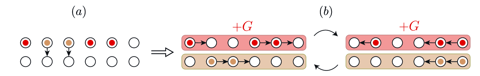
Figure 9: Illustration of the shuttling-based protocol for a 2$\times$N array. Starting with all the qubits on the top row in (a), we move the non-targets to the bottom row to physically separate the two types of qubits. Then, thanks to superconducting lines or micromagnets we apply a large magnetic field gradient between the rows (shaded areas) in (b). This magnetic field gradient can also be seen as shifting the $g$-factors of the electrons on the top row by $G$. Finally, the electrons are shuttled back and forth in lines to homogenise their $g$-factors.

As explained in the previous section, our first goal is to simplify the frequency spectrum, namely to only retain one main target $g$-factor $\bar{g}_{t}$ and one main non-target $g$-factor $\bar{g}_{n}$. To do so, we first spatially separate the targets from the non-targets by transferring the non-target qubits to the bottom row (Fig.˜9(a)). In addition to this, we apply a magnetic field gradient between the rows, e.g. by placing micromagnet or a superconducting wire parallel to the array. This generates the desired frequency separation $GB_{0}$. At this stage however, the target and non-target $g$-factors are scattered around their mean values (respectively $\bar{g}_{n}=g_{0}$ and $\bar{g}_{t}=g_{0}+G$). To lower the standard deviation $\sigma$ of these dispersions, we shuttle both rows of qubits back and forth (Fig.˜9(b)). This results in reducing $\sigma$ by homogenising the $g$-factor landscape as illustrated in Fig.˜8. Target qubits can now be driven close to resonance by sending a driving pulse at $\omega=(g_{0}+G)B_{0}$. This is reminiscent of the driving mode II we explored in Section˜III.2, where qubits are not driven at exact resonance, but rather at a known frequency that is agnostic of the details of the $g$-factor landscape ($\omega$ only depends on the device average $g$-factor $g_{0}$ and the set magnetic field gradient $GB_{0}$). As such, the infidelity is arising from two main contributions: the slightly off-resonant driving of the target qubits and the crosstalk between targets and non-targets. Note that in the present scheme, it is not feasible to use the driving mode I (where each target qubit is driven at exact resonance). Indeed, the leftmost and rightmost qubits of the top row do not experience the same $g$-factor landscape, yet their resulting effective $g$-factors are both too close to $\bar{g}_{t}$ to differentiate them and drive them with two distinct driving tones.

In Fig.˜11, we compare this protocol to the binning technique, as explained in the previous section. We will focus on the left panel, corresponding to a shuttling speed $v=10$ m/s and a distance $d=3\;\mu$m i.e. spanning 30 quantum dots. This scenario is realistic for the near term [34]. We find that in the case of low interface roughness (solid lines) our shuttling protocol (orange) quickly outperforms the binning scheme (yellow). More specifically, it yields a per-qubit infidelity around $0.3\%$ i.e. under the surface code threshold, which the binning scheme fails to provide. We however observe an opposite behaviour in the case of high interface roughness (dashed lines), where the binning scheme yields a desirable sub-threshold single-qubit infidelity, far below the one obtained with shuttling. This is because the homogenisation of the $g$-factors becomes more demanding at large $\Delta g$, requiring unfeasible shuttling speeds or drive strengths to compensate for the wider dispersion when shuttling. In contrast, the binning scheme performs well at high interface roughness, owing to a greater interbin spacing arising from a larger Stark shift $\delta g=\Delta g/10$. Note however that contrary to our shuttling scheme, the binning scheme requires a perfect knowledge of the $g$-factor landscape and a reliable tunability via Stark shift. Besides, we expect the interface roughness to decrease over time as manufacturing technologies improve.

An additional interesting feature one can note is that the average single-qubit fidelity as defined in Eq.˜4 decreases when loading more qubits into the device with our shuttling scheme. In contrast, it grows with the binning scheme. We can explain this by noting that in the first case we are not increasing the number of driving tones with the number of qubits, while in the second case, a new driving tone should be added every time a new bin is created. This leads to an increase of the crosstalk between target qubits. At sufficiently large numbers of qubits, both infidelities become stationary however, meaning that both schemes can address the frequency crowding issue, albeit in different parameter regimes.

IV.3 Performance on the looped pipeline architecture

The second architecture was suggested by Cai et al. as a way to increase the logical-level connectivity between 2D error-correcting codes, or encode 3D error correction structures within a strictly 2D device [24]. This amelioration is carried out by shuttling data and ancilla qubits in separate loops that occasionally meet for the implementation of two-qubit gates. By placing multiple electrons in each loop, out-of-plane layers of error correcting codes are effectively stacked together (see Fig. 4 of [24]). Throughout the normal execution of stabiliser cycles, data qubits frequently need to be collectively addressed by a single-qubit Hadamard gate while leaving ancilla qubits idle.

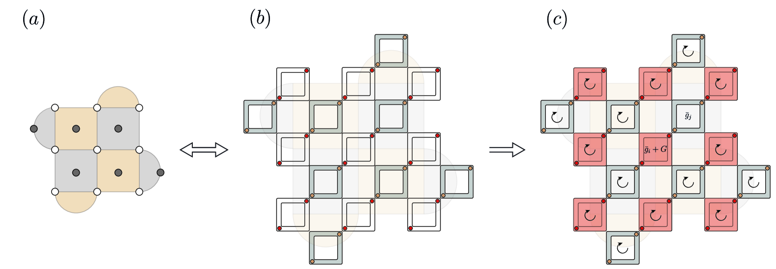
Figure 10: (a) Schematic representation of the $3\times 3$ surface code with data and ancilla qubits represented in white and grey respectively. (b) Implementation of the $3\times 3$ surface code within the looped-pipeline architecture with white and grey loops representing data and ancilla loops respectively. Note that $n$ electrons ($n=2$ here) can populate each loop in order to encode more than one surface code patch as explained in the main text. Red and yellow electrons represent target and non-target qubits respectively. (c) Implementation of single-qubit gates using our shuttling-based homogenisation protocol. During each stabiliser cycle, we wish to perform single-qubit gates on the data loops while leaving the ancillas idle. By shuttling the electrons around loops we homogenise their $g$-factors and reduce the number of distinct frequencies from $17n$ (with $n$ being the number of electrons per loop) to 17 (number of loops). In order to further reduce crosstalk, we adopt the strategy presented in Fig.˜8 leveraging superconducting lines/micromagnets to differentially shift the $g$-factors of the targets (red shaded area) with respect to the non-targets. We denote the $g$-factor of the data qubits as $\bar{g}_{i}+G$ and that of the ancillas as $\bar{g}_{j}$. Note that, one could tailor the field generated by the micromagnets such that every target obtains the same $g$-factor $G_{0}$, which yields an even higher fidelity as seen in Fig.˜11.

In Fig.˜10, we represent the looped pipeline architecture in the case of two stacked $3\times 3$ surface codes patches. Data and ancilla qubits (and loops) are represented in white and gray respectively. As qubits go around in loops, they acquire an effective frequency equal to the mean frequency of their respective shuttling track as per the observations of the previous section.

Contrary to the previous architecture we considered, target and non-target qubits are inherently spatially separated, which simplifies their addressability. In order to separate them in the frequency spectrum, we again apply a magnetic field gradient between the target and non-target shuttling tracks. Nonetheless, thanks to the less constrained architecture, we here have more flexibility in the choice of the applied field. Namely, we can distinguish two realistic scenarios. In the simplest one, the same frequency shift $GB_{0}$ is applied to all target loops (this is equivalent to the 2$\times$N scheme): this can be implemented by placing regularly-spaced superconducting wires above the target loops. Note however that assuming a perfect loop-wise $g$-factor homogenisation, the number of frequencies remaining in the spectrum is given by the number of loops rather than the total number of qubits. Like before, the infidelity is here limited by the slightly off-resonant driving of the targets and the crosstalk between targets and non-targets.

In the second more intricate scenario, we apply a distinct field $(G-\bar{g}_{i})B_{0}$ to the loop $i$, where $\bar{g}_{i}$ is its mean $g$-factor. This effectively negates the $g$-factor dispersion $\sigma$ between the targets as well as between the non-targets, i.e. leaves the frequency spectrum with two frequencies only. This however requires a knowledge of all mean $g$-factors $\bar{g}_{i}$ and the capability to apply a loop-specific magnetic field gradient. One could envision this by inserting out-of-plane magnetic materials inside each target loop. Note that a constant monitoring of the $g$-factor landscape is required in this case, and it must be fed back so as to update the strength of their induced magnetic field accordingly. Therefore, the latter scheme represents a higher experimental challenge, but it is expected to yield significant infidelity reductions, owing to the total suppression of the dispersion $\sigma$ of the homogenised $g$-factors around $\bar{g}_{t}$ and $\bar{g}_{n}$ (see Fig.˜8). This means that all target qubits can be driven at exact resonance, and that the crosstalk with non-target qubits can be annihilated by tuning $\Omega$ such that they perform a $2\pi$ rotation during the gate time (see Appendix˜F). The only remaining source of infidelity in this case is thus the imperfect homogenisation of the $g$-factors.

The performance of these two variants of our scheme are presented in Fig.˜11, along with the binning scheme. We will now focus on the right panel of the figure, corresponding to a shuttling distance $d=20\mu$m and a shuttling speed $v=50$m/s. Such parameters are anticipated to be the working point of the looped pipeline architecture [24]. While the binning scheme is unaffected by the choice of $d$ and $v$, we observe a general reduction of the infidelity of our shuttling scheme compared to the left panel. The main observations remain the same however: shuttling proves advantageous in the low-interface-roughness regime, while binning yields promising infidelities for high interface roughness. The main difference compared to the left panel is that the $\sigma=0$ data (brown lines) outperforms the $\sigma>0$ data (orange lines) by almost an order of magnitude, potentially justifying the use of this more experimentally-demanding strategy. The reason why it did not prove advantageous before is that the homogenisation error was just saturating the infidelity at low $v$. Moreover, as we set $n_{n}=n_{t}-2$ the rightmost data points correspond to two stacked $3\times 3$ rotated surface codes (two qubits per loop), for which we observe comfortable sub-threshold infidelities for the shuttling or binning schemes, respectively at low or high interface roughness. Since at this point all infidelities are stationary with the number of qubits, we expect this observation to hold for any code size and number of stacked surface code.

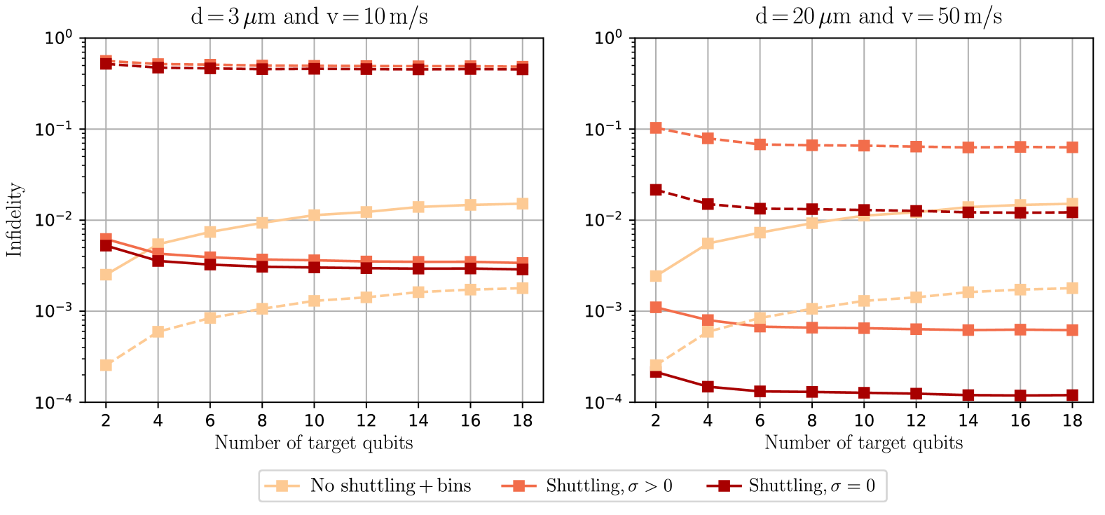
Figure 11: Single-qubit gate infidelity for the 2$\times$N and looped pipeline architectures in the presence of $n_{t}$ target qubits and $n_{n}=n_{t}-2$ non-target qubits. The left and right panels shed lines respectively correspond to a $g$-factor dispersion $\Delta g=10^{-3}g_{0}$ and $10^{-2}g_{0}$. The targets and non-targets are separated by a magnetic field gradient $GB_{0}$. We consider three different strategies for the gate implementation: binning the frequencies without shuttling the qubits (yellow); shuttling the target and non-target qubits so as to reduce the spreading $\sigma$ of their frequencies (orange); and the same as the latter with additional frequency engineering in order to negate any frequency spreading among the target qubits i.e. setting $\sigma=0$ (brown). In the first case, the drive contains multiple tones at resonance with each bin. In the second and third cases however, we send a single tone either approximately or exactly at resonance with the target qubits (owing to $\sigma$ being finite or not).

V Discussion and outlook

In this work, we consider the pressing issue of individual spin qubits control. When qubits are encoded with a single spin trapped in a quantum dot, single-qubit gates are implemented via the use of magnetic fields, which are hard to localise at the qubit scale. Rather, existing research advocated for the use of a global field with multiple driving tones at resonance with the target qubits frequencies, which are variable in essence, due to interface roughness. This generally induces frequency crowding thus unwanted crosstalk that needs to be addressed. In this piece of research, we design an elegant framework to globally control silicon spin qubits with high fidelity.

More specifically, we demonstrate that electron motion can be utilised to homogenise the $g$-factors it experienced. When the motion takes the form of exchange oscillations between a pair of qubits, both electrons $g$-factors become equal to the mean of the original $g$-factors. When the motion is implemented via spin qubit shuttling, all electrons travelling around a looped shuttling track obtain the same new effective $g$-factor equal to the loop mean $g$-factor. These examples make it clear that the above homogenisation method can be utilised to reduce the number of frequencies in the frequency spectrum. In the present paper, we put this observation to use for the implementation of single-qubit gates. While frequency narrowing had already been identified in the past [25], we here explore a new paradigm where it becomes an essential ingredient to the implementation of quantum gates.

The main result of this paper is that when an electron is transferred between multiple locations, a single-qubit gate can simply be implemented by sending a driving tone at resonance with the mean frequency felt by the electron. The quality of the gate is dependent on the transfer rate (exchange coupling, shuttling speed): highest fidelities are achieved when the transfer rate is large compared to the Rabi frequency and the qubits frequency dispersion. Via numerical simulations, we quantify the amount of error generated by such a protocol and obtain promising estimates in the case of transferring a single electron via shuttling. In particular, we demonstrate that when the shuttling distance is large enough, the qubit $g$-factor dispersion rapidly decreases, meaning that the sole knowledge of the device average $g$-factor $g_{0}$ suffices to set the driving frequency. This alleviates the experimental requirements for a spin-qubit-based quantum computer, by removing the need for a constant monitoring and calibration of the detailed $g$-factor landscape. These promising observations led us to extend our analysis first to two-qubit gates, for which we still showed the suitability of our protocol. Then we aimed to to tackle realistic experimental setups: a 2$\times$N array of qubits and the looped pipeline architecture [24]. Even in these more complex contexts, we showed orders of magnitude improvements of the fidelity of single-qubit gates on selected subsets of qubits compared to previous state-of-the-art techniques.

As future work, it would be valuable to generalise our protocol to more general types of qubits and materials. Here, we focused on electron spins in silicon, where the $g$-tensor anisotropy is small. This means that we were able to only consider scalar $g$-factors. More generally, we believe that effects of stronger spin-orbit coupling can be calibrated away as long as they are known a priori.

Additionally, we envision extending our study to more kinds of architectures. One example is the novel Quantum Snakes on a Plane [22], where logical qubits consist of linearised objects than can be shuttled around large loops made of 2$\times$N filaments. We believe that our protocol could greatly facilitate the implementation of single- and two-qubit cases in this paradigm.

Another direction we wish to explore is the inclusion of various physical and experimental limitations. First, this encompasses off-resonant driving, e.g. stemming from the use of finite-bandwidth driving tones. Second, non-adiabatic effects could arise from the abrupt switching-on and off of the driving pulse and exchange coupling. One could further evaluate if these effects can be tamed via known pulse shaping techniques. Finally, noise would inevitably be present in any experimental chip, e.g. charge noise or valley excitations (when shuttling). It would be valuable to run such simulations, which we overlooked for now in order to solely tackle the qubit addressability problem. These would further inform the user about the trade-offs between the use of our schemes and increased noise when qubits are swapped or shuttled.

Appendix A Modelling the g-factor

The $g$-factor of an electron trapped in a quantum dot in silicon is related to the local spin-orbit fields caused by broken symmetries at the interface where dots form and can be linked to surface roughness, and is thus dependent on the precise position of the electron. As there exists no definitive microscopic description for $g$-factor variations [25, 21], we decide to model it with a 1D Ornstein-Uhlenbeck (OU) $g_{int}(x)$ process. The restriction to 1D is motivated by the fact that we will be concerned by moving electrons along linear shuttling tracks. We chose this process as it allows for the modelling of a continuous random process with a certain correlation length, yet remaining relatively easy to simulate. This model should allow us to capture meaningful insights on the impact of the interface on our protocol [54].

The OU process is characterised by its mean $g_{0}$, its standard deviation $\Delta g$ and its correlation length $\lambda$. In silicon, $g_{0}$ approaches 2 and Ref. [55] estimated that $\Delta g$ lies between $10^{-3}$ and $10^{-2}$. We will study both ends of this range in the paper. Here, $\lambda$ represents the correlation length of the interface roughness which largely dictates the values of the $g$-factors. We will set $\lambda=20$ nm. To be more precise, $g_{int}(x)$ is given as the solution of the following stochastic differential equation,

$$dg_{int}(x)=\frac{1}{\lambda}(g_{0}-g_{int}(x))dx+\sqrt{\frac{2dx}{\lambda}}\Delta gdw(x)$$ (10)

where $w$ represents a Wiener process.

Eq.˜10 corresponds to the $g$-factor at each position $x$, but does not yet describe the $g$-factor $g_{i}$ (appearing in Eq.˜1) of an electron at the position $x_{i}$. One must indeed additionally take into account the spatial delocalisation of the electron around its central position $x_{i}$. To do so, the electron $g$-factor should rather be defined as the average of $g_{int}(x)$ weighted by the modulus squared of the wavefunction.

Consider a single quantum dot centred at $x=x_{i}$, the charge wavefunction of an electron trapped in this dot can be modelled as a Gaussian centred on $x_{i}$ such that,

$$|\psi(x,x_{i})|^{2}=\frac{1}{\mathcal{N}}\exp(-\frac{(x-x_{i})^{2}}{2\lambda_{d}^{2}}),$$ (11)

with $\lambda_{d}=7$ nm nm which leads to a realistic size of the electron’s wavefunction of approximately $40$ nm (the electron is in the region $\pm 3\lambda_{d}$ with a probability of $99\%$) and $\mathcal{N}=\int_{\mathbb{R}}|\psi(x,x_{i})|^{2}dx$ is a normalisation constant. For simplicity, we only consider the wavefunction in 1D as we do not expect it to be heavily modified in the other directions whilst the electron is being shuttled. Note however that our scheme works for any model of $g$ as long as it been characterised beforehand. The averaged $g$-factor $g_{i}$ is thus defined by,

$$g_{i}=g(x_{i})\coloneqq\int_{\mathbb{R}}|\psi(x,x_{i})|^{2}g_{int}(x)dx.$$ (12)

In Fig.˜12, we plot one instance of $g_{int}(x)$ and the corresponding evolution of $g_{i}$.

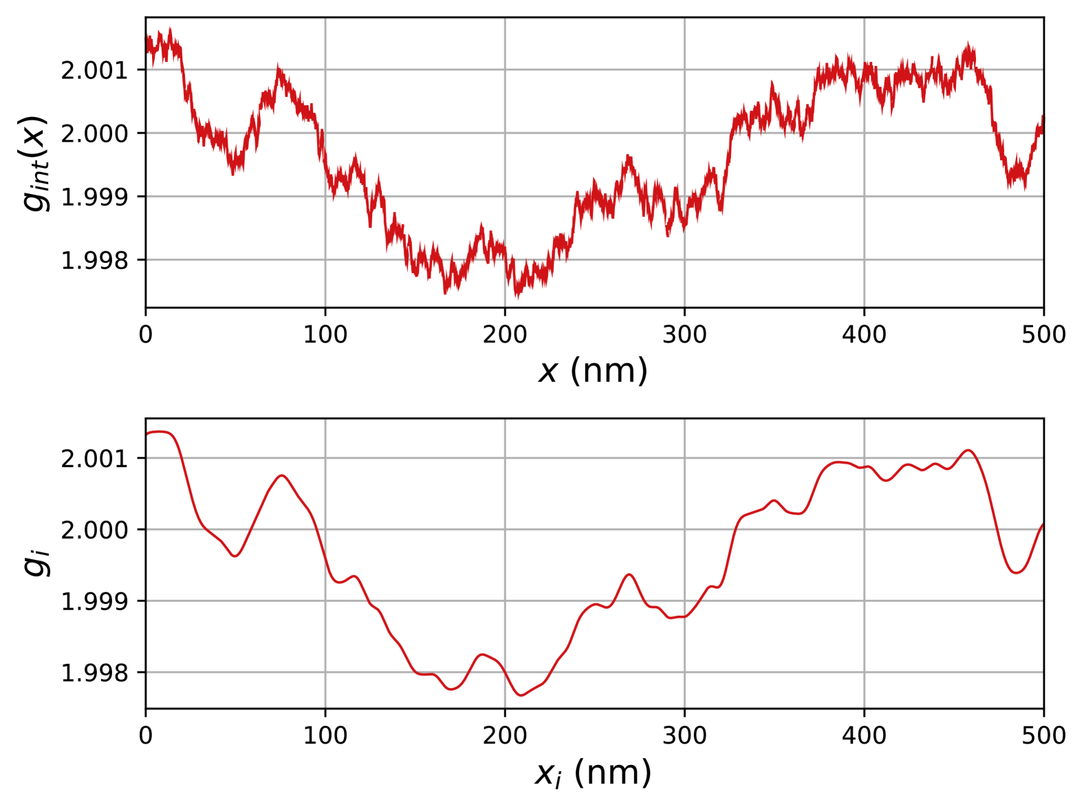
Figure 12: Evolution of one instance of the random $g$-factor $g_{int}(x)$ and the corresponding averaged $g_{i}$. $g_{int}(x)$ is given by a 1D Ornstein-Uhlenbeck process of mean $g_{0}=2$ and standard deviation $\Delta g=10^{-3}$. The averaged $g$-factor is obtained by averaging the position-dependent $g$-factor $g_{int}(x)$ with respect to the electron’s wavefunction $\psi(x,x_{i})$ as in Eq.˜12.

Note that in the main text we dropped the subscript $i$ and used $x$ to denote the position of the centre of the electron’s wavefunction when the context is clear.

Appendix B Impact of using the g-tensor

In Eq.˜1, we use the following Hamiltonian to describe the impact of a magnetic field on the spin of an electron,

$$H_{mag}=g\vec{S}.\vec{B},$$ (13)

where $g$ and $\vec{S}$ represent the $g$-factor and spin of the electron respectively, and $\vec{B}$ the applied global magnetic field. However, as explained in the main text, the most precise way of describing this interaction requires the use of the full $g$-tensor $\mathbb{G}$. In this case, the Hamiltonian is now given by,

$$H_{mag}=\vec{S}^{T}\mathbb{G}\vec{B}.$$ (14)

Simply put, the effect of $\mathbb{G}$ is to change the axes of the applied magnetic field $\vec{B}$, ultimately leading to the modification of our single-qubit gates axes. As this change is position-dependent, this could then hinder our shuttling-based homogenisation protocol presented in Section˜III.2.

Considering a driving field along a single axis and the matrix $\mathbb{G}$ associated to Si/SiO₂ heterostructures, we show here that using the $g$-tensor has minimal impact on the axes of single-qubit rotations. We even show that this impact could be negated, provided perfect knowledge of $\mathbb{G}$. Suppose that $\vec{B}=\vec{B}_{\text{osc}}+\vec{B}_{\text{stat}}$ with $B_{\text{osc}}=(B_{1}\cos(\omega t+\phi),0,0)^{T}$ and $B_{\text{stat}}=(B_{x},B_{y},B_{0})^{T}$ its oscillatory and static parts. While the $z$-component of the Zeeman splitting field is dominant, smaller $x$- and $y$-components can arise due to our use of micromagnets/superconducting lines. Moreover, we will use a matrix $\mathbb{G}$ obtained from atomistic simulations performed by Cifuentes et al. in [35],

$$\mathbb{G}=\begin{pmatrix}g_{0}+\alpha&\beta&g_{13}\\ \beta&g_{0}+\alpha&g_{23}\\ 0&0&g_{33}\end{pmatrix},$$ (15)

where $g_{0}\approx 1.994$, $\alpha\approx-10^{-3}$, $\beta\ \approx\pm 10^{-2}$, $g_{13}\approx\pm 10^{-3}$, $g_{23}\approx\pm 10^{-3}$ and $g_{33}\approx 2.002$ are typical values of the different parameters for Si/SiO₂. We can now expand $H_{mag}$ as follows,

$$H_{mag} =\frac{1}{2}\Big{(}(g_{0}+\alpha)(B_{1}\cos(\omega t+\phi)+B_{x})$$

$$+\beta B_{y}+g_{13}B_{0}\Big{)}\sigma_{x}$$

$$+\frac{1}{2}\Big{(}\beta(B_{1}\cos(\omega t+\phi)+B_{x})$$

$$+(g_{0}+\alpha)B_{y}+g_{23}B_{0}\Big{)}\sigma_{y}$$

$$+\frac{1}{2}g_{33}B_{0}\sigma_{z},$$ (16)

where $\sigma_{x},\sigma_{y}$ and $\sigma_{z}$ are Pauli operators acting on the spin degree of freedom.

To simplify our study, we now consider $H_{mag}$ in a frame rotating at the drive frequency $\omega$ by performing the following transformation,

$$H_{mag}(t) \rightarrow H_{mag}^{{}^{\prime}}(t)=U(t)H_{mag}(t)U^{\dagger}(t)+i\frac{dU}{dt}(t)U^{\dagger}(t),$$ (17)

with

$$U(t)=\exp(i\frac{\omega}{2}\sigma_{z}t).$$ (18)

Using the rotating-wave approximation we get,

$$H_{mag}^{{}^{\prime}} =\frac{1}{4}g_{0}\tilde{B}_{1}\cos(\theta+\phi)\sigma_{x}$$

$$+\frac{1}{4}g_{0}\tilde{B}_{1}\sin(\theta+\phi)\sigma_{y}$$

$$+\frac{1}{2}(g_{33}B_{0}-\omega)\sigma_{z},$$ (19)

where $\cos(\theta)=(1+(\beta/(g_{0}+\alpha))^{2})^{-1/2}$ and $\tilde{B}_{1}=\sqrt{(1+\alpha/g_{0})^{2}+(\beta/g_{0})^{2}}B_{1}$.

More precisely, supposing that $\phi=0$, instead of obtaining a rotation along the $x$-axis with Rabi frequency $g_{0}B_{1}$ (as expected from the Rabi model), the use of the $g$-tensor leads to a rotation along the axis $(\cos(\theta),\sin(\theta),0)^{T}$ with a slightly modified frequency $g_{0}\tilde{B}_{1}$. Using the values extracted from [35], we find that $\sin(\theta)\approx O(10^{-3})$ and $|B_{1}-\tilde{B}_{1}|/B_{1}\approx O(10^{-4})$, which has a negligible impact on the gate fidelity. Finally, we can approximate $H^{{}^{\prime}}_{mag}$ by,

$$H^{{}^{\prime}}_{mag}\approx\frac{1}{4}g_{0}B_{1}\sigma_{x}+\frac{1}{2}(g_{33}B_{0}-\omega)\sigma_{z}.$$ (20)

which validates our assumption that the oscillatory and static fields are respectively applied along the $x$ and $z$ axes. For commodity we will additionally assume that $g_{0}\approx g_{33}$, which allows us to consider a scalar $g$-factor.

Alternatively, if we have perfect knowledge of $\mathbb{G}$, we can control the rotation axis and obtain a perfect rotation around the $x$-axis by setting $\phi=-\theta$. The rotation frequency $\tilde{B}_{1}$ would also be fully characterised.

Appendix C Numerical simulations

To quantify the success of each technique we present in this paper, we measure the fidelity of the implemented operation via the matrix norm:

$$\mathcal{F}=\frac{1}{4}\left|\mathrm{Tr}(U_{\text{target}}^{\dagger}\tilde{U})\right|^{2/n_{q}}$$ (21)

where $U_{\text{target}}=X^{\otimes n_{t}}\otimes I^{\otimes n_{q}-n_{t}}$ is the target unitary and $\tilde{U}$ is a slightly modified version of the time evolution operator $U$ as explained in Eq.˜24. Note that this expression is an average single-qubit fidelity over the $n_{q}$ qubits, which is why an $n_{q}$-th root is taken. As $H$ is time-dependent, we compute $U$ by discretisation of the time, with time step $dt=T/N_{\text{steps}}$, where $T=\pi/\Omega$ is the total gate time of an $X$ gate with drive strength $\Omega$. $N_{\text{steps}}$ is set to $10,000$, such that the simulations converge.

When the qubits are non-interacting and as this time discretisation induces a computational overhead, we simplify the calculations by further decomposing the fidelity $\mathcal{F}$ into a product of single-qubit fidelities. These single-qubit fidelities are then slightly modified, by noting that known but unwanted $Z$-rotations can easily be cancelled out by a change of rotating frame (or equivalently via the implementation of a virtual $Z$ gate) [56]. Therefore, when evaluating the success of a single-qubit gate, one should remove the $Z$ components of the implemented unitary $U$.

A general representation of any $SU(2)$ gate is:

$$U =\begin{pmatrix}\mathrm{cos}(\theta/2)&-i\mathrm{e}^{i\lambda}\mathrm{sin}(\theta/2)\\ -i\mathrm{e}^{i\phi}\mathrm{sin}(\theta/2)&\mathrm{e}^{i(\lambda+\phi)}\mathrm{cos}(\theta/2)\\ \end{pmatrix}$$ (22)

$$=Z_{\phi}X_{\theta}Z_{\lambda}$$ (23)

with $P_{\alpha}=\mathrm{e}^{-i\alpha P/2}$ and $X$ and $Z$ the Pauli operators. Removing the $Z$-rotations from $U$ thus amounts to setting $\phi=\lambda=0$. As $\theta\in[0,\pi[$, this is equivalent to considering the modified time-evolution operator

$$\tilde{U}=\begin{pmatrix}|u_{0,0}|&-i|u_{0,1}|\\ -i|u_{1,0}|&|u_{1,1}|\end{pmatrix}$$ (24)

with $u_{i,j}$ the coefficients of the matrix $U$.

The case of two-qubit gates (for the exchange-coupling scheme) is more complex and was not implemented here, which means that we will not attempt in this case to remove unwanted $Z$ rotations.

Finally, note that we will only study unitary evolutions in this paper, thus not simulating noise processes such as charge noise or shuttling noise. If we were to include them in our simulations, the resulting infidelities would only saturate at a level given by the strength of the dominant noise source.

Appendix D Residual entanglement in the exchange-based homogenisation

In an attempt to better understand the unitary operation $U$ resulting in the simultaneous driving and swapping, we decided to extend our study to its Schmidt decomposition. Mathematically, any vector in the tensor product of two vector spaces can be expressed as a sum of tensor products. Applied to $U$, this reads:

$$U=\sum_{i=1}^{m}\alpha_{i}V_{i}\otimes W_{i}$$ (25)

where for all $i\in\llbracket 1,m\rrbracket$, $V_{i}$ and $W_{i}$ are single-qubit unitary operations on the first and second qubit respectively, and $\alpha_{i}\in\mathbb{C}$. This decomposition is thus a very convenient way to deduce if a two-qubit unitary is a product of two single-qubit unitaries, in which case only one $\alpha_{i}$ should be non-zero. In our setup, we verified that the ideal case of instantaneous swapping led to a single non-vanishing $\alpha_{i}$ with the expected unitaries: two single-qubit rotations around the $x$-axis at frequency $\Omega$. We then aimed to understand if beyond this ideal case, the resulting unitary $U$ could be written as the product of two single-qubit rotations, potentially around slightly off axes or with slightly different Rabi frequencies. We however found that reducing the ratios $J/\Omega$ or $\Omega/\omega_{q}^{12}$ inevitably led, even to first order, to more than one non-vanishing $\alpha_{i}$. Finite values of such ratios thus necessarily, but also quite expectedly, increase the entanglement power of the operation. This results in an unwanted mixing of the single-qubit states, that seems to be the first source of infidelity: the only solution against this thus is to operate with higher values of the above ratios. The easiest way to do so is to increase the exchange coupling $J$. However, it might be experimentally challenging to operate with large exchange couplings.

Appendix E Tunnel-coupling-based homogenisation

E.1 Hamiltonian

When studying a single electron in a DQD, one needs to take into account the charge degree of freedom which is not explicitly apparent in Eq.˜1. The homogenisation induced by the usage of the tunnel coupling is based on the fact that the left and right dots have different frequencies $\omega_{q,1}$ and $\omega_{q,2}$ respectively and that the charge of the electron will oscillate between the two when the barrier is lowered.

The Hamiltonian in the laboratory frame of reference is given by:

$$H_{single} =\frac{\omega_{q,1}}{2}\outerproduct{\text{L}}{\text{L}}\otimes\sigma_{z}+\frac{\omega_{q,2}}{2}\outerproduct{\text{R}}{\text{R}}\otimes\sigma_{z}$$

$$+\varepsilon\tau_{z}\otimes I+t_{c}\tau_{x}\otimes I$$

$$+\Omega\cos(\omega t+\phi)I\otimes\sigma_{x},$$ (26)

where $\varepsilon$ is the DQD detuning, $\tau_{x}=\outerproduct{\text{L}}{\text{R}}+\outerproduct{\text{R}}{\text{L}}$, $\tau_{z}=\outerproduct{\text{L}}{\text{L}}-\outerproduct{\text{R}}{\text{R}}$, $\{\sigma_{i}\}_{x,z}$ the Pauli operators acting on the charge and spin degrees of freedom respectively and $\Omega,\omega,\phi$ the drive amplitude, frequency and phase. Here, we set $\varepsilon=0$ as one would do in an experiment in order to be first-order insensitive to charge noise, and $\phi=0$ as we want to perform an X gate.

By lowering the barrier between the dots, the electron will start oscillating (with a frequency $t_{c}$) between the charge states of the two dots $\ket{\text{L}}$ and $\ket{\text{R}}$ with frequencies $\omega_{q,1}$ and $\omega_{q,2}$ respectively (see Fig.˜13). As in Section˜III, we expect that sending a drive at the average frequency $\bar{\omega}_{q}=(\omega_{q,1}+\omega_{q,2})/2$ should result in an $X$ gate. Note that for the qubit to come back to its initial position at the end of the gate, the following condition must be satisfied,

$$t_{c}=2p\Omega,~~p\in\mathbb{N}$$ (27)

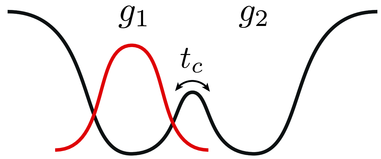
Figure 13: Tunnel-coupling based homogenisation. We consider two dots with different $g$-factor. As explained in Section˜III, increasing the transfer rate $t_{c}$ allows an electron to acquire an effective $g$-factor equal to the average of that of the two dots. While this method does not allow for the reduction of the number of frequencies, it allows for a greater tunability as explained in Section˜E.3.

E.2 Numerical simulation

In order to characterise the quality of our protocol, we plot the evolution of the fidelity (as defined in Appendix˜C) between the implemented unitary $U$ and the target unitary $U_{\text{target}}$ for different values of the ratios $\omega_{q}^{12}/\Omega$ and $t_{c}/\Omega$ in Fig.˜14. Note that the Hamiltonian used here is different from the one defined in Eq.˜1 as explained in Section˜E.1. Similarly as in Fig.˜4 the infidelity naturally drops as the transfer rate increases and as $\omega_{q}^{12}$ decreases. Moreover, as the compute time for large $t_{c}$ was forbiddingly high, we obtain the last data point by linear extrapolation (dashed lines). Using values from Table˜1, i.e. $t_{c}/\Omega=10^{4}$ and $\omega_{q}^{12}/\Omega\gtrsim 1$, we obtain an infidelity between $10^{-7}$ and $10^{-8}$. Note that such low values will in practice be capped by other sources of noise (e.g. charge noise). Therefore this only means that the errors induced by our protocol will not be a limiting factor.

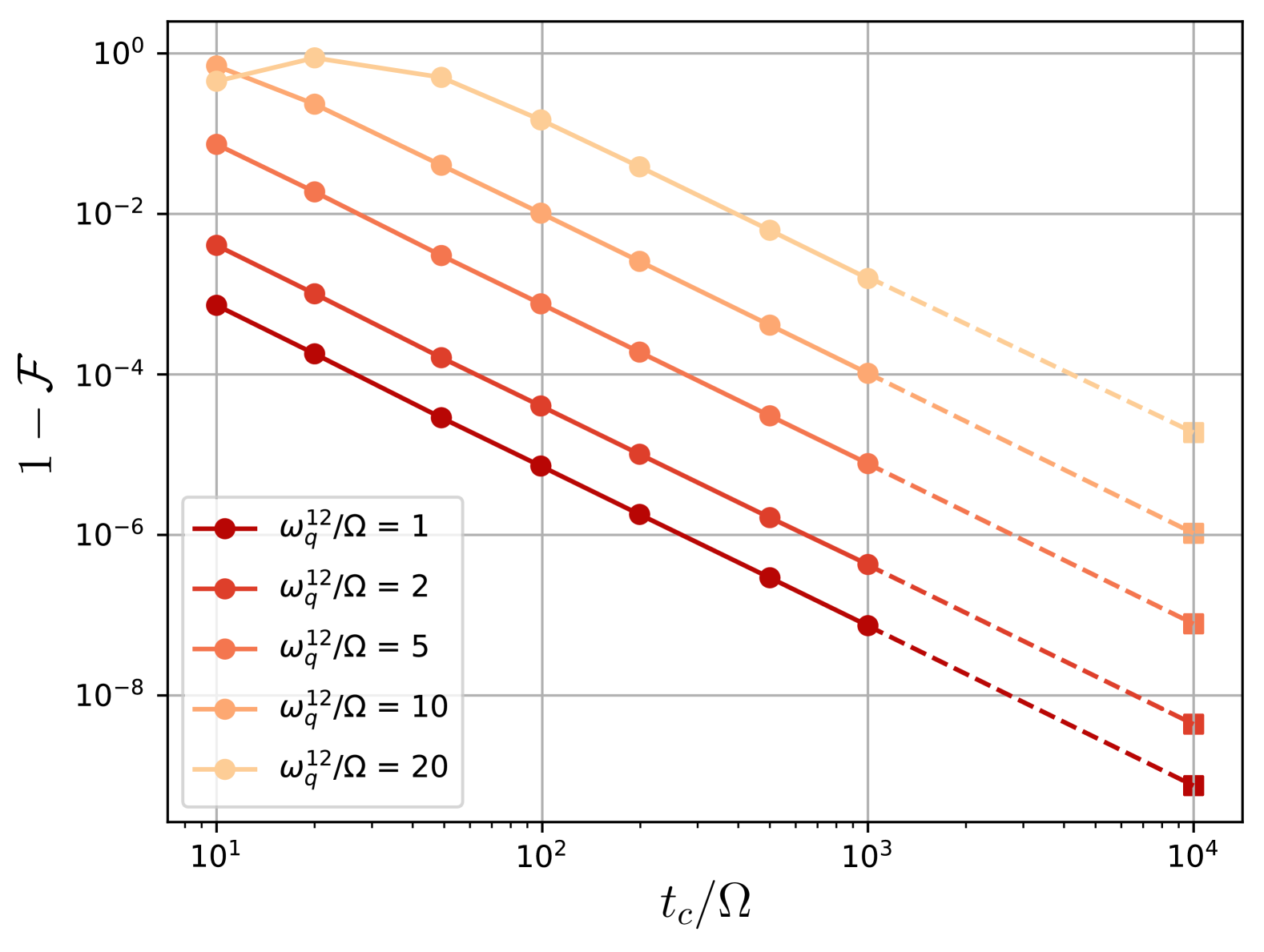
Figure 14: Infidelity of the tunnel-coupling based protocol. It is computed as the infidelity of implementing an $X$ gate when driving a qubit oscillating between two quantum dots with frequencies $\omega_{q,1}$ and $\omega_{q,2}$ respectively with a single driving tone at $\omega=\bar{\omega}_{q}$. The data is plotted against $t_{c}/\Omega$ and $\omega_{q}^{12}/\Omega$, where $t_{c}$ is the tunnel coupling and $\omega_{q}^{12}=\omega_{q,2}-\omega_{q,1}$. $t_{c}$ is always chosen such that the condition in Eq.˜27 is satisfied. The dashed lines extend the data to $t_{c}/\Omega=10^{4}$ which corresponds to practical values of $t_{c}$. The squares corresponds to the extrapolated values of the infidelity.

While this technique benefits from larger transfer rates and thus lower infidelities, it does not allow for a reduction of the number of distinct frequencies in the spectrum. Moreover, it requires an extra empty dot to be placed near every qubit, which is not practical as the device scales. However, it allows for a larger tunability of the $g$-factors compared to that offered by the Stark shift as explained in the next section. Such increased tunability could be leveraged when needed, in order to increase the distance between qubit frequencies and thus reduce crosstalk.

E.3 Increased tunability

Contrary to the other methods, we do not reduce the number of distinct frequencies in the spectrum by using the tunnel coupling. However, we can still increase the tunability of the $g$-factors and thus reduce crosstalk by increasing the distance between frequencies. Consider a single electron trapped in the left dot of a double quantum dot, such that its frequency is equal to $\omega_{q,1}$. In practice, the average difference in frequencies between the dots is approximately equal to $\omega_{q}^{12}=\Delta\omega_{q}=\Delta gB_{0}$, with $\Delta g$ the standard deviation of the $g$-factor as defined in Eq.˜10. By lowering the barrier, we showed previously that the electron obtains an average frequency equal to $\bar{\omega}_{q}=(\omega_{q,1}+\omega_{q,2})/2$. This means that we managed to tune the frequency by an amount $\bar{\omega}_{q}-\omega_{q,1}=\Delta\omega_{q}/2$. Usually, the frequency of an electron can be tuned using the Stark shift by an amount $\delta\omega_{q}=0.1\Delta\omega_{q}<\Delta\omega_{q}/2$.

Appendix F Crosstalk suppression via synchronisation

In all the applications we present in Section˜IV, we send driving pulses targetting a subset of the qubits, and wish to minimise the impact of each pulse on the qubits it does not target. This is in general enforced by maximising the spacing between drives and non-targetted qubits (thereby minimising off-resonant effects). Here we show that additionally tuning the drive strength $\Omega$ can help further mitigate these crosstalk effects. Namely, a clever choice of $\Omega$ can allow for the synchronisation of the oscillations of the electrons, such that the non-target qubits perform a $2\pi$ rotation (identity gate) while the target qubits perform a $\pi$ rotation ($X$ gate).

Let us first focus on the case where only one target frequency and one non-target frequency are present in the frequency spectrum. This essentially describes all our shuttling-based applications from Section˜IV (although in general there subsists a small dispersion $\sigma$ around these main frequencies). In this case, one can equate the times taken by one $X$ gate on the target qubits and a $2p\pi$ ($p\in\mathbb{N}$) rotation of the non-target qubits by enforcing the condition,

$$\frac{\pi}{\Omega}=\frac{2p\pi}{\sqrt{\Omega^{2}+(\omega_{q}^{12})^{2}}},$$ (28)

with $(\omega_{q}^{12})^{2}$ the difference between the effective target and non-target frequencies. The target qubits theoretically oscillate at a frequency $\Omega$, while off-resonant effects induce oscillations of the non-target qubits at frequency $\sqrt{\Omega^{2}+(\omega_{q}^{12})^{2}}$ as inferred from the Rabi model. This results in setting:

$$\Omega=\frac{\omega_{q}^{12}}{\sqrt{4p^{2}-1}},~~p\in\mathbb{N}$$ (29)

By reducing the spectrum to only one target and one non-target frequencies, setting the above condition totally removes any crosstalk infidelity as non-target qubits exactly perform an identity gate while target qubits perform an $X$ rotation.

When using the binning scheme, it is in general not possible to reduce the frequency spectrum to only two frequencies. In this case, we can generalise the above condition as follows (Section B of [14] with a bin width $2\delta\omega_{q}$):

$$\Omega=\frac{\delta\omega_{q}}{p},~~p\in\mathbb{N}$$ (30)

where $p$ is a free parameter that can be adjusted according to the achievable values of $\Omega$ and $\delta\omega_{q}$. This is a generalisation of Eq.˜29, where the existence of only two frequencies in the frequency spectrum permitted the complete removal of crosstalk effects. Here the extension to more than two frequencies only allows for a partial reduction of the crosstalk.

Note that in both cases $\Omega\leq\omega_{q}^{12}$, meaning that if the frequencies are close to each other, slower gates will be obtained.

Appendix G Estimation of the right parameter regime

G.1 Shuttling-based scheme

In Section˜IV.1, we stated the values of experimental parameters which a posteriori led to a high performance of our shuttling-based protocol. In this section, we further justify this choice with some analytical arguments.

Firstly, our shuttling-based homogenisation performs best at low frequency dispersion, justifying to work in the regime $\Delta g=10^{-3}g_{0}$ and $B_{0}=0.1$ T. Second, the dispersion of target frequencies around the driving frequency (due to finite $\sigma$) means that target qubits are not exactly driven at resonance. This undesired effect is minimised at large $\Omega$, which is also synonym of faster gates. This is also observed in the second panel of Fig.˜6. For this reason, we set $\Omega=5$ MHz.

Let us now evaluate the target values of the last key experimental parameters enabling the full power of our protocol i.e. the required $g$-factor shift $G$, the shuttling length $d$ and the shuttling speed $v$. We will first focus on the case of a constant applied frequency shift $GB_{0}$ between the targets and non-targets. In this case $\sigma>0$. We will estimate these parameters by distinguishing two main contributions to the infidelity: the slightly off-resonant driving of the homogenised data qubits and the crosstalk with the non-target qubits. We wish to bring each of these contributions below $2\times 10^{-3}$ for at least $95\%$ of the qubits, so as to be comfortably below the surface code threshold. If the locations of the $5\%$ outliers are known, the error they generate can be mitigated by suitable QEC protocols as erasure errors [57].

The first contribution reads:

$$I_{1}=\frac{1}{1+\left(\frac{\Omega}{2\sigma B_{0}}\right)^{2}}$$ (31)

from the Rabi model, where we use $2\sigma B_{0}$ for the frequency mismatch between the drive and a given target qubit so as to cover $95\%$ of the qubits. $\sigma$ is the standard deviation of the homogenised $g$-factors

$$\bar{g}=\frac{1}{d}\int_{0}^{d}g(x)\mathrm{d}x.$$ (32)

In a first approximation, we can write

$$\sigma=\frac{\Delta g}{\sqrt{d/\lambda}}$$ (33)

where $\lambda$ is the coherence length of the $g$-factor landscape. This equation simply states that the standard deviation of the average of independent random variables decreases as $1/\sqrt{N}$, where $N$ is the number of samples. This leads to:

$$I_{1}=\frac{1}{1+\frac{\Omega^{2}}{4\Delta\omega_{q}^{2}}\frac{d}{\lambda}}$$ (34)

with $\Delta\omega_{q}=\Delta gB_{0}$. By setting $I_{1}=2\times 10^{-3}$ we find a minimum shuttling distance $d\geq 14\;\mu$m. From this we can deduce the minimum shuttling speed enabling the exploration of such a distance during the gate time $T=\pi/\Omega$:

$$v=\frac{\Omega d}{\pi}$$ (35)

We deduce $v\geq 23\text{ m/s}$. We can now evaluate the infidelity arising from the crosstalk with non-target qubits:

$$I_{2}=\frac{1}{1+\left(\frac{GB_{0}}{\Omega}\right)^{2}}$$ (36)

We here neglect the dispersion $\sigma$ of the non-target qubits around their mean $g$-factor as it is negligible compared to $G$. We here find $G\geq 160$ MHz. Note that for simplicity, we do not describe here the crosstalk reductions offered by the technique of Appendix˜F. This would permit for lower values of $G$.

In the case where the magnetic field gradient can be tuned so as to annihilate the frequency dispersion $\sigma$, the infidelity is only limited by the performance of our homogenisation protocol (which we neglected in the previous case). Indeed, $I_{1}$ vanishes as $\sigma=0$ (all targets are resonantly driven) and $I_{2}$ as well as Eq.˜29 guarantees a total suppression of the crosstalk in the strict presence of two frequencies in the spectrum. Therefore, $G$ can be chosen arbitrarily, as long as $GB_{0}\geq$ 5 MHz (remember that Eq.˜29 enforces $\Omega\leq GB_{0}$). As for $v$ and $d$, their values can be inferred from the top panel of Fig.˜6, which describes a driving at exact resonance with the homogenised target frequency. At $\Omega=5$ MHz, the resulting infidelity (from imperfect homogenisation) never exceeds $0.4\%$, meaning no value of $d$ and no value of $v\leq 10$m/s would be an impediment to surface-code-enabled error correction.

Note however that these models are highly simplified for the ease of parameter estimation, using worst-case approximations. Consequently, although the first parameter regime we considered in Section˜IV (left panel of Fig.˜11) does not rigorously respect the conditions we here set, it still yields desirable performances.

G.2 Binning scheme

We proceed similarly for the binning scheme. Its performance is maximised at large interbin spacing, which is given by $2\delta\omega_{q}=2\Delta gB_{0}/10$. It thus optimal to work at higher interface roughness and higher magnetic field in this case: $\Delta g=10^{-2}g_{0}$ and $B_{0}=1$ T. Another reason for this choice is that enforcing Eq.˜30 for crosstalk reduction (which is crucial here) implies $\Omega\leq\delta\omega_{q}$. $\delta\omega_{q}$ must therefore be kept relatively high to ensure that gates are fast. With the above choice of parameters, we obtain $\delta\omega_{q}=30$ MHz, which would not be a bottleneck. Besides, the previous analysis leading to $G\geq 160$ MHz is still valid here.

G.3 Hybrid shuttling-binning scheme

We briefly mention here that one further protocol we envisioned was to combine the shuttling and binning schemes. Once qubits are shuttled, rather than targetting them at a mean slightly off-resonant frequency $\omega=GB_{0}$, one could envisage to place the post-shuttling effective frequencies into bins and resonantly target them with multiple driving tones. While this two-step frequency factorisation protocol sounds powerful on paper, it would not lead to desirable fidelities as the shuttling and binning schemes are not operated in the same parameter regime (they respectively work best at low and high $\Delta\omega_{q}$).

References

- Mills et al. [2022] A. R. Mills, C. R. Guinn, M. J. Gullans, A. J. Sigillito, M. M. Feldman, E. Nielsen, and J. R. Petta, Two-qubit silicon quantum processor with operation fidelity exceeding 99%, Science Advances 8, eabn5130 (2022).
- Noiri et al. [2022] A. Noiri, K. Takeda, T. Nakajima, T. Kobayashi, A. Sammak, G. Scappucci, and S. Tarucha, Fast universal quantum gate above the fault-tolerance threshold in silicon, Nature 601, 338 (2022).
- Xue et al. [2022] X. Xue, M. Russ, N. Samkharadze, B. Undseth, A. Sammak, G. Scappucci, and L. M. K. Vandersypen, Quantum logic with spin qubits crossing the surface code threshold, Nature 601, 343 (2022).
- Stano and Loss [2022] P. Stano and D. Loss, Review of performance metrics of spin qubits in gated semiconducting nanostructures, Nature Reviews Physics 4, 672–688 (2022).
- Maurand et al. [2016] R. Maurand, X. Jehl, D. Kotekar-Patil, A. Corna, H. Bohuslavskyi, R. Laviéville, L. Hutin, S. Barraud, M. Vinet, M. Sanquer, and S. De Franceschi, A CMOS silicon spin qubit, Nature Communications 7, 13575 EP (2016).
- Gonzalez-Zalba et al. [2021] M. F. Gonzalez-Zalba, S. de Franceschi, E. Charbon, T. Meunier, M. Vinet, and A. S. Dzurak, Scaling silicon-based quantum computing using CMOS technology, Nature Electronics 4, 872 (2021).
- Zwerver et al. [2022] A. M. J. Zwerver, T. Krähenmann, T. F. Watson, L. Lampert, H. C. George, R. Pillarisetty, S. A. Bojarski, P. Amin, S. V. Amitonov, J. M. Boter, R. Caudillo, D. Correas-Serrano, J. P. Dehollain, G. Droulers, E. M. Henry, R. Kotlyar, M. Lodari, F. Lüthi, D. J. Michalak, B. K. Mueller, S. Neyens, J. Roberts, N. Samkharadze, G. Zheng, O. K. Zietz, G. Scappucci, M. Veldhorst, L. M. K. Vandersypen, and J. S. Clarke, Qubits made by advanced semiconductor manufacturing, Nature Electronics 5, 184 (2022).
- Chittock-Wood et al. [2024] J. F. Chittock-Wood, R. C. C. Leon, M. A. Fogarty, T. Murphy, S. M. Patomäki, G. A. Oakes, F.-E. von Horstig, N. Johnson, J. Jussot, S. Kubicek, B. Govoreanu, D. F. Wise, M. F. Gonzalez-Zalba, and J. J. L. Morton, Exchange control in a mos double quantum dot made using a 300 mm wafer process (2024), arXiv:2408.01241 [cond-mat.mes-hall] .
- Steinacker et al. [2024] P. Steinacker, N. D. Stuyck, W. H. Lim, T. Tanttu, M. Feng, A. Nickl, S. Serrano, M. Candido, J. D. Cifuentes, F. E. Hudson, K. W. Chan, S. Kubicek, J. Jussot, Y. Canvel, S. Beyne, Y. Shimura, R. Loo, C. Godfrin, B. Raes, S. Baudot, D. Wan, A. Laucht, C. H. Yang, A. Saraiva, C. C. Escott, K. D. Greve, and A. S. Dzurak, A 300 mm foundry silicon spin qubit unit cell exceeding 99in all operations (2024), arXiv:2410.15590 [cond-mat.mes-hall] .
- George et al. [2025] H. C. George, M. T. Mądzik, E. M. Henry, A. J. Wagner, M. M. Islam, F. Borjans, E. J. Connors, J. Corrigan, M. Curry, M. K. Harper, D. Keith, L. Lampert, F. Luthi, F. A. Mohiyaddin, S. Murcia, R. Nair, R. Nahm, A. Nethwewala, S. Neyens, B. Patra, R. D. Raharjo, C. Rogan, R. Savytskyy, T. F. Watson, J. Ziegler, O. K. Zietz, S. Pellerano, R. Pillarisetty, N. C. Bishop, S. A. Bojarski, J. Roberts, and J. S. Clarke, 12-spin-qubit arrays fabricated on a 300 mm semiconductor manufacturing line, Nano Letters 25, 793 (2025).
- Kane [1998] B. E. Kane, A silicon-based nuclear spin quantum computer, Nature 393, 133 (1998).
- Vahapoglu et al. [2021] E. Vahapoglu, J. P. Slack-Smith, R. C. C. Leon, W. H. Lim, F. E. Hudson, T. Day, T. Tanttu, C. H. Yang, A. Laucht, A. S. Dzurak, and J. J. Pla, Single-electron spin resonance in a nanoelectronic device using a global field, Science Advances 7, eabg9158 (2021).
- Hansen et al. [2024] I. Hansen, A. E. Seedhouse, S. Serrano, A. Nickl, M. Feng, J. Y. Huang, T. Tanttu, N. Dumoulin Stuyck, W. H. Lim, F. E. Hudson, K. M. Itoh, A. Saraiva, A. Laucht, A. S. Dzurak, and C. H. Yang, Entangling gates on degenerate spin qubits dressed by a global field, Nature Communications 15, 10.1038/s41467-024-52010-4 (2024).
- Fayyaz and Kestner [2023] A. Fayyaz and J. P. Kestner, Enhanced local addressability of a spin array with local exchange pulses and global microwave driving, Physical Review B 108, 10.1103/physrevb.108.l081303 (2023).
- Veldhorst et al. [2015] M. Veldhorst, R. Ruskov, C. H. Yang, J. C. C. Hwang, F. E. Hudson, M. E. Flatté, C. Tahan, K. M. Itoh, A. Morello, and A. S. Dzurak, Spin-orbit coupling and operation of multivalley spin qubits, Phys. Rev. B 92, 201401 (2015).
- Huang et al. [2017] W. Huang, M. Veldhorst, N. M. Zimmerman, A. S. Dzurak, and D. Culcer, Electrically driven spin qubit based on valley mixing, Phys. Rev. B 95, 075403 (2017).
- Ferdous et al. [2018a] R. Ferdous, E. Kawakami, P. Scarlino, M. P. Nowak, D. R. Ward, D. E. Savage, M. G. Lagally, S. N. Coppersmith, M. Friesen, M. A. Eriksson, L. M. K. Vandersypen, and R. Rahman, Valley dependent anisotropic spin splitting in silicon quantum dots, npj Quantum Information 4, 26 (2018a).
- Tanttu et al. [2019] T. Tanttu, B. Hensen, K. W. Chan, C. H. Yang, W. W. Huang, M. Fogarty, F. Hudson, K. Itoh, D. Culcer, A. Laucht, A. Morello, and A. Dzurak, Controlling spin-orbit interactions in silicon quantum dots using magnetic field direction, Phys. Rev. X 9, 021028 (2019).
- Patomäki et al. [2023] S. M. Patomäki, M. F. Gonzalez-Zalba, M. A. Fogarty, Z. Cai, S. C. Benjamin, and J. J. L. Morton, Pipeline quantum processor architecture for silicon spin qubits (2023), arXiv:2306.07673 [quant-ph] .
- Xue et al. [2024] R. Xue, M. Beer, I. Seidler, S. Humpohl, J.-S. Tu, S. Trellenkamp, T. Struck, H. Bluhm, and L. R. Schreiber, Si/SiGe QuBus for single electron information-processing devices with memory and micron-scale connectivity function, Nature Communications 15, 2296 (2024).
- Siegel et al. [2024] A. Siegel, A. Strikis, and M. Fogarty, Towards early fault tolerance on a array of qubits equipped with shuttling, PRX Quantum 5, 040328 (2024).
- Siegel et al. [2025] A. Siegel, Z. Cai, H. Jnane, B. Koczor, S. Pexton, A. Strikis, and S. Benjamin, Snakes on a plane: mobile, low dimensional logical qubits on a 2d surface (2025), arXiv:2501.02120 [quant-ph] .
- Li et al. [2018] R. Li, L. Petit, D. P. Franke, J. P. Dehollain, J. Helsen, M. Steudtner, N. K. Thomas, Z. R. Yoscovits, K. J. Singh, S. Wehner, L. M. K. Vandersypen, J. S. Clarke, and M. Veldhorst, A crossbar network for silicon quantum dot qubits, Science Advances 4, eaar3960 (2018), https://www.science.org/doi/pdf/10.1126/sciadv.aar3960 .
- Cai et al. [2023] Z. Cai, A. Siegel, and S. Benjamin, Looped pipelines enabling effective 3d qubit lattices in a strictly 2d device, PRX Quantum 4, 10.1103/prxquantum.4.020345 (2023).
- Langrock et al. [2023] V. Langrock, J. A. Krzywda, N. Focke, I. Seidler, L. R. Schreiber, and L. Cywiński, Blueprint of a scalable spin qubit shuttle device for coherent mid-range qubit transfer in disordered si/sige/sio 2, PRX Quantum 4, 10.1103/prxquantum.4.020305 (2023).
- Micciche et al. [2025] A. Micciche, A. Chatterjee, A. McGregor, and S. Krastanov, Optimizing compilation of error correction codes for 2xn quantum dot arrays and its np-hardness (2025), arXiv:2501.09061 [quant-ph] .
- Shehata et al. [2023] M. M. E. K. Shehata, G. Simion, R. Li, F. A. Mohiyaddin, D. Wan, M. Mongillo, B. Govoreanu, I. Radu, K. De Greve, and P. Van Dorpe, Modeling semiconductor spin qubits and their charge noise environment for quantum gate fidelity estimation, Phys. Rev. B 108, 045305 (2023).
- Cifuentes et al. [2023] J. D. Cifuentes, P. Y. Mai, F. Schlattner, H. E. Ercan, M. Feng, C. C. Escott, A. S. Dzurak, and A. Saraiva, Path-integral simulation of exchange interactions in cmos spin qubits, Phys. Rev. B 108, 155413 (2023).
- Jnane and Benjamin [2024] H. Jnane and S. C. Benjamin, Ab initio modelling of quantum dot qubits: Coupling, gate dynamics and robustness versus charge noise (2024), arXiv:2403.00191 [cond-mat.mes-hall] .
- Yoneda et al. [2018] J. Yoneda, K. Takeda, T. Otsuka, T. Nakajima, M. R. Delbecq, G. Allison, T. Honda, T. Kodera, S. Oda, Y. Hoshi, N. Usami, K. M. Itoh, and S. Tarucha, A quantum-dot spin qubit with coherence limited by charge noise and fidelity higher than 99.9%, Nature Nanotechnology 13, 102 (2018).
- Yang et al. [2019] C. H. Yang, K. W. Chan, R. Harper, W. Huang, T. Evans, J. C. C. Hwang, B. Hensen, A. Laucht, T. Tanttu, F. E. Hudson, S. T. Flammia, K. M. Itoh, A. Morello, S. D. Bartlett, and A. S. Dzurak, Silicon qubit fidelities approaching incoherent noise limits via pulse engineering, Nature Electronics 2, 151–158 (2019).
- Yoneda et al. [2021] J. Yoneda, W. Huang, M. Feng, C. H. Yang, K. W. Chan, T. Tanttu, W. Gilbert, R. C. C. Leon, F. E. Hudson, K. M. Itoh, A. Morello, S. D. Bartlett, A. Laucht, A. Saraiva, and A. S. Dzurak, Coherent spin qubit transport in silicon, Nature Communications 12, 10.1038/s41467-021-24371-7 (2021).
- Seidler et al. [2022] I. Seidler, T. Struck, R. Xue, N. Focke, S. Trellenkamp, H. Bluhm, and L. R. Schreiber, Conveyor-mode single-electron shuttling in si/sige for a scalable quantum computing architecture, npj Quantum Information 8, 10.1038/s41534-022-00615-2 (2022).
- Smet et al. [2024] M. D. Smet, Y. Matsumoto, A.-M. J. Zwerver, L. Tryputen, S. L. de Snoo, S. V. Amitonov, A. Sammak, N. Samkharadze, Önder Gül, R. N. M. Wasserman, M. Rimbach-Russ, G. Scappucci, and L. M. K. Vandersypen, High-fidelity single-spin shuttling in silicon (2024), arXiv:2406.07267 [cond-mat.mes-hall] .
- Cifuentes et al. [2024] J. D. Cifuentes, T. Tanttu, W. Gilbert, J. Y. Huang, E. Vahapoglu, R. C. C. Leon, S. Serrano, D. Otter, D. Dunmore, P. Y. Mai, F. Schlattner, M. Feng, K. Itoh, N. Abrosimov, H.-J. Pohl, M. Thewalt, A. Laucht, C. H. Yang, C. C. Escott, W. H. Lim, F. E. Hudson, R. Rahman, A. S. Dzurak, and A. Saraiva, Bounds to electron spin qubit variability for scalable CMOS architectures, Nature Communications 15, 4299 (2024).
- Wang et al. [2024] C.-A. Wang, V. John, H. Tidjani, C. X. Yu, A. S. Ivlev, C. Déprez, F. van Riggelen-Doelman, B. D. Woods, N. W. Hendrickx, W. I. L. Lawrie, L. E. A. Stehouwer, S. D. Oosterhout, A. Sammak, M. Friesen, G. Scappucci, S. L. de Snoo, M. Rimbach-Russ, F. Borsoi, and M. Veldhorst, Operating semiconductor quantum processors with hopping spins, Science 385, 447 (2024), https://www.science.org/doi/pdf/10.1126/science.ado5915 .
- Croot et al. [2020] X. Croot, X. Mi, S. Putz, M. Benito, F. Borjans, G. Burkard, and J. R. Petta, Flopping-mode electric dipole spin resonance, Phys. Rev. Res. 2, 012006 (2020).
- Kȩpa et al. [2023] M. Kȩpa, N. Focke, Ł. Cywiński, and J. A. Krzywda, Simulation of 1/f charge noise affecting a quantum dot in a Si/SiGe structure, Applied Physics Letters 123, 034005 (2023).
- Yoneda et al. [2023] J. Yoneda, J. S. Rojas-Arias, P. Stano, K. Takeda, A. Noiri, T. Nakajima, D. Loss, and S. Tarucha, Noise-correlation spectrum for a pair of spin qubits in silicon, Nature Physics 19, 1793 (2023).
- Rojas-Arias et al. [2023] J. Rojas-Arias, A. Noiri, P. Stano, T. Nakajima, J. Yoneda, K. Takeda, T. Kobayashi, A. Sammak, G. Scappucci, D. Loss, and S. Tarucha, Spatial noise correlations beyond nearest neighbors in si-ge spin qubits, Phys. Rev. Appl. 20, 054024 (2023).
- Buonacorsi et al. [2020] B. Buonacorsi, B. Shaw, and J. Baugh, Simulated coherent electron shuttling in silicon quantum dots, Phys. Rev. B 102, 125406 (2020).
- Ginzel et al. [2020] F. Ginzel, A. R. Mills, J. R. Petta, and G. Burkard, Spin shuttling in a silicon double quantum dot, Phys. Rev. B 102, 195418 (2020).
- Mills et al. [2019] A. R. Mills, D. M. Zajac, M. J. Gullans, F. J. Schupp, T. M. Hazard, and J. R. Petta, Shuttling a single charge across a one-dimensional array of silicon quantum dots, Nature Communications 10, 1063 (2019).
- Künne et al. [2024] M. Künne, A. Willmes, M. Oberländer, C. Gorjaew, J. D. Teske, H. Bhardwaj, M. Beer, E. Kammerloher, R. Otten, I. Seidler, R. Xue, L. R. Schreiber, and H. Bluhm, The SpinBus architecture for scaling spin qubits with electron shuttling, Nature Communications 15, 4977 (2024).
- Jeon et al. [2024] M. Jeon, S. C. Benjamin, and A. J. Fisher, Robustness of electron charge shuttling: Architectures, pulses, charge defects and noise thresholds (2024), arXiv:2408.03315 [cond-mat.mes-hall] .
- Koppens et al. [2006] F. H. L. Koppens, C. Buizert, K. J. Tielrooij, I. T. Vink, K. C. Nowack, T. Meunier, L. P. Kouwenhoven, and L. M. K. Vandersypen, Driven coherent oscillations of a single electron spin in a quantum dot, Nature 442, 766 (2006).
- Bosco et al. [2024] S. Bosco, J. Zou, and D. Loss, High-fidelity spin qubit shuttling via large spin-orbit interactions, PRX Quantum 5, 10.1103/prxquantum.5.020353 (2024).
- Burkard et al. [2023] G. Burkard, T. D. Ladd, A. Pan, J. M. Nichol, and J. R. Petta, Semiconductor spin qubits, Rev. Mod. Phys. 95, 025003 (2023).
- Kalra et al. [2014] R. Kalra, A. Laucht, C. D. Hill, and A. Morello, Robust Two-Qubit Gates for Donors in Silicon Controlled by Hyperfine Interactions, Physical Review X 4, 021044 (2014).
- Russ et al. [2018] M. Russ, D. M. Zajac, A. J. Sigillito, F. Borjans, J. M. Taylor, J. R. Petta, and G. Burkard, High-fidelity quantum gates in si/sige double quantum dots, Phys. Rev. B 97, 085421 (2018).
- Zajac et al. [2018] D. M. Zajac, A. J. Sigillito, M. Russ, F. Borjans, J. M. Taylor, G. Burkard, and J. R. Petta, Resonantly driven cnot gate for electron spins, Science 359, 439 (2018), https://www.science.org/doi/pdf/10.1126/science.aao5965 .
- Klemt et al. [2023] B. Klemt, V. Elhomsy, M. Nurizzo, P. Hamonic, B. Martinez, B. Cardoso Paz, C. Spence, M. C. Dartiailh, B. Jadot, E. Chanrion, V. Thiney, R. Lethiecq, B. Bertrand, H. Niebojewski, C. Bäuerle, M. Vinet, Y.-M. Niquet, T. Meunier, and M. Urdampilleta, Electrical manipulation of a single electron spin in cmos using a micromagnet and spin-valley coupling, npj quantum information 9, 107 (2023).
- Richards [2015] A. Richards, University of Oxford Advanced Research Computing (2015).
- Mokeev et al. [2024] A. S. Mokeev, Y.-N. Zhang, and V. V. Dobrovitski, Modeling of decoherence and fidelity enhancement during transport of entangled qubits (2024), arXiv:2409.04404 [cond-mat.mes-hall] .
- Ferdous et al. [2018b] R. Ferdous, K. W. Chan, M. Velcxdhorst, J. C. C. Hwang, C. H. Yang, H. Sahasrabudhe, G. Klimeck, A. Morello, A. S. Dzurak, and R. Rahman, Interface-induced spin-orbit interaction in silicon quantum dots and prospects for scalability, Phys. Rev. B 97, 241401 (2018b).
- McKay et al. [2017] D. C. McKay, C. J. Wood, S. Sheldon, J. M. Chow, and J. M. Gambetta, Efficient gates for quantum computing, Phys. Rev. A 96, 022330 (2017).
- Sahay et al. [2023] K. Sahay, J. Jin, J. Claes, J. D. Thompson, and S. Puri, High-threshold codes for neutral-atom qubits with biased erasure errors, Phys. Rev. X 13, 041013 (2023).