Matrix phase-space representations in quantum optics

Abstract

We introduce matrix quantum phase-space distributions. These extend the idea of a quantum phase-space representation via projections onto a density matrix of global symmetry variables. The method is applied to verification of low-loss Gaussian boson sampling (GBS) quantum computational advantage experiments with up to 10,000 modes, where classically generating photon-number counts is exponentially hard. We demonstrate improvements in sampling error by a factor of 1000 or more compared to unprojected methods, which are infeasible for such cases.

Phase-space representations have a long, rich history in quantum theory [1, 2]. The first representation applied to quantum optics was the normally-ordered Glauber-Sudarshan P-representation [3, 4]. If the electromagnetic field is in a classical state, this is well behaved, but for a nonclassical state the distribution is singular. In such cases, the positive P-representation (+P) is more useful [5], and has found numerous applications [6] including quantum solitons [7, 8], violations of Bell’s inequalities [9, 10], BEC simulations [6, 11], quantum opto-mechanics [12], and simulating photonic quantum computers [13, 14, 15, 16].

In this Letter, we develop matrix phase-spaces that extend these earlier methods to include global symmetries. This approach unifies normally-ordered gauge and positive-P representations [5, 17] with stochastic wave-function methods [18]. The unification is obtained using coherent projection matrices (CPM), which are equivalent to superpositions of coherent Schrödinger cat states [19], allowing one to include any symmetry in the expansion. We note that the +P expansion can have boundary-terms and large sampling error growth [20, 21], when conservation laws are present. The matrix P-representation is complete, and has greatly reduced sampling errors compared to the positive P-representation when symmetries exist.

To illustrate this, a simulation of a lossless Gaussian boson sampling (GBS) [22, 23, 24] quantum computer with photon-number resolving (PNR) detectors is demonstrated for up to $10^{4}$ modes, larger than any currently planned experiment. This is important, since output verification is essential to all quantum computers (QC). Computers must be both fast and accurate, yet proof of QC validity is hard, because exact computation is limited by exponential scaling. Statistical methods therefore appear essential for validating quantum advantage claims [14]. We show that matrix-P representations which project conserved parity can verify GBS experiments in the lossless limit where other phase-space methods are infeasibly slow. Lossless regimes, while experimentally difficult, are important, since complexity proofs are most rigorous in this limit.

The issue we treat is the calculation of binned count probabilities. Direct calculation of such probabilities for large mode numbers is impossible, since they require computation of large Hafnian matrix functions. These are exponentially slow to compute [25], and give rounding errors as large as $10^{12}$ for a $100\times 100$ matrix [26]. We compare our results with the +P representation, which can represent any nonclassical state and is useful for simulating experiments in current regimes [16]. However, this method cannot validate ultra low-loss or lossless experiments, because convergence is very slow for large mode numbers, with $100\%$ sampling errors for achievable sample numbers. By comparison, we show that the matrix-P representation gives relative sampling errors of $\sim 10^{-3}$ with $1.2\times 10^{6}$ samples and $10^{4}$ modes, which is comparable to expected experimental sampling errors for this many samples.

Here we focus on normal ordering and GBS, but applications to other quantum phase-space methods and problems are possible. A general matrix phase-space representation for an $M$-mode quantum state is obtained from a scalar phase-space representation [27, 28], on a phase-space $\vec{\boldsymbol{\alpha}}=(\boldsymbol{\alpha},\boldsymbol{\beta})$, defined as an expansion

$$\hat{\rho}=\int P(\vec{\boldsymbol{\alpha}})\hat{\Lambda}(\vec{\boldsymbol{\alpha}})\text{d}\vec{\boldsymbol{\alpha}}.$$ (1)

This is extended to a matrix representation using a complete set of $\mathcal{N}$ symmetry projectors, $\hat{\mathcal{P}}_{p}$, such that $\sum\hat{\mathcal{P}}_{p}=\hat{1}$ , where $p=0,\ldots\mathcal{N}-1$ indexes the global eigenvalues. We expand the quantum density matrix $\hat{\rho}$ using (quasi) probabilities $P(\bm{\lambda})$ of coherent matrix projectors $\hat{\Lambda}_{pq}(\vec{\boldsymbol{\alpha}})=\hat{\mathcal{P}}_{p}\hat{\Lambda}(\vec{\boldsymbol{\alpha}})\hat{\mathcal{P}}_{q}$, thus combining density matrix with phase-space methods, so that:

$$\hat{\rho}=\int P(\bm{\lambda})tr_{\mathcal{N}}\left[\hat{\bm{\Lambda}}(\vec{\boldsymbol{\alpha}})\bm{\Omega}\right]\text{d}\bm{\lambda}.$$ (2)

Here $\bm{\lambda}=\left(\vec{\boldsymbol{\alpha}},\bm{\Omega}\right)$, $\text{d}\bm{\lambda}\equiv\text{d}\vec{\boldsymbol{\alpha}}\text{d}\bm{\Omega}$, while $\bm{\Omega}$ is a $\mathcal{N}\times\mathcal{N}$ reduced stochastic density matrix for global eigenvalues, and $tr_{\mathcal{N}}$ indicates the corresponding matrix trace. The normally ordered bosonic methods treated here extend the positive-P distribution, $P_{+}(\boldsymbol{\alpha},\boldsymbol{\beta})$, which is a positive probability existing for all bosonic quantum states. This corresponds to expanding the kernel operator $\hat{\Lambda}(\vec{\boldsymbol{\alpha}})$ in terms of projected coherent states [29], so that:

$$\hat{\Lambda}_{pq}(\vec{\boldsymbol{\alpha}})=\left\|\boldsymbol{\alpha}\right\rangle_{p}\left\langle\boldsymbol{\beta}\right\|_{q}e^{-w_{pq}\left(\vec{\boldsymbol{\alpha}}\right)},$$ (3)

where $\left\|\boldsymbol{\alpha}\right\rangle=\exp\left(\boldsymbol{\alpha}\cdot\bm{a}^{\dagger}\right)\left|0\right\rangle$ is an unnormalized Bargmann-Glauber coherent state [30], and $\left\|\boldsymbol{\alpha}\right\rangle_{p}=\hat{\mathcal{P}}_{p}\left\|\boldsymbol{\alpha}\right\rangle$ is a projected coherent state. We choose the normalization as $w_{pq}\left(\vec{\boldsymbol{\alpha}}\right)=\log\left(\sqrt{g_{p}(\vec{\boldsymbol{\alpha}})g_{q}(\vec{\boldsymbol{\alpha}})}\right)$, where $g_{p}(\vec{\boldsymbol{\alpha}})\equiv\left\langle\boldsymbol{\beta}\right\|\hat{\mathcal{P}}_{p}\left\|\boldsymbol{\alpha}\right\rangle$, so that $\hat{\bm{\Lambda}}$ has unit quantum trace and $\left\langle\bm{\Omega}\right\rangle$ is a standard density matrix in the projected basis, although other normalization and bases are also possible.

The expansion Eq.(2) unifies previous normally-ordered phase-space representations. Any previous P-representation is obtained with $\mathcal{N}=1$ and $w=n\equiv\boldsymbol{\alpha}\cdot\boldsymbol{\beta}^{*}$. The Glauber-Sudarshan representation [31, 3, 4] has $P(\vec{\boldsymbol{\alpha}})=P(\boldsymbol{\alpha})\delta(\Omega-1)\delta\left(\boldsymbol{\alpha}-\boldsymbol{\beta}\right)$, the positive-P distribution [5] has $P(\vec{\boldsymbol{\alpha}})=P_{+}(\boldsymbol{\alpha},\boldsymbol{\beta})\delta(\Omega-1)$, and the complex and stochastic gauge methods [17] are obtained in the general case. The $N$-boson stochastic wave-function expansion [18] requires a different limit, with $\mathcal{N}\rightarrow\infty$ and $\Omega_{pq}=\delta_{pq}\delta_{pN}$. While incomplete in the original formulation, this becomes a complete phase-space representation in our approach.

By completeness of the projectors, therefore at least one positive CPM distribution always exists such that

$$P(\vec{\boldsymbol{\alpha}}) =P_{+}(\boldsymbol{\alpha},\boldsymbol{\beta})\prod_{pq}\delta\left(\Omega_{qp}-e^{w_{pq}-n}\right).$$ (4)

This is not unique, since coherent states are not orthogonal. Therefore, one may choose more compact distributions with lower sampling error. These are essential when positive-P methods converge slowly. For such cases Fock projections [18] or gauge-P distributions [17] are both known to give very substantial improvements. Our method with a stochastic density matrix $\bm{\Omega}$ unifies these, giving a complete representation, as proved above.

The advantage is that this distinguishes global eigenvalues that are scalable from local fluctuations that require phase-space to treat the exponentially large basis set. To demonstrate the benefit of this, we analyze the validation of lossless GBS quantum computing experiments. This is a fundamental challenge, because it is classically hard to generate the output samples for large mode number [32, 33, 25]. Extensions of the matrix-P representation to validate lossy GBS will be presented in a future paper.

The parity projectors that generate Schrödinger cat states are the simplest projector expansions. These give improvements in sampling error of many orders of magnitude compared to the usual +P representation. Such projected states are found in many areas of quantum optics, including anharmonic oscillators [34], parametric oscillators [35, 36, 37], and proposed qubit states [38].

Cat states can have many shades of grey between alive and dead. These have $\mathcal{N}$ coherent amplitudes $\boldsymbol{\alpha}^{\left(q\right)}=\bm{U}^{q}\boldsymbol{\alpha}$, where $q=0,\ldots\mathcal{N}-1$. Such projected states [29] extend parity conservation to general number state projections. Here $\bm{U}$ is a unitary matrix which is an $\mathcal{N}$-th root of unity, to define the symmetry. For simplicity, we consider phase symmetry with $\bm{U}^{q}=\exp\left(iq\phi\right)$ and $\phi=2\pi/\mathcal{N}$ in the examples given here.

To establish the notation, a vector of projected kets, $\underline{\left\|\boldsymbol{\alpha}\right\rangle}=\left[\left\|\boldsymbol{\alpha}\right\rangle_{0},\ldots\left\|\boldsymbol{\alpha}\right\rangle_{\mathcal{N}-1}\right]^{T}$, is defined using discrete Fourier transforms where:

$$\left\|\boldsymbol{\alpha}\right\rangle_{p} =\frac{1}{\mathcal{N}}\sum_{q=0}^{\mathcal{N}-1}e^{-ipq\phi}\left\|\boldsymbol{\alpha}^{\left(q\right)}\right\rangle$$

$$\left\|\boldsymbol{\alpha}^{\left(q\right)}\right\rangle =\sum_{p=0}^{\mathcal{N}-1}e^{ipq\phi}\left\|\boldsymbol{\alpha}\right\rangle_{p}.$$ (5)

Such generalized cat states have a normalization of:

$$g_{p}=\sum_{j=0}^{\infty}\frac{n^{p+j\mathcal{N}}}{\left(p+j\mathcal{N}\right)!},$$ (6)

which is a hypergeometric function ($\,{}_{1}F_{\mathcal{N}}$). For $\mathcal{N}\gg\left|n\right|$, only the first term is significant, hence $g_{p}\rightarrow n^{p}/p!$, giving a Bloch representation [18] or projection onto boson number $p$. Each cat state has a different set of photon numbers, which are equal modulo $\mathcal{N}$. If the maximum photon number is $N_{max}<\mathcal{N}$, the state $\left\|\boldsymbol{\alpha}\right\rangle_{p}$ must have a fixed global photon number $p$. Formally, $\hat{\mathcal{P}}_{p}=\sum_{\bm{N}\left|p\right.}\left|\bm{N}\right\rangle\left\langle\bm{N}\right|$, and we sum over all non-negative integer vectors $\bm{n}$ such that $\sum_{k}N_{k}=p$.

In the numerical examples below, we treat $\mathcal{N}=2$, which is a two-component cat state, $\left\|\boldsymbol{\alpha}\right\rangle_{p}=\frac{1}{2}\left[\left\|\boldsymbol{\alpha}\right\rangle+\left(-1\right)^{p}\left\|-\boldsymbol{\alpha}\right\rangle\right],$ with an inverse of $\left\|\boldsymbol{\alpha}^{\left(q\right)}\right\rangle=\left\|\boldsymbol{\alpha}\right\rangle_{0}+\left(-1\right)^{q}\left\|\boldsymbol{\alpha}\right\rangle_{1}$. The inner products used for normalization in this case are:

$$\left\langle\boldsymbol{\beta}^{*}\right\|_{0}\left.\boldsymbol{\alpha}\right\rangle_{0} =g_{0}=\cosh\left(n\right)$$

$$\left\langle\boldsymbol{\beta}^{*}\right\|_{1}\left.\boldsymbol{\alpha}\right\rangle_{1} =g_{1}=\sinh\left(n\right).$$ (7)

States of opposite parity are orthogonal, $\left\langle\boldsymbol{\beta}^{*}\right\|_{1}\left.\boldsymbol{\alpha}\right\rangle_{0}=0$, since even parity ($p=0$) cat states have even photon numbers, while odd parity ($p=1$) cat states have odd numbers.

We define derivatives $\partial_{j}=\partial/\partial\alpha_{j}$, together with global annihilation and creation matrices, $\bm{A}$ and $\bm{A}^{\dagger}$ where $A_{p,q}=\delta_{p,q+1}^{(\mathcal{N})}$ , such that $\delta_{p,q}^{(\mathcal{N})}$ is a cyclic Kronecker delta (modulo $\mathcal{N}$). This leads to the general operator identities for any $\mathcal{N}$:

$$a_{j}\underline{\left\|\boldsymbol{\alpha}\right\rangle} =\alpha_{j}\bm{A}\underline{\left\|\boldsymbol{\alpha}\right\rangle}$$

$$a_{j}^{\dagger}\underline{\left\|\boldsymbol{\alpha}\right\rangle} =\partial_{j}\bm{A}^{\dagger}\underline{\left\|\boldsymbol{\alpha}\right\rangle}$$ (8)

In the simplest case of $\mathcal{N}=2$, both matrices are a Pauli matrix, $\bm{A}=\sigma=\sigma^{-1}=\sigma^{x}$. Operator products give similar identities of $a_{i}^{\dagger}a_{j}\underline{\left\|\boldsymbol{\alpha}\right\rangle}=\alpha_{j}\partial_{i}\underline{\left\|\boldsymbol{\alpha}\right\rangle}$.

We now calculate differential identities for the operator matrix $\hat{\bm{\Lambda}}$. Firstly we define a new diagonal matrix $\bm{T}$, which renormalizes the projection matrix elements $\hat{\Lambda}_{pq}$, where:

$$T_{pp^{\prime}}=\delta_{pp^{\prime}}T_{p}=\delta_{pp^{\prime}}g_{p-1}/g_{p}.$$ (9)

The indices are interpreted as cyclic, so $g_{-1}=g_{\mathcal{N}-1}$. In the parity representation with $\mathcal{N}=2$, $T_{0}=\tanh\left(n\right)$, $T_{1}=\coth\left(n\right)$ . In the Bloch representation, with $\mathcal{N}\rightarrow\infty,$ $T_{p}=p/n$. A super-matrix $\mathcal{T}\hat{\bm{\Lambda}}\equiv\left(\bm{T}\hat{\bm{\Lambda}}+\hat{\bm{\Lambda}}\bm{T}\right)/2$ is also needed to define the identities. Applying the eigenket identities of Eq.(8), one obtains

$$a_{i}^{\dagger}a_{j}\hat{\bm{\Lambda}} =\alpha_{j}\left[\partial_{i}+\beta_{i}^{*}\mathcal{T}\right]\hat{\bm{\Lambda}}$$

$$\hat{\bm{\Lambda}}a_{i}^{\dagger}a_{j} =\beta_{i}^{*}\left[\tilde{\partial}_{j}+\alpha_{j}\mathcal{T}\right]\hat{\bm{\Lambda}},$$ (10)

where $\tilde{\partial}_{j}=\partial/\partial\beta_{j}^{*}$ . Identities for other terms can also be obtained in a similar way.

Quantum phase-space methods give dynamical equations. To demonstrate this, we first treat a linear network, where $\hat{H}=\hbar\omega_{ij}a_{i}^{\dagger}a_{j}$. The density matrix equations give similar results to the positive P-representation for the coherent amplitudes:

$$\frac{\partial P}{\partial t}=i\omega_{ij}\left[\frac{\partial}{\partial\alpha_{i}}\alpha_{j}-\frac{\partial}{\partial\beta_{i}^{*}}\beta_{j}^{*}\right]P.$$ (11)

This Fokker-Planck equation is solved using characteristics, with the result that:

$$\bm{\alpha}\left(t\right) =e^{-i\bm{\omega}t}\bm{\alpha}\left(0\right)$$

$$\bm{\beta}\left(t\right) =e^{-i\bm{\omega}t}\bm{\beta}\left(0\right).$$ (12)

In summary, for a linear GBS network, the trajectories are transformed by a Haar random unitary matrix $\boldsymbol{U}_{H}$, as in the positive-P solutions [39], because each coherent component evolves independently of the other terms, as pointed out by Schrödinger [40]. Nonlinear terms and damping can be included as well, and will be treated elsewhere.

The above identities can be used to calculate expectation values of observables $\hat{O}$. These correspond to c-number matrix functions $\bm{O}\left(\vec{\boldsymbol{\alpha}}\right)$, such that:

$$\left\langle\hat{O}\right\rangle=\int P(\vec{\boldsymbol{\alpha}})tr_{\mathcal{N}}\left[\bm{O}\left(\vec{\boldsymbol{\alpha}}\right)\bm{\Omega}\right]d\vec{\boldsymbol{\alpha}}.$$ (13)

Using the identities of Eq (10), and taking the density matrix trace with the number operator, $\hat{n}_{j}=a_{j}^{\dagger}a_{j}$, gives the result that

$$\left\langle\hat{n}_{j}\right\rangle =\int P(\vec{\boldsymbol{\alpha}})\alpha_{j}\beta_{j}^{*}tr_{\mathcal{N}}\left[\bm{T}\bm{\Omega}\right]\text{d}\vec{\boldsymbol{\alpha}}.$$ (14)

For the $\mathcal{N}=2$ case, since $\sigma^{2}=1$, the factor of $\bm{T}$ is only seen for odd powers of $n_{j}=\alpha_{j}\beta_{j}^{*}$. On defining $p_{m}=\left[1-(-1)^{m}\right]/2=\left[0,1\right]$, one obtains

$$\left\langle:\hat{n}_{j}^{m}:\right\rangle =\int P(\vec{\boldsymbol{\alpha}})\left(\alpha_{j}\beta_{j}^{*}\right)^{m}tr_{\mathcal{N}}\left[\bm{T}^{p_{m}}\bm{\Omega}\right]\text{d}\vec{\boldsymbol{\alpha}}.$$ (15)

Apart from the diagonal weights $\Omega_{pp}$, the even powers give moments identical to those in the positive-P distribution, since $p_{m}=0$. However, the distribution itself is greatly altered. This can reduce the sampling variance enormously, turning impractical simulations into extremely fast ones. As an example of this, we take the GBS case, with squeezed vacuum states $\left|\bm{r}\right\rangle$. These are an integral over coherent states [41], using an even function of $\bm{\alpha}$ defined as:

$$\xi\left(\bm{\alpha}\right)=\prod_{j}c_{j}e^{-\alpha_{j}^{2}\coth\left(r_{j}\right)/2},$$ (16)

The normalization constant is $c_{j}=\left[2\pi\sinh\left(r_{j}\right)\right]^{-1/2}$, for real $r_{j}>0$. A squeezed state, $\left|\bm{r}\right\rangle$, is an integral over a real line:

$$\left|\bm{r}\right\rangle=\int\xi\left(\bm{\alpha}\right)\left\|\boldsymbol{\alpha}\right\rangle d^{M}\bm{\alpha}.$$ (17)

The positive-P distribution for pure squeezed states is therefore defined on a $2M$ dimensional real subspace [14]

$$P(\vec{\boldsymbol{\alpha}})=\prod_{j}c_{j}^{2}e^{-\left(\alpha_{j}^{2}+\beta_{j}^{2}\right)\coth\left(r_{j}\right)/2+n_{j}}\delta\left(Im\left(\vec{\boldsymbol{\alpha}}\right)\right).$$ (18)

For multi-mode squeezed states $\left|\boldsymbol{r}\right\rangle\left\langle\boldsymbol{r}\right|$, the expansion Eq.(4) shows that a matrix P-representation exists. For $\mathcal{N}=2$, which is the parity representation, the symmetry properties of the states imply that $\Omega_{ij}=0$ for $i>0$ or $j>0$, reducing the sampled volume. As a result, only one term, $\Omega_{00}=1(??)$, is needed, noting that the output number sampled is obtained from transformations of the outputs where $n=n^{\prime}=\sum_{i}n^{\prime}_{i}=\sum_{i}\alpha^{\prime}_{i}\left(\beta^{\prime}_{i}\right)^{*}$ and $\boldsymbol{\alpha}^{\prime}=\boldsymbol{U}_{H}\boldsymbol{\alpha}$, $\boldsymbol{\beta}^{\prime}=\boldsymbol{U}_{H}\boldsymbol{\beta}$ are the transformed coherent amplitudes of a linear network described by the Haar random unitary $\boldsymbol{U}_{H}$. The resulting probability must be even in $n=\bm{\alpha}\cdot\bm{\beta}^{*}$. The usual positive P-representation sampling can be used [39], except that the $\boldsymbol{\beta}$ trajectories now have a random sign change, giving a Gamma distribution in the single-mode case.

We now show that including the parity symmetry in this way greatly reduces sampling errors in GBS verification, which requires the calculation of combined probabilities of number patterns.

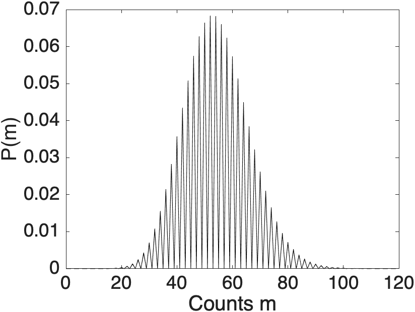
Figure 1: Matrix-P simulations of total photo-count probability (solid lines) versus the exact multi-mode squeezed state photon counting distribution for GBS (dashed lines) for squeezed states with squeezing parameter $\boldsymbol{r}=[0.5,\dots,0.5]$ and a Haar random unitary matrix of size $M=200$. Numerical probabilities are obtained by averaging over ensembles of size $E_{S}=1.2\times 10^{6}$ . Sampling errors and difference errors are both $<6\times 10^{-5}$, and are not visible. A size of $M=10^{6}$ reduced the errors to $\sim 6\times 10^{-6}$, with a maximum probability of 0.0096.

The projection operator for an output photon number pattern $\bm{m}$ in a set $S$ of measurements is

$$\hat{G}\left(\bm{m}\right)=\bigotimes_{i\in S}\frac{1}{m_{i}!}:(\hat{n}{}_{i})^{m_{i}}e^{-\hat{n}{}_{i}}:.$$ (19)

Defining $\hat{n}_{S}=\sum_{i\in S}n_{i}$, and abbreviating $C\equiv\cosh$, $S\equiv\sinh$, the number projector in (19) is rewritten as:

$$\hat{G}\left(\bm{m}\right)=:\left[C\left(\hat{n}_{S}\right)-S\left(\hat{n}_{S}\right)\right]\bigotimes_{i\in S}\frac{\hat{n}^{m_{i}}}{m_{i}!}:.$$ (20)

This allows it to be separated into odd and even powers, giving the result for the parity representation that, if $m=\sum m_{i},$ and $\bar{p}_{m}\equiv\left|1-p_{m}\right|$ , then the c-number function corresponding to $\hat{\bm{G}}\left(\bm{m}\right)$ is:

$$\bm{G}\left(\bm{m}\right)=\left[C\left(n_{S}\right)\bm{T}^{p_{m}}-S\left(n_{S}\right)\bm{T}^{\bar{p}_{m}}\right]\prod_{i\in S}\frac{n_{i}^{m_{i}}}{m_{i}!}.$$ (21)

Applying Eq (15) to the case of the cat-state probability for a single mode with a squeezed state input, only $G_{0}$ is significant because the probability must have even parity. For an odd particle count, one obtains $G_{0}\left(2m+1\right)=0$, as expected, while the c-number pattern projector for even counts is:

$$G_{0}\left(2m\right) =\frac{n^{2m}}{C\left(n\right)\left(2m\right)!}.$$ (22)

The same result holds for the total counts in a multimode case as well. To check this, one can sum over individual projectors to compute the mean particle number, using (22). This agrees with Eq (15), giving the function $\bm{O}\left(n\right)$ that is averaged over the phase-space for a squeezed state, to give the mean photon number $O_{0}\left(n\right)=n\tanh\left(n\right),$ The $\tanh\left(n\right)$ term suppresses results with small $n$ , since parity conservation prohibits an odd count number.

Sampling results of the matrix P-distribution and +P-distribution are given in Fig.(1) and (2) respectively for an exactly soluble 200 mode example, with a known count distribution of [42, 43], where $p=1/(1+\bar{n})$ is the success probability for detecting a photon for $\bar{n}$ mean photons per mode:

$$\mathcal{G}(m)=\begin{cases}\binom{\frac{M}{2}+\frac{m}{2}-1}{\frac{m}{2}}p^{M/2}(1-p)^{m/2},&\text{even}\>m\\ 0.&\text{odd}\>m\end{cases}.$$ (23)

Matrix-P distribution results with $1.2\times 10^{6}$ samples are indistinguishable from exact results with relative errors $\sim 10^{-3}$, in agreement with estimates obtained from the central limit theorem [44]. We have extended this to 10000 modes, larger than any (currently) planned experiments, with similar relative errors. The corresponding P-distribution results have nearly 100% sampling errors when there no losses, due to an extremely skewed distribution of trajectories, requiring much larger sample numbers than is practical.

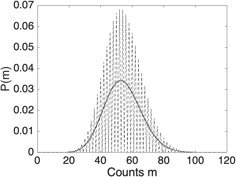
Figure 2: Positive-P phase-space simulations of total photo-count probability (solid lines) versus the exact distribution (dashed lines) for pure state GBS. All other parameters as in Fig(1). Difference errors are $\sim 0.03$, and are clearly visible. This is caused by a skewed distribution leading to sampling errors, requiring enormous sample numbers to reach full convergence, as explained in the SM.

In summary, rapid convergence is obtained for pure-state squeezed vacuum photo-count distributions at large mode number using the matrix-P representation. This will allow precise verification of GBS photon-counting data in low-loss quantum computing experiments. Many more tests than these can be generated. We focus on the pure state, lossless case, because it is the most challenging distribution to treat.

The matrix-P distribution phase-space method may provide the most stringent validation tests to date of such experiments. These improvements in accuracy and scalability are because the method projects only the physical part of Hilbert space. Generating binned approximations as carried out here will make it possible to compare theory with experiment, since the full distributions are too sparse to be measured or calculated.

Further explanations are given in the SM. It is not impossible that the approach described here may prove useful in approximating other #P hard Hafnians. Other symmetries like translational symmetry can be treated as well. This method therefore has wide potential applicability, due to its ability to distinguish global conservation laws from localized quantum entanglement.

Matrix phase-space representations in quantum optics: Supplemental Material

Peter D. Drummond, Alexander S. Dellios, Margaret D. Reid

Convergence properties

In the main text, we showed that the matrix-P representation rapidly converges to the exactly known total photon count probability for multi-mode pure squeezed states with relatively small sampling errors. On the other hand, the positive P-representation did not converge to the exact counts at the same number of samples. In this Supplemental Material, we investigate and explain the different convergence properties of the matrix-P and positive-P representations for applications to GBS.

.1 Exact multi-mode photon statistics: Squeezed states

If each the squeezing parameters of the $j=1,\dots,N$ input squeezed states are equal, $r=r_{1}=\dots=r_{N}$, such that the mean photon number per mode, $n_{j}=\sinh^{2}(r_{j})$, is constant, i.e, $\bar{n}=\bar{n}_{1}=\dots=\bar{n}_{N}$, the multi-mode photon statistics of pure squeezed states can be computed exactly. Here, the set of included modes contains all modes of the linear photonic network. The distribution oscillates for even and odd grouped counts $m$, which arises due to the generation of correlated pairs of squeezed states from a parametric down-conversion process.

In the main text, simulated ensemble means of the matrix-P and positive-P representation were compared to Eq.(23) for a network size of $N=M=200$. To determine whether the positive-P representation can be used to simulate an ideal, lossless GBS with PNR detectors, we simulate a much smaller linear network of size $N=M=50$ with uniform squeezing $\boldsymbol{r}=[0.5,\dots,0.5]$. Comparisons of positive-P moments and the exact distribution are presented in Fig.(3a) for various ensemble sizes. Generally, as is the case with most sampling procedures, in the limit $E_{S}\rightarrow\infty$, positive-P moments converge to moments of an observables distribution. Typically, if the exact tests distribution is a Poissonian or Gaussian distribution, an ensemble size of the order $E_{S}\gtrsim 10^{6}$ is needed for accurate convergence.

When $E_{S}=2.4\times 10^{5}$, no even-odd oscillations are apparent in the positive-P moments, where the distribution is approximately Poissonian with mean equal to that of the exact distributions but with differing variances. This was also the case with simulations presented in the main text. However, there are signs of oscillations beginning to form for small grouped counts of $m\leq 3$. Increasing the ensemble size to $E_{S}=2.4\times 10^{8}$, distinct even-odd oscillations for counts $m\leq 14$ have begun to form, although positive-P moments are still far from their expected probabilities for the majority of these counts.

.2 Sampling error estimates

Sampling error estimates for these simulations were obtained from the central limit theorem Opanchuk et al. [44], by taking sub-ensembles whose means are assumed Gaussian for a sufficiently large number of samples, and then using the variance of the resulting distribution divided by the number of sub-ensembles to estimate the resulting variance in the overall mean. This usually reliable estimate appears to fail in the +P case for these simulations.

This can be seen where sampling errors have noticeably grown for these counts as indicated by the separation between upper and lower lines in Fig.(3a), where each line corresponds to $\pm 1\sigma_{T,j}$ with $\sigma_{T,j}\propto 1/\sqrt{E_{S}}$ being the estimated sampling error. Only for $\mathcal{G}_{S}^{(M)}(m\leq 2)$ does the distribution appear to have converged to within the estimated errors, while probabilities of $\mathcal{G}_{S}^{(M)}(m\geq 14)$ again show no discernible even-odd oscillations. Instead, moments converge to the approximate Poissonian distribution from simulations with $E_{S}=2.4\times 10^{5}$.

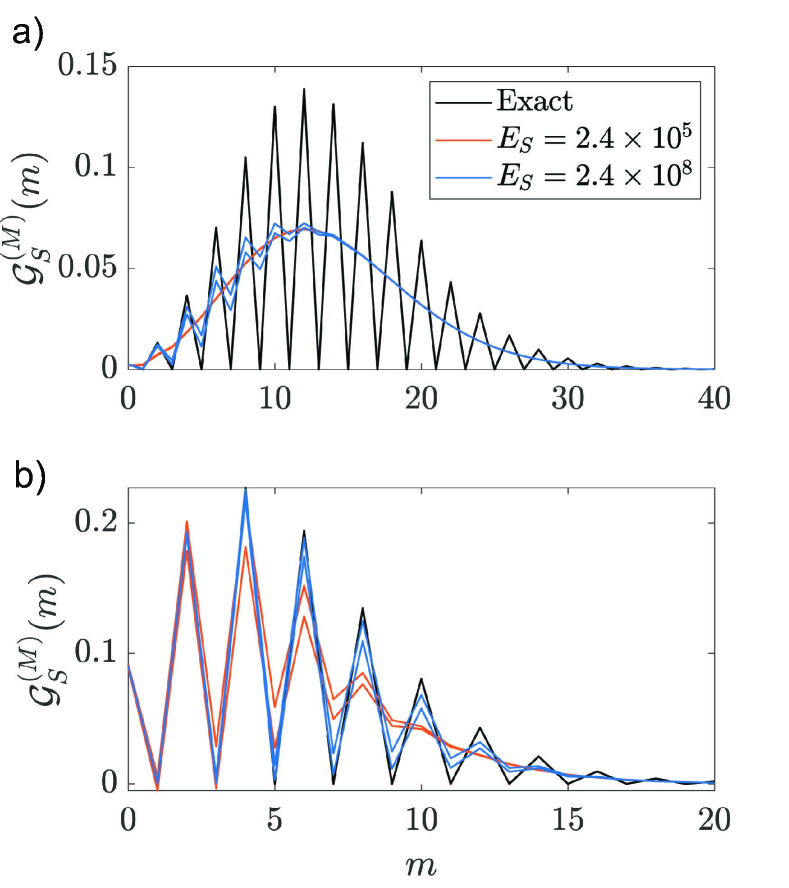
Figure 3: Comparisons of positive-P simulations of the total count distribution versus the exact multi-mode squeezed state photon counting distribution Eq.(23) (solid black line) for two GBS set-ups where pure squeezed states with uniform squeezing parameter $\boldsymbol{r}=[0.5,\dots,0.5]$ are transformed by a Haar random unitary matrix $\boldsymbol{U}$ of size a) $M=N=50$ and b) $M=N=20$. Positive-P moments are obtained by averaging over sample ensembles of size $E_{S}=2.4\times 10^{5}$ (solid orange line) and $E_{S}=2.4\times 10^{8}$ (solid blue line). Upper and lower lines correspond to $\pm 1\sigma_{T,j}$ theoretical sampling errors for the $j$-th photon count bin.

The conservation laws present in such a perfect model causes convergence to be much slower than the rapid convergence obtained with positive P methods for more lossy cases typical of current GTBS experiments. This becomes clearer when we repeat the numerical simulations for a reduced system size of $M=N=20$, where positive-P moments are compared to Eq.(23) in Fig.(3b). In this case, positive-P moments produce the required even-odd count oscillations for most $m$ values. Although better convergence is obtained when $E_{S}=2.4\times 10^{8}$, sampling errors are large in both cases for most $m$ values. Only for $\mathcal{G}_{S}^{(M)}(m\leq 4)$ are sampling errors small enough to not be visible when $E_{S}=2.4\times 10^{8}$.

For reference, Fig.(4) shows comparisons between CMP moments and the exact distribution of the $M=N=20$ mode network simulated in Fig.(3b). Here, an ensemble size of $E_{S}=1.2\times 10^{6}$ is used, where CMP moments converge to the exact distribution with sampling and differences errors of $<10^{-3}$. Although the CMP representation converges with the same sampling and difference errors for smaller ensemble sizes, a larger $E_{S}$ was used for consistency with simulations in the next subsection.

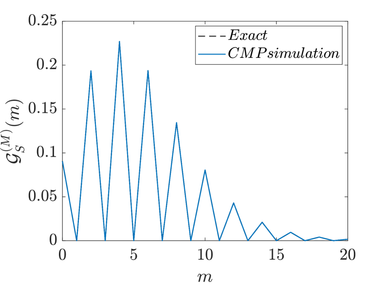
Figure 4: The $M=N=20$ mode lossless network with $\boldsymbol{r}=[0.5,\dots,0.5]$ of Fig.(3b) is simulated using the matrix-P representation for an ensemble size of $E_{S}=1.2\times 10^{6}$ (solid blue line) and compared to the exact photon counting distribution (dashed black line) Eq.(23). Sampling and difference errors are of the order $<10^{-3}$, where the matrix-P moments converge to their exact values for all $m$.

.3 Probability densities of observable stochastic amplitudes

A more detailed picture of the effect the conservations laws have on the convergence properties of the positive-P and matrix-P representations can be obtained by computing the probability density of the stochastic trajectories for a specific observable.

We use a general method of binning the observed phase-space trajectories to estimate the probability density. Coherent amplitudes for some general phase-space observable $O(\boldsymbol{\alpha},\boldsymbol{\beta})$, with corresponding operator $\hat{O}$, are binned into $N_{b}$ equally spaced bins defined on the range $[b_{min},b_{max}]$ with spacing $\Delta_{b}=(b_{max}-b_{min})/N_{b}$ to estimate the probability density as

$$P(O_{j})=\frac{1}{N_{S}\Delta_{b}}\sum_{i=1}^{N_{S}}\bar{O}_{j}^{(i)}.$$ (24)

Here, $\bar{O}_{j}^{(i)}=\frac{1}{N_{R}}\sum_{k=1}^{N_{R}}O_{j}^{(k)}$ is the $i$-th sub-ensemble average over stochastic trajectories of the observable $O_{j}^{(k)}=O(\alpha^{(k)},\beta^{(k)})$ contained in the $j=\left(O^{(k)}-b_{min}\right)/\Delta_{b}$-th bin. There are $N_{S}$ sub-ensembles each of $N_{R}$ individual trajectories, giving $E_{S}=N_{S}N_{R}$, such that $k\leq N_{R}$ and $i\leq N_{S}$ identify individual stochastic trajectories within each sub-ensemble.

The number of samples generated by randomly sampling a phase-space distribution for some initial state is represented by the first number $N_{R}$. The second number $N_{S}$ denotes the number of times this sampling procedure is repeated. In other words, one repeatedly samples from the underlying distribution, producing $N_{R}$ samples for every sub-ensemble, each of which has a sub-ensemble mean.

This division of the ensemble number is common practice in numerical applications of phase-space representations, including the input-output transformation applied in this paper as well as numerical solutions of stochastic differential equations. It is useful as it allows one to estimate sampling errors, and implement multi-core parallel computing. In terms of estimating probability densities, sub-ensembles are utilized for the same purpose, as the final probability density is formed by repeatedly binning the stochastic amplitudes.

In the limit of a large number of trajectories $N_{R}$ per sub-ensemble, the resulting distribution of sub-ensemble means is approximately Gaussian from the central limit theorem. This allows one to use the final variance to estimate the error in the overall mean. An important question, therefore, is just how many samples are needed? This depends on the exact properties of the underlying distribution.

Our simulations in the main text used $E_{S}=1.2\times 10^{6}$, with $N_{S}=120$ sub-ensembles of $N_{R}=10^{4}$ trajectories each, giving maximum errors of $6\times 10^{-5}$ for the matrix-P probabilities. This agrees with the central limit theorem estimates, with errors $\propto 1/\sqrt{E_{S}}.$ The positive-P probabilities had errors up to $\pm 0.03$, $\sim 10^{3}$ times larger, and also much larger than the central limit theorem estimates of standard deviations.

.4 Estimated densities: positive-P trajectories

In order to explain the origin of these differences, we investigate the distribution of the samples themselves. Since the positive-P convergence and sampling errors issues are not present in applications of GBS with threshold detectors we wish to estimate the probability densities of stochastic trajectories for different counts $m$ of the phase-space projector which is relevant to a photon-number resolving experiment:

$$P_{m}=\frac{1}{m!}\left(n\right)^{m}e^{-n}.$$ (25)

In order for the estimated density to be accurate, phase-space moments should be nearly converged to their exact values. Therefore, we start by binning the $E_{S}=2.4\times 10^{8}$ positive-P amplitudes for counts around the mean of the $M=N=20$ mode total count distribution, with odd and even photo-counts of $m=3,4$ (see Fig.(3)). Probability densities $P(P_{m})$ versus the binned $P_{m}$ trajectory values are presented in Fig.(5) for a binning range of $[-100,100]$ with spacing $\Delta_{b}=0.05$, and sub-ensemble sizes $N_{S}=2\times 10^{4}$, $N_{R}=1.2\times 10^{4}$. For simplicity, we have used the notation $P(m)=P(P_{m})$.

In both cases, the probability densities are extremely skewed with long tails. For amplitudes of the $m=4$ count, densities are defined entirely by the $P_{4}\rightarrow\infty$ bins, while amplitudes in the $m=3$ count bin produce an almost mirror-image density. Although the distribution’s tail is defined entirely in the $P_{3}\rightarrow-\infty$ direction, some of the largest probabilities are within the range $P_{3}\in[0,0.5]$ (see insert of Fig.(5)), causing an overlap between the odd and even densities.

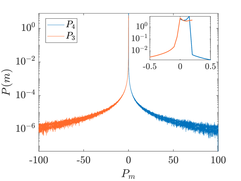
Figure 5: Logarithmic plot of estimated positive-P probability densities $P(m)=P(P_{m})$ versus binned stochastic trajectories of $P_{m}$ for $m=4$ (solid blue line), such that $P_{4}=\frac{1}{4!}\left(n\right)^{4}e^{-n}$, and $m=3$ (solid orange line), with $P_{3}=\frac{1}{3!}\left(n\right)^{3}e^{-n}$. Trajectories are obtained from simulations of the lossless $M=N=20$ mode GBS network with $E_{S}=2.4\times 10^{8}$, whose total count distribution is presented in Fig.(3b). $N_{b}=4\times 10^{3}$ bins are used to obtained density estimates, on a range $[-100,100]$ with spacing $\Delta_{b}=0.05$. Upper and lower lines correspond to $\pm 1\sigma_{T,j}$, which increase as $P_{m}\rightarrow\pm\infty$ due to the exponentially small probabilities one is required to resolve. The inset is a close-up of the bin range $[-0.5,0.5]$, where the probability densities $P(3)$ overlap with the $P(4)$ probabilities. The bins correspond to the largest probability to obtain a specific trajectory value.

The above behavior of oscillating positive and negative skewed densities exists for all even and odd counts, and is due to the $m$ exponent in Eq.(25). When $m=0,2,4,\dots$, negative $n$ intensities are removed causing $P_{m}$ to be strictly positive. Meanwhile for $m=1,3,5,\dots$, negative intensities are conserved allowing $P_{m}$ to be negative for some trajectories. The result is the ensemble mean for odd counts will eventually converge to their expected values of zero.

However, as is clear from Fig.(3), these probabilities are extremely small as $P(P_{3}<0)\rightarrow-\infty$. Hence most trajectories are positive, meaning one must generate an exceedingly large number of samples from the negative skewed tails for the ensemble means to converge. A similar effect arises for trajectories in the even counts. In order for the even count ensemble means to converge to their exact value, they must repeatedly sample from the positive skewed tails as $P(P_{4}>0)\rightarrow\infty$.

In Fig.(3), another interesting result is that ensemble mean convergence is slower for counts in the limit $m\rightarrow\infty$. From Eq.(25), in this limit $m!\rightarrow\infty$, which dominates the exponent $m$, and causes $P_{m}\rightarrow 0$. Therefore, as $m\rightarrow\infty$, one must generate even more samples from the skewed density tails to account for the exponential growth of the factorial.

The combination of these two issues means the number of samples required for convergence will grow exponentially as $M\rightarrow\infty$. Even for a modest system size of $M=N=20$, $E_{S}=2.4\times 10^{8}$ is not enough for full convergence, hence the number of samples required to obtain convergence in the $M=N=200$ simulations in the main text is far too computationally expensive to be practical.

.5 Estimated densities: matrix-P trajectory distributions

Since the positive P-representation is a complete representation with access to the entire Hilbert space, the presence of conservation laws forces one to sample from an exceedingly large sample space of possible photon numbers for highly non-Gaussian distributions such as Eq.(23). As discussed in the main text, projecting onto a smaller Hilbert space allows this computation to become vastly more efficient.

This can be seen in Fig.(6), where we bin the $E_{S}=1.2\times 10^{6}$ matrix-P stochastic amplitudes of $P_{4}$ on the range $[-0.5,0.5]$ with $\Delta_{b}=0.001$ for the total photon count distribution of the $M=N=20$ mode network (see Fig.(4) for distribution). Due to the parity representation expansion, odd counts are always zero, hence probability densities are not necessary in the lossless case.

The significantly smaller binning range is indicative of the limited values of $P_{4}$ for each trajectory. Unlike the positive P-representation, it becomes clearer to see how an ensemble mean of $\mathcal{G}_{S}^{(M)}(m=4)\approx 0.225$ arises from the values of each stochastic trajectory, as the largest probabilities are $P(P_{4}\approx 0.4)$ and $P(P_{4}\approx 0)$. We note an outlier probability of bin $P(P_{4}=-0.001)$ has some non-zero probability, which is due to $P_{4}\ll\Delta_{b}$ that can occur in some cases due to the stochastic nature of phase-space representations.

With conservation laws, sampling from the entire Hilbert space is not necessary. This produces stochastic trajectories that are far from the required ensemble mean, forcing one to generate more phase-space samples to obtain accurate convergence. Once projected onto a smaller, more relevant Hilbert space, the number of samples required reduces significantly as the range of values each trajectory can take is significantly smaller, being limited to only the relevant photon numbers.

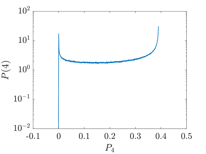
Figure 6: Probability density of binned matrix-P representation outputs for $E_{S}=1.2\times 10^{6}$ trajectories of $P_{4}=\frac{1}{4!}\left(n\right)^{4}e^{-n}$, which corresponds to the mean count value of the $M=N=20$ total count distribution presented in Fig.(4). A binning range of $[-0.5,0.5]$ with $N_{b}=1\times 10^{3}$ equally spaced bins $\Delta_{b}=0.001$ are used to estimate probabilities, although trajectory values are largely only contained within the $[0,0.4]$ bins, with the exception of an outlier bin with $P_{4}\ll 0.001$. The restricted Hilbert space causes the smaller range of values each $P_{4}$ trajectory can take when compared the positive P-representation.

Summary

The difference between the probability densities of the positive-P and matrix-P trajectories are significant. We have discussed the general properties of the densities, and how they affect the sampling requirements of both representations. A variety of probability distributions exist in statistics literature that are highly skewed with long tails. For example, the exponential, log-normal, and power-law distributions are the more commonly used.

For such tail-heavy distributions, both the estimates of the mean and the estimates of errors in the mean using central-limit arguments require an exceptionally large number of samples to give reliable estimates. This is the essential reason for the large sampling errors and the error estimates that are lower than expected.

The improved convergence properties of the matrix-P method are due to the much lower weight tails in its distribution. The physical explanation is that the use of projections allows the conservation laws to be included into the global density matrix $\bm{\Omega}$. This means that a more compact set of phase-space trajectories can be employed, with many orders of magnitude reduction in sampling errors.

References

- Wigner [1932] E. Wigner, Phys. Rev. 40, 749 (1932).
- Husimi [1940] K. Husimi, Proc. Phys. Math. Soc. Jpn. 22, 264 (1940).
- Glauber [1963a] R. J. Glauber, Phys. Rev. 131, 2766 (1963a).
- Sudarshan [1963] E. C. G. Sudarshan, Phys. Rev. Lett. 10, 277 (1963).
- Drummond and Gardiner [1980] P. D. Drummond and C. W. Gardiner, Journal of Physics A: Mathematical and General 13, 2353 (1980).
- Drummond and Chaturvedi [2016] P. D. Drummond and S. Chaturvedi, Physica Scripta 91, 073007 (2016).
- Carter et al. [1987] S. J. Carter, P. D. Drummond, M. D. Reid, and R. M. Shelby, Physical Review Letters 58, 1841 (1987).
- Drummond and Carter [1987] P. D. Drummond and S. J. Carter, J. Opt. Soc. Am. B 4, 1565 (1987).
- Munro and Reid [1993] W. J. Munro and M. D. Reid, Phys. Rev. A 47, 4412 (1993).
- Rosales-Zárate et al. [2014] L. Rosales-Zárate, B. Opanchuk, P. D. Drummond, and M. D. Reid, Physical Review A 90, 022109 (2014).
- Drummond and Corney [1999] P. Drummond and J. Corney, Physical Review A 60, 2661 (1999).
- Kiesewetter et al. [2014] S. Kiesewetter, Q. Y. He, P. D. Drummond, and M. D. Reid, Phys. Rev. A 90, 043805 (2014).
- Takata et al. [2015] K. Takata, A. Marandi, and Y. Yamamoto, Phys. Rev. A 92, 043821 (2015).
- Drummond et al. [2022] P. D. Drummond, B. Opanchuk, A. Dellios, and M. D. Reid, Phys. Rev. A 105, 012427 (2022).
- Kiesewetter and Drummond [2022] S. Kiesewetter and P. D. Drummond, Optics Letters 47, 649 (2022).
- Dellios et al. [2024] A. S. Dellios, M. D. Reid, and P. D. Drummond, arXiv preprint arXiv:2411.11228 (2024).
- Deuar [2005] P. Deuar, First-principles quantum simulations of many-mode open interacting Bose gases using stochastic gauge methods, Ph.D. thesis, The University of Queensland (2005), cond-mat/0507023 .
- Carusotto et al. [2001] I. Carusotto, Y. Castin, and J. Dalibard, Phys. Rev. A 63, 023606 (2001).
- Schrödinger [1935] E. Schrödinger, Naturwissenschaften 23, 823 (1935).
- Deuar and Drummond [2002] P. Deuar and P. D. Drummond, Phys. Rev. A 66, 033812 (2002).
- Gilchrist et al. [1997] A. Gilchrist, C. W. Gardiner, and P. D. Drummond, Phys. Rev. A 55, 3014 (1997).
- Aaronson [2011] S. Aaronson, Proceedings of the Royal Society of London A: Mathematical, Physical and Engineering Sciences 467, 3393 (2011).
- Aaronson and Arkhipov [2013] S. Aaronson and A. Arkhipov, Theory of Computing 9, 143 (2013).
- Hamilton et al. [2017] C. S. Hamilton, R. Kruse, L. Sansoni, S. Barkhofen, C. Silberhorn, and I. Jex, Phys. Rev. Lett. 119, 170501 (2017).
- Deshpande et al. [2022] A. Deshpande, A. Mehta, T. Vincent, N. Quesada, M. Hinsche, M. Ioannou, L. Madsen, J. Lavoie, H. Qi, J. Eisert, D. Hangleiter, B. Fefferman, and I. Dhand, Sci. Adv. 8, eabi7894 (2022).
- Björklund et al. [2019] A. Björklund, B. Gupt, and N. Quesada, Journal of Experimental Algorithmics (JEA) 24, 1 (2019).
- Corney and Drummond [2003] J. F. Corney and P. D. Drummond, Phys. Rev. A 68, 063822 (2003).
- Corney and Drummond [2004] J. F. Corney and P. D. Drummond, Phys. Rev. Lett. 93, 260401 (2004).
- Drummond and Reid [2016] P. D. Drummond and M. D. Reid, Phys. Rev. A 94, 063851 (2016).
- Bargmann [1961] V. Bargmann, Commun. Pure Appl. Math. 14, 187 (1961).
- Glauber [1963b] R. J. Glauber, Phys. Rev. Lett. 10, 84 (1963b).
- Aaronson and Arkhipov [2014] S. Aaronson and A. Arkhipov, Quantum Info. Comput. 14, 1383 (2014).
- Bulmer et al. [2022] J. F. F. Bulmer, B. A. Bell, R. S. Chadwick, A. E. Jones, D. Moise, A. Rigazzi, J. Thorbecke, U.-U. Haus, T. Van Vaerenbergh, R. B. Patel, I. A. Walmsley, and A. Laing, Sci. Adv. 8, eabl9236 (2022).
- Yurke and Stoler [1986] B. Yurke and D. Stoler, Physical review letters 57, 13 (1986).
- Wolinsky and Carmichael [1988] M. Wolinsky and H. J. Carmichael, Phys. Rev. Lett. 60, 1836 (1988).
- Reid and Krippner [1993] M. D. Reid and L. Krippner, Phys. Rev. A 47, 552 (1993).
- Krippner et al. [1994] L. Krippner, W. J. Munro, and M. D. Reid, Phys. Rev. A 50, 4330 (1994).
- Gravina et al. [2023] L. Gravina, F. Minganti, and V. Savona, Prx Quantum 4, 020337 (2023).
- Dellios et al. [2022] A. Dellios, P. D. Drummond, B. Opanchuk, R. Y. Teh, and M. D. Reid, Physics Letters A 429, 127911 (2022).
- Schrödinger [1926] E. Schrödinger, Naturwissenschaften 14, 664 (1926).
- Adam et al. [1994] P. Adam, I. Földesi, and J. Janszky, Physical Review A 49, 1281 (1994).
- Huang and Kumar [1989] J. Huang and P. Kumar, Phys. Rev. A 40, 1670 (1989).
- Zhu and Caves [1990] C. Zhu and C. M. Caves, Phys. Rev. A 42, 6794 (1990).
- Opanchuk et al. [2018] B. Opanchuk, L. Rosales-Zárate, M. D. Reid, and P. D. Drummond, Physical Review A 97, 042304 (2018).