ProtoDepth: Unsupervised Continual Depth Completion with Prototypes

Abstract

We present ProtoDepth, a novel prototype-based approach for continual learning of unsupervised depth completion, the multimodal 3D reconstruction task of predicting dense depth maps from RGB images and sparse point clouds. The unsupervised learning paradigm is well-suited for continual learning, as ground truth is not needed. However, when training on new non-stationary distributions, depth completion models will catastrophically forget previously learned information. We address forgetting by learning prototype sets that adapt the latent features of a frozen pretrained model to new domains. Since the original weights are not modified, ProtoDepth does not forget when test-time domain identity is known. To extend ProtoDepth to the challenging setting where the test-time domain identity is withheld, we propose to learn domain descriptors that enable the model to select the appropriate prototype set for inference. We evaluate ProtoDepth on benchmark dataset sequences, where we reduce forgetting compared to baselines by 52.2% for indoor and 53.2% for outdoor to achieve the state of the art. Project Page: https://protodepth.github.io/.

1 Introduction

Reconstructing three-dimensional (3D) environments facilitates spatial applications such as autonomous navigation, robotic manipulation, and AR/VR. These applications typically utilize platforms equipped with heterogeneous sensors, such as cameras and sparse range sensors (e.g., LiDAR, ToF) which yield RGB images and point clouds. To reconstruct 3D scenes from an ego-centric point of view in the form of depth maps, the point clouds are typically projected onto the image plane. However, their projections tend to be sparse, which is unlike RGB images that comprise irradiance measured at each pixel. These complementary modalities can be used to predict dense depth maps; this multimodal 3D reconstruction task is called depth completion.

Depth completion models can be trained in a supervised (using ground truth) or unsupervised (using Structure-from-Motion) manner. As ground truth is prohibitively expensive to acquire, we subscribe to the unsupervised learning paradigm, which enables one to learn without human intervention. While this suggests the potential to continuously learn, existing models are trained and evaluated on single datasets under the assumption of a stationary data distribution. However, sequences of multiple datasets exhibit non-stationary distributions and are captured by sensors with varying calibrations. Hence, fitting to new data samples inevitably causes the model to “catastrophically forget” [21, 57, 84, 66] previously learned information, where the model performance degrades significantly on data from distributions that it had already observed.

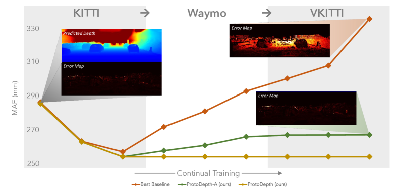
Figure 1: Results on KITTI validation set during continual training on outdoor dataset sequence (KITTI $\rightarrow$ Waymo $\rightarrow$ VKITTI).

To enable pretrained models to adapt to new environments or domains in an unsupervised manner, we consider continual learning, where training strategies aim to mitigate catastrophic forgetting of previously observed training distributions when learning from a continuous stream of non-stationary data. One school of thought is to constrain updates to parameters deemed “important” for previous domains based on a regularization term controlled by a weight chosen as a hyperparameter. Another is to incur memory costs by storing previously observed training data and incorporating them during learning of new domains, akin to rehearsals. The trade-off is in the sensitivity of optimization (and forgetting) to the choice of hyperparameter and in the size of storage and data privacy. Both schools perform updates to the full set of model parameters, which is computationally expensive. Unlike them, we opt to freeze the pretrained model to ensure zero forgetting and learn a small set of parameters, which we term “prototypes,” that modulate the latent features for each new domain encountered.

We model the change in distribution as a domain-specific bias to be learned by global multiplicative and local additive prototypes that transform the latent features to fit the new distribution. In the same vein are learnable prompts or tokens [95] used in continual learning for vision transformers, where the model itself is similarly frozen. Yet, there is no natural scale at which to discretize images, unlike discrete text tokens. In contrast, our proposed prototypes lift the requirements of tokenized inputs and can thus be applied to convolutional neural networks, which are prevalently used in unsupervised depth completion, as well as transformers.

To this end, we propose ProtoDepth, a novel prototype-based method for unsupervised continual depth completion. Instead of prompts in input space, we deploy lightweight prototypes to a frozen pretrained model to encode prototypical information of each domain. These prototypes model global and local biases, where global prototypes learn a transformation from the latent pretrained data distribution to that of the new domain, and local prototypes capture fine-grained features that can be selectively queried depending on the input. Naturally, when the test-time domain identity is known, i.e., domain-incremental, ProtoDepth exhibits no forgetting and learns the new data distribution with high fidelity. We further encode each domain as a descriptor to enable inference when test-time domain identity is withheld, i.e., domain-agnostic, where the prototype set corresponding to the highest affinity domain descriptor for a given sample is chosen.

Our contributions: We propose (1) a novel prototype-based paradigm for unsupervised continual depth completion that incurs no forgetting in the domain-incremental setting, and (2) a prototype set selection mechanism that extends the prototype paradigm to domain-agnostic settings with minimal forgetting. This is facilitated by (3) a novel training objective that learns descriptors for each domain, which can be used to determine the prototype set suitable for inference without knowledge of domain identity. (4) Our method, ProtoDepth, reduces forgetting over baselines by over 50% across six datasets; to the best of our knowledge, this is the first unsupervised continual depth completion method.

2 Related Work

Continual learning is the process of incrementally adapting the weights of a parameterized model to perform new tasks involving non-stationary distributions, while preserving information learned from previous tasks.

Regularization-based methods aim to mitigate forgetting by restricting the plasticity of model parameters that are important for previously learned tasks. [39, 120, 1, 9] introduce regularization terms to the loss function to identify and penalize changes to important weights while new tasks are learned. [70, 16, 42, 121, 17, 31, 45] attempt to preserve output behavior on previous tasks using knowledge distillation [29, 72]. [64, 58, 85, 60] regularize the space of learned functions to encourage similarity between outputs of task-specific heads. However, while they perform well in simpler continual learning settings, regularization-based methods can struggle with more challenging tasks [55] and larger domain shifts between datasets [67, 105].

Rehearsal-based methods use a memory buffer to store a limited amount of data from previous tasks, allowing the model to periodically re-train on this data during continual learning. [9, 71, 28] introduce the strategy of retaining a subset of previous “experiences” (i.e., data) to “replay” (i.e., re-train on) while learning new tasks. [10, 68, 89, 52, 67, 34] employ various sampling strategies, [124, 50, 32] reduce memory by storing latent features rather than inputs, and generative replay methods [76, 59, 3, 107, 69, 73, 62, 36, 26] create synthetic rehearsal data from previous task domains. Some recent works utilize techniques such as self-supervision [8, 63] and knowledge distillation [67, 105, 11, 6]. [12] introduces a rehearsal-based continual single image-based depth estimation method, the first such work for a 3D vision task. Rehearsal-based methods can reduce forgetting but are unsuitable when data storage is limited by memory or privacy constraints [78]. Additionally, their performance degrades significantly as memory buffer size shrinks [8].

Architecture-based methods [56, 75, 91, 35, 74, 116, 44, 51, 65, 123, 37] allocate task-specific parameters or sub-networks, aiming to enable learning of new tasks while minimizing changes to parameters assigned to previous tasks. Most of these methods require task identity to be known at test-time, which prevents their use in the more realistic domain-agnostic setting where new data is not restricted to a certain domain. Other methods [18, 93] rely on a rehearsal buffer in addition to task-specific parameters. Furthermore, architecture-based methods often introduce a significant number of additional parameters for each task [104, 110, 63], which can even exceed the parameter count of the original model [91, 35]. In contrast, our method can perform inference without task identity, does not require a rehearsal buffer, and adds <5% of the original model’s parameters per task.

Prompt-based methods introduce learnable prompts that encode task-specific information. [95] learns a pool of tokens, from which a set is selected using a query mechanism and prepended to the input. [94] refines this by using both task-specific and shared prompts. Subsequent approaches replace prompt selection with an attention mechanism [81] or with intermediate embeddings [38]. However, these prompt-based methods are designed for 2D classification tasks that use vision transformers (ViTs), borrowing the concept of prompting from the field of natural language processing (NLP). The idea of prepending prompts to tokenized inputs does not naturally extend to convolutional neural networks (CNNs), limiting their applicability to 3D vision tasks where CNNs are primarily used. In contrast, our method learns prototypes, which serve as representative features, offering a more intuitive mechanism for adding a lightweight selective bias than prepending abstract prompts in image space. Unlike prompt-based methods, our method is fully architecture-agnostic and can be applied to any model that has a latent space without modifying the underlying architecture.

Prototypes have predominantly been explored in the context of few-shot learning of 2D tasks [82, 48, 112, 47, 24, 25] and representation learning [13, 7, 43]. For continual learning, prototypes have been deployed for supervised classification tasks as discriminative class representations [96, 2, 15, 30, 122, 46]. In contrast, we leverage prototypes as a mechanism for encoding domain-specific information to facilitate continual learning for unsupervised reconstruction.

Unsupervised depth completion is a multimodal, 3D reconstruction problem of predicting a depth map from an image and its associated sparse point cloud. In lieu of training signals from ground-truth depth annotations, unsupervised depth completion methods [54, 77, 101, 102, 100, 111, 115, 33, 49, 41, 99, 19, 80, 20, 97] minimize the reconstruction error of the sparse depth, the reprojection error of the image from temporally adjacent views, and a local smoothness regularizer. Some works [115, 53, 87] utilize synthetic data to learn priors, while other works [100, 101] densify then refine the sparse point cloud by constructing a coarse piecewise scaffolding. [98] uses backprojection layers to map image features to the 3D scene using camera calibration. These methods are prone to catastrophic forgetting in continual learning settings since they must update their learned model weights to fit to new data, causing performance degradation on previously seen data domains. In contrast, our method freezes the entire model and learns a lightweight selective bias for each dataset, allowing it to adapt effectively to new data domains while mitigating forgetting.

UnCLe [23] proposes a benchmark and adapts existing methods [39, 45, 71] for unsupervised continual depth completion. To the best of our knowledge, we propose the first continual learning method for unsupervised depth completion and are the first to explore prototypes in this context.

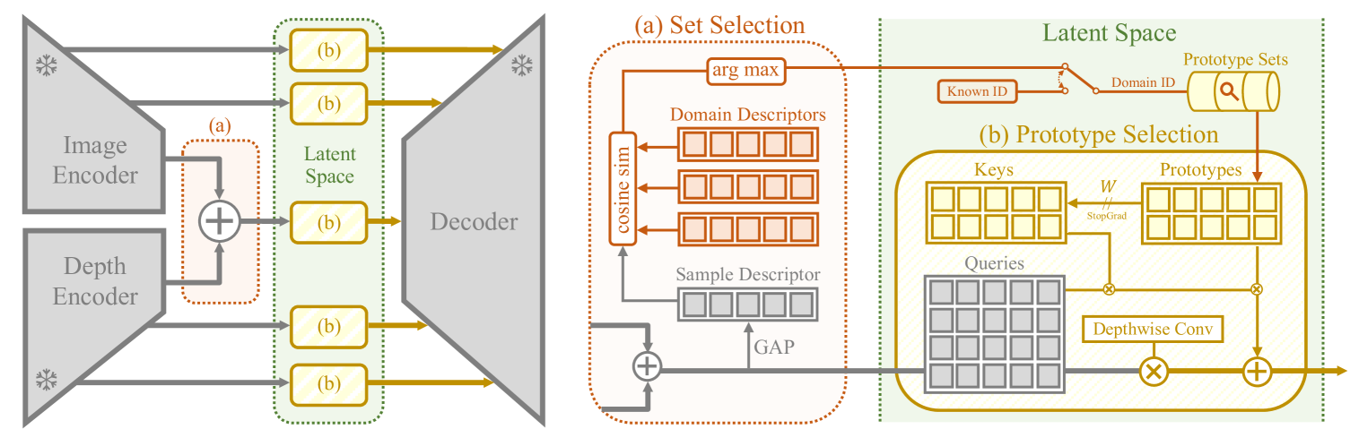
Figure 2: Overview of ProtoDepth. (a) In the agnostic setting, a prototype set is selected by maximizing the cosine similarity between an input sample descriptor and the learned domain descriptors. In the incremental setting, the domain identity is known. (b) At inference, the similarity between the frozen queries and the keys of the selected prototype set determines how the learned prototypes contribute as local (additive) biases to the latent features. Additionally, a global (multiplicative) bias is applied using a $1\times 1$ depthwise convolution.

3 Preliminaries

Unsupervised Depth Completion. Assuming we are given an RGB image $I:\Omega\subset\mathbb{R}^{2}\rightarrow\mathbb{R}^{3}$ and its associated sparse depth map $z:\Omega\rightarrow\mathbb{R}_{+}$ obtained by projecting the sparse point cloud onto the image plane, we wish to train a depth completion model $f_{\theta}$ to predict the dense depth map $\hat{d}$ in an unsupervised manner (i.e., without access to ground-truth depth). Unsupervised depth completion models [54, 100, 101, 98] typically minimize a loss function in the form of Eq.˜1, which comprises a linear combination of three terms:

$$\mathcal{L}=w_{ph}\ell_{ph}+w_{sz}\ell_{sz}+w_{sm}\ell_{sm},$$ (1)

where $\ell_{ph}$ denotes photometric consistency, $\ell_{sz}$ sparse depth consistency, and $\ell_{sm}$ a local smoothness regularizer.

Photometric Consistency term leverages image reconstruction as the training signal. Specifically, given an image $I_{t}$ at time $t$, its reconstruction $\hat{I}_{t\tau}$ from a temporally adjacent image $I_{\tau}$ at time $\tau$ for $\tau\in\{t-1,t+1\}$ is given by

$$\hat{I}_{t\tau}(x,\hat{d},g_{\tau t})=I_{\tau}\big{(}\pi g_{\tau t}K^{-1}\bar{x}\hat{d}(x)\big{)},$$ (2)

where $\bar{x}=[x^{\top},1]^{\top}$ is the homogeneous coordinates of $x\in\Omega$, $K$ is the camera intrinsic calibration matrix, $g_{\tau t}\in SE(3)$ is the estimated relative camera pose matrix from time $t$ to $\tau$, and $\pi$ is the canonical perspective projection matrix. Given $I_{t}$ and its reconstruction $\hat{I}_{t\tau}$, the photometric consistency loss measures the $L1$ difference and structural similarity (SSIM [90]) between $I_{t}$ and $\hat{I}_{t\tau}$:

$$\ell_{ph}=\frac{1}{|\Omega|}\sum_{\tau\in T}\sum_{x\in\Omega} w_{co}|\hat{I}_{t\tau}(x)-I(x)|+$$ (3)

$$w_{st}\big{(}1-\texttt{SSIM}(\hat{I}_{t\tau}(x),I(x))\big{)}.$$

Sparse Depth Consistency. However, photometric reconstruction recovers depth only up to an unknown scale. To ground predictions to a metric scale, we minimize an $L1$ loss between the predicted depth $\hat{d}$ and sparse depth $z$ for $x\in\Omega$ where points exist as denoted by $M:\Omega\mapsto\{0,1\}$:

$$\ell_{sz}=\frac{1}{|\Omega|}\sum_{x\in\Omega}|M(x)\cdot(\hat{d}(x)-z(x))|.$$ (4)

Local Smoothness. To address ambiguities in regions where the predicted depth is not constrained by photometric or sparse depth reconstruction terms, we rely on a regularizer that enforces local smoothness in predictions by applying an $L1$ penalty on the depth gradients in both the $x$-direction ($\partial_{X}$) and $y$-direction ($\partial_{Y}$). To allow for depth discontinuities along object boundaries, these penalties are weighted by their corresponding image gradients, $\lambda_{X}=e^{-|\partial_{X}I_{t}(x)|}$ and $\lambda_{Y}=e^{-|\partial_{Y}I_{t}(x)|}$. Larger image gradients result in smaller weights, allowing for sharp transitions in depth along edges:

$$\ell_{sm}=\frac{1}{|\Omega|}\sum_{x\in\Omega}\lambda_{X}(x)|\partial_{X}\hat{d}(x)|+\lambda_{Y}(x)|\partial_{Y}\hat{d}(x)|.$$ (5)

Unsupervised Continual Depth Completion. For continual learning, we consider a task sequence of domains $\mathcal{D}_{1},\mathcal{D}_{2},\cdots,\mathcal{D}_{T}$. Starting with a depth completion model $f_{\theta}$ pretrained on the initial dataset $\mathcal{D}_{1}$, we aim to incrementally adapt $f_{\theta}$ to each subsequent dataset $\mathcal{D}_{2},\cdots,\mathcal{D}_{k},\cdots,\mathcal{D}_{T}$. The key challenge is to learn the data distribution of each new dataset $\mathcal{D}_{k}$ without “forgetting,” as measured by performance degradation on previously learned datasets $\mathcal{D}_{j<k}$. We denote each dataset as $\mathcal{D}_{k}=\{(I_{k}^{(i)},z_{k}^{(i)},K_{k}^{(i)})\}_{i=1}^{n_{k}}$, which comprises $n_{k}$ training samples of image, sparse depth, and calibration, with no ground-truth depth. We assume that the relative camera pose $g_{t\tau}$ is given, or is estimated; if estimated by a pose network, we allow it to forget as we focus on continual learning for depth completion, and not pose estimation, which is outside the focus of this work.

		Average Forgetting (%)				Average Performance (mm)				SPTO (mm)
Model	Method	MAE	RMSE	iMAE	iRMSE	MAE	RMSE	iMAE	iRMSE	MAE	RMSE	iMAE	iRMSE
VOICED	Finetuned	8.828	6.131	6.951	7.042	63.352	125.28	15.461	35.053	52.453	108.434	15.360	35.357
	EWC [39]	9.439	8.014	5.183	6.174	63.787	126.706	15.229	34.367	53.614	110.956	15.091	34.039
	LwF [45]	8.591	8.456	9.613	21.774	65.135	126.968	16.221	38.002	53.517	108.845	15.402	34.729
	Replay [71]	6.154	4.688	9.471	11.713	64.305	126.714	16.373	36.729	54.326	112.218	16.640	37.671
	ProtoDepth-A	2.439	3.598	4.630	4.519	56.971	118.132	13.554	30.554	47.367	103.015	13.517	31.623
	ProtoDepth	0.000	0.000	0.000	0.000	56.359	115.153	13.589	30.332	46.934	101.326	13.684	31.925
FusionNet	Finetuned	24.928	9.775	32.333	16.799	66.523	130.142	15.829	33.881	54.252	110.666	15.317	33.726
	EWC [39]	11.256	8.782	17.944	17.847	64.487	130.890	15.264	34.203	51.345	109.223	14.276	32.781
	LwF [45]	6.863	2.865	7.336	1.939	61.204	123.573	14.075	30.879	50.159	106.386	13.879	31.608
	Replay [71]	5.702	2.862	12.196	11.186	61.467	125.587	14.750	33.279	50.273	108.608	14.351	33.658
	ProtoDepth-A	1.282	0.686	1.304	0.446	57.742	119.988	13.274	30.139	47.674	104.349	13.128	31.058
	ProtoDepth	0.000	0.000	0.000	0.000	57.486	119.168	13.323	29.936	47.335	102.845	13.091	30.474
KBNet	Finetuned	16.080	15.463	8.188	9.170	58.577	124.606	13.474	31.409	47.890	105.807	13.266	31.742
	EWC [39]	14.915	11.878	10.398	5.640	57.414	122.075	13.741	31.552	48.031	106.661	14.129	33.096
	LwF [45]	9.717	6.324	6.168	5.254	57.511	119.093	14.119	32.165	47.154	103.164	14.304	33.838
	Replay [71]	7.200	4.819	9.202	9.539	56.208	117.848	13.983	32.341	46.700	103.631	13.844	33.326
	ProtoDepth-A	3.204	1.304	4.911	2.943	54.254	115.548	13.201	30.499	45.264	101.097	13.281	31.718
	ProtoDepth	0.000	0.000	0.000	0.000	52.497	113.548	12.845	29.990	44.092	99.788	13.081	31.503

Table 1: Quantitative results on indoor datasets. Models are initially trained on NYUv2 and continually trained on ScanNet, then VOID. Bold indicates the best performance, while underline indicates the second-best performance. Baseline results are obtained from UnCLe [23].

4 Method

We present ProtoDepth, a novel approach for unsupervised continual depth completion that mitigates catastrophic forgetting by leveraging prototype sets as selective biases. Given a pretrained depth completion model $f_{\theta}$, which we freeze to prevent any forgetting, we adapt it to new datasets by deploying lightweight, domain-specific prototype sets that learn to selectively bias the latent features; note that this only adds minimal additional parameters per dataset or domain. Our method is applicable to the domain-incremental (“incremental”) setting, where dataset identity is known at test-time, and the more challenging domain-agnostic (“agnostic”) setting, where the test-time domain identity is unknown, through a proposed prototype set selection mechanism (see Sec.˜4.3).

4.1 Prototype Learning

To enable the model to adapt to new datasets without forgetting, we learn layer-specific prototype sets for each dataset that serve as multiplicative (global) and additive (local) biases in the latent feature space. For simplicity, we consider an input sample from a single dataset $\mathcal{D}_{k}$ at a single layer $l$, which is encoded into the latent features $X\in\mathbb{R}^{h\times w\times c}$. We assume a linear transformation from the learned latent space of $\mathcal{D}_{1}$ to that of $\mathcal{D}_{k}$; hence, we formulate the adaptation as

$$\hat{X}=A\odot X+B,$$ (6)

where $\odot$ denotes a (broadcasted) Hadamard product between the global prototype $A\in\mathbb{R}^{c}$ and the features $X$; $B$ is an additive bias constructed from a set of local prototypes $P$.

To this end, we flatten the latent features $X$ to get $Q\in\mathbb{R}^{(h\times w)\times c}$. Since the model $f_{\theta}$ is frozen, $Q$ serves as a set of $h\times w$ deterministic queries, where each query is a $c$-dimensional vector. We introduce $N$ learnable additive prototypes $P=[p_{1},p_{2},\cdots,p_{N}]^{\top}\in\mathbb{R}^{N\times c}$, where each $p_{i}$ is a $c$-dimensional vector representing a “prototypical” local feature of the dataset. To learn the keys associated with each prototype, we define a projection matrix $W$ that learns to map the prototypes $P$ back into the query space, i.e., the latent feature space. This yields $K\in\mathbb{R}^{N\times c}$, where

$$K=\text{StopGrad}(P)\times W.$$ (7)

StopGrad (stop gradient) facilitates decoupled optimization, enabling prototypes to learn appropriate additive biases while keys learn to assign relevant prototypes to queries. We compute the similarity scores between the queries $Q$ and the keys $K$ using scaled dot-product attention [88]. To obtain the additive bias $b\in\mathbb{R}^{(h\times w)\times c}$, the scores are used to compute a convex combination of prototypes $P$:

$$b=\text{softmax}\left(Q\times K^{\top}\middle/\sqrt{c}\,\right)\times P.$$ (8)

We reshape $b$ back to the spatial dimensions of $X$ to obtain the local additive bias $B\in\mathbb{R}^{h\times w\times c}$. To model the global transformation, we learn a $c$-dimensional multiplicative prototype $A$, applied element-wise as $A\odot X$, which can be efficiently implemented as a $1\times 1$ depthwise convolution. The result is further adapted to the new dataset distribution, still without altering the original model parameters, by incorporating the local domain-specific transformation $B$ as an additive bias, i.e., $\hat{X}=A\odot X+B$. As $f_{\theta}$ is frozen and a new prototype set (local and global prototypes $P_{k}$ and $A_{k}$, and projection matrix $W_{k}$) is learned for each dataset $\mathcal{D}_{k}$, this naturally facilitates continual learning and ensures no forgetting in the incremental setting, where the prototype set corresponding to the domain identity is selected. We further extend this to the agnostic setting in Sec.˜4.3.

4.2 ProtoDepth Architecture

Current unsupervised depth completion models [98, 101, 100] adopt an encoder-decoder CNN architecture, which consists of separate image and sparse depth encoders with skip connections to the decoder. We refer to the bottleneck and the skip connections as the latent space layers (see Fig.˜2).

To extend the prototype mechanism (Sec.˜4.1) across multiple layers, for each new dataset $D_{k}$, we introduce a prototype set of local and global prototypes $P^{(l)}$ and $A^{(l)}$, and projection matrix $W^{(l)}$ for each layer $l$ in the latent space. For each new dataset, the latent feature adaptation (Eqs.˜8 and 6) is applied independently to each layer $l$.

As different modalities in multimodal tasks (e.g., RGB image and sparse depth map in depth completion) may experience varying degrees of covariate shift across domains, we propose to deploy a different number of prototypes $N^{(I)}$ and $N^{(z)}$ for the RGB image and sparse depth modalities, respectively. Based on the observation that RGB images undergo a larger covariate shift than sparse depth [61], we choose $N^{(I)}>N^{(z)}$ to capture their prototypical features; this choice reduces the parameter overhead.

The proposed prototype-based continual learning mechanism operates on the latent feature space and does not depend on the specific architecture of the model. This architecture-agnostic flexibility stems from the fact that our queries $Q\in\mathbb{R}^{(h\times w)\times c}$ mirror the general structure of latent features across commonly used model architectures, where $h\times w$ can be replaced by the number of tokens $n$ in the case of transformers [88]. Thus, it can be applied generically to models with latent feature representations [40, 108], providing a general framework for mitigating catastrophic forgetting across various tasks and modalities.

		Average Forgetting (%)				Average Performance (mm)				SPTO (mm)
Model	Method	MAE	RMSE	iMAE	iRMSE	MAE	RMSE	iMAE	iRMSE	MAE	RMSE	iMAE	iRMSE
VOICED	Finetuned	499.598	162.188	467.472	208.693	1620.429	3072.129	4.040	6.144	914.223	2993.228	1.955	4.503
	EWC [39]	555.925	190.152	540.109	247.943	1796.300	3346.057	4.490	6.685	962.937	3209.759	1.962	4.739
	LwF [45]	631.119	221.535	524.976	233.758	1973.972	3612.700	4.533	6.648	985.995	3236.244	2.062	4.722
	Replay [71]	17.241	4.050	16.662	5.478	524.114	1875.897	1.333	3.359	618.668	2366.577	1.292	3.348
	ProtoDepth-A	2.427	2.863	2.079	2.153	458.520	1832.690	1.133	3.213	548.240	2294.399	1.080	3.159
	ProtoDepth	0.000	0.000	0.000	0.000	445.419	1804.158	1.106	3.169	531.689	2262.943	1.043	3.110
FusionNet	Finetuned	11.336	8.435	17.447	17.991	437.730	1785.212	1.193	3.724	501.362	2138.422	1.111	3.978
	EWC [39]	21.006	10.494	20.431	16.535	431.440	1760.460	1.144	3.181	486.170	2117.030	1.029	2.986
	LwF [45]	12.368	5.202	13.593	13.117	442.878	1759.202	1.178	3.352	526.528	2168.961	1.156	3.451
	Replay [71]	8.290	11.134	2.769	7.975	419.044	1774.361	1.044	3.032	479.168	2122.997	0.966	2.906
	ProtoDepth-A	2.200	2.282	2.602	7.203	404.956	1702.945	1.041	3.028	464.976	2052.413	0.952	2.864
	ProtoDepth	0.000	0.000	0.000	0.000	400.888	1683.202	1.022	2.899	461.043	2048.942	0.932	2.792
KBNet	Finetuned	27.153	18.208	52.969	33.370	469.658	1943.259	1.338	3.683	541.383	2411.169	1.144	3.505
	EWC [39]	23.517	8.583	30.077	18.991	456.828	1806.761	1.221	3.321	526.366	2210.424	1.133	3.158
	LwF [45]	21.184	4.049	43.500	19.951	460.097	1749.734	1.362	3.555	541.932	2142.999	1.359	3.731
	Replay [71]	25.423	29.303	6.362	7.274	454.896	1935.667	1.102	3.203	525.696	2318.363	1.094	3.246
	ProtoDepth-A	4.513	3.100	2.960	1.878	409.903	1730.720	1.045	3.044	478.790	2138.347	1.008	3.066
	ProtoDepth	0.000	0.000	0.000	0.000	401.075	1710.074	1.029	2.993	471.437	2125.957	0.996	3.015

Table 2: Quantitative results on outdoor datasets. Models are initially trained on KITTI and continually trained on Waymo, then VKITTI. Bold indicates the best performance, while underline indicates the second-best performance. Baseline results are obtained from UnCLe [23].

4.3 Prototype Set Selection

As the prototypes are learned for a specific domain, we cannot easily select the appropriate prototype set for inference if the test-time domain identity is withheld, i.e., in the domain-agnostic setting. To address this challenging scenario, we introduce a prototype set selection mechanism that chooses the most relevant prototype set for a given input.

During training, we introduce a domain descriptor $r_{k}\in\mathbb{R}^{c}$ for each dataset $\mathcal{D}_{k}$, which adds negligible overhead in terms of number of parameters. For an input from $\mathcal{D}_{k}$, we obtain a sample descriptor $s_{k}\in\mathbb{R}^{c}$ by applying global average pooling (GAP) to the bottleneck latent features (with channel dimension $c$) before applying the prototype set. Importantly, since both encoders are always frozen during continual training, $s_{k}$ is a deterministic mapping of the input.

For each new dataset $\mathcal{D}_{k}$, we deploy a new domain descriptor $r_{k}$ and freeze all existing learned domain descriptors. The deployed domain descriptor $r_{k}$ is trained by minimizing cosine distance between itself and sample descriptors $s_{k}$ for $\mathcal{D}_{k}$, while maximizing the cosine distance to all other learned domain descriptors $\left\{r_{j\neq k}\right\}$. This naturally yields domain descriptors that are discriminative across datasets, allowing us to use the projection of sample descriptors onto domain descriptors as a prototype set selection mechanism. To this end, we propose to minimize an additional objective:

$$\ell_{dr}=1-(\frac{s_{k}}{||s_{k}||}\cdot\frac{r_{k}}{||r_{k}||})+\frac{1}{w_{jk}}\sum_{j\neq k}(\frac{r_{j}}{||r_{j}||}\cdot\frac{r_{k}}{||r_{k}||}),$$ (9)

where $||\cdot||$ denotes the $L2$-norm and $w_{jk}\propto|j\neq k|$ is a tunable normalization constant. As the previously learned domain descriptors are frozen, their alignment to their respective datasets or domains is preserved, allowing us to continually learn new domain descriptors that can distinguish new datasets. Eq.˜9 is incorporated into Eq.˜1 as an additional term weighted by $w_{dr}$ to yield a novel loss function for training of unsupervised continual depth completion models in the agnostic setting:

$$\mathcal{L}=w_{ph}\ell_{ph}+w_{sz}\ell_{sz}+w_{sm}\ell_{sm}+w_{dr}\ell_{dr}.$$ (10)

At test-time, we compute the sample descriptor $s$ for an input without dataset identity and select the domain descriptor $r_{k^{*}}$ that maximizes cosine similarity with $s$:

$$k^{*}=\arg\max_{k}\,(\frac{s}{||s||}\cdot\frac{r_{k}}{||r_{k}||}).$$ (11)

For each latent space layer, we use the prototype set corresponding to the selected domain descriptor. While this does not eliminate forgetting due to the evolving set of domain descriptors and possible overlap between domains, it does minimize forgetting as each prototype set is learned independently for each dataset, but can still be selectively used for inference without knowing the test-time dataset identity. The trade-off is shown in Tabs.˜1 and 2 (ProtoDepth-A) where we incur forgetting in exchange for the flexibility to support both the incremental and agnostic settings.

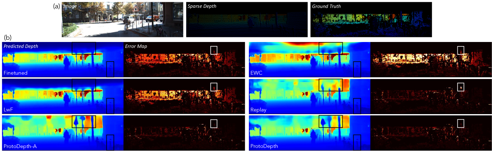
Figure 3: Qualitative comparison of ProtoDepth and baseline methods using VOICED on KITTI after continual training on Waymo. (a) Input sample from KITTI, (b) Baseline methods exhibit significant forgetting, particularly for small-surface-area objects (e.g., street signs and lamp posts) where sparse depth is limited, and photometric priors from KITTI are critical. In contrast, ProtoDepth produces high-fidelity depth predictions, effectively mitigating forgetting despite the large domain gap between KITTI and Waymo.

5 Experiments

Datasets. Indoor dataset sequence: NYUv2 [79] contains household, office, and commercial scenes captured with a Microsoft Kinect; ScanNet [14] is a diverse, large-scale dataset captured using a Structure Sensor; VOID [100] contains laboratory, classroom, and garden scenes captured using XIVO. Outdoor dataset sequence: KITTI [86] is a daytime autonomous driving benchmark captured using a Velodyne LiDAR sensor; Waymo [83] contains road scenes with a wide variety of driving conditions; VKITTI [22] is a synthetic dataset that replicates and augments KITTI scenes.

Models. We evaluate using three recent unsupervised depth completion models in the continual learning setting: VOICED [100], FusionNet [101], and KBNet [98].

Baseline Methods. We compare ProtoDepth against EWC [39], LwF [45], and Experience Replay (“Replay”) [71] as milestone works of their respective class of continual learning approaches. We include full finetuning (“Finetuned”) as a baseline of performance with no continual learning strategy. All baseline methods achieve identical performance in the incremental and agnostic settings.

Evaluation Metrics are computed across four standard depth completion metrics (MAE, RMSE, iMAE, iRMSE). We define the following evaluation metrics in terms of $a_{j}^{k}$, denoting any one of the four depth completion metrics on dataset $\mathcal{D}_{j}$ after training on $\mathcal{D}_{k}$. Given $T$ total datasets:

Average Forgetting ($\bar{F}$) is the scale-invariant mean of how much performance on previous datasets $\mathcal{D}_{j<k}$ deteriorates (i.e., increases in %) after training on each new $\mathcal{D}_{k}$:

$$\bar{F}=\frac{2}{T(T-1)}\,\sum_{k=1}^{T}\,\sum_{j<k}\,\frac{a_{j}^{k}-a_{j}^{j}}{a_{j}^{j}}.$$ (12)

Average Performance ($\bar{\mu}$) is the mean of performance on all seen datasets $\mathcal{D}_{j\leq k}$ after training on each new $\mathcal{D}_{k}$:

$$\bar{\mu}=\frac{2}{T(T+1)}\,\sum_{k=1}^{T}\,\sum_{j\leq k}\,a_{j}^{k}.$$ (13)

Stability-Plasticity Trade-off (SPTO) captures the balance between retaining learned knowledge (stability) and adapting to new domains (plasticity) as a harmonic mean:

$$\text{SPTO}=\frac{2\times S\times P}{S+P},\,\begin{cases}S=\sum_{k=1}^{T}a_{k}^{T}\\[2.5pt] P=\sum_{k=1}^{T}a_{k}^{k}\,,\end{cases}$$ (14)

where $S$ is performance across all datasets after completing training on the dataset sequence, and $P$ is performance on each new dataset after training on it for the first time.

				ScanNet				VOID
Method	$N^{(I)}$	$N^{(z)}$	# Params	MAE	RMSE	iMAE	iRMSE	MAE	RMSE	iMAE	iRMSE
Pretrained	-	-	0M (0%)	4114.04	4626.00	390.78	447.31	42.94	106.39	29.26	64.04
ProtoDepth	1	1	0.24M (3.5%)	19.68$\pm$0.68	60.10$\pm$0.71	10.44$\pm$0.48	27.86$\pm$0.74	37.81$\pm$0.52	93.72$\pm$0.90	22.82$\pm$0.27	52.58$\pm$0.32
	5	5	0.25M (3.6%)	16.49$\pm$0.15	57.51$\pm$0.19	6.84$\pm$0.03	22.07$\pm$0.03	34.02$\pm$0.25	87.72$\pm$0.43	17.92$\pm$0.14	43.95$\pm$0.28
	10	5	0.25M (3.6%)	14.59$\pm$0.17	42.20$\pm$0.09	5.57$\pm$0.14	17.10$\pm$0.15	33.63$\pm$0.23	87.30$\pm$0.57	17.55$\pm$0.32	43.24$\pm$0.63
	10	10	0.25M (3.7%)	15.25$\pm$0.39	43.31$\pm$0.72	5.85$\pm$0.22	17.57$\pm$0.38	34.39$\pm$0.82	88.73$\pm$1.83	18.49$\pm$0.85	45.23$\pm$1.60
	100	100	0.38M (5.5%)	16.35$\pm$0.37	47.61$\pm$0.16	5.90$\pm$0.17	20.11$\pm$0.19	34.29$\pm$0.58	88.22$\pm$0.86	18.16$\pm$0.62	44.51$\pm$1.07

Table 3: Sensitivity study of prototype set sizes ($N^{(I)}$ and $N^{(z)}$) on ProtoDepth using KBNet for indoor datasets (ScanNet and VOID). KBNet is pretrained on the initial dataset (NYUv2). Parameter overhead is reported as a percentage of the full KBNet model’s parameters.

	ScanNet		Waymo
Ablated Component	MAE	RMSE	MAE	RMSE
global prototypes	18.12	58.91	505.01	1715.21
projection matrix $W$	17.59	57.61	495.05	1690.51
decoupled $K$ and $P$	16.36	45.10	491.59	1675.57
no ablations	14.59	42.20	486.95	1664.18

Table 4: Ablation studies using KBNet for indoor and outdoor.

5.1 Main Results

We compare our method, evaluated in both the incremental (ProtoDepth) and agnostic (ProtoDepth-A) settings, against baseline methods for the indoor dataset sequence in Tab.˜1 and for the outdoor dataset sequence in Tab.˜2.

Results in Incremental Setting. In both indoor and outdoor settings, ProtoDepth achieves a 100% improvement in Average Forgetting compared to all baseline methods across all models and metrics. This is, of course, because ProtoDepth exhibits zero forgetting as it freezes all model parameters and learns dataset-specific prototypes. For the indoor sequence, compared to the best baseline method, ProtoDepth improves Average Performance by 5.15% and SPTO by 6.59%, averaged across all models and metrics. Similarly, for the outdoor sequence, we improve Average Performance by 6.88% and SPTO by 6.94%.

To demonstrate the reduced forgetting achieved by ProtoDepth, we qualitatively compare against all baseline methods using VOICED on KITTI after continual training on Waymo (see Fig.˜3). ProtoDepth yields better depth predictions for small-surface-area objects with limited sparse depth measurements for which the model must rely on photometric priors learned from images. Unlike KITTI, which consists exclusively of daytime scenes, Waymo includes many evening and overcast scenes, introducing variations in lighting and pixel intensities. Additionally, Waymo was captured using a higher-resolution camera which causes objects to appear bigger in terms of number of pixels occupied. Due to this large distributional shift, the model forgets the projected shapes of objects in KITTI after training on Waymo, even if the objects exist in both datasets. This forgetting is apparent in the highlighted street sign and lamp posts, where baseline methods struggle to accurately predict depth.

Results in Agnostic Setting. For the indoor sequence, compared to the best baseline method, ProtoDepth-A improves Average Forgetting by 52.22%, Average Performance by 4.26%, and SPTO by 5.40%, averaged across all models and metrics. Notably, ProtoDepth-A outperforms ProtoDepth in some metrics, meaning the model appropriately selects prototypes of different domains when there is domain overlap, thereby enhancing its generalization capabilities.

For the outdoor sequence, ProtoDepth-A shows an average improvement of 53.21% in Average Forgetting across all models and metrics. In contrast to the indoor sequence, ProtoDepth-A does not outperform ProtoDepth in any metric, likely due to the larger domain gaps between the outdoor datasets. Selecting prototypes from a different outdoor dataset is more likely to be erroneous, leading to performance degradation rather than generalization.

Furthermore, we refer back to Fig.˜3 (ProtoDepth-A) for head-to-head comparison of our method against other baselines in the agnostic setting. The error maps for Finetuned, EWC, and LwF display significant errors, indicating substantial forgetting of previously learned information. While Replay yields an improved error map, it still experiences forgetting in small-surface-area objects. For example, Replay fails to reconstruct the upper portions of the highlighted street sign and lamp posts due to forgetting of learned photometric priors from KITTI, whereas ProtoDepth-A recalls them from KITTI prototypes. Additionally, ProtoDepth-A predicts the depth of the highlighted small fence poles with higher fidelity than the incoherent prediction of Replay.

5.2 Design Choice Studies

Prototype Set Sizes. We investigate the impact of varying the prototype set sizes (i.e., number of prototypes) for the image and sparse depth layers (denoted as $N^{(I)}$ and $N^{(z)}$, respectively) on the performance of our method. The set size experiments for the indoor sequence are shown in Tab.˜3, based on which we selected $N^{(I)}=10,N^{(z)}=5$ for the main experiments. Smaller set sizes perform worse as there is insufficient capacity to capture the diversity of features in each dataset. There is also performance degradation with larger set sizes; intuitively, unnecessary additional parameters may learn noise and cause overfitting. Notably, best performance is achieved when $N^{(I)}>N^{(z)}$, which can be attributed to the larger distributional shift between scenes in the image modality compared to the sparse depth modality [61]. Since the bottleneck layer fuses both modalities, we use $N^{(I)}$ for the bottleneck layer prototypes. As a lower bound, we show that the frozen base model pretrained on NYUv2 (“Pretrained”) performs poorly, motivating the need for continual learning. We perform similar set size experiments for the outdoor dataset sequence (see Supp. Mat.), based on which we choose $N^{(I)}=25,N^{(z)}=10$.

Ablations. We assess the impact of the components of ProtoDepth on both indoor (ScanNet) and outdoor (Waymo) in Tab.˜4. Removing the $1\times 1$ depthwise convolutions results in performance degradation, demonstrating their effectiveness as lightweight global prototypes. Learning the keys $K$ independently from the prototypes $P$ without the projection matrix $W$ hurts performance, suggesting that the projection matrix effectively learns to map the prototypes into latent feature space, fulfilling the intended role of keys. Furthermore, performance decreases without the stop gradient operation on $P$ when computing $K$, indicating the importance of decoupled optimization of keys and prototypes.

6 Discussion

ProtoDepth leverages prototypes as a mechanism for mitigating catastrophic forgetting. While we demonstrate it on unsupervised depth completion, ProtoDepth does not assume specific modalities and thus can be relevant to other multimodal problems [109, 113, 118]. Our promising results on both indoor and outdoor domains illustrate the potential for ProtoDepth to enable unsupervised continual learning for multimodal 3D reconstruction. Our architecture-agnostic approach can also be extended to other tasks involving models that produce latent feature representations [40, 119], offering a general framework for continual learning.

Limitations. ProtoDepth relies on knowledge of dataset boundaries to instantiate new prototype sets, which may not be feasible in online training settings where there are no defined boundaries between domains. In the same vein, we do not consider scenarios where domain gaps between datasets are small or where there are significant distributional shifts within a dataset. Addressing these limitations would require mechanisms to dynamically detect domain shifts and instantiate new prototypes when appropriate.

Supplementary Material

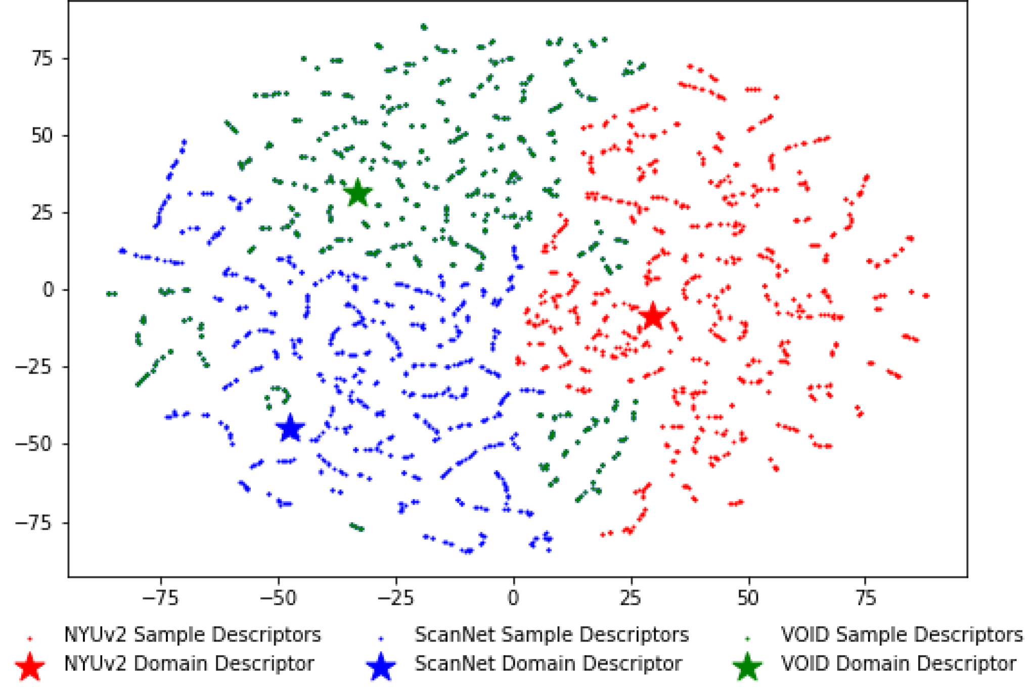
Figure 4: t-SNE plot of KBNet sample descriptors for indoor validation datasets (NYUv2, ScanNet, VOID) and their respective domain descriptors learned during training in the agnostic setting. While most sample descriptors align closely with their respective domain descriptors, some overlap enables cross-domain generalization, improving performance in challenging scenarios.

Appendix A Domain Descriptor Analysis

To better understand the performance of ProtoDepth in the agnostic setting, we analyze the relationship between sample descriptors and learned domain descriptors using the t-SNE visualization shown in Fig.˜4. This analysis is based on the KBNet model trained on the indoor dataset sequence, and it reveals insights into how ProtoDepth selects prototype sets during inference.

Each sample descriptor is computed deterministically using global average pooling (GAP) over the bottleneck features of the frozen model. Since the encoder layers are always frozen during training, the sample descriptors of a certain dataset are a lifelong deterministic function of the features present in that dataset. The domain descriptors, on the other hand, are learned during training to align with the sample descriptors of their respective datasets, enabling effective prototype set selection.

The visualization demonstrates that the majority of sample descriptors for each dataset cluster closely around their respective domain descriptors. This alignment confirms that the training process successfully associates each dataset with its corresponding descriptor at test-time, ensuring accurate prototype selection in the agnostic setting. However, it is noteworthy that some sample descriptors are closer to domain descriptors of other datasets. For example, non-negligible subsets of VOID sample descriptors appear to have higher affinity with the NYUv2 and ScanNet domain descriptors. This overlap introduces a degree of generalization, allowing the model to select prototypes from a different domain if they better align with the input sample’s features.

This ability to adaptively select domain descriptors explains why ProtoDepth achieves superior performance in the agnostic setting than in the incremental setting for certain metrics. By relaxing the constraint of fixed domain identity during inference, the agnostic setting enables the model to exploit cross-domain generalization in cases where overlapping features exist between datasets. While this occurs in only a minority of scenarios, it underscores the utility of allowing the model to flexibly choose prototypes, particularly in instances where the distributional characteristics of one domain may overlap with those of another.

Most importantly, the t-SNE plot clearly illustrates that, despite the presence of some overlap, the domain descriptors remain sufficiently distinct to avoid significant performance degradation due to incorrect prototype selection. Instead, this overlap even facilitates generalization (see Tab.˜8), enabling the model to leverage features from neighboring domains to improve depth completion on difficult samples. This balance between dataset alignment and cross-domain generalization is central to ProtoDepth’s ability to adapt to the challenging domain-agnostic setting.

		Average Forgetting (%)				Average Performance				SPTO
Setting	Method	MAE	RMSE	iMAE	iRMSE	MAE	RMSE	iMAE	iRMSE	MAE	RMSE	iMAE	iRMSE
(1) KBNet	ANCL [37]	9.73	10.75	5.58	16.38	56.89	120.30	13.77	31.85	47.32	103.42	13.88	32.76
	CMP [34]	5.39	5.11	8.25	7.90	55.92	117.83	13.74	31.43	46.03	102.36	13.55	32.03
	Ours	3.20	1.30	4.91	2.94	54.25	115.55	13.20	30.50	45.26	101.10	13.28	31.72
(2) Uformer	Finetuned	87.94	73.61	110.98	852.79	183.24	302.99	51.07	297.92	137.20	238.95	49.54	142.33
	L2P [95]	57.07	43.84	50.82	58.24	171.74	273.75	46.90	121.30	139.08	231.88	51.98	156.41
	Ours	37.15	25.50	31.86	17.04	161.62	255.54	42.38	79.34	133.36	220.68	44.74	84.31
(3) KBNet	ANCL [37]	20.49	8.94	23.11	27.73	438.05	1795.76	1.21	3.56	503.53	2203.44	1.18	3.53
	CMP [34]	15.95	15.47	6.90	7.39	447.09	1887.14	1.09	3.19	507.90	2262.46	1.06	3.21
	Ours	4.51	3.10	2.96	1.88	409.90	1730.72	1.04	3.04	478.79	2138.35	1.01	3.07
(4) KBNet	ANCL [37]	35.10	35.31	18.13	10.04	313.71	1067.35	18.89	30.39	343.06	1129.85	18.66	30.20
	CMP [34]	31.60	36.04	12.63	9.90	307.87	1117.91	16.71	30.41	336.08	1142.94	16.66	30.23
	Ours	20.61	18.75	9.79	6.25	277.04	985.58	15.07	28.42	309.57	1035.55	15.05	28.24
(5)	L2P [95]	69.28	23.25	81.95	48.78	519.72	1458.78	25.65	36.21	470.84	1407.23	25.38	35.45
Uformer	Ours	45.42	7.67	46.18	22.05	451.08	1252.88	22.34	32.00	401.95	1220.67	21.97	31.63

Table 5: Additional quantitative results comparing to recent baselines on indoor, outdoor, and mixed sequences with backbone as denoted:
(1,2) Indoor: NYUv2 $\rightarrow$ ScanNet $\rightarrow$ VOID       (3) Outdoor: KITTI $\rightarrow$ Waymo $\rightarrow$ VKITTI       (4,5) Mixed: KITTI $\rightarrow$ NYUv2 $\rightarrow$ Waymo

Appendix B Transformer Experiments

In the main paper, we stated that ProtoDepth is applicable to any model with a latent space, including both CNNs and transformers. To explore the applicability of ProtoDepth to transformer-based architectures, we adapted Uformer [92], a simple encoder-decoder model consisting entirely of transformer blocks, for depth completion. The model takes as input patchified versions of the image and sparse depth, where inputs from each modality are split into $14\times 14$ patches and embedded as $N\times C$ tokens. We adapted Uformer for depth completion by implementing a dual-encoder structure, with one encoder processing image tokens and the other processing sparse depth tokens. Each encoder contains four transformer blocks. After being processed by the encoders, the tokens from both modalities are concatenated and fed into a shared decoder with four additional transformer blocks. Consistent with the CNN-based models used in the main paper, skip connections are included between each encoder block and its corresponding decoder block, allowing multi-scale features to flow between the encoders and decoder.

For ProtoDepth-A and ProtoDepth, we implemented our method in the exact same way as we do for CNN-based models, applying prototype sets to the latent space layers, i.e., the bottleneck and skip connections. The prototype sets learn global (multiplicative) and local (additive) biases for each layer, adapting the frozen transformer layers to each new dataset while mitigating forgetting. This demonstrates that ProtoDepth is fully architecture-agnostic and can be seamlessly applied to both CNNs and transformers.

A notable inclusion in this section is the prompt-based method L2P [95] (Learning to Prompt), which serves as a representative baseline for prompt-based methods. Prompt-based continual learning methods were not included in the main experiments because all existing unsupervised depth completion models are CNN-based, and prompt-based approaches, which operate by prepending prompts to tokenized inputs, are not applicable to CNNs, which operate directly on images without tokenization, which prevents the straightforward insertion of prompts into the input space. However, with the implementation of Uformer, a transformer-based model, we are now able to evaluate L2P, which is a foundational method for prompt-based continual learning.

For L2P, we implement the method as described in the original paper. Specifically, we use a prompt pool of size $M=20$ and select $N=5$ prompts for each input during training and inference. To adapt L2P for depth completion, we implement their loss term, which pulls selected keys closer to their corresponding queries, and incorporate it into our overall loss function (Eq. (1) in the main paper) with a weight of 0.5, as suggested in [95]. To evaluate in the domain-agnostic setting, where dataset identity is withheld at test time, we train $M=20$ new prompts for each new dataset during continual training. At test-time, the model queries all existing learned prompts.

Appendix C Additional Experiments

In Tab.˜5-(2), we compare to L2P [Wang et al., CVPR ’22] [95], a prompt-based method, where we adapt Uformer for unsupervised depth completion as no transformer-based model currently exists for this task. We have added comparisons to ANCL [Kim et al., CVPR ’23] [37], an architecture-based method, and CMP [Kang et al., CVPR ’24] [34], a rehearsal-based method, on the indoor Tab.˜5-(1) and outdoor Tab.˜5-(3) sequences using the KBNet backbone. ProtoDepth-A (Ours) outperforms all of these recent methods, reaffirming our findings.

In Tab.˜5-(4,5), we add experiments in a mixed setting, where the dataset sequence transitions from outdoor to indoor and back to outdoor. We compare to ANCL, CMP, and L2P in this mixed setting and show that ProtoDepth-A outperforms all of these recent methods.

Tab.˜6 shows that recent depth estimation unified/foundation models, Depth Pro [Bochkovskii et al., 2024] [5] and Depth Anything [Yang et al., CVPR ’24] [114] (fit to metric scale via median scaling) do not outperform ProtoDepth-A (NYU $\rightarrow$ VOID) when evaluated on VOID. This validates the advantage of our method over direct depth estimation. Also of note, Depth Pro and Depth Anything are supervised and semi-supervised, while we are unsupervised.

In continual learning, joint training a larger model (e.g., transformer) on all datasets simultaneously serves as a performance upper bound. Tab.˜7 shows that ProtoDepth-A achieves comparable mean performance to this upper bound on {KITTI, Waymo, VKITTI} using the adapted Uformer. Importantly, we address the scientific question of learning in a sequential manner, where one does not have access to all data at once or must learn a new dataset without breaking backwards-compatibility – a common real-world scenario.

Improved generalization to unseen datasets in the intersection of observed domains helps to motivate our method. Tab.˜8 shows generalization to nuScenes (outdoor) after training on KITTI $\rightarrow$ Waymo $\rightarrow$ VKITTI. ProtoDepth-A outperforms joint training, ANCL, and CMP, demonstrating its ability to leverage domain-specific prototypes to enhance zero-shot generalization.

	MAE	RMSE	iMAE	iRMSE
Depth Anything [114]	49.22	88.74	21.22	51.22
Depth Pro [5]	43.06	93.36	20.80	52.24
Ours	33.66	86.99	17.48	43.02

Table 6: Comparison against depth estimation foundation models.

	MAE	RMSE	iMAE	iRMSE
Ours	686.86	2024.42	1.58	3.52
Upper Bound	671.95	2231.97	1.34	3.52

Table 7: Comparison against joint training (upper bound).

	MAE	RMSE	iMAE	iRMSE
Joint Training	2800.27	6284.63	6.06	11.23
ANCL [37]	2753.07	6195.09	5.69	10.86
CMP [34]	2885.82	6234.33	7.12	13.57
Ours	2697.47	5966.57	5.40	10.58

Table 8: Zero-shot generalization to nuScenes.

Appendix D Dataset Details

Indoor datasets: The NYU Depth V2 [79] (“NYUv2”) dataset comprises 464 diverse indoor scenes from residential, office, and commercial environments captured using a Microsoft Kinect. It contains approximately 400,000 aligned RGB and depth image pairs with a resolution of $640\times 480$. About 1,500 points are sampled for each sparse depth map using the Harris corner detector [27]. This dataset serves as a standard benchmark for indoor depth estimation tasks. For our indoor dataset sequence, we utilize NYUv2 as the initial dataset $\mathcal{D}_{1}$ for pretraining our depth completion models that are subsequently applied to indoor continual learning scenarios. The VOID [100] dataset presents sparse depth maps with $\approx 0.5\%$ density ($\approx$1,500 points), alongside RGB frames from various indoor settings such as laboratories, classrooms, and gardens, totaling approximately 58,000 frames ($640\times 480$) captured via XIVO [20]. VOID is designed to address challenges in areas with minimal texture and significant camera motion, key factors for assessing robustness in indoor depth completion tasks. ScanNet [14], a comprehensive indoor dataset, encompasses over 2.5 million frames paired with RGB-D data. Depth frames in ScanNet are captured at a resolution of $640\times 480$ pixels, whereas the color frames have a higher resolution of $1296\times 968$ pixels. Again, we use the Harris corner detector [27] to subsample $\approx$ 1,500 points for the sparse depth maps. We use a subset of the dataset with approximately 250,000 frames across 706 scenes. For all indoor datasets, we use a training crop size of $416\times 576$. For evaluation, depth values across all of these indoor datasets are constrained between 0.2 and 5 meters.

Outdoor datasets: The KITTI [86] dataset is an established benchmark in autonomous driving that comprises over 93,000 stereo image pairs with a resolution of $1240\times 376$ and sparse LiDAR depth maps ($\approx 5\%$ density), all synchronized and captured across diverse urban and rural landscapes using a Velodyne LiDAR sensor. KITTI is the initial dataset $\mathcal{D}_{1}$ for pretraining our depth completion models for the outdoor dataset sequence. The Waymo Open Dataset [83] (“Waymo”) provides roughly 230,000 high-resolution frames ($1920\times 1280$ and $1920\times 1040$) along with LiDAR point clouds, captured from scenes that encompass a broad spectrum of driving scenarios and conditions. For Waymo, the depth values during evaluation are capped between 0.001 and 80 meters and during training, a crop size of $800\times 640$ is employed. The Virtual KITTI [22] (“VKITTI”) dataset offers synthetic, altered re-creations of KITTI scenes captured from virtual worlds created in Unity, with over 21,000 frames at $1242\times 375$ resolution and dense ground truth depth, facilitating the study of domain adaptation. We apply synthetic weather conditions and view rotations to simulate domain shifts that lead to forgetting. For KITTI and VKITTI, we restrict the depth values during evaluation to between 0.001 and 100 meters and utilize a depth cropping of $240\times 1216$. During training, we use a crop size of $320\times 768$.

Given the differences in image resolutions, crop sizes, and evaluation depths, in addition to the different types of scenes captured and sensors used to collect the datasets, we observe large domain gaps between datasets within each sequence, motivating the need for continual learning. We will release code for reproducibility.

Appendix E Depth Completion Metrics

When we reference depth completion metrics in the main paper, we specifically mean the error metrics outlined below and formulated in Tab.˜9. The metrics include Mean Absolute Error (MAE), Root Mean Squared Error (RMSE), Inverse Mean Absolute Error (iMAE), and Inverse Root Mean Squared Error (iRMSE). MAE measures the average $L1$ difference between predicted and ground-truth depths, providing a straightforward indication of prediction accuracy. RMSE measures $L2$ difference which gives higher weight to larger errors, making it sensitive to outliers and thus a robust measure for practical applications. iMAE and iRMSE, on the other hand, are particularly useful for scenarios where errors in smaller depth values are more critical, as they focus on the relative error in inverse depth. Collectively, these metrics allow for a comprehensive evaluation of a model’s capability to predict depth from input data under varied environmental settings, e.g., indoor and outdoor. We note that lower values indicate better performance for all four error metrics. All results are reported in ‘mm’ (millimeters) unless otherwise specified, providing a clear metric standardization.

Metric	Definition
MAE $\downarrow$	$\frac{1}{|\Omega|}\sum_{x\in\Omega}|\hat{d}(x)-d(x)|$
RMSE $\downarrow$	$\big{(}\frac{1}{|\Omega|}\sum_{x\in\Omega}|\hat{d}(x)-d(x)|^{2}\big{)}^{1/2}$
iMAE $\downarrow$	$\frac{1}{|\Omega|}\sum_{x\in\Omega}|1/\hat{d}(x)-1/d(x)|$
iRMSE $\downarrow$	$\big{(}\frac{1}{|\Omega|}\sum_{x\in\Omega}|1/\hat{d}(x)-1/d(x)|^{2}\big{)}^{1/2}$

Table 9: Error metrics for depth completion. These metrics evaluate the accuracy of predicted depth values $\hat{d}(x)$ compared to ground truth depth values $d(x)$ over the set of pixels $\Omega$.

				Waymo				VKITTI
Method	$N^{(I)}$	$N^{(z)}$	# Params	MAE	RMSE	iMAE	iRMSE	MAE	RMSE	iMAE	iRMSE
Pretrained	-	-	0M (0%)	3930.68	6405.75	9.55	14.34	10527.70	18086.22	17.45	31.50
ProtoDepth	1	1	0.24M (3.5%)	587.92	1900.96	1.41	2.96	937.18	4027.53	1.92	5.82
				$\pm$61.20	$\pm$145.34	$\pm$0.12	$\pm$0.17	$\pm$60.31	$\pm$47.08	$\pm$0.38	$\pm$0.42
	10	10	0.25M (3.7%)	524.76	1667.74	1.28	2.74	686.22	3638.20	0.90	3.50
				$\pm$37.18	$\pm$27.98	$\pm$0.06	$\pm$0.03	$\pm$3.42	$\pm$12.29	$\pm$0.04	$\pm$0.07
	25	10	0.27M (3.9%)	483.92	1656.33	1.19	2.68	676.28	3608.42	0.80	3.25
				$\pm$27.59	$\pm$16.34	$\pm$0.04	$\pm$0.02	$\pm$4.64	$\pm$16.61	$\pm$0.07	$\pm$0.24
	25	25	0.28M (4.0%)	508.60	1688.09	1.23	2.72	680.65	3614.61	0.87	3.51
				$\pm$20.36	$\pm$10.88	$\pm$0.04	$\pm$0.03	$\pm$3.40	$\pm$14.82	$\pm$0.05	$\pm$0.19
	100	100	0.38M (5.5%)	522.39	1711.44	1.27	2.76	686.89	3635.01	0.93	3.53
				$\pm$50.06	$\pm$72.41	$\pm$0.10	$\pm$0.09	$\pm$5.45	$\pm$27.57	$\pm$0.09	$\pm$0.08

Table 10: Sensitivity study of prototype set sizes ($N^{(I)}$ and $N^{(z)}$) on ProtoDepth using KBNet for outdoor datasets (Waymo and VKITTI). KBNet is pretrained on the initial dataset (KITTI). Parameter overhead is reported as a percentage of the full KBNet model’s parameters. Smaller set sizes show suboptimal performance due to insufficient capacity to capture feature diversity, while larger set sizes also degrade performance, likely from overfitting and learning noise.

The results of our experiments are shown in Tab.˜5, which compares ProtoDepth, ProtoDepth-A (agnostic setting), L2P, and full finetuning (“Finetuned”) on the indoor dataset sequence. ProtoDepth achieves superior performance across all metrics, with zero forgetting in the incremental setting, with one exception: ProtoDepth-A outperforms ProtoDepth in one measure, SPTO for iRMSE, highlighting the benefits of its generalization capability. This result is consistent with our earlier observations: by allowing the model to select domain descriptors and prototype sets dynamically at test time, ProtoDepth-A can leverage features from overlapping domains to improve performance on ambiguous samples. This flexibility enables better generalization, which, in certain scenarios, can lead to improved outcomes compared to the fixed domain identity approach used in ProtoDepth.

Notably, ProtoDepth-A outperforms L2P in the agnostic setting, demonstrating the strength of prototype-based adaptation compared to prompt-based approaches. While L2P shows improvements over finetuning, it performs less well than ProtoDepth, which can be attributed to a fundamental limitation of prompt-based methods. These methods rely on learnable prompts or tokens to adapt frozen vision transformer models for continual learning, but there is no natural scale at which to discretize images or choose an appropriate prompt size, unlike the discrete text tokens used in natural language processing. In contrast, ProtoDepth’s prototype-based approach eliminates the need for tokenized inputs, enabling it to operate directly in the latent feature space. This flexibility not only enhances its adaptability across diverse datasets but also allows it to be applied seamlessly to both transformers and convolutional neural networks, which are prevalent in unsupervised depth completion.

Appendix F Outdoor Prototype Set Sizes

We extend our investigation of prototype set sizes (i.e., number of prototypes) for the image and sparse depth layers (denoted as $N^{(I)}$ and $N^{(z)}$, respectively) to the outdoor dataset sequence. The results of these experiments are presented in Tab.˜10. Based on the findings, we select $N^{(I)}=25$ and $N^{(z)}=10$ for the main experiments on the outdoor dataset sequence. Smaller set sizes demonstrate suboptimal performance, as they lack the capacity to adequately capture the diversity of features across datasets. Larger set sizes also result in performance degradation, likely due to the additional parameters learning noise and overfitting to the training data. The best performance is achieved when $N^{(I)}>N^{(z)}$, aligning with our observations in the indoor experiments. This can be attributed to the larger distributional shift between scenes in the image modality compared to the sparse depth modality [61]. For the bottleneck layer, which fuses features from both modalities, we again use $N^{(I)}$ as the prototype set size. As a baseline, we also report the performance of the frozen base model pretrained on KITTI (“Pretrained”), which has no additional parameters or further training. The poor results highlight the necessity of continual learning to adapt to non-stationary data distributions. For both indoor and outdoor settings, the prototype set size analysis is conducted using the KBNet model; we adopt the same prototype set sizes for all other models, as they all have a similar number of parameters.

Appendix G Additional Qualitative Analysis

To illustrate the reduced forgetting achieved by ProtoDepth, we provide a qualitative comparison of depth predictions and error maps for all baseline methods on input samples from NYUv2 after continual training on ScanNet (Fig.˜5 and Fig.˜6). These figures demonstrate how ProtoDepth and ProtoDepth-A consistently outperform the baselines, specifically in reconstructing crowded indoor scenes with sparse depth measurements and challenging lighting conditions.

In Fig.˜5, baseline methods such as Finetuned and EWC exhibit substantial forgetting, resulting in high error concentrations. Finetuned, in particular, struggles to retain photometric priors learned from NYUv2, evident in the poor reconstruction of furniture edges and flat areas with depth gradients. Replay performs marginally better but still fails to recover fine details, as its rehearsal mechanisms are insufficient to address the large distributional shift between NYUv2 and ScanNet. LwF shows improved performance, with fewer errors compared to Finetuned, EWC, and Replay. However, it fails to accurately reconstruct regions with sparse depth measurements (see Sparse Depth), such as the curtain.

ProtoDepth and ProtoDepth-A, on the other hand, produce high-fidelity depth predictions. ProtoDepth benefits from its prototype-based adaptation, effectively preserving features from NYUv2 while adapting to ScanNet. Notably, ProtoDepth-A exhibits comparable performance and even outperforms ProtoDepth in reconstructing certain regions, such as the smooth surface of the curtain. This improvement is due to ProtoDepth-A’s generalization capability, which allows it to dynamically select prototype sets from overlapping domains based on the affinity of domain descriptors, thereby enhancing its ability to handle ambiguous inputs.

Fig.˜6 reinforces these observations with a second example. Once again, baseline methods exhibit significant forgetting, with Finetuned, EWC, and LwF producing poor depth predictions. In contrast, ProtoDepth and ProtoDepth-A produce high-fidelity reconstructions. The well-defined edges between the furniture, floor, and walls in their predictions highlight their ability to preserve learned features while adapting to new domains. ProtoDepth-A, in particular, demonstrates its generalization strength by leveraging overlapping domain features to improve predictions in certain areas, such as the bedpost edges.

Overall, these qualitative results underscore the ability of ProtoDepth to mitigate catastrophic forgetting and produce high-fidelity depth predictions. By effectively combining domain-specific adaptation and cross-domain generalization, ProtoDepth-A outperforms baseline methods, even under significant domain shifts between NYUv2 and ScanNet.

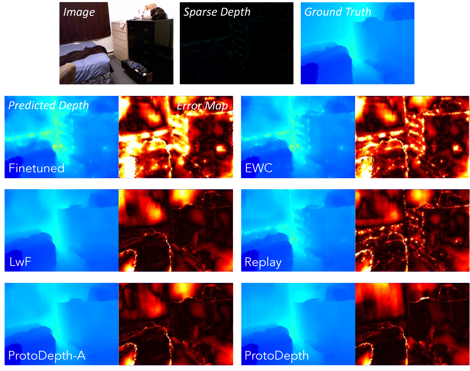
Figure 5: Qualitative comparison (1 of 2) of ProtoDepth and baseline methods using FusionNet on NYUv2 after continual training on ScanNet. Top row: Input sample from NYUv2. Following rows: Output depth and error maps (relative to ground-truth) of same sample from NYUv2 after continual training on ScanNet using each continual learning method.

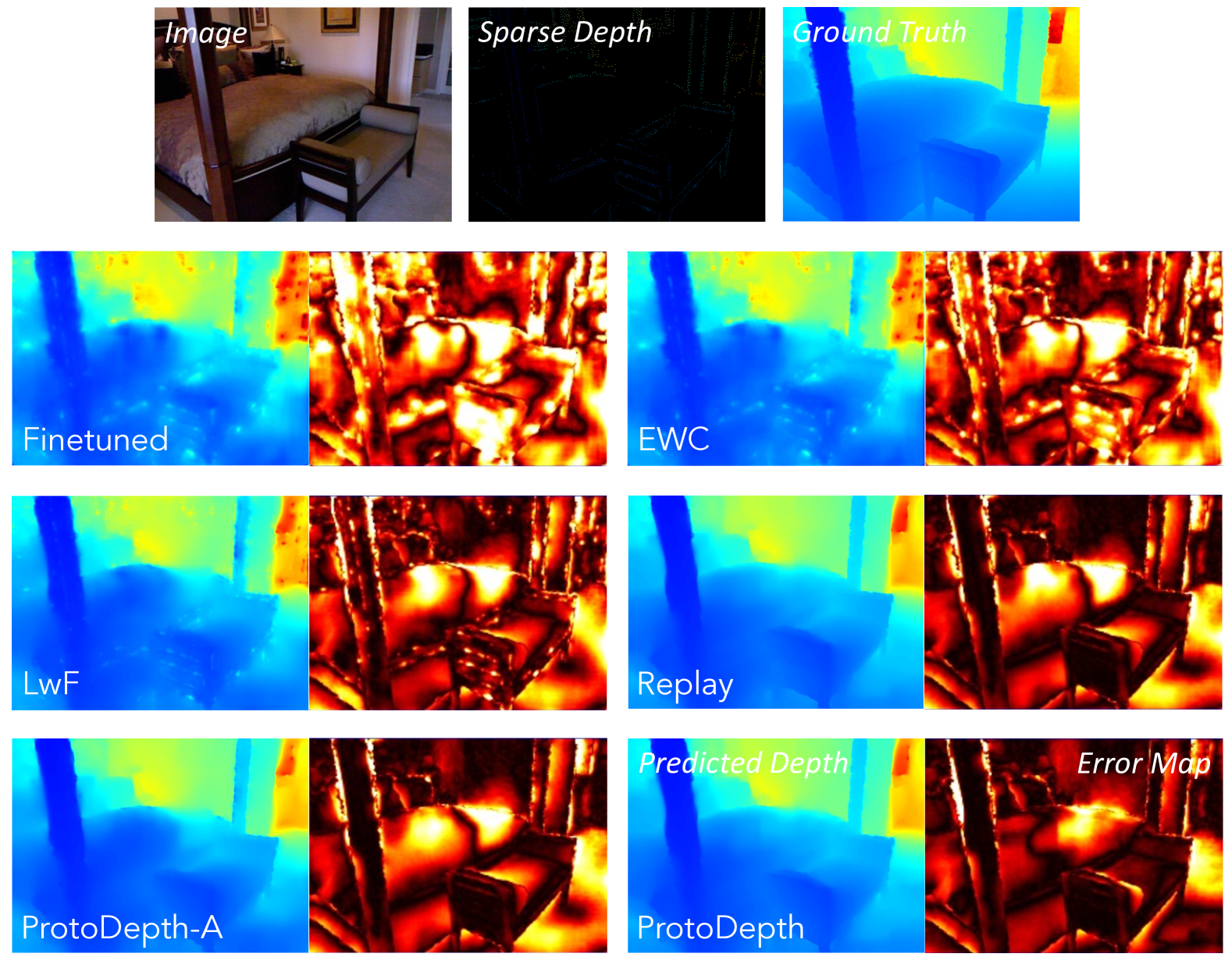
Figure 6: Qualitative comparison (2 of 2) of ProtoDepth and baseline methods using FusionNet on NYUv2 after continual training on ScanNet. Top row: Input sample from NYUv2. Following rows: Output depth and error maps (relative to ground-truth) of same sample from NYUv2 after continual training on ScanNet using each continual learning method.

Appendix H Training Time Comparison

Tab.˜11 presents the training time per epoch for each continual learning method on both indoor (ScanNet and VOID) and outdoor (Waymo and VKITTI) datasets using KBNet. These experiments were conducted with a fixed batch size of 12 for indoor datasets and 8 for outdoor datasets, on a single NVIDIA GeForce RTX 3090 GPU. This standardized setup ensures a fair comparison across all methods. The training times vary across datasets because they are measured per epoch, and each training set contains a different number of frames, as detailed in Appendix˜D.

	Training Time per Epoch (mins)
Method	ScanNet	VOID	Waymo	VKITTI
Finetuned	165.8	35.4	84.7	17.3
EWC	168.2	35.9	85.0	18.5
LwF	170.7	38.1	85.4	20.3
Replay	182.9	40.4	88.8	23.0
ProtoDepth-A	92.5	17.9	40.3	10.7
ProtoDepth	85.3	15.7	37.9	9.6

Table 11: Training times (minutes per epoch) with KBNet for each continual learning method on both indoor and outdoor datasets.

ProtoDepth and ProtoDepth-A demonstrate significant improvements in computational efficiency, with training times roughly half those of the baseline methods. This efficiency can be attributed to ProtoDepth’s approach of freezing the backbone model and training only the prototype sets, which are applied to the latent space layers (i.e., bottleneck and skip connections). Thus, backpropagation computations are restricted to parameters from the output layer back only to the latent space layers. Since the parameters involved are approximately half of the total parameters, ProtoDepth requires fewer gradient computations compared to methods like EWC, LwF, and Replay that calculate gradients and update parameters across the entire model.

ProtoDepth achieves slightly faster training times than ProtoDepth-A. This difference arises because ProtoDepth-A requires additional computations to train the domain descriptors, which involves calculating and optimizing cosine similarity between sample descriptors and domain descriptors during training. ProtoDepth avoids this step, resulting in a small yet consistent reduction in training time.

Among the baseline methods, Finetuned is the fastest, training slightly faster than EWC, LwF, and Replay. This is because finetuning does not involve the additional regularization or distillation used by EWC and LwF, nor does it use a memory buffer like Replay. However, the simplicity of full finetuning comes at the cost of increased catastrophic forgetting, as evidenced by its consistently poor performance in the main experiments.

The reduced training times of ProtoDepth and ProtoDepth-A are particularly important for real-world applications, where computational efficiency is crucial. By restricting updates to the latent space, ProtoDepth not only reduces computational overhead but also does so while achieving state-of-the-art performance. This efficiency is critical for resource-constrained environments, or scenarios requiring fast adaptation to new datasets. These results highlight ProtoDepth’s ability to deliver both high performance and practical advantages in training time, underscoring its suitability for continual learning tasks.

Appendix I More Ablation Studies

To further evaluate the importance of prototype sets in ProtoDepth, we conduct additional ablation studies to assess the impact of removing prototype sets from different modalities and latent space layers. Specifically, we analyze the role of prototype sets applied to the image features, sparse depth features, and the bottleneck features. The results, shown in Tab.˜12, are evaluated on ScanNet (indoor dataset) and Waymo (outdoor dataset) using KBNet.

The results highlight that removing prototype sets from any of these components significantly degrades performance. When image prototype sets are ablated, we observe a sharp increase in both MAE and RMSE, particularly for ScanNet, where MAE rises from 14.59 to 35.06. This degradation demonstrates the importance of capturing domain-specific biases in image features, as images undergo larger distributional shifts between domains compared to sparse depth, such as changes in lighting, textures, and color distributions.

Similarly, removing the sparse depth prototype sets also results in noticeable performance drops, with MAE increasing from 14.59 to 32.07 for ScanNet. While sparse depth features may exhibit smaller distributional shifts compared to image features, these features are crucial for anchoring the model to the metric scale of the depth predictions. Without the sparse depth prototypes, the model struggles to adapt effectively to the unique distribution of sparse point clouds in each new dataset.

The bottleneck prototype sets play a critical role as well, as they adapt the fused representations of both image and sparse depth modalities. Ablating the bottleneck prototypes leads to performance degradation, although the impact is less severe than removing the image or sparse depth prototypes. For instance, MAE increases from 14.59 to 19.03 for ScanNet when bottleneck prototypes are removed. This suggests that while the bottleneck prototypes contribute to the overall performance, much of the adaptation occurs in the modality-specific layers.

Notably, when all prototype sets are included (no ablations), ProtoDepth achieves the best performance across both datasets, with significantly lower error metrics compared to any ablated configuration. These results validate the design choice of applying prototype sets to both modality-specific features (image and sparse depth) and their fused representations (bottleneck).

	ScanNet		Waymo
Ablated Component	MAE	RMSE	MAE	RMSE
image prototype sets	35.06	88.23	542.16	1703.01
sparse depth prototype sets	32.07	84.39	537.37	1762.31
bottleneck prototype sets	19.03	60.32	502.21	1680.87
no ablations	14.59	42.20	486.95	1664.18

Table 12: Ablation studies on prototype sets for different modalities using KBNet for indoor (ScanNet) and outdoor (Waymo).

Appendix J Discussion

Accurate 3D reconstruction [40, 87, 109] is crucially important for applications that rely on precise perception of surrounding environments [119, 108]. One key challenge in this domain is monocular depth estimation (MDE) [5, 41, 97, 99, 106, 114], which aims to recover metric depth from a single image. However, MDE is fundamentally challenging due to scale ambiguity, making it an inherently ill-posed problem. To overcome this challenge, synchronized complementary modalities—such as LiDAR [19, 100, 98], radar [80], inertial sensors [20], additional cameras [103, 4], and even language [118, 117]—can provide additional cues to resolve scale ambiguity. In particular, LiDAR offers high-precision depth measurements that are relatively dense compared to other time-of-flight sensors such as radar, making it a valuable modality for resolving scale ambiguity and enhancing metric depth estimation accuracy. This task of LiDAR-Camera depth estimation, specifically, is commonly referred to as depth completion [102, 101, 115, 49]. In our work, ProtoDepth, we introduce an unsupervised continual depth completion [23] framework that leverages prototypes to continuously learn in challenging and dynamic environments. Unlike traditional approaches that rely on fully supervised training on stationary datasets, ProtoDepth adapts continuously across domains, demonstrating improved generalization without the need for expensive, inaccurate ground truth. Our comprehensive results demonstrate that ProtoDepth effectively mitigates catastrophic forgetting for depth completion, making it a promising solution for real-world applications in autonomous driving, augmented/virtual reality, robotics, and general scene understanding.

References

- Aljundi et al. [2018] Rahaf Aljundi, Francesca Babiloni, Mohamed Elhoseiny, Marcus Rohrbach, and Tinne Tuytelaars. Memory aware synapses: Learning what (not) to forget. In Proceedings of the European conference on computer vision (ECCV), pages 139–154, 2018.
- Asadi et al. [2023] Nader Asadi, MohammadReza Davari, Sudhir Mudur, Rahaf Aljundi, and Eugene Belilovsky. Prototype-sample relation distillation: towards replay-free continual learning. In International Conference on Machine Learning, pages 1093–1106. PMLR, 2023.
- Ayub and Wagner [2021] Ali Ayub and Alan R Wagner. Eec: Learning to encode and regenerate images for continual learning. In 9th International Conference on Learning Representations, ICLR 2021, 2021.
- Berger et al. [2022] Zachary Berger, Parth Agrawal, Tian Yu Liu, Stefano Soatto, and Alex Wong. Stereoscopic universal perturbations across different architectures and datasets. In Proceedings of the IEEE/CVF Conference on Computer Vision and Pattern Recognition, pages 15180–15190, 2022.
- Bochkovskii et al. [2024] Aleksei Bochkovskii, AmaÃĢl Delaunoy, Hugo Germain, Marcel Santos, Yichao Zhou, Stephan R Richter, and Vladlen Koltun. Depth pro: Sharp monocular metric depth in less than a second. arXiv preprint arXiv:2410.02073, 2024.
- Buzzega et al. [2020] Pietro Buzzega, Matteo Boschini, Angelo Porrello, Davide Abati, and Simone Calderara. Dark experience for general continual learning: a strong, simple baseline. Advances in neural information processing systems, 33:15920–15930, 2020.
- Caron et al. [2020] Mathilde Caron, Ishan Misra, Julien Mairal, Priya Goyal, Piotr Bojanowski, and Armand Joulin. Unsupervised learning of visual features by contrasting cluster assignments. Advances in neural information processing systems, 33:9912–9924, 2020.
- Cha et al. [2021] Hyuntak Cha, Jaeho Lee, and Jinwoo Shin. Co2l: Contrastive continual learning. In Proceedings of the IEEE/CVF International conference on computer vision, pages 9516–9525, 2021.
- Chaudhry et al. [2018] Arslan Chaudhry, Puneet K Dokania, Thalaiyasingam Ajanthan, and Philip HS Torr. Riemannian walk for incremental learning: Understanding forgetting and intransigence. In Proceedings of the European conference on computer vision (ECCV), pages 532–547, 2018.
- Chaudhry et al. [2019] Arslan Chaudhry, Marcus Rohrbach, Mohamed Elhoseiny, Thalaiyasingam Ajanthan, Puneet K Dokania, Philip HS Torr, and Marc’Aurelio Ranzato. On tiny episodic memories in continual learning. arXiv preprint arXiv:1902.10486, 2019.
- Chaudhry et al. [2021] Arslan Chaudhry, Albert Gordo, Puneet Dokania, Philip Torr, and David Lopez-Paz. Using hindsight to anchor past knowledge in continual learning. In Proceedings of the AAAI conference on artificial intelligence, pages 6993–7001, 2021.
- Chawla et al. [2024] Hemang Chawla, Arnav Varma, Elahe Arani, and Bahram Zonooz. Continual learning of unsupervised monocular depth from videos. In Proceedings of the IEEE/CVF Winter Conference on Applications of Computer Vision, pages 8419–8429, 2024.
- Chen et al. [2019] Chaofan Chen, Oscar Li, Daniel Tao, Alina Barnett, Cynthia Rudin, and Jonathan K Su. This looks like that: deep learning for interpretable image recognition. Advances in neural information processing systems, 32, 2019.
- Dai et al. [2017] Angela Dai, Angel X Chang, Manolis Savva, Maciej Halber, Thomas Funkhouser, and Matthias Nießner. Scannet: Richly-annotated 3d reconstructions of indoor scenes. In Proceedings of the IEEE conference on computer vision and pattern recognition, pages 5828–5839, 2017.
- De Lange and Tuytelaars [2021] Matthias De Lange and Tinne Tuytelaars. Continual prototype evolution: Learning online from non-stationary data streams. In Proceedings of the IEEE/CVF international conference on computer vision, pages 8250–8259, 2021.
- Dhar et al. [2019] Prithviraj Dhar, Rajat Vikram Singh, Kuan-Chuan Peng, Ziyan Wu, and Rama Chellappa. Learning without memorizing. In Proceedings of the IEEE/CVF conference on computer vision and pattern recognition, pages 5138–5146, 2019.
- Douillard et al. [2020] Arthur Douillard, Matthieu Cord, Charles Ollion, Thomas Robert, and Eduardo Valle. Podnet: Pooled outputs distillation for small-tasks incremental learning. In Proceedings of the IEEE/CVF Conference on Computer Vision and Pattern Recognition (CVPR), pages 1951–1960, 2020.
- Douillard et al. [2022] Arthur Douillard, Alexandre Ramé, Guillaume Couairon, and Matthieu Cord. Dytox: Transformers for continual learning with dynamic token expansion. In Proceedings of the IEEE/CVF Conference on Computer Vision and Pattern Recognition, pages 9285–9295, 2022.
- Ezhov et al. [2024] Vadim Ezhov, Hyoungseob Park, Zhaoyang Zhang, Rishi Upadhyay, Howard Zhang, Chethan Chinder Chandrappa, Achuta Kadambi, Yunhao Ba, Julie Dorsey, and Alex Wong. All-day depth completion. In 2024 IEEE/RSJ International Conference on Intelligent Robots and Systems (IROS). IEEE, 2024.
- Fei et al. [2019] Xiaohan Fei, Alex Wong, and Stefano Soatto. Geo-supervised visual depth prediction. IEEE Robotics and Automation Letters, 4(2):1661–1668, 2019.
- French [1999] Robert M French. Catastrophic forgetting in connectionist networks. Trends in cognitive sciences, 3(4):128–135, 1999.
- Gaidon et al. [2016] Adrien Gaidon, Qiao Wang, Yohann Cabon, and Eleonora Vig. Virtual worlds as proxy for multi-object tracking analysis. In Proceedings of the IEEE conference on computer vision and pattern recognition, pages 4340–4349, 2016.
- Gangopadhyay et al. [2024] Suchisrit Gangopadhyay, Xien Chen, Michael Chu, Patrick Rim, Hyoungseob Park, and Alex Wong. Uncle: Unsupervised continual learning of depth completion. arXiv preprint arXiv:2410.18074, 2024.
- Garcia and Bruna [2018] Victor Garcia and Joan Bruna. Few-shot learning with graph neural networks. In 6th International Conference on Learning Representations, ICLR 2018, 2018.
- Gidaris and Komodakis [2018] Spyros Gidaris and Nikos Komodakis. Dynamic few-shot visual learning without forgetting. In Proceedings of the IEEE conference on computer vision and pattern recognition, pages 4367–4375, 2018.
- Gopalakrishnan et al. [2022] Saisubramaniam Gopalakrishnan, Pranshu Ranjan Singh, Haytham Fayek, Savitha Ramasamy, and Arulmurugan Ambikapathi. Knowledge capture and replay for continual learning. In Proceedings of the IEEE/CVF winter conference on applications of computer vision, pages 10–18, 2022.
- Harris and Stephens [1988] Christopher G. Harris and M. J. Stephens. A combined corner and edge detector. In Alvey Vision Conference, 1988.
- Hayes et al. [2019] Tyler L Hayes, Nathan D Cahill, and Christopher Kanan. Memory efficient experience replay for streaming learning. In 2019 International Conference on Robotics and Automation (ICRA), pages 9769–9776. IEEE, 2019.
- Hinton [2015] Geoffrey Hinton. Distilling the knowledge in a neural network. arXiv preprint arXiv:1503.02531, 2015.
- Ho et al. [2023] Stella Ho, Ming Liu, Lan Du, Longxiang Gao, and Yong Xiang. Prototype-guided memory replay for continual learning. IEEE Transactions on Neural Networks and Learning Systems, 2023.
- Hou et al. [2019] Saihui Hou, Xinyu Pan, Chen Change Loy, Zilei Wang, and Dahua Lin. Learning a unified classifier incrementally via rebalancing. In Proceedings of the IEEE/CVF Conference on Computer Vision and Pattern Recognition (CVPR), pages 831–839, 2019.
- Iscen et al. [2020] Ahmet Iscen, Jeffrey Zhang, Svetlana Lazebnik, and Cordelia Schmid. Memory-efficient incremental learning through feature adaptation. In Computer Vision–ECCV 2020: 16th European Conference, Glasgow, UK, August 23–28, 2020, Proceedings, Part XVI 16, pages 699–715. Springer, 2020.
- Jeon et al. [2022] Jinwoo Jeon, Hyunjun Lim, Dong-Uk Seo, and Hyun Myung. Struct-mdc: Mesh-refined unsupervised depth completion leveraging structural regularities from visual slam. IEEE Robotics and Automation Letters, 7(3):6391–6398, 2022.
- Kang et al. [2024] DaeJun Kang, Dongsuk Kum, and Sanmin Kim. Continual learning for motion prediction model via meta-representation learning and optimal memory buffer retention strategy. In Proceedings of the IEEE/CVF Conference on Computer Vision and Pattern Recognition, pages 15438–15448, 2024.
- Ke et al. [2020] Zixuan Ke, Bing Liu, and Xingchang Huang. Continual learning of a mixed sequence of similar and dissimilar tasks. Advances in neural information processing systems, 33:18493–18504, 2020.
- Kemker and Kanan [2018] Ronald Kemker and Christopher Kanan. Fearnet: Brain-inspired model for incremental learning. In International Conference on Learning Representations, 2018.
- Kim et al. [2023] Sanghwan Kim, Lorenzo Noci, Antonio Orvieto, and Thomas Hofmann. Achieving a better stability-plasticity trade-off via auxiliary networks in continual learning. In Proceedings of the IEEE/CVF Conference on Computer Vision and Pattern Recognition, pages 11930–11939, 2023.
- Kim et al. [2024] Youngeun Kim, Yuhang Li, and Priyadarshini Panda. One-stage prompt-based continual learning. In European Conference on Computer Vision, pages 163–179. Springer, 2024.
- Kirkpatrick et al. [2017] James Kirkpatrick, Razvan Pascanu, Neil Rabinowitz, Joel Veness, Guillaume Desjardins, Andrei A Rusu, Kieran Milan, John Quan, Tiago Ramalho, Agnieszka Grabska-Barwinska, et al. Overcoming catastrophic forgetting in neural networks. Proceedings of the national academy of sciences, 114(13):3521–3526, 2017.
- Lao et al. [2024a] Dong Lao, Yangchao Wu, Tian Yu Liu, Alex Wong, and Stefano Soatto. Sub-token vit embedding via stochastic resonance transformers. In International Conference on Machine Learning. PMLR, 2024a.
- Lao et al. [2024b] Dong Lao, Fengyu Yang, Daniel Wang, Hyoungseob Park, Samuel Lu, Alex Wong, and Stefano Soatto. On the viability of monocular depth pre-training for semantic segmentation. In European Conference on Computer Vision. Springer, 2024b.
- Lee et al. [2019] Kibok Lee, Kimin Lee, Jinwoo Shin, and Honglak Lee. Overcoming catastrophic forgetting with unlabeled data in the wild. In Proceedings of the IEEE/CVF International Conference on Computer Vision, pages 312–321, 2019.
- Li et al. [2021] Junnan Li, Pan Zhou, Caiming Xiong, and Steven Hoi. Prototypical contrastive learning of unsupervised representations. In International Conference on Learning Representations, 2021.
- Li et al. [2019] Xilai Li, Yingbo Zhou, Tianfu Wu, Richard Socher, and Caiming Xiong. Learn to grow: A continual structure learning framework for overcoming catastrophic forgetting. In International conference on machine learning, pages 3925–3934. PMLR, 2019.
- Li and Hoiem [2017] Zhizhong Li and Derek Hoiem. Learning without forgetting. In Proceedings of the IEEE conference on computer vision and pattern recognition, pages 5077–5086, 2017.
- Li et al. [2024] Zhuowei Li, Long Zhao, Zizhao Zhang, Han Zhang, Di Liu, Ting Liu, and Dimitris N Metaxas. Steering prototypes with prompt-tuning for rehearsal-free continual learning. In Proceedings of the IEEE/CVF Winter Conference on Applications of Computer Vision, pages 2523–2533, 2024.
- Liu et al. [2020a] Jinlu Liu, Liang Song, and Yongqiang Qin. Prototype rectification for few-shot learning. In Computer Vision–ECCV 2020: 16th European Conference, Glasgow, UK, August 23–28, 2020, Proceedings, Part I 16, pages 741–756. Springer, 2020a.
- Liu et al. [2022a] Jie Liu, Yanqi Bao, Guo-Sen Xie, Huan Xiong, Jan-Jakob Sonke, and Efstratios Gavves. Dynamic prototype convolution network for few-shot semantic segmentation. In Proceedings of the IEEE/CVF Conference on Computer Vision and Pattern Recognition, pages 11553–11562, 2022a.
- Liu et al. [2022b] Tian Yu Liu, Parth Agrawal, Allison Chen, Byung-Woo Hong, and Alex Wong. Monitored distillation for positive congruent depth completion. In Computer Vision–ECCV 2022: 17th European Conference, Tel Aviv, Israel, October 23–27, 2022, Proceedings, Part II, pages 35–53. Springer, 2022b.
- Liu et al. [2020b] Xialei Liu, Chenshen Wu, Mikel Menta, Luis Herranz, Bogdan Raducanu, Andrew D Bagdanov, Shangling Jui, and Joost van de Weijer. Generative feature replay for class-incremental learning. In Proceedings of the IEEE/CVF Conference on Computer Vision and Pattern Recognition Workshops, pages 226–227, 2020b.
- Loo et al. [2021] Noel Loo, Siddharth Swaroop, and Richard E Turner. Generalized variational continual learning. In International Conference on Learning Representations, 2021.
- Lopez-Paz and Ranzato [2017] David Lopez-Paz and Marc’Aurelio Ranzato. Gradient episodic memory for continual learning. Advances in neural information processing systems, 30, 2017.
- Lopez-Rodriguez et al. [2020] Adrian Lopez-Rodriguez, Benjamin Busam, and Krystian Mikolajczyk. Project to adapt: Domain adaptation for depth completion from noisy and sparse sensor data. In Proceedings of the Asian Conference on Computer Vision, 2020.
- Ma et al. [2019] Fangchang Ma, Guilherme Venturelli Cavalheiro, and Sertac Karaman. Self-supervised sparse-to-dense: Self-supervised depth completion from lidar and monocular camera. In 2019 International Conference on Robotics and Automation (ICRA), pages 3288–3295. IEEE, 2019.
- Mai et al. [2022] Zheda Mai, Ruiwen Li, Jihwan Jeong, David Quispe, Hyunwoo Kim, and Scott Sanner. Online continual learning in image classification: An empirical survey. Neurocomputing, 469:28–51, 2022.
- Mallya and Lazebnik [2018] Arun Mallya and Svetlana Lazebnik. Packnet: Adding multiple tasks to a single network by iterative pruning. In Proceedings of the IEEE conference on Computer Vision and Pattern Recognition, pages 7765–7773, 2018.
- McCloskey and Cohen [1989] Michael McCloskey and Neal J Cohen. Catastrophic interference in connectionist networks: The sequential learning problem. In Psychology of learning and motivation, pages 109–165. Elsevier, 1989.
- Nguyen et al. [2018] Cuong V Nguyen, Yingzhen Li, Thang D Bui, and Richard E Turner. Variational continual learning. In International Conference on Learning Representations, 2018.
- Ostapenko et al. [2019] Oleksiy Ostapenko, Mihai Puscas, Tassilo Klein, Patrick Jahnichen, and Moin Nabi. Learning to remember: A synaptic plasticity driven framework for continual learning. In Proceedings of the IEEE/CVF conference on computer vision and pattern recognition, pages 11321–11329, 2019.
- Pan et al. [2020] Pingbo Pan, Siddharth Swaroop, Alexander Immer, Runa Eschenhagen, Richard Turner, and Mohammad Emtiyaz E Khan. Continual deep learning by functional regularisation of memorable past. Advances in neural information processing systems, 33:4453–4464, 2020.
- Park et al. [2024] Hyoungseob Park, Anjali Gupta, and Alex Wong. Test-time adaptation for depth completion. In Proceedings of the IEEE/CVF Conference on Computer Vision and Pattern Recognition (CVPR), pages 20519–20529, 2024.
- Pfülb et al. [2021] Benedikt Pfülb, Alexander Gepperth, and Benedikt Bagus. Continual learning with fully probabilistic models. arXiv preprint arXiv:2104.09240, 2021.
- Pham et al. [2021] Quang Pham, Chenghao Liu, and Steven Hoi. Dualnet: Continual learning, fast and slow. Advances in Neural Information Processing Systems, 34:16131–16144, 2021.
- Rannen et al. [2017] Amal Rannen, Rahaf Aljundi, Matthew B Blaschko, and Tinne Tuytelaars. Encoder based lifelong learning. In Proceedings of the IEEE international conference on computer vision, pages 1320–1328, 2017.
- Rao et al. [2019] Dushyant Rao, Francesco Visin, Andrei Rusu, Razvan Pascanu, Yee Whye Teh, and Raia Hadsell. Continual unsupervised representation learning. Advances in neural information processing systems, 32, 2019.
- Ratcliff [1990] Roger Ratcliff. Connectionist models of recognition memory: constraints imposed by learning and forgetting functions. Psychological review, 97(2):285, 1990.
- Rebuffi et al. [2017] Sylvestre-Alvise Rebuffi, Alexander Kolesnikov, Georg Sperl, and Christoph H Lampert. icarl: Incremental classifier and representation learning. In Proceedings of the IEEE conference on Computer Vision and Pattern Recognition, pages 2001–2010, 2017.
- Riemer et al. [2019a] Matthew Riemer, Ignacio Cases, Robert Ajemian, Miao Liu, Irina Rish, Yuhai Tu, and Gerald Tesauro. Learning to learn without forgetting by maximizing transfer and minimizing interference. In International Conference on Learning Representations. International Conference on Learning Representations, ICLR, 2019a.
- Riemer et al. [2019b] Matthew Riemer, Tim Klinger, Djallel Bouneffouf, and Michele Franceschini. Scalable recollections for continual lifelong learning. In Proceedings of the AAAI conference on artificial intelligence, pages 1352–1359, 2019b.
- Rios and Itti [2019] Amanda Rios and Laurent Itti. Closed-loop memory gan for continual learning. In Proceedings of the 28th International Joint Conference on Artificial Intelligence, pages 3332–3338, 2019.
- Rolnick et al. [2019] David Rolnick, Arun Ahuja, Jonathan Schwarz, Timothy Lillicrap, and Gregory Wayne. Experience replay for continual learning. Advances in neural information processing systems, 32, 2019.
- Romero et al. [2014] Adriana Romero, Nicolas Ballas, Samira Ebrahimi Kahou, Antoine Chassang, Carlo Gatta, and Yoshua Bengio. Fitnets: Hints for thin deep nets. arXiv preprint arXiv:1412.6550, 2014.
- Rostami et al. [2019] Mohammad Rostami, Soheil Kolouri, and Praveen K Pilly. Complementary learning for overcoming catastrophic forgetting using experience replay. In Proceedings of the 28th International Joint Conference on Artificial Intelligence, pages 3339–3345, 2019.
- Rusu et al. [2016] Andrei A Rusu, Neil C Rabinowitz, Guillaume Desjardins, Hubert Soyer, James Kirkpatrick, Koray Kavukcuoglu, Razvan Pascanu, and Raia Hadsell. Progressive neural networks. arXiv preprint arXiv:1606.04671, 2016.
- Serra et al. [2018] Joan Serra, Didac Suris, Marius Miron, and Alexandros Karatzoglou. Overcoming catastrophic forgetting with hard attention to the task. In International conference on machine learning, pages 4548–4557. PMLR, 2018.
- Shin et al. [2017] Hanul Shin, Jung Kwon Lee, Jaehong Kim, and Jiwon Kim. Continual learning with deep generative replay. Advances in neural information processing systems, 30, 2017.
- Shivakumar et al. [2019] Shreyas S Shivakumar, Ty Nguyen, Ian D Miller, Steven W Chen, Vijay Kumar, and Camillo J Taylor. Dfusenet: Deep fusion of rgb and sparse depth information for image guided dense depth completion. In 2019 IEEE Intelligent Transportation Systems Conference (ITSC), pages 13–20. IEEE, 2019.
- Shokri and Shmatikov [2015] Reza Shokri and Vitaly Shmatikov. Privacy-preserving deep learning. In 2015 53rd Annual Allerton Conference on Communication, Control, and Computing (Allerton), pages 909–910, 2015.
- Silberman et al. [2012] Nathan Silberman, Derek Hoiem, Pushmeet Kohli, and Rob Fergus. Indoor segmentation and support inference from rgbd images. In European Conference on Computer Vision, 2012.
- Singh et al. [2023] Akash Deep Singh, Yunhao Ba, Ankur Sarker, Howard Zhang, Achuta Kadambi, Stefano Soatto, Mani Srivastava, and Alex Wong. Depth estimation from camera image and mmwave radar point cloud. In Proceedings of the IEEE/CVF Conference on Computer Vision and Pattern Recognition, pages 9275–9285, 2023.
- Smith et al. [2023] James Seale Smith, Leonid Karlinsky, Vyshnavi Gutta, Paola Cascante-Bonilla, Donghyun Kim, Assaf Arbelle, Rameswar Panda, Rogerio Feris, and Zsolt Kira. Coda-prompt: Continual decomposed attention-based prompting for rehearsal-free continual learning. In Proceedings of the IEEE/CVF Conference on Computer Vision and Pattern Recognition, pages 11909–11919, 2023.
- Snell et al. [2017] Jake Snell, Kevin Swersky, and Richard Zemel. Prototypical networks for few-shot learning. Advances in neural information processing systems, 30, 2017.
- Sun et al. [2020] Pei Sun, Henrik Kretzschmar, Xerxes Dotiwalla, Aurelien Chouard, Vijaysai Patnaik, Paul Tsui, James Guo, Yin Zhou, Yuning Chai, Benjamin Caine, et al. Scalability in perception for autonomous driving: Waymo open dataset. In Proceedings of the IEEE/CVF conference on computer vision and pattern recognition, pages 2446–2454, 2020.
- Thrun [1995] Sebastian Thrun. Is learning the n-th thing any easier than learning the first? Advances in neural information processing systems, 8, 1995.
- Titsias et al. [2020] Michalis K Titsias, Jonathan Schwarz, Alexander G de G Matthews, Razvan Pascanu, and Yee Whye Teh. Functional regularisation for continual learning with gaussian processes. In International Conference on Learning Representations, 2020.
- Uhrig et al. [2017] Jonas Uhrig, Nick Schneider, Lukas Schneider, Uwe Franke, Thomas Brox, and Andreas Geiger. Sparsity invariant cnns. In 2017 international conference on 3D Vision (3DV), pages 11–20. IEEE, 2017.
- Upadhyay et al. [2023] Rishi Upadhyay, Howard Zhang, Yunhao Ba, Ethan Yang, Blake Gella, Sicheng Jiang, Alex Wong, and Achuta Kadambi. Enhancing diffusion models with 3d perspective geometry constraints. ACM Transactions on Graphics (TOG), 42(6):1–15, 2023.
- Vaswani [2017] A Vaswani. Attention is all you need. Advances in Neural Information Processing Systems, 2017.
- Vitter [1985] Jeffrey S Vitter. Random sampling with a reservoir. ACM Transactions on Mathematical Software (TOMS), 11(1):37–57, 1985.
- Wang et al. [2004] Zhou Wang, A.C. Bovik, H.R. Sheikh, and E.P. Simoncelli. Image quality assessment: from error visibility to structural similarity. IEEE Transactions on Image Processing, 13(4):600–612, 2004.
- Wang et al. [2020] Zifeng Wang, Tong Jian, Kaushik Chowdhury, Yanzhi Wang, Jennifer Dy, and Stratis Ioannidis. Learn-prune-share for lifelong learning. In 2020 IEEE International Conference on Data Mining (ICDM), pages 641–650. IEEE, 2020.
- Wang et al. [2022a] Zhendong Wang, Xiaodong Cun, Jianmin Bao, Wengang Zhou, Jianzhuang Liu, and Houqiang Li. Uformer: A general u-shaped transformer for image restoration. In Proceedings of the IEEE/CVF conference on computer vision and pattern recognition, pages 17683–17693, 2022a.
- Wang et al. [2022b] Zhen Wang, Liu Liu, Yiqun Duan, Yajing Kong, and Dacheng Tao. Continual learning with lifelong vision transformer. In Proceedings of the IEEE/CVF Conference on Computer Vision and Pattern Recognition (CVPR), pages 171–181, 2022b.
- Wang et al. [2022c] Zifeng Wang, Zizhao Zhang, Sayna Ebrahimi, Ruoxi Sun, Han Zhang, Chen-Yu Lee, Xiaoqi Ren, Guolong Su, Vincent Perot, Jennifer Dy, et al. Dualprompt: Complementary prompting for rehearsal-free continual learning. In European Conference on Computer Vision, pages 631–648. Springer, 2022c.
- Wang et al. [2022d] Zifeng Wang, Zizhao Zhang, Chen-Yu Lee, Han Zhang, Ruoxi Sun, Xiaoqi Ren, Guolong Su, Vincent Perot, Jennifer Dy, and Tomas Pfister. Learning to prompt for continual learning. In Proceedings of the IEEE/CVF conference on computer vision and pattern recognition, pages 139–149, 2022d.
- Wei et al. [2023] Yujie Wei, Jiaxin Ye, Zhizhong Huang, Junping Zhang, and Hongming Shan. Online prototype learning for online continual learning. In Proceedings of the IEEE/CVF International Conference on Computer Vision, pages 18764–18774, 2023.
- Wong and Soatto [2019] Alex Wong and Stefano Soatto. Bilateral cyclic constraint and adaptive regularization for unsupervised monocular depth prediction. In Proceedings of the IEEE/CVF Conference on Computer Vision and Pattern Recognition, pages 5644–5653, 2019.
- Wong and Soatto [2021] Alex Wong and Stefano Soatto. Unsupervised depth completion with calibrated backprojection layers. In Proceedings of the IEEE/CVF International Conference on Computer Vision, pages 12747–12756, 2021.
- Wong et al. [2020a] Alex Wong, Safa Cicek, and Stefano Soatto. Targeted adversarial perturbations for monocular depth prediction. Advances in neural information processing systems, 33:8486–8497, 2020a.
- Wong et al. [2020b] Alex Wong, Xiaohan Fei, Stephanie Tsuei, and Stefano Soatto. Unsupervised depth completion from visual inertial odometry. IEEE Robotics and Automation Letters, 5(2):1899–1906, 2020b.
- Wong et al. [2021a] Alex Wong, Safa Cicek, and Stefano Soatto. Learning topology from synthetic data for unsupervised depth completion. IEEE Robotics and Automation Letters, 6(2):1495–1502, 2021a.
- Wong et al. [2021b] Alex Wong, Xiaohan Fei, Byung-Woo Hong, and Stefano Soatto. An adaptive framework for learning unsupervised depth completion. IEEE Robotics and Automation Letters, 6(2):3120–3127, 2021b.
- Wong et al. [2021c] Alex Wong, Mukund Mundhra, and Stefano Soatto. Stereopagnosia: Fooling stereo networks with adversarial perturbations. In Proceedings of the AAAI Conference on Artificial Intelligence, pages 2879–2888, 2021c.
- Wortsman et al. [2020] Mitchell Wortsman, Vivek Ramanujan, Rosanne Liu, Aniruddha Kembhavi, Mohammad Rastegari, Jason Yosinski, and Ali Farhadi. Supermasks in superposition. Advances in Neural Information Processing Systems, 33:15173–15184, 2020.
- Wu et al. [2019] Yue Wu, Yinpeng Chen, Lijuan Wang, Yuancheng Ye, Zicheng Liu, Yandong Guo, and Yun Fu. Large scale incremental learning. In Proceedings of the IEEE/CVF conference on computer vision and pattern recognition, pages 374–382, 2019.
- Wu et al. [2024] Yangchao Wu, Tian Yu Liu, Hyoungseob Park, Stefano Soatto, Dong Lao, and Alex Wong. Augundo: Scaling up augmentations for monocular depth completion and estimation. In European Conference on Computer Vision, pages 274–293. Springer, 2024.
- Wu et al. [2018] Yongqin Xian Wu, Luis Herranz, Xialei Liu, Joost van de Weijer, Bogdan Raducanu, and Tinne Tuytelaars. Memory replay gans: Learning to generate new categories without forgetting. In Proceedings of the 32nd International Conference on Neural Information Processing Systems, pages 5967–5977, 2018.
- Xia et al. [2023] Chao Xia, Chenfeng Xu, Patrick Rim, Mingyu Ding, Nanning Zheng, Kurt Keutzer, Masayoshi Tomizuka, and Wei Zhan. Quadric representations for lidar odometry, mapping and localization. IEEE Robotics and Automation Letters, 8(8):5023–5030, 2023.
- Xie et al. [2023] Yichen Xie, Chenfeng Xu, Marie-Julie Rakotosaona, Patrick Rim, Federico Tombari, Kurt Keutzer, Masayoshi Tomizuka, and Wei Zhan. Sparsefusion: Fusing multi-modal sparse representations for multi-sensor 3d object detection. In Proceedings of the IEEE/CVF International Conference on Computer Vision, pages 17591–17602, 2023.
- Yan et al. [2021] Shipeng Yan, Jiangwei Xie, and Xuming He. Der: Dynamically expandable representation for class incremental learning. In Proceedings of the IEEE/CVF conference on computer vision and pattern recognition, pages 3014–3023, 2021.
- Yan et al. [2023] Zhiqiang Yan, Kun Wang, Xiang Li, Zhenyu Zhang, Jun Li, and Jian Yang. Desnet: Decomposed scale-consistent network for unsupervised depth completion. In Proceedings of the AAAI Conference on Artificial Intelligence, pages 3109–3117, 2023.
- Yang et al. [2020] Boyu Yang, Chang Liu, Bohao Li, Jianbin Jiao, and Qixiang Ye. Prototype mixture models for few-shot semantic segmentation. In Computer Vision–ECCV 2020: 16th European Conference, Glasgow, UK, August 23–28, 2020, Proceedings, Part VIII 16, pages 763–778. Springer, 2020.
- Yang et al. [2024a] Fengyu Yang, Chao Feng, Ziyang Chen, Hyoungseob Park, Daniel Wang, Yiming Dou, Ziyao Zeng, Xien Chen, Rit Gangopadhyay, Andrew Owens, and Alex Wong. Binding touch to everything: Learning unified multimodal tactile representations. In Proceedings of the IEEE/CVF Conference on Computer Vision and Pattern Recognition, pages 26340–26353, 2024a.
- Yang et al. [2024b] Lihe Yang, Bingyi Kang, Zilong Huang, Xiaogang Xu, Jiashi Feng, and Hengshuang Zhao. Depth anything: Unleashing the power of large-scale unlabeled data. In Proceedings of the IEEE/CVF Conference on Computer Vision and Pattern Recognition, pages 10371–10381, 2024b.
- Yang et al. [2019] Yanchao Yang, Alex Wong, and Stefano Soatto. Dense depth posterior (ddp) from single image and sparse range. In Proceedings of the IEEE/CVF Conference on Computer Vision and Pattern Recognition, pages 3353–3362, 2019.
- Yoon et al. [2018] Jaehong Yoon, Eunho Yang, Jeongtae Lee, and Sung Ju Hwang. Lifelong learning with dynamically expandable networks. In International Conference on Learning Representations, 2018.
- Zeng et al. [2024a] Ziyao Zeng, Jingcheng Ni, Daniel Wang, Patrick Rim, Younjoon Chung, Fengyu Yang, Byung-Woo Hong, and Alex Wong. Priordiffusion: Leverage language prior in diffusion models for monocular depth estimation. arXiv e-prints, pages arXiv–2411, 2024a.
- Zeng et al. [2024b] Ziyao Zeng, Daniel Wang, Fengyu Yang, Hyoungseob Park, Stefano Soatto, Dong Lao, and Alex Wong. Wordepth: Variational language prior for monocular depth estimation. In Proceedings of the IEEE/CVF Conference on Computer Vision and Pattern Recognition, pages 9708–9719, 2024b.
- Zeng et al. [2024c] Ziyao Zeng, Yangchao Wu, Hyoungseob Park, Daniel Wang, Fengyu Yang, Stefano Soatto, Dong Lao, Byung-Woo Hong, and Alex Wong. Rsa: Resolving scale ambiguities in monocular depth estimators through language descriptions. Advances in neural information processing systems, 37, 2024c.
- Zenke et al. [2017] Friedemann Zenke, Ben Poole, and Surya Ganguli. Continual learning through synaptic intelligence. In International conference on machine learning, pages 3987–3995. PMLR, 2017.
- Zhai et al. [2019] Shuangfei Zhai, Yu Cheng, Weining Zhang, and Fengyan Lu. Lifelong gan: Continual learning for conditional image generation. In Proceedings of the IEEE/CVF International Conference on Computer Vision, pages 2759–2768, 2019.
- Zhang et al. [2019] Mengmi Zhang, Tao Wang, Joo Hwee Lim, Gabriel Kreiman, and Jiashi Feng. Variational prototype replays for continual learning. arXiv preprint arXiv:1905.09447, 2019.
- Zhao et al. [2022] Tingting Zhao, Zifeng Wang, Aria Masoomi, and Jennifer Dy. Deep bayesian unsupervised lifelong learning. Neural Networks, 149:95–106, 2022.
- Zhu et al. [2022] Kai Zhu, Wei Zhai, Yang Cao, Jiebo Luo, and Zheng-Jun Zha. Self-sustaining representation expansion for non-exemplar class-incremental learning. In Proceedings of the IEEE/CVF Conference on Computer Vision and Pattern Recognition, pages 9296–9305, 2022.