Neural network-enhanced $hr$-adaptive finite element algorithm for parabolic equations

Abstract.

In this paper, we present a novel enhancement to the conventional $hr$-adaptive finite element methods for parabolic equations, integrating traditional $h$-adaptive and $r$-adaptive methods via neural networks. A major challenge in $hr$-adaptive finite element methods lies in projecting the previous step’s finite element solution onto the updated mesh. This projection depends on the new mesh and must be recomputed for each adaptive iteration. To address this, we introduce a neural network to construct a mesh-free surrogate of the previous step finite element solution. Since the neural network is mesh-free, it only requires training once per time step, with its parameters initialized using the optimizer from the previous time step. This approach effectively overcomes the interpolation challenges associated with non-nested meshes in computation, making node insertion and movement more convenient and efficient. The new algorithm also emphasizes SIZING and GENERATE, allowing each refinement to roughly double the number of mesh nodes of the previous iteration and then redistribute them to form a new mesh that effectively captures the singularities. It significantly reduces the time required for repeated refinement and achieves the desired accuracy in no more than seven space-adaptive iterations per time step. Numerical experiments confirm the efficiency of the proposed algorithm in capturing dynamic changes of singularities.

1. Introduction

The adaptive finite element method (AFEM) is one of the effective numerical approaches for solving partial differential equations, particularly showing strong adaptability for problems involving singularities or multiscale features. The fundamental idea behind adaptive finite element methods is to achieve an optimal asymptotic error decay rate by refining the finite element models. Generally, there are three primary approaches to refining a finite element model: the $h$-adaptive method, which improves the accuracy of finite element approximation by refining the mesh; the $p$-adaptive method, which uses a fixed mesh but increases the polynomial degree of the shape functions to improve its accuracy; and the $r$-adaptive method, which improves the accuracy and efficiency of finite element solutions by regenerating a mesh so that it becomes concentrated in the desired region. The combination of $h$- and $p$- or $r$-adaption is called the $hp$-adaptive method or the $hr$-adaptive method. The exponential rate of convergence in the energy norm is achievable for the $hp$-adaptive method. In this work, we consider the adaptive finite element method via mesh adaption, which is motivated by the principle of error equidistribution. By automatically controlling the computational process based on the a posteriori error indicator, AFEM based on mesh adaption iteratively adjusts the mesh to achieve better accuracy with minimum degree of freedom. The adaptive finite element algorithm mainly involves two key aspects: a reliable a posteriori error estimator and a robust mesh refinement method. The a posteriori error estimator, which is a computable quantity depending on the numerical solution and the data, provides information about the size and distribution of the error of the finite element approximation [2, 33]. Up to now, the a posteriori error analysis and the convergence and optimal theories of adaptive finite element algorithms are well established for elliptic equations [6, 26, 27]. In contrast, relatively little progress has been made on parabolic equations [10, 13, 15, 24, 29, 35].

Applying the adaptive finite element method to evolution problems introduces several challenges that are not encountered when solving stationary elliptic equations. These challenges include the intricacies of mesh refinement and coarsening algorithms and the need for efficient interpolation techniques to transfer data across different mesh levels. Such processes are not only computationally intensive but also prone to introducing errors. This highlights the nuanced trade-offs between enhancing computational efficiency and managing the operational demands of adaptive methods.

The inherent limitations of conventional AFEM in solving parabolic problems primarily include:

• inefficient refinement strategies: the refinement process in each time layer usually requires $30-40$ iterations and recalculations;

• challenges with interpolation: after every refinement, interpolating the numerical solution from the old grid to the new one proves to be both time-consuming and computationally expensive;

• invalid computation overhead: relying on the mesh refined in the previous step for each new time iteration introduces unnecessary and ineffective computations.

Our work aims to develop an efficient, $hr$-adaptive finite element algorithm for parabolic equations. To address the challenges associated with interpolating the FEM solution across different meshes, we employ neural networks as our primary tool. Neural networks have achieved remarkable success in artificial intelligence and scientific computing. Today, deep learning technologies are transforming industries such as speech recognition, natural language processing, computer vision, and autonomous vehicles, enabling complex decision-making through deep neural networks trained on data [17, 22]. There is also growing interest in applying deep learning to scientific and engineering problems, leading to breakthroughs in historically challenging areas. In particular, deep neural networks provide a powerful framework for function approximation [18, 5, 38, 32, 19] and help mitigate the curse of dimensionality [11]. Recently, neural network-based methods have been increasingly explored for solving partial differential equations (PDEs) [8, 7, 12, 30, 39, 37, 23, 16].

Driven by the remarkable capabilities of neural networks in managing high-dimensional data and accurately modeling nonlinear dynamics, we propose to use neural networks to construct a mesh-free surrogate of the previous step finite element solution. The proposed neural network-enhanced $hr$-AFEM effectively addresses the three aforementioned limitations. To the best of the authors’ knowledge, this method is the most efficient in terms of adaptive performance compared to the traditional refinement strategies discussed earlier. Specifically, the following outlines the main contributions of the proposed method in addressing the three limitations:

• The number of iterations required for convergence is reduced and capped at seven by controlling the refinement of mesh nodes at each step;

• The finite element solution from the previous time step is used to train a mesh-free neural network, initialized with the previous step’s optimizer. The trained neural network allows for direct computation of function values at arbitrary locations, eliminating the need for time-consuming tasks like point search and interpolation;

• Each time step begins with an initial uniform mesh, and refinement is guided by error estimates from the numerical solutions of two adjacent time steps.

The rest of the paper is outlined as follows: Section 2 introduces the model problem and the fully discrete scheme for the parabolic equation. Then, we recap the traditional adaptive algorithm, offering a comprehensive analysis of its methodology while critically examining its key limitations and potential drawbacks. In response, Section 3 discusses the development of an efficient neural network-enhanced $hr$ space-adaptive finite element algorithm, specifically highlighting the main advantages over the traditional methods. In Section 4, several numerical experiments are presented to demonstrate the robustness and effectiveness of the proposed method.

2. Standard adaptive finite element algorithm

2.1. Model problem

Let $\Omega$ be a polygonal or polyhedral domain in $\mathbb{R}^{d}$ (with $d=2,3$), and $T>0$. We consider the following parabolic equation:

$$\left\{\begin{aligned} u_{t}-\nabla\cdot(a\nabla u)&=f,&\text{in }&\Omega\times(0,T],\\ u&=0,&\text{on }&\partial\Omega\times(0,T],\\ u(\mathbf{x},0)&=u_{0},&\text{in }&\Omega,\end{aligned}\right.$$ (1)

where $f\in L^{2}(0,T;L^{2}(\Omega))$, $u_{0}\in L^{2}(\Omega)$, and $a\in L^{\infty}(\Omega)$ are uniformly bounded and positive in the sense that there exist positive constants $\lambda_{\min}$ and $\lambda_{\max}$ satisfying

$$\lambda_{\min}\leq a(\mathbf{x})\leq\lambda_{\max},\quad\forall\mathbf{x}\in\bar{\Omega}.$$

This type of equation plays a critical role in applications such as heat conduction models [31] image denoising [1], material science [34], fluid dynamics [3], and financial mathematics [4]. The solution to the parabolic equation is generally smooth in most regions. However, discontinuities in initial conditions, nonuniform material properties, or interactions between multiple physical processes can give rise to singularities that emerge and gradually evolve over time. This requirement arises from the fact that the smoothness of solutions to parabolic equations may vary considerably across different regions, necessitating finer spatial discretization and more sophisticated numerical techniques to resolve the solution behavior accurately.

Throughout this work, we use the standard notation $W^{m,q}(D)$ to refer to Sobolev spaces on an open set $D\subset\mathbb{R}^{d}$, with the norm $\|\cdot\|_{W^{m,q}(D)}$ and the semi-norm $|\cdot|_{W^{m,q}(D)}$. The space $W^{m,q}_{0}(D)$ is defined as $\{w\in W^{m,q}(D):w|_{\partial D}=0\}$. Furthermore, $W^{m,2}(D)$ and $W^{m,2}_{0}(\Omega)$ are denoted by $H^{m}(D)$ and $H^{m}_{0}(D)$, respectively. We also denote by $L^{p}(0,T;H^{k}(D))$ the space of all $L^{p}$ integrable functions from $(0,T)$ into $H^{k}(D)$ with norm $\|v\|_{L^{p}(0,T;H^{k}(D))}=\left(\int_{0}^{T}\|v\|_{k,D}^{p}dt\right)^{\frac{1}{p}}$ for $p\in[1,\infty)$.

Given $f\in L^{2}(0,T;L^{2}(\Omega))$ and $u_{0}\in L^{2}(\Omega)$, the variational formulation of (1) reads: Find $u\in L^{2}(0,T;H^{1}(\Omega))\bigcap H^{1}(0,T;H^{-1}(\Omega))$ such that

$$\left\{\begin{aligned} (u_{t},v)+(a\nabla u,\nabla v)&=(f,v),&\forall v\in H_{0}^{1}(\Omega),\quad t\in(0,T],\\ u(\mathbf{x},0)&=u_{0}.\end{aligned}\right.$$ (2)

2.2. Fully discrete scheme

We consider the uniform partition $\{t_{n}\}_{n=0}^{N},t_{n}=n\tau,n=0,1,\cdots,N$ of the time interval $[0,T]$ with time step $\tau=\frac{T}{N}$, and let $I_{n}=(t_{n-1},t_{n}]$ denotes the $n$th subinterval. In this work, we are interested in the space mesh adaption method for parabolic equation (1), so the backward Euler method with a uniform time step $\tau$ is adopted for time discretization. Let $\mathcal{T}_{h}^{n}$ be a shape-regular triangulation of $\Omega$ at the time level $t_{n}$. We associate each triangulation $\mathcal{T}_{h}^{n}$ with the linear finite element space

$$V_{h}^{n}=\{v\in H_{0}^{1}(\Omega):v|_{K}\in P_{1}(K),\forall K\in\mathcal{T}_{h}^{n}\},$$

where $P_{1}(K)$ denotes the set of linear polynomials defined on $K\subseteq R^{d}(d=2,3)$. Let $u_{h}^{0}=Pu_{0}$, where $P:L^{2}(\Omega)\rightarrow V_{h}^{0}$ is the $L^{2}$ projection operator onto the finite element space $V_{h}^{0}$ over the mesh $\mathcal{T}_{h}^{0}$. By employing the backward Euler method for time discretization and the finite element method for spatial discretization, we find a sequence of functions $u_{h}^{n}\in V_{h}^{n},n=1,2,\cdots,N$ such that

$$\left\{\begin{aligned} \left(\frac{u_{h}^{n}-\Pi_{h}^{n}u_{h}^{n-1}}{\tau},v\right)+(\nabla{u_{h}^{n}},\nabla v)&=\left(f_{h}^{n},v\right),\quad&\forall v\in V_{h}^{n},\\ u_{h}(\mathbf{x},0)&=u_{h}^{0},\end{aligned}\right.$$ (3)

where the operator $\Pi_{h}^{n}$ is utilized to interpolate the values onto $V_{h}^{n}(\Omega)$. At each time level $t_{n}$, the adaptive finite element algorithm generates a new mesh $\mathcal{T}_{h}^{n}$ along with the corresponding continuous piecewise linear function space $V_{h}^{n}$, within which $u_{h}^{n}$ serves as an approximation to the exact solution $u(\mathbf{x},t_{n})$. Here and below, the superscript $n$ indicates the corresponding time level.

2.3. Standard adaptive algorithm

In this subsection, we highlight two practical limitations that can reduce the efficiency of the adaptive finite element algorithm when the $h$-adaptive method is used to solve time-dependent problems.

Given the approximation $u_{h}^{n-1}\in V_{h}^{n-1}$ at the time step $t_{n-1}$ and the selected error estimators, the standard adaptive finite element algorithm solving the parabolic equation (1) at the $n$-th time step reads as

Here, the SOLVE procedure consists of the following steps:

• choose the mesh $\mathcal{T}_{h}^{n}$ and corresponding finite element space $V_{h}^{n}$ for the time step $t_{n}$;

• project $u_{h}^{n-1}$ onto the space $V_{h}^{n}$ to obtain $\Pi_{h}^{n}u_{h}^{n-1}$;

• solve the following equation to obtain the new approximation $u_{h}^{n}\in V_{h}^{n}$,

  $$(u_{h}^{n},v)+\tau(\nabla{u_{h}^{n}},\nabla v)=\tau\left(f_{h}^{n},v\right)+(\Pi_{h}^{n}u_{h}^{n-1},v),\qquad\forall v\in V_{h}^{n}.\$$ (4)

Note that the triangulations are allowed to change over time. Therefore, the interpolation step (S2) is necessary to compute the finite element approximation in step (S3). To efficiently and accurately solve (4), it is necessary to obtain the interpolation $\Pi_{h}^{n}u_{h}^{n-1}\in V_{h}^{n}$. Therefore, the mesh $\mathcal{T}_{h}^{n}$ used in the $n$-th time step should be carefully designed to capture the key features of both the previous approximation $u_{h}^{n-1}$ and the current approximation $u_{h}^{n}$. In general, the adaptive algorithm updates the mesh $\mathcal{T}_{h}^{n}$ from the initial mesh $\mathcal{T}_{h}^{n,0}=\mathcal{T}_{h}^{n-1}$, utilizing the bisection algorithm to generate compatible, consecutive meshes. For time-dependent problems, before marching to the next time step to compute $u_{h}^{n}$, a coarsening step is applied to regions that required a fine mesh for $u_{h}^{n-1}$ but no longer need such a dense mesh for $u_{h}^{n}$. While mesh coarsening improves computational efficiency, it may also increase the error. If the mesh adaptation procedure iterates multiple times, elements initially marked for coarsening may later be refined to reduce the error, leading to an undesired cycle of coarsening and refining. To prevent this, an appropriate refinement/coarsening strategy is adopted: mesh refinement is applied iteratively until the stopping criterion is met, while mesh coarsening is performed only once at the final iteration of the mesh adaptation procedure.

We also recall the gradient recovery-based a posteriori error estimators, which use a certain norm of the difference between direct and post-processed gradient approximations as an indicator, have been widely used in the engineering and scientific computation community since the work of Zienkiewicz and Zhu [41]. The success of recovery-based error estimators stems from their computational efficiency, ease of implementation, and general asymptotic exactness [24, 21, 40, 25, 9]. Following [36], Algorithm 3 employs a recovery-based a posteriori error estimator to enhance the algorithm’s efficiency. Specifically, we apply the weighted average method proposed in [20] to reconstruct the gradient approximation for $u_{h}^{n}\in V_{h}^{n}$. Denote the gradient recovery operator by $G:V_{h}^{n}\rightarrow V_{h}^{n}\times V_{h}^{n}$. For each node $z\in\mathcal{N}_{h}^{n}$, let $\omega_{z}$ be the element patch associated with $z$, we define the recovered gradient $G(\nabla u_{h}^{n}(z))$ as

$$G(\nabla u_{h}^{n}(z)):=\sum_{K_{i}\in\omega_{z}}\frac{1/|K_{i}|}{\sum_{K_{j}\in\omega_{z}}1/|K_{j}|}\nabla u_{h}^{n}(c_{i}),$$

where $c_{i}$ denotes the center of the element $K_{i}$. The recovered gradient $G(\nabla u_{h}^{n})$ over the whole domain is then obtained via interpolation:

$$G(\nabla u_{h}^{n})=\sum_{z\in\mathcal{N}_{h}^{n}}G(\nabla u_{h}^{n}(z))\phi_{z}^{n},$$

where $\phi_{z}^{n}$ is the Lagrange basis of finite element space $V_{h}^{n}$ associated with $\mathcal{T}_{h}^{n}$. The corresponding local and global gradient recovery-based error estimators are defined separately as

$$\hat{\eta}_{h,K}^{n}:=\|G(\nabla u_{h}^{n})-\nabla u_{h}^{n}\|_{0,K},\quad\hat{\eta}_{h}^{n}:=\|G(\nabla u_{h}^{n})-\nabla u_{h}^{n}\|.$$ (5)

By integrating the ideas outlined above, we introduce Algorithm 1.

Input: Domain $\Omega$, source term $f$, tolerance $eTol$, initial data $u_{0}$, time step $\tau$

Output: The meshes $\{\mathcal{T}_{h}^{n}\}_{n=1}^{N}$ and finite element approximations $\{u_{h}^{n}\}_{n=1}^{N}$

1 Start with time step $\tau$, tolerance error $eTol$, and initial solution $u_{0}$;

2 Generate an initial mesh $\mathcal{T}_{h}^{0}$ which is quasi-optimal for $u_{0}$;

3 Obtain $u_{h}^{0}$ on $\mathcal{T}_{h}^{0}$;

4 for $n:=1$ to $N$ do

5    $\mathcal{T}_{h}^{n}:=\mathcal{T}_{h}^{n-1}$, $t_{n}:=t_{n-1}+\tau$;

6    while true do

7       (INTERPOLATE) compute the interpolation $\Pi_{h}^{n}u_{h}^{n-1}$;

8       (SOLVE) solve the problem (4) for $u_{h}^{n}$ on $\mathcal{T}_{h}^{n}$;

9       (ESTIMATE) compute the local and global error estimators $\{\hat{\eta}_{h,K}^{n},\forall K\in\mathcal{T}_{h}^{n}\}$ and $\hat{\eta}_{h}^{n}$;

10       if $\eta_{h}^{n}\leq eTol$ then

11          break;

12         

13      else

14          (MARK) mark elements for refinement according to an appropriate mark strategy;

15          (REFINE) refine marked elements by the bisection algorithm;

16         

17      

18   

19   (MARK) mark elements to coarsen with an appropriate mark strategy;

20    (COARSEN) coarsen $\mathcal{T}_{h}^{n}$ to produce a modified mesh $\mathcal{T}_{h}^{n}$;

21   

Algorithm 1 Standard space adaptive algorithm for the parabolic equation (1)

Remark 2.1.

Algorithm 1, as well as the following Algorithm 3, is not restricted to any specific error estimator. Here, we choose the gradient recovery-based error estimator using the weighted average method primarily for its simplicity of implementation.

It is important to highlight two main limitations when applying Algorithm 1 in practical computations. First, the bisection algorithm is a layer-by-layer refinement method, which can lead to excessive adaptive iterations. To illustrate this, we apply the adaptive finite element method to solve the Laplace equation $-\Delta u=0$ on an L-shaped domain, $[-1,1]^{2}\setminus(0,1)\times(-1,0)$, with Dirichlet boundary conditions. The true solution is given by

$$u(x,y)=r^{2/3}\sin(2\theta/3),\quad r=\sqrt{x^{2}+y^{2}},\quad\theta=\tan^{-1}(y/x).$$

Figure 1 shows both the initial mesh and a locally refined mesh, generated by the adaptive finite element algorithm using the newest vertex bisection algorithm. The minimal element size for the initial mesh is $h_{K,\text{min}}=0.5\sqrt{2}$, while for the locally refined mesh, it is $h_{K,\text{min}}=0.03125\sqrt{2}$. To generate this locally refined mesh, $10$ adaptive iterations are performed. In each iteration, several operations are required, including Projection, Solve, Estimate, Mark, and Refine. These excessive adaptive iterations consequently lead to inefficiencies in the adaptive algorithm; see also [36]. Second, the interpolation in (S2) is efficient only on nested meshes, which are refined meshes of $\mathcal{T}_{h}^{n-1}$ obtained through appropriate refinement methods. However, computing the interpolation on non-nested meshes is both challenging and computationally expensive, with the complexity accumulating over multiple iterations.

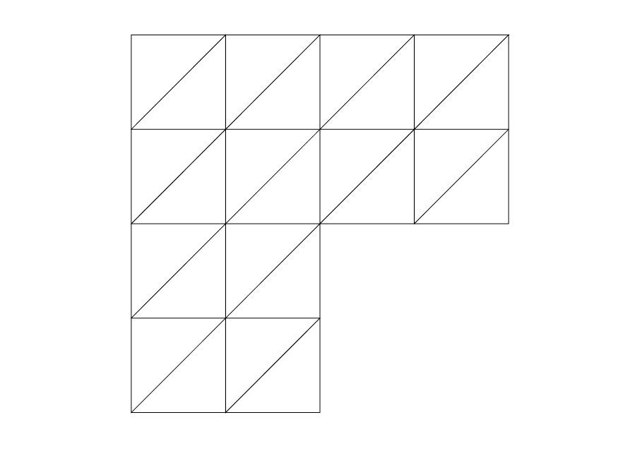
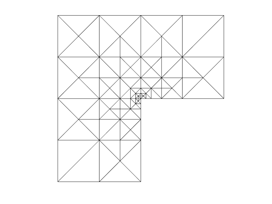
Figure 1. Left: initial uniform mesh; Right: $10$ times local refined mesh by bisection algorithm.

These limitations could reduce the efficiency of adaptive algorithms. We demonstrate these numerical performances explicitly in the following example.

Example 2.2.

In this example, we consider the following parabolic equation

$$\left\{\begin{aligned} u_{t}-\Delta u&=f,&\text{in }&\Omega\times(0,1],\\ u&=0,&\text{on }&\partial\Omega\times(0,1],\\ u(\mathbf{x},0)&=u_{0},&\text{in }&\Omega,\end{aligned}\right.$$ (6)

where $\Omega=[-1,1]^{2}$ and the exact solution is

$$u(x,y,t)=\exp(-500(x-0.3\cos(2\pi t))^{2})\exp(-500(y-0.3\sin(2\pi t))^{2}).$$

We apply Algorithm 1 to solve (6) with a fixed uniform time step $\tau=0.1$. Figure 2 shows the initial mesh and the adaptive meshes generated after the first time step. From the results, we observe the following: i) The mesh refinement algorithm successfully generates a locally refined mesh in regions where $u_{0}$ or $u(x,y,0.1)$ exhibit large gradients, though it requires 8 iterations of refinement. ii) Once the refinement step is complete, the coarsening step efficiently reduces the mesh resolution in regions where only $u_{0}$ has large gradients.

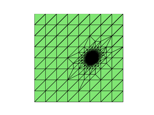
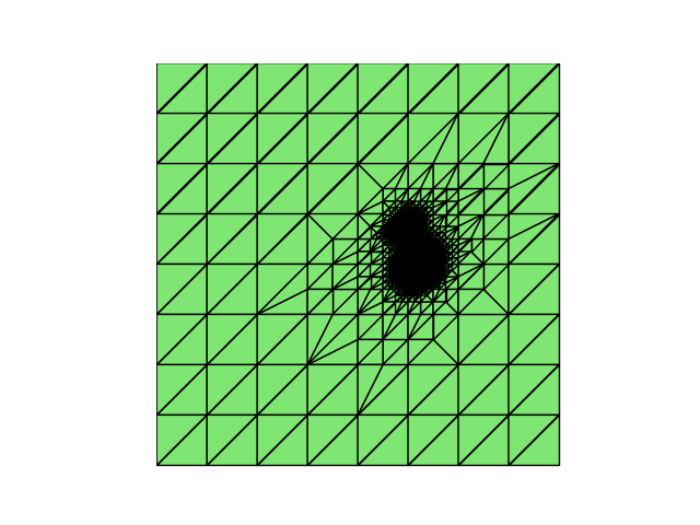
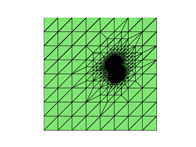
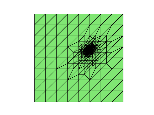
Figure 2. Example 2.2, adaptive meshes of Algorithm 1. Top left: final adaptive mesh at $t=0$; Top right: mesh after $4$ refinements at $t=0.1$; Bottom left: mesh after $8$ refinements at $t=0.1$; Bottom right: mesh after coarsen at $t=0.1$.

3. neural network-enhanced $hr$-AFEM

In the previous section, we identified the reasons behind the aforementioned limitations and demonstrated how the performance of the adaptive finite element algorithm can be inefficient in terms of overall computational costs. In this section, we discuss various methods to overcome the limitations of the standard $h$-adaptive finite element method and introduce a novel neural network-enhanced $hr$-AFEM.

To reduce the total number of adaptive iterations, we employ a mesh adaptation method capable of controlling the number of mesh vertices. In [36], Xiao et al. proposed an efficient adaptive finite element method for the elliptic equation, which leverages a gradient recovery technique and high-quality mesh optimization. A tailored adaptive strategy was developed to ensure that the adaptive computation process terminates within seven steps. In this work, we extend the mesh adaptation strategy in [36] to the adaptive finite element method for the parabolic equation (1). Note that many mesh generators, such as Gmsh, MeshLab, TetGen, and NETGEN, can produce high-quality meshes. For instance, Gmsh [14] allows users to refine meshes by providing a mesh size field as input, enabling control over approximation accuracy by adjusting mesh density. For simplicity, we employ Gmsh as the main tool to generate the mesh in this work.

Definition 3.1.

Given matrices $A,B\in\mathbb{R}^{m\times n}$ with elements $A_{ij}$ and $B_{ij}$, their Hadamard product is defined as:

$$A\odot B\in\mathbb{R}^{m\times n},\quad\text{with elements }(A\odot B)_{ij}=A_{ij}B_{ij}.$$

For any integer $s\geq 1$, the Hadamard power of $A$, denoted as $A^{\circ s}\in\mathbb{R}^{m\times n}$, is given by:

$$A^{\circ s}=\underbrace{A\odot A\odot\cdots\odot A}_{s\text{ times}},\quad\text{with elements }(A^{\circ s})_{ij}=A_{ij}^{s}.$$

Similarly, the Hadamard division is defined as:

$$A\oslash B\in\mathbb{R}^{m\times n},\quad\text{with elements }(A\oslash B)_{ij}=\frac{A_{ij}}{B_{ij}}.$$

Then we provide Algorithm 2 to generate such a mesh size field for Gmsh.

Input: Element error estimators $\{\eta_{h,K}\}$, element average edge size $\{h_{e}(K)\}$, iteration index $iteRO$, number of vertices $N_{v}$, number of elements $N_{K}$, dimension $d$, and mark ratio $\theta_{r}:=\{\text{number of marked vertices}\}/N_{v}$

Output: Mesh size field $Size$

1 Construct the sparse matrix $node2cell\in\mathbb{R}^{N_{v}\times N_{K}}$, where each row corresponds to a node and each column represents an element. The entry $(i,j)$ in this matrix is 1 if node $i$ belongs to element $j$, and 0 otherwise;

2 Compute the average edge length vector $h_{v}$ and error vector $E_{v}$ as follows:

$$h_{v}=\left(node2cell\cdot h_{e}(K)\right)\oslash(node2cell\cdot\mathbf{1}_{N_{K}\times 1}),$$

$$E_{v}=(node2cell\cdot\eta_{h,K})\oslash(node2cell\cdot\mathbf{1}_{N_{K}\times 1}),$$

where $\mathbf{1}_{N_{K}\times 1}$ is ones vector;

3 Compute node density vector $\rho$ by:

$$\rho=E_{v}^{\circ 2}\oslash h_{v}^{\circ d};$$

4 Find the smallest set $M=\{i_{1},i_{2},\cdots,i_{k}\}$ such that:

$$\sum_{i\in M}\rho[i]\geq\theta_{r}\sum_{i=1}^{N_{v}}\rho[i];$$

5 Define the scaling factor vector $Scale$ as follows:

$$Scale[i]=\begin{cases}1,&i\notin M,\\ \left(\sqrt[d]{1/2}\right)^{\log_{2}\left(N_{v}/k+1\right)},&i\in M;\end{cases}$$

Compute the mesh size field by

$$Size=h_{v}\odot Scale^{\circ\;iteRO}.$$

Algorithm 2 Mesh size field generator for Gmsh

The meshes generated by Gmsh with the user-specified size field are unstructured and non-nested, making the implementation of the interpolation $\Pi_{h}^{n}u_{h}^{n-1}$ in (S2) both challenging and less accurate. To address these difficulties, we employ neural networks to construct a mesh-free surrogate for $u_{h}^{n-1}$ instead of relying on the mesh-dependent interpolation $\Pi_{h}^{n}u_{h}^{n-1}$. Notably, the neural network is mesh-free and is trained only once, whereas the interpolation $\Pi_{h}^{n}u_{h}^{n-1}$, depending on the mesh, must be recomputed each time the mesh changes in an adaptive iteration.

Consider an $L$-layer neural network $u_{\theta}:\mathbb{R}^{d_{0}}\rightarrow\mathbb{R}^{d_{L}}$. At the $k$-th layer, an appropriate activation function $\sigma$ is applied component-wise, yielding

$$N^{(k)}(\mathbf{x}^{(k-1)}):=\sigma(\mathbf{W}_{k}\mathbf{x}^{(k-1)}+\mathbf{b}_{k}),$$

where $\mathbf{W}_{k}\in\mathbb{R}^{d_{k}\times d_{k-1}}$ is the $k$-th weight matrix and $\mathbf{b}_{k}\in\mathbb{R}^{d_{k}}$ is the $k$-th bias vector. In general, the activation function $\sigma$ can be arbitrary; however, we enforce a linear activation function in the output layer. This ensures that the neural network can effectively approximate the finite element solution, as certain activation functions have inherently bounded ranges. Therefore, the neural network $u_{\theta}$ is given by

$$u_{\theta}(\mathbf{x})=\mathbf{W}_{L}\left(N^{(L-1)}\circ\cdots\circ N^{(2)}\circ N^{(1)}(\mathbf{x})\right)+\mathbf{b}_{L}.$$ (7)

An important part of neural networks is the activation function. Here, we consider the hyperbolic tangent function

$$\sigma(x)=\tanh{x}=\frac{e^{x}-e^{-x}}{e^{x}+e^{-x}}.$$

Let $\theta=((\mathbf{W}_{0},\mathbf{b}_{0}),\cdots,(\mathbf{W}_{L},\mathbf{b}_{L}))$ represent all the trainable parameters. Given a function $u\in C^{0}(\Omega)$, we train the neural network $u_{\theta}(\mathbf{x})$ that approximates $u$ using the data $\{(\mathbf{x}_{i},u(\mathbf{x}_{i})\}_{i=1}^{m}$. The network parameters $\theta$ are optimized by minimizing the empirical loss function $\mathcal{L}(u_{\theta})$, defined as

$$\theta^{*}=arg\min\limits_{\theta\in\Theta}\mathcal{L}(u_{\theta}),\quad\mathcal{L}(u_{\theta}):=\frac{1}{m}\sum\limits_{i=1}^{m}(u_{\theta}(\mathbf{x}_{i})-u(\mathbf{x}_{i}))^{2},$$

where $\Theta$ is the feasible set consisting of the parameters and hyperparameters of the neural network.

We denote neural networks to find the mesh-free surrogate of the finite element solution $u_{h}^{n-1}$ by $u_{\theta}^{n-1}$, which is mesh-free, trained only one time, and initialized with the previous step optimizer. It eliminates the need to compute the projection $\Pi_{h}^{n}u_{h}^{n-1}$ in each adaptive iteration. To ensure $u_{\theta}^{n-1}$ satisfies the homogeneous Dirichlet boundary condition, we follow [28] and define

$$u_{\theta}^{n-1}(\mathbf{x})=d(\mathbf{x})u_{\theta}(\mathbf{x}),$$ (8)

where $u_{\theta}(\mathbf{x})$ is given by (7), and $d(\mathbf{x})$ is the distance function to the boundary of the domain $\Omega$, defined as

$$d(\mathbf{x}):=d(\mathbf{x},\partial\Omega)=\min\limits_{\mathbf{y}\in\partial\Omega}|\mathbf{x}-\mathbf{y}|.$$

Denote the set of vertices of $\mathcal{T}_{h}^{n-1}$ by $\mathcal{N}_{h}^{n-1}$, we define the loss function $L(u_{\theta}^{n-1};\mathcal{T}_{h}^{n-1})$ as

$$L(u_{\theta}^{n-1};\mathcal{T}_{h}^{n-1})=\frac{1}{\sharp\mathcal{N}_{h}^{n-1}}\sum_{\mathbf{x}\in\mathcal{N}_{h}^{n-1}}\left|u_{\theta}^{n-1}(\mathbf{x})-u_{h}^{n-1}(\mathbf{x})\right|^{2},$$ (9)

where $\sharp\mathcal{N}_{h}^{n-1}$ represents the number of vertices (NOV) in the mesh $\mathcal{T}_{h}^{n-1}$. We then find $u_{\theta^{*}}^{n-1}(\mathbf{x})=d(x)u_{\theta^{*}}(\mathbf{x})$ by solving $\theta^{*}=arg\min\limits_{\theta}L(u_{\theta}^{n-1};\mathcal{T}_{h}^{n-1})$, ensuring that the minimizer $u_{\theta^{*}}^{n-1}(\mathbf{x})$ is a good approximation of $u_{h}^{n-1}(\mathbf{x})$ and thus serves as a mesh-free surrogate for $u_{h}^{n-1}$ over the whole computational domain.

Remark 3.2.

For the parabolic equation with a nonhomogeneous Dirichlet boundary condition $u|_{\partial\Omega}=g$, we can modify the neural network in (8) as

$$u_{\theta}^{n-1}(\mathbf{x})=d(\mathbf{x})u_{\theta}(\mathbf{x})+h(\mathbf{x}),\qquad h(\mathbf{x})=\left\{\begin{aligned} g(\mathbf{x},t_{n-1}),&\quad x\in\partial\Omega,\\ 0,&\quad x\not\in\partial\Omega,\end{aligned}\right.$$

to make the neural network $u_{\theta}^{n-1}(\mathbf{x})$ satisfy the boundary conditions.

Remark 3.3.

Since the neural network $u_{\theta}^{n-1}$ is mesh-free, it needs to be trained only once for adaptive computations at the $n$-th time step, regardless of how many times the mesh is adjusted during the adaptation procedure. Furthermore, the adaptive algorithm utilizes the same neural network for all time steps, with the primary training effort focused on the initial step using a set of initialized neural network parameters. Instead of reinitializing the parameters at each time step, the network reuses the existing weights and biases from the previous step to fine-tune subsequent time steps, which can significantly save the training time. Our experiments demonstrate that achieving sufficient accuracy for each new time step requires only a few iterations and saves computational resources, with the loss converging to $10^{-6}$. As shown in Figure 4 in Section 4, the initial training may require several thousand iterations, whereas optimization for subsequent time steps typically takes around 100 iterations or fewer.

Based on the discussion above, given the approximation $u_{h}^{n-1}\in V_{h}^{n-1}$ at the time step $t_{n-1}$ and the selected error estimators, the computational process of the new adaptive algorithm for the parabolic equation (1) at the $n$-th time step is as follows:

Here, the SOLVE procedure has the form:

• choose the mesh $\mathcal{T}_{h}^{n}$ and corresponding finite element space $V_{h}^{n}$ at the time step $t_{n}$;

• solve the following equation to obtain the new approximation $u_{h}^{n}\in V_{h}^{n}$,

  $$(u_{h}^{n},v)+\tau(\nabla{u_{h}^{n}},\nabla v)=\tau\left(f_{h}^{n},v\right)+(u_{\theta^{*}}^{n-1},v),\qquad\forall v\in V_{h}^{n}.\$$ (10)

The accuracy of computing the term $(u_{\theta^{*}}^{n-1},v)$ in (10) directly impacts the accuracy of $u_{h}^{n}$. To generate a mesh at $t_{n}$ that accurately computes the term $(u_{\theta^{*}}^{n-1},v)$, it is essential to capture the singularities of $u_{\theta^{*}}^{n-1}$, are captured by the mesh $\mathcal{T}_{h}^{n-1}$. Therefore, we modify the error estimators in (5) as

$$\eta_{h,K}^{n}=\frac{\hat{\eta}_{h,K}^{n}+\hat{\eta}_{h,K}^{n-1}+|\hat{\eta}_{h,K}^{n}-\hat{\eta}_{h,K}^{n-1}|}{2},\qquad\eta_{h}^{n}=\left(\sum\limits_{K\in\mathcal{T}_{h}^{n}}\eta_{h,K}^{2}\right)^{1/2},$$ (11)

which combine the error estimates from both time levels and can guide the new mesh to capture the singularities at $t_{n}$ while ensuring accurate computation of the term $(u_{\theta^{*}}^{n-1},v)$.

In addition, to ensure the adaptive algorithm terminates within 7 iterations per time step, we adopt the mesh adaptation strategy from [36]: Starting from an initial uniform coarse mesh, the adaptive finite element method is first applied to solve (10) for 5 iterations. Based on the reliable data $\{(\eta_{h}^{n,i},N_{i})\}_{i=3}^{5}$, where $i$ represents the iteration and $N_{i}$ represents NOV of the mesh at the $i$th iteration, the least squares method is used to fit the functional relationship between the error estimator and the NOV:

$$\eta_{h}^{n}\approx cN^{-p}.$$

With the fitted parameters $(c,p)$, we determine the NOV required to satisfy $\eta_{h}^{n}\leq eTol$, given by

$$N=\left\lceil\sqrt[p]{c/eTol}\right\rceil,$$

which, together with the error estimators, necessitates the computation of the size field using Algorithm 2. We then generate the mesh $\mathcal{T}_{h}^{n}$ via Gmsh based on the computed size field and solve (10) on this mesh. A final adaptive process is performed to ensure that the finite element approximation meets the required accuracy.

Following this computational process, we present a neural network-enhanced $hr$-adaptive algorithm for the parabolic equation (1) in Algorithm 3.

Input: Domain $\Omega$, source term $f$, tolerance $eTol$, initial data $u_{0}$, time step $\tau$

Output: The meshes $\{\mathcal{T}_{h}^{n}\}_{n=1}^{N}$ and finite element approximations $\{u_{h}^{n}\}_{n=1}^{N}$

1 Generate an initial uniform mesh $\mathcal{T}_{h}^{initial}$ using Gmsh with a given mesh diameter;

2 Set $\mathcal{T}_{h}^{0}=\mathcal{T}_{h}^{initial}$, $t_{0}=0$;

3 for $k=1$ to $7$ do

4    (PROJECT) determine the number of the vertices $N_{k}$ in the mesh $\mathcal{T}_{h}^{0}$ and compute the projection $u_{h}^{0}=Pu_{0}$;

5    (ESTIMATE) compute the recovery-based error estimators $\{\eta_{h,K}^{0,k}\}$ and $\eta_{h}^{0,k}$;

6    if $\eta_{h}^{0,k}\leq eTol$ or $k==7$  then

7       break ;

8      

9   else

10       if $k==5$ then

11          Determine the parameters $(c,p)$ in $\eta_{h}^{0}=cN^{-p}$ by least square fitting with data $\{(\eta_{h}^{0,i},N_{i})\}_{i=3}^{5}$;

12          Calculate $N=\left\lceil\sqrt[p]{c/eTol}\right\rceil$;

13          Set $iteRO=\max\left(\left\lceil\log_{2}\left(\frac{N}{N_{k-1}}\right)\right\rceil,1\right)$ ;

14         

15      else

16          Set $iteRO=1$ ;

17         

18      

19   

20   (SIZING) compute the mesh size field $F_{0}$ by Algorithm 2 based on $\{\eta_{h,K}^{0,k}\}$ and $iteRO$;

21    (GENERATE) update the mesh $\mathcal{T}_{h}^{0}$ using Gmsh based on the mesh size field $F_{0}$.

22for $n=1$ to $N$  do

23    (LEARN) train a neural network $u_{\theta}^{n-1}$ to learn the finite element solution $u^{n-1}_{h}$, and obtain the minimizer as $u_{\theta^{*}}^{n-1}$;

24    Set $\mathcal{T}_{h}^{n}=\mathcal{T}_{h}^{initial}$, $t_{n}=t_{n-1}+\tau$;

25    for $k:=1$ to $7$ do

26       Determine the number of the vertices $N_{k}$ in the mesh $\mathcal{T}_{h}^{n}$;

27       (SOLVE) solve problem (10) for $u^{n}_{h}$ on $\mathcal{T}_{h}^{n}$ using the data $u_{\theta^{*}}^{n-1}$;

28       (ESTIMATE) compute the recovery-based error estimators $\{\eta_{h,K}^{n,k}\}$ and $\eta_{h}^{n,k}$;

29       if $\eta_{h}^{n,k}\leq eTol$ or $k==7$  then

30          break ;

31         

32      else

33          if $k==5$ then

34             Calculate the parameters $(c,p)$ in $\eta_{h}^{n}=cN^{-p}$ by least square fitting with data $\{(\eta_{h}^{n,i},N_{i})\}_{i=3}^{5}$ ;

35             Calculate $N=\left\lceil\sqrt[p]{c/eTol}\right\rceil$;

36             Set $iteRO=\max\left(\left\lceil\log_{2}\left(\frac{N}{N_{k-1}}\right)\right\rceil,1\right)$ ;

37            

38         else

39             Set $iteRO=1$ ;

40            

41         

42      

43      (SIZING) compute the mesh size field $F_{0}$ by Algorithm 2 based on the local error estimators $\{\eta_{h,K}^{n,k}\}$ and $iteRO$;

44       (GENERATE) update the mesh $\mathcal{T}_{h}^{n}$ using Gmsh based on the mesh size field $F_{n}$.

45   

Algorithm 3 Neural network-enhanced $hr$-AFEM for the parabolic equation (1)

To end this section, we give some remarks on the proposed neural network-enhanced $hr$-AFEM.

Remark 3.4.

In Algorithm 3, it is noteworthy that the same coarse initial mesh, $\mathcal{T}_{h}^{\text{initial}}$, is used for all time steps. This differs from the standard Algorithm 1, where the adaptively refined mesh $\mathcal{T}_{h}^{n-1}$ from the previous time step serves as the initial mesh. Such a configuration reduces the degrees of freedom in (10), thereby enhancing computational efficiency. By leveraging a posteriori error estimators to construct size fields for adaptive mesh refinement and employing Gmsh to generate high-quality locally refined meshes, we ensure high accuracy of finite element solutions, superconvergence of gradient recovery, and the asymptotic exactness of the corresponding gradient recovery-based a posteriori error estimator.

Remark 3.5.

The combined estimator $\eta_{h}^{n}$ in (11) plays a crucial role in guiding the size field calculation in Algorithm 2 by incorporating error information from both time steps $t_{n}$ and $t_{n-1}$. To demonstrate this, we apply Algorithm 3 to solve (6) using the error estimator (11) with a relatively large time step of $0.1$. Figure 3 presents the final adaptive mesh at the initial step $t=0$ and a series of meshes generated by the adaptive algorithm during the time step at $t=0.1$. It can be observed that the adaptive algorithm terminates after $7$ iterations. Starting from a uniform coarse mesh, the nodes of the adaptive mesh, guided by the error estimator, concentrate in regions where the gradients of $u_{h}^{0}$ and $u_{h}^{1}$ are large.

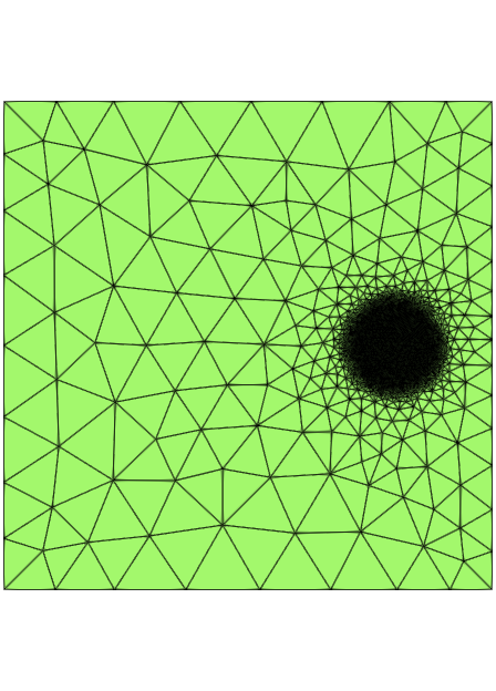
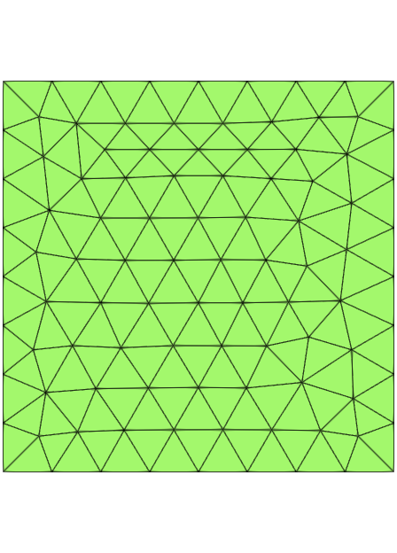
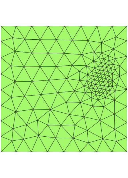
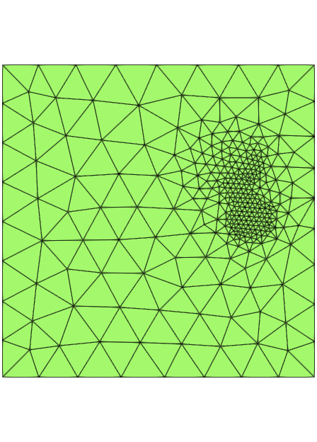
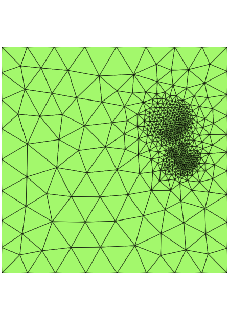
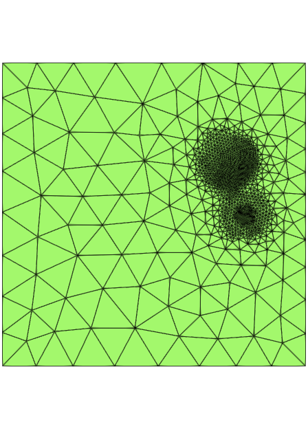
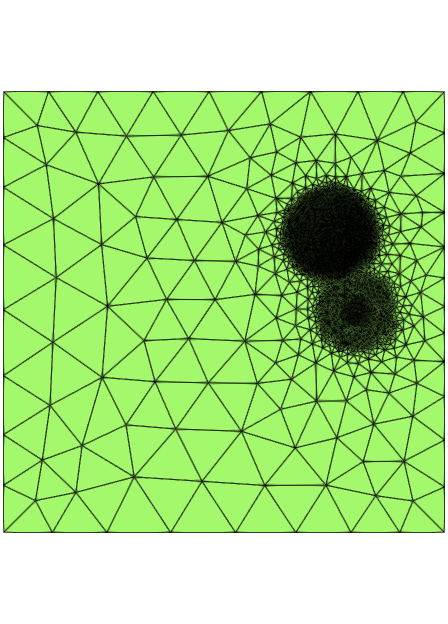
Figure 3. Example 2.2. Top left: final adaptive mesh at $t=0$; Top second left: initial mesh at $t=0.1$; Top third left to bottom right: adaptive meshes after one to six iterations at time step $t=0.1$.

4. Numerical Examples

In this section, we present numerical experiments to demonstrate the efficiency of the $hr$ adaptive Algorithm 3 in solving the parabolic equation in both 2D and 3D. These experiments are designed to evaluate the algorithm’s performance in handling dynamic singularities in the solutions. We focus on three primary test cases, each involving a different type of singularity with distinct behaviors:

• Rotation: A singularity rotates around the center of the domain, following a circular path while maintaining a constant amplitude.

• Diffusion: A singularity appears as a ring that either expands or contracts, changing in size and position over time, while its amplitude remains unchanged.

• Splitting: singularity initially appears as a single peak, which then splits into two symmetrical peaks moving away from the center. The amplitude of the original peak is evenly distributed between the two newly formed peaks.

In the following examples, unless stated otherwise, the conforming linear finite element is used in all numerical experiments, with the time step $\tau=0.01$. For the neural network training, the Adam optimizer is employed to minimize the loss function (9) to $10^{-6}$ with a learning rate of $0.001$, followed by the L-BFGS optimizer to ensure convergence (stagnation).

4.1. 2D Example

In this subsection, we present three 2D examples to verify the performance of the new adaptive Algorithm 3. For the computations, the iteration tolerance $eTol=0.01$, which primarily affects the computation of $iteRO$ in the fifth iteration and determines whether a sixth iteration is necessary. We consider the neural network (8) with the architecture $[2,40,40,40,1]$ consisting of two input neurons for $x$ and $y$, four hidden layers with $40$ neurons each, and a single output neuron. The weights are initialized using the Kaiming method, while the biases are set to zero. The $\tanh$ function is used as the activation function for all layers except the output layer, which has a linear activation function and no bias term ($b_{L}=0$).

Example 4.1.

(Rotation) Consider the 2D parabolic equation (1) in the domain $\Omega=[-1,1]^{2}$, with a source function $f$ chosen such that the exact solution $u$ is

$$u(x,y,t)=\exp\big{(}-500(x-0.3\cos(2\pi t))^{2}\big{)}\exp\big{(}-500(y-0.3\sin(2\pi t))^{2}\big{)}.$$

Figure 4 illustrates the number of neural network training iterations when reusing the weights and biases from the previous step at each time level. Approximately 25 epochs for Adam and 100 epochs for L-BFGS are needed at each time step.

In Figure 5, the top-left picture shows the initial uniform mesh, which also serves as the initial mesh for adaptive iterations at each time step. The next five pictures show the refined meshes over five successive refinements, with the process terminating before the sixth refinement as the tolerance $eTol=0.01$ is larger than the global error estimator. Mesh optimization through point addition or removal is essential for improving mesh quality, leading to approximately double the NOV at each step after the initial mesh generation, with values of 98, 180, 340, 681, 1388, and 12818, respectively. Since the NOV of the mesh generated by Algorithm 3 at the fifth step are significantly larger than those of the previous mesh, the global error estimator is generally smaller than the tolerance $eTol$, causing the termination of the algorithm before the sixth refinement.

Figure 6 illustrates the evolution of the numerical solutions and the corresponding mesh at different time steps. The mesh dynamically refines around sharp gradients or singularities, efficiently allocating resources where needed, and reveals a peak rotating around the coordinate origin. Notably, the grids shown here differ significantly from those in Figure 3 due to the smaller time step used, which causes the positions of two distinct singularities at adjacent time steps to nearly overlap.

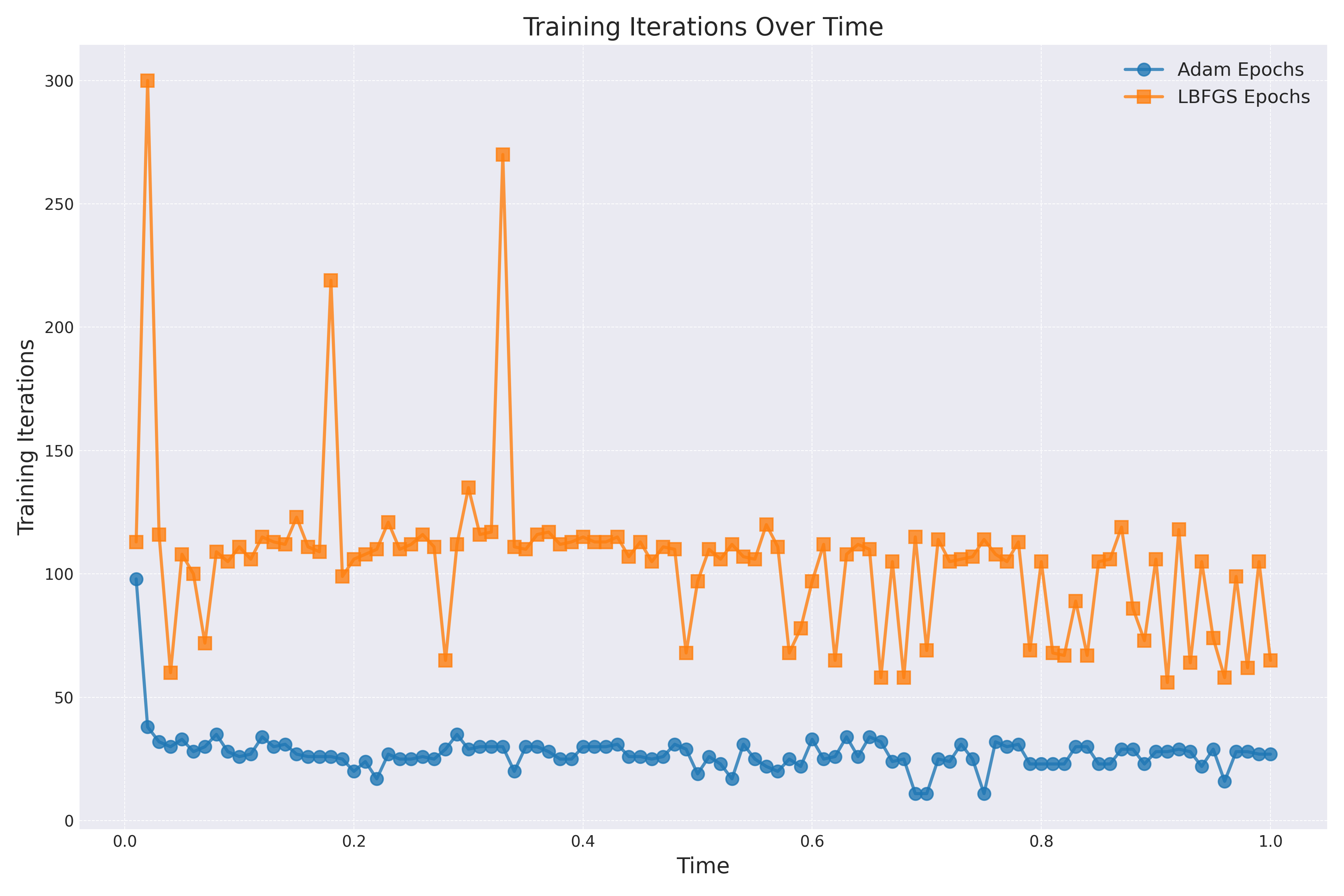
Figure 4. Example 4.1, training epochs at each time step.

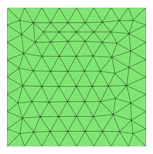
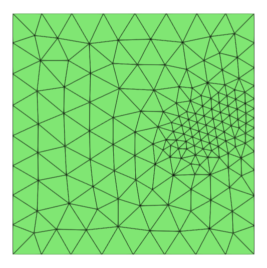
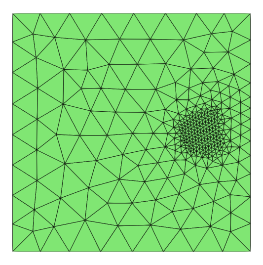
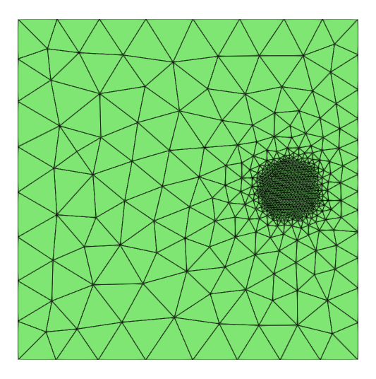
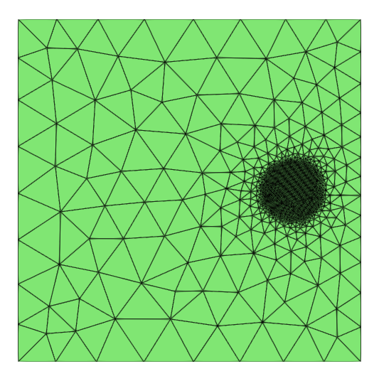
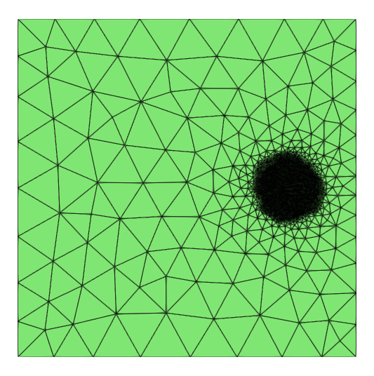
Figure 5. Example 4.1, initial mesh (top left) and its evolution through five adaptive refinements at $t=0.0$.

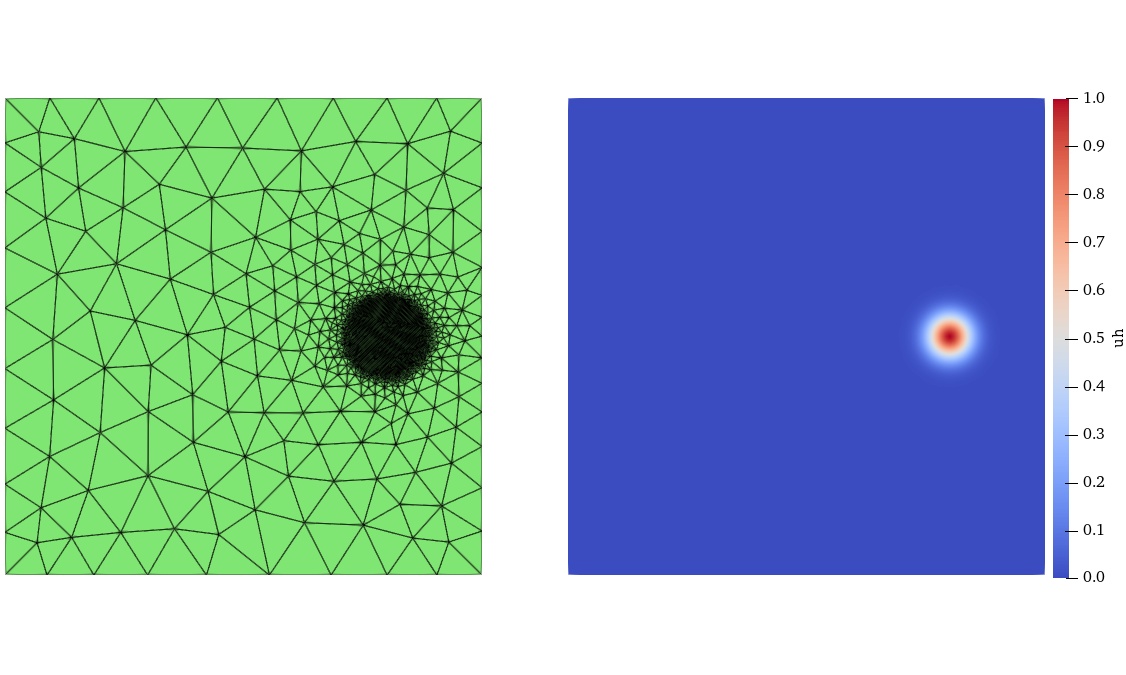
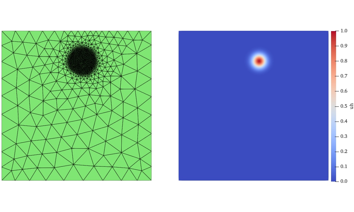
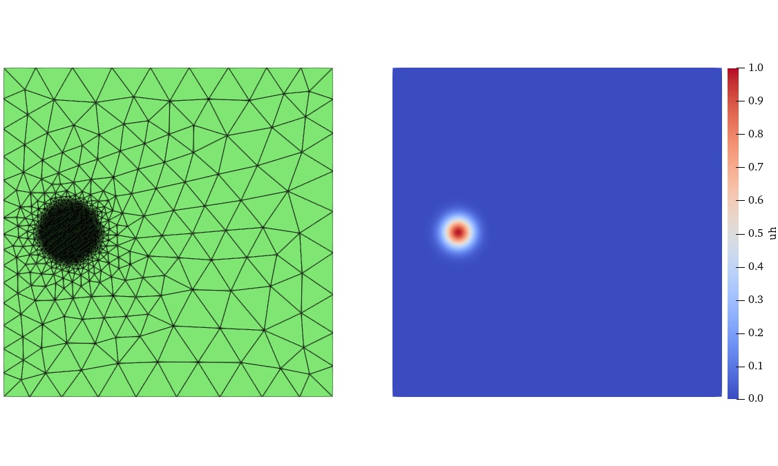
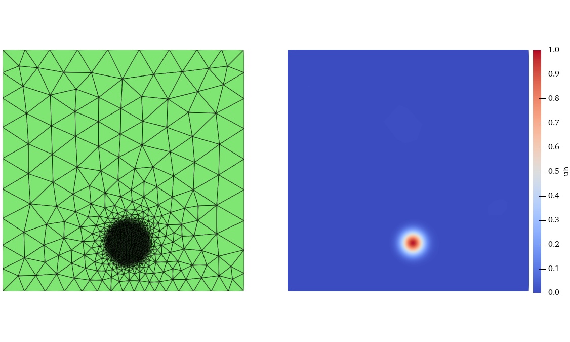
Figure 6. Example 4.1, snapshots of numerical solutions along with their corresponding adaptive meshes at 0.00, 0.25, 0.50, and 0.75 time.

Example 4.2.

(Diffusion) Consider the 2D parabolic equation (1) in the domain $\Omega=[-1,1]^{2}$, with the source function $f$ such that the exact solution $u$ is given by:

$$u(x,y,t)=\exp(-5000(\sqrt{x^{2}+y^{2}}+0.3t-0.4)^{2}).$$

In this example, the settings are the same as Example 4.1, except for the tolerance $eTol=0.05$. Similarly, Figure 7 illustrates the adaptive refinement process of the initial mesh over six iterations. The NOV at each iteration are 556, 1088, 2182, 4436, 9069, 18678, and 38659, respectively. Unlike the previous example, the NOV of the sixth mesh is twice that of the fifth mesh. Moreover, the need for a seventh mesh indicates that the error estimator obtained on the sixth mesh is still larger than the tolerance. This suggests that the mesh generated by the previous refinement did not meet the desired tolerance, even though the tolerance was used when calculating the NOV for the sixth mesh. This implies the necessity of one extra step after the least square fitting, namely the case $k==5$ in Algorithm 3. Four different time steps are shown in Figure 8, where the mesh and numerical solutions illustrate a scenario in which a ring-shaped crater gradually decreases its radius over time.

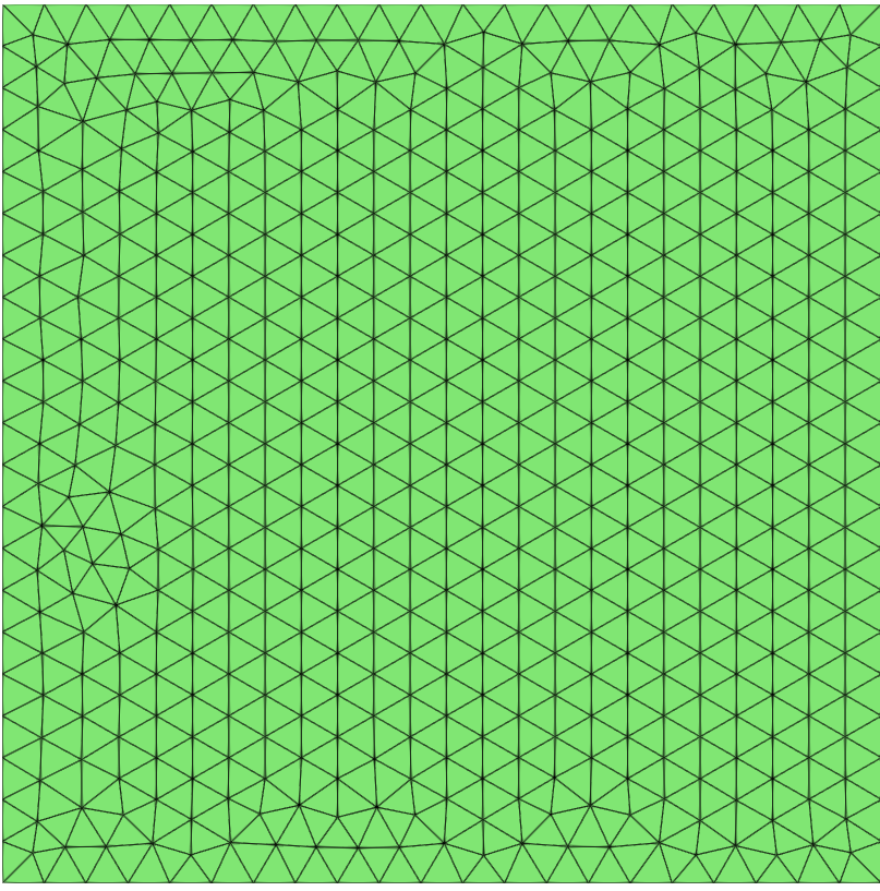
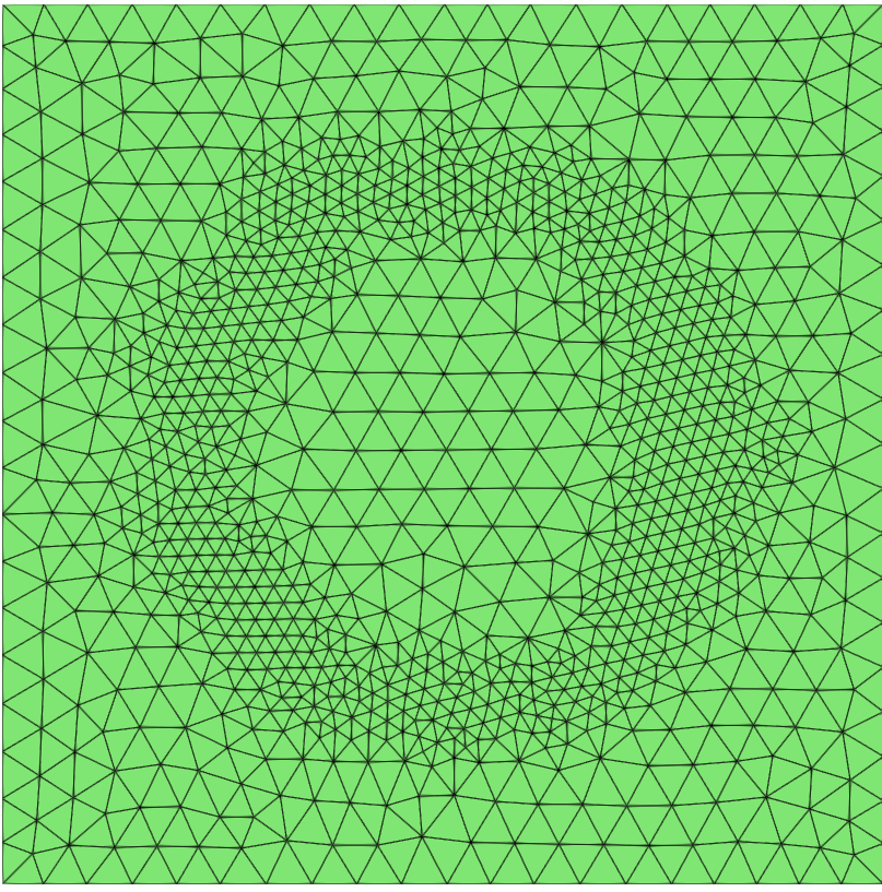
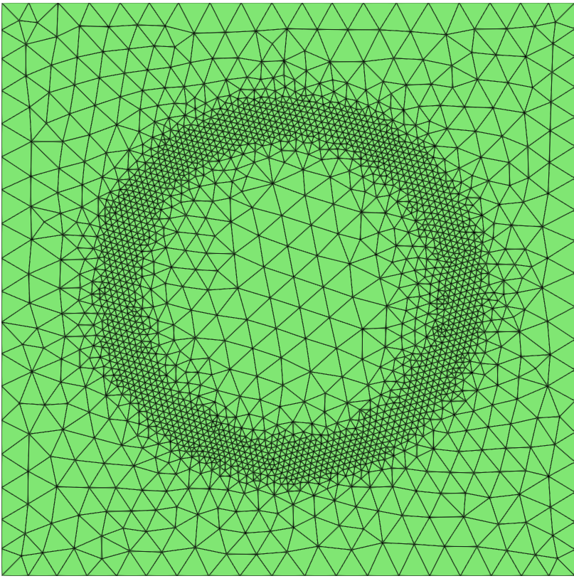
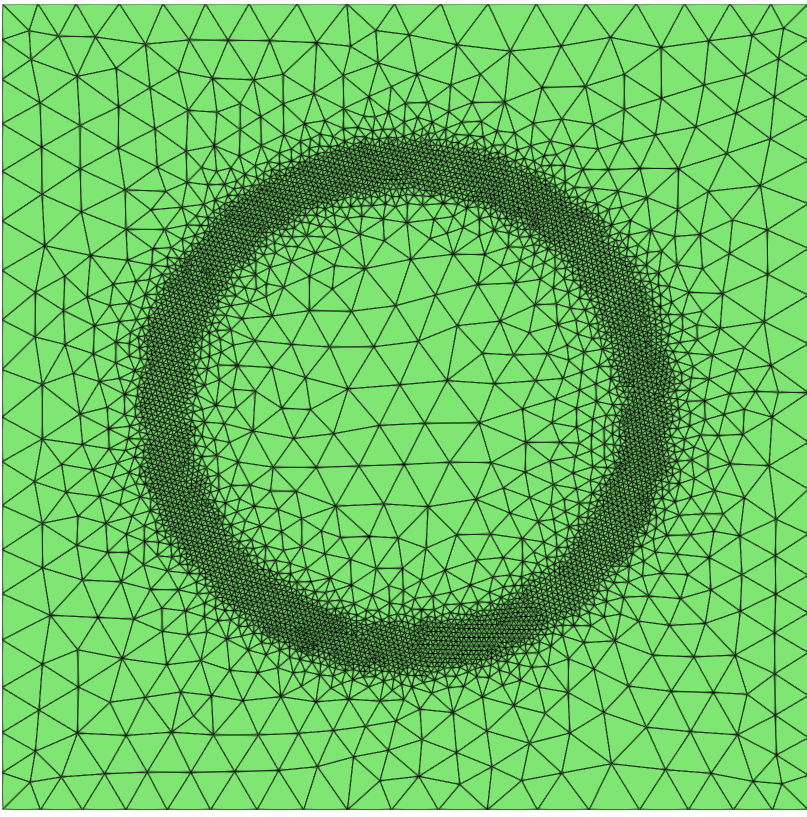
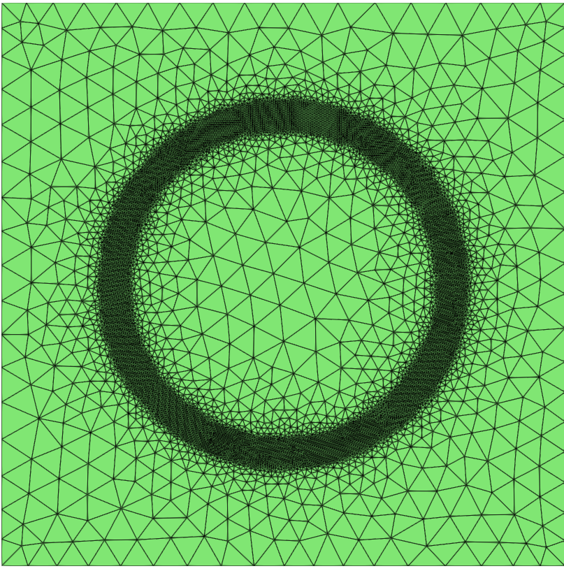
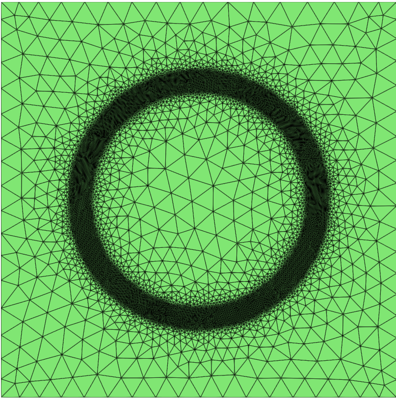
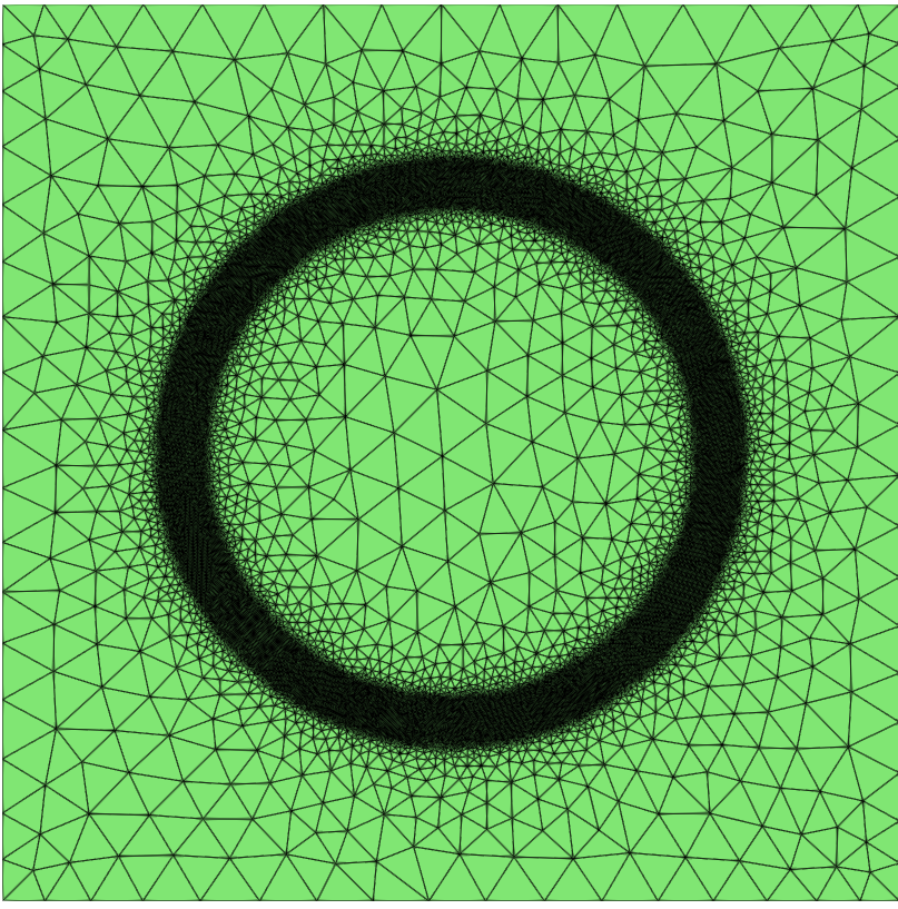
Figure 7. Example 4.2, initial mesh (left) and its evolution through six adaptive refinements at $t=0.0$.

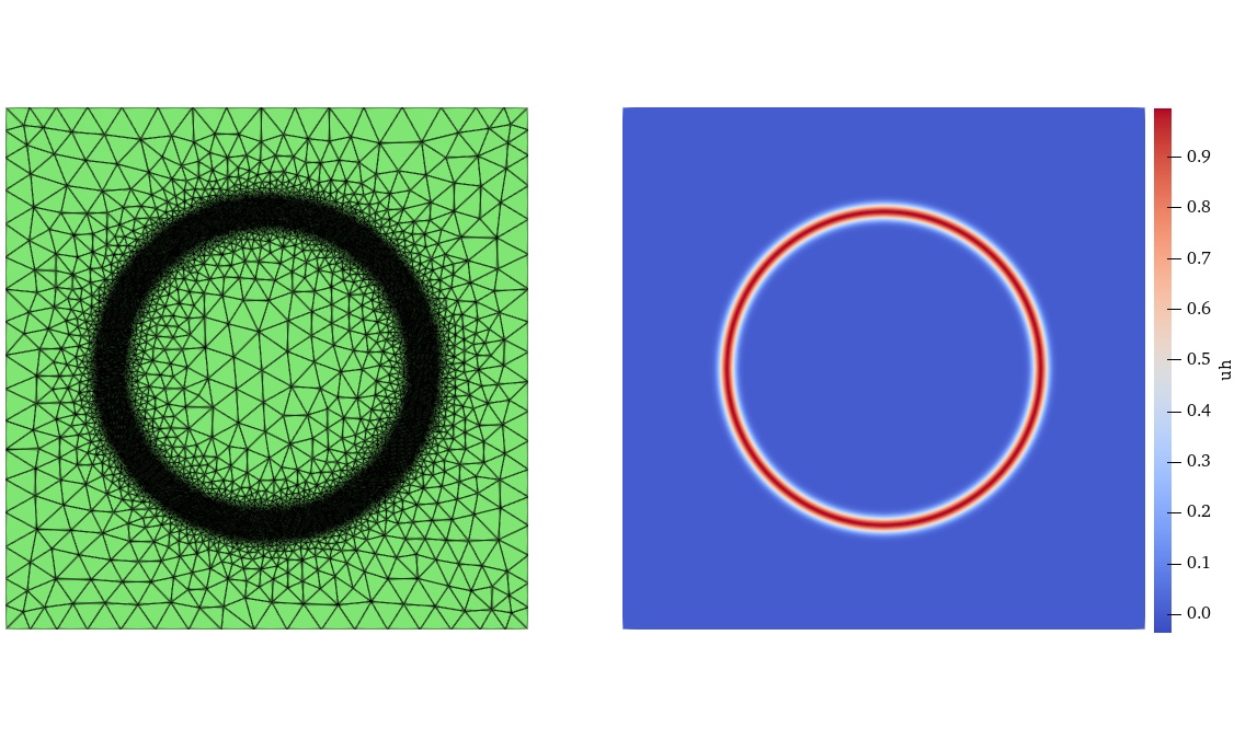
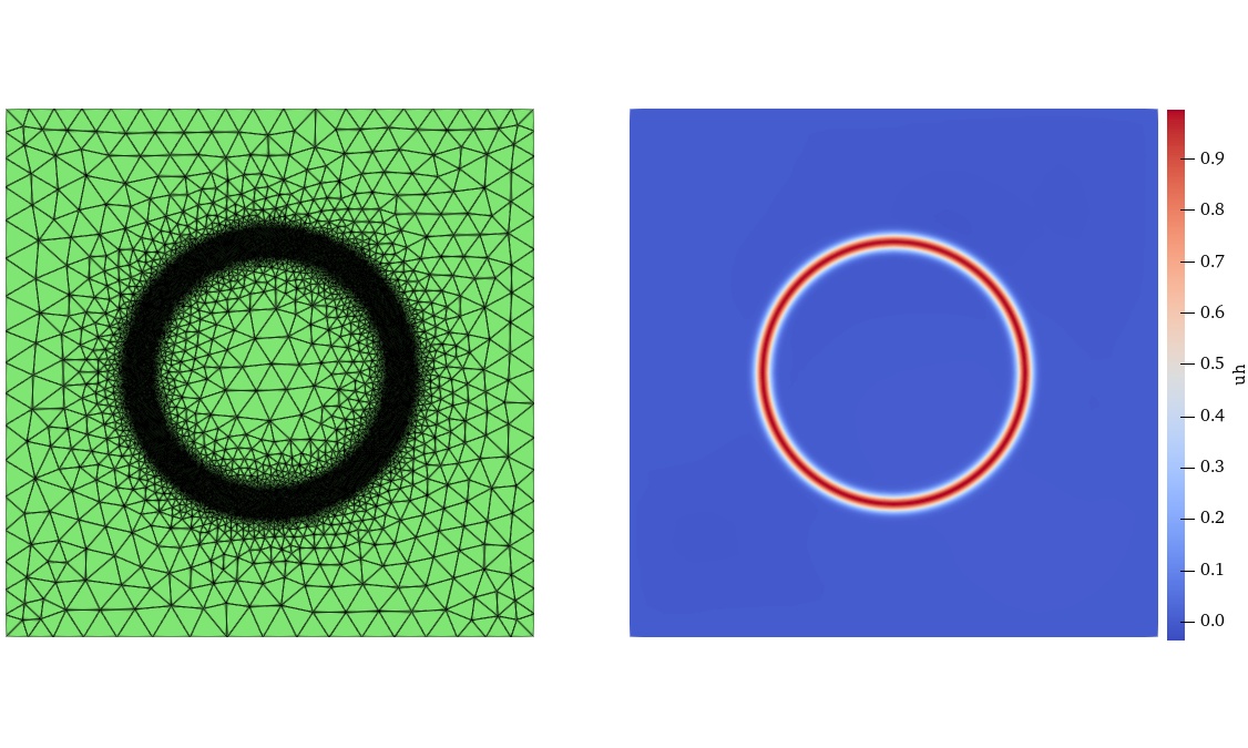
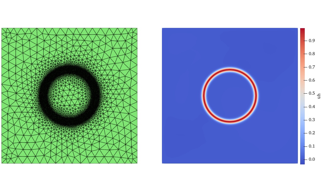
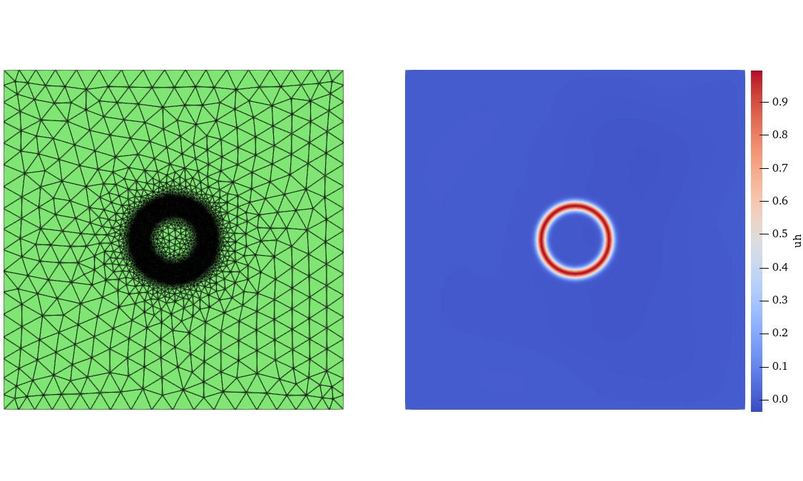
Figure 8. Example 4.2, snapshots of numerical solutions along with their corresponding adaptive meshes at 0.00, 0.25, 0.50, and 0.75 time.

Example 4.3.

(Splitting) Consider the 2D parabolic equation (1) in the domain $\Omega=[-1,1]^{2}$, with the source function $f$ such that the exact solution $u$ is given by:

$$u(x,y,t)=\exp(-300((x-0.3t)^{2}+y^{2}))+\exp(-300((x+0.3t)^{2}+y^{2})).$$

Consistent with Example 4.1, the computational settings remain unchanged with the tolerance $eTol=0.01$. Figure 9 shows the adaptive process of the initial mesh over six iterations, with the NOV at each iteration being 118, 206, 401, 813, 1677, and 3463, respectively. Figure 10 shows the evolution of the numerical solutions and the corresponding mesh at four different time steps. The refinement process dynamically captures the splitting of the central peak into two distinct moving peaks, maintaining a coarser resolution in smoother regions while ensuring high resolution in areas with sharp gradients.

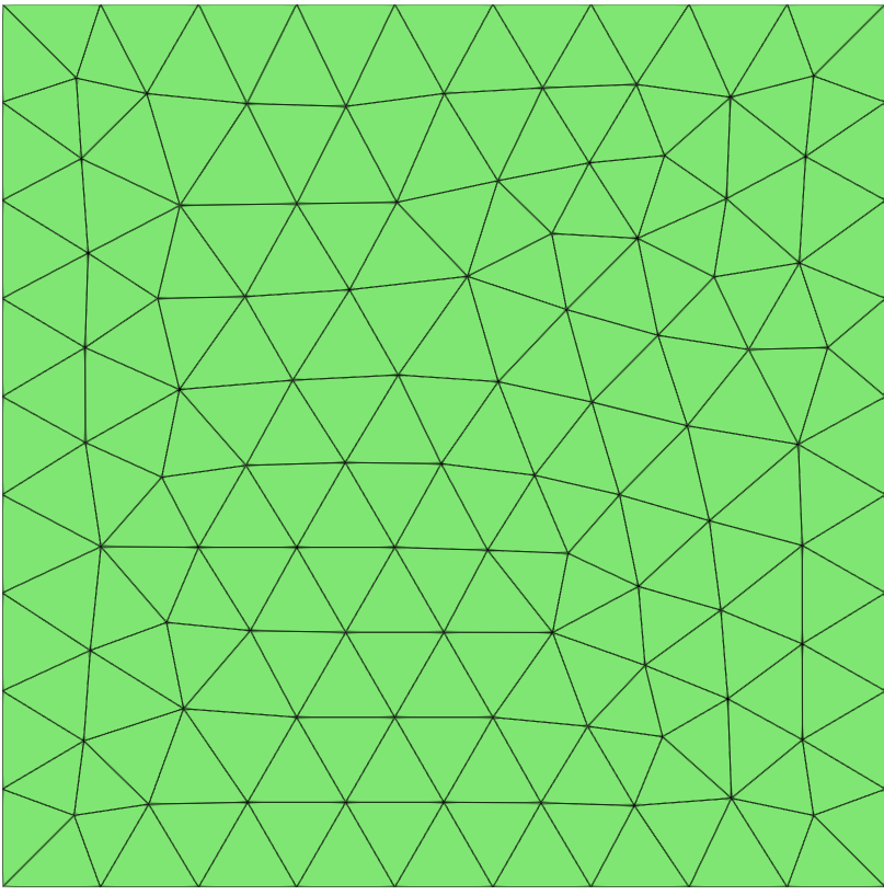
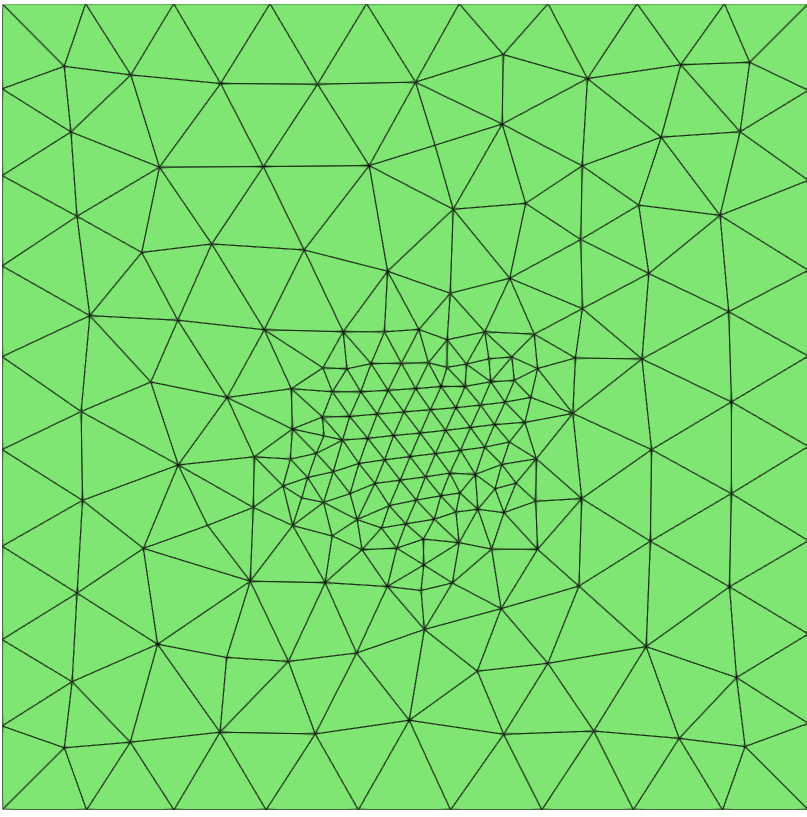
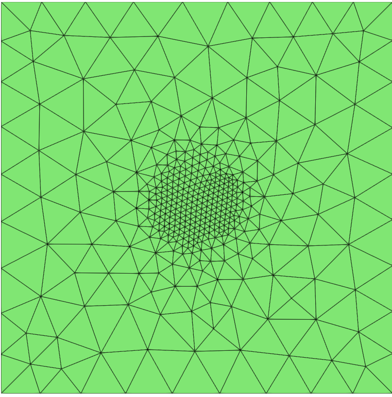
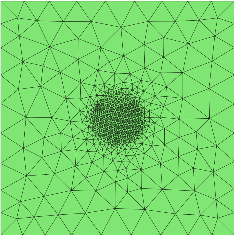
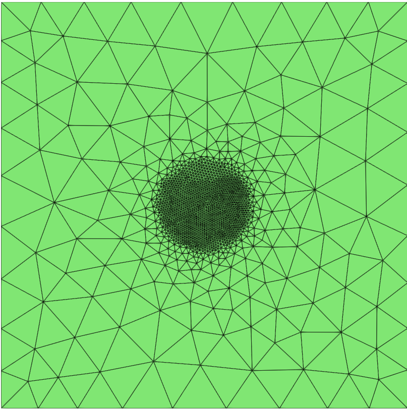
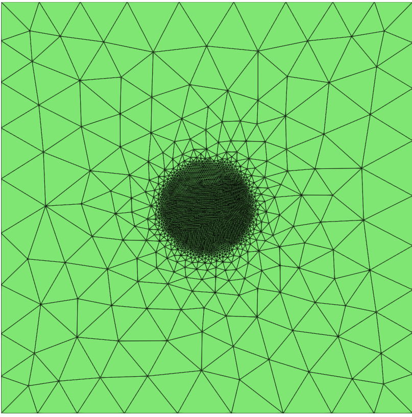
Figure 9. Example 4.3, initial mesh (top left) and its evolution through five adaptive refinements at $t=0.0$.

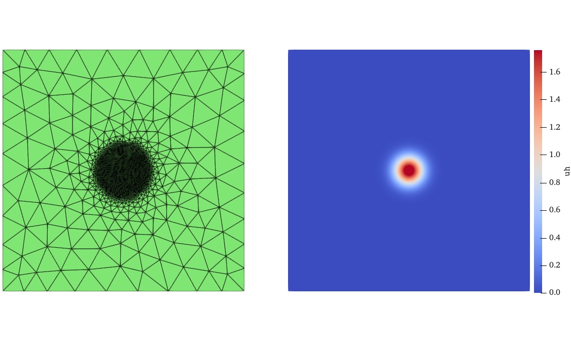
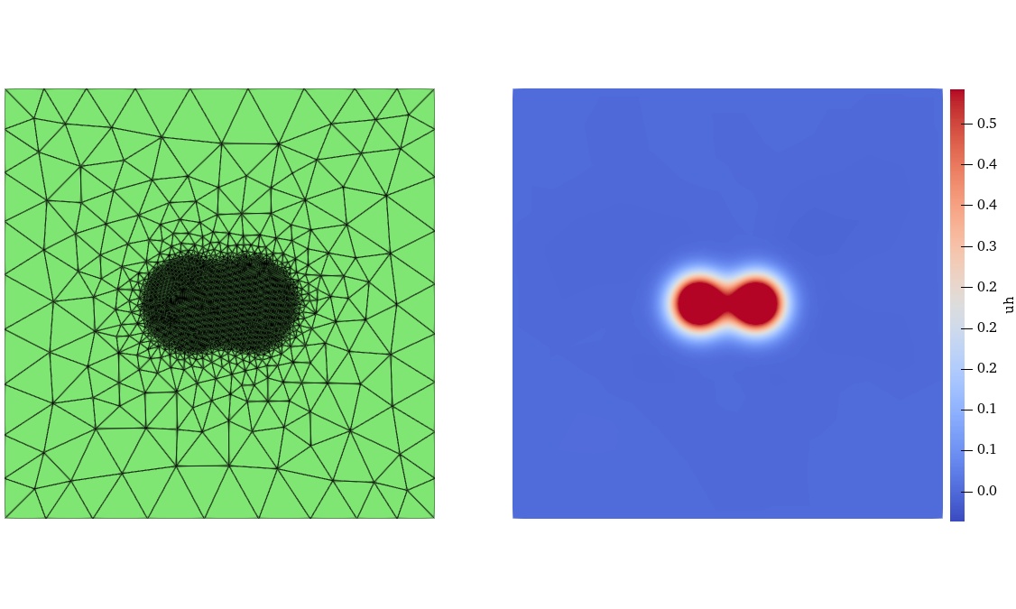
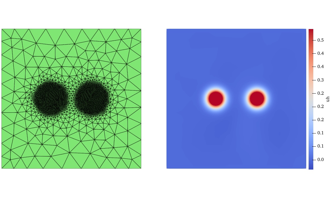
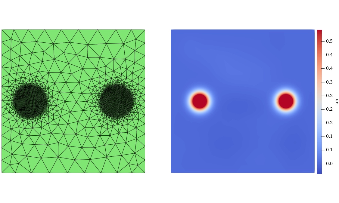
Figure 10. Example 4.3, snapshots of numerical solutions along with their corresponding adaptive meshes at 0.00, 0.25, 0.50, and 0.75 time.

4.2. 3D Example

In this subsection, we present three 3D numerical examples to demonstrate the efficiency and robustness of our proposed Algorithm 3. The only modification required compared to the previous section is the neural network configuration, which is updated to [3, 32, 32, 32, 32, 1], where the input nodes correspond to the spatial coordinates $x,y$ and $z$.

Example 4.4.

(Rotation) Consider the 3D parabolic equation (1) in the domain $\Omega=[-1,1]^{3}$, with the source function $f$ such that the exact solution $u$ is given by:

$$u(x,y,z,t)=\exp(-500(x-0.3\cos(2\pi t))^{2})\exp(-500(y-0.3\sin(2\pi t))^{2})\exp(-500z^{2}).$$

Apply Algorithm 3 with $eTol=0.1$. Figure 11 illustrates the mesh refinement process at initial time $t=0.0$, showing the transition from an initial uniform mesh to its evolution over five refinement steps. The NOV at each iteration are 944, 1685, 2819, 4827, 8733, and 15908, respectively. Figure 12 presents the numerical results and corresponding meshes at four different time instances, demonstrating the adaptive method’s capability to efficiently handle time-dependent 3D problems with high precision.

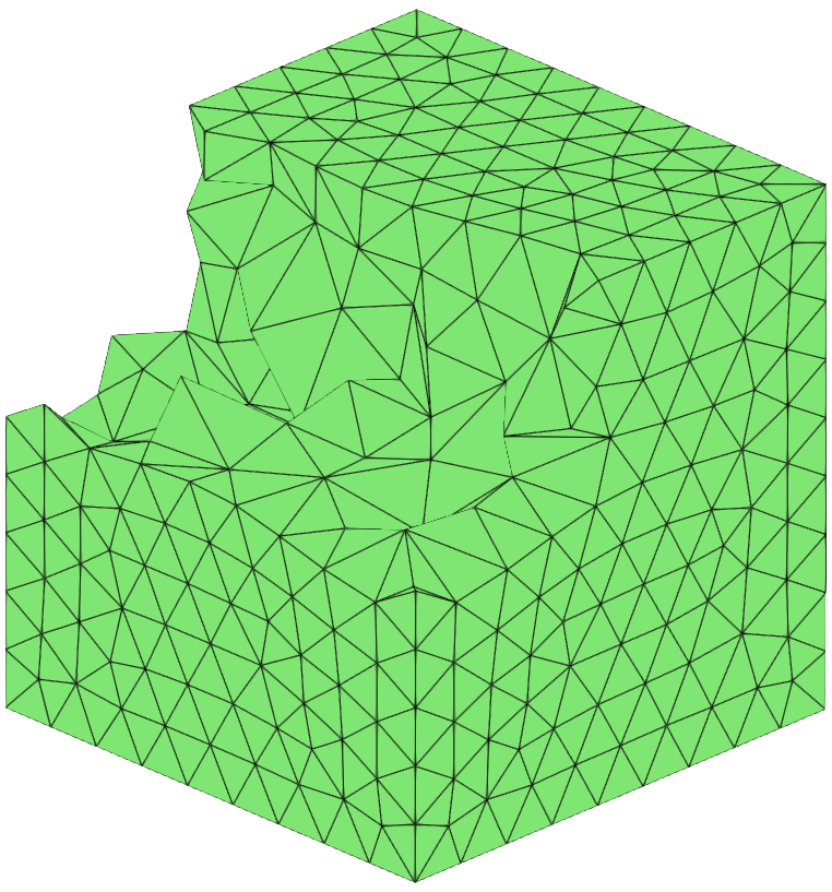
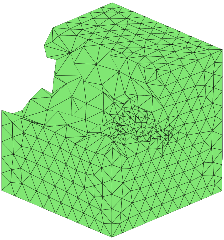
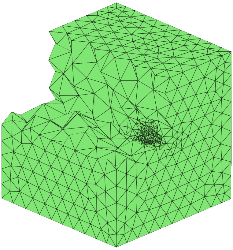
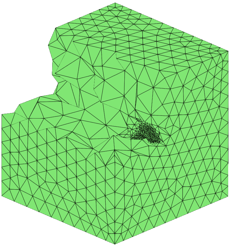
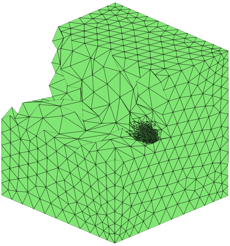
Figure 11. Example 4.4, initial mesh (top left) and its evolution through five adaptive refinements at $t=0.0$.

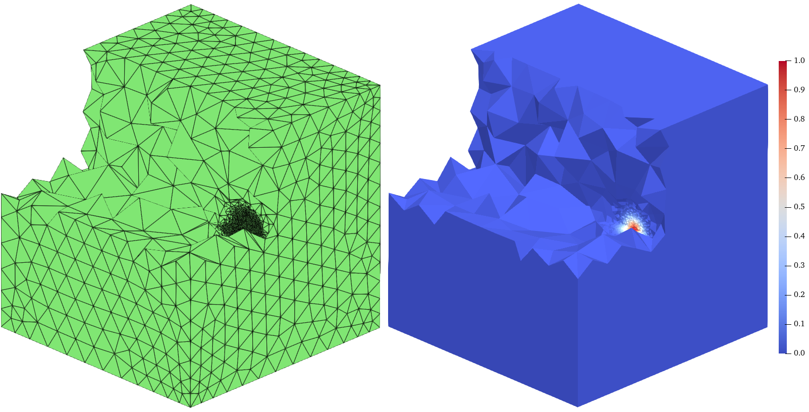
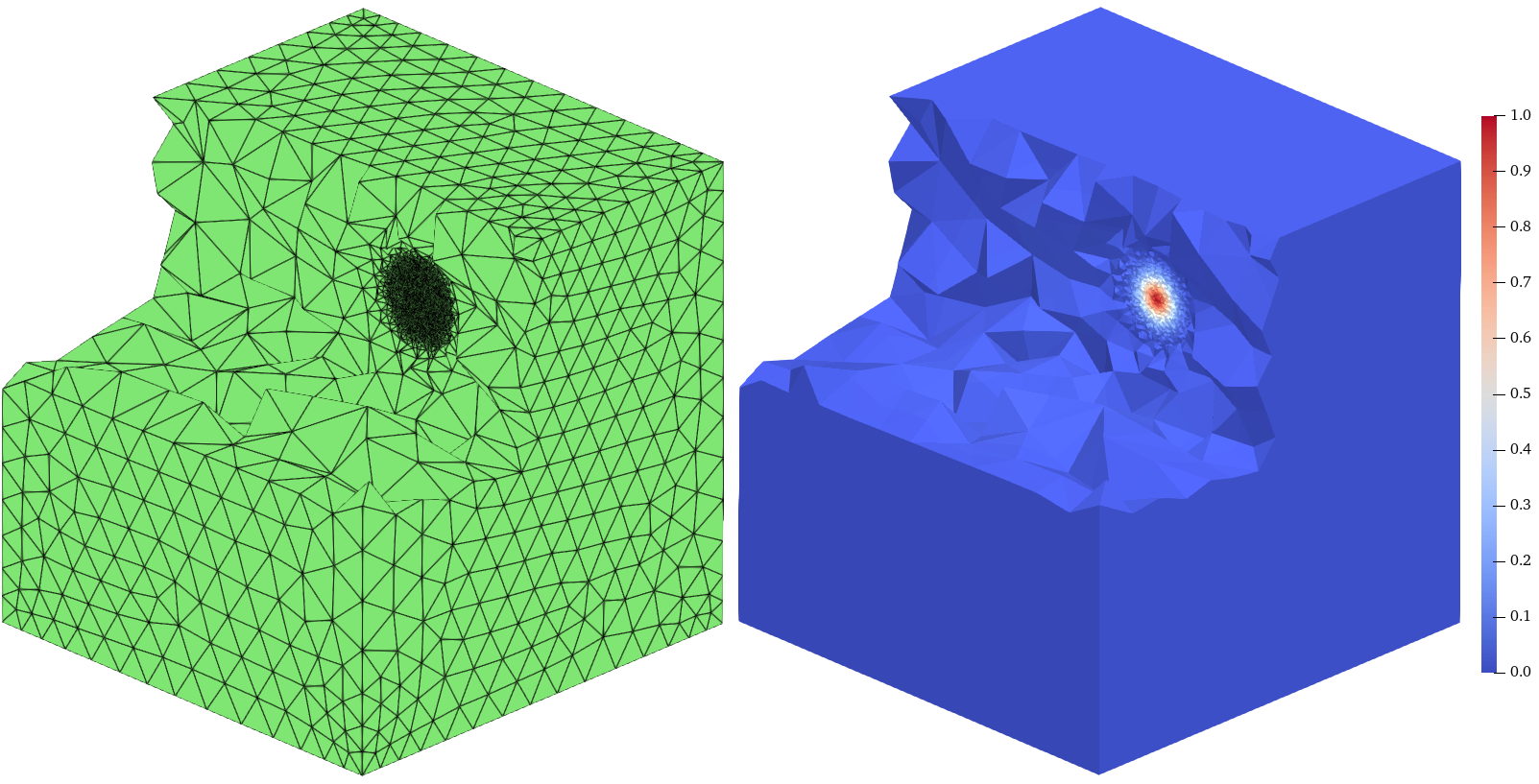
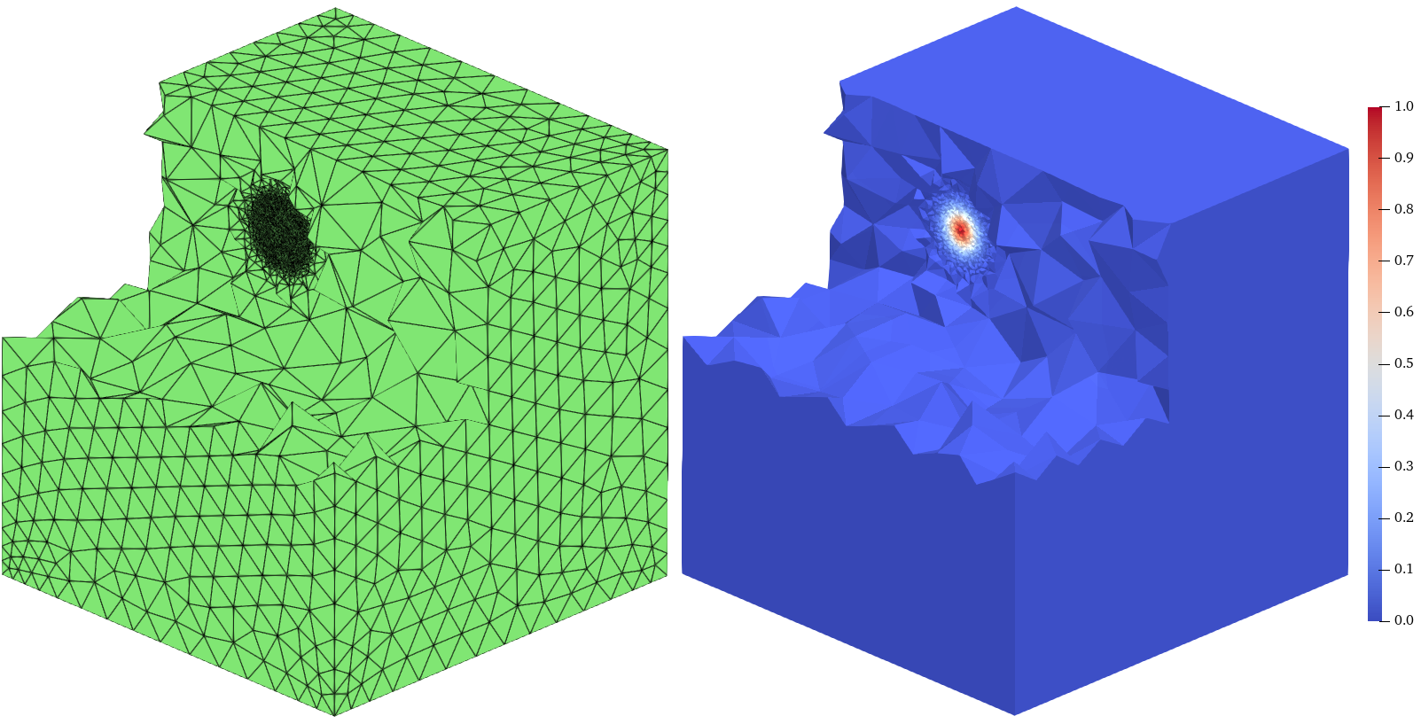
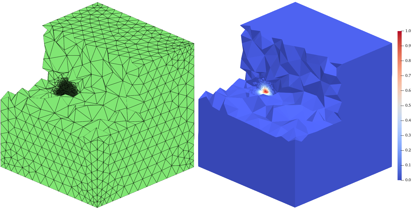
Figure 12. Example 4.4, snapshots of numerical solutions along with their corresponding adaptive meshes at 0.00, 0.17, 0.34, and 0.50 time.

Example 4.5.

(Diffusion) Consider the 3D parabolic equation (1) in the domain $\Omega=[-1,1]^{3}$, with the source function $f$ such that the exact solution $u$ is given by:

$$u(x,y,z,t)=\exp(-5000(\sqrt{x^{2}+y^{2}+z^{2}}+0.3t-0.4)^{2}).$$

We set the mesh refinement tolerance $eTol=0.4$, causing the adaptive algorithm to terminate early before reaching the least squares fitting step, as the tolerance condition is met. Nevertheless, the algorithm remains effective despite the early termination. Figure 13 illustrates the adaptive process of the initial mesh over four refinements, listing the NOV at each iteration as 8080, 14502, 27327, 56739, and 128527, respectively. Figure 14 presents the evolution of the numerical solutions and corresponding meshes at four distinct time points, with refinement specifically focusing on the contracting spherical shell.

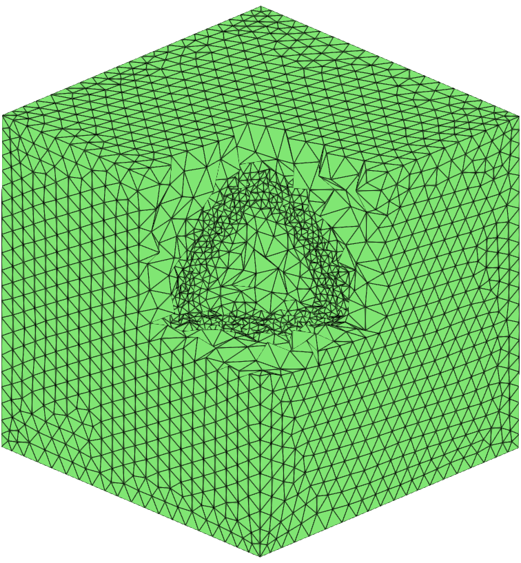
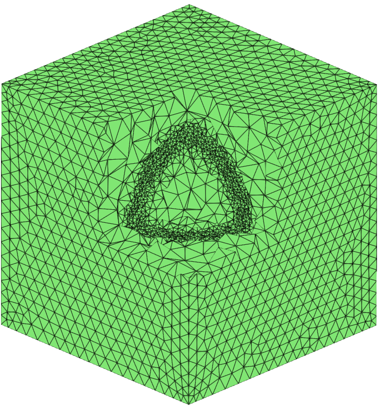
Figure 13. Example 4.5, initial mesh (left) and its evolution through four adaptive refinements at $t=0.0$.

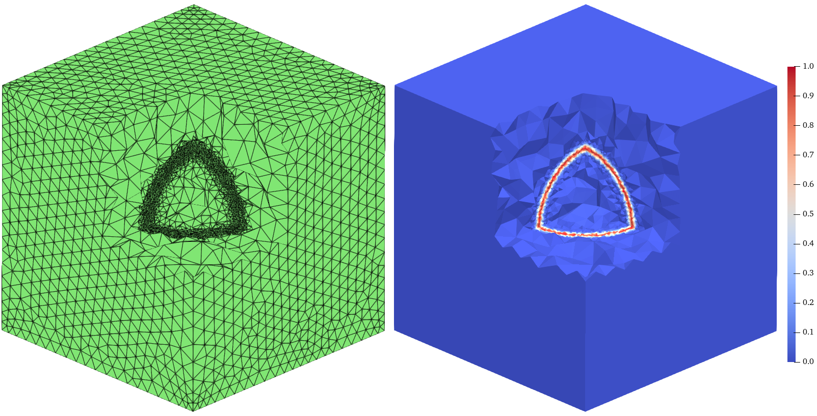
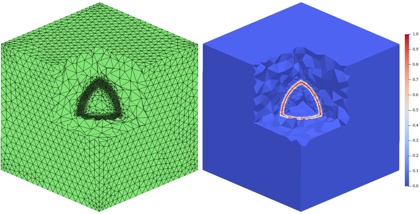
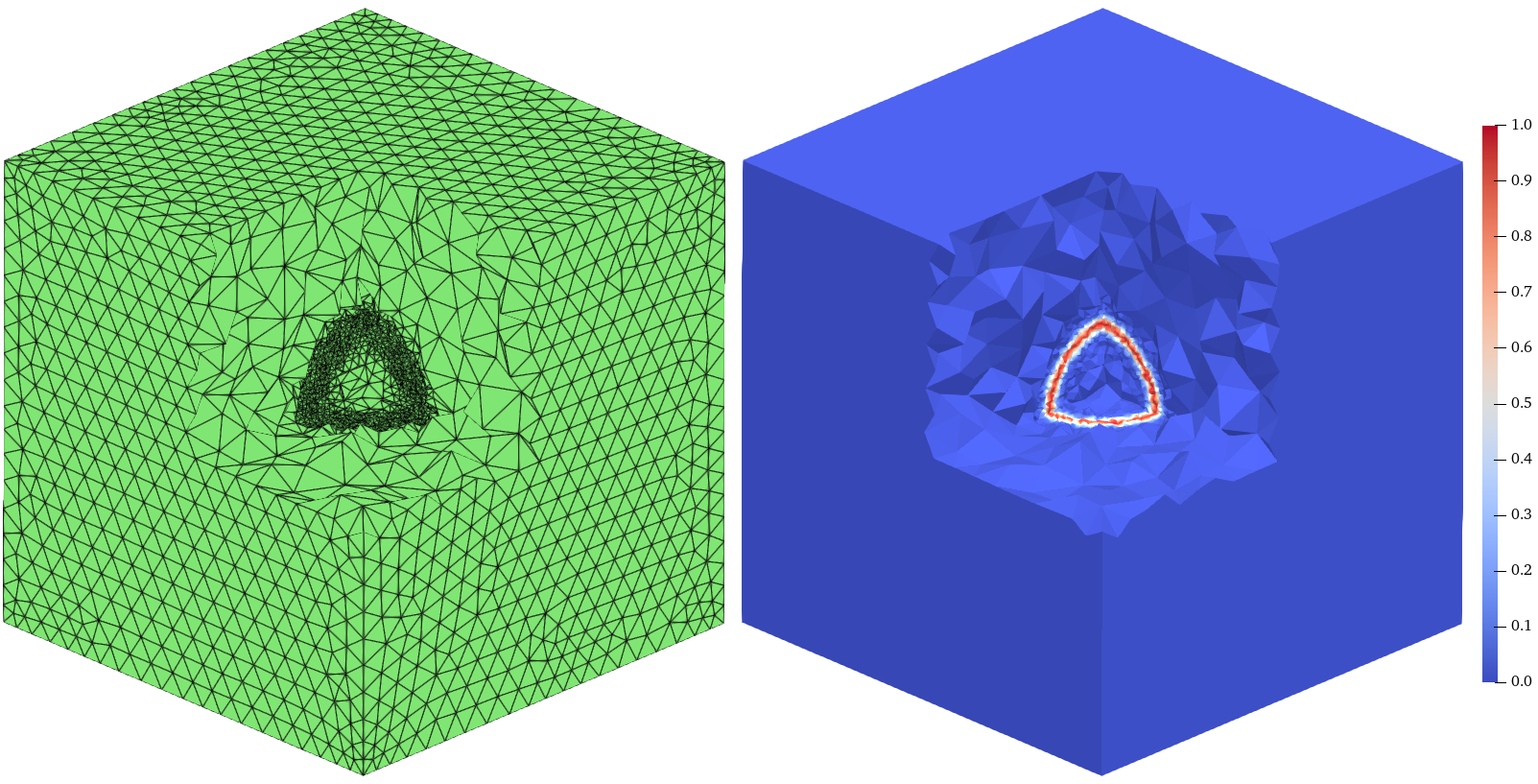
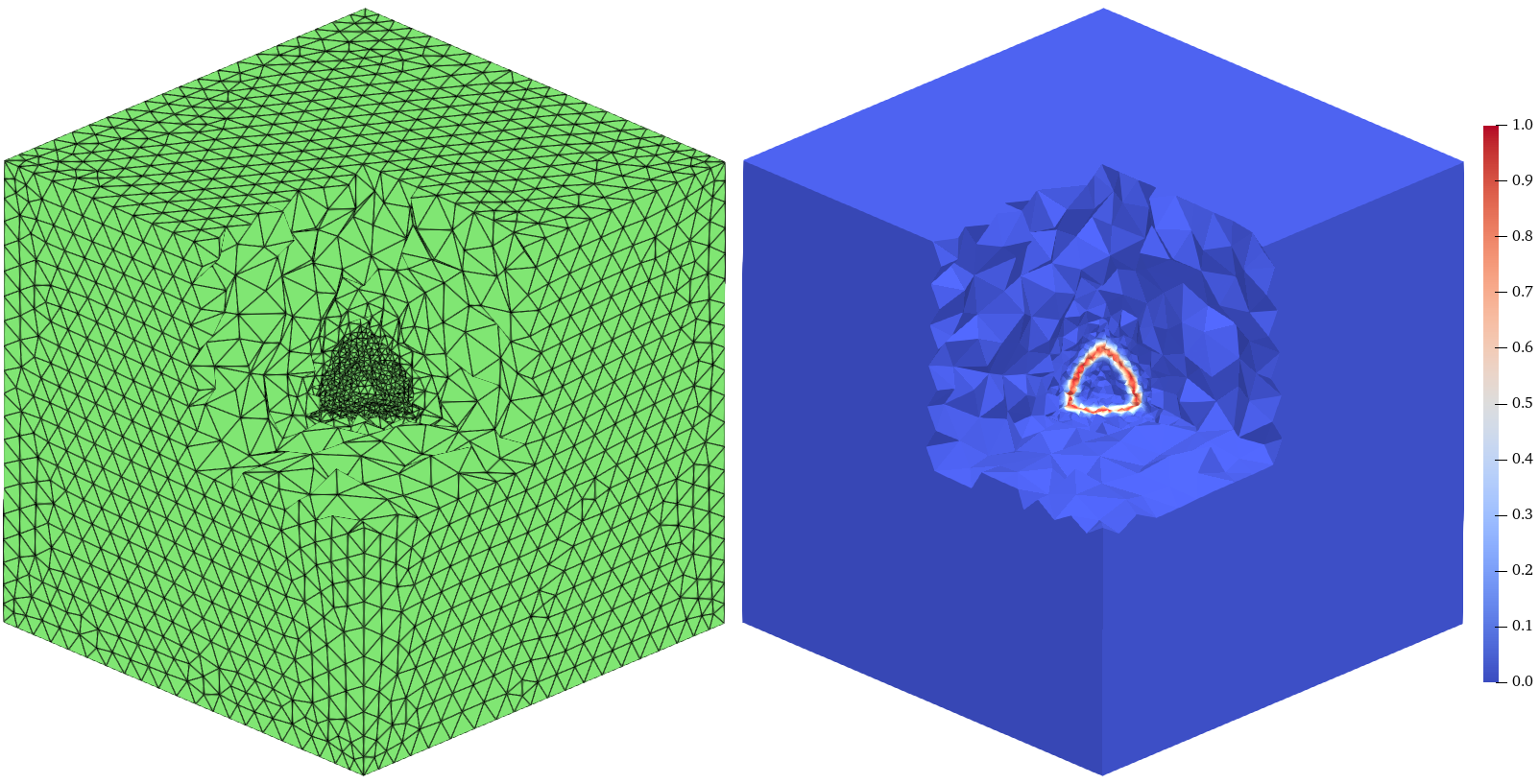
Figure 14. Example 4.5, snapshots of numerical solutions along with their corresponding adaptive meshes at 0.00, 0.25, 0.50, and 0.75 time.

Example 4.6.

(Splitting) Consider the 3D parabolic equation (1) in the domain $\Omega=[-1,1]^{3}$, with the source function $f$ such that the exact solution $u$ is given by:

$$u(x,y,z,t)=\exp(-300((x-0.3t)^{2}+y^{2}+z^{2}))+\exp(-300((x+0.3t)^{2}+y^{2}+z^{2})).$$

With the mesh refinement tolerance $eTol=0.1$, Figure 15 shows the adaptive process at $t=0$, terminating after seven steps and NOV at each iteration being 390, 615, 1062, 2085, 4606, 10860, and 27113, respectively. The mesh refinement process highlights that the adaptive algorithm achieves a highly efficient convergence procedure compared to traditional adaptive methods. Figure 16 illustrates the evolution of the numerical solutions and corresponding meshes at four distinct time points, capturing the symmetric splitting of the initial peak into two separate regions moving in opposite directions over time.

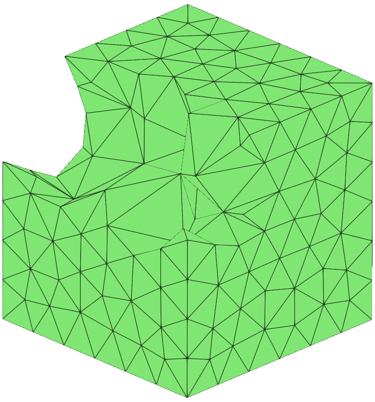
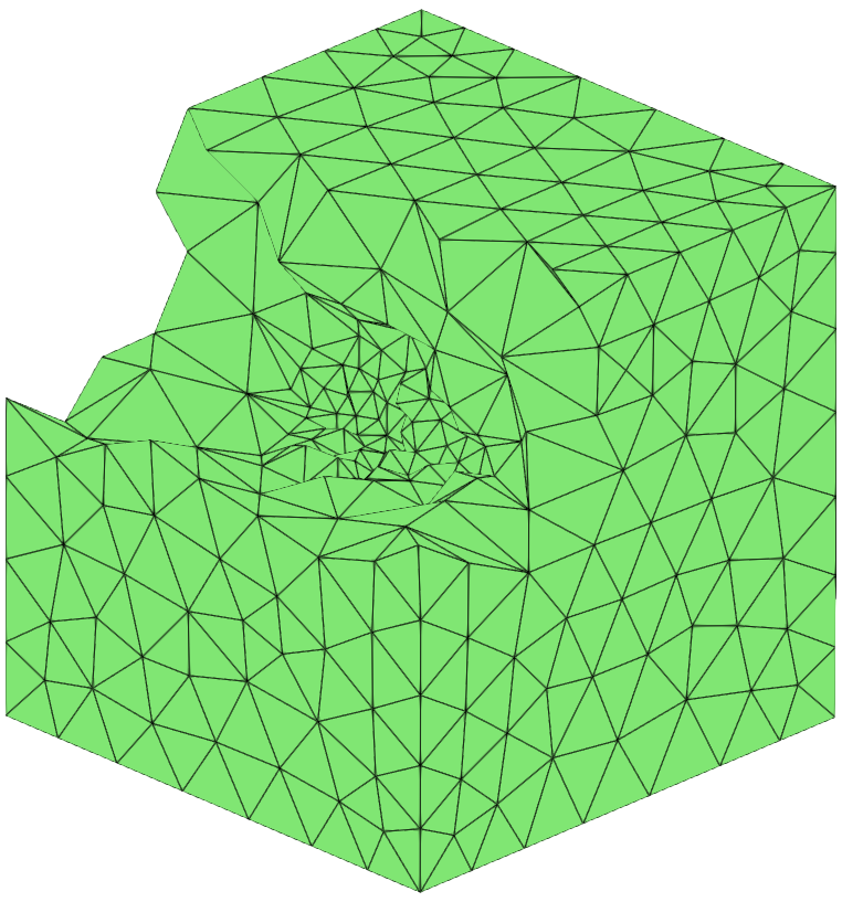
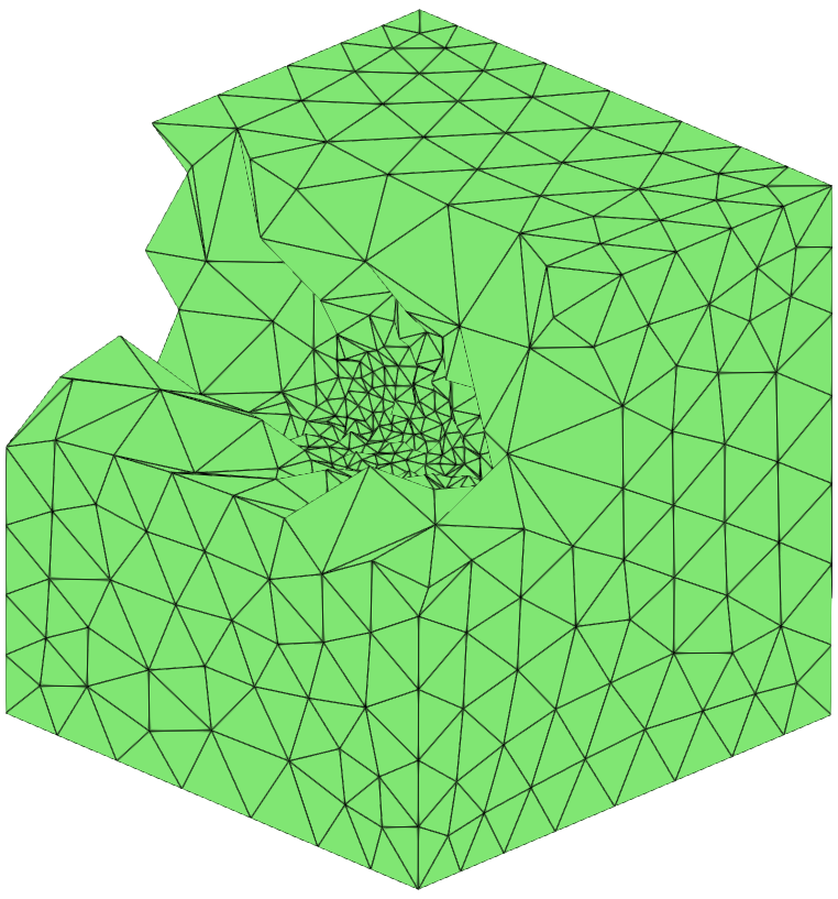
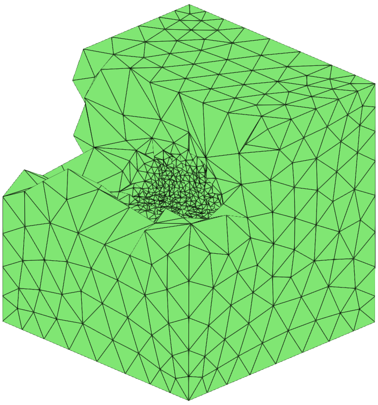
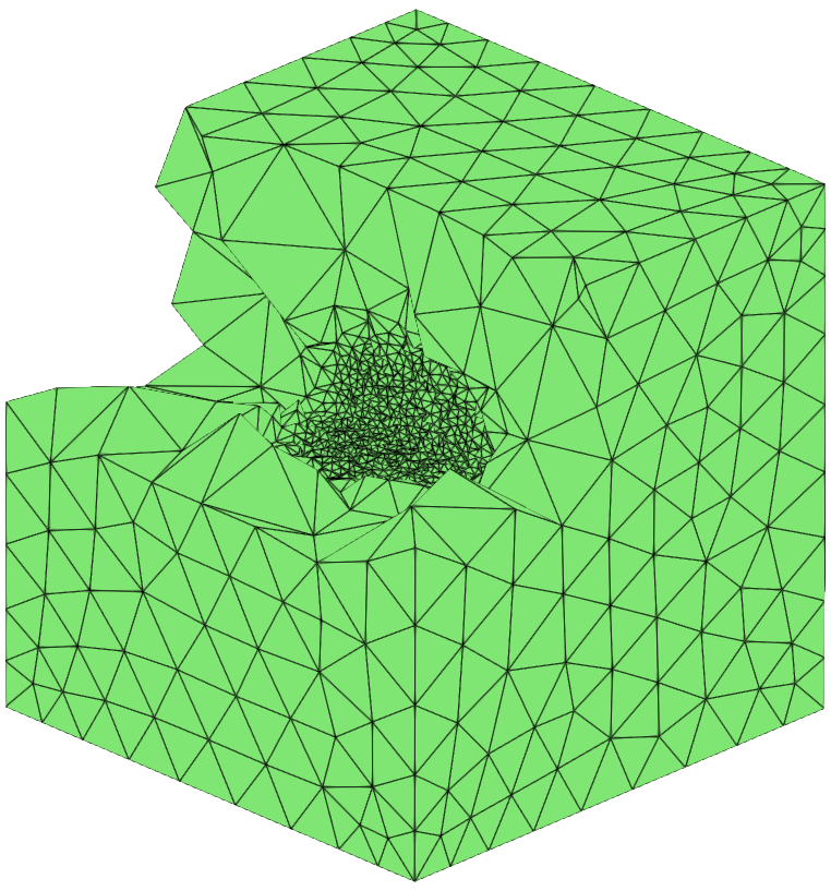
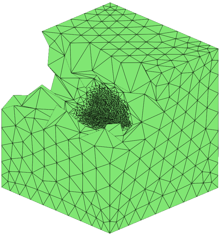
Figure 15. Example 4.6, initial mesh (left) and its evolution through five adaptive refinements at $t=0.0$.

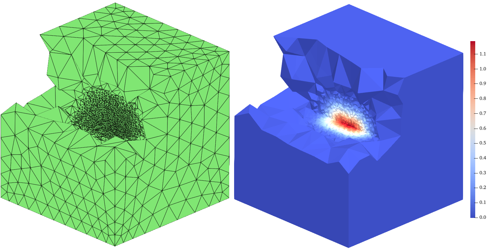
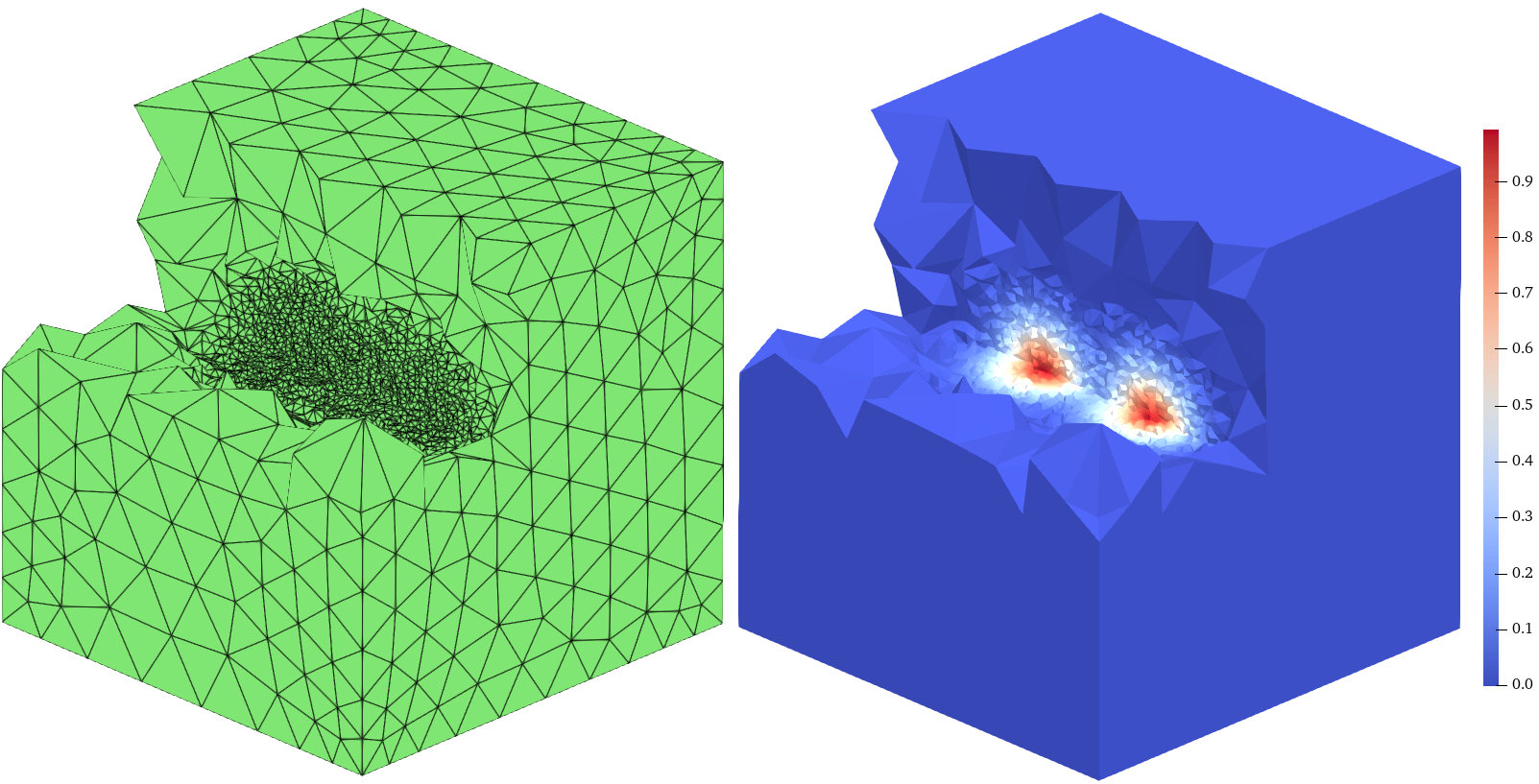
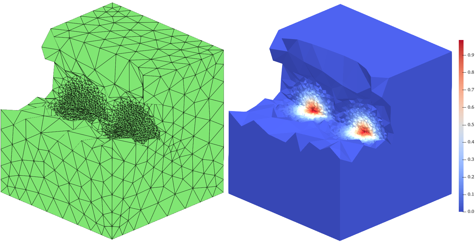
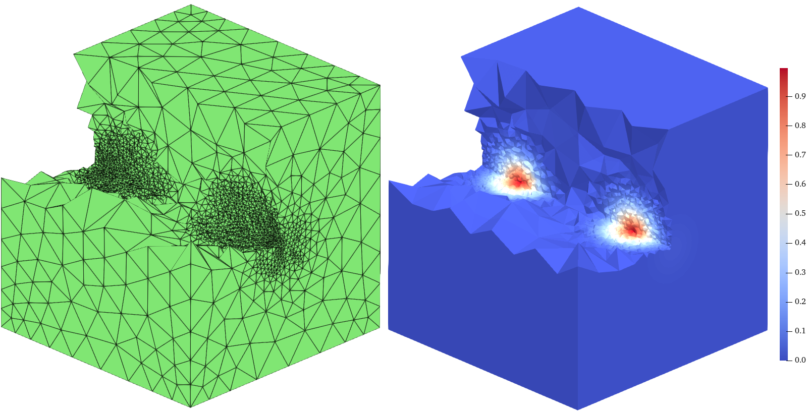
Figure 16. Example 4.6, snapshots of numerical solutions along with their corresponding adaptive meshes at 0.00, 0.25, 0.50, and 0.75 time.

References

- [1] R. Aboulaich, S. Boujena and E.E. Guarmah. A nonlinear parabolic model in processing of medical image. Mathematical Modelling of Natural Phenomena, 3(6):131-145, 2008.
- [2] M. Ainsworth and J.T. Oden. A posteriori error estimation in finite element analysis. Computer Methods in Applied Mechanics and Engineering, 142(1-2):1-88, 1997.
- [3] S.N. Antontsev, J.I. Diaz, S. Shmarev and A.J. Kassab. Energy methods for free boundary problems: Applications to nonlinear PDEs and fluid mechanics. Applied Mechanics Reviews, 55(4):B74-B75, 2002.
- [4] G. Barles, C. Daher and M. Romano. Convergence of numerical schemes for parabolic equations arising in finance theory. Mathematical Models and Methods in Applied Sciences, 5(1):125-143, 1995.
- [5] A.R. Barron. Universal approximation bounds for superpositions of a sigmoidal function. IEEE Transactions on Information Theory, 39(3):930-945, 1993.
- [6] A. Bonito, C. Canuto, R.H. Nochetto and A. Veeser. Adaptive finite element methods. Acta Numerica, 33:163-485, 2024.
- [7] Z. Cai, J. Chen and M. Liu. Self-adaptive deep neural network: Numerical approximation to functions and PDEs. Journal of Computational Physics, 455:111021, 2022.
- [8] J. Chen, X. Chi, W. E and Z. Yang. Bridging traditional and machine learning-based algorithms for solving PDEs: The random feature method. Journal of Machine Learning, 1(3):268-298, 2022.
- [9] Y. Chen, Y. Huang, N. Yi and P. Yin. Recovery Type a Posteriori Error Estimation of an Adaptive Finite Element Method for Cahn–Hilliard Equation. Journal of Scientific Computing, 98(2):35, 2024.
- [10] Z. Chen and J. Feng. An adaptive finite element algorithm with reliable and efficient error control for linear parabolic problems. Mathematics of Computation, 73(247):1167-1193, 2004.
- [11] W. E, C. Ma and L. Wu. The Barron space and the flow-induced function spaces for neural network models. Constructive Approximation, 55:369-406, 2021.
- [12] W. E and B. Yu. The deep Ritz method: A deep learning-based numerical algorithm for solving variational problems. Communications in Mathematics and Statistics, 6:1-12, 2018.
- [13] K. Eriksson and C. Johnson. Adaptive finite element methods for parabolic problems I: a linear model problem. SIAM Journal on Numerical Analysis, 28(1):43-77, 2006.
- [14] C. Geuzaine and J.-F. Remacle. Gmsh: A 3-D finite element mesh generator with built-in pre- and post-processing facilities. International Journal for Numerical Methods in Engineering, 79(11):1309-1331, 2009.
- [15] W. Gong, H. Liu and N. Yan. Adaptive finite element method for parabolic equations with dirac measure. Computer Methods in Applied Mechanics and Engineering, 328(1):217-241, 2018.
- [16] J. He, L. Li, J. Xu and C. Zheng. ReLU deep neural networks and linear finite elements. Journal of Computational Mathematics, 38(3):502-527, 2020.
- [17] K. He, X. Zhang, S. Ren and J. Sun. Deep residual learning for image recognition. 2016 IEEE Conference on Computer Vision and Pattern Recognition, 770-778, 2016.
- [18] K. Hornik. Approximation capabilities of multilayer feedforward networks. Neural Networks, 4(2):251-257, 1991.
- [19] K. Hornik, M. Stinchcombe and H. White. Multilayer feedforward networks are universal approximators. Neural Networks, 2(5):359-366, 1989.
- [20] Y. Huang, K. Jiang and N. Yi. Some weighted averaging methods for gradient recovery. Advances in Applied Mathematics and Mechanics, 4(2):131-155, 2012.
- [21] Y. Huang and N. Yi. The superconvergent cluster recovery method. Journal of Scientific Computing, 44(3):301-322, 2010.
- [22] D. Khurana, A. Koli, K. Khatter and S. Singh. Natural language processing: state of the art, current trends and challenges. Multimedia Tools and Applications, 82(3):3713–3744, 2023.
- [23] I.E. Lagaris, A. Likas and D.I. Fotiadis. Artificial neural networks for solving ordinary and partial differential equations. IEEE Transactions on Neural Networks, 9(5):987-1000, 1998.
- [24] O. Lakkis and T. Pryer. Gradient recovery in adaptive finite-element methods for parabolic problems. IMA Journal of Numerical Analysis, 32(1):246-278, 2012.
- [25] Y. Liu, J. Xiao, N. Yi and H. Cao. Gradient recovery-based a posteriori error estimator and adaptive finite element method for elliptic equations. submited, 2024.
- [26] K. Mekchay and R.H. Nochetto. Convergence of adaptive finite element methods for general second order linear elliptic PDEs. SIAM Journal on Numerical Analysis, 43(5):1803–1827, 2005.
- [27] P. Morin, R.H. Nochetto and K.G. Siebert. Convergence of adaptive finite element methods. SIAM Review, 44(4):631–658, 2002.
- [28] N. Sukumar and A. Srivastava. Exact imposition of boundary conditions with distance functions in physics-informed deep neural networks. Computer Methods in Applied Mechanics and Engineering, 389:114333, 2022.
- [29] M. Picasso. Adaptive finite elements for a linear parabolic problem. Computer Methods in Applied Mechanics and Engineering, 167(3-4):223-237, 1998.
- [30] M. Raissi, P. Perdikaris and G.E. Karniadakis. Physics-informed neural networks: A deep learning framework for solving forward and inverse problems involving nonlinear partial differential equations. Journal of Computational Physics, 378(1):686-707, 2019.
- [31] P. Rogolino, R. Kovács, P. Ván and V.A. Cimmelli. Generalized heat-transport equations: parabolic and hyperbolic models. Continuum Mechanics and Thermodynamics, 30(6):1245–1258, 2018.
- [32] J.W. Siegel and J. Xu. Approximation rates for neural networks with general activation functions. Neural Networks, 128:313-321, 2020.
- [33] R. Verfürth. A posteriori error estimation techniques for finite element methods. Oxford University Press, 2013.
- [34] X. Wang, X. Duan and Y. Gao. Multiscale asymptotic analysis and parallel algorithm of parabolic equation in composite materials. Mathematical Problems in Engineering, 2014(3):1-12, 2014.
- [35] O. Wilderotter. An adaptive finite element method for singular parabolic equations. Numerische Mathematik, 96(2):377-399, 2003.
- [36] J. Xiao, Y. Liu and N. Yi. High accuracy techniques based adaptive finite element methods for elliptic PDEs. submited, 2025.
- [37] J. Xu. Finite neuron method and convergence analysis. Communications in Computational Physics, 28(5):1707-1745, 2020.
- [38] D. Yarotsky. Error bounds for approximations with deep ReLU networks. Neural Networks, 94:103–114, 2017.
- [39] S. Zeng, Z. Zhang and Q. Zou. Adaptive deep neural networks methods for high-dimensional partial differential equations. Journal of Computational Physics, 463:111232, 2022.
- [40] Z. Zhang and A. Naga. A new finite element gradient recovery method: Superconvergence property. SIAM Journal on Scientific Computing, 26(4):1192-1213, 2005.
- [41] O.C. Zienkiewicz and J. Zhu. The superconvergent patch recovery and a posteriori error estimates. Part 1: The recovery technique. International Journal for Numerical Methods in Engineering, 33(7):1331-1364, 1992.