Exploiting Multistage Optimization Structure in Proximal Solvers

Abstract

This paper presents an efficient structure-exploiting algorithm for multistage optimization problems, implemented as a new backend in the PIQP solver. The proposed method extends existing approaches by supporting full coupling between stages and global decision variables in the cost as well as equality and inequality constraints. The solver leverages a specialized block-tri-diagonal-arrow Cholesky factorization within a proximal interior-point framework to handle the underlying problem structure efficiently. The implementation features automatic structure detection and seamless integration with existing interfaces. Numerical experiments demonstrate significant performance improvements, achieving up to 13x speed-up compared to a generic sparse backend and matching/exceeding the performance of the state-of-the-art specialized solver HPIPM. The solver is particularly effective for applications such as model predictive control, robust scenario optimization, and periodic optimization problems.

I Introduction

The efficient solution of convex optimization problems is crucial across engineering disciplines, particularly in real-time applications. An important category is the class of multistage optimization problems, which arise naturally in various domains, including model predictive control (MPC) and multistage portfolio optimization. These problems are characterized by a sequence of interconnected stages, often coupled through both the constraints and the cost function.

While numerous solvers have been developed for multistage optimization problems, most impose restrictive assumptions on the underlying problem structure. A comprehensive list of multistage quadratic programming (QP) solvers can be found in Table I. These solvers typically support coupling between consecutive stages only through equality constraints or forward system dynamics, limiting their applicability to more general problems. This limitation extends to non-linear optimization solvers like FATROP [1] or FORCES NLP [2]. Though [3] and [4] consider global decision variables, they assume independent stages without coupling. Many problems, including periodic optimization [5], robust scenario MPC [6], or tracking MPC [7], can be naturally formulated as multistage optimization problems with global decision variables.

This paper extends these approaches to solving general multistage optimization problems. We support both full coupling between stages and global decision variables in the cost and all constraint types. The main contributions are: (1) the exploitation of the block-tri-diagonal-arrow structure of the KKT matrix that naturally arises from this coupling and (2) the automatic detection of this structure from standard sparse problem formulations. Although we present our method within a proximal interior-point framework, the structure-exploiting factorization can be easily integrated into various proximal-based solvers like OSQP [8]. Additionally, we provide seamless integration with existing interfaces through automatic structure detection that is invariant to constraint ordering, significantly reducing implementation burden.

The proposed method is implemented as a new backend in the PIQP solver [9], combining the robustness of proximal interior-point methods with the efficiency of structure-exploiting linear algebra. Our numerical experiments demonstrate significant performance improvements, achieving up to 13x speed-up compared to the generic sparse backend. Notably, the solver maintains or exceeds the performance of state-of-the-art solvers like HPIPM [10].

Section II presents the problem formulation. Section III reviews the proximal interior-point method underlying our approach. Section IV introduces our structure-exploiting factorization routines, followed by implementation details in Section V. Finally, numerical results are presented in Section VI, showcasing the solver’s performance.

Notation

We denote the set of $n$-dimensional real vectors by $\mathbb{R}^{n}$, and the set of $n\times m$-dimensional real matrices by $\mathbb{R}^{n\times m}$. Moreover, the subspace of symmetric matrices in $\mathbb{R}^{n\times n}$ is denoted by $\mathbb{S}^{n}$, and the cone of positive semi-definite matrices in $\mathbb{S}^{n}$ by $\mathbb{S}_{+}^{n}$. The identity matrix is denoted by $I_{n}\in\mathbb{R}^{n\times n}$ and a vector filled with ones by $\mathbf{1}_{n}\in\mathbb{R}^{n}$.

II Problem Formulation

We consider the multistage optimization problem

$$\min_{x,g} \sum_{i=0}^{N-1}\ell_{i}(x_{i},x_{i+1},g)+\ell_{N}(x_{N},g)$$ (1)

s.t. $$A_{i}x_{i}+B_{i}x_{i+1}+E_{i}g=b_{i},\hskip 5.0pti=0,\dots,N-1,$$

$$C_{i}x_{i}+D_{i}x_{i+1}+F_{i}g\leq h_{i},\hskip 3.99994pti=0,\dots,N-1,$$

$$A_{N}x_{N}+E_{N}g=b_{N},$$

$$D_{N}x_{N}+F_{N}g\leq h_{N},$$

with $N$ stages and coupled stage cost

TABLE I: Comparison of Structure-Exploiting Multistage QP Solvers

Characteristics	PIQP	Forces [11]	HPIPM [10]	QPALM-OCP [12]	ASIPM [13]
Algorithm	PALM-IP	IP	IP	PALM	Inexact IP
Stage-wise Structure	Yes	Yes	Yes	Yes	Yes
Global Variables	Yes	No	No	No	No
Inter-stage Coupling	Full	Equality only	Forward dynamics	Forward dynamics	Forward dynamics
Implementation	C++	C	C	Matlab/Codegen	C
License Type	BSD-2	Commercial	BSD-2	Closed	Closed

$$\ell_{i}(x_{i},x_{i+1},g)\!\coloneqq\!\frac{1}{2}\!\begin{bmatrix}x_{i}\\ x_{i+1}\\ g\end{bmatrix}^{\top}\!\!\begin{bmatrix}Q_{i}&S_{i}^{\top}&T_{i}^{\top}\\ S_{i}&0&0\\ T_{i}&0&0\end{bmatrix}\!\!\!\begin{bmatrix}x_{i}\\ x_{i+1}\\ g\end{bmatrix}\!+c_{i}^{\top}x_{i},$$

and terminal cost

$$\ell_{N}(x_{N},g)\coloneqq\frac{1}{2}\begin{bmatrix}x_{N}\\ g\end{bmatrix}^{\top}\begin{bmatrix}Q_{N}&T_{N}^{\top}\\ T_{N}&Q_{g}\end{bmatrix}\begin{bmatrix}x_{N}\\ g\end{bmatrix}+c_{N}^{\top}x_{N}+c_{g}^{\top}g,$$

where $x_{i}\in\mathbb{R}^{n_{i}}$ are the stage-wise decision variables, $g\in\mathbb{R}^{n_{g}}$ is a global decision variable, and $N\in\mathbb{N}$ is the horizon. The matrices $Q_{i}\in\mathbb{S}_{+}^{n_{i}}$, $S_{i}\in\mathbb{R}_{+}^{n_{i+1}\times n_{i}}$, and $T_{i}\in\mathbb{R}_{+}^{n_{g}\times n_{i}}$ together with $c_{i}\in\mathbb{R}^{n_{i}}$ and $c_{g}\in\mathbb{R}^{n_{g}}$ encode the coupled cost. The stage-wise variables are also coupled through equality and inequality constraints encoded by $A_{i}\in\mathbb{R}^{p_{i}\times n_{i}}$, $B_{i}\in\mathbb{R}^{p_{i}\times n_{i+1}}$, $E_{i}\in\mathbb{R}^{p_{i}\times n_{g}}$, $b_{i}\in\mathbb{R}^{p}$, $C_{i}\in\mathbb{R}^{m_{i}\times n_{i}}$, $D_{i}\in\mathbb{R}^{m_{i}\times n_{i+1}}$, and $h_{i}\in\mathbb{R}^{m_{i}\times n_{g}}$, respectively. Note that the formulation (1) is more general than the typical optimal control problem (OCP) formulations in the literature, as the stages are not only coupled through the system dynamics.

We can reformulate problem (1) into a general QP form

$$\min_{x,s} \frac{1}{2}x^{\top}Px+c^{\top}x$$ (2)

s.t. $$Ax=b,$$

$$Gx-h+s=0,$$

$$s\geq 0,$$

where the stages $x_{i}$ and the global variable $g$ are collected into the decision variable $x=(x_{0},\dots,x_{N},g)\in\mathbb{R}^{n}$ with $n=\sum_{i=0}^{N}n_{x_{i}}+n_{g}$. The cost is now defined by a block-tri-diagonal-arrow matrix $P\in\mathbb{R}^{n\times n}$ and $c\in\mathbb{R}^{n}$. By introducing the slack variable $s\in\mathbb{R}^{m}$ with $m=\sum_{i=0}^{N}m_{i}$, we lift the affine inequality constraints to equality constraints, leaving us with a simple non-negativity constraint and the equality constraints defined by $A\in\mathbb{R}^{p\times n}$, $b\in\mathbb{R}^{p}$, $G\in\mathbb{R}^{m\times n}$, and $h\in\mathbb{R}^{m}$, with $p=\sum_{i=0}^{N}p_{i}$.

III Proximal Interior-Point

This section introduces the interior-point method developed in [9]. While the factorization algorithms presented in this paper should generalize to most proximal-based solvers, we demonstrate the effectiveness of the proposed method using the algorithm in PIQP.

The proximal augmented Lagrangian of problem (2) is given as

$$\mathcal{L}_{\rho,\delta}(x,s ;\xi,\lambda,\nu)\coloneqq\frac{1}{2}x^{\top}Px+c^{\top}x+\frac{\rho}{2}\left\|x-\xi\right\|_{2}^{2}$$ (3)

$$+\lambda^{\top}(Ax-b)+\frac{1}{2\delta}\|Ax-b\|_{2}^{2}$$

$$+\nu^{\top}(Gx-h+s)+\frac{1}{2\delta}\|Gx-h+s\|_{2}^{2},$$

where the variables $\lambda\in\mathbb{R}^{p}$ and $\nu\in\mathbb{R}^{m}$ are the Lagrange multipliers of the equality constraints in (2), $\xi\in\mathbb{R}^{n}$ acts as a regularizer, and $\rho,\delta>0$ are penalty parameters. The proximal method of multipliers, proposed in [14], is then given by

$$(\xi^{k+1},s^{k+1}) \in\underset{x,s\geq 0}{\text{argmin}}\;\mathcal{L}_{\rho_{k},\delta_{k}}(x,s;\xi^{k},\lambda^{k},\nu^{k}),$$ (4a)

$$\lambda^{k+1} =\lambda^{k}+\frac{1}{\delta_{k}}\left(A\xi^{k+1}-b\right),$$ (4b)

$$\nu^{k+1} =\nu^{k}+\frac{1}{\delta_{k}}\left(G\xi^{k+1}-h+s^{k+1}\right),$$ (4c)

where $\xi$ is used to represent the $x$ variable in the proximal method of multipliers.

PIQP follows the method proposed in [15], where one iteration of the interior-point method is applied to (4a). More specifically, we replace the inequality constraint in (4a) with the log-barrier $\Phi_{\mu}(s)=-\mu\sum_{i=1}^{m}\ln[s]_{i}$ resulting in the minimization problem

$$\underset{x,s}{\text{min}}\;\mathcal{L}_{\rho_{k},\delta_{k}}(x,s;\xi^{k},\lambda^{k},\nu^{k})+\sigma_{k}\cdot\Phi_{\mu_{k}}(s),$$ (5)

where $[s]_{i}$ denotes the $i$-th element of $s$, $\mu>0$ is the barrier parameter, and $\sigma_{k}\in(0,1]$ is a scaling parameter. The resulting first-order optimality conditions of (5) are then given by

$$Px+c+\rho_{k}(x-\xi^{k})+A^{\top}y+G^{\top}z =0,$$ (6a)

$$Ax-\delta_{k}(y-\lambda^{k})-b =0,$$ (6b)

$$Gx-\delta_{k}(z-\nu^{k})-h+s =0,$$ (6c)

$$s\circ z-\sigma_{k}\mu_{k}\mathbf{1}_{m} =0,$$ (6d)

with auxiliary variables $y\coloneqq\lambda^{k}+\frac{1}{\delta_{k}}(Ax-b)$ and $z\coloneqq\nu^{k}+\frac{1}{\delta_{k}}(Gx-h+s)$, simplifying the equations and the updates (4b) and (4c). Here, the $\circ$ operator indicates elementwise multiplication. Solving (6) using Newton’s method amounts to solving the following linear equation at iteration $k$

$$\begin{bmatrix}P+\rho_{k}I_{n}&A^{\top}&G^{\top}&0\\ A&-\delta_{k}I_{p}&0&0\\ G&0&-\delta_{k}I_{m}&I_{m}\\ 0&0&S^{k}&Z^{k}\end{bmatrix}\begin{bmatrix}\Delta x^{k}\\ \Delta y^{k}\\ \Delta z^{k}\\ \Delta s^{k}\end{bmatrix}=\begin{bmatrix}r^{k}_{x}\\ r^{k}_{y}\\ r^{k}_{z}\\ r^{k}_{s}\end{bmatrix}$$ (7)

with initialization $(x^{k},y^{k},z^{k},s^{k})$, $S^{k},Z^{k}\in\mathbb{R}^{m\times m}$ are diagonal matrices with $s^{k}$, $z^{k}$ on its diagonal, and residuals

$$r^{k}_{x} =-(Px^{k}+c+\rho_{k}(x^{k}-\xi^{k})+A^{\top}y^{k}+G^{\top}z^{k}),$$

$$r^{k}_{y} =-(Ax^{k}+\delta_{k}(\lambda^{k}-y^{k})-b),$$

$$r^{k}_{z} =-(Gx^{k}+\delta_{k}(\nu^{k}-z^{k})-h+s^{k}),$$

$$r^{k}_{s} =-s^{k}\circ z^{k}+\sigma_{k}\mu_{k}\mathbf{1}_{m}.$$

Eliminating $\Delta s^{k}$ in (7) results in a reduced system of equations

$$\underbrace{\begin{bmatrix}P+\rho^{k}I_{n}&\!\!\!A^{\top}&\!\!\!G^{\top}\\ A&\!\!\!-\delta^{k}I_{p}&\!\!\!0\\ G&\!\!\!0&\!\!\!-(W^{k}+\delta^{k}I_{m})\end{bmatrix}}_{J(s^{k},z^{k})}\begin{bmatrix}\Delta x^{k}\\ \Delta y^{k}\\ \Delta z^{k}\end{bmatrix}=\begin{bmatrix}r^{k}_{x}\\ r^{k}_{y}\\ \bar{r}^{k}_{z}\end{bmatrix}$$

with the Nesterov-Todd scaling $W^{k}=(Z^{k})^{-1}S^{k}$ and $\bar{r}^{k}_{z}=r^{k}_{z}-(Z^{k})^{-1}r^{s}_{k}$ [16]. The slack direction $\Delta s^{k}$ can then be reconstructed with $\Delta s^{k}=(Z^{k})^{-1}(r^{k}_{s}-S^{k}\Delta z^{k})$.

In the remainder of the paper, we will focus on how to solve $J(s^{k},z^{k})$ as efficiently as possible, exploiting the underlying structure. Thus, we will not go into further details concerning the interior-point method itself. The interested reader is referred to [9] for more details.

Note that the structure of $J(s^{k},z^{k})$ is ubiquitous and is present in almost all proximal-based solvers. For example, OSQP [8] has the exact same KKT structure. Hence, the factorization scheme presented in the next section is directly transferable.

IV Solution of the Linearized KKT System

The symmetry of $J(s^{k},z^{k})$ enables the use of a sparse LDL factorization, as the regularization terms ensure the matrix is quasi-definite [17]. While this approach was adopted in the original PIQP solver due to its general treatment of $P$, $A$, and $G$ without exploiting their structure, the multistage nature of our problem presents an opportunity for more efficient computation.

Eliminating $\Delta z^{k}$ gives the so-called augmented system

$$\begin{bmatrix}\Phi&\!\!\!A^{\top}\\ A&\!\!\!-\delta^{k}I_{p}\end{bmatrix}\begin{bmatrix}\Delta x^{k}\\ \Delta y^{k}\end{bmatrix}=\begin{bmatrix}\bar{r}^{k}_{x}\\ r^{k}_{y}\end{bmatrix}$$

where

$$\Phi =P+\rho^{k}I_{n}+G^{\top}(W^{k}+\delta_{k}I_{m})^{-1}G,$$ (8)

$$\bar{r}^{k}_{x} =r^{k}_{x}+G^{\top}(W^{k}+\delta_{k}I)^{-1}\bar{r}^{k}_{z},$$

$$\Delta z^{k} =(W^{k}+\delta_{k}I)^{-1}(G\Delta x^{k}-\bar{r}^{k}_{z}).$$

The usual approach in the interior-point literature would be to eliminate $\Delta x^{k}$ to obtain the so-called normal equations since there is usually no regularization from the proximal terms, i.e. $\delta^{k}=0$ [11, 12]. However, this destroys the sparsity pattern assuming our more general structure, that is, $\Phi^{-1}$ is dense due to the coupling between stages in the cost and inequalities. Instead, we eliminate $\Delta y^{k}$, yielding the system

$$\Psi\Delta x^{k}=\bar{r}^{k}$$ (9)

where

$$\Psi =(\Phi+\delta_{k}^{-1}A^{\top}A),$$ (10)

$$\bar{r}^{k} =\bar{r}^{k}_{x}+\delta_{k}^{-1}A^{\top}r^{k}_{y},$$

$$\Delta y^{k} =\delta_{k}^{-1}(A\Delta x_{k}-r^{k}_{y}).$$

While this approach shares similarities with [13] and [4], it differs fundamentally in its treatment of regularization terms. These works introduce the regularization terms heuristically, compromising either convergence guarantees or computational efficiency through required post-processing steps such as iterative refinement.

IV-A Block-tri-diagonal-arrow Cholesky Factorization

The symmetric matrix $\Psi$ is positive-definite and has the block-tri-diagonal-arrow structure

$$\Psi\!\coloneqq\!\begin{bmatrix}\Psi_{0,0}&\!\!\!\Psi_{1,0}^{\top}&\!\!\!0&\!\!\!\cdots&\!\!\!\Psi_{N+1,0}^{\top}\\[4.30554pt] \Psi_{1,0}&\!\!\!\Psi_{1,1}&\!\!\!\Psi_{1,2}^{\top}&\!\!\!\ddots&\!\!\!\Psi_{N+1,1}^{\top}\\ 0&\!\!\!\Psi_{1,2}&\!\!\!\ddots&\!\!\!\ddots&\!\!\!\vdots\\ \vdots&\!\!\!\ddots&\!\!\!\ddots&\!\!\!\Psi_{N,N}&\!\!\!\Psi_{N+1,N}^{\top}\\[4.30554pt] \Psi_{N+1,0}&\!\!\!\Psi_{N+1,1}&\!\!\!\cdots&\!\!\!\Psi_{N+1,N}&\!\!\!\Psi_{N+1,N+1}\end{bmatrix}$$

Algorithm 1 Construction of $\Psi$

1:$\Psi_{0,0}\leftarrow Q_{0}+\rho_{k}I_{n_{0}}+\delta_{k}^{-1}A_{0}^{\top}A_{0}+C_{0}^{\top}(W^{k}_{0}+\delta_{k})^{-1}C_{0}$

2:$\Psi_{N+1,0}\leftarrow T_{0}+\delta^{-1}_{k}E_{0}^{\top}A_{0}+F_{0}^{\top}(W^{k}_{0}+\delta_{k})^{-1}C_{0}$

3:for $i=0,\ldots,N-1$ do

4:  $\Psi_{i+1,i+1}\leftarrow Q_{i+1}+\rho_{k}I_{n_{i+1}}$

5:$\hskip 90.70021pt+\delta_{k}^{-1}A_{i+1}^{\top}A_{i+1}+\delta_{k}^{-1}B_{i}^{\top}B_{i}$

6:$\hskip 90.70021pt+C_{i+1}^{\top}(W^{k}_{i+1}+\delta_{k})^{-1}C_{i+1}$

7:$\hskip 90.70021pt+D_{i}^{\top}(W^{k}_{i}+\delta_{k})^{-1}D_{i}$

8:  $\Psi_{i+1,i}\leftarrow S_{i}+\delta_{k}^{-1}B_{i}^{\top}A_{i}+D_{i}^{\top}(W^{k}_{i}+\delta_{k})^{-1}C_{i}$

9:  $\Psi_{N+1,i+1}\leftarrow T_{i+1}+\delta_{k}^{-1}E_{i+1}^{\top}A_{i+1}+\delta_{k}^{-1}E_{i}^{\top}B_{i}$

10:$\hskip 92.90007pt+F_{i+1}^{\top}(W^{k}_{i+1}+\delta_{k})^{-1}C_{i+1}$

11:$\hskip 92.90007pt+F_{i}^{\top}(W^{k}_{i}+\delta_{k})^{-1}D_{i}$

12:end for

13:$\Psi_{N+1,N+1}\leftarrow Q_{g}+\rho_{k}I_{n_{g}}+\sum_{j=0}^{N}\delta_{k}^{-1}E_{j}^{\top}E_{j}$

14:$\hskip 75.50014pt+\sum_{j=0}^{N}F_{j}^{\top}(W^{k}_{j}+\delta_{k})^{-1}F_{j}$

The constructions of $\Psi$ and $\bar{r}^{k}$ are described in Algorithm 1 and Algorithm 2, respetively.

Algorithm 2 Construction of $\bar{r}^{k}$

1:$\bar{r}^{k}_{0}\leftarrow r^{k}_{x,0}+\delta_{k}^{-1}A_{0}^{\top}r^{k}_{y,0}+C_{0}^{\top}(W_{0}^{k}+\delta_{k}I)^{-1}\bar{r}^{k}_{z,0}$

2:for $i=1,\ldots,N$ do

3:  $\bar{r}^{k}_{i}\leftarrow r^{k}_{x,i}+\delta_{k}^{-1}A_{i}^{\top}r^{k}_{y,i}+\delta_{k}^{-1}B_{i-1}^{\top}r^{k}_{y,i-1}$

4:$\hskip 57.40013pt+C_{i}^{\top}(W_{i}^{k}+\delta_{k}I)^{-1}\bar{r}^{k}_{z,i}$

5:$\hskip 57.40013pt+D_{i-1}^{\top}(W_{i-1}^{k}+\delta_{k}I)^{-1}\bar{r}^{k}_{z,i-1}$

6:end for

7:$\bar{r}^{k}_{N+1}\leftarrow\sum_{i=0}^{N}\left(\delta_{k}^{-1}E_{i}^{\top}r^{k}_{y,i}+F_{i}^{\top}(W_{i}^{k}+\delta_{k}I)^{-1}\bar{r}^{k}_{z,i}\right)$

The Cholesky factorization $LL^{\top}=\Psi$ preserves the block-tri-diagonal-arrow structure of $\Psi$, with the lower triangular factor $L$ taking the form

$$L\!:=\!\begin{bmatrix}L_{0,0}&\!\!\!0&\!\!\!0&\!\!\!\cdots&\!\!\!0\\ L_{1,0}&\!\!\!L_{1,1}&\!\!\!0&\!\!\!\ddots&\!\!\!0\\ 0&\!\!\!L_{1,2}&\!\!\!\ddots&\!\!\!\ddots&\!\!\!\vdots\\ \vdots&\!\!\!\ddots&\!\!\!\ddots&\!\!\!L_{N,N}&\!\!\!0\\[4.30554pt] L_{N+1,0}&\!\!\!L_{N+1,1}&\!\!\!\cdots&\!\!\!L_{N+1,N}&\!\!\!L_{N+1,N+1}\end{bmatrix}$$ (11)

The computation of $L$ follows the procedure detailed in Algorithm 3.

Algorithm 3 Factorization of $\Psi$

1:$L_{0,0}\leftarrow\operatorname{chol}\left(\Psi_{0,0}\right)$

2:$L_{N+1,0}\leftarrow\Psi_{N+1,0}L_{0,0}^{-\top}$

3:for $i=1,\ldots,N$ do

4:  $L_{i,i}\leftarrow\operatorname{chol}\left(\Psi_{i,i}-L_{i,i-1}L_{i,i-1}^{\top}\right)$

5:  $L_{i,i-1}\leftarrow\Psi_{i,i-1}L_{i-1,i-1}^{-\top}$

6:  $L_{N+1,i}\leftarrow\left(\Psi_{N+1,i}-L_{N+1,i-1}L_{i,i-1}^{\top}\right)L_{i,i}^{-\top}$

7:end for

8:$L_{N+1,N+1}\!\leftarrow\!\operatorname{chol}\left(\Psi_{N+1,N+1}\!-\!\sum_{i=0}^{N}L_{N+1,i}L_{N+1,i}^{\top}\right)$

$\Delta x^{k}$ is computed through standard forward and backward substitution steps, as described in Algorithm 4.

While the literature extensively documents Cholesky factorizations for both block-arrow and block-tri-diagonal matrices, the factorization of matrices with a combined block-tri-diagonal-arrow structure appears to be unexplored. This paper presents, to the best of our knowledge, the first comprehensive treatment of this specialized factorization pattern.

Algorithm 4 Solving for $\Delta x^{k}$

1:Forward Substitution

2:$\Delta x^{k}_{0}\leftarrow L_{0,0}^{-1}\bar{r}^{k}_{0}$

3:for $i=1,\ldots,N$ do

4:  $\Delta x^{k}_{i}\leftarrow L_{i,i}^{-1}\left(\bar{r}^{k}_{i}-L_{i,i-1}\Delta x^{k}_{i-1}\right)$

5:end for

6:$\Delta x^{k}_{N+1}\leftarrow L_{N+1,N+1}^{-1}\left(\bar{r}^{k}_{N+1}-\sum_{j=0}^{N}L_{N+1,j}\Delta x^{k}_{j}\right)$

7:Backward Substitution

8:$\Delta x^{k}_{N+1}\leftarrow L_{N+1,N+1}^{-\top}\Delta x^{k}_{N+1}$

9:$\Delta x^{k}_{N}\leftarrow L_{N,N}^{-\top}\left(\Delta x^{k}_{N}-L_{N+1,N}\Delta x^{k}_{N+1}\right)$

10:for $i=N-1,\ldots,0$ do

11:  $\Delta x^{k}_{i}\leftarrow L_{i,i}^{-1}\left(\Delta x^{k}_{i}\!-\!L_{i+1,i}\Delta x^{k}_{i+1}\!-\!L_{N+1,i}\Delta x^{k}_{N+1}\right)$

12:end for

IV-B Flop Analysis

To analyze the computational complexity, we evaluate the floating point operations (flops) required by our method. To be able to compare with existing literature, we base our analysis on a variant of the extended linear quadratic control problem inspired by [18]

$$\min_{z,u,g} \sum_{i=0}^{N-1}\ell_{i}(z_{i},u_{i},g)+\ell_{N}(z_{i},g)$$ (12)

s.t. $$z_{i+1}=\mathcal{A}_{i}z_{i}+\mathcal{B}_{i}u_{i}+E_{i}g+b_{i},$$

with state $z_{i}\in\mathbb{R}^{n_{x}}$, inputs $u_{i}\in\mathbb{R}^{n_{u}}$, and system dynamics $\mathcal{A}_{i}\in\mathbb{R}^{n_{x}\times n_{x}}$, $\mathcal{B}_{i}\in\mathbb{R}^{n_{x}\times n_{u}}$. For our formulation (1), we define $x_{i}=(z_{i},u_{i})$, $A_{i}=\begin{bmatrix}\mathcal{A}_{i}&\mathcal{B}_{i}\end{bmatrix}$, $B_{i}=\begin{bmatrix}-I_{n_{x}}&0_{n_{x}\times n_{u}}\end{bmatrix}$, and $S_{i}=0$ for $i=0,\dots,N-1$. Note, the structure of $B_{i}$, specifically its zero block, reduces the dimensions of the coupling matrices to $\Psi_{i+1,i},L_{i+1,i}\in\mathbb{R}^{n_{x}\times(n_{x}+n_{u})}$ rather than $\mathbb{R}^{(n_{x}+n_{u})\times(n_{x}+n_{u})}$.

Using the elementary matrix operation costs from Table II, we derive the computational complexity of both factorization and solution steps, presented in Table III. For $n_{g}=0$, our results align with previous findings [19], and notably, the factorization exhibits identical complexity as the established Riccati recursion [18] implemented in HPIPM [10]. The computationally intensive construction of $\Psi$ can be optimized by caching invariant terms during the initial setup phase.

TABLE II: Cost of elementary matrix operations with matrices
$A:m\times n,B:n\times p,D,L:n\times n,L$ lower triangular.

Operation	Kernel	Cost (flops)
Matrix matrix multiplication $A\cdot B$	gemm	$2mnp$
Symmetric matrix multiplication $A\cdot A^{T}$	syrk	$m^{2}n$
Cholesky decomposition s.t. $LL^{T}=D$	potrf	$1/3n^{3}$
Solving triangular matrix $A\cdot L^{-T}$	trsm	$mn^{2}$

TABLE III: Cost of factorization and solve for MPC problems

Operation	Cost (flops)
Construction of $\Psi$	$N(4n_{x}^{3}+4n_{x}^{2}n_{u}+n_{x}n_{u}^{2})$
	$+Nn_{g}(n_{g}n_{x}+n_{x}^{2}+n_{x}n_{u})$
†Factorization of $\Psi$	$N(\frac{7}{3}n_{x}^{3}+4n_{x}^{2}n_{u}+2n_{x}n_{u}^{2}+\frac{1}{3}n_{u}^{3})$
	$+Nn_{g}(3n_{x}^{2}+4n_{x}n_{u}+n_{u}^{2})+\frac{1}{3}n_{g}^{3}$
Construction of $\bar{r}^{k}$	$N(2n_{x}^{2}+n_{x}n_{u}+n_{x}n_{g})$
Solving for $\Delta x^{k}$	$N(4n_{x}^{2}+6n_{x}n_{u}+2n_{u}^{2})$
	$+2Nn_{g}(n_{x}+n_{u})+2n_{g}^{2}$
Reconstruction of $\Delta y^{k}$	$N(2n_{x}^{2}+n_{x}n_{u}+n_{x}n_{g})$

Existing OCP structure-exploiting algorithms, such as HPIPM [10], lack direct support for the global decision variable $g$ in (1). To accommodate this limitation, the conventional approach embeds $g$ into an augmented stage state $x_{i}=(z_{i},u_{i},g)$, reformulating the dynamics matrices as

$$A_{i} =\begin{bmatrix}\mathcal{A}_{i}&\mathcal{B}_{i}&E_{i}\\ 0_{n_{g}\times n_{x}}&0_{n_{g}\times n_{u}}&I_{n_{g}}\end{bmatrix},$$

$$\quad B_{i} =\begin{bmatrix}-I_{n_{x}}&0_{n_{x}\times n_{u}}&0_{n_{x}\times n_{g}}\\ 0_{n_{g}\times n_{x}}&0_{n_{g}\times n_{u}}&-I_{n_{g}}\end{bmatrix}.$$

Thus, subsituting $n_{x}\leftarrow n_{x}+n_{g}$ and $n_{g}\leftarrow 0$ in Table III ($\dagger$) results in an additional cost of

$$Nn_{g}(\frac{7}{3}n_{g}^{2}+7n_{g}n_{x}+4n_{g}n_{u}+4n_{x}^{2}+4n_{x}n_{u}+n_{u}^{2})-n_{g}^{3}$$

flops compared to the factorization of $\Psi$ before augmentation. This not only incurs a strictly higher factorization cost, but also increases the $\mathcal{O}(n_{g}^{3})$ term in Table III to $\mathcal{O}(Nn_{g}^{3})$.

V Numerical Implementation

We have implemented the factorization routines described in Section IV as a new backend within the solver PIQP [9]. The implementation utilizes C/C++ with the Eigen3 library for the default sparse backend, while leveraging BLASFEO [20] for optimized linear algebra operations in the new backend. Consistent with the original solver, we maintain Python, Matlab, and R interfaces.

V-A Automatic Structure Detection

To enhance usability and facilitate adoption, our implementation preserves compatibility with the generic sparse interface of problem (2) through an automatic structure detection algorithm. The detection process begins by constructing $\Psi$ from the sparse problem matrices to obtain the underlying sparsity pattern. Subsequently, the algorithm analyzes each row of $\Psi$, making greedy decisions about whether elements belong to the diagonal or arrow structure based on estimated factorization flop costs. Figure 1 illustrates the resulting block sparsity detection for the scenario problem (14).

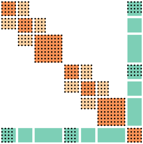
Figure 1: Sparsity structure and detected blocks of $\Psi$ for scenario problem (14) with $M=2$, $N=4$, and $N_{s}=2$.

Importantly, while the sparsity pattern of $\Psi$ depends on the ordering of decision variables, it remains invariant to constraint ordering due to terms $A^{\top}A$ and $G^{\top}(W^{k}+\delta_{k}I_{m})^{-1}G$ that are invariant to row permutations in $A$ and $G$. This characteristic significantly simplifies the user experience, requiring only correct decision variable ordering.

VI Numerical Examples

We benchmark our algorithm against the original PIQP (sparse) [9] solver, the generic QP solvers OSQP [8] and QPALM [21], and the tailored OCP solver HPIPM [10]. To assess the impact of hardware optimization, we evaluate PIQP using both SSE and AVX2 instruction sets. HPIPM is compiled targeting the AVX2 instruction set. All benchmarks are executed on an Intel Core i9 2.4 GHz CPU with Turbo Boost disabled to ensure consistent thermal performance.

Following established literature, we base our numerical experiments on the classical spring-mass system [22], extended with an additional cost term penalizing input differences between consecutive stages. The resulting optimization problem is formulated as

$$\min_{z,u} \sum_{i=0}^{N-1}\ell_{i}(z_{i},u_{i},u_{i+1})+\ell_{N}(z_{N})$$ (13)

s.t. $$z_{0}=\bar{x}_{0},$$

$$z_{i+1}=Az_{i}+Bu_{i},$$

$$-4\cdot\mathbf{1}_{n_{x}}\leq z_{i}\leq 4\cdot\mathbf{1}_{n_{x}},$$

$$-0.5\cdot\mathbf{1}_{n_{u}}\leq u_{i}\leq 0.5\cdot\mathbf{1}_{n_{u}},$$

with stage cost

$$\ell_{i}(z_{i},u_{i},u_{i+1}) =z_{i}^{\top}Qz_{i}+u_{i}^{\top}Ru_{i}$$

$$+\left(u_{i}-u_{i+1}\right)^{\top}R_{d}\left(u_{i}-u_{i+1}\right),$$

and terminal cost $\ell_{N}(z_{N})=z_{N}^{\top}Q_{N}z_{N}$, where $z_{i}\in\mathbb{R}^{n_{x}}$ and $u_{i}\in\mathbb{R}^{n_{u}}$. For a system with $M$ masses, the state dimension is $n_{x}=2M$, with $M-1$ actuators yielding an input dimension of $n_{u}=M-1$. We select cost matrices $Q=10^{3}\cdot I_{n_{x}}$, $R=R_{d}=10^{-1}\cdot I_{n_{u}}$, and derive $Q_{N}$ as the solution from the discrete-time Riccati equation. To exploit the block-tri-diagonal structure in $\Psi$, we organize the decision variables as $x=(z_{0},u_{0},\dots,z_{N-1},u_{N-1},z_{N})$ with no global variables, i.e. $g$ empty.

Following [12], we initialize the system state by sampling $\gamma\sim U[0.5,1.5]$ and subsequently drawing $\bar{x}_{0}\sim U[-\gamma,\gamma]$, ensuring a balanced distribution of active and inactive constraints. All solvers are configured with identical absolute and relative tolerances of $10^{-6}$ and warm-started using zero-input trajectories simulated from $\bar{x}_{0}$.

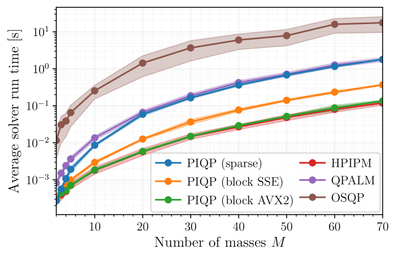
Figure 2: Average solve time and standard dedication over 30 runs for a varying number of masses $M$ for $R_{d}=0$ and $N=15$.

Our initial benchmark considers the case where $R_{d}=0$, eliminating input coupling between stages. For each configuration, we perform 30 runs with the number of masses $M$ ranging from 2 to 70. The results in Figure 2 demonstrate that our new PIQP backend achieves substantial performance improvements: a 13x speed-up compared to the generic sparse backend and up to 245x acceleration versus OSQP. The transition from SSE to AVX2 instructions yields the theoretical 2x performance gain, highlighting the effectiveness of dense kernels and vectorization. For small problem sizes, the vectorization and cache locality of the dense kernels are less advantageous, i.e., the generic sparse interface might even be slightly faster.

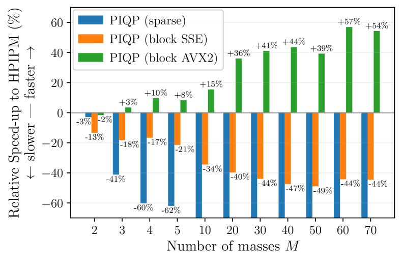
Figure 3: Relative speed-up compared to HPIPM for a varying number of masses $M$ for $R_{d}=10^{-1}\cdot I_{n_{u}}$ and $N=15$.

Introducing input coupling with $R_{d}=10^{-1}\cdot I_{n_{u}}$ challenges the standard OCP structure expected by HPIPM. Similar as in Section IV-B, we address this by augmenting the state to $x_{i}=(z_{i},u_{i},\bar{u}_{i+1})$ with the constraint $\bar{u}_{i}=u_{i}$, effectively decoupling the stages in the cost. Under these conditions, as shown in Figure 3, PIQP outperforms HPIPM by up to 57%.

To evaluate performance with global decision variables $g$, we extend problem (13) to a robust scenario formulation [6]

$$\min_{z,u} \frac{1}{N_{s}}\sum_{j=1}^{N_{s}}\left(\sum_{i=0}^{N-1}\ell_{i}(z_{i}^{j},u_{i}^{j})+\ell_{N}(z_{N}^{j})\right)$$ (14)

s.t. $$z_{0}^{j}=\bar{x}_{0},u_{0}^{1}=u_{0}^{j}$$

$$z^{j}_{i+1}=A^{j}z_{i}^{j}+B^{j}u_{i}^{j},$$

$$-4\cdot\mathbf{1}_{n_{x}}\leq z^{j}_{i}\leq 4\cdot\mathbf{1}_{n_{x}},$$

$$-0.5\cdot\mathbf{1}_{n_{u}}\leq u^{j}_{i}\leq 0.5\cdot\mathbf{1}_{n_{u}},$$

with $N_{s}$ scenarios. The system matrices $A^{j}$ and $B^{j}$ describe $N_{s}$ distinct spring-mass systems, each with spring constants sampled uniformly from $U[1,2]$. Organizing the variables as $x=(z_{1}^{1},u_{1}^{1},\dots,z_{N}^{1},z_{1}^{2},u_{1}^{2},\dots,z_{N}^{N_{s}})$ and $g=(x_{0},u_{0})$ yields the block-tri-diagonal-arrow structure illustrated in Figure 1. The performance comparison between the block-sparse backend using AVX2 instructions and the sparse backend reveals increasing efficiency with problem size, reaching an 8.2x speed-up through improved vectorization, cache utilization, and linear memory access patterns that better utilize available memory bandwidth on modern CPUs.

Figure 4: Speed-up of the block-sparse backend compared to the sparse backend in PIQP for different number of masses $M$, scenarios $N_{s}$ and horizon $N=15$.

References

- [1] L. Vanroye, A. Sathya, J. De Schutter, and W. Decré, “FATROP: A fast constrained optimal control problem solver for robot trajectory optimization and control,” in IEEE/RSJ International Conference on Intelligent Robots and Systems (IROS), 2023, pp. 10 036–10 043.
- [2] J. J. A. Zanelli, A. Domahidi and M. Morari, “FORCES NLP: an efficient implementation of interior-point methods for multistage nonlinear nonconvex programs,” International Journal of Control, vol. 93, no. 1, pp. 13–29, 2020.
- [3] F. Pacaud, M. Schanen, S. Shin, D. A. Maldonado, and M. Anitescu, “Parallel interior-point solver for block-structured nonlinear programs on SIMD/GPU architectures,” Optimization Methods and Software, vol. 39, no. 4, pp. 874–897, 2024.
- [4] S. Shin, M. Anitescu, and F. Pacaud, “Accelerating optimal power flow with GPUs: SIMD abstraction of nonlinear programs and condensed-space interior-point methods,” Electric Power Systems Research, vol. 236, p. 110651, 2024.
- [5] D. Limon, M. Pereira, D. Muñoz de la Peña, T. Alamo, C. N. Jones, and M. N. Zeilinger, “Mpc for tracking periodic references,” IEEE Transactions on Automatic Control, vol. 61, no. 4, pp. 1123–1128, 2016.
- [6] S. Lucia, T. Finkler, and S. Engell, “Multi-stage nonlinear model predictive control applied to a semi-batch polymerization reactor under uncertainty,” Journal of Process Control, vol. 23, no. 9, pp. 1306–1319, 2013.
- [7] D. Limon, I. Alvarado, T. Alamo, and E. Camacho, “MPC for tracking piecewise constant references for constrained linear systems,” Automatica, vol. 44, no. 9, pp. 2382–2387, 2008.
- [8] B. Stellato, G. Banjac, P. Goulart, A. Bemporad, and S. Boyd, “OSQP: An operator splitting solver for quadratic programs,” Mathematical Programming Computation, vol. 12, no. 4, pp. 637–672, 2020.
- [9] R. Schwan, Y. Jiang, D. Kuhn, and C. N. Jones, “PIQP: A proximal interior-point quadratic programming solver,” in IEEE Conference on Decision and Control (CDC), 2023, pp. 1088–1093.
- [10] G. Frison and M. Diehl, “HPIPM: a high-performance quadratic programming framework for model predictive control,” IFAC-PapersOnLine, vol. 53, no. 2, pp. 6563–6569, 2020.
- [11] A. Domahidi, A. U. Zgraggen, M. N. Zeilinger, M. Morari, and C. N. Jones, “Efficient interior point methods for multistage problems arising in receding horizon control,” in IEEE Conference on Decision and Control (CDC), 2012, pp. 668–674.
- [12] K. F. Løwenstein, D. Bernardini, and P. Patrinos, “QPALM-OCP: A Newton-type proximal augmented lagrangian solver tailored for quadratic programs arising in model predictive control,” IEEE Control Systems Letters, vol. 8, pp. 1349–1354, 2024.
- [13] J. Frey, S. Di Cairano, and R. Quirynen, “Active-set based inexact interior point QP solver for model predictive control,” IFAC-PapersOnLine, vol. 53, no. 2, pp. 6522–6528, 2020.
- [14] R. T. Rockafellar, “Augmented Lagrangians and applications of the proximal point algorithm in convex programming,” Mathematics of Operations Research, vol. 1, no. 2, pp. 97–116, 1976.
- [15] S. Pougkakiotis and J. Gondzio, “An interior point-proximal method of multipliers for convex quadratic programming,” Computational Optimization and Applications, vol. 78, no. 2, pp. 307–351, 2021.
- [16] J. Nocedal and S. J. Wright, Numerical Optimization. Springer, 2006.
- [17] R. J. Vanderbei, “Symmetric quasidefinite matrices,” SIAM Journal on Optimization, vol. 5, no. 1, pp. 100–113, 1995.
- [18] G. Frison and J. B. Jørgensen, “Efficient implementation of the Riccati recursion for solving linear-quadratic control problems,” in IEEE International Conference on Control Applications (CCA), 2013, pp. 1117–1122.
- [19] A. Malyshev, R. Quirynen, A. Knyazev, and S. D. Cairano, “A regularized Newton solver for linear model predictive control,” in European Control Conference (ECC), 2018, pp. 1393–1398.
- [20] G. Frison, D. Kouzoupis, T. Sartor, A. Zanelli, and M. Diehl, “BLASFEO: Basic linear algebra subroutines for embedded optimization,” ACM Transactions on Mathematical Software, vol. 44, no. 4, Jul. 2018.
- [21] B. Hermans, A. Themelis, and P. Patrinos, “QPALM: A Newton-type proximal augmented lagrangian method for quadratic programs,” in IEEE Conference on Decision and Control (CDC), 2019, pp. 4325–4330.
- [22] Y. Wang and S. Boyd, “Fast model predictive control using online optimization,” IEEE Transactions on Control Systems Technology, vol. 18, no. 2, pp. 267–278, 2010.