Nonparametric adaptive payload tracking for an offshore crane

Abstract

A nonparametric adaptive crane control system is proposed where the crane payload tracks a desired trajectory with feedback from the payload position. The payload motion is controlled with the position of the crane tip using partial feedback linearization. This is made possible by introducing a novel model structure given in Cartesian coordinates. This Cartesian model structure makes it possible to implement a nonparametric adaptive controller which cancels disturbances by approximating the effects of unknown disturbance forces and structurally unknown dynamics in a reproducing kernel Hilbert space (RKHS). It is shown that the nonparametric adaptive controller leads to uniformly ultimately bounded errors in the presence of unknown forces and unmodeled dynamics. Moreover, it is shown that the Cartesian formulation has certain advantages in payload tracking control also in the non-adaptive case. The performance of the nonparametric adaptive controller is validated in simulation and experiments with good results.

,

1 Introduction

Cranes play a vital role in construction, manufacturing and logistics by enabling efficient handling of heavy loads. Crane control is a challenging problem due to nonlinearities and underactuation, and payload oscillations can lead to inefficiency and hazardous situations. Cranes operating offshore compound these issues as they are exposed to severe wind and ocean wave disturbances. Control systems may offer significant improvements in crane operations, such as enhanced safety, reduced operational costs, and improved efficiency.

1.1 Related work

There is a large body of work on the automatic control of cranes, with extensive reviews presented in [1] and [21]. An early work on crane control is presented in [22] where a linear optimal controller and a state observer are used to control a rotary crane.

Feedforward techniques such as input shaping have been extensively studied for application in crane control. This is done by convolving the input with a series of impulses to reduce the pendulum motion of the payload [8]. Input shaping for a tower crane was used in [4], where the nonlinearities of the system were considered. Flatness-based tracking was used in [13] to control an overhead crane. The controller combined feedforward control and state feedback to reduce payload oscillations and to improve tracking performance. Flatness-based control was also used in [14] to generate and track minimum time trajectories for a gantry crane.

Model predictive control (MPC) has also been applied in crane control. In [12] a hybrid approach was proposed where feedforward control was used with a nonlinear MPC controller to damp payload oscillations on a shipboard crane subject to wave motion. An MPC controller was used in [2] to control a mobile boom crane. The coupled nonlinear dynamic model was linearized along the reference trajectory of the system, approximating the nonlinear optimal control problem using a quadratic programming problem. This allowed for a real-time implementation. This work was extended in [17] for a mobile boom crane to achieve tracking and anti-sway control. The controllers were derived using input/output linearization, and smooth trajectories for the controllers were generated from operator commands using an MPC controller. In [36], nonlinear MPC was used to control an overhead crane, performing point-to-point trajectories while varying the cable length of the crane and canceling disturbances. An MPC controller was proposed in [39] to control a two-dimensional overhead crane while minimizing energy consumption and payload swing angle. In [28], MPC with a particle swarm optimizer was proposed to control an overhead two-dimensional crane, performing tracking control and parameter identification online while limiting the oscillations of the crane payload. A nonlinear MPC controller was combined with a Lyapunov-based damping controller in [34] for tracking control of a knuckle boom crane. The exponentially stabilizing damping controller ensured that the payload oscillation was bounded when the MPC moved the crane suspension point.

Controllers using nonlinear and energy-based control have also been studied for control crane systems. Early work considered two-dimensional overhead or gantry cranes. A nonlinear feedback controller was proposed in [41] for a two-dimensional gantry crane where singular perturbation was used. This led to a composite controller with a slow tracking capability combined with fast oscillation damping. In [40], a two-dimensional gantry crane with constrained pendulum length and trolley motion was controlled using a Lyapunov-based nonlinear controller. LaSalle’s invariance principle was used in [9] to design a PD controller for tracking control of a two-dimensional overhead crane. This paper also included two nonlinear controllers based on PD control, where tracking and payload oscillation damping were improved by including nonlinear terms to account for coupling effects. An energy-based stabilizing feedback controller was presented in [32] for a 4-DOF overhead crane for trolley position control and payload oscillation damping subject to input constraints. Nonlinear tracking control and swing damping of a three-dimensional overhead crane was proposed in [38] using a feedback linearization approach. In [7] an energy-based controller was proposed for damping the payload oscillations of a bifilar overhead crane. In [33], a controller was proposed for a knuckle boom crane using vision-based feedback. The controller used an inner damping control loop to cancel payload oscillations and an outer PD controller to translate the crane suspension point. The vision system was used to estimate the payload oscillation angles and the crane cable length.

Learning-based and adaptive methods have also been applied to crane control to compensate for model uncertainties and disturbance forces. To deal with model uncertainties, [30] proposed an energy-based adaptive controller for a planar overhead crane. The controller tracked the desired trolley position and cable length while damping payload oscillations and estimating the payload mass. In [31], an adaptive controller was proposed for automatic control of a tower crane under model uncertainties for position control and to limit payload oscillations. An adaptive controller was proposed in [19] where a learning algorithm was used to control a two-dimensional offshore boom crane subject to wave disturbances. The learning algorithm assumed a periodic structure to the wave disturbance. The adaptive algorithm was used to compensate for disturbances by estimating unknown system parameters and the wave period.

Crane control systems have largely been based on accurate control of the suspension point in combination with damping of the payload pendulum motion, as in [34]. In this paper, a different approach is used where the focus is on tracking control of payload motion with feedback from the payload position, e.g., using camera measurements. This has the potential of higher accuracy and faster response for payload motion tracking. The performance of the proposed control system is further improved by introducing a nonparametric adaptive controller.

In this paper we propose a crane control system for tracking control of payload motion by using the novel nonparametric adaptive controller introduced in [5]. This adaptive controller models the disturbance term as an element in an RKHS, which means that the learning is data-driven. To apply this adaptive controller, it was necessary to reformulate the dynamic model used in [34], where Euler angles were used, to a model in Cartesian coordinates and then to apply partial feedback linearization [29] for this Cartesian model. This Cartesian model can also be used to achieve high-performance tracking in the nonadaptive case, as demonstrated in this paper. It is shown with Lyapunov-like analysis that the proposed controller gives uniformly ultimately bounded tracking errors and that the controller handles disturbances due to disturbance forces and unmodeled effects.

1.2 Contribution

The contributions of the paper are:

1. A novel Cartesian model of the combined crane and payload dynamics is formulated by a change of coordinates from the usual model with Euler angles.

2. Partial feedback linearization is formulated for the Cartesian model, and it is shown that the payload can be controlled with the position of the crane tip instead of the acceleration of the crane tip.

3. It is shown that partial feedback linearization with the Cartesian model has certain advantages for payload tracking compared to partial feedback linearization with the Euler angle model.

4. It is shown how to apply the nonparametric adaptive controller of [5] to the Cartesian model with partial feedback linearization, and stability properties are analyzed with and without the saturation function used in [5].

5. The nonparametric adaptive controller is validated with good results in simulations and experiments where the base of the crane has a significant sinusoidal motion similar to a wave excitation on a ship. The disturbance was significantly reduced and the tracking performance was significantly improved with the adaptive compensation.

1.3 Paper structure

This paper is organized as follows. The problem formulation and theoretical preliminaries are presented in Section 2. The Cartesian model for the crane is developed in Section 3. The control design is presented in Section 4. The simulation studies and experimental validation are presented in Section 5. Finally, the conclusion is presented in Section 6.

2 Problem formulation

2.1 Crane model

The nonparametric adaptive controller was applied to a novel dynamic model of the crane payload dynamics given in Cartesian coordinates. This model is given by

$$\ddot{x}+\omega_{0}^{2}\frac{L_{z}}{L}x =\omega_{0}^{2}\frac{L_{z}}{L}x_{0}+n_{x}+\sigma_{x}$$ (1)

$$\ddot{y}+\omega_{0}^{2}\frac{L_{z}}{L}y =\omega_{0}^{2}\frac{L_{z}}{L}y_{0}+n_{y}+\sigma_{y}$$ (2)

Here $(x,y)$ is the position of the payload and $(x_{0},y_{0})$ is the position of the suspension point at the crane tip, $L$ is the constant length of the crane cable, $L_{z}$ is the vertical distance from the crane tip to the cane load, $\omega_{0}=\sqrt{g/L}$, $n_{x}$ and $n_{y}$ are higher order modeling terms and $\sigma_{x}$ and $\sigma_{y}$ are generalized disturbance forces. This model structure was introduced since it allows for the use of the position $(x_{0},y_{0})$ of the suspension point as the control variable for the payload motion. This is done in a solution where the crane tip is controlled by partial feedback linearization [29]. As will be shown in the following, this model structure is well suited for the application of the nonparametric adaptive controller of [5].

In Section 3 it is shown how the dynamic model (1, 2) can be derived from the well-established dynamic model in Euler angles [34]:

$$\ddot{\phi}_{x}c_{y}+\omega_{0}^{2}s_{x} =\frac{c_{x}}{L}\ddot{y}_{0}+n_{\phi_{x}}+\sigma_{\phi_{x}}$$ (3)

$$\ddot{\phi}_{y}+\omega_{0}^{2}c_{x}s_{y} =-\frac{c_{x}}{L}\ddot{x}_{0}+n_{\phi_{y}}+\sigma_{\phi_{y}}$$ (4)

Here $\phi_{x}$ and $\phi_{y}$ are the Euler angles of the cable, $c_{x}=\cos\phi_{x}$, $s_{x}=\sin\phi_{x}$, $c_{y}=\cos\phi_{y}$, $s_{y}=\sin\phi_{y}$ and $n_{\phi_{x}}$ and $n_{\phi_{y}}$ are higher order modeling terms and $\sigma_{\phi_{x}}$ and $\sigma_{\phi_{y}}$ are generalized disturbance forces. In this case, the acceleration $(\ddot{x}_{0},\ddot{y}_{0})$ of the suspension point can be used as the control variable for damping the pendulum motion of the load. In [34], this was done by controlling the crane tip with partial feedback linearization and then using the acceleration of the crane tip to damp out the pendulum motion of the load. We found that this model in Euler angles was not straightforward to use with the nonparametric adaptive controller.

2.2 Reproducing kernel Hilbert space

Methods based on reproducing kernel Hilbert spaces (RKHS) [3] are well established for data-driven identification of unknown functions [18]. In this paper we use the nonparametric adaptive controller proposed in [5], where an RKHS formulation is used to approximate an unknown disturbance. A brief introduction to RKHS is presented in the following based on [15] and [16].

Let ${{\bm{K}}:{\mathbb{R}}^{n}\times{\mathbb{R}}^{n}\rightarrow{\mathbb{R}^{m\times m}}}$ be a matrix-valued reproducing kernel. Then the kernel will be positive definite in the sense that ${\bm{K}}({\bm{x}},{\bm{z}})={\bm{K}}({\bm{z}},{\bm{x}})^{\text{T}}$ for all ${\bm{x}},{\bm{z}}\in{\mathbb{R}}^{n}$ and

$$\sum_{i=1}^{N}\sum_{j=1}^{N}\left\langle{\bm{a}}_{i},{\bm{K}}({\bm{x}}_{i},{\bm{x}}_{j}){\bm{a}}_{j}\right\rangle\geq 0$$ (5)

for any sets of vectors ${\{{\bm{x}}_{i}\}_{i=1}^{N}\in{\mathbb{R}}^{n}}$, ${\{{\bm{a}}_{i}\}_{i=1}^{N}\in{\mathbb{R}}^{m}}$ and for any integrer $N>0$. Define the function ${{\bm{K}}_{x}{\bm{a}}:{\mathbb{R}}^{n}\rightarrow{\mathbb{R}}^{m}}$ by

$$({\bm{K}}_{x}{\bm{a}})({\bm{z}})={\bm{K}}({\bm{z}},{\bm{x}}){\bm{a}}\in{\mathbb{R}}^{m}$$ (6)

for all ${\bm{a}}\in{\mathbb{R}}^{m}$ and ${\bm{x}},{\bm{z}}\in{\mathbb{R}}^{n}$. Then the reproducing kernel ${\bm{K}}$ defines the RKHS ${\mathcal{H}_{K}}$ given by

$$\mathcal{H}_{K}=\overline{\operatorname{span}}\{{\bm{K}}_{x}{\bm{a}}\;|\;{\bm{x}}\in{\mathbb{R}}^{n},{\bm{a}}\in{\mathbb{R}}^{m}\}$$ (7)

It follows that for any function ${\bm{f}}\in\mathcal{H}_{K}$ there will be sets of vectors ${\{{\bm{x}}_{i}\}_{i=1}^{\infty}\in{\mathbb{R}}^{n}}$, ${\{{\bm{a}}_{i}\}_{i=1}^{\infty}\in{\mathbb{R}}^{m}}$ so that

$${\bm{f}}({\bm{x}})=\sum_{i=1}^{\infty}({\bm{K}}_{x_{i}}{\bm{a}}_{i})({\bm{x}})=\sum_{i=1}^{\infty}{\bm{K}}({\bm{x}},{\bm{x}}_{i}){\bm{a}}_{i}$$ (8)

The reproducing kernel function can be expressed in terms of a feature map $\bm{\Phi}({\bm{x}})$ as ${\bm{K}}({\bm{x}},{\bm{z}})=\bm{\Phi}({\bm{x}})^{\text{T}}\bm{\Phi}({\bm{z}})$.

Suppose that the kernel ${\bm{K}}$ is shift invariant, which means that ${\bm{K}}({\bm{x}},{\bm{z}})={\bm{G}}({\bm{x}}-{\bm{z}})$ where ${\bm{G}}$ is called the signature of ${\bm{K}}$. Then from the vector version of Brochner’s theorem there is a matrix function ${\bm{B}}({\bm{w}})$ and a probability density function $p({\bm{w}})$ so that [6]

$${\bm{K}}({\bm{x}},{\bm{z}}) =\int_{{\mathbb{R}}^{d}}e^{i({\bm{x}}-{\bm{z}})^{\text{T}}{\bm{w}}}{\bm{B}}({\bm{w}}){\bm{B}}({\bm{w}})^{*}p({\bm{w}})d{\bm{w}}$$

$$=\int_{{\mathbb{R}}^{d}}\bm{\Psi}_{b}({\bm{x}},{\bm{w}})^{*}\bm{\Psi}_{b}({\bm{z}},{\bm{w}})p({\bm{w}})d{\bm{w}}$$ (9)

where

$$\bm{\Psi}_{b}({\bm{x}},{\bm{w}})=\begin{bmatrix}\cos({\bm{w}}^{{\text{T}}}{\bm{x}})\\ \sin({\bm{w}}^{{\text{T}}}{\bm{x}})\end{bmatrix}{\bm{B}}({\bm{w}})^{*}$$ (10)

A random Fourier feature (RFF) approximation [6, 20] of the kernel is then

$${\bm{K}}({\bm{x}},{\bm{z}})\approx\sum_{j=1}^{d}\ \bm{\Psi}_{b}({\bm{x}},{\bm{w}}_{j})^{*}\bm{\Psi}_{b}({\bm{z}},{\bm{w}}_{j})$$ (11)

where ${\bm{w}}_{1},\ldots,{\bm{w}}_{d}$ are drawn i.i.d. with probability $p({\bm{w}})$. The number of random features ${d}$ is chosen to balance the quality of the approximation with respect to the computational requirements. The RFF approximation of the function ${\bm{f}}\in\mathcal{H}_{K}$ in (8) is then

$${\bm{f}}({\bm{x}}) \approx\sum_{i=1}^{\infty}\sum_{j=1}^{d}\ \left(\bm{\Psi}_{b}({\bm{x}},{\bm{w}}_{j})^{*}\bm{\Psi}_{b}({\bm{x}}_{i},{\bm{w}}_{j})\right){\bm{a}}_{i}$$ (12)

This gives the finite-dimensional approximation

$${\bm{f}}({\bm{x}})\approx\sum_{j=1}^{d}\bm{\Psi}_{b}({\bm{x}},{\bm{w}}_{j})^{*}\bm{\alpha}_{j}$$ (13)

where $\bm{\alpha}_{j}=\sum_{i=1}^{\infty}\bm{\Psi}_{b}({\bm{x}}_{i},{\bm{w}}_{j}){\bm{a}}_{i}\in{\mathbb{R}}^{m}$. It is noted that $\bm{\alpha}_{j}$ will be found by optimization in regression problems or from an adaptive control law in the nonparametric controller, which means that the vectors ${\bm{a}}_{1},{\bm{a}}_{2},\ldots$ and the infinite sum are not calculated. A uniform upper bound for the approximation error in (13) can be derived.

2.3 Gaussian separable kernel

In this paper, the Gaussian separable kernel [26] will be used. This is a reproducing kernel which is shift invariant and given by

$${\bm{K}}_{\sigma}({\bm{x}},{\bm{z}})=k_{\sigma}({\bm{x}},{\bm{z}}){\bm{I}}_{m}\in{\mathbb{R}^{m\times m}}$$ (14)

where ${\bm{I}}_{m}\in{\mathbb{R}^{m\times m}}$ is the identity matrix and

$$k_{\sigma}({\bm{x}},{\bm{z}})=e^{\left(-\frac{\|{\bm{x}}-{\bm{z}}\|^{2}}{2\sigma^{2}}\right)}=e^{-\frac{\|{\bm{x}}\|^{2}}{2\sigma^{2}}}e^{-\frac{\|{\bm{z}}\|^{2}}{2\sigma^{2}}}e^{\frac{{\bm{x}}^{\text{T}}{\bm{z}}}{\sigma^{2}}}$$ (15)

is the scalar Gaussian kernel with kernel width ${\sigma>0}$. The Gaussian kernel has an infinite-dimensional feature map, which is seen from (15), where the term $\exp\left({\bm{x}}^{\text{T}}{\bm{z}}/\sigma^{2}\right)$ must be represented by an infinite series in a factorization. This is shown in Appendix A. In this case (9) holds with ${\bm{B}}={\bm{I}}_{m}$ and $p({\bm{w}})=\mathcal{N}({\bm{0}},\sigma^{-2}{\bm{I}}_{n})$. The approximations (11) and (13) can be written as [26, 27]

$${\bm{K}}_{\sigma}({\bm{x}},{\bm{z}})\approx\bm{\Psi}({\bm{x}})^{{\text{T}}}\bm{\Psi}({\bm{z}})$$ (16)

and

$${\bm{f}}({\bm{x}})\approx\bm{\Psi}({\bm{x}})^{{\text{T}}}\bm{\alpha}$$ (17)

where $\bm{\alpha}=\in{\mathbb{R}}^{2dm}$,

$$\bm{\Psi}({\bm{x}})=\bm{\psi}({\bm{x}})\otimes{\bm{I}}_{m}\in{\mathbb{R}}^{2dm\times m}$$ (18)

where $\otimes$ is the Kronecker product, and

$$\bm{\psi}({\bm{x}})=\frac{1}{\sqrt{d}}\begin{bmatrix}\cos({\bm{w}}_{1}^{{\text{T}}}{\bm{x}})\\ \sin({\bm{w}}_{1}^{{\text{T}}}{\bm{x}})\\ \vdots\\ \cos({\bm{w}}_{d}^{{\text{T}}}{\bm{x}})\\ \sin({\bm{w}}_{d}^{{\text{T}}}{\bm{x}})\end{bmatrix}\in{\mathbb{R}}^{2d}$$ (19)

where ${d>0}$ is the number of random features. The weights ${{\bm{w}}_{1},\dots,{\bm{w}}_{d}\in{\mathbb{R}}^{n}}$ are drawn i.i.d. with distribution ${{\mathcal{N}}\left({\bm{0}},\sigma^{-2}{\bm{I}}_{n}\right)}$.

2.4 Nonparametric adaptive controller

In this paper, the nonparametric adaptive controller of [5] is used for tracking control of the crane payload. This controller was developed in [5] for the nonlinear system

$$\dot{\bm{x}}={\bm{f}}({\bm{x}},t)+{\bm{B}}({\bm{x}},t)({\bm{u}}({\bm{x}},t)-{\bm{h}}({\bm{x}}))$$ (20)

where ${{\bm{x}}\in{\mathbb{R}}^{n}}$ is the system state, ${t\in{\mathbb{R}}_{\geq 0}}$ is time, ${\bm{f}}:{\mathbb{R}}^{n}\times{\mathbb{R}}_{\geq 0}\rightarrow{\mathbb{R}}^{n}$ are the nominal dynamics, ${\bm{B}}:{\mathbb{R}}^{n}\times{\mathbb{R}}_{\geq 0}\rightarrow{\mathbb{R}}^{n\times m}$ is the control matrix, ${{\bm{u}}:{\mathbb{R}}^{n}\times{\mathbb{R}}_{\geq 0}\rightarrow{\mathbb{R}}^{m}}$ is the learned control input, and ${\bm{h}}:{\mathbb{R}}^{n}\rightarrow{\mathbb{R}}^{m}$ is the unknown disturbance term, which is assumed to be an element of the RKHS $\mathcal{H}_{K}$, which is defined by the reproducing kernel ${\bm{K}}:{\mathbb{R}}^{n}\times{\mathbb{R}}^{n}\rightarrow{\mathbb{R}^{m\times m}}$ with a feature map $\bm{\Phi}({\bm{x}})$ which satisfies ${\bm{K}}({\bm{x}},{\bm{z}})=\bm{\Phi}({\bm{x}})^{\text{T}}\bm{\Phi}({\bm{z}})$. It is noted that the feature map $\bm{\Phi}({\bm{x}})$ is infinite-dimensional for the Gaussian kernel.

The tracking error ${{\bm{e}}\in{\mathbb{R}}^{n}}$ is defined as ${{\bm{e}}={\bm{x}}-{\bm{x}}_{d}}$ where ${{\bm{x}}_{d}\in{\mathbb{R}}^{n}}$ is the desired trajectory. The error dynamics are assumed to be given by

$$\dot{\bm{e}}={\bm{f}}_{e}({\bm{e}},t)+{\bm{B}}({\bm{x}},t)({\bm{u}}({\bm{x}},t)-{\bm{h}}({\bm{x}}))$$ (21)

where nominal error dynamics $\dot{\bm{e}}={\bm{f}}_{e}({\bm{e}},t)$ are exponentially stable. This implies that there exists a continuously differentiable function ${Q:{\mathbb{R}}^{n}\times{\mathbb{R}}_{\geq 0}\rightarrow{\mathbb{R}}}$ such that

$$k_{1}\|{\bm{e}}\|^{a}\leq Q({\bm{e}},t)\leq k_{2}\|{\bm{e}}\|^{a}$$ (22)

and the time derivative of ${Q({\bm{e}},t)}$ along the trajectories of the nominal error dynamics satisfies

$$\left\langle\nabla Q({\bm{e}},t),{\bm{f}}_{e}({\bm{e}},t)\right\rangle+\frac{\partial Q}{\partial t}({\bm{e}},t)\leq-k_{3}\|{\bm{e}}\|^{a}$$ (23)

where $k_{1}$, $k_{2}$, $k_{3}$, and $a$ are positive constants [11].

An adaptive control law which compensates for the unknown disturbance ${\bm{h}}({\bm{x}})$ in (21) is given by

$${\bm{u}}({\bm{x}},t)=\hat{{\bm{h}}}({\bm{x}},t)$$ (24)

where $\hat{{\bm{h}}}(\cdot,t)$ is an estimate of ${\bm{h}}\in\mathcal{H}_{K}$. In the nonparametric adaptive controller of [5] the estimate is given by

$$\hat{{\bm{h}}}({\bm{x}},t) =\int_{0}^{t}{\bm{K}}({\bm{x}},{\bm{x}}(\tau)){\bm{c}}(\tau)d\tau$$ (25)

$${\bm{c}}(t) =-\gamma{\bm{B}}_{e}({\bm{x}},t)^{{\text{T}}}\nabla Q({\bm{e}},t)$$ (26)

To compare the adaptive control law (25, 26) to a conventional adaptive control law like the one in [23] it is useful to define the parameter vector estimate

$$\hat{\bm{\beta}}(t)=-\gamma\int_{0}^{t}\bm{\Phi}({\bm{x}}(\tau)){\bm{B}}_{e}({\bm{x}}(\tau),\tau)^{\text{T}}\nabla Q({\bm{e}}(\tau),\tau)d\tau$$

It is then straightforward to see that the adaptive control law (25, 26) is equivalent to

$$\hat{{\bm{h}}}({\bm{x}},t) =\bm{\Phi}({\bm{x}})^{{\text{T}}}\hat{\bm{\beta}}(t)$$ (27)

$$\dot{\hat{\bm{\beta}}} =-\gamma\bm{\Phi}({\bm{x}}){\bm{B}}({\bm{x}},t)^{{\text{T}}}\nabla Q({\bm{e}},t)$$ (28)

where $\bm{\Phi}$ and $\hat{\bm{\beta}}$ are of infinite dimension. The use of the kernel function in (25) to have an adaptive control law that is effectively infinite-dimensional is referred to as an application of the kernel trick in [5]. The adaptive controller guarantees the existence and uniform boundedness of ${{\bm{x}}(t)}$ and ${{\bm{e}}(t)}$, and that ${\bm{u}}(\cdot,t)\in\mathcal{H}_{K}$ for all ${t\geq 0}$, and that the error signal satisfies $\lim_{t\rightarrow\infty}\|{\bm{e}}(t)\|_{2}=0$ [5, Theorem 4.5].

The computational requirements of the adaptive control law (25, 26) do not allow for real-time computation. This is problem is solved in [5] by using an RFF approximation of the kernel. The function ${\bm{h}}\in\mathcal{H}_{K}$ is then approximated as in (17), which gives

$${\bm{h}}({\bm{x}})=\bm{\Psi}({\bm{x}})^{{\text{T}}}{\bm{\alpha}}+{\bm{\epsilon}}$$ (29)

where the approximation error ${\bm{\epsilon}}\in{\mathbb{R}}^{m}$ is bounded by $\|{\bm{\epsilon}}\|\leq B_{\epsilon}$ for some $B_{\epsilon}>0$ [5]. The RFF approximation of the nonparametric adaptive control law (25, 26) is then given by

$$\hat{{\bm{h}}}({\bm{x}},t) =\bm{\Psi}({\bm{x}})^{{\text{T}}}\hat{\bm{\alpha}}(t)$$ (30)

$$\dot{\hat{\bm{\alpha}}} =-\gamma\bm{\Psi}({\bm{x}}){\bm{B}}({\bm{x}},t)^{{\text{T}}}\nabla Q({\bm{e}},t)$$ (31)

where $\bm{\Psi}({\bm{x}})\in{\mathbb{R}}^{2dm\times m}$ and $\bm{\alpha}\in{\mathbb{R}}^{2dm}$ for the Gaussian kernel. The control law (30, 31) can be computed in real time.

The compensation ${\bm{u}}({\bm{x}},t)=\hat{{\bm{h}}}({\bm{x}},t)$ gives

$${\bm{u}}-{\bm{h}}=\bm{\Psi}({\bm{x}})^{{\text{T}}}{\tilde{{\bm{\alpha}}}}+{\bm{\epsilon}}$$ (32)

where ${\tilde{{\bm{\alpha}}}}=\hat{{\bm{\alpha}}}-{\bm{\alpha}}$ is the parameter estimation error. It is noted that the RFF approximation of the nonparametric adaptive controller gives an adaptive controller with a bounded approximation error in $\mathcal{H}_{K}$.

3 Modeling

3.1 Payload dynamics in Euler angles

Let ${n}$ be the inertial frame with origin at the base of the crane and the ${z}$-axis vertically up. Let ${b}$ be the moving frame with origin at ${\bm{r}}_{0}=[x_{0},y_{0},z_{0}]^{\rm T}$, which is the position of the suspension point of the cable in the $n$ frame, and with the ${z}$-axis along the cable. The rotation from frame ${n}$ to frame ${b}$ is given by the rotation matrix ${{\bm{R}}_{b}^{n}={\bm{R}}_{x}(\phi_{x}){\bm{R}}_{y}(\phi_{y})}$ where ${\bm{R}}_{x}$ and ${\bm{R}}_{y}$ are the rotation matrices about the $x$ and $y$ axes and $\phi_{x}$ and $\phi_{y}$ are the angles of rotation [25]. The position of the load mass in the $n$ frame is ${\bm{r}}={\bm{r}}_{0}-{\bm{R}}^{n}_{b}[0,0,L]^{\rm T}$ with coordinates ${\bm{r}}=[x,y,z]^{\rm T}$, and the relative position of the mass with respect to the crane tip is ${\bm{r}}_{r}={\bm{r}}-{\bm{r}}_{0}$ with coordinates ${\bm{r}}_{r}=[x_{r},y_{r},z_{r}]^{\text{T}}$. The constant length of the massless cable is

$$L=\sqrt{x_{r}^{2}+y_{r}^{2}+z_{r}^{2}}$$ (33)

It is assumed that the suspension point moves in the horizontal plane. The equations of motion for the load mass are derived with Kane’s equations of motion in [34, eq. (7)] and are given by

$$\ddot{\phi}_{x}c_{y}+\omega_{0}^{2}s_{x} =-\frac{1}{L}\ddot{y}_{0}c_{x}+2\dot{\phi}_{x}\dot{\phi}_{y}s_{y}+\frac{c_{x}}{mL}F_{y}$$ (34)

$$\ddot{\phi}_{y}+\omega_{0}^{2}c_{x}s_{y} =\frac{1}{L}\ddot{x}_{0}c_{y}+\frac{1}{L}\ddot{y}_{0}s_{x}s_{y}-\dot{\phi}_{x}^{2}s_{y}c_{y}$$

$$\quad-\frac{c_{y}}{mL}F_{x}-\frac{s_{x}s_{y}}{mL}F_{y}$$ (35)

where ${\omega_{0}^{2}=g/L}$ and the notation ${s_{i}=\sin\phi_{i}}$ and ${c_{i}=\cos\phi_{i}}$ is used. The angular motion can then be controlled with the accelerations $(\ddot{x}_{0},\ddot{y}_{0})$ of the suspension point as in [35].

3.2 Payload dynamics in Cartesian coordinates

A change of generalized coordinates from the Euler angles $(\phi_{x},\phi_{y})$ to the Cartesian coordinates $(x,y)$ of the payload is done with the relative positions

$$\begin{bmatrix}x_{r}\\ y_{r}\\ z_{r}\end{bmatrix}=\begin{bmatrix}-s_{y}L\\ s_{x}c_{y}L\\ -c_{x}c_{y}L\end{bmatrix}$$ (36)

as the starting point. It is assumed that $z_{r}<0$, which means that the load is below the suspension point. Then

$$L_{z}=-z_{r}=\sqrt{L^{2}-x_{r}^{2}-y_{r}^{2}}\geq 0$$ (37)

The relative horizontal velocities are then given by

$$\dot{x}_{r} =-\dot{\phi}_{y}c_{y}L$$ (38)

$$\dot{y}_{r} =\dot{\phi}_{x}c_{x}c_{y}L-\dot{\phi}_{y}s_{x}s_{y}L$$ (39)

while the relative horizontal accelerations are

$$\ddot{x}_{r} =-\ddot{\phi}_{y}c_{y}L+\dot{\phi}_{y}^{2}s_{y}L$$ (40)

$$\ddot{y}_{r} =\ddot{\phi}_{x}c_{x}c_{y}L-\ddot{\phi}_{y}s_{x}s_{y}L-\dot{\phi}_{x}^{2}s_{x}c_{y}L$$

$$\quad-\dot{\phi}_{y}^{2}s_{x}c_{y}L-2\dot{\phi}_{x}\dot{\phi}_{y}c_{x}s_{y}L$$ (41)

The equations of motion in the Cartesian coordinates $(x,y)$ are then found by solving for $\ddot{\phi}_{x}$, $\ddot{\phi}_{y}$, $\dot{\phi}_{x}$, $\dot{\phi}_{y}$, $c_{x}$, $s_{x}$, $c_{y}$ and $s_{y}$ from (36–41) and inserting the expressions into the equations of motion (34, 35). A detailed derivation of the Cartesian model is presented in Appendix B. This gives the model

$$\ddot{x}+\Omega_{z}^{2}x =\Omega_{z}^{2}x_{0}+n_{ax}+n_{vx}+\sigma_{x}$$ (42)

$$\ddot{y}+\Omega_{z}^{2}y =\Omega_{z}^{2}y_{0}+n_{ay}+n_{vy}+\sigma_{y}$$ (43)

where $\Omega_{z}^{2}=\omega_{0}^{2}\frac{L_{z}}{L}\leq\omega_{0}^{2}$. The acceleration terms are

$$n_{ax} =\frac{x_{r}^{2}}{L^{2}}\ddot{x}_{0}+\frac{x_{r}y_{r}}{L^{2}}\ddot{y}_{0}$$ (44)

$$n_{ay} =\frac{y_{r}^{2}}{L^{2}}\ddot{y}_{0}+\frac{x_{r}y_{r}}{L^{2}}\ddot{x}_{0}$$ (45)

The velocity-related terms are

$$\begin{split}n_{vx}&=-\frac{x_{r}\dot{x}_{r}^{2}}{L^{2}-x_{r}^{2}}-\frac{x_{r}^{3}y_{r}^{2}\dot{x}_{r}^{2}}{L^{2}L_{z}^{2}(L^{2}-x_{r}^{2})}\\ &\quad-2\frac{x_{r}^{2}y_{r}\dot{x}_{r}\dot{y}_{r}}{L^{2}L_{z}^{2}}-\frac{x_{r}(L^{2}-x_{r}^{2})\dot{y}_{r}^{2}}{L^{2}L_{z}^{2}}\end{split}$$ (46)

$$\begin{split}n_{vy}&=-\frac{y_{r}\dot{x}_{r}^{2}}{L^{2}-x_{r}^{2}}-\frac{x_{r}^{2}y_{r}^{3}\dot{x}_{r}^{2}}{L^{2}L_{z}^{2}(L^{2}-x_{r}^{2})}\\ &\quad-2\frac{x_{r}y_{r}^{2}\dot{x}_{r}\dot{y}_{r}}{L^{2}L_{z}^{2}}-\frac{y_{r}(L^{2}-x_{r}^{2})\dot{y}_{r}^{2}}{L^{2}L_{z}^{2}}\end{split}$$ (47)

and disturbance forces $F_{x}$ and $F_{y}$ in the $x$ and $y$ directions of the $n$ frame result in the terms

$$\sigma_{x} =\frac{y_{r}^{2}+z_{r}^{2}}{mL^{2}}F_{x}-\frac{x_{r}y_{r}}{mL^{2}}F_{y}$$ (48)

$$\sigma_{y} =-\frac{x_{r}y_{r}}{mL^{2}}F_{x}+\frac{x_{r}^{2}+z_{r}^{2}}{mL^{2}}F_{y}$$ (49)

The equations of motion (42, 43) can be controlled with the position $(x_{0},y_{0})$ of the suspension point. The equations (42, 43) have more terms and appear to be more complicated than the equations of motion (34, 35) in Euler angles. However, all terms in $n_{ax}$, $n_{ay}$, $n_{vx}$ and $n_{vy}$ are higher order terms that can be treated as vanishing perturbations in a controller design where the nominal dynamics are exponentially stable [11]. Therefore, these terms are handled without much complication in the controller design used in this paper.

4 Control design

4.1 Partial feedback linearization

Partial feedback linearization [29] is presented in this section for the system consisting of the actuated crane and the unactuated crane load as in [34]. The idea is to control the crane tip with an exponentially stable controller, and then to use the position of the crane tip as the control input to the crane load dynamics. The main change from [34] is that the load model is given in Cartesian coordinates, and is controlled with the tip position, while in [34] Euler angles were used and the load was controlled with the crane tip acceleration.

The generalized coordinates of the crane and the load are ${\bm{q}}=[{\bm{q}}_{1}^{\text{T}},{\bm{q}}_{2}^{\text{T}}]^{\text{T}}$ where ${\bm{q}}_{1}=[\phi_{x},\phi_{y}]^{\text{T}}$ are the Euler angles of the load and ${\bm{q}}_{2}=[q_{1},q_{2},q_{3}]^{\text{T}}$ are the joint angles of the crane. The corresponding input generalized forces of the crane are $\bm{\tau}=[\tau_{1},\tau_{2},\tau_{3}]^{\text{T}}$. The dynamics are given by the underactuated system

$${\bm{M}}_{11}\ddot{\bm{q}}_{1}+{\bm{M}}_{12}\ddot{\bm{q}}_{2}+{\bm{c}}_{q1}+{\bm{g}}_{q1} =\bm{\sigma}_{q}$$ (50)

$${\bm{M}}_{21}\ddot{\bm{q}}_{1}+{\bm{M}}_{22}\ddot{\bm{q}}_{2}+{\bm{c}}_{q2}+{\bm{g}}_{q2} =\bm{\tau}_{q}$$ (51)

where ${\bm{c}}_{q1}={\bm{C}}_{1}({\bm{q}},\dot{\bm{q}})\dot{\bm{q}}$ and ${\bm{c}}_{q2}={\bm{C}}_{2}({\bm{q}},\dot{\bm{q}})\dot{\bm{q}}$ are centrifugal and Coriolis terms, and ${\bm{g}}_{q1}$ and ${\bm{g}}_{q2}$ are gravitational terms. The term $\bm{\sigma}_{q}$ is an unknown generalized disturbance force acting on the load. The elements of ${\bm{M}}_{12}={\bm{M}}_{21}^{\rm T}$ are bounded and $\|{\bm{c}}_{q1}\|\leq C_{n1}\|\dot{\bm{q}}\|^{2}$ where $C_{n1}>0$ is a constant [10]. Here (50) is a reformulation of (34, 35), while (51) is found as standard manipulator dynamics [25].

A change of variables to ${\bm{p}}=[{\bm{y}}^{\rm T},{\bm{y}}_{0}^{\rm T}]^{\rm T}$ where ${\bm{y}}=[x,y]^{\text{T}}$ and ${\bm{y}}_{0}=[x_{0},y_{0}]^{\text{T}}$ is done. The velocity mappings are $\dot{\bm{y}}={\bm{J}}_{1}({\bm{q}}_{1})\dot{\bm{q}}_{1}$ and $\dot{\bm{y}}_{0}={\bm{J}}_{2}({\bm{q}}_{2})\dot{\bm{q}}_{2}$. The dynamics are

$$\ddot{\bm{y}}+{\bm{D}}_{12}\ddot{\bm{y}}_{0}+{\bm{c}}_{1}+{\bm{g}}_{1} =\bm{\sigma}$$ (52)

$${\bm{D}}_{21}\ddot{\bm{y}}+{\bm{D}}_{22}\ddot{\bm{y}}_{0}+{\bm{c}}_{2}+{\bm{g}}_{2} =\bm{\tau}$$ (53)

where (52) follows from (42) and (43), which means that ${\bm{D}}_{11}={\bm{I}}$, ${\bm{c}}_{1}=[n_{vx},n_{vy}]^{\text{T}}$, $\bm{\sigma}=[\sigma_{x},\sigma_{y}]^{\text{T}}$,

$${\bm{g}}_{1}=-\Omega_{z}^{2}({\bm{y}}_{0}-{\bm{y}})$$ (54)

and

$${\bm{D}}_{12}={\bm{D}}_{21}=\begin{bmatrix}\frac{x_{r}^{2}}{L^{2}}&\frac{x_{r}y_{r}}{L^{2}}\\ \frac{x_{r}y_{r}}{L^{2}}&\frac{y_{r}^{2}}{L^{2}}\end{bmatrix}$$ (55)

It follows that ${\bm{D}}_{21}$ is bounded with finite induced norm $B_{12}=\|{\bm{D}}_{21}\|$. Moreover, ${\bm{c}}_{1}={\bm{J}}_{1}^{{-\text{T}}}{\bm{c}}_{q1}$, ${\bm{g}}_{1}={\bm{J}}_{1}^{{-\text{T}}}{\bm{g}}_{q1}$, $\bm{\sigma}={\bm{J}}_{1}^{{-\text{T}}}\bm{\sigma}_{q}$, ${\bm{c}}_{2}={\bm{J}}_{2}^{{-\text{T}}}{\bm{c}}_{q1}$, ${\bm{g}}_{2}={\bm{J}}_{2}^{{-\text{T}}}{\bm{g}}_{q2}$ and $\bm{\tau}={\bm{J}}^{-\text{T}}({\bm{q}}_{2})\bm{\tau}_{q}$. The matrices ${\bm{J}}$ and ${\bm{J}}^{-1}$ are assumed to be bounded, therefore

$$\|{\bm{c}}_{1}\|\leq C_{c1}\|\dot{\bm{p}}\|^{2}=C_{c1}\left(\|\dot{\bm{y}}\|^{2}+\|\dot{\bm{y}}_{0}\|^{2}\right)$$ (56)

where $C_{c1}>0$ is a constant. The expression $\ddot{\bm{y}}=-{\bm{D}}_{12}\ddot{\bm{y}}_{0}-{\bm{c}}_{1}-{\bm{g}}_{1}+\bm{\sigma}$ is found from (52), and insertion of this into (53) gives

$$\bar{\bm{D}}_{22}\ddot{\bm{y}}_{0}+\bar{\bm{c}}_{2}+\bar{\bm{g}}_{2}=\bm{\tau}-{\bm{D}}_{21}\bm{\sigma}$$ (57)

where

$$\bar{\bm{D}}_{22} ={\bm{D}}_{22}-{\bm{D}}_{21}{\bm{D}}_{12}$$ (58)

$$\bar{\bm{c}}_{2} ={\bm{c}}_{2}-{\bm{D}}_{21}{\bm{c}}_{1}$$ (59)

$$\bar{\bm{g}}_{2} ={\bm{g}}_{2}-{\bm{D}}_{21}{\bm{g}}_{1}$$ (60)

and $\bar{\bm{D}}_{22}$ is symmetric and positive definite.

Partial feedback linearization is then achieved with the generalized force vector

$$\bm{\tau}=\bar{\bm{D}}_{22}{\bm{v}}+\bar{\bm{c}}_{2}+\bar{\bm{g}}_{2}$$ (61)

where ${\bm{v}}$ is a transformed control vector. Insertion into (57) and then insertion of the result into (52) gives the partially linearized system

$$\ddot{\bm{y}}+{\bm{c}}_{1} =\Omega_{z}^{2}({\bm{y}}_{0}-{\bm{y}})-{\bm{E}}\bm{\sigma}-{\bm{D}}_{12}{\bm{v}}$$ (62)

$$\ddot{\bm{y}}_{0} ={\bm{v}}-\bar{\bm{D}}_{22}^{-1}{\bm{D}}_{21}\bm{\sigma}$$ (63)

where ${\bm{E}}={\bm{D}}_{12}\bar{\bm{D}}_{22}^{-1}{\bm{D}}_{21}-{\bm{I}}$, and where (54) is used. The disturbance term due to $\bm{\sigma}$ cannot be canceled in (63) since it is unknown.

Let the desired crane tip position be ${\bm{y}}_{0d}$ and let the control deviation be $\tilde{\bm{y}}_{0}={\bm{y}}_{0}-{\bm{y}}_{0d}$. The transformed control vector for the actuated crane tip is set to

$${\bm{v}}=\ddot{\bm{y}}_{0d}-k_{d0}\dot{\tilde{\bm{y}}}_{0}-k_{p0}\tilde{\bm{y}}_{0}$$ (64)

where $k_{d0},k_{p0}$ are positive feedback gains. This gives the closed-loop dynamics

$$\ddot{\tilde{\bm{y}}}_{0}+k_{d0}\dot{\tilde{\bm{y}}}_{0}+k_{p0}\tilde{\bm{y}}_{0}=-\bar{\bm{D}}_{22}^{-1}{\bm{D}}_{21}\bm{\sigma}$$ (65)

which is an exponentially stable system when $\bm{\sigma}={\bm{0}}$.

Partial feedback linearization was originally formulated in [29] so that the unactuated part was controlled with the acceleration of the actuated part. Here, this means that the dynamics of ${\bm{y}}$ as given by (62) would be controlled with the ${\bm{v}}$ vector. This was used in crane control in [34]. In this paper, we instead control the unactuated part with the position ${\bm{y}}_{0}$ of the crane tip. This leads to improved tracking performance for the load and allows for the use of nonparametric adaptive control. To do this we rewrite equation (62) in the form

$$\ddot{\bm{y}} =\Omega_{z}^{2}({\bm{y}}_{0d}-{\bm{y}})+\Omega_{z}^{2}\tilde{\bm{y}}_{0}-{\bm{E}}\bm{\sigma}-{\bm{D}}_{12}{\bm{v}}-{\bm{c}}_{1}$$ (66)

A control vector ${\bm{w}}$ for the unactuated payload motion is then defined by

$${\bm{w}}=\Omega_{z}^{2}({\bm{y}}_{0d}-{\bm{y}})$$ (67)

which is achieved by letting the desired crane tip position be ${\bm{y}}_{0d}=\frac{1}{\Omega_{z}^{2}}{\bm{w}}+{\bm{y}}$. This in combination with (64) gives

$$\ddot{\bm{y}}={\bm{w}}-{\bm{h}}$$ (68)

where the load mass position ${\bm{y}}$ is controlled with ${\bm{w}}$. The disturbance ${\bm{h}}$ can be regarded as a perturbation given by

$${\bm{h}} ={\bm{E}}\bm{\sigma}-\bm{\eta}-\bm{\zeta}$$ (69)

$$\bm{\eta} =\Omega_{z}^{2}\tilde{\bm{y}}_{0}-{\bm{D}}_{12}(k_{d0}\dot{\tilde{\bm{y}}}_{0}+k_{p0}\tilde{\bm{y}}_{0})$$ (70)

$$\bm{\zeta} ={\bm{D}}_{12}\ddot{\bm{y}}_{0d}-{\bm{c}}_{1}$$ (71)

where the perturbation terms $\bm{\eta}$ and $\bm{\zeta}$ are bounded by

$$\|\bm{\eta}\| \leq C_{\eta p}\|\tilde{\bm{y}}\|+C_{\eta d}\|\dot{\tilde{\bm{y}}}\|$$ (72)

$$\|\bm{\zeta}\| \leq B_{12}\|\ddot{\bm{y}}_{0d}\|-C_{c1}\left(\|\dot{\bm{y}}\|^{2}+\|\dot{\bm{y}}_{0}\|^{2}\right)$$ (73)

where $C_{\eta p}=\omega_{0}^{2}+k_{p0}B_{12}$ and $C_{\eta d}=k_{d0}B_{12}$ are positive constants.

Let the desired load mass position be ${\bm{y}}_{d}$ while the control deviation is denoted $\tilde{\bm{y}}={\bm{y}}-{\bm{y}}_{d}$. The control vector of the unactuated payload is set to

$${\bm{w}}=\ddot{\bm{y}}_{d}-k_{d}\dot{\tilde{\bm{y}}}-k_{p}\tilde{\bm{y}}+{\bm{u}}$$ (74)

where $k_{d},k_{p}$ are positive feedback gains and where the control vector ${\bm{u}}$ is the nonparametric adaptive compensation. This gives

$$\ddot{\tilde{\bm{y}}}+k_{d}\dot{\tilde{\bm{y}}}+k_{p}\tilde{\bm{y}} ={\bm{u}}-{\bm{h}}$$ (75)

$$\ddot{\tilde{\bm{y}}}_{0}+k_{d0}\dot{\tilde{\bm{y}}}_{0}+k_{p0}\tilde{\bm{y}}_{0} =-\bar{\bm{D}}_{22}^{-1}{\bm{D}}_{21}\bm{\sigma}$$ (76)

4.2 Tracking controller

We now propose a tracking controller without adaption where the control is given by (64, 74) with ${\bm{u}}={\bm{0}}$, and where it is assumed that $\bm{\sigma}={\bm{0}}$ in the analysis. The resulting system is

$$\ddot{\tilde{\bm{y}}}+k_{d}\dot{\tilde{\bm{y}}}+k_{p}\tilde{\bm{y}} =\bm{\eta}+\bm{\zeta}$$ (77)

$$\ddot{\tilde{\bm{y}}}_{0}+k_{d0}\dot{\tilde{\bm{y}}}_{0}+k_{p0}\tilde{\bm{y}}_{0} ={\bm{0}}$$ (78)

This system is a perturbation of the system

$$\ddot{\tilde{\bm{y}}}+k_{d}\dot{\tilde{\bm{y}}}+k_{p}\tilde{\bm{y}} =\bm{\eta}$$ (79)

$$\ddot{\tilde{\bm{y}}}_{0}+k_{d0}\dot{\tilde{\bm{y}}}_{0}+k_{p0}\tilde{\bm{y}}_{0} ={\bm{0}}$$ (80)

which is exponentially stable according to [11, p. 537] since (80) is exponentially stable and $\bm{\eta}$ is Lipschitz in $[\tilde{\bm{y}}_{0}^{\text{T}},\dot{\tilde{\bm{y}}}_{0}^{\text{T}}]^{\text{T}}$.

Since system (77, 78) is equal to the system (79, 80) plus a nonvanishing perturbation $\bm{\zeta}$ it follows that (77, 78) uniformly ultimately bounded with a bound that depends on $\|{\bm{\zeta}}\|$.

4.3 Adaptive control

The nonparametric adaptive control law of [5] is applied to the crane control problem in this section. The combined crane and payload dynamics are given by (75, 76). The adaptive controller is applied to the load dynamics (75). Due to the partial feedback linearization, the crane dynamics will not be influenced by the payload dynamics. This means that the crane dynamics (76) will have no impact on the stability of the adaptive controller.

We follow the method of [5] and apply the nonparametric adaptive control law (30, 31) to the unactuated load dynamics (75) by using ${\bm{u}}=\hat{\bm{h}}=\bm{\Psi}({\bm{x}})^{{\text{T}}}\hat{{\bm{\alpha}}}$ to compensate for the unknown disturbance ${\bm{h}}=\bm{\Psi}({\bm{x}})^{{\text{T}}}{\bm{\alpha}}+{\bm{\epsilon}}$. The estimation error is then $\tilde{\bm{h}}=\hat{\bm{h}}-{\bm{h}}=\bm{\Psi}({\bm{x}})^{{\text{T}}}{\tilde{{\bm{\alpha}}}}+{\bm{\epsilon}}$ where $\|{\bm{\epsilon}}\|\leq B_{\epsilon}$ [5]. The closed-loop system is then

$$\dot{\bm{e}} ={\bm{f}}_{e}({\bm{e}})+{\bm{B}}\left(\bm{\Psi}({\bm{x}})^{{\text{T}}}{\tilde{{\bm{\alpha}}}}+{\bm{\epsilon}}\right)$$ (81)

$$\dot{\hat{{\bm{\alpha}}}} =-\gamma\bm{\Psi}({\bm{x}}){\bm{B}}^{\text{T}}\nabla Q({\bm{e}})$$ (82)

where ${\bm{e}}=[\tilde{{\bm{y}}}^{\rm T},\dot{\tilde{{\bm{y}}}}^{\rm T}]^{\rm T}$, ${\bm{B}}=[{\bm{0}},{\bm{I}}]^{\rm T}$ and

$${\bm{f}}_{e}({\bm{e}})=\begin{bmatrix}{\bm{e}}_{2}\\ -k_{p}{\bm{e}}_{1}-k_{d}{\bm{e}}_{2}\end{bmatrix}$$ (83)

A Lyapunov function for the nominal error dynamics

$$\dot{\bm{e}}={\bm{f}}_{e}({\bm{e}})$$ (84)

is given by

$$Q({\bm{e}})=\frac{1}{2}{\bm{e}}^{{\text{T}}}{\bm{P}}{\bm{e}}$$ (85)

where the positive definite matrix ${\bm{P}}$ is given by

$${\bm{P}}=\begin{bmatrix}(k_{p}+(k_{c}+c)c){\bm{I}}&c{\bm{I}}\\ c{\bm{I}}&{\bm{I}}\end{bmatrix}$$ (86)

where $k_{p}>0$, $c>0$ and $k_{c}=k_{d}-c>0$ [37]. It is noted that

$${\bm{B}}^{\text{T}}\nabla Q({\bm{e}})=c{\bm{e}}_{1}+{\bm{e}}_{2}$$ (87)

The Lyapunov function satisfies

$$\nabla^{\text{T}}Q({\bm{e}}){\bm{f}}_{e}({\bm{e}}) \leq-k_{Q}\|{\bm{e}}\|^{2}$$ (88)

$$k_{1}\|{\bm{e}}\|^{2}\leq Q({\bm{e}}) \leq k_{2}\|{\bm{e}}\|^{2}$$ (89)

$$\|{\bm{B}}_{e}^{\text{T}}\nabla Q({\bm{e}})\| \leq k_{g}\|{\bm{e}}\|$$ (90)

for positive constants $k_{Q}$, $k_{1}$, $k_{2}$ and $k_{g}$ which depend on $k_{p}$, $k_{c}$ and $c$. The time derivative of ${Q}$ along the trajectories of the nominal error dynamics (84) is

$$\dot{Q}({\bm{e}})=\nabla^{\text{T}}Q({\bm{e}}){\bm{f}}_{e}({\bm{e}})=-ck_{p}{\bm{e}}_{1}^{\rm T}{\bm{e}}_{1}-k_{c}{\bm{e}}_{2}^{\rm T}{\bm{e}}_{2}$$ (91)

which shows that (84) is exponentially stable.

Consider the nonnegative function

$$V=Q({\bm{e}})+\frac{1}{2\gamma}{\tilde{{\bm{\alpha}}}}^{\rm T}{\tilde{{\bm{\alpha}}}}$$ (92)

The time derivative of $V$ along the trajectories of (81, 82) is

$$\dot{V} =\nabla^{\text{T}}Q({\bm{e}}){\bm{f}}_{e}({\bm{e}})+\nabla^{\text{T}}Q({\bm{e}}){\bm{B}}_{e}{\bm{\epsilon}}$$

$$\leq-k_{Q}\|{\bm{e}}\|^{2}+k_{g}B_{\epsilon}\|{\bm{e}}\|$$

$$\leq-k_{Q}\left((1-\theta)\|{\bm{e}}\|^{2}-\theta\|{\bm{e}}\|^{2}+k_{Q}^{-1}k_{g}B_{\epsilon}\|{\bm{e}}\|\right)$$

$$\leq-k_{Q}(1-\theta)\|{\bm{e}}\|^{2},\quad\forall\|{\bm{e}}\|\geq k_{Q}^{-1}k_{g}B_{\epsilon}/\theta$$ (93)

where $0<\theta<1$. The first inequality follows from (88) and (90), the Schwarz inequality and $\|{\bm{\epsilon}}\|\leq B_{\epsilon}$. It follows from [11, Lemma 9.2] that $\|{\bm{e}}(t)\|$ is uniformly ultimately bounded since for some finite $T$

$$\|{\bm{e}}(t)\| \leq ke^{-\gamma(t-t_{0})}\|{\bm{e}}(t_{0})\|,\quad t\leq T$$ (94)

$$\|{\bm{e}}(t)\| \leq b,\quad t\geq T$$ (95)

where $k=\sqrt{k_{2}/k_{1}}$, $\gamma=(1-\theta)k_{Q}/(2k_{2})$ and

$$b=\frac{k_{g}}{k_{Q}}\sqrt{\frac{k_{2}}{k_{1}}}\frac{B_{\epsilon}}{\theta}$$ (96)

4.4 Adaption with deadzone and saturation

The approximation of the unknown disturbance ${\bm{h}}$ will have a nonzero approximation error, and therefore it makes sense to use a deadzone function in the parameter update and combine this with saturation to limit the effect of noise [5]. We used the following piecewise linear deadzone and saturation function:

$$F(x)=\begin{cases}0,&x\leq\delta\\ \frac{x-\delta}{2\mu},&\delta<x<\delta+2\mu\\ 1,&\delta+2\mu\leq x\end{cases}$$ (97)

for positive constants $\delta$ and $\mu$. This function is continuous and locally Lipschitz, and $F(x)=(d/dx)G(x)$ where

$$G(x)=\begin{cases}0,&x\leq\delta\\ \frac{(x-\delta)^{2}}{4\mu},&\delta<x<\delta+2\mu\\ x-(\delta+\mu),&\delta+2\mu\leq x\end{cases}$$ (98)

The adaption law with saturation is set to

$$\dot{\hat{{\bm{\alpha}}}}=-\gamma F(Q({\bm{e}}))\bm{\Psi}({\bm{x}}){\bm{B}}^{\text{T}}\nabla Q({\bm{e}})$$ (99)

which is equal to the update law (82) multiplied with the deadzone and saturation function $F(Q({\bm{e}}))$. Consider the nonnegative function

$$V=G(Q({\bm{e}}))+\frac{1}{2\gamma}{\tilde{{\bm{\alpha}}}}^{\rm T}{\tilde{{\bm{\alpha}}}}$$ (100)

The time derivative of $V$ along the trajectories of (81) and (99) is

$$\dot{V} =F(Q({\bm{e}}))\left(\nabla^{\text{T}}Q({\bm{e}}){\bm{f}}_{e}({\bm{e}})+\nabla^{\text{T}}Q({\bm{e}}){\bm{B}}_{e}{\bm{\epsilon}}\right)$$

$$\leq-F(Q({\bm{e}}))\left(\|{\bm{e}}\|-k_{Q}^{-1}k_{g}B_{\epsilon}\right)k_{Q}\|{\bm{e}}\|$$

$$\leq-F(Q({\bm{e}}))\left(k_{2}^{-1}\delta-k_{Q}^{-1}k_{g}B_{\epsilon}\right)k_{Q}(k_{2}^{-1}\delta)^{1/2}$$ (101)

The last inequality follows since $F(Q({\bm{e}}))>0$ only when $Q({\bm{e}})>\delta$, which implies that $\|{\bm{e}}\|^{2}\geq k_{2}^{-1}Q>k_{2}^{-1}\delta$. Suppose that $\delta$ is selected so that ${\delta>k_{2}k_{Q}^{-1}k_{g}B_{\epsilon}}$. Then

$$\dot{V} \leq-{\frac{1}{2}}F(Q({\bm{e}}))k_{Q}(k_{2}^{-1}\delta)^{3/2}$$ (102)

Integration of this equation gives

$$\int_{0}^{\infty}F(Q({\bm{e}}))dt\leq\frac{2V(0)}{k_{Q}(k_{2}^{-1}\delta)^{3/2}}$$ (103)

Since $\dot{\bm{e}}$ is bounded, ${\bm{e}}(t)$ is uniformly continuous. This implies that $Q({\bm{e}})$ is uniformly continuous, and since $F(\cdot)$ is locally Lipschitz, it follows that $F(Q({\bm{e}}))$ is uniformly continuous. Since $\int_{0}^{\infty}F(Q({\bm{e}}))dt<\infty$ and $F(Q({\bm{e}}))$ is uniformly continuous, it follows from Barbalat’s lemma that $\lim_{t\rightarrow\infty}F(Q({\bm{e}}))=0$. In view of (89) it follows that

$$\limsup_{t\rightarrow\infty}\|{\bm{e}}(t)\|\leq\sqrt{\delta/k_{1}}$$ (104)

5 Experiments

The proposed tracking controller and the nonparametric adaptive controller were evaluated in both simulation and experiments. The simulation studies were implemented in Simulink, and the experiments were performed using a KUKA KR120 industrial robot in place of a crane, where the end effector of the robot was used as the suspension point of the payload. The parameters of the spherical pendulum with a moving suspension point for both the simulation study and the experiments are presented in Table 1.

Table 1: Physical system parameters

Parameter	Symbol	Value	Unit
Payload mass	$m$	$4.0$	$\mathrm{kg}$
Cable length	$l$	$1.255$	$\mathrm{m}$
Gravitational acc.	$g$	$9.81$	$\mathrm{m}\text{\,}{\mathrm{s}}^{-2}$
Natural frequency	$\omega_{0}$	$2.796$	$\mathrm{rad}\text{\,}{\mathrm{s}}^{-2}$

The proposed Cartesian tracking controller was tuned as a damped harmonic oscillator by selecting the undamped natural frequency ${\omega_{c}}$ and the relative damping ${\zeta_{c}}$. This was used to determine the controller gains as ${k_{p,c}=\omega_{c}^{2}}$ and ${k_{d,c}=2\zeta_{c}\omega_{c}}$. The parameters of the proposed Cartesian tracking controller are given in Table 2.

Table 2: Cartesian tracking controller parameters

Parameter	Symbol	Value	Unit
Undamped natural frequency	$\omega_{c}$	$2.796$	$\mathrm{rad}\text{\,}{\mathrm{s}}^{-2}$
Relative damping	$\zeta_{c}$	$0.2$	-
Proportional gain	$k_{p,c}$	$7.817$	-
Derivative gain	$k_{d,c}$	$1.118$	-

5.1 Comparison of angular and Cartesian formulation

A comparative study was performed where the proposed Cartesian tracking controller given by (64) and (74) where ${\bm{u}}={\bm{0}}$ was compared with the exponentially stabilizing damping controller presented in [34]. A reference trajectory was generated to simulate an obstacle avoidance scenario. The reference trajectory was a $90\mathrm{°}$ rotation of crane about the vertical axis of the base frame. The resulting payload trajectory started with zero velocity at ${x_{0}=$1.35\text{\,}\mathrm{m}$,y_{0}=$0\text{\,}\mathrm{m}$}$, and ended with zero velocity at ${x_{T}=$0\text{\,}\mathrm{m}$,y_{T}=$-1.35\text{\,}\mathrm{m}$}$. The duration of the trajectory was ${T=$40\text{\,}\mathrm{s}$}$. A $10\text{\,}\mathrm{s}$ buffer with zero velocity was added before the start and after the end of the reference trajectory. An obstacle was placed midway in the reference trajectory, and a set of waypoints was generated to avoid the obstacle by using a minimum jerk planner in MATLAB. An $xy$-plot of the reference trajectory is shown in Figure 1(a). The corresponding position, velocity, and acceleration profiles of the reference trajectory are shown in Figures 1(b) below.

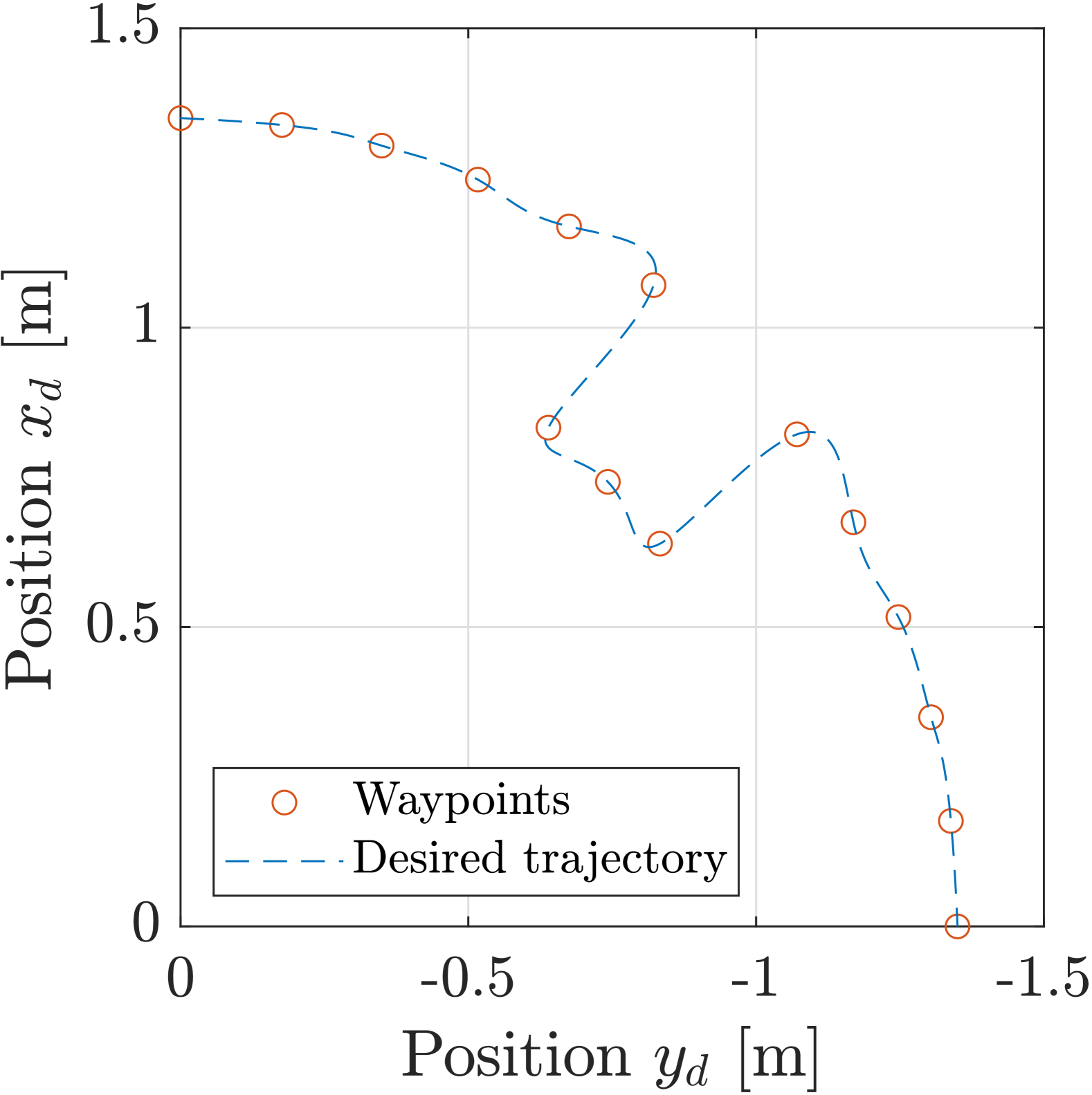
(a) Reference trajectory ($xy$-plot)

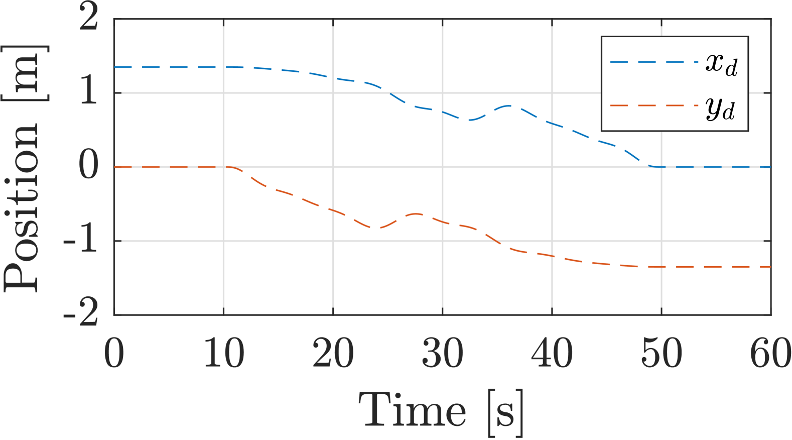
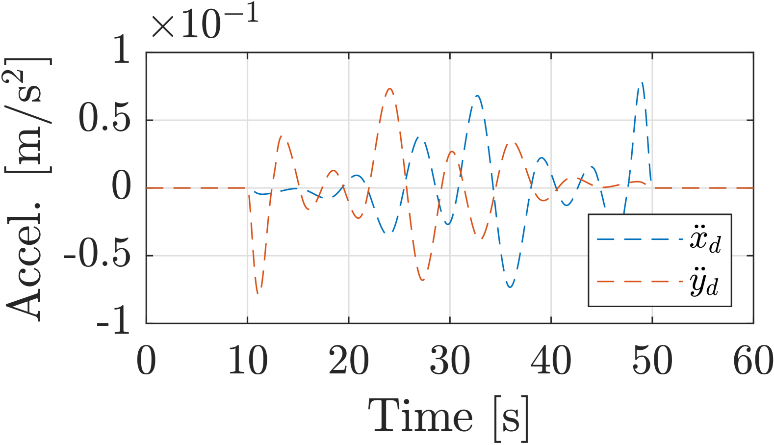
(b) Reference trajectory time history

Figure 1: Reference trajectory that was used in simulations for comparison of the Cartesian and angular controllers

The angular controller used the exponentially stabilizing damping controller presented in [34] for the crane load combined with a tracking controller [33] for the suspension point. The angular damping controller was tuned according to [34] with the undamped natural frequency ${\omega_{d}^{2}=k_{p,d}+\omega_{0}^{2}}$ and damping ratio ${\zeta_{d}=k_{d,d}/2\omega_{d}}$. The suspension point tracking controller was then tuned according to [33], selecting ${\omega_{t}=\omega_{d}/5}$ and ${\zeta_{t}\in[0.7,1]}$ to get the controller gains ${k_{p,t}=\omega_{t}^{2}}$ and ${k_{d,t}=2\zeta_{t}\omega_{t}}$. The controller parameters are given in Table 3 and below Table 4.

Table 3: Angular damping controller parameters

Parameter	Symbol	Value	Unit
Undamped natural frequency	$\omega_{d}$	$2.796$	$\mathrm{rad}\text{\,}{\mathrm{s}}^{-2}$
Relative damping	$\zeta_{d}$	$0.2$	-
Proportional gain	$k_{p,d}$	$0$	-
Derivative gain	$k_{d,d}$	$1.118$	-

Table 4: Suspension point tracking controller parameters

Parameter	Symbol	Value	Unit
Undamped natural frequency	$\omega_{t}$	$0.559$	$\mathrm{rad}\text{\,}{\mathrm{s}}^{-2}$
Relative damping	$\zeta_{t}$	$1$	-
Proportional gain	$k_{p,t}$	$0.313$	-
Derivative gain	$k_{d,t}$	$1.118$	-

The simulations demonstrated that tracking performance was significantly improved when the Cartesian controller was used compared to the angular controller. This was most evident during obstacle avoidance phase in the middle of the trajectory, where the angular controller gave significant overshoot, while the Cartesian controller tracked the trajectory accurately. The tracking performance is shown in Figures 2 and 3.

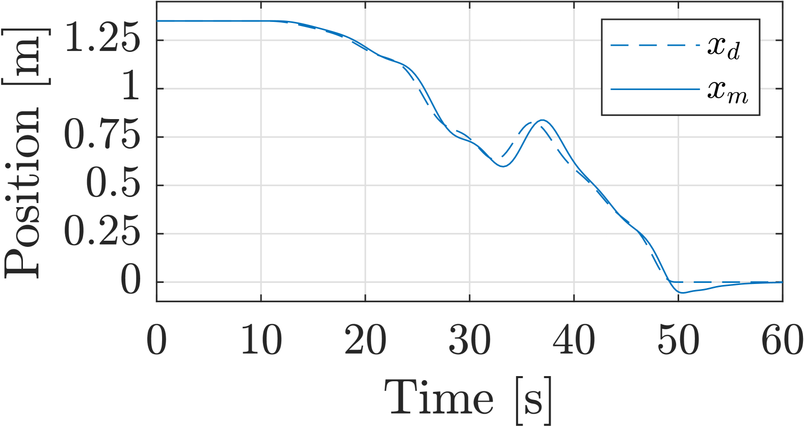
(a) Mass position $x_{m}$ and $x_{d}$

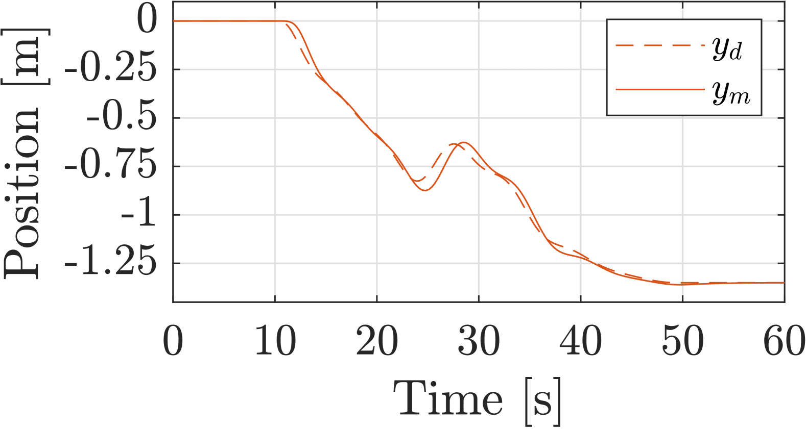
(b) Mass position $y_{m}$ and $y_{d}$

Figure 2: Angular controller tracking performance

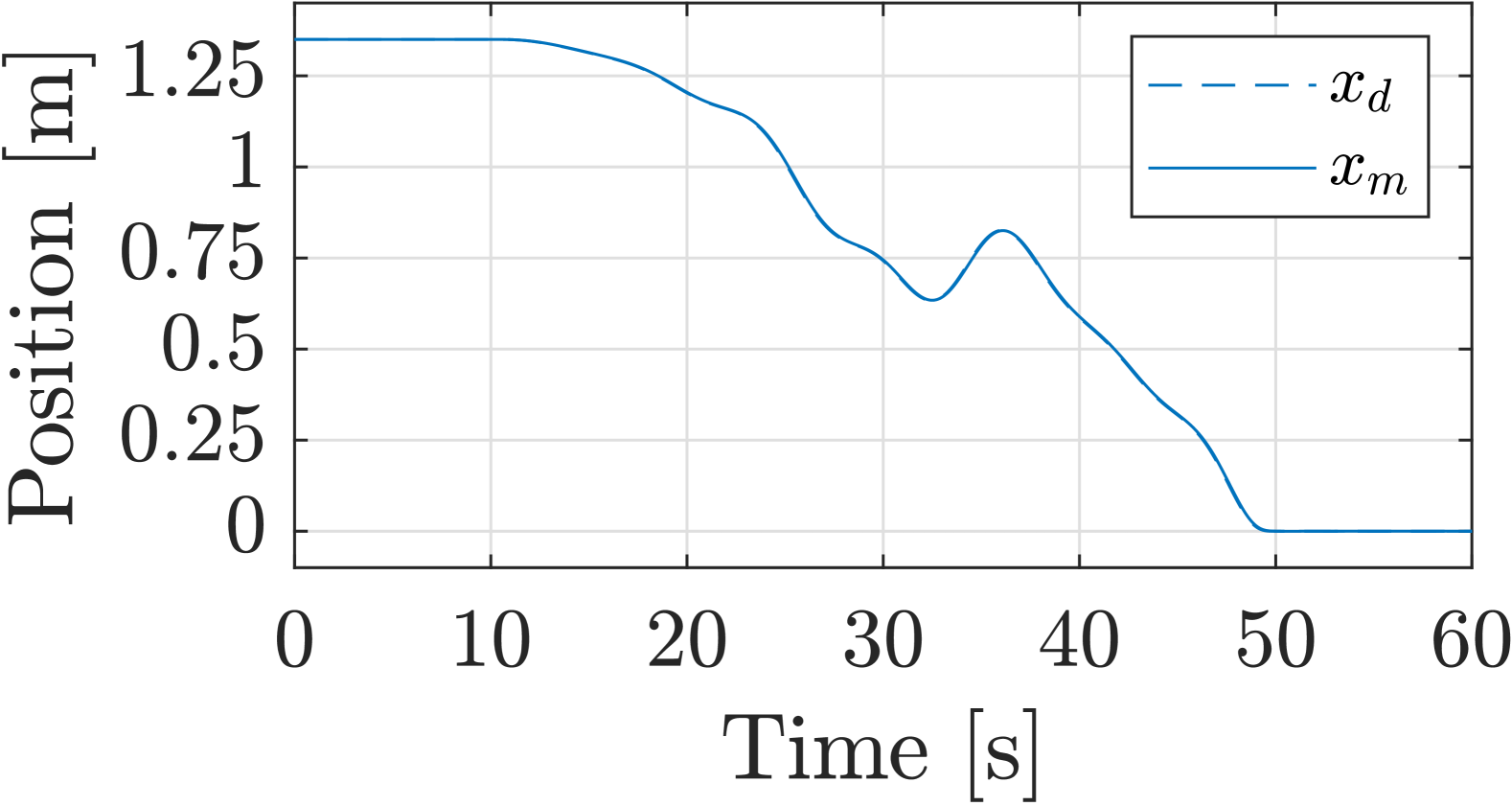
(a) Mass position $x_{m}$ and $x_{d}$

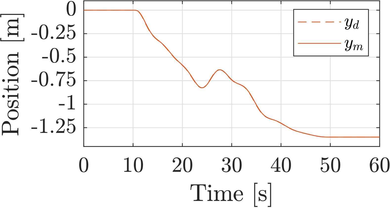
(b) Mass position $y_{m}$ and $y_{d}$

Figure 3: Cartesian controller tracking performance

The improvement in tracking performance was not a consequence of a less efficient actuation of the suspension point. The comparison showed that the velocity and acceleration of the suspension point were comparable between the angular and Cartesian controllers. This is shown in Figures 4 and 5 below, where the velocity and acceleration of the suspension point are compared using the angular and Cartesian controllers.

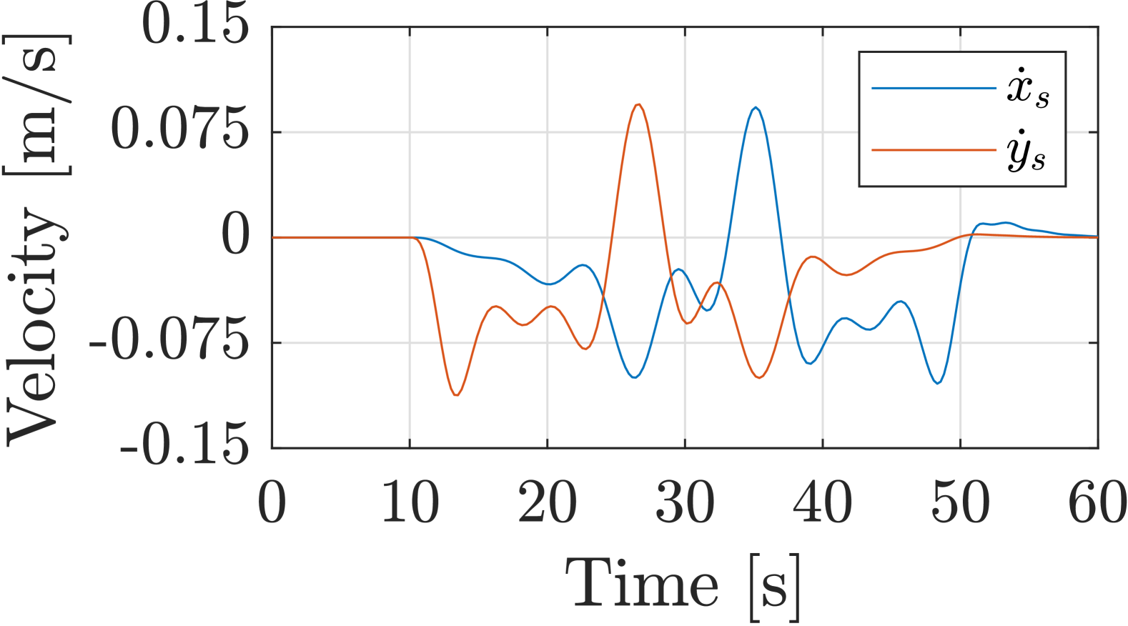
(a) Velocity ${\dot{x}_{s}}$ and ${\dot{y}_{s}}$

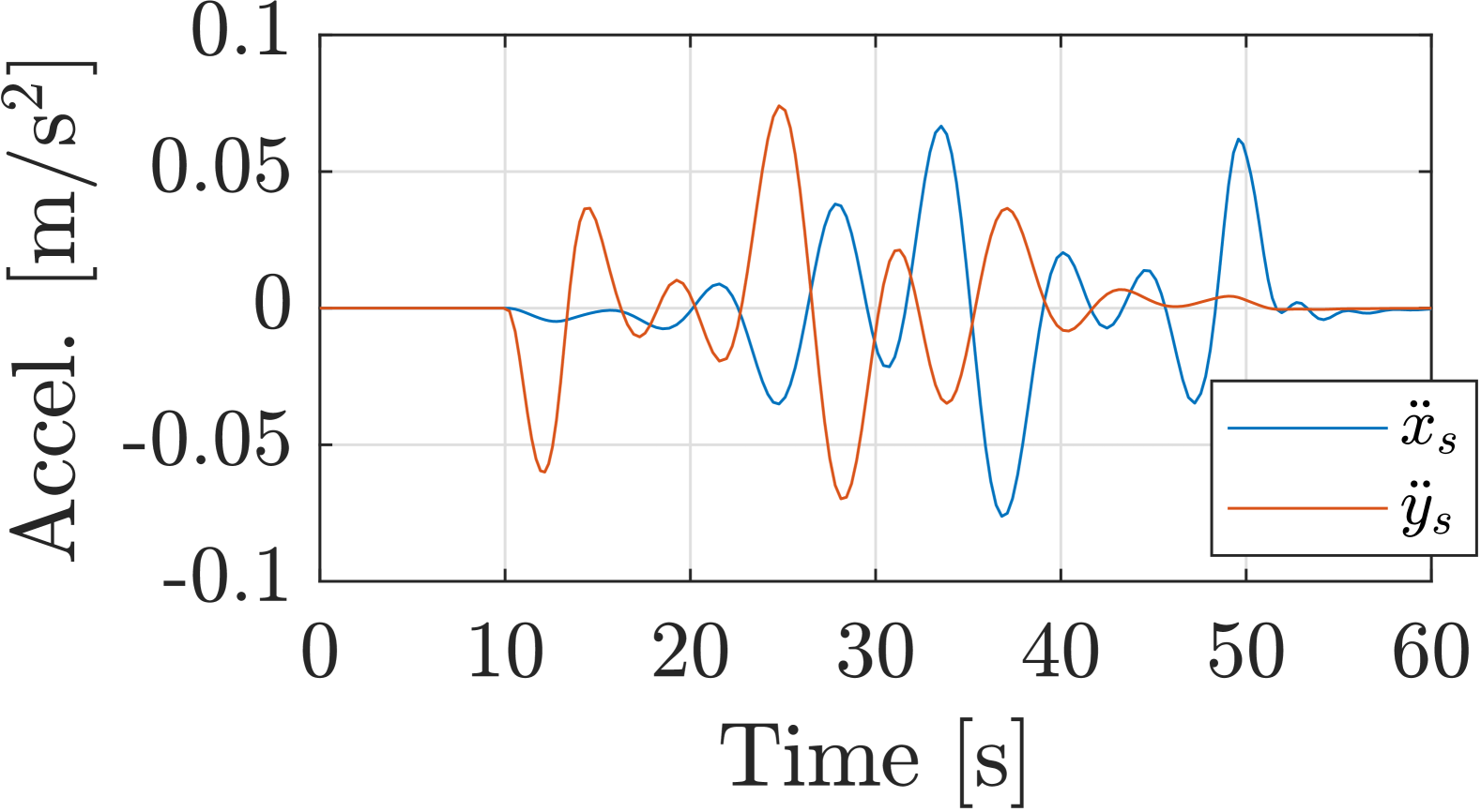
(b) Acceleration ${\ddot{x}_{s}}$ and ${\ddot{y}_{s}}$

Figure 4: Suspension point velocity and acceleration for the angular controller

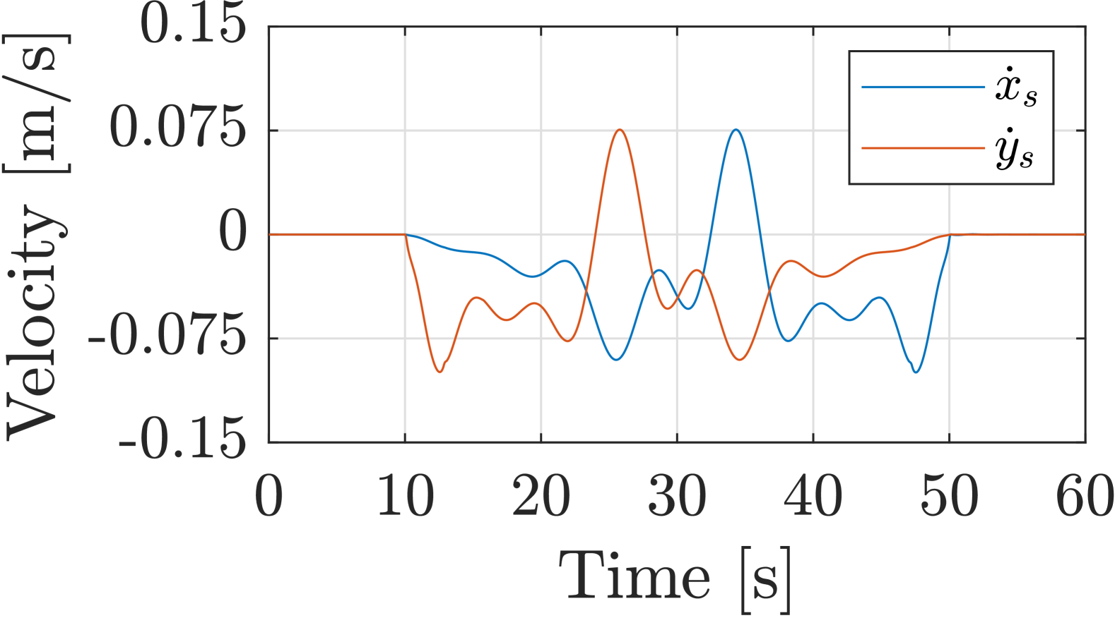
(a) Velocity ${\dot{x}_{s}}$ and ${\dot{y}_{s}}$

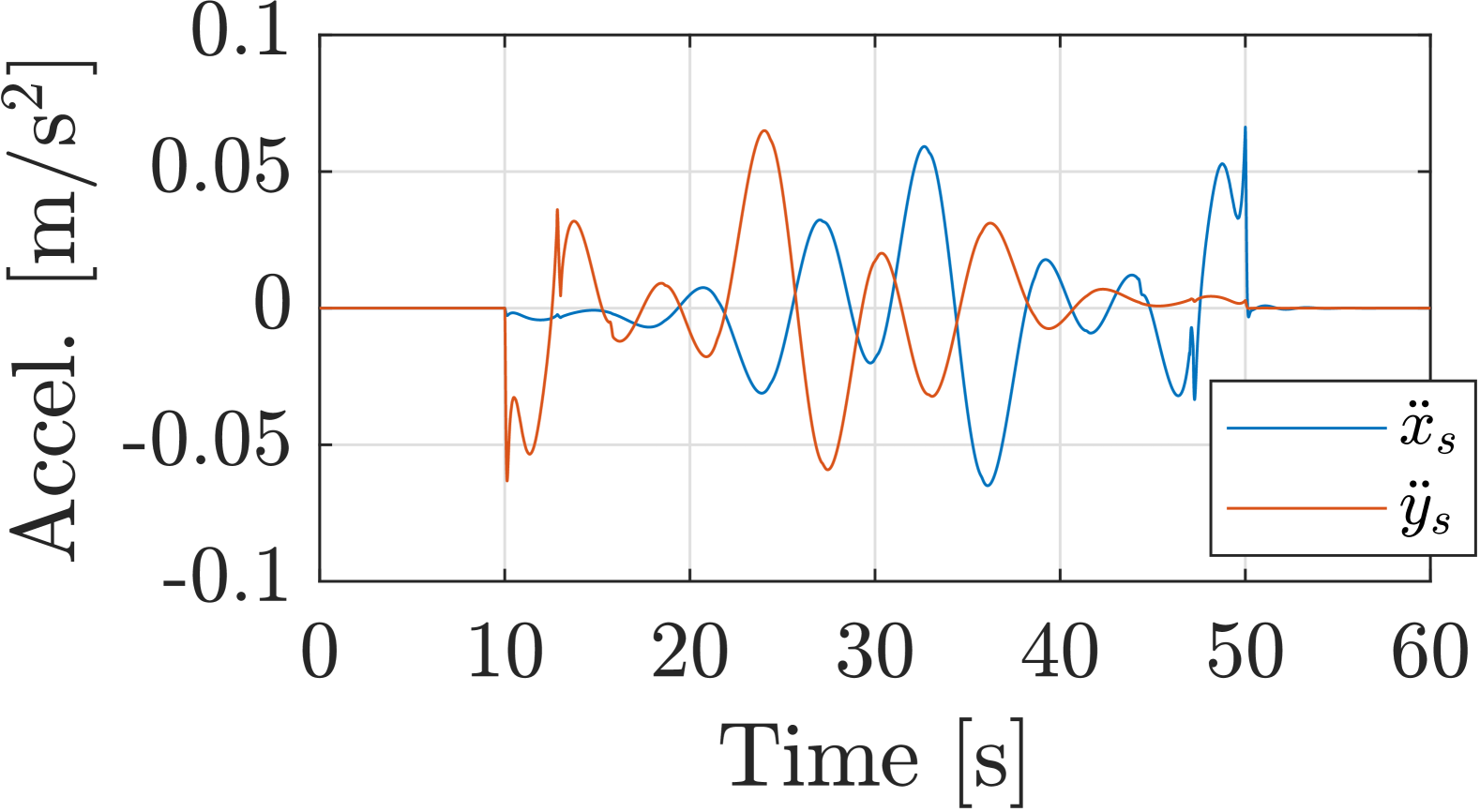
(b) Acceleration ${\ddot{x}_{s}}$ and ${\ddot{y}_{s}}$

Figure 5: Suspension point velocity and acceleration for the Cartesian controller

The tracking error for the mass point was significantly smaller for the Cartesian controller than for the angular controller, which is seen from Figures 6 and 7 and Table 9.

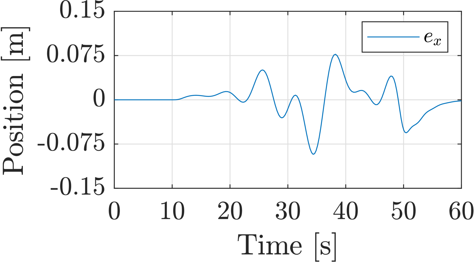
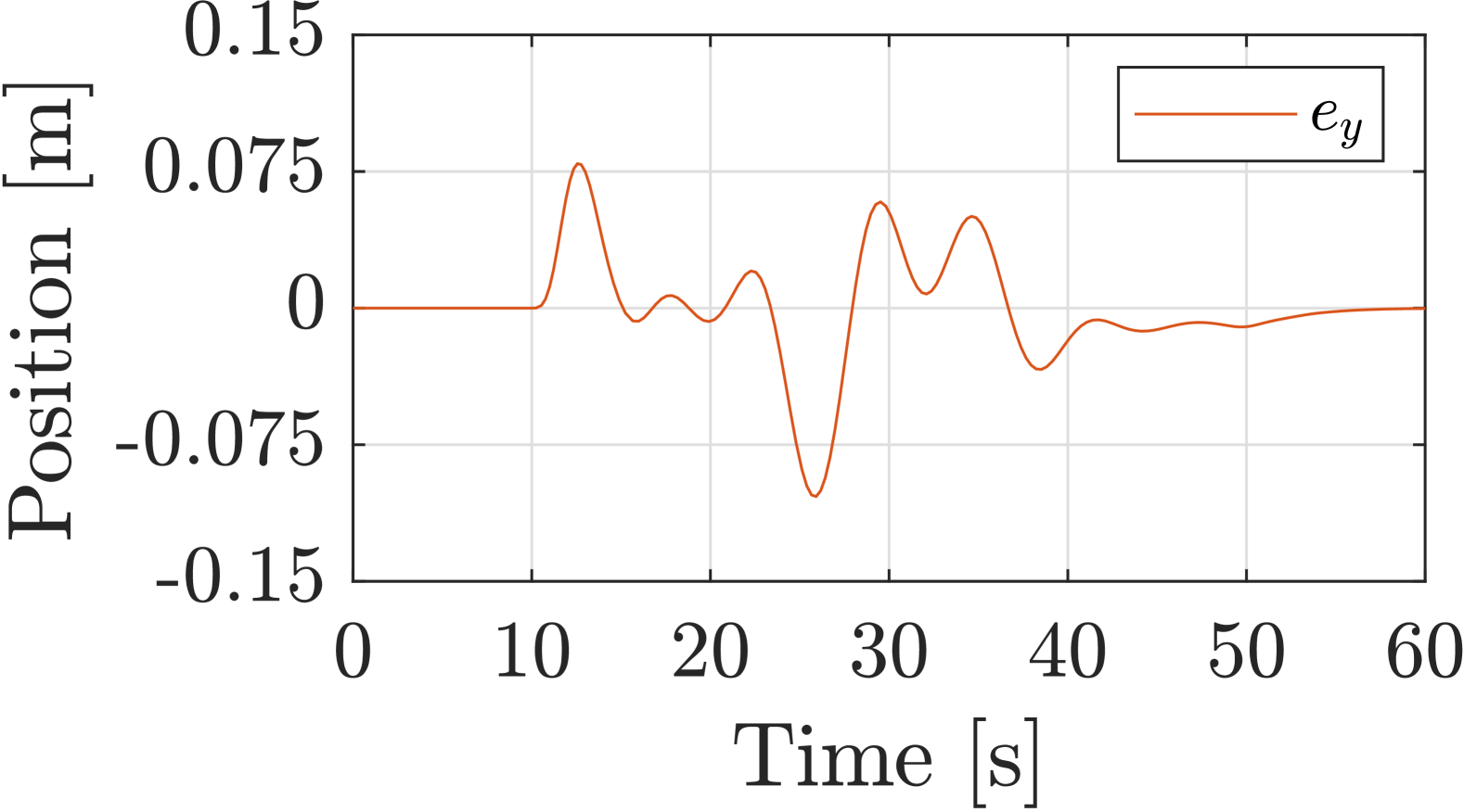
Figure 6: Position control error ${e_{x}}$ and ${e_{y}}$ for angular controller

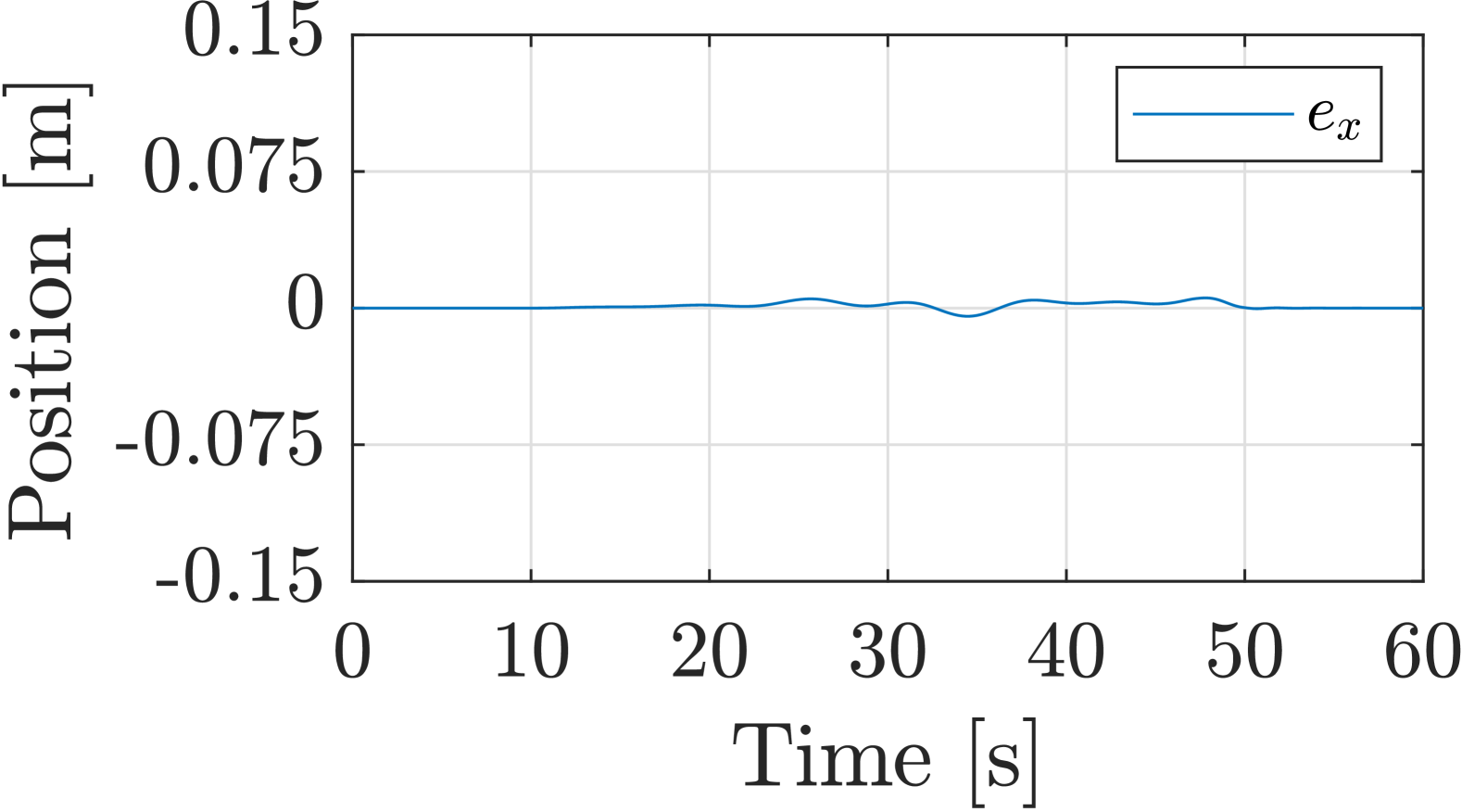
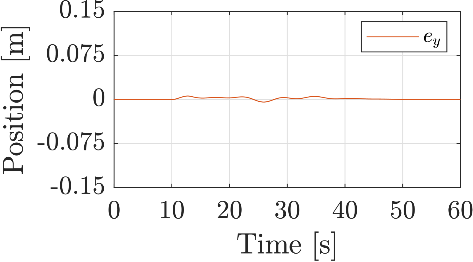
Figure 7: Position control error ${e_{x}}$ and ${e_{y}}$ for Cartesian controller

Table 5: Tracking error metrics - Angular and Cartesian

Metric	Angular	Cartesian	Improvement [%]
MSE	$2.04\cdot 10^{-3}$	$1.35\cdot 10^{-5}$	$99.34$
MAE	$3.39\cdot 10^{-2}$	$3.20\cdot 10^{-3}$	$90.57$

5.2 Simulations and experiments with the nonparametric adaptive controller

The nonparametric adaptive controller was tested in simulations and experiments and compared to the non-adaptive Cartesian tracking controller. The same reference trajectory of ${T=$40\text{\,}\mathrm{s}$}$ duration was used as in the simulation study of the previous section, but in this case the time history was different, and there was no obstacle in the middle of the trajectory. The reference trajectory started with zero velocity at ${x_{0}=$1.35\text{\,}\mathrm{m}$}$, ${y_{0}=$0\text{\,}\mathrm{m}$}$, and ended with zero velocity at ${x_{T}=$0\text{\,}\mathrm{m}$}$, ${y_{T}=$-1.35\text{\,}\mathrm{m}$}$ as shown in the $xy$-plot of Figure 8(a). A smooth sinusoidal acceleration profile was used to limit the jerk of the reference trajectory (Figure 8(b)). A $10\text{\,}\mathrm{s}$ buffer with zero velocity was added before the start and after the end of the reference trajectory.

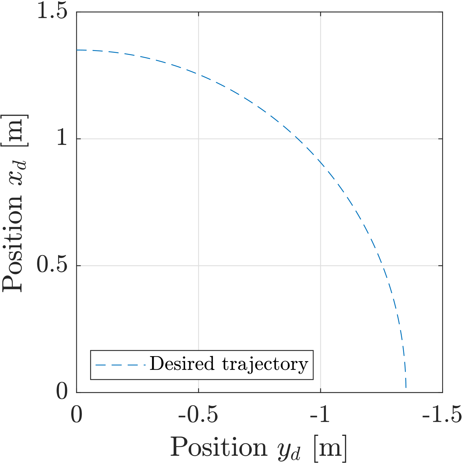
(a) Reference trajectory ($xy$-plot)

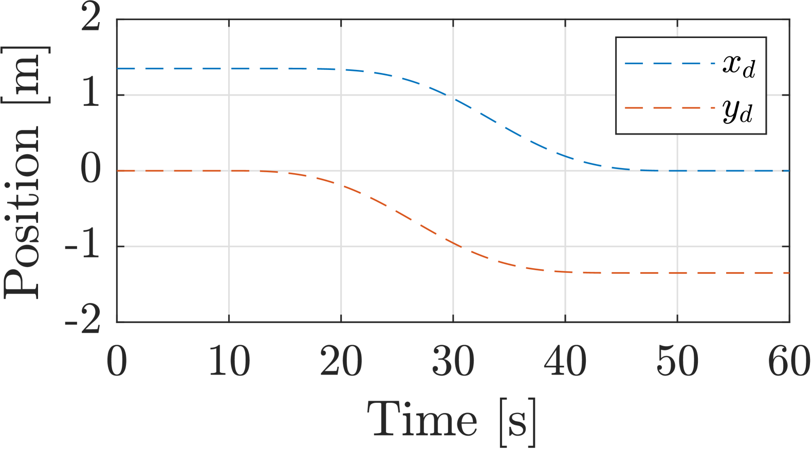
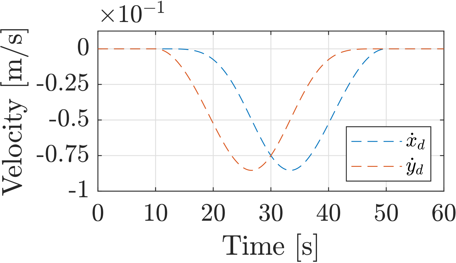
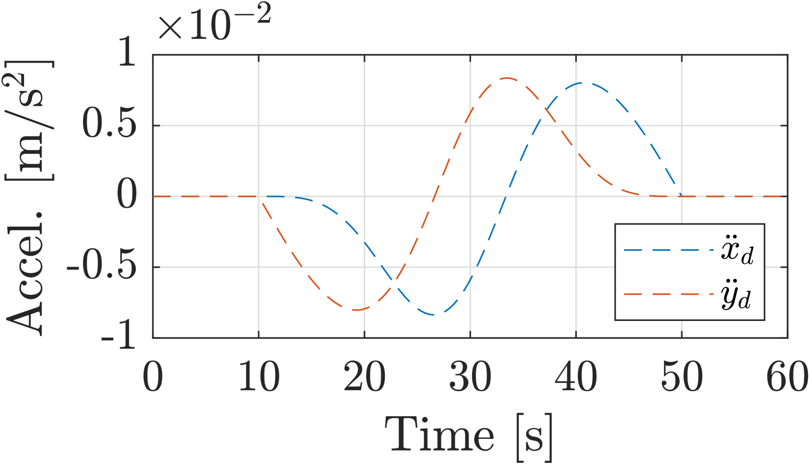
(b) Reference trajectory time histories

Figure 8: Reference trajectory for the adaptive control simulations and experiments

The main disturbance to be compensated for by the adaptive controller was due to a sinusoidal motion of the base of the crane, which was similar to the wave-induced motion of a crane base on a ship deck. This sinusoidal motion was along the $y$-axis of the world frame $n$, with a frequency equal to the natural frequency of the pendulum ${\omega_{0}=$2.796\text{\,}\mathrm{rad}\text{\,}{\mathrm{s}}^{-2}$}$ and an amplitude of ${a=$0.5\text{\,}\mathrm{m}$}$.

5.2.1 Simulation study

The crane with the nonparametric adaptive controller was simulated in Simulink. The parameters of the nonparametric adaptive controller used in the simulation are given in Table 6.

Table 6: Nonparametric adaptive controller parameters - Simulation

Parameter	Symbol	Value	Unit
Number of features	$d$	$100$	-
Kernel width	$\sigma$	$1.5$	-
Learning rate	$\gamma$	$9$	-
Lyapunov constant	$c$	$0.5$	-

The simulation results showed that the nonparametric adaptive controller gave a significant improvement in tracking performance compared to the Cartesian tracking controller. The effect of the sinusoidal motion of the base was significantly reduced, which improved the tracking performance of the crane load in the $y$-direction. Furthermore, the nonparametric adaptive controller also improved the tracking accuracy in the $x$-direction. Figures 9 and 10 show the simulated system without adaption and with adaption enabled, respectively.

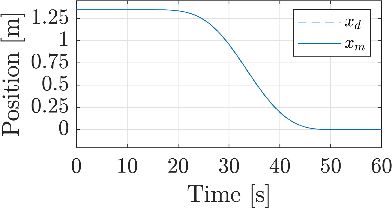
(a) Mass position $x_{m}$ and $x_{d}$

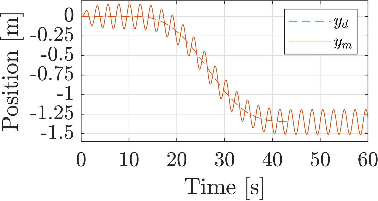
(b) Mass position $y_{m}$ and $y_{d}$

Figure 9: Simulation tracking results without adaption

(a) Mass position $x_{m}$ and $x_{d}$

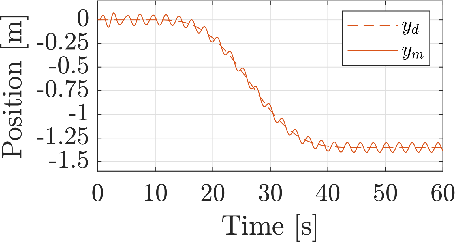
(b) Mass position $y_{m}$ and $y_{d}$

Figure 10: Simulation tracking results with adaption

The reduction in position tracking error is illustrated in Figures 11 and 12, where the position error in the $x$- and $y$-directions are shown for the non-adaptive and adaptive case. The improvement is quantified in Table 7.

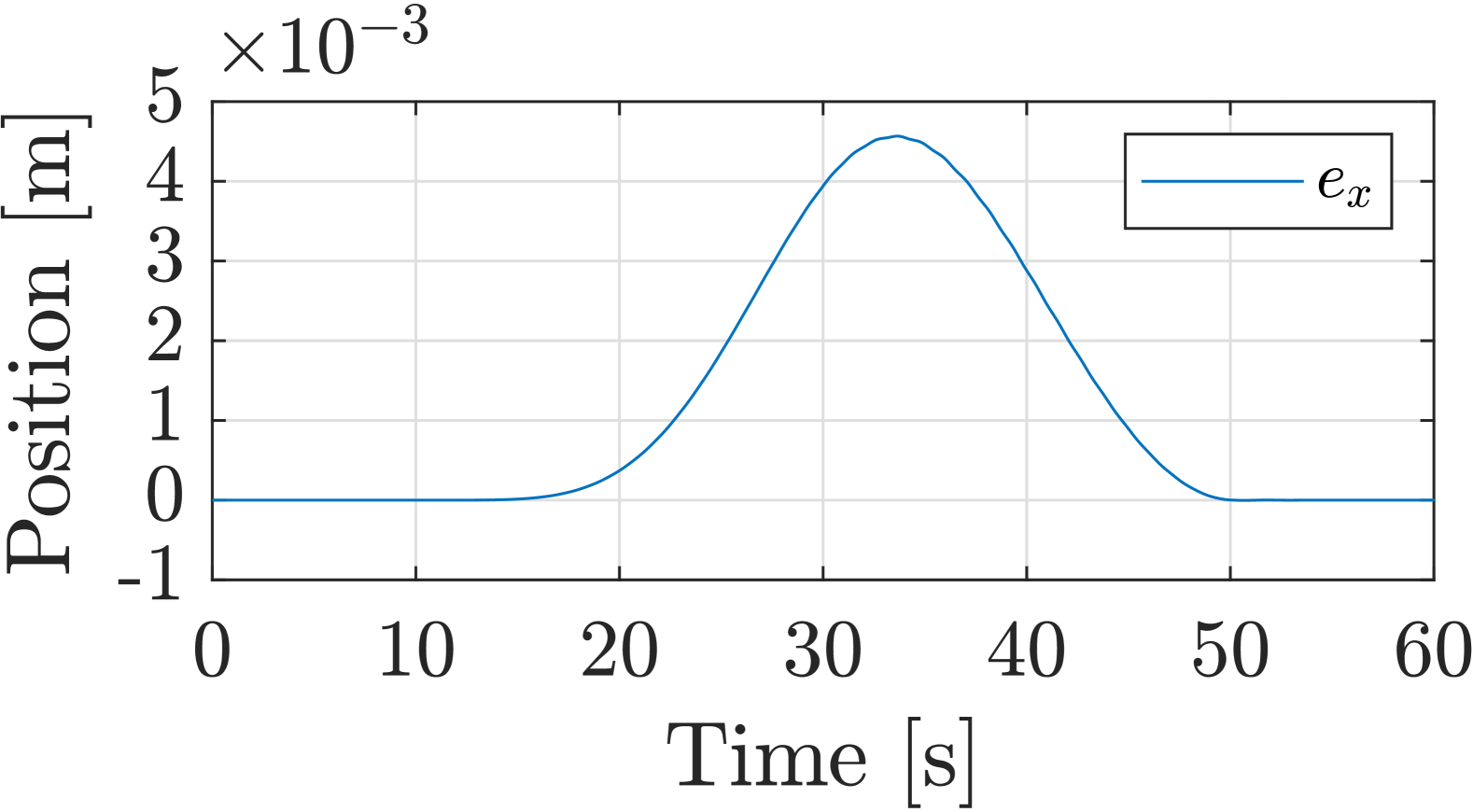
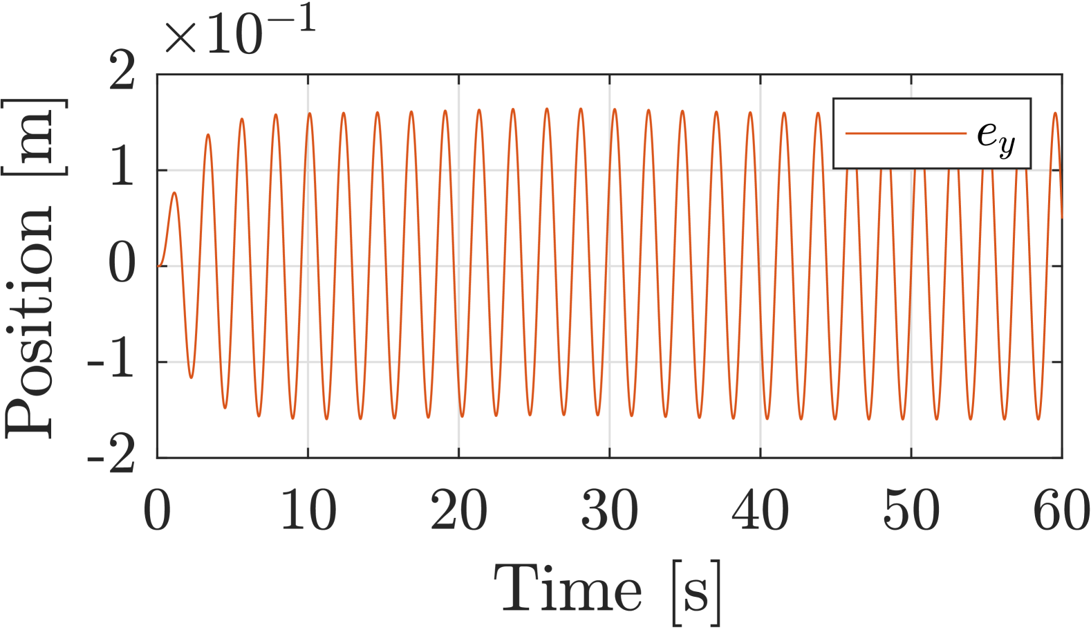
Figure 11: Simulation study error position without adaption

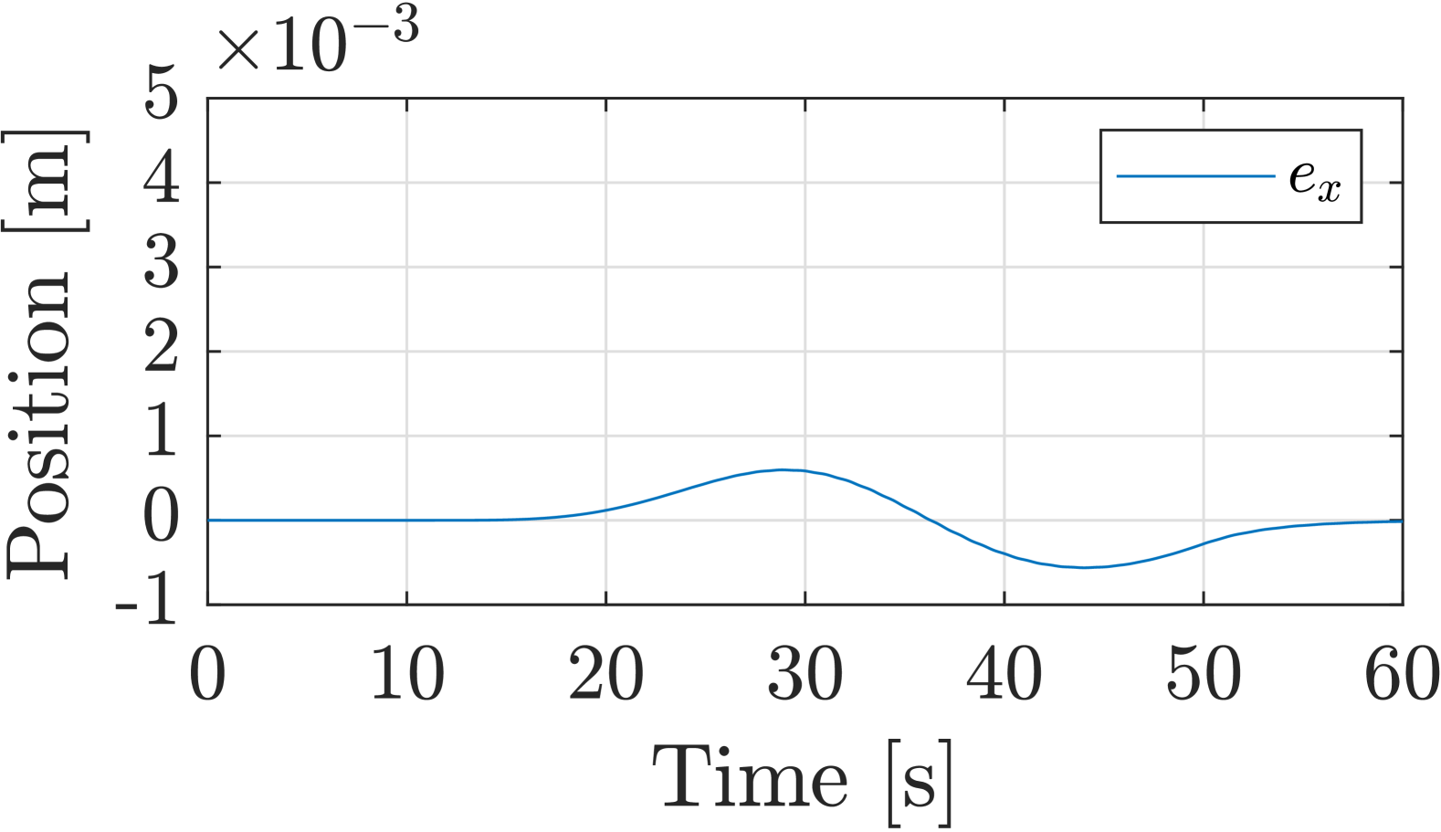
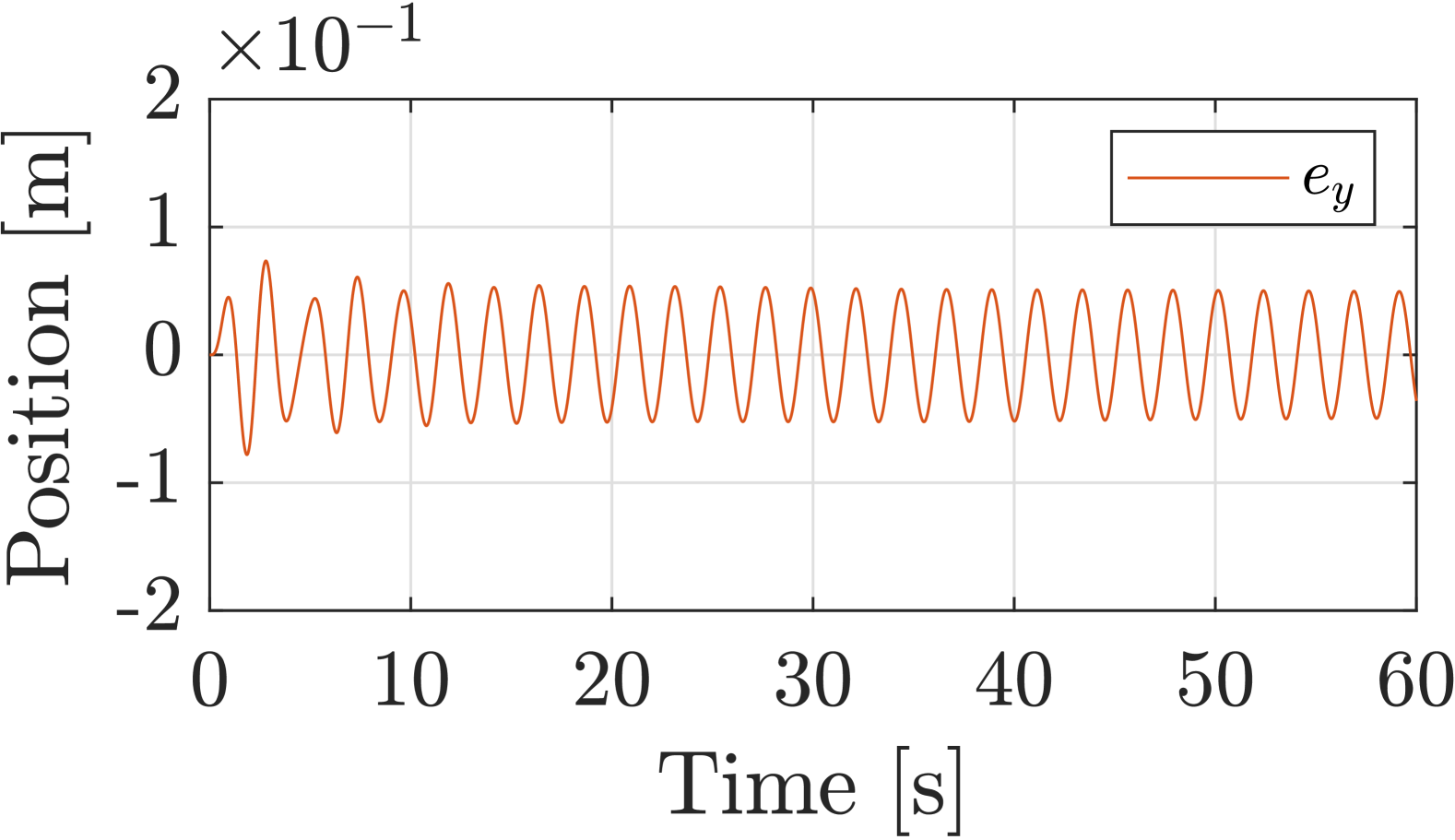
Figure 12: Simulation study error position with adaption

Table 7: Simulation - Tracking error metrics

Metric	W/o learn.	With learn.	Improvement [%]
MSE	$1.14\cdot 10^{-2}$	$1.50\cdot 10^{-3}$	$86.83$
MAE	$9.47\cdot 10^{-2}$	$3.52\cdot 10^{-2}$	$62.79$

A closer inspection of the results further explains the improved tracking performance. The adaptive controller learns to counteract both the tracking error in the $x$-direction and the sinusoidal disturbance in the $y$-direction. This is shown in Figure 13.

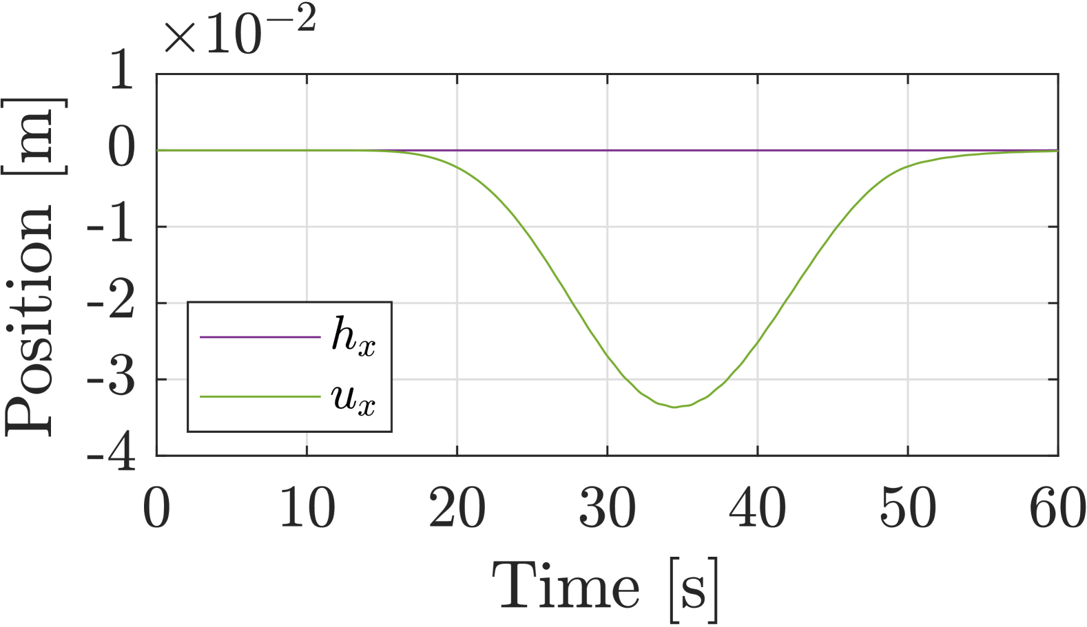
(a) Disturbance $h_{x}$ and adaptive input $u_{x}$

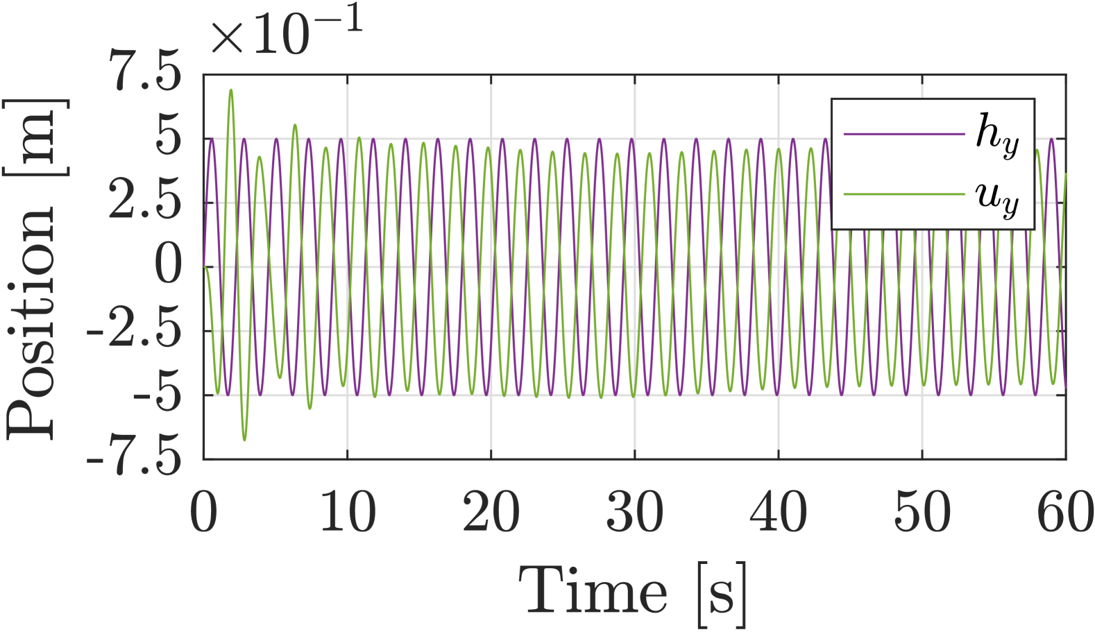
(b) Disturbance $h_{y}$ and adaptive input $u_{y}$

Figure 13: Simulation study disturbance and adaptive input with learning enabled

5.2.2 Experimental validation

The experiments were performed with a KUKA KR120 industrial robot which replaced the crane, using KUKA RobotSensorInterface to control the robot end effector (suspension point) in world frame coordinates and to read the position and velocity of the suspension point. For state feedback for the crane payload, a vision system using an Intel RealSense d435i camera was used with OpenCV to track the position of a ChArUco board attached to the crane payload. The position measurements of the payload were filtered using a low-pass filter, and the linear velocities of the payload were estimated using backward difference.

The software was implemented in Python and was separated into a slow and fast process using multiprocessing. The slow process included the vision system, the tracking controller, and the nonparametric adaptive controller, and ran at $30\text{\,}\mathrm{Hz}$, limited by the Intel RealSense d435i camera frame rate. The control input from the slow process was sent to the fast process running at $250\text{\,}\mathrm{Hz}$ as required by the communication interface with the KR120 robot, sending position updates using KUKA RSI Ethernet.

Due to the noise level in the vision system, deadzones were implemented and a more conservative tuning of the nonparametric adaptive controller was used in the experiments. The parameters of the nonparametric adaptive controller used in the real experiment are given in Table 8.

Table 8: Nonparametric adaptive controller parameters - Experimental validation

Parameter	Symbol	Value	Unit
Number of features	$d$	$1000$	-
Kernel width	$\sigma$	$0.5$	-
Learning rate	$\gamma$	$7$	-
Lyapunov constant	$c$	$0.5$	-
Deadzone cutoff constant	$\delta$	$0.007$	-
Deadzone smoothing constant	$\mu$	$0.002$	-

The experiments showed a significant improvement in tracking performance in the $y$-direction but a negligible improvement in the $x$-direction. The nonparametric adaptive controller was able to learn and cancel much of the disturbance, leading to a significant improvement in tracking performance. Figures 14 and 15 show the system tracking performance without and with learning enabled, respectivly.

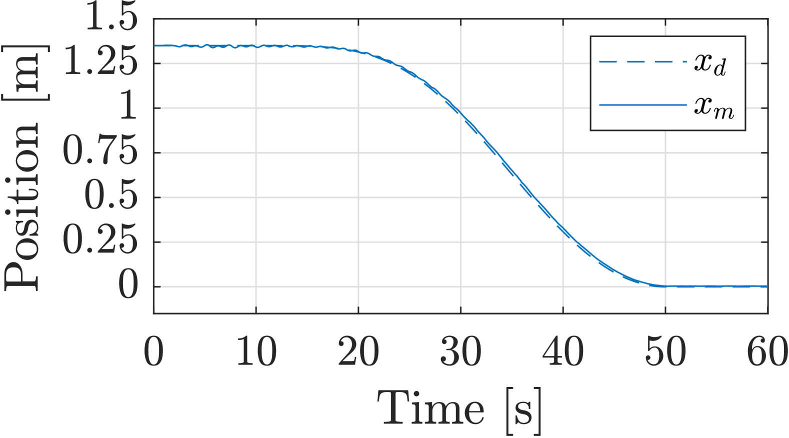
(a) Mass position $x_{m}$ and $x_{d}$

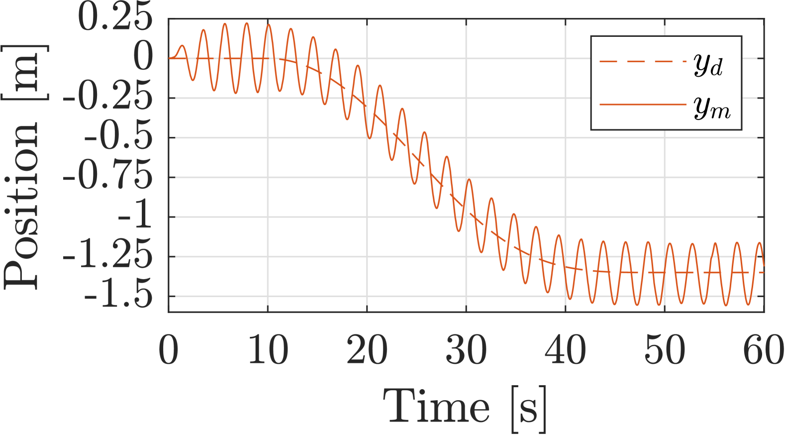
(b) Mass position $y_{m}$ and $y_{d}$

Figure 14: Experimental validation tracking results without learning

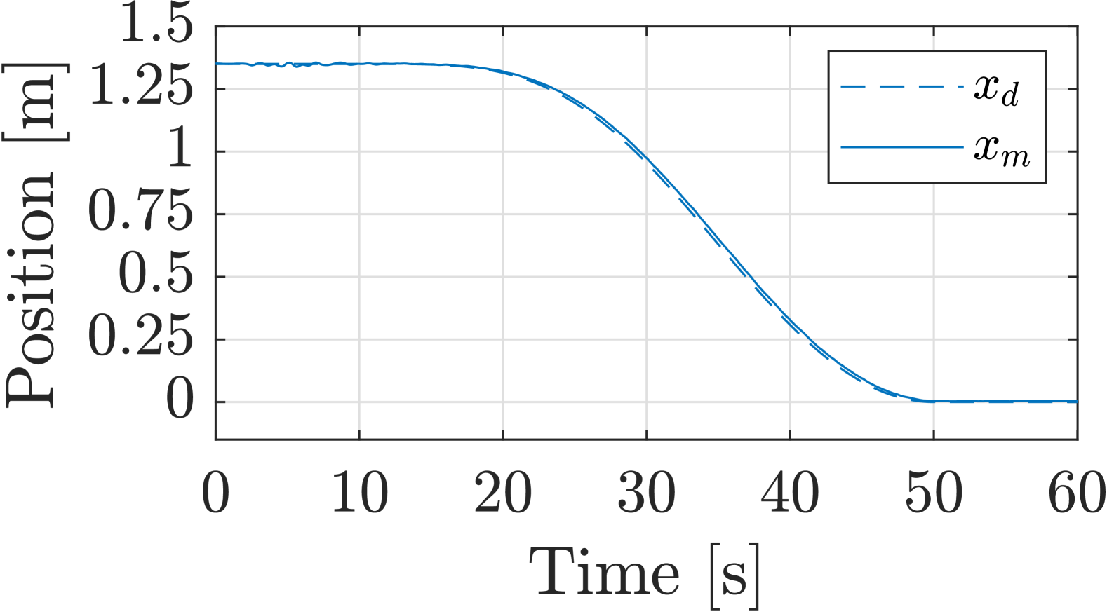
(a) Mass position $x_{m}$ and $x_{d}$

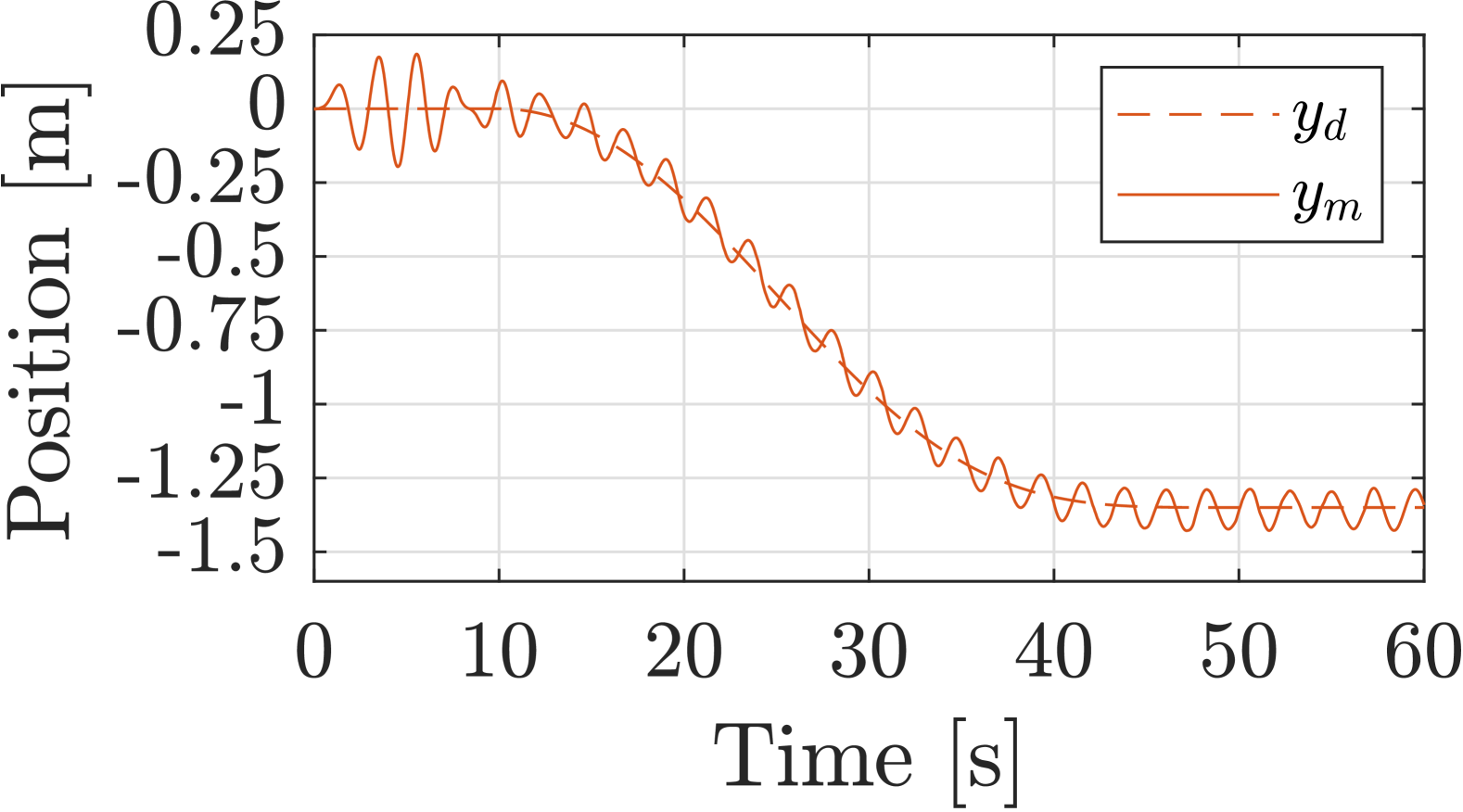
(b) Mass position $y_{m}$ and $y_{d}$

Figure 15: Experimental validation tracking results with learning

As seen from the position error ${e_{y}}$ shown in Figure 16, the improvement is significant, as the nonparametric adaptive controller learns and cancels the disturbance. The improvement is quantified in Table 9, and the learned control input from the nonparametric adaptive controller compared to the disturbance in the $y$-direction is shown in Figure 17.

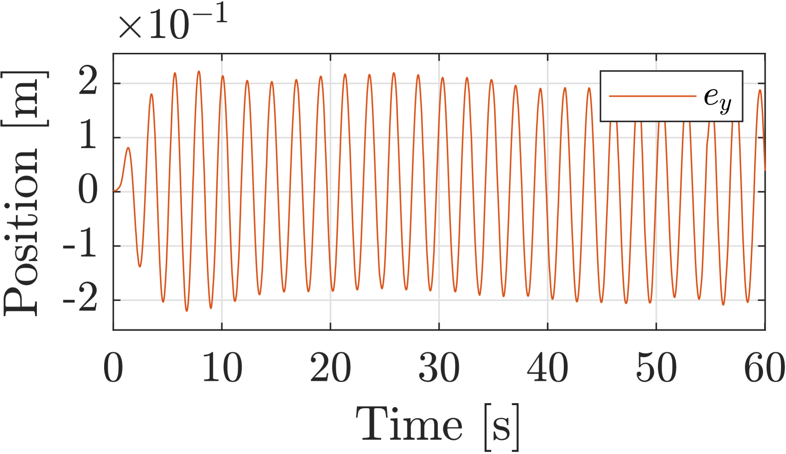
(a) Position error ${e_{y}}$ without learning

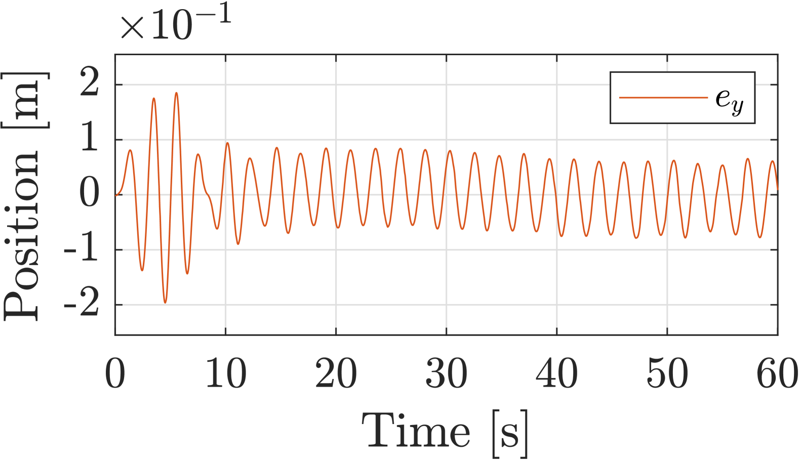
(b) Position error ${e_{y}}$ with learning

Figure 16: Experimental validation error position without and with learning compared

Table 9: Tracking error metrics - Experimental validation

Metric	W/o learn.	With learn.	Improvement [%]
MSE	$1.93\cdot 10^{-2}$	$3.66\cdot 10^{-3}$	$81.05$
MAE	$1.24\cdot 10^{-1}$	$5.16\cdot 10^{-2}$	$58.47$

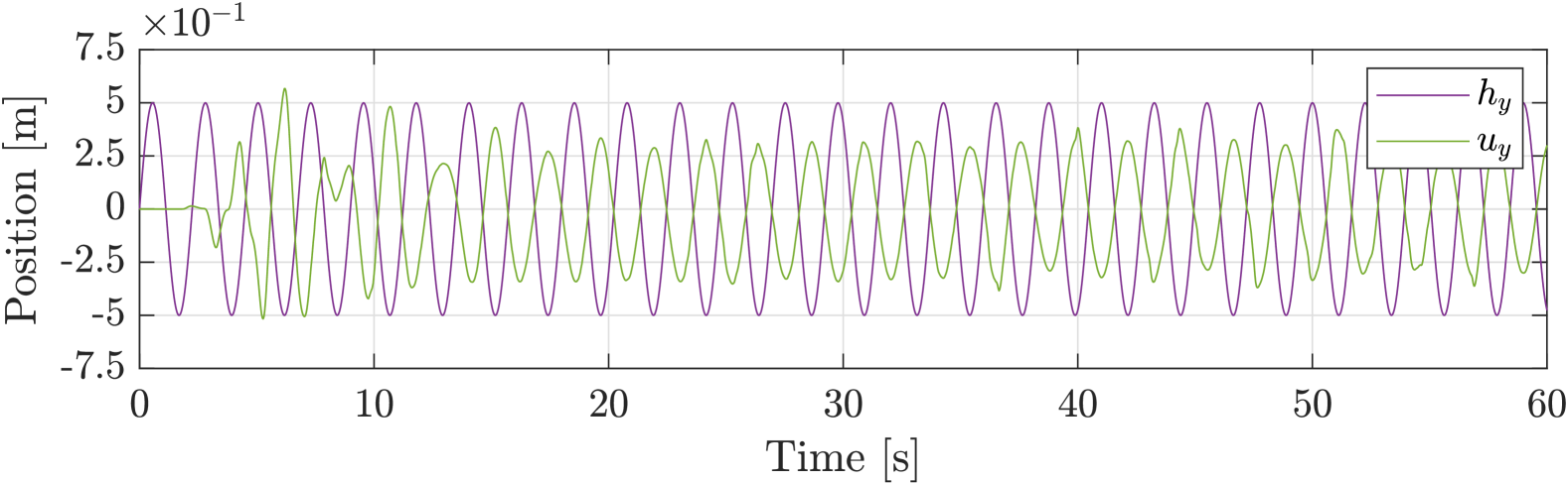
Figure 17: Experimental validation disturbance and adaptive input with learning enabled

6 Conclusion

A novel control algorithm has been presented for the automatic control of an offshore crane. The control algorithm uses a novel Cartesian model of a crane to design a Lyapunov-based tracking controller. The controller stabilizes the crane payload and tracks the reference trajectory, eliminating the need for a cascade of separate stabilizing and tracking controllers. Formal proofs have been presented which show that the proposed controller can track a reference trajectory with exponential stability. The Cartesian formulation allows the use of the novel nonparametric adaptive controller for disturbance rejection, such as wave disturbances, which is of high interest for an offshore crane.

Simulations show that a controller is more efficient and accurate for trajectory tracking than an angular formulation. The tracking performance, as measured by the MSE of the tracking error, is improved by $99.34\%$ with a comparable velocity and acceleration of the suspension point. The nonparametric adaptive controller has been tested in simulation and experiments on an industrial robot. The tracking error MSE improved by $86.83\%$ in the simulation and $81.05\%$ in the experiments. This shows that the proposed controller significantly improves tracking performance when subject to disturbances.

Appendix A Feature map for the Gaussian kernel

A feature map for the Gaussian kernel

$$k({\bm{x}},{\bm{z}})=\exp\left(-\frac{({\bm{x}}-{\bm{z}})^{\rm T}({\bm{x}}-{\bm{z}})}{2\sigma^{2}}\right)$$ (105)

is derived in [24] from

$$k({\bm{x}},{\bm{z}}) =\exp\left(-\frac{{\bm{x}}^{\rm T}{\bm{x}}}{2\sigma^{2}}\right)\exp\left(-\frac{{\bm{z}}^{\rm T}{\bm{z}}}{2\sigma^{2}}\right)\exp\left(\frac{{\bm{x}}^{\rm T}{\bm{z}}}{\sigma^{2}}\right)$$

$$=\exp\left(-\frac{{\bm{x}}^{\rm T}{\bm{x}}}{2\sigma^{2}}\right)\exp\left(-\frac{{\bm{z}}^{\rm T}{\bm{z}}}{2\sigma^{2}}\right)\sum_{k=0}^{\infty}\frac{({\bm{x}}^{\rm T}{\bm{z}})^{k}}{k!}$$ (106)

The term $({\bm{x}}^{\rm T}{\bm{z}})^{k}$ gives

$$({\bm{x}}^{\rm T}{\bm{z}})^{k} =(x_{1}z_{1}+\ldots+x_{n}z_{n})^{k}$$

$$=\sum_{k_{1}+\ldots+k_{n}=k}\frac{k!}{k_{1}!\ldots k_{n}!}(x_{1}z_{1})^{k_{1}}\ldots(x_{n}z_{n})^{k_{n}}$$

$$=\sum_{k_{1}+\ldots+k_{n}=k}\sqrt{\frac{k!}{k_{1}!\ldots k_{n}!}}x_{1}^{k_{1}}\ldots x_{n}^{k_{n}}\sqrt{\frac{k!}{k_{1}!\ldots k_{n}!}}z_{1}^{k_{1}}\ldots z_{n}^{k_{n}}$$ (107)

where the second equality is due to the binomial theorem. The kernel can therefore be written as

$$k({\bm{x}},{\bm{z}}) =\sum_{k=0}^{\infty}\left(\sum_{k_{1}+\ldots+k_{n}=k}\frac{\exp\left(-\frac{{\bm{x}}^{\rm T}{\bm{x}}}{2\sigma^{2}}\right)}{\sqrt{k_{1}!\ldots k_{n}!}}x_{1}^{k_{1}}\ldots x_{n}^{k_{n}}\frac{\exp\left(-\frac{{\bm{z}}^{\rm T}{\bm{z}}}{2\sigma^{2}}\right)}{\sqrt{k_{1}!\ldots k_{n}!}}z_{1}^{k_{1}}\ldots z_{n}^{k_{n}}\right)$$ (108)

Define the infinite-dimensional feature map ${\bm{\phi}}=[\phi_{0},\phi_{1},\phi_{2}\ldots]^{\rm T}$ by the components

$$\phi_{k}({\bm{x}})=\frac{\exp\left(-\frac{{\bm{x}}^{\rm T}{\bm{x}}}{2\sigma^{2}}\right)}{\sqrt{k_{1}!\ldots k_{n}!}}x_{1}^{k_{1}}\ldots x_{n}^{k_{n}},\quad k=0,1,2\ldots$$ (109)

where $k_{1}+\ldots+k_{n}=k$ and $k_{1},\ldots k_{n}\geq 0$. This is a feature map for the Gaussian kernel since

$$k({\bm{x}},{\bm{z}})=\sum_{k=0}^{\infty}\phi_{k}({\bm{x}})^{\rm T}\phi_{k}({\bm{z}})={\bm{\phi}}({\bm{x}})^{\rm T}{\bm{\phi}}({\bm{z}})$$ (110)

Appendix B Crane model in Cartesian coordinates

B.1 Kane’s equations of motion for a spherical pendulum

The Cartesian model is derived from the dynamic model using angular coordinates [34] by introducing a change of coordinates. The inertial frame $n$ is defined with the $z$-axis pointing upwards. The body-fixed frame $b$ is defined with the $z$ axis along the crane wire. The rotation from frame $n$ to frame $b$ is given by the Euler angles $\phi_{x}$ about the $x$ axis of the $n$ frame followed by a rotation $\phi_{y}$ about the resulting $y$ axis. The rotation matrix is then ${\bm{R}}^{n}_{b}={\bm{R}}_{x}(\phi_{x}){\bm{R}}_{y}(\phi_{y})$. This gives

$${\bm{R}}^{n}_{b}=\left[\begin{array}[]{ccc}1&0&0\\ 0&c_{x}&-s_{x}\\ 0&s_{x}&c_{x}\end{array}\right]\left[\begin{array}[]{ccc}c_{y}&0&s_{y}\\ 0&1&0\\ -s_{y}&0&c_{y}\end{array}\right]=\left[\begin{array}[]{ccc}c_{y}&0&s_{y}\\ s_{x}s_{y}&c_{x}&-s_{x}c_{y}\\ -c_{x}s_{y}&s_{x}&c_{x}c_{y}\end{array}\right]$$ (111)

The position of the crane tip in the coordinates of $n$ is ${\bm{r}}_{0}^{n}$ and the position of the mass is

$${\bm{r}}^{n}={\bm{r}}_{0}^{n}+{\bm{R}}^{n}_{b}{\bm{r}}_{r}^{b}$$ (112)

where ${\bm{r}}_{r}^{b}=[0,0,-L]^{\rm T}$. The velocity is ${\bm{v}}^{n}=\dot{\bm{r}}^{n}$ and the acceleration is ${\bm{a}}^{n}=\ddot{\bm{r}}^{n}$. The coordinate expressions are

$${\bm{r}}^{n}=\left[\begin{array}[]{c}x\\ y\\ z\end{array}\right]=\left[\begin{array}[]{c}x_{0}-s_{y}L\\ y_{0}+s_{x}c_{y}L\\ z_{0}-c_{x}c_{y}L\end{array}\right]$$ (113)

and

$${\bm{v}}^{n}=\left[\begin{array}[]{c}\dot{x}_{0}-c_{y}\dot{\phi}_{y}L-s_{y}\dot{L}\\ \dot{y}_{0}+c_{x}c_{y}\dot{\phi}_{x}L-s_{x}s_{y}\dot{\phi}_{y}L+s_{x}c_{y}\dot{L}\\ \dot{z}_{0}+s_{x}c_{y}\dot{\phi}_{x}L+c_{x}s_{y}\dot{\phi}_{y}L-c_{x}c_{y}\dot{L}\end{array}\right]$$ (114)

The acceleration is then found by differentiation of the velocity components to be

$$\ddot{x} =\ddot{x}_{0}-c_{y}\ddot{\phi}_{y}L+s_{y}\dot{\phi}_{y}^{2}L-2c_{y}\dot{\phi}_{y}\dot{L}-s_{y}\ddot{L}$$ (115)

$$\ddot{y} =\ddot{y}_{0}-Ls_{x}c_{y}(\dot{\phi}_{x}^{2}+\dot{\phi}_{y}^{2})-2Lc_{x}s_{y}\dot{\phi}_{x}\dot{\phi}_{y}+Lc_{x}c_{y}\ddot{\phi}_{x}-Ls_{x}s_{y}\ddot{\phi}_{y}$$ (116)

$$\quad\quad-2\dot{L}(-c_{x}c_{y}\dot{\phi}_{x}+s_{x}s_{y}\dot{\phi}_{y})+\ddot{L}s_{x}c_{y}$$ (117)

$$\ddot{z} =\ddot{z}_{0}+Lc_{x}c_{y}(\dot{\phi}_{x}^{2}+\dot{\phi}_{y}^{2})-2Ls_{x}s_{y}\dot{\phi}_{x}\dot{\phi}_{y}+Ls_{x}c_{y}\ddot{\phi}_{x}+Lc_{x}s_{y}\ddot{\phi}_{y}$$ (118)

$$\quad\quad+2\dot{L}(s_{x}c_{y}\dot{\phi}_{x}+c_{x}s_{y}\dot{\phi}_{y})-\ddot{L}c_{x}c_{y}$$ (119)

The partial velocities with respect to the generalized speeds $(\dot{\phi}_{x},\dot{\phi}_{y})$, which are used in the development of Kane’s equation of motion, are found from (114) to be

$${\bm{v}}_{1} =\frac{\partial{\bm{v}}^{n}}{\partial\dot{\phi}_{x}}=\left[\begin{array}[]{c}0\\ Lc_{x}c_{y}\\ Ls_{x}c_{y}\end{array}\right]$$ (123)

$${\bm{v}}_{2} =\frac{\partial{\bm{v}}^{n}}{\partial\dot{\phi}_{y}}=\left[\begin{array}[]{c}-Lc_{y}\\ -Ls_{x}s_{y}\\ Lc_{x}s_{y}\end{array}\right]$$ (127)

Kane’s equations of motion are then found from

$${\bm{v}}_{1}^{\rm T}(-m{\bm{a}}^{n}+m{\bm{g}}^{n}+{\bm{F}}) =0$$ (128)

$${\bm{v}}_{2}^{\rm T}(-m{\bm{a}}^{n}+m{\bm{g}}^{n}+{\bm{F}}) =0$$ (129)

where ${\bm{F}}=[F_{x},F_{y},F_{z}]^{\rm T}$ is the external force acting on the load and ${\bm{g}}=[0,0,-g]^{\rm T}$ is the acceleration of gravity, where $g=$9.81\text{\,}\mathrm{m}\text{\,}{\mathrm{s}}^{-2}$$. After some simplifications, this gives

$$mLc_{y}\left(-c_{x}\ddot{y}_{0}-s_{x}\ddot{z}_{0}+2\dot{L}c_{y}\dot{\phi}_{x}+2Ls_{y}\dot{\phi}_{x}\dot{\phi}_{y}-Lc_{y}\ddot{\phi}_{x}\right)\quad$$

$$-Ls_{x}c_{y}mgL+Lc_{x}c_{y}F_{y}+Ls_{x}c_{y}F_{z} =0$$ (130)

$$mL\left(c_{y}\ddot{x}_{0}+\ddot{y}_{0}s_{x}s_{y}-\ddot{z}_{0}c_{x}s_{y}-Ls_{y}c_{y}\dot{\phi}_{x}^{2}-L\ddot{\phi}_{y}\right)\quad$$

$$-Lc_{x}s_{y}mg-Lc_{y}F_{x}-Ls_{x}s_{y}F_{y}+Lc_{x}s_{y}F_{z} =0$$ (131)

Division of the first equation by $mL^{2}c_{y}$ and the second by $mL^{2}$ gives

$$\ddot{\phi}_{x}c_{y}+\omega_{0}^{2}s_{x} =\frac{1}{L}\left(-\ddot{y}_{0}c_{x}-\ddot{z}_{0}s_{x}+2\dot{L}c_{y}\dot{\phi}_{x}\right)+2s_{y}\dot{\phi}_{x}\dot{\phi}_{y}+\frac{c_{x}}{mL}F_{y}+\frac{x_{x}}{mL}F_{z}$$ (132)

$$\ddot{\phi}_{y}+\omega_{0}^{2}c_{x}s_{y} =\frac{1}{L}\left(\ddot{x}_{0}c_{y}+\ddot{y}_{0}s_{x}s_{y}-\ddot{z}_{0}c_{x}s_{y}-2\dot{L}\dot{\phi}_{y}\right)-s_{y}c_{y}\dot{\phi}_{x}^{2}$$

$$\quad-\frac{c_{y}}{mL}F_{x}-\frac{s_{x}s_{y}}{mL}F_{y}+\frac{c_{x}s_{y}}{mL}F_{z}$$ (133)

B.2 Change of coordinates to Cartesian model

Let

$${\bm{r}}_{r}^{n}={\bm{r}}^{n}+{\bm{r}}_{0}^{n}$$ (134)

be the relative position of the mass with respect to the crane tip. This is written in coordinate form as

$$\left[\begin{array}[]{c}x_{r}\\ y_{r}\\ z_{r}\end{array}\right]=\left[\begin{array}[]{c}x-x_{0}\\ y-y_{0}\\ z-z_{0}\end{array}\right]$$ (135)

The vertical component of the cable length is

$$L_{z}=-z_{r}=\sqrt{L^{2}-x_{r}^{2}-y_{r}^{2}}$$ (136)

where it is assumed that $z_{r}<0$.

The relative velocity is ${\bm{v}}_{r}^{n}=\dot{\bm{r}}_{r}^{n}$ and the relative acceleration is ${\bm{a}}_{r}^{n}=\ddot{\bm{r}}_{r}^{n}$. Then

$${\bm{r}}_{r}^{n}=\left[\begin{array}[]{c}x_{r}\\ y_{r}\\ z_{r}\end{array}\right]=\left[\begin{array}[]{c}-s_{y}L\\ s_{x}c_{y}L\\ -c_{x}c_{y}L\end{array}\right]$$ (137)

and

$${\bm{v}}_{r}^{n}=\left[\begin{array}[]{c}\dot{x}_{r}\\ \dot{y}_{r}\\ \dot{z}_{r}\end{array}\right]=\left[\begin{array}[]{c}-c_{y}\dot{\phi}_{y}L-s_{y}\dot{L}\\ c_{x}c_{y}\dot{\phi}_{x}L-s_{x}s_{y}\dot{\phi}_{y}L+s_{x}c_{y}\dot{L}\\ s_{x}c_{y}\dot{\phi}_{x}L+c_{x}s_{y}\dot{\phi}_{y}L-c_{x}c_{y}\dot{L}\end{array}\right]$$ (138)

In the following it is assumed that $\dot{L}=0$, so that $x_{r}\dot{x}_{r}+y_{r}\dot{y}_{r}+z_{r}\dot{z}_{r}=0$. Then

$$\left[\begin{array}[]{c}\dot{x}_{r}\\ \dot{y}_{r}\end{array}\right]=\underbrace{\left[\begin{array}[]{cc}0&-c_{y}L\\ c_{x}c_{y}L&-s_{x}s_{y}L\end{array}\right]}_{{\bm{A}}}\left[\begin{array}[]{c}\dot{\phi}_{x}\\ \dot{\phi}_{y}\end{array}\right]$$ (139)

and

$$\left[\begin{array}[]{c}\dot{\phi}_{x}\\ \dot{\phi}_{y}\end{array}\right]=\underbrace{\left[\begin{array}[]{cc}-\frac{s_{x}s_{y}}{c_{x}c_{y}^{2}L}&\frac{1}{c_{x}c_{y}L}\\ -\frac{1}{c_{y}L}&0\end{array}\right]}_{{{\bm{A}}}^{-1}}\left[\begin{array}[]{c}\dot{x}_{r}\\ \dot{y}_{r}\end{array}\right]$$ (140)

From the position coordinate expressions (137), it is seen that

$$s_{y} =-\frac{x_{r}}{L}$$ (141)

$$s_{x}c_{y} =\frac{y_{r}}{L}$$ (142)

$$c_{x}c_{y} =-\frac{z_{r}}{L}$$ (143)

It is noted that

$$L^{2}=x_{r}^{2}+y_{r}^{2}+z_{r}^{2}$$ (144)

This gives

$$c_{y} =\sqrt{1-s_{y}^{2}}=\sqrt{1-\frac{x_{r}^{2}}{L^{2}}}=\frac{\sqrt{L^{2}-x_{r}^{2}}}{L}=\frac{\sqrt{y_{r}^{2}+z_{r}^{2}}}{L},\quad\phi_{y}<\frac{\pi}{2}$$ (145)

$$s_{x}s_{y} =s_{x}c_{y}\frac{1}{c_{y}}s_{y}=\frac{y_{r}}{L}\frac{L}{\sqrt{y_{r}^{2}+z_{r}^{2}}}\frac{-x_{r}}{L}=-\frac{x_{r}y_{r}}{L\sqrt{y_{r}^{2}+z_{r}^{2}}}$$ (146)

$$c_{x}s_{y} =c_{x}c_{y}\frac{1}{c_{y}}s_{y}=\frac{z_{r}}{\sqrt{y_{r}^{2}+z_{r}^{2}}}\frac{x_{r}}{L}$$ (147)

$$s_{x}c_{x} =\frac{(s_{x}c_{y})(c_{x}c_{y})}{c_{y}^{2}}=-\frac{y_{r}z_{r}}{y_{r}^{2}+z_{r}^{2}}$$ (148)

$$\frac{s_{x}s_{y}}{c_{x}c_{y}^{2}} =s_{x}s_{y}\frac{1}{c_{x}c_{y}}\frac{1}{c_{y}}=-\frac{x_{r}y_{r}}{L\sqrt{y_{r}^{2}+z_{r}^{2}}}\frac{-L}{z_{r}}\frac{L}{\sqrt{y_{r}^{2}+z_{r}^{2}}}=\frac{x_{r}y_{r}L}{z_{r}(y_{r}^{2}+z_{r}^{2})}$$ (149)

This gives

$${\bm{A}}=\left[\begin{array}[]{cc}0&-c_{y}L\\ c_{x}c_{y}L&-s_{x}s_{y}L\end{array}\right]=\left[\begin{array}[]{cc}0&-\sqrt{y_{r}^{2}+z_{r}^{2}}\\ -z_{r}&\frac{x_{r}y_{r}}{\sqrt{y_{r}^{2}+z_{r}^{2}}}\end{array}\right]$$ (150)

The determinant of the Jacobian ${\bm{A}}$ is $\det({\bm{A}})=1/(c_{x}c_{y}^{2}L^{2})$ which means that ${\bm{A}}$ is nonsingular whenever $c_{x}\neq 0$ and $c_{y}\neq 0$. The inverse matrix is

$${{\bm{A}}}^{-1} =\left[\begin{array}[]{cc}-\frac{s_{x}s_{y}}{c_{x}c_{y}^{2}L}&\frac{1}{c_{x}c_{y}L}\\ -\frac{1}{c_{y}L}&0\end{array}\right]=\left[\begin{array}[]{cc}-\frac{x_{r}y_{r}}{z_{r}(y_{r}^{2}+z_{r}^{2})}&-\frac{1}{z_{r}}\\ -\frac{1}{\sqrt{y_{r}^{2}+z_{r}^{2}}}&0\end{array}\right]$$ (155)

which is verified by direct calculation.

It follows that

$$\dot{\phi}_{x}^{2} =\left(\frac{x_{r}y_{r}}{z_{r}(y_{r}^{2}+z_{r}^{2})}\dot{x}_{r}+\frac{1}{z_{r}}\dot{y}_{r}\right)^{2}$$ (156)

$$=\frac{x_{r}^{2}y_{r}^{2}\dot{x}_{r}^{2}}{z_{r}^{2}(y_{r}^{2}+z_{r}^{2})^{2}}+2\frac{x_{r}y_{r}\dot{x}_{r}\dot{y}_{r}}{z_{r}^{2}(y_{r}^{2}+z_{r}^{2})}+\frac{\dot{y}_{r}^{2}}{z_{r}^{2}}$$ (157)

$$\dot{\phi}_{y}^{2} =\frac{\dot{x}_{r}^{2}}{y_{r}^{2}+z_{r}^{2}}$$ (158)

The accelerations are given by

$$\ddot{x} =\ddot{x}_{0}-Lc_{y}\ddot{\phi}_{y}+s_{y}\dot{\phi}_{y}^{2}L$$ (159)

$$\ddot{y} =\ddot{y}_{0}+Lc_{x}c_{y}\ddot{\phi}_{x}-Ls_{x}s_{y}\ddot{\phi}_{y}-Ls_{x}c_{y}(\dot{\phi}_{x}^{2}+\dot{\phi}_{y}^{2})-2Lc_{x}s_{y}\dot{\phi}_{x}\dot{\phi}_{y}$$ (160)

The equations of motion in terms of the Euler angles are given by

$$c_{y}\ddot{\phi}_{x} =\frac{1}{L}\left(-L\omega_{0}^{2}s_{x}-\ddot{y}_{0}c_{x}+2Ls_{y}\dot{\phi}_{x}\dot{\phi}_{y}+\frac{c_{x}}{m}F_{y}+\frac{s_{x}}{m}F_{z}\right)$$ (161)

$$\ddot{\phi}_{y} =\frac{1}{L}\left(-L\omega_{0}^{2}c_{x}s_{y}+\ddot{x}_{0}c_{y}+\ddot{y}_{0}s_{x}s_{y}-Ls_{y}c_{y}\dot{\phi}_{x}^{2}-\frac{c_{y}}{m}F_{x}-\frac{s_{x}s_{y}}{m}F_{y}-\frac{c_{x}s_{y}}{m}F_{z}\right)$$ (162)

Insertion of the equations of motion in the expressions for the accelerations and simplification using (141)–(149) gives for the $x$ direction

$$\ddot{x} =\ddot{x}_{0}-c_{y}\left(-L\omega_{0}^{2}c_{x}s_{y}+\ddot{x}_{0}c_{y}+\ddot{y}_{0}s_{x}s_{y}-Ls_{y}c_{y}\dot{\phi}_{x}^{2}-\frac{c_{y}}{m}F_{x}-\frac{s_{x}s_{y}}{m}F_{y}+\frac{c_{x}s_{y}}{m}F_{z}\right)$$

$$\quad\quad+s_{y}\dot{\phi}_{y}^{2}L$$

$$=\omega_{0}^{2}Lc_{x}c_{y}s_{y}+s_{y}^{2}\ddot{x}_{0}-\ddot{y}_{0}s_{x}c_{y}s_{y}+Ls_{y}c_{y}^{2}\dot{\phi}_{x}^{2}+s_{y}\dot{\phi}_{y}^{2}L$$

$$\quad\quad+\frac{c_{y}^{2}}{m}F_{x}+\frac{s_{x}c_{y}s_{y}}{m}F_{y}+\frac{c_{x}c_{y}s_{y}}{m}F_{z}$$ (163)

For the $y$-direction, the equation of motion is

$$\ddot{y} =\ddot{y}_{0}+c_{x}\left(-L\omega_{0}^{2}s_{x}-\ddot{y}_{0}c_{x}+2Ls_{y}\dot{\phi}_{x}\dot{\phi}_{y}+\frac{c_{x}}{m}F_{y}+\frac{s_{x}}{m}F_{z}\right)$$

$$\quad\quad-s_{x}s_{y}\left(-L\omega_{0}^{2}c_{x}s_{y}+\ddot{x}_{0}c_{y}+\ddot{y}_{0}s_{x}s_{y}-Ls_{y}c_{y}\dot{\phi}_{x}^{2}-\frac{c_{y}}{m}F_{x}-\frac{s_{x}s_{y}}{m}F_{y}-\frac{c_{x}s_{y}}{m}F_{z}\right)$$

$$\quad\quad-Ls_{x}c_{y}\left(\dot{\phi}_{x}^{2}+\dot{\phi}_{y}^{2}\right)-2Lc_{x}s_{y}\dot{\phi}_{x}\dot{\phi}_{y}$$ (164)

$$=-s_{x}c_{x}(1-s_{y}^{2})L\omega_{0}^{2}$$

$$\quad\quad-(s_{x}c_{y})s_{y}\ddot{x}_{0}+(1-c_{x}^{2}-s_{x}^{2}s_{y}^{2})\ddot{y}_{0}$$

$$\quad\quad-Ls_{x}c_{y}(1-s_{y}^{2})\dot{\phi}_{x}^{2}-Ls_{x}c_{y}\dot{\phi}_{y}^{2}$$

$$\quad\quad+c_{x}\left(\frac{c_{x}}{m}F_{y}+\frac{s_{x}}{m}F_{z}\right)-s_{x}s_{y}\left(-\frac{c_{y}}{m}F_{x}-\frac{s_{x}s_{y}}{m}F_{y}-\frac{c_{x}s_{y}}{m}F_{z}\right)$$ (165)

$$=s_{x}c_{x}c_{y}^{2}L\omega_{0}^{2}-(s_{x}c_{y})s_{y}\ddot{x}_{0}+(s_{x}c_{y})^{2}\ddot{y}_{0}-Ls_{x}c_{y}c_{y}^{2}\dot{\phi}_{x}^{2}-Ls_{x}c_{y}\dot{\phi}_{y}^{2}$$

$$\quad\quad+\frac{s_{x}s_{y}c_{y}}{m}F_{x}+\frac{s_{x}^{2}s_{y}^{2}+c_{x}^{2}}{m}F_{y}+\frac{s_{x}c_{x}(1+s_{y}^{2})}{m}F_{z}$$ (166)

The accelerations are then rewritten in the form

$$\ddot{x} =(c_{x}c_{y})s_{y}L\omega_{0}^{2}+s_{y}^{2}\ddot{x}_{0}-(s_{x}c_{y})s_{y}\ddot{y}_{0}+Ls_{y}c_{y}^{2}\dot{\phi}_{x}^{2}+s_{y}\dot{\phi}_{y}^{2}L$$

$$\quad\quad+\frac{c_{y}^{2}}{m}F_{x}+\frac{(s_{x}c_{y})s_{y}}{m}F_{y}+\frac{(c_{x}s_{y})c_{y}}{m}F_{z}$$ (167)

$$\ddot{y} =(s_{x}c_{x})c_{y}^{2}L\omega_{0}^{2}-(s_{x}c_{y})s_{y}\ddot{x}_{0}+(s_{x}c_{y})^{2}\ddot{y}_{0}-L(s_{x}c_{y})c_{y}^{2}\dot{\phi}_{x}^{2}-L(s_{x}c_{y})\dot{\phi}_{y}^{2}$$

$$\quad\quad+\frac{(s_{x}c_{y})s_{y}}{m}F_{x}+\frac{s_{x}^{2}s_{y}^{2}+c_{x}^{2}}{m}F_{y}+\frac{s_{x}c_{x}(1+s_{y}^{2})}{m}F_{z}$$ (168)

to make it easy to use (141)–(149). This leads to

$$\ddot{x}+\frac{L_{z}}{L}\omega_{0}^{2}x =\frac{L_{z}}{L}\omega_{0}^{2}x_{0}+\frac{x_{r}^{2}}{L^{2}}\ddot{x}_{0}+\frac{x_{r}y_{r}}{L^{2}}\ddot{y}_{0}-\frac{x_{r}(y_{r}^{2}+z_{r}^{2})}{L^{2}}\dot{\phi}_{x}^{2}-x_{r}\dot{\phi}_{y}^{2}$$

$$\quad\quad+\frac{y_{r}^{2}+z_{r}^{2}}{mL^{2}}F_{x}-\frac{x_{r}y_{r}}{mL^{2}}F_{y}+\frac{x_{r}z_{r}}{L^{2}}F_{z}$$ (169)

$$\ddot{y}+\frac{L_{z}}{L}\omega_{0}^{2}y =\frac{L_{z}}{L}\omega_{0}^{2}y_{0}+\frac{x_{r}y_{r}}{L^{2}}\ddot{x}_{0}+\frac{y_{r}^{2}}{L^{2}}\ddot{y}_{0}-\frac{y_{r}(y_{r}^{2}+z_{r}^{2})}{L^{2}}\dot{\phi}_{x}^{2}-y_{r}\dot{\phi}_{y}^{2}$$

$$\quad\quad-\frac{x_{r}y_{r}}{mL^{2}}F_{x}+\frac{x_{r}^{2}+z_{r}^{2}}{mL^{2}}F_{y}-\frac{y_{r}z_{r}}{L^{2}}F_{z}$$ (170)

Insertion of

$$\dot{\phi}_{x}^{2} =\frac{x_{r}^{2}y_{r}^{2}\dot{x}_{r}^{2}}{z_{r}^{2}(y_{r}^{2}+z_{r}^{2})^{2}}+2\frac{x_{r}y_{r}\dot{x}_{r}\dot{y}_{r}}{z_{r}^{2}(y_{r}^{2}+z_{r}^{2})}+\frac{\dot{y}_{r}^{2}}{z_{r}^{2}}$$ (171)

$$\dot{\phi}_{y}^{2} =\frac{\dot{x}_{r}^{2}}{y_{r}^{2}+z_{r}^{2}}$$ (172)

gives

$$\ddot{x}+\frac{L_{z}}{L}\omega_{0}^{2}x =\frac{L_{z}}{L}\omega_{0}^{2}x_{0}+\frac{x_{r}^{2}}{L^{2}}\ddot{x}_{0}+\frac{x_{r}y_{r}}{L^{2}}\ddot{y}_{0}-\frac{x_{r}\dot{x}_{r}^{2}}{y_{r}^{2}+z_{r}^{2}}$$

$$\quad\quad-\frac{x_{r}(y_{r}^{2}+z_{r}^{2})}{L^{2}}\left(\frac{x_{r}^{2}y_{r}^{2}\dot{x}_{r}^{2}}{z_{r}^{2}(y_{r}^{2}+z_{r}^{2})^{2}}+2\frac{x_{r}y_{r}\dot{x}_{r}\dot{y}_{r}}{z_{r}^{2}(y_{r}^{2}+z_{r}^{2})}+\frac{\dot{y}_{r}^{2}}{z_{r}^{2}}\right)$$ (173)

$$\ddot{y}+\frac{L_{z}}{L}\omega_{0}^{2}y =\frac{L_{z}}{L}\omega_{0}^{2}y_{0}+\frac{x_{r}y_{r}}{L^{2}}\ddot{x}_{0}+\frac{y_{r}^{2}}{L^{2}}\ddot{y}_{0}-\frac{y_{r}\dot{x}_{r}^{2}}{y_{r}^{2}+z_{r}^{2}}$$

$$\quad\quad-\frac{y_{r}(y_{r}^{2}+z_{r}^{2})}{L^{2}}\left(\frac{x_{r}^{2}y_{r}^{2}\dot{x}_{r}^{2}}{z_{r}^{2}(y_{r}^{2}+z_{r}^{2})^{2}}+2\frac{x_{r}y_{r}\dot{x}_{r}\dot{y}_{r}}{z_{r}^{2}(y_{r}^{2}+z_{r}^{2})}+\frac{\dot{y}_{r}^{2}}{z_{r}^{2}}\right)$$ (174)

and, finally

$$\ddot{x}+\frac{L_{z}}{L}\omega_{0}^{2}x =\frac{L_{z}}{L}\omega_{0}^{2}x_{0}+\frac{x_{r}^{2}}{L^{2}}\ddot{x}_{0}+\frac{x_{r}y_{r}}{L^{2}}\ddot{y}_{0}-\frac{x_{r}^{3}y_{r}^{2}\dot{x}_{r}^{2}}{L^{2}L_{z}^{2}(y_{r}^{2}+z_{r}^{2})}$$

$$\quad\quad-2\frac{x_{r}^{2}y_{r}\dot{x}_{r}\dot{y}_{r}}{L^{2}L_{z}^{2}}-\frac{x_{r}\dot{y}_{r}^{2}(y_{r}^{2}+L_{z}^{2})}{L^{2}L_{z}^{2}}-\frac{x_{r}\dot{x}_{r}^{2}}{y_{r}^{2}+z_{r}^{2}}$$ (175)

$$\ddot{y}+\frac{L_{z}}{L}\omega_{0}^{2}y =\frac{L_{z}}{L}\omega_{0}^{2}y_{0}+\frac{x_{r}y_{r}}{L^{2}}\ddot{x}_{0}+\frac{y_{r}^{2}}{L^{2}}\ddot{y}_{0}-\frac{x_{r}^{2}y_{r}^{3}\dot{x}_{r}^{2}}{L^{2}L_{z}^{2}(y_{r}^{2}+z_{r}^{2})}$$

$$\quad\quad-2\frac{x_{r}y_{r}^{2}\dot{x}_{r}\dot{y}_{r}}{L^{2}L_{z}^{2}}-\frac{y_{r}\dot{y}_{r}^{2}(y_{r}^{2}+z_{r}^{2})}{L^{2}L_{z}^{2}}-\frac{y_{r}\dot{x}_{r}^{2}}{y_{r}^{2}+z_{r}^{2}}$$ (176)

References

- [1] Eihab M. Abdel-Rahman, Ali H. Nayfeh, and Ziyad N. Masoud. Dynamics and Control of Cranes: A Review. Journal of Vibration and Control, 9(7):863–908, 2003.
- [2] Eckhard Arnold, Oliver Sawodny, Jörg Neupert, and Klaus Schneider. Anti-sway system for boom cranes based on a model predictive control approach. In IEEE International Conference Mechatronics and Automation, 2005, volume 3, pages 1533–1538 Vol. 3, 2005.
- [3] N. Aronszajn. Theory of Reproducing Kernels. Transactions of the American Mathematical Society, 68(3):337–404, 1950.
- [4] David Blackburn, Jason Lawrence, Jon Danielson, William Singhose, Tatsuaki Kamoi, and Ayako Taura. Radial-motion assisted command shapers for nonlinear tower crane rotational slewing. Control Engineering Practice, 18(5):523–531, 2010.
- [5] Nicholas M. Boffi, Stephen Tu, and Jean-Jacques E. Slotine. Nonparametric adaptive control and prediction: theory and randomized algorithms. Journal of Machine Learning Research, 23(281):1–46, 2022.
- [6] Romain Brault, Markus Heinonen, and Florence Buc. Random Fourier Features For Operator-Valued Kernels. In Proceedings of The 8th Asian Conference on Machine Learning, volume 63 of Proceedings of Machine Learning Research, pages 110–125. PMLR, 2016.
- [7] Andrej Cibicik, Torstein A. Myhre, and Olav Egeland. Modeling and control of a bifilar crane payload. In 2018 Annual American Control Conference (ACC), pages 1305–1312, 2018.
- [8] Craig F. Cutforth and Lucy Y. Pao. Adaptive input shaping for maneuvering flexible structures. Automatica, 40(4):685–693, 2004.
- [9] Yongchun Fang, Erkan Zergeroglu, Warren E. Dixon, and Darren M. Dawson. Nonlinear coupling control laws for an overhead crane system. In Proceedings of the 2001 IEEE International Conference on Control Applications (CCA’01) (Cat. No.01CH37204), pages 639–644, 2001.
- [10] Rafael Kelly, Victor Santibáñez Davila, and Antonio Loría. Control of Robot Manipulators in Joint Space. Springer London, 2005.
- [11] Hassan K. Khalil. Nonlinear Systems. Prentice Hall, Upper Saddle River, 3rd edition, 2002.
- [12] Bahram Kimiaghalam, Abdollah Homaifar, and Bijan Sayarrodsari. An application of model predictive control for a shipboard crane. In Proceedings of the 2001 American Control Conference, volume 2, pages 929–934 vol.2, 2001.
- [13] Karl Lukas Knierim, Kai Krieger, and Oliver Sawodny. Flatness Based Control of a 3-DOF Overhead Crane with Velocity Controlled Drives. IFAC Proceedings Volumes, 43(18):363–368, 2010. 5th IFAC Symposium on Mechatronic Systems.
- [14] Bernd Kolar, Hubert Rams, and Kurt Schlacher. Time-optimal flatness based control of a gantry crane. Control Engineering Practice, 60:18–27, 2017.
- [15] Charles A. Micchelli and Massimiliano Pontil. On Learning Vector-Valued Functions. Neural Computation, 17(1):177–204, 2005.
- [16] Hà Quang Minh and Vikas Sindhwani. Vector-valued Manifold Regularization. In Proceedings of the 28th International Conference on Machine Learning (ICML-11), pages 57–64, 2011.
- [17] Jörg Neupert, Eckhard Arnold, Klaus Schneider, and Oliver Sawodny. Tracking and anti-sway control for boom cranes. Control Engineering Practice, 18(1):31–44, 2010.
- [18] Gianluigi Pillonetto, Tianshi Chen, Alessandro Chiuso, Giuseppe De Nicolao, and Lennart Ljung. Regularized System Identification. Springer, 2022.
- [19] Yuzhe Qian, Yongchun Fang, and Biao Lu. Adaptive repetitive learning control for an offshore boom crane. Automatica, 82:21–28, 2017.
- [20] Ali Rahimi and Benjamin Recht. Random Features for Large-Scale Kernel Machines. In Advances in Neural Information Processing Systems, volume 20, 2007.
- [21] Liyana Ramli, Z. Mohamed, Auwalu M. Abdullahi, H.I. Jaafar, and Izzuddin M. Lazim. Control strategies for crane systems: A comprehensive review. Mechanical Systems and Signal Processing, 95:1–23, 2017.
- [22] Y. Sakawa and A. Nakazumi. Modeling and Control of a Rotary Crane. Journal of Dynamic Systems, Measurement, and Control, 107(3):200–206, 1985.
- [23] Robert M. Sanner and Jean-Jacques E. Slotine. Gaussian networks for direct adaptive control. IEEE Transactions on Neural Networks, 3(6):837–863, 1992.
- [24] Amnon Shashua. Introduction to Machine Learning: Class Notes 67577. arXiv preprint arXiv:0904.3664 [cs.LG], 2009.
- [25] Bruno Siciliano, Lorenzo Sciavicco, Luigi Villani, and Giuseppe Oriolo. Robotics: Modelling, Planning and Control. Springer, 2008.
- [26] Vikas Sindhwani, Stephen Tu, and Mohi Khansari. Learning Contracting Vector Fields For Stable Imitation Learning. arXiv preprint arXiv:1804.04878 [cs.RO], 2018.
- [27] Sumeet Singh, Spencer M Richards, Vikas Sindhwani, Jean-Jacques E Slotine, and Marco Pavone. Learning stabilizable nonlinear dynamics with contraction-based regularization. The International Journal of Robotics Research, 40(10-11):1123–1150, 2021.
- [28] Jaroslaw Smoczek and Janusz Szpytko. Particle Swarm Optimization-Based Multivariable Generalized Predictive Control for an Overhead Crane. IEEE/ASME Transactions on Mechatronics, 22(1):258–268, 2017.
- [29] Mark W. Spong. Partial feedback linearization of underactuated mechanical systems. In Proceedings of IEEE/RSJ International Conference on Intelligent Robots and Systems (IROS’94), volume 1, pages 314–321, 1994.
- [30] Ning Sun, Yongchun Fang, He Chen, and Bo He. Adaptive Nonlinear Crane Control With Load Hoisting/Lowering and Unknown Parameters: Design and Experiments. IEEE/ASME Transactions on Mechatronics, 20(5):2107–2119, 2015.
- [31] Ning Sun, Yongchun Fang, He Chen, Biao Lu, and Yiming Fu. Slew/translation positioning and swing suppression for 4-dof tower cranes with parametric uncertainties: Design and hardware experimentation. IEEE Transactions on Industrial Electronics, 63(10):6407–6418, 2016.
- [32] Ning Sun, Yongchun Fang, and Xuebo Zhang. Energy coupling output feedback control of 4-dof underactuated cranes with saturated inputs. Automatica, 49(5):1318–1325, 2013.
- [33] Geir Ole Tysse, Andrej Cibicik, and Olav Egeland. Vision-Based Control of a Knuckle Boom Crane With Online Cable Length Estimation. IEEE/ASME Transactions on Mechatronics, 26(1):416–426, 2021.
- [34] Geir Ole Tysse, Andrej Cibicik, Lars Tingelstad, and Olav Egeland. Lyapunov-based damping controller with nonlinear mpc control of payload position for a knuckle boom crane. Automatica, 140:110219, 2022.
- [35] Geir Ole Tysse and Olav Egeland. Crane load position control using Lyapunov-based pendulum damping and nonlinear MPC position control. In 18th European Control Conference (ECC), pages 1628–1635, 2019.
- [36] Milan Vukov, Wannes Van Loock, Boris Houska, Hans Joachim Ferreau, Jan Swevers, and Moritz Diehl. Experimental validation of nonlinear MPC on an overhead crane using automatic code generation. In 2012 American Control Conference (ACC), pages 6264–6269, 2012.
- [37] John T. Wen and David S. Bayard. New class of control laws for robotic manipulators Part 1. Non–adaptive case. International Journal of Control, 47(5):1361–1385, 1988.
- [38] Xianqing Wu and Xiongxiong He. Partial feedback linearization control for 3-D underactuated overhead crane systems. ISA Transactions, 65:361–370, 2016.
- [39] Zhou Wu, Xiaohua Xia, and Bing Zhu. Model predictive control for improving operational efficiency of overhead cranes. Nonlinear Dynamics, 79(4):2639–2657, 2015.
- [40] Kazunobu Yoshida. Nonlinear controller design for a crane system with state constraints. In Proceedings of the 1998 American Control Conference (ACC), volume 2, pages 1277–1283 vol.2, 1998.
- [41] J. Yu, F.L. Lewis, and T. Huang. Nonlinear feedback control of a gantry crane. In Proceedings of 1995 American Control Conference - ACC’95, volume 6, pages 4310–4315 vol.6, 1995.