PREAMBLE: Private and Efficient Aggregation of Block Sparse Vectors and Applications

Abstract

We revisit the problem of secure aggregation of high-dimensional vectors in a two-server system such as Prio. These systems are typically used to aggregate vectors such as gradients in private federated learning, where the aggregate itself is protected via noise addition to ensure differential privacy. Existing approaches require communication scaling with the dimensionality, and thus limit the dimensionality of vectors one can efficiently process in this setup.

We propose PREAMBLE: Private Efficient Aggregation Mechanism for BLock-sparse Euclidean Vectors. PREAMBLE is a novel extension of distributed point functions that enables communication- and computation-efficient aggregation of block-sparse vectors, which are sparse vectors where the non-zero entries occur in a small number of clusters of consecutive coordinates. We then show that PREAMBLE can be combined with random sampling and privacy amplification by sampling results, to allow asymptotically optimal privacy-utility trade-offs for vector aggregation, at a fraction of the communication cost. When coupled with recent advances in numerical privacy accounting, our approach incurs a negligible overhead in noise variance, compared to the Gaussian mechanism used with Prio.

1 Introduction

Secure Aggregation is a fundamental primitive in multiparty communication, and underlies several large-scale deployments of federated learning and statistics. Motivated by applications to private federated learning, we study the problem of aggregation of high-dimensional vectors, each of bounded Euclidean norm. We will study this problem in the same trust model as Prio [CB17], where at least one of two servers is assumed to be honest. This setup has been deployed at large scale in practice and our goal in this work is to design algorithms for estimating the sum of a large number of high-dimensional vectors, while keeping the device-to-server communication, as well as the client and server computation small.

This problem was studied in the original Prio paper, as well as in several subsequent works [BBC⁺19, Tal22, AGJ⁺22, RSWP22, RU23, ROCT24]. In Prio, the client creates additive secret-shares of its vector and sends those to the two servers. One of the shares can be replaced by a short seed, and thus the communication out of the client for sending $D$-dimensional vector is $D+O(1)$ field elements. Additionally, such deployments typically require resistance to malicious clients, which can be ensured by sending zero-knowledge proofs showing that the secret-shared vector has bounded norm. Existing protocols [ROCT24] allow for very efficient proofs that incur negligible communication overhead.

In recent years, the size of models that are used on device has significantly increased. Recent work has shown that in some contexts, larger models are easier to train in the private federated learning setup [APF⁺23, CCT⁺24]. While approaches have been developed to fine-tuning models while training a fraction of the model parameters (e.g. [HSW⁺22]), increasing model sizes often imply that the number of trained parameters is in the range of millions to hundreds of millions. The communication cost is further exacerbated in the secret-shared setting, as one must communicate $D$ field elements, which are typically 64 or at least 32 bits, even when the gradients themselves may be low-precision. As an example, with a 64-bit field, an eight million-dimensional gradient will require at least 64MB of communication from each client to the servers.

In applications to private federated learning, noise is typically added to the sum of gradients from hundreds of thousands of devices, to provide a provable differential privacy guarantee. In this setup, computing the exact aggregate may be overkill, and indeed, previous work in the single-trusted-server setting has proposed reducing the communication cost by techniques such as random projections [SYKM17, VBBP⁺21, VBBP⁺22, AFN⁺23, CIK⁺24]. However, random projections increase the sensitivity of the gradient estimate, and hence naively, would require more noise to be added to protect privacy.

This additional overhead can be reduced if each client picks a different random subset of coordinates, and this subset remain hidden from the adversary. Thus while each client could send a sparse vector, the sparsity pattern must remain hidden. This constraint prevents any reduction in communication costs when using Prio. A beautiful line of work [GI14, BGI15, BGI16, BBCG⁺21] on Function Secret Sharing addresses questions of this kind. In particular, Distributed Point Functions (DPFs) allow for low-communication secret-sharing of sparse vectors in a high-dimensional space. However, this approach is primarily designed to allow the servers to efficiently compute any one coordinate of the aggregate. The natural extension of their approach to aggregating high-dimensional vectors incurs a non-trivial overhead in the server computational cost for the parameter settings of interest.

In this work, we address this problem of high-dimensional vector aggregation in a two-server setting. We give the first protocol for this problem that has sub-linear communication cost, reasonable client and server computation costs, and gives near-optimal trade-offs between utility and (differential) privacy. Our approach builds on the ability to efficiently handle the class of $k$-block sparse vectors (see Fig. 1). For a parameter $B$, we group the $D$ coordinates into $\Delta=D/B$ blocks of $B$ coordinates each. A $k$-block-sparse vector is one where at most $k$ of these blocks take non-zero values. We make the following contributions:

• We propose a novel extension of the distributed point function construction of [BGI16] that can secret-share $k$-block-sparse vectors while communicating $\approx kB$ field elements. For typical parameter settings, our approach is several orders of magnitude more computation-efficient than using DPFs naively to send sparse or block-sparse vectors. We further improve the server-efficiency of our approach to reduce the server compute cost from $O(kD)$ to $O(D)$.

• We show how clients can construct efficient zero-knowledege proofs of validity, where the client computation and the proof size grow with the sparsity and with $\Delta$ but not with $D$.

• We show how an aggregation scheme for $k$-block-sparse inputs combines with sampling analyses for utility, and privacy-amplification-by-sampling analyses for privacy accounting. Combined with recent advances in numerical privacy accounting, we show that for reasonable settings of parameters, our approach leads to privacy-utility trade-offs comparable to the Gaussian mechanism, while providing significantly smaller communication costs. For example, for the eight million-dimensional example with 64 bit field size, our approach reduces the communication from $64MB$ to about $1MB$, while increasing the noise standard deviation by about $10\%$ for $(1,10^{-6})$-DP when aggregating $100K$ vectors.

• Additionally, we address the case of “$1$-hot vectors”, i.e. $0$-$1$ vectors with at most $1$ non-zero coordinate, that arises frequently in federated statistics applications. We show that PREAMBLE allows aggregation of such vectors while providing practically valuable trade-offs between communication and server compute.

Figure 1: Examples of non-zero patterns (in gray) of $1$-sparse, $k$-sparse, $1$-block-sparse and $k$-block-sparse vectors.

Overview of Techniques

As discussed above, we show how to efficiently secret-share $k$-block-sparse vectors. Note that any such vector has at most $kB$ non-zero coordinates, and thus is a sum of $kB$ $1$-sparse vectors. Each of these can be communicated using the Distributed Point Function (DPF) construction of [BGI16]. Thus it suffices to communicate $\tilde{O}(kB)$ field elements. This approach however requires $kBD$ re-seedings and evaluations of a pseudo-random generator (PRG). For practical PRGs of choice (such as AES-128, as described in Section 6.2 of [BCPS25]), the re-seeding and evaluation is computationally fairly expensive, and PRG seeding ends up being the bottleneck in this approach (see Section 3.3).

We first observe that a simple modification of the DPF construction can reduce the number of PRG seedings to $k\Delta=kD/B$. One can then evaluate the PRG to generate $O(B)$ field elements for each re-seeding, and this can be significantly more efficient as for generating a long string of pseudorandom bits, PRGs in counter mode are orders of magnitude faster than re-seeding for each generation. We show that for $B$ more than a few thousands, the seeding cost stops being a bottleneck. This approach still requires $O(kD)$ PRG evaluations, and we reduce that to $O(D)$ PRG evaluations. In addition we show how cuckoo hashing can be used to further reduce the server computation cost so that it grows as $O(D)$ rather than $O(kD)$. We summarize the communication cost, and client and server computation costs of our approach, and previous works in Fig. 3.

We also construct efficient zero-knowledge proofs of validity for secret-shared $k$-block-sparse vectors. This allows the client to prove that all but $k$ of the blocks are zero vectors. The proofs do not change the asymptotic communication or the client (prover) or server (verifiers) runtimes. In particular, the client runtime and communication depend only on the sparsity and on $\Delta$, and not on $D$. The proof system combines techniques from prior works [BBCG⁺21] with a novel interactive proof showing that secret shares of PRG seeds in a DPF tree only differ in a small number of tree nodes (when the seeds are identical the PRG outputs “cancel out”, corresponding to a zero block). Finally, we can use an efficient zero-knowledge proof system from prior work  [ROCT24] to also prove that that the Euclidean norm of the vector of non-zero values is small.

Armed with an efficient protocol for aggregating $k$-block-sparse vectors, reducing communication for approximate vector aggregation is easy. One can use standard random projection techniques, including efficient versions of the Johnson-Lindenstrauss lemma [JL84, AC06], to construct a sparse unbiased estimator for each vector. However, this process significantly increases the sensitivity of the final estimate and results in larger privacy noise. Indeed for aggregating vectors of norm $1$ in $\mathbb{R}^{D}$, using a $\gamma D$-sparse vector increases the sensitivity, and thus the required privacy noise, by a multiplicative $1/\gamma$. This leads to an unappealing trade-off between communication and privacy noise. We avoid this overhead by exploiting the fact that the sparsity pattern of vectors is hidden from each server in our construction, as in some recent work [CSOK23, CIK⁺24]. This allows us to use privacy amplification by sampling techniques, at a block-by-block level, coupled with composition. For a large range of parameters, it allows us to reduce the overhead in the privacy noise, and asymptotically recover the bounds one would get if we communicated the full vector. Fig. 2 presents an informal outline of our approach. We defer to Section 4 a discussion of different approaches to sampling, and their trade-offs. Coupled with numerical privacy analyses, we get the reduction in communication cost essentially for free (Fig. 4).

Our approach of subsampling blocks rather than individual coordinates has multiple benefits. While it leads to significant communication and computational benefits in the two-server setting, some of the benefits extend easily to the single trusted server setting where the cost of sending the index would now get amortized over a large block. The privacy analysis of the subsampling approaches requires some control of the norm of each coordinate, which gets relaxed in our approach to a bound on the $\ell_{2}$ norm of each block. The latter is a significantly weaker requirement. Our privacy analysis shows that block-based sampling nearly matches the privacy-utility trade-off of the Gaussian mechanism for a large range of block sizes.

Aggregate (Informal) Client Algorithm. Input: vector $v\in\mathbb{R}^{D}$. Parameters: dimension $D$, blocksize $B$, sparsity $k$. 1. Randomly select $I\subseteq\{1,2,\ldots,D/B\}$ with $|I|=k$. 2. Define a $k$-block sparse vector $w$ which is equal to $(\tfrac{D}{kB})\cdot v$ in the blocks indexed by $I$ (i.e. coordinates $(j-1)B+1,\ldots,jB$ for $j\in I$) and $0$ everywhere else. This rescaling ensures that the expected value of $w$ is $v$. 3. Use PREAMBLE to communicate $w$ to the server. This needs communication $O(kB+k\lambda\log D/B)$. Servers will decrypt to recover (secret-shares of) each vector $w$. They collaboratively compute the sum and add noise $\mathcal{N}(0,\sigma^{2}\mathbb{I}_{d})$.

Figure  2: Informal Description of our approach to Approximate Aggregation via $k$-block sparse vectors

Method	Communication	Server Computation	Client Computation
Prio	$O(D)$	$O(D)$	$O(D)$
Repeated DPFs	$O(kB\lambda\log D)$	$O(kDB)$	$O(kB\log D)$
Blocked DPFs	$O(kB+k\lambda\log\tfrac{D}{B})$	$O(kD)$	$O(kB+k\log\tfrac{D}{B})$
PREAMBLE (this work)	$O(kB+k\lambda\log\tfrac{D}{B})$	$O(D)$	$O(kB+k\log\tfrac{D}{B})$

Figure 3: Comparing the communication and computation costs of various methods for sending a $k$-block-sparse vector with blocksize $B$, in $D$ dimensions. $\lambda$ here is the security parameter for the PRG. The communication costs and the computation costs are measured in number of field elements and the number of field operations/PRG operations respectively. Here we ignore the cost of validity proofs which is lower order for typical choices of parameters.

Figure 4: The trade-off between expected squared error and per-client communication, when computing the sum of $n=10^{5}$ vectors in $D=2^{23}$ dimensions with $(1.0,10^{-6})$-DP. The curves show our algorithm using different block sizes $B\in[10^{3},10^{4}]$, and the blue ’x’ shows the baseline approach of sending the whole vector. We limit ourselves to algorithms for which the server run time is linear or near-linear in $D$.

Organization

After discussion of additional related work (Section 1.1), we start with some preliminaries in Section 2. Section 3 presents our construction of the algorithm for $k$-block-sparse vectors, including proofs of validity. Section 4 shows how this algorithm can be used to efficiently and privately estimate the sum of bounded-norm vectors, with sub-linear communication, including further efficiency improvements arising from numerical privacy accounting. We conclude in Section 5 with further research directions.

1.1 Additional Related Work

As discussed above, Prio was introduced in [CB17], and triggered a long line of research on efficient validity proofs for various predicates of interest. Perhaps most related to our work is POPLAR [BBCG⁺21], which uses Distributed Point Functions (DPFs) to allow clients to communicate $1$-sparse vectors in a high-dimensional space. They are used in that work to solve heavy hitters over a large alphabet, where the servers together run a protocol to compute the heavy hitters. In their work, the aggregate vectors is never constructed, and hence the DPFs there are optimized for query access: at any step, the servers want compute a specific entry of the aggregate vector. In contrast, we are interested in the setting when the whole aggregate vector is needed, and this leads to different trade-offs in our use of DPFs.

We consider not just single-point DPFs, as used in POPLAR, but rather a generalization for a larger number of non-zero evaluations. [BCGI18] also consider such multi-point functions and improve upon the naive implementation of a $k$-sparse DPF using $k$ single-point DPF instantiations; however, their optimizations can be difficult to instantiate in practice. [KKEPR24] also provide a multi-point DPF construction; however, their computational dependence on the sparsity is higher than ours. Multi-point function secret sharing has also been optimized using cuckoo hashing in a setting where the indices of the non-zero evaluations are known [SGRR19]. They use cuckoo hashing to reduce the computation dependency on the output dimension, whereas we use it to reduce the dependency on the sparsity. Similar cuckoo hashing-based approaches [ACLS18, CLR17, DRRT18, FHNP16, PSZ14] have also been used in the context of private set intersection.

Another recent work in this line of research [BBC⁺23] uses projections, which may at first seem related to our work. Unlike our work, these arithmetic sketches are designed for the servers to be able to verify certain properties efficiently, without any help from the client. In contrast, our use of sketching is extraneous to the cryptographic protocol, and helps us reduce the client to server communication.

The fact that differential privacy guarantees get amplified when the mechanism is run on a random subsample (that stays hidden) was first shown by Kasiviswanathan et al. [KLN⁺08] and has come to be known as privacy amplification by sampling. Abadi et al. [ACG⁺16] first showed that careful privacy accounting tracking the moments of the privacy loss random variable, and numerical privacy accounting techniques can provide significantly better privacy bounds. In effect, this approach tracks the Renyi DP parameters [MTZ19] or Concentrated DP [DR16, BS16] parameters. Subsequent works have further improved numerical accounting techniques for the Gaussian mechanism [BW18] and for various subsampling methods [WBK21, BBG20]. Tighter bounds on composition of mechanisms can be computed by more carefully tracking the distribution of the privacy loss random variable, and a beautiful line of work [KOV15, DRS22, MM18, SMM19, KH21, GLW21, GKKM22, ZDW22]. Numerical accounting for privacy amplification for a specific sampling technique we use has been studied recently in [CGH⁺25, FS25].

The Prio architecture has been deployed at scale for several applications, including by Mozilla for private telemetry measurement [HMR18] and by several parties to enable private measurements of pandemic data in Exposure Notification Private Analytics (ENPA) [AG21]. Talwar et al. [TWM⁺24] show how Prio can be combined with other primitives to build an aggregation system for differentially private computations.

We remark that the problem of vector aggregation has attracted a lot of attention in different models of differential privacy. Vector aggregation is a crucial primitive for several applications, such as deep learning in the federated setting [ACG⁺16, MMR⁺17], frequent itemset mining [SFZ⁺14], linear regression [NXY⁺16], and stochastic optimization [CMS11, CJMP22]. The privacy-accuracy trade-offs for vector aggregation are well-understood for central DP [DKM⁺06], for local DP [BNO08, CSS12, DR19, DJW18, BDF⁺18, AFT22], as well as for shuffle DP [BBGN19, BBGN20, GMPV20, GKM⁺21]. Several works have addressed the question of reducing the communication cost of private aggregation, in the local model [CKÖ20, FT21, AFN⁺23], and under sparsity assumptions [BS15, FPE16, YB18, AS19, ZWC⁺22]. While the shuffle model can allow for accurate vector aggregation [GKM⁺21], recent work [AFN⁺24] has shown that for large $D$, the number of messages per client must be very large, thus motivating an aggregation functionality.

Our use of subsampling to reduce communication in private vector aggregation is closely related to work on aggregation in the single trusted server, secure multi-party aggregation and multi-message shuffling models  [CSOK23, CIK⁺24]. Aside from a different trust model, our work crucially relies on blocking to reduce the sparsity. Sparsity constraints also make regular Poisson subsampling less suitable for our application and necessitate the use of sampling schemes that require a more involved privacy analysis.

2 Preliminaries

Definition 2.1.

Function Secret Sharing [BGI15] Let $\mathcal{F}=\{f:I\rightarrow\mathbf{G}\}$ be a class of functions with input domain $I$ and output group $\mathbb{G}$, and let $\lambda\in\mathbb{N}$ be a security parameter. A 2-party function secret sharing (FSS) scheme is a pair of algorithms with the following syntax:

• $Gen(1^{\lambda},f)$ is a probabilistic, polynomial-time key generation algorithm, which on input $1^{\lambda}$ and a description of a function $f$ outputs a tuple of keys $(k_{0},k_{1})$.

• $Eval(i,k_{i},x)$ is a polynomial-time evaluation algorithm, which on input server index $i\in\{0,1\}$, key $k_{i}$, and input $x\in I$, outputs a group element $y\in\mathbb{G}$.

Given some allowable leakage function $Leak:\{0,1\}^{*}\rightarrow\{0,1\}^{*}$ and a parameter $\gamma\in[0,1]$, we require the following two properties:

• Correctness: For any $f\in\mathcal{F}$ and any $x\in I$, we have that

  $$Pr[\sum_{b\in\{0,1\}}Eval(b,k_{b},x)=f(x)]\geq 1-\gamma.$$

• Security: For any $b\in\{0,1\}$, there exists a ppt simulator such that for any polynomial-size function $f\in\mathcal{F}$:

  $$\{k_{b}|(k_{0},k_{1})\leftarrow Gen(1^{\lambda},f)\}\sim\{k_{b}\leftarrow Sim_{b}(1^{\lambda},Leak_{b}(f))\}$$

Note that we have defined a relaxed notion of correctness here, where we allow a small probability $\gamma$ of incorrect evaluation. While $\gamma$ will be $0$ for some of our constructions, the most efficient version of our protocol will have a $\gamma$ that is polynomially small in the sparsity $k$.

We define 1-sparse and $k$-block-sparse distributed point functions, which are instantiations of FSS for specific families of sparse functions:

Definition 2.2 (Distributed Point Function (DPF)).

A point function $f_{\alpha,\beta}$ for $\alpha\in\{0,1\}^{d}$ and $\beta\in\mathbb{G}$ is defined to be the function $f:\{0,1\}^{d}\rightarrow\mathbb{G}$ such that $f(\alpha)=\beta$ and $f(x)=0$ for $x\neq\alpha$. A DPF is an FSS for the family of all point functions.

Definition 2.3 ($k$-block-sparse DPF).

A $k$-block-sparse function $f_{\alpha,\beta}$ with block size $B$ for $\alpha=\{\alpha^{0},\dots,\alpha^{k-1}\}$, where $\alpha^{i}\in\{0,1\}^{d}$ and $\beta=\{\beta^{0},\dots,\beta^{k-1}\}$ and $\beta^{i}=\{\beta^{i}_{0},\dots,\beta^{i}_{B-1}\}\in\mathbb{G}^{B}$ is defined to be the function $f:\{0,1\}^{d+\log B}\rightarrow\mathbb{G}$ such that $f(\alpha^{i}||j)=\beta^{i}_{j}$ and $f(x)=0$ for $x\neq\alpha^{i}||j$ with $j\in[B]$ and $i\in[k]$. A $k$-block-sparse DPF is an FSS for the family of all $k$-block-sparse functions.

Cuckoo Hashing.

Cuckoo Hashing [PR01] is an algorithm for building hash tables with worst case constant lookup time. The hash table depends on two (or more) hash functions, and each item is placed in location specified by one of the hash values. When inserting $k$ items from a universe $U$ into a cuckoo hash table of size $\tilde{k}$, the hash functions map $U$ to $[\tilde{k}]$. When the hash functions are truly random, as long as $k$ is a constant fraction of $\tilde{k}$, there is a way to assign each item to one of its hash locations while avoiding any collision:

Theorem 1.

Cuckoo Hashing [DK12] Suppose that $c\in\{0,1\}$ is fixed. The probability that a cuckoo hash of $k=\lfloor(1-c)\tilde{k}\rfloor$ data points into two tables of size $\tilde{k}$ succeeds is equal to:

$$1-\frac{(2c^{2}-5c+5)(1-c)^{3}}{12(2-c)^{2}c^{3}}\frac{1}{\tilde{k}}+\mathcal{O}\left(\frac{1}{\tilde{k}^{2}}\right)$$

Note that if $c\approx 0.32$, this simplifies to about $1-1/\tilde{k}-\mathcal{O}(1/\tilde{k}^{2})$. Therefore, this choice of $c$ leads to a failure probability of $\tilde{\mathcal{O}}(1/\tilde{k})$. Variants of cuckoo hashing where more than 2 hash functions are used can improve the space efficiency of the data structure. E.g. using 4 hash functions allows for a an efficiency close to $0.97$ with probability approaching 1 [FP12, FM12].

We will be working with vectors $v\in\mathbb{R}^{d}$, and in the linear algebraic parts of the paper, we view them as $v_{1},\ldots,v_{D}$. As is standard, the cryptographic parts of the paper will view the vectors as coming from a finite field $\mathbb{G}=\mathbb{F}_{q}$; for a suitably large $q$, the quantized versions of $n$ real vectors can be added without rollover so that we get an estimate of the sum of quantized vectors.

We will use $B$ to represent the block size and $\Delta=D/B$ will be the number of blocks. We will assume $\Delta$ is a power of $2$ and $d$ will denote $\log_{2}\Delta$. $\lambda$ will denote our security parameter. In the cryptographic part of the paper we will view a vector as a function from $\{0,1\}^{d}\times[B]\rightarrow\mathbb{G}$ where $[B]=\{0,1,\ldots,B-1\}$.

We recall the definition of $(\varepsilon,\delta)$-indistinguishability and differential privacy.

Definition 2.4.

Let $\varepsilon>0,\delta\in[0,1)$, and let $Y$ and $Y^{\prime}$ be two random variables. We say that $Y$ and $Y^{\prime}$ are $(\varepsilon,\delta)$-indistinguishable if for any measurable set $S$, it is the case that

$$\Pr[Y^{\prime}\in S] \leq e^{\varepsilon}\Pr[Y\in S]+\delta$$

$$\mbox{ and }\Pr[Y\in S] \leq e^{\varepsilon}\Pr[Y^{\prime}\in S]+\delta.$$

Definition 2.5 (Differential Privacy [DMNS06]).

Let $\mathcal{A}:\mathcal{D}^{*}\rightarrow\mathcal{R}$ be a randomized algorithm that maps a dataset $X\in\mathcal{D}^{*}$ to a range $\mathcal{R}$. We say two datasets $X,X^{\prime}$ are neighboring if $X$ can be obtained from $X^{\prime}$ by adding or deleting one element. We say that $\mathcal{A}$ is $(\varepsilon,\delta)$-differentially private if for any pair of neighboring datasets $X$ and $X^{\prime}$, the distributions $\mathcal{A}(X)$ and $\mathcal{A}(X^{\prime})$ are $(\varepsilon,\delta)$-indistinguishable.

We will use the following standard result.

Theorem 2 (Gaussian Mechanism [DKM⁺06, DR14]).

Let $\varepsilon,\delta\in(0,1)$. Let $\mathcal{A}:(\mathbb{R}^{D})^{*}\rightarrow\mathbb{R}^{D}$ be the mechanism that for a sequence of vectors $v_{1},\ldots,v_{n}\in\mathbb{R}^{D}$ outputs $\sum_{i}v_{i}+\mathcal{N}(0,\sigma^{2}\mathbb{I}_{D})$. If for all $i\in[n]$, the input $v_{i}$ is restricted to $\|v_{i}\|_{2}\leq s$ and $(\sigma/s)^{2}\geq 2\log(1.25/\delta)/\varepsilon^{2}$, then $\mathcal{A}$ is $(\varepsilon,\delta)$-differentially private. We refer to $\sigma$ as the scale of the mechanism. In this context $s$ is the sensitivity of the sum to adding/deleting an element.

3 PREAMBLE Construction

3.1 Secret-Sharing $k$-block-sparse Vectors

We first review the tree-based DPF construction from [BGI16], both for single bit outputs and for group element outputs (using our notation). We then describe how we build on their techniques to construct efficient $k$-block-sparse DPFs.

Tree-based DPF of  [BGI16].

The original tree-based DPF construction is formulated for one-sparse vectors without blocks. Let us suppose that the client wants to send a 1-sparse function $f:\{0,1\}^{d}\rightarrow\{0,1\}$ with an input domain size of $D=2^{d}$, where the output is non zero only on input $\alpha\in\{0,1\}^{d}$. Let us define $f_{i}:\{0,1\}^{i}\rightarrow\{0,1\}$ as the function that computes the sum $f_{i}(x)=\sum_{y\in\{0,1\}^{d-i}}f(x||y)$ where $||$ denotes concatenation. Note that $f_{d}=f$ and each $f_{i}$ is $1$-sparse. Let $\alpha_{i}$ be the input that produces a non-zero output for $f_{i}$.

In the tree-based construction an invariant holds at every layer $i$ in the tree. Servers 1 and 2 hold functions $s_{i},t_{i}:\{0,1\}^{i}\rightarrow\{0,1\}^{\lambda}$ whose vectors of outputs are secret shares of $r_{i}\cdot e_{\alpha_{i}}$, where $r_{i}$ is a (pseudo) random $\lambda$-bit string and $e_{\alpha_{i}}$ is the basis vector with value 1 at position $\alpha_{i}$ and 0 elsewhere. In other words, $s_{i}(x)-t_{i}(x)$ is zero for $x\neq\alpha_{i}$ and is a pseudorandom value $r_{i}$ for $x=\alpha_{i}$. The servers also hold functions $u_{i},v_{i}:\{0,1\}^{i}\rightarrow\{0,1\}$, whose vectors of outputs are secret shares of $e_{i}$. The client knows all secret-shared values.

When $i=0$, defining these functions is simple: a client with input $x$ sets $s_{0},t_{0}$ to return a constant $\lambda$-bit string chosen at random, and sets $r_{0}=s_{0}(x)-t_{0}(x)$. It also sets $u_{0}$ to return a random bit and $v_{0}(x)=1-u_{0}(x)$.

For the inductive step, we do the following:

• Each server provisionally expands out their seeds using a PRG $G:\{0,1\}^{\lambda}\rightarrow\{0,1\}^{2(\lambda+1)}$. We can think of the first half of the PRG’s output as the left and the second half as the right child in the tree. They parse for $x\in\{0,1\}^{i}$:

  $$s^{\prime}_{i+1}(x||0)||u^{\prime}_{i+1}(x||0)||s^{\prime}_{i+1}(x||1)||u^{\prime}_{i+1}(x||1) =G(s_{i}(x))$$

  $$t^{\prime}_{i+1}(x||0)||v^{\prime}_{i+1}(x||0)||t^{\prime}_{i+1}(x||1)||v^{\prime}_{i+1}(x||1) =G(t_{i}(x))$$

• Let $\bar{b}_{i}$ be such that $\alpha_{i+1}\neq\alpha_{i}||\bar{b}_{i}$, so that this is the term that needs to be corrected to zero. The client computes the correction according to:

  $$c_{i+1}=s_{i+1}(\alpha_{i}||\bar{b}_{i})-t_{i+1}(\alpha_{i}||\bar{b}_{i})$$

  and sends it to both servers. The servers then set, for each $x\in\{0,1\}^{i}$, and $b\in\{0,1\}$:

  $$s_{i+1}(x||b)=s^{\prime}_{i+1}(x||b)-u_{i}(x)c_{i+1},$$

  $$t_{i+1}(x||b)=t^{\prime}_{i+1}(x||b)-v_{i}(x)c_{i+1}.$$

  It is then easy to check that for $x\neq\alpha_{i}$, the equality $u_{i}(x)=v_{i}(x)$ implies that $s_{i+1}(x||b)=t_{i+1}(x||b)$. Moreover for $y=\alpha_{i}||\bar{b}_{i}$, we have

  $$s_{i+1}(y)-t_{i+1}(y) =s^{\prime}_{i+1}(y)-u_{i}(\alpha_{i})c_{i+1}-t^{\prime}_{i+1}(y)+v_{i}(\alpha_{i})c_{i+1}$$

  $$=s^{\prime}_{i+1}(y)-t^{\prime}_{i+1}(y)-(u_{i}(\alpha_{i})-v_{i}(\alpha_{i}))c_{i+1}$$

  $$=s^{\prime}_{i+1}(y)-t^{\prime}_{i+1}(y)-1\cdot c_{i+1}$$

  $$=0.$$

  Here the last step follows by definition of $c_{i+1}$.

• Finally, we need to correct the bit components. For this purpose, we compute two bit corrections. Recall that $u_{i+1}(y)=v_{i+1}(y)$ for each $y\neq\alpha_{i}||b$ for $b\in\{0,1\}$. We compute $m_{i+1}(0)=u_{i+1}(\alpha_{i}||0)-v_{i+1}(\alpha_{i}||0)+\bar{b}$ and similarly $m_{i+1}(1)=u_{i+1}(\alpha_{i}||1)-v_{i+1}(\alpha_{i}||1)+(1-\bar{b}_{i})$, and send both of these to the two servers. Similarly to above, the servers now do, for each $x\in\{0,1\}^{i}$ and each $b\in\{0,1\}$:

  $$u_{i+1}(x||b) =u^{\prime}_{i+1}(x||b)-u_{i}(x)m_{i+1}(b)$$

  $$v_{i+1}(x||b) =v^{\prime}_{i+1}(x||b)-v_{i}(x)m_{i+1}(b)$$

  The correctness proof is identical to the one for the $s-t$ case.

Note that the multiplications above all have one of the arguments being bits so this is point-wise multiplication. We have now verified that the invariant holds for $(i+1)$.

We refer to the tuple $(c_{i},m_{i}(0),m_{i}(1))$ as a correction word, where $c_{i}$ is the seed correction and $m_{i}(0),m_{i}(1)$ are the correction bits. Intuitively, since $u_{i}(y)=v_{i}(y)$ for each $y\neq\alpha_{i}$, each correction word is only applied to one expanded seed in each level. For all other expanded seeds, the correction word is either never applied (if $u_{i}(y)=v_{i}(y)=0$) or applied twice (if $u_{i}(y)=v_{i}(y)=1$), in which case these two applications cancel out.

Non-zero output from group $\mathbb{G}$.

[BGI16] define a variant of their construction where the output of the DPF on input $\alpha$ outputs not 1, but rather a group element $\beta\in\mathbb{G}$. Given a $convert(\cdot)$ function, which converts a $\lambda$-bit string to a group element in $\mathbb{G}$, the changes to the construction are minimal. Since the invariant holds, $s_{n}(\alpha)-t_{n}(\alpha)\neq 0$ and $s_{n}(y)-t_{n}(y)=0$ for all $y\neq\alpha$. Since the DPF according to Definition 2.2 should output $\beta$ on input $\alpha$, an additional correction word $c_{d+1}$, which consists only of a seed correction, is constructed such that either $convert(s_{d}(\alpha))-convert(t_{d}(\alpha))+c_{d+1}=\beta$ or $convert(s_{d}(\alpha))-convert(t_{d}(\alpha))-c_{d+1}=\beta$, depending on whether $u_{d}(\alpha)$ or $v_{d}(\alpha)$ is one.

The block-sparse case with block size $B>2$.

We adapt the DPF construction of [BGI16] from point functions to block-sparse functions, where the output on any number of input values from a single block will be a non-zero group element. More formally, a block-sparse function $f_{\alpha,\beta}$ with block size $B$ for $\alpha\in\{0,1\}^{d}$ and $\beta=\{\beta_{0},\dots,\beta_{B-1}\}\in\mathbb{G}^{B}$ is defined to be the function $f:\{0,1\}^{d+\log B}\rightarrow\mathbb{G}$ such that $f(\alpha||j)=\beta_{j}$ and $f(x)=0$ for $x\neq\alpha||j$ with $j\in[B]$.

To formulate a block-sparse DPF based on tree-based DPF construction, we can use a different PRG for the final tree layer compared to the previous tree layers, such that the output is $B\log|\mathbb{G}|$ bits rather than $2(\lambda+1)$ bits in the original construction. We call this $G^{\prime}$.

$$s^{\prime}_{d+1}(x||0)||\dots||s^{\prime}_{d+1}(x||B-1) =G^{\prime}(s_{d}(x))$$

$$t^{\prime}_{d+1}(x||0)||\dots||t^{\prime}_{d+1}(x||B-1) =G^{\prime}(t_{d}(x))$$

The correction word can be constructed analogously to the original construction, and we make use of a $convert(\cdot)$ function, which maps a $\log|\mathbb{G}|$-length bit string to an element in $\mathbb{G}$. For any input $x=\alpha||j$ for any $j\in[B]$, we set $c_{d+1,j}$ such that $convert(s^{\prime}_{d+1}(x))-convert(t^{\prime}_{d+1}(x))+c_{d+1,j}=\beta_{j}$ or $convert(s^{\prime}_{d+1}(x))-convert(t^{\prime}_{d+1}(x))-c_{d+1,j}=\beta_{j}$, depending on whether $u_{d}(\alpha)$ or $v_{d}(\alpha)$ is one.

This construction avoids the high cost of using the original DPF construction $B$ times, both in terms of computation and communication. In particular, the original construction would involve $B$ DPF keys of size $O(\lambda(d+\log B))$ each, while this construction yields a single DPF key of size $O(\lambda d+B)$. DPF key generation with the original construction will involve $O(d+\log B)$ PRG evaluations for each of the $B$ keys, while our optimization involves $O(d)$ PRG evaluations, as well as one larger PRG evaluation, where the size of this PRG output scales with $B$. In the evaluation step, when the entire tree is evaluated, naively using the original DPF construction $B$ times would result in $B\cdot 2^{d+\log B}$ PRG evaluations, while our optimization involves only $O(2^{d})$ smaller and $O(2^{d})$ larger PRG evaluations.

The $k$-block-sparse case

We now describe the idea of a construction for $k$-block-sparse DPFs, as specified in Definition 2.3. Instead of a single index $\alpha_{i}$ at each level, we have a set $\{\alpha^{0}_{i},\dots,\alpha^{\tilde{k}-1}_{i}\}$, where $\tilde{k}$ corresponds to the number of distinct $i$-bit prefixes in $\alpha$, at most $k$. We will begin by formulating a change to the construction that allows us to share $k$-block-sparse vectors, which is a naive extension to the block-sparse version of the DPF construction of [BGI16]. Later, we introduce an optimization to reduce the number of correction words applied to each node.

The invariant on all tree layers except the lowest one is essentially the same as before, except that there are now $k$ separate $u$ and $v$ functions per correction word at each layer, and the client will send $k$ correction words per layer. The PRG at the upper level now outputs $2(k-1)$ additional bits, and the bit components of the expanded and corrected seeds are secret shares of an indicator, which specifies which correction word, if any, will be applied next. As in the original construction, we maintain the goal that each correction word is applied to only at most one expanded seed in that layer. In particular, the correction word with index $\ell\in[\tilde{k}]$ at level $i\in[d]$ will be applied to the expanded seed at position $\alpha_{i}^{\ell}\in[2^{i}]$. In the lowest layer, we can formulate a correction word, which is interpreted as a group element, by applying an idea analogous to that of the block-sparse case.

For the goal of generating DPF keys for a $k$-block-sparse vector, this construction avoids the overhead of generating $kB$ DPF keys from the original construction. We inherit all advantages of using blocks of size $B$ from the block-sparse construction and obtain further savings by allowing $k$ non-zero blocks. We can compare the the costs of naively using $k$ instantiations of a block-sparse DPF to those of a single $k$-block-sparse DPF instantiation. Asymptotically, the two approaches require the same amount of communication, with identical DPF key sizes, and the DPF key generation requires the same number of PRG evaluations. The savings for the construction come in the form of computation savings for server evaluation, where the number of PRG evaluations decreases by a factor of $k$, since servers must now evaluate a single tree, rather than $k$ trees when instantiating a 1-block-sparse DPF $k$ times. However, since each server applies up to $k$ correction words at each level, the total server computation still depends linearly on $k$. This yields the following result

Theorem 3.

Let $G:\{0,1\}^{\lambda}\rightarrow\{0,1\}^{2(\lambda+2)}$ and $G^{\prime}:\{0,1\}^{\lambda}\rightarrow\{0,1\}^{B\lceil\log|\mathbb{G}|\rceil}$ be pseudorandom generators. Then there is a scheme $(Gen,Eval)$ that defines a $k$-block-sparse DPF for the family of $k$-block-sparse functions $f^{\prime}_{\alpha,\beta}:\{0,1\}^{d+\log B}\rightarrow\mathbb{G}$ with correctness error $0$. The key size is $kd(\lambda+4)+kB\lceil\log|\mathbb{G}|\rceil$. In $Gen$ the number of invocations of $G$ is at most $kd$, and the number of invocations of $G^{\prime}$ is at most $k$. In $Eval$ the number of invocations of $G$ is at most $d$, and $G^{\prime}$ is invoked once. Evaluating the full vector requires $2^{d}$ invocations of $G$ and $2^{d}$ invocations of $G^{\prime}$, and $O(kD)$ additional operations.

Cuckoo Hashing.

We next show how we can reduce the $k$-fold multiplicative overhead in the servers’ computation using cuckoo hashing. The idea is to only have two control bits (rather than) $k$ for each node in the tree as follows.

At every layer $i$ in the tree, there are $k$ non-zero nodes, which have indices $\{\alpha_{i}^{\ell}\}_{\ell\in[k]}$. We use $3k$ correction words per layer. Each tree node in the $i$-th layer is assigned two correction words. These correction words are selected using two hash functions (per layer $i$), where each hash function maps the $2^{i}$ tree nodes to the set of $3k$ correction words. The hash functions are public and known to both servers (they are chosen independently of the values of the DPF). The client assigns each non-zero node to one of the two correction words specified (for that node) by the hash functions. This assignment does depend on the non-zero indices of the DPF and must not be known to the servers. Cuckoo hashing [PR01] shows that for any set of $k$ non-zero nodes (specified by the values $\{\alpha_{i}^{\ell}\}$), except with probability $\tilde{\mathcal{O}}(\frac{1}{k})$ over the choice of the hash functions, the client can choose the assignment so that there are no “collisions”: no two non-zero nodes are mapped to the same correction word. In the case of failure, which occurs with probability at most $\tilde{\mathcal{O}}(\frac{1}{k})$, the client will generate a outputs keys corresponding to the zero vector, which can trivially be realized by picking an arbitrary assignment. This does not affect the security of the construction as the failure of cuckoo hashing is not revealed. It does however mean that the correct vector is sent with probability $1-O(\frac{1}{k})$, rather than $1$. For statistical applications, this small failure probability has little impact.

The correction words are now constructed an applied as usual, except for the fact that each correction word now has only two correction bits instead of k on each side and that one of only two correction words is applied per expanded seed/node. The bit components of an expanded and corrected seed still correspond to an indicator specifying which single correction word is applied at the next layer, as before; however, it is no longer up to one of all $k$ possible correction words that will be applied, but rather one of the 2 possible correction words specified by the two hash functions.

The formal details of this construction can be found in Figures 5 and 7, using a helper function for DPF key generation in Figure 6 to specify the constructions at each of the upper tree layers. Note that we formulate evaluation in Figure 7 for a single path in the tree for simplicity; to reconstruct the entire vector instead of just one entry, all nodes in the tree can be evaluated using the same approach. In that case, the number of invocations of $G$ is at most $2^{d}$, and the number of invocations of $G^{\prime}$ is at most $2^{d}$. The proof of correctness and security can be found in Appendix A.

Theorem 4.

Let $G:\{0,1\}^{\lambda}\rightarrow\{0,1\}^{2(\lambda+2)}$ and $G^{\prime}:\{0,1\}^{\lambda}\rightarrow\{0,1\}^{B\lceil\log|\mathbb{G}|\rceil}$ be pseudorandom generators. Also suppose $\{h_{i}\}_{i\in[d+1]}:[2^{i-1}]\rightarrow[ck]^{2}$ describes a set of random hash functions. Then the scheme $(Gen,Eval)$ from Figures 5 and 7 is a $k$-block-sparse DPF for the family of $k$-block-sparse functions $f^{\prime}_{\alpha,\beta}:\{0,1\}^{d+\log B}\rightarrow\mathbb{G}$ with correctness error $\tilde{O}(\frac{1}{k})$. The key size is $3kd(\lambda+4)+3kB\lceil\log|\mathbb{G}|\rceil$. In $Gen$ the number of invocations of $G$ is at most $kd$, and the number of invocations of $G^{\prime}$ is at most $k$. In $Eval$ the number of invocations of $G$ is at most $d$, and $G^{\prime}$ is invoked once. Evaluating the full vector requires $2^{d}$ invocations of $G$ and $2^{d}$ invocations of $G^{\prime}$, and $O(D)$ additional operations.

Note also that cuckoo hashing can yield different trade-offs if more than two hash functions are used. If each node in the tree is assigned three or four correction words, rather than two, the total number of required correction words to achieve a low failure probability can be reduced to be less than $3k$. The invariant that only up to one correction word is applied to each node still holds in this new variant. This change would decrease the total number of correction words, and therefore the total key size and required communication, by a constant factor, at the cost of increasing the total number of field operations per node by a constant factor.

Gen $Gen(1^{\lambda},\alpha,\beta,\mathbb{G},B,k,\{h_{i}\}_{i\in[d+1]})$: 1. Let $\alpha=\{\alpha^{\ell}\}_{\ell\in[k]}\in\{\{0,1\}^{0pt}\}^{k}$ 2. Sample random $s_{0}(0)\leftarrow\{0,1\}^{\lambda}$ and $t_{0}(0)\leftarrow\{0,1\}^{\lambda}$ 3. For $i$ from $1$ to $0pt+1$, use cuckoo hashing to define mapping functions $h_{i}:[2^{i-1}]\rightarrow[ck]^{2}$ and $g_{i}:\{(i-1)\text{-bit prefixes in }\alpha\}\rightarrow\{0,1\}$ 4. If $g_{0}(0)=0$, let $u_{0}(0)=0$, $v_{0}(0)=1$, $q_{0}(0)=0$, and $r_{0}(0)=0$. Else let $u_{0}(0)=0$, $v_{0}(0)=0$, $q_{0}(0)=0$, and $r_{0}(0)=1$. 5. For $i$ from $1$ to $0pt$: • Compute $GenNext(\alpha,i,s_{i-1},t_{i-1},u_{i-1},v_{i-1},q_{i-1},r_{i-1},h_{i},g_{i},g_{i+1})$ and parse the output as $CW^{i},s_{i},t_{i},u_{i},v_{i},q_{i},r_{i}$ 6. Set $i=0pt+1$ 7. group $\alpha$ by entries with the same $(i-1)$-bit prefix 8. For each distinct $(i-1)$-bit prefixes in $\alpha$, denoted $\alpha^{\ell}$: • Denote $\alpha^{\ell}$ the $(i-1)$-bit prefix associated with that group. • $s_{i}^{\prime}(\alpha^{\ell}||0)||...||s_{i}^{\prime}(\alpha^{\ell}||B-1)\leftarrow G^{\prime}(s_{i-1}(\alpha^{\ell}))$ • $t_{i}^{\prime}(\alpha^{\ell}||0)||...||t_{i}^{\prime}(\alpha^{\ell}||B-1)\leftarrow G^{\prime}(t_{i-1}(\alpha^{\ell}))$ • For $j\in[B]$, convert $s_{i}^{\prime}(\alpha^{\ell}||j):=convert(s_{i}^{\prime}(\alpha^{\ell}||j))$ and $t_{i}^{\prime}(\alpha^{\ell}||j):=convert(t_{i}^{\prime}(\alpha^{\ell}||j))$ 9. Parse $\beta=(\beta^{0},\dots,\beta^{k-1})$ 10. For $\ell\in[k]$: • Denote $\alpha^{\ell}$ the $0pt$-bit prefix associated with $\ell$. Also denote $\rho=h_{i}(\alpha^{\ell})$. • Parse $\beta^{\ell}=(\beta^{\ell}_{0},\dots,\beta^{\ell}_{B-1})$ • Denote $\gamma_{j}^{\ell}=\beta_{j}^{\ell}-s_{i}^{\prime}(\alpha^{\ell}||j)+t_{i}^{\prime}(\alpha^{\ell}||j)$ for $j\in[B]$. • Denote $c_{\rho[g_{i}(\alpha^{\ell})]}(j)=(-1)^{v_{i-1}(\alpha^{\ell})}\cdot\gamma_{j}^{\ell}$ • If $g_{i}(\alpha^{\ell})=0$, set $CW^{0pt+1}_{\rho[0]}\leftarrow c_{\rho[g_{i}(\alpha^{\ell})]}(0)||...||c_{\rho[g_{i}(\alpha^{\ell})]}(B-1)$. • Else, set $CW^{0pt+1}_{\rho[1]}\leftarrow(-1)^{r_{i-1}(\alpha^{\ell})}\cdot\gamma^{\ell}_{0}||...||(-1)^{r_{i-1}(\alpha^{\ell})}\cdot\gamma_{B-1}^{\ell}$. 11. For remaining $\ell$, set $CW^{0pt+1}_{\ell}$ randomly 12. Set $CW^{0pt+1}=CW^{0pt+1}_{1}||...||CW^{0pt+1}_{k}$, as well as $CW=CW^{1}||...||CW^{0pt+1}$. Also, set $CW=CW^{1}||\dots||CW^{0pt+1}||h_{1}||\dots||h_{0pt+1}$ and $k_{0}=s_{0}(0)||CW,k_{1}=t_{0}(0)||CW$ 13. return $(k_{0},k_{1})$, $g_{1}(0)$

Figure  5: Gen generates DPF keys for a $k$-block-sparse vector of dimension $d+\log B$ with blocks of size $B$ and security parameter $\lambda$, where $G^{\prime}$ is a PRG that takes an input of size $\lambda$ bits and outputs a bit string of length $B\log|\mathbb{G}|$. The values $\beta$ of the non-zero entries in the vector correspond to elements of group $\mathbb{G}$.

GenNext $GenNext(\alpha,i,s_{i-1},t_{i-1},u_{i-1},q_{i-1},v_{i-1},r_{i-1},h_{i},g_{i},g_{i+1})$: 1. Group $\alpha$ by entries with the same $(i-1)$-bit prefix. For each group: • Denote $\alpha_{i-1}^{\ell}$ the $(i-1)$-bit prefix associated with that group • Expand and parse $s_{i}^{\prime}(\alpha_{i-1}^{\ell}||0)||u^{\prime}_{i}(\alpha_{i-1}^{\ell}||0)||q^{\prime}_{i}(\alpha_{i-1}^{\ell}||0)||s_{i}^{\prime}(\alpha_{i-1}^{\ell}||1)||$ $u^{\prime}_{i}(\alpha_{i-1}^{\ell}||1)||q^{\prime}_{i}(\alpha_{i-1}^{\ell}||1)\leftarrow G(s_{i-1}(\alpha_{i-1}^{\ell}))$ • Expand and parse $t_{i}^{\prime}(\alpha_{i-1}^{\ell}||0)||v_{i}^{\prime}(\alpha_{i-1}^{\ell}||0)||r_{i}^{\prime}(\alpha_{i-1}^{\ell}||0)||$ $t_{i}^{\prime}(\alpha_{i-1}^{\ell}||1)||v_{i}^{\prime}(\alpha_{i-1}^{\ell}||1)||r_{i}^{\prime}(\alpha_{i-1}^{\ell}||1)\leftarrow G(t_{i-1}(\alpha_{i-1}^{\ell}))$ 2. For each group of $(i-1)$-bit prefixes: • Denote $\alpha_{i-1}^{\ell}$ the $(i-1)$-bit prefix associated with that group. Also denote $\rho=h_{i}(\alpha_{i-1}^{\ell})$. • If $\alpha$ contains values with prefixes $\alpha_{i-1}^{\ell}||0$ and $\alpha_{i-1}^{\ell}||1$, set $c_{\rho[g_{i}(\alpha_{i-1}^{\ell})]}$ random • Else if $\alpha$ contains values with prefixes $\alpha_{i-1}^{\ell}||0$, set $c_{\rho[g_{i}(\alpha_{i-1}^{\ell})]}=s_{i}^{\prime}(\alpha_{i-1}^{\ell}||1)+t_{i}^{\prime}(\alpha_{i-1}^{\ell}||1)$ • Else if $\alpha$ contains values with prefixes $\alpha_{i-1}^{\ell}||1$, set $c_{\rho[g_{i}(\alpha_{i-1}^{\ell})]}=s_{i}^{\prime}(\alpha_{i-1}^{\ell}||0)+t_{i}^{\prime}(\alpha_{i-1}^{\ell}||0)$ • For $j\in[2]$: – If $\alpha$ contains a value with prefix $\alpha_{i-1}^{\ell}||j$, set $m_{\rho[g_{i}(\alpha_{i-1}^{\ell})]}(j)=u_{i}^{\prime}(\alpha_{i-1}^{\ell}||j)+v_{i}^{\prime}(\alpha_{i-1}^{\ell}||j)+1+g_{i+1}(\alpha_{i-1}^{\ell}||j)$ and $p_{\rho[g_{i}(\alpha_{i-1}^{\ell})]}(j)=q_{i}^{\prime}(\alpha_{i-1}^{\ell}||j)+r_{i}^{\prime}(\alpha_{i-1}^{\ell}||j)+g_{i+1}(\alpha_{i-1}^{\ell}||j)$ – Else, set $m_{\rho[g_{i}(\alpha_{i-1}^{\ell})]}(j)=u_{i}^{\prime}(\alpha_{i-1}^{\ell}||j)+v_{i}^{\prime}(\alpha_{i-1}^{\ell}||j)$ and $p_{\rho[g_{i}(\alpha_{i-1}^{\ell})]}(j)=q_{i}^{\prime}(\alpha_{i-1}^{\ell}||j)+r_{i}^{\prime}(\alpha_{i-1}^{\ell}||j)$ 3. For all indeces $\ell$ that have not been set yet, set $c_{\ell}$ to a new random sample, and set $m_{\ell}(j)$ and $p_{\ell}(j)$ to random bits for all $j\in[2]$. 4. Parse $CW^{i}=c_{0}||m_{0}(0)||p_{0}(0)||m_{0}(1)||p_{0}(1)||...$ $||c_{ck-1}||m_{ck-1}(0)||p_{ck-1}(0)||m_{ck-1}(1)||p_{ck-1}(1)$ 5. Group $\alpha$ by entries with the same $(i-1)$-bit prefix $\alpha_{i-1}^{\ell}$. For each group: For $j\in[2]$: If $\alpha$ contains a value with prefix $\alpha_{i-1}^{\ell}||j$: • Denote $\rho=h_{i}(\alpha_{i-1}^{\ell})$. • Set $s_{i}(\alpha_{i-1}^{\ell}||j)\leftarrow s^{\prime}_{i}(\alpha_{i-1}^{\ell}||j)+u_{i-1}(\alpha_{i-1}^{\ell})\cdot c_{\rho[0]}+q_{i-1}(\alpha_{i-1}^{\ell})\cdot c_{\rho[1]}$ and $t_{i}(\alpha_{i-1}^{\ell}||j)\leftarrow t^{\prime}_{i}(\alpha_{i-1}^{\ell}||j)+v_{i-1}(\alpha_{i-1}^{\ell})\cdot c_{\rho[0]}+r_{i-1}(\alpha_{i-1}^{\ell})\cdot c_{\rho[1]}$ • Set $u_{i}(\alpha_{i-1}^{\ell}||j)\leftarrow u_{i}^{\prime}(\alpha_{i-1}^{\ell}||j)+u_{i-1}(\alpha_{i-1}^{\ell})m_{\rho[0]}(j)+q_{i-1}(\alpha_{i-1}^{\ell})m_{\rho[1]}(j)$ $v_{i}(\alpha_{i-1}^{\ell}||j)\leftarrow v_{i}^{\prime}(\alpha_{i-1}^{\ell}||j)+v_{i-1}(\alpha_{i-1}^{\ell})m_{\rho[0]}(j)+r_{i-1}(\alpha_{i-1}^{\ell})m_{\rho[1]}(j)$ • Set $q_{i}(\alpha_{i-1}^{\ell}||j)\leftarrow q_{i}^{\prime}(\alpha_{i-1}^{\ell}||j)+u_{i-1}(\alpha_{i-1}^{\ell})\cdot p_{\rho[0]}(j)+q_{i-1}(\alpha_{i-1}^{\ell})\cdot p_{\rho[1]}(j)$, $r_{i}(\alpha_{i-1}^{\ell}||j)\leftarrow r_{i}^{\prime}(\alpha_{i-1}^{\ell}||j)+v_{i-1}(\alpha_{i-1}^{\ell})\cdot p_{\rho[0]}(j)+r_{i-1}(\alpha_{i-1}^{\ell})\cdot p_{\rho[1]}(j)$ 6. Return $CW^{i},s_{i},t_{i},u_{i},v_{i},q_{i},r_{i}$

Figure  6: GenNext computes the seed and bit components of nodes at the next tree layer, where $G$ is a PRG that each take an input of size $\lambda$ bits and outputs a bit string of length $2(\lambda+2)$.

Eval, $k$-sparse DPF $Eval(b,g,k_{b},x,B,k)$ : 1. Parse $k_{0}=s_{0}(0)||CW^{1}||CW^{2}||...||CW^{0pt+1}||h_{1}||\dots||h_{0pt+1}$. Let $u_{0}(0)=b\cdot(g==0)$ and $q_{0}(0)=b\cdot(g==1)$. 2. for $i$ from 1 to $0pt$: • Denote $x_{i-1}$ the $(i-1)$-bit prefix of $x$. Also denote $\rho=h_{i}(x_{i-1})$. • Parse $CW^{i}=c_{0}||m_{0}(0)||p_{0}(0)||m_{0}(1)||$ $p_{0}(1)||...||c_{ck-1}||m_{ck-1}(0)||p_{ck-1}(0)||m_{ck-1}(1)||p_{ck-1}(1)$ • Expand $\tau^{i}\leftarrow G(s_{i-1}(x_{i-1}))$ • Set $CW^{i}_{\rho[0]}=c_{\rho[0]}||m_{{\rho[0]}}(0)||p_{\rho[0]}(0)||c_{\rho[0]}||m_{\rho[0]}(1)||p_{\rho[0]}(1)$ • Set $CW^{i}_{\rho[1]}=c_{\rho[1]}||m_{{\rho[1]}}(0)||p_{\rho[1]}(0)||c_{\rho[1]}||m_{\rho[1]}(1)||p_{\rho[1]}(1)$ • Compute $\tau^{i}=\tau^{i}\oplus u_{i-1}(x_{i-1})\cdot CW^{i}_{\rho[0]}\oplus q_{i-1}(x_{i-1})\cdot CW^{i}_{\rho[1]}$ • Parse $\tau^{i}=s_{i}(x_{i-1}||0)||u_{i}(x_{i-1}||0)||q_{i}(x_{i-1}||0)||$ $s_{i}(x_{i-1}||1)||u_{i}(x_{i-1}||1)||q_{i}(x_{i-1}||1)\in\{0,1\}^{2(\lambda+k)}$ 3. Denote $i=0pt+1$ and $x_{i-1}$ the $(i-1)$-bit prefix of $x$. Also denote $\rho=h_{i}(x_{i-1})$. 4. Parse $CW^{0pt+1}=c_{0}(0)||...||c_{0}(B-1)||...||c_{ck-1}(0)||...||c_{ck-1}({B-1})$ 5. Expand and parse $s_{i}^{\prime}(x_{i-1}||0)||...||s_{i}^{\prime}(x_{i-1}||B-1)\leftarrow G^{\prime}(s_{0pt}(x_{i-1}))$ 6. Convert $s_{i}^{\prime}(x_{i-1}||j):=convert(s_{i}^{\prime}(x_{i-1}||j))$ for $j\in[B]$ 7. For $j\in[B]$, compute $s_{i}(x_{i-1}||j)=s_{i}^{\prime}(x_{i-1}||j)+u_{i-1}(x_{i-1})\cdot c_{\rho[0]}(j)+q_{i-1}(x_{i-1})\cdot c_{\rho[1]}(j)$ 8. Return $(-1)^{b}\cdot s_{i}(x)$

Figure  7: Eval evaluates one path $x$ given a DPF key $k_{b}$ corresponding to server $b$ for $k$-block-sparse vectors with block size $B$, where $G$ and $G^{\prime}$ are PRGs that each take an input of size $\lambda$ bits and output a bit string of length $2(\lambda+2)$ and $B\log|\mathbb{G}|$, respectively. $g$ defines which correction word will be applied in the first layer. Also, let $convert$ be a function that takes as input a bit string of length $\log|\mathbb{G}|$ and outputs a group element in $\mathbb{G}$.

3.2 Proofs of Validity

We construct an efficient proof-system that allows a client to prove that it shared a valid block-sparse DPF. The proof is divided into two components:

1. $k$ correction-bit sparse. The client proves that at most $k$ of the (secret shared) correction bits are non-zero.

2. $k$ block-sparse. Given that at most $k$ of the correction bits are non-zero, the client proves that there are at most $k$ non-zero blocks in the output.

We detail these components below. The proof system is sound against a malicious client, but we assume semi-honest behavior by the servers.

Theorem 5.

The scheme of Theorem 4 can be augmented to be a verifiable DPF for the same function family ($k$-block-sparse functions). The construction incurs an additional round of interaction between the client and the servers (this can be eliminated using the Fiat-Shamir heuristic). The soundness error is $(\text{poly}\,(k)/2^{\lambda})$.

The additional cost for the proof (on top of the construction above) is $O(k\cdot d\cdot\lambda)$ communication, $(k\cdot\text{poly}\,(d,\lambda))$ client work, $(k\cdot 2^{d}\cdot\text{poly}\,(d,\lambda))$ server work for each server.

Proving $k$-sparsity of the correction bits.

The secret shares for the correction bits are in $\{0,1\}$ (the correction bit is “on” if these bit values are not identical). The client proves that the vector of $2\cdot 2^{d}$ correction bits ($2^{d}$ pairs) is $k$-sparse, i.e. at most $k$ of the bits are non-zero. We use the efficient construction of 1-sparse DPFs from [BGI16], which comes with an efficient proof system (the construction in [BBCG⁺21] also handles malicious servers, but we do not treat this case here). The client sends $k$ 1-sparse DPFs (unit vectors over $\{0,1\}^{2^{d+1}}$) whose sum equals the vector of correction bits: if these extra DPFs are indeed one-sparse and sum up to the vector of correction bits, then that vector must be $k$-sparse. We remark that we are agnostic to the field used for secret-sharing these additional DPFs (the secret shares of the correction bits are treated as the 0 and the 1 element in the field being used). Soundness and zero-knowledge follow from the properties of the DPF of [BGI16]. The communication is $O(k\cdot d\cdot\lambda)$, the client runtime is $(k\cdot\text{poly}\,(d,\lambda))$, and the server runtime is $(k\cdot 2^{d}\cdot\text{poly}\,(d,\lambda))$. The soundness error is $O(k/2^{\lambda})$.

Proving $k$-sparsity of the output blocks.

Given that at most $k$ of the correction bits are non-zero, the client needs to prove that there are at most $k$ non-zero blocks in the output. Consider the final layer of the DPF tree: in a zero block, the two PRG seeds held by the servers are identical, whereas in a non-zero block, they are different. Rather than expanding the seeds to $B$ group elements (as in the vanilla construction above), we add another $\lambda$ bits to the output, and we also add $\lambda$ corresponding bits to each correction word. We refer to these as the check-bits of the PRG outputs / correction words, and we refer to the original outputs (the $B$ group elements) as the payload bits. In the zero blocks the check-bits of the outputs should be identical: subtracting them should results in a zero vector. In each non-zero blocks, the check-bits of the (appropriate) correction word are chosen so that subtracting them from the (subtraction of the) check-bits of the PRG outputs also results in a zero vector. Thus, in our proof system, the servers verify that, in each block, the appropriate subtraction of the check-bits in the two PRG outputs together with the check-bits of the appropriate correction word (if any) are zero. Building on the notation of Section 3, taking $x\in\{0,1\}^{d}$ to be a node in the final layer of the DPF tree, and taking $s^{\mathit{chk}}(x)$ and $t^{\mathit{chk}}(x)$ to be the check-bits of the PRG output on the node $x$ for the two servers (respectively) and taking $c^{\mathit{chk}}_{m}$ to be the check-bits of the $m$-th correction word, the servers check that for each node $x$ in the final layer:

$$0=s_{d}^{\mathit{chk}}(x)-t_{d}^{\mathit{chk}}(x) -\left((u_{d}(x)+v_{d}(x))\cdot c^{\mathit{chk}}_{f_{d+1}(x)[0]}\right)$$

$$-\left((q_{d}(x)+r_{d}(x))\cdot c^{\mathit{chk}}_{f_{d+1}(x)[1]}\right).$$

To verify that equality to zero holds for all $x$ simultaneously, the servers can take a random linear combination of their individual summands and check only that the linear combination equals zero (this boils down to computing a linear function over their secret shared values, the random linear combination can be derandomized by taking the powers of a random field element). This only requires exchanging a constant number of field elements.

This part of the proof maintains zero knowledge. The new information revealed to the servers are the check-bits in the correction words. The concern could be that these expose something about the locations or the values of non-zero blocks. However, the check bits of the correction words are pseudorandom even given all seeds held by a single server, and given all the payload values of all correction words, and thus each server’s view can be simulated and zero-knowledge is maintained.

The above construction is appealing, but it is not quite sound: intuitively, given that there are only $k$ active correction bits (within the $k$ correction bit pairs), the correction words are only applied to at most $k$ of the blocks. If the check passes, this means that the check bits of all but at most $k$ of the blocks had to have been 0 (except for a small error probability in the choice of the linear combination). However, it might be the case that the check-bits are 0, but the payload is not: i.e. we have two PRG seeds whose outputs are identical in their $\lambda$ bit suffix, but not in the prefix. One way to resolve this issue would be by assuming that the PRG is injective (in its suffix), or collision intractable. We prefer not to make such assumptions, and instead use an additional round of interaction to ensure that soundness holds (the interaction can be eliminated using the Fiat-Shamir heuristic). The interactive construction is as follows:

1. The client sends all information for the DPF except the correction words (payload and check bits) for the last layer ($B$ group elements and $\lambda$ bits per node).

2. The servers choose a pairwise-independent function function $h$ mapping the range of the last layer’s PRG to the same space and reveal it to the client.

3. The client computes the correction words for the last layer, where the PRG used for that layer is the composition $(h\circ G^{\prime})$ (the pairwise independent hash function applied to the PRG’s output).

Zero-knowledge is maintained because $(h\circ G^{\prime})$ is still a PRG. Soundness now holds because the seeds for the final layer are determined before $h$ is chosen. The probability that two non-identical seeds collide in their last $\lambda$ bits, taken over the choice of $h$, is $2^{-\lambda}$. We take a union bound over all the seed-pairs and soundness follows.

3.3 Evaluation of Efficiency

Computation.

The server computation when expanding the full vector involves field operations and PRG operations (typically implemented using AES-CTR). The latter are typically significantly more expensive compared to finite field additions. In particular, while a field addition can be executed in a single clock cycle, an AES-CTR operation requires multiple clock cycles, around 15-20 [Gue12]. Because the PRG evaluations are the most expensive operation for both the client and the server, we benchmark the required time specifically for these operations. The benchmarks were done on an Apple M2 laptop with 16GB of memory. The PRG is instantiated with AES-128 with a seed length $\lambda=128$, using the same choice as [DPRS23], specified in Section 6.2 of [BCPS25]. In the final layer, we consider a group of size $2^{64}$. The command line tool openssl speed measures the required time for both the CMAC operation used to derive a new seed and the AES-CTR operations used to expand this seed, and we compute the required time for a PRG from the average time required per byte processed for each of these operations after 3 seconds. The time required for one CMAC operation is independent of the PRG’s output size. However, the time required for AES-CTR, and therefore also for a PRG call, scales linearly in the size of its output. We use the benchmarks to compute the time for a length-doubling PRG call, as well other choices of $B$. For the approximately length-doubling PRGs of the original tree-based DPF construction of [BGI16], the re-seeding operation requires 62ns, while the AES operation requires only about 4ns. This construction requires $O(D)$ CMAC operations by the server, while our blocking approach avoids many re-seedings, reducing the number of CMAC operations to $O(D/B)$.

Table 1 shows how many calls to these PRGs are required for clients and servers, dependent on the sparsity $k$, the block size $B$, and the data dimension $D$. One PRG evaluation requires time equal to the sum of the required time for one CMAC operation and the time required for the AES-CTR operations. Length-doubling PRG evaluations require $4+62=66ns$, while time required for a PRG evaluation at the lowest layer is $4+62B/4$ns. Computing the time for all PRG evaluations from Table 1, Figure 8 visualizes the impact of these factors on the total required time of our construction for the client and each server, holding the total number of non-zero entries in the secret shared vector $kB=2^{18}$ constant. Client time increases logarithmically as the number of dimensions increases, and server time increases linearly. Note that the required time for clients first decreases quickly when increasing the block size from 2 to about 200, after which the computation cost stays largely the same. Meanwhile, server computation decreases with increasing $B$, since the entire tree is evaluated by servers and server computation is independent of $k$. Client computation increases linearly with increasing $k$, since $k$ paths from the root to a leaf are evaluated. The savings are significant when increasing from a small $B$ until some point, after which the savings become smaller.

Note that once $B\geq 2^{6}=64$, the server computation time decreases to about $\frac{1}{16}$ of the time required for $B=2$. Recall the time requirement of 62ns per re-seeding and 4ns per length-doubling AES-CTR operation, as well as the chosen output group size of $2^{64}$. When $B=64$ the time required for the AES-CTR operations is greater than that of the single re-seeding operation, since each block at the final layer requires a single re-seeding operation and $B/4$ AES-CTR operations, taking $64/4\cdot 4=64$ns. The total required time per block is then about $64+62$ns. This approach avoids $(B/2-2)$ re-seedings that would have been needed for the binary sub-tree. This binary tree approach would have required $64+(B/2-1)\cdot 62$ns, which is an increase of about $16\times$ when $B=64$.

Table 1: Number of PRG calls for clients and servers for sparsity $k$, the block size $B$, and the data dimension $D$

# PRG calls	Client	Server
length-doubling	$k\log(D/B)$	$D/B-1$
length xB	$k$	$D/B$

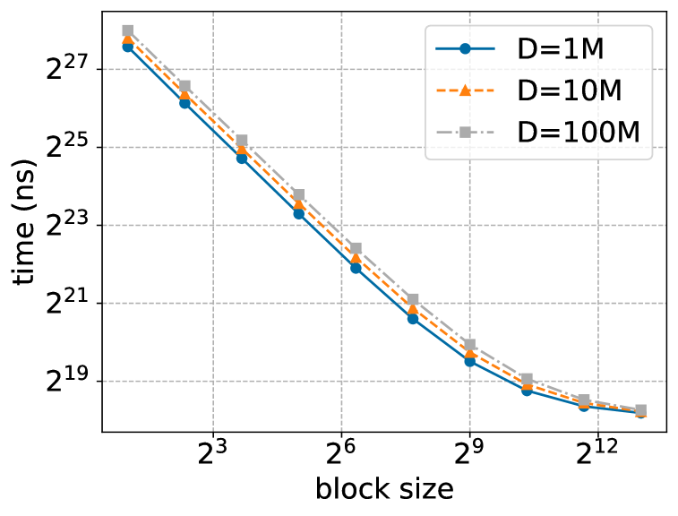
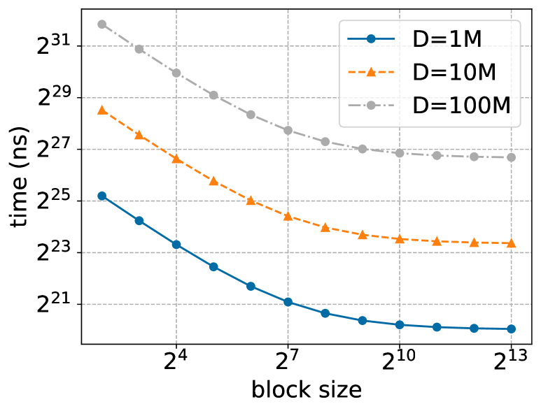
Figure 8: PRG call time for client (left) and server (right) in PREAMBLE

Communication.

Figure 9 shows the required communication, or DPF key size, for the same parameter settings as the times reported in Figure 8. Note that the communication scales with $B,k,$ and $D$ as the client computation. This communication is the same as what would be necessary for in the block-sparse DPF construction. We also include a baseline communication comparison, which is the minimum communication required to communicate $kB$ group elements of size $\log|\mathbb{G}|=\lambda$ and the $D/B$ indices of the non-zero blocks. Except for the factor of 3 communication overhead from cuckoo hashing, the communication converges to approximately that of the baseline by block size around 1000. As alluded to above, this $3\times$ overhead can be reduced to a constant much closer to $1$, if one uses more than $2$ hash functions. E.g. using 3 (resp. 4) hash functions reduces the overhead to $1.1\times$ (resp. $1.03\times$), at the cost of increased server computation.

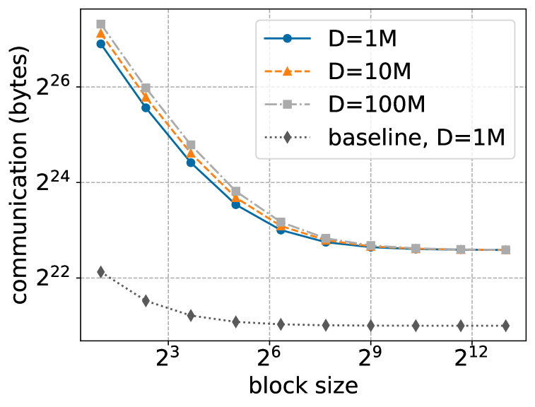
Figure 9: Communication for PREAMBLE

4 Private aggregation via $k$-block-sparse vectors

In this section we propose two instantiations of our sampling-based sparsification, and describe the formal privacy and utility guarantees of the resulting aggregation algorithms. In both schemes each user is given a vector $v\in\mathbb{R}^{D}$ which consists of $\Delta=D/B$ blocks, each of size $B$. We refer to the value of $v$ on block $i\in[\Delta]$ by $v_{i}\in\mathbb{R}^{B}$. Our subsampling schemes are parametrized by an upper bound on the norm of each block $L$ and the number of blocks $k$ to be sent by each user. We will also assume, for simplicity, that $k$ divides $\Delta$. The bound $L$ would typically by $O(\sqrt{B/D})$ if the full vector has norm $1$, and this can be ensured by converting the vector to its Kashin representation [LV10], or by applying a suitably random rotation. A shared randomized Hadamard Transform can achieve this goal efficiently (see e.g.  [AFN⁺23]). We note that requiring the block norms are controlled is a much weaker requirement than the coordinate norms being controlled, and thus this property is easier to enforce for larger $B$. We evaluate this in  Section 4.1.

We present two subsampling schemes, which differ in how the $k$ blocks are subsampled. In Fig. 10, we partition the blocks into $k$ groups, and pick one block out of each group, randomly and independently. In Fig. 11, we select each block with probability $q$, to get in expectation $q\Delta$ blocks. If the number of blocks that end up getting subsampled is larger than $k$, we keep at random $k$ of them. This gives at most $k$ non-zero blocks, which can be communicated using PREAMBLE. Both schemes give about the same expected utility, and privacy bounds that match asymptotically. The partitioned subsampling results in a more structured $k$-block-sparse vector, which is a concatenation of $k$ $1$-block-sparse vectors, which are simpler to communicate. The truncated Poisson subsampling has more randomness, and can be analyzed numerically using a larger set of tools, though it may have slightly higher communication cost. As we discuss in Section 4.1, each of these may be preferable over the other for some range of parameters.

SampledVector (Partitioned Subsampling) Input: vector $v\in\mathbb{R}^{D}$. Parameters: dimension $D$, blocksize $B$, sparsity $k$, $\Delta=D/B$, blockwise $\ell_{2}$ bound $L$. 1. Split the block indices into $k$ consecutive subsets $S_{j}=\{(j-1)\Delta/k+1,\ldots,j\Delta/k\}$ for $j\in[k]$. 2. Select an index $i_{j}$ randomly and uniformly from $S_{j}$ and define $I=\{i_{j}\}_{j\in[k]}$ 3. Define the subsampled (and clipped) $v^{I}$ as $$v^{I}_{i}=\begin{cases}\frac{\Delta}{k}\cdot\mbox{clip}_{L}(v_{i})&\text{if }i\in I\\ 0&\text{otherwise}\end{cases},$$ where $\mbox{clip}_{L}(z)$ is defined as $z$ if $\|z\|_{2}\leq L$ and $\frac{L}{\|z\|_{2}}\cdot z$, otherwise. 4. Output $w=v^{I}$.

Figure  10: $k$-wise 1-sparse sampling scheme

SampledVector (Truncated Poisson Subsampling) Input: vector $v\in\mathbb{R}^{D}$. Parameters: dimension $D$, blocksize $B$, sparsity $k$, sampling probability $q$, $\Delta=D/B$, blockwise $\ell_{2}$ bound $L$. 1. Select a subset $I_{0}$ by picking each coordinate in $\{1,\ldots,\Delta\}$ independently with probability $q$. 2. If $|I_{0}|>k$, let $I$ be random subset of $I_{0}$ of size $k$. Else set $I=I_{0}$. 3. Let $\kappa=\mathop{\mathbb{E}}[|I|]=\mathop{\mathbb{E}}[\min(\texttt{Bin}(\Delta,q),k)]$ under this sampling process. 4. Define the subsampled (and clipped) $v^{I}$ as $$v^{I}_{i}=\begin{cases}\frac{\Delta}{\kappa}\cdot\mbox{clip}_{L}(v_{i})&\text{if }i\in I\\ 0&\text{otherwise}\end{cases}.$$ 5. Output $w=v^{I}$.

Figure  11: $k$-sparse sampling scheme

Theorem 6 (Utility of the subsampling schemes).

Let $v^{1},\ldots,v^{n}$ be a collection of vectors such that each $v^{j}=v^{j}_{1},\ldots,v^{j}_{\Delta}\in\mathbb{R}^{D}$ and $\|v^{j}_{i}\|_{2}\leq L$ for all $j\in[n]$ and $i\in[\Delta]$. Let $w^{j}$ denote the (randomized) report of either of our subsampling algorithms for each $j\in[n]$ and let $W=\sum_{j\in[n]}w^{j}+N(\bar{0},\sigma^{2}I_{D})$ be their noisy aggregate. Then

$$\mathbf{E}[\|W-\sum_{j\in[n]}v^{j}\|_{2}^{2}]\leq nL^{2}\frac{\Delta^{2}}{k}+\sigma^{2}\cdot D.$$

Proof.

First, note that $\mathbf{E}[w^{j}]=v^{j}$ for all $j\in[n]$. Therefore we have

$$\mathbf{E}[\|W-\sum_{j\in[n]}v^{j}\|_{2}^{2}] =\mathbf{E}\left[\|\sum_{j\in[n]}w^{j}-v^{j}+N(\bar{0},\sigma^{2}I_{D})\|_{2}^{2}\right]$$

$$=\sum_{j=1}^{n}\mathbf{E}\left[\|w^{j}-v^{j}\|_{2}^{2}\right]+\sigma^{2}D$$

$$=n\mathbf{E}\left[\|w^{1}-v^{1}\|_{2}^{2}\right]+\sigma^{2}D$$

$$\leq n\Delta\tfrac{k}{\Delta}(1-\tfrac{k}{\Delta})L^{2}(\frac{\Delta}{k})^{2}+\sigma^{2}D$$

$$\leq n\cdot L^{2}(\Delta^{2}/k)+\sigma^{2}D.$$

Here we have used the fact that the variance of the $w^{1}$ decomposes across $\Delta$ blocks, where each block contributed $p(1-p)$ times the square of its value when non-zero (which is $L(\Delta/k)$) and $p=\tfrac{k}{\Delta}$ is the probability of a block being non-zero. ∎

Theorem 6 provides guidance on how to set the smallest communication cost so that the sub-sampling error is negligible compared to the privacy error. Indeed, assume for simplicity that our vectors lie in the $\ell_{\infty}$-ball $v^{j}\in\left[\frac{-1}{\sqrt{D}},\frac{1}{\sqrt{D}}\right]^{D}$. This implies that the norm of each block is upper bounded by $L=\sqrt{B/D}$. Noting that $\Delta=D/B$, the (upper bound above on the) error of the algorithm is $n\Delta/k+\sigma^{2}D$. This implies that we should set $kB\geq c\cdot n/\sigma^{2}$ for some constant $c>0$. In other words, the number of coordinates that are non-zero must be set to $cn/\sigma^{2}$, which is independent on $D$, as well as of the blocksize. Thus block-based subsampling does not impact the sampling noise, and any setting of $k$ and $B$ with the product $kB\geq cn/\sigma^{2}$ would suffice.

We also note that the proof is oblivious to the subsampling method and only uses the fact that marginally, each coordinate has the right expectation, and is non-zero with probability $k/\Delta$. Thus it applies to a range of subsampling methods.

We now analyze the privacy of our subsampling methods using the standard notion of differential privacy [DMNS06] with respect to deletion of user data. In the context of aggregation, we can also think of this adjacency notion as replacing the user’s data with the all-0 vector. We state the asymptotic privacy guarantees for our partitioned subsampling method below (the proof can be found in Appendix B). Similar guarantees hold for the Truncated Poisson subsampling with an appropriate choice of parameters and can be derived from the known analyses [ACG⁺16, Ste22] together with the fact that the truncation operation does not degrade the privacy guarantees [FS25].

Theorem 7 (Privacy of partitioned subsampling).

Let $v^{1},\ldots,v^{n}$ be a collection of vectors such that each $v^{j}=v^{j}_{1},\ldots,v^{j}_{\Delta}\in\mathbb{R}^{D}$ and $\|v^{j}_{i}\|_{2}\leq L$ for all $j\in[n]$ and $i\in[\Delta]$. Let $w^{j}$ denote the (randomized) report using Partitioned Subsampling, for each $j\in[n]$ and let $A$ be an algorithm that outputs $W=\sum_{j\in[n]}w^{j}+N(\bar{0},\sigma^{2}I_{D})$. Then there exists a constant $c$ such that for every $\delta>0$, if

$$\frac{\sigma}{L}\geq c\cdot\max\left\{\frac{\Delta\sqrt{\log(\Delta/\delta)}}{k},\sqrt{\frac{\Delta}{k}}\log(\Delta/\delta),\sqrt{\Delta\log(1/\delta)}\right\},$$

then $A$ is $(\epsilon,\delta)$-differentially private for

$$\varepsilon=O\left(\frac{L\sqrt{\Delta}\sqrt{\log(1/\delta)}}{\sigma}\right).$$

Note that this implies that when $L=\sqrt{1/\Delta}$ and we set $kB$ to be $n/\sigma^{2}$, the resulting $\varepsilon$ is $O(\sqrt{\log(1/\delta)}/\sigma)$, which asymptotically matches the bound for the Gaussian mechanism. In other words, the privacy cost of our algorithm is close to that of the Gaussian mechanism, when $kB\geq n/\sigma^{2}$ and $k\geq\sqrt{\Delta\log\frac{1}{\delta}}/\sigma$. For a fixed $kB$, this constraint translates to an upper bound on the block size.

This asymptotic analysis demonstrates the importance of hiding the sparsity pattern. Specifically, without hiding the pattern we cannot appeal to privacy amplification by subsampling and need to rely on the sensitivity of the aggregated value. The sensitivity is equal to $\sqrt{k}\cdot\frac{L\Delta}{k}=\frac{L\Delta}{\sqrt{k}}$. By the properties of the Gaussian noise addition (Thm. 2), we obtain that the algorithm is $\left(O\left(\frac{L\Delta\sqrt{\log(1/\delta)}}{\sigma\sqrt{k}}\right),\delta\right)$-DP. This bound is worse by a factor of $\sqrt{\frac{\Delta}{k}}$ than the bound we get in Theorem 7. A similar gain was obtained for private aggregation of Poisson subsampled vectors in [CSOK23].

Communicating $1$-sparse vectors:

A common application of secure aggregation systems is to aggregate vectors that are $1$-sparse (often known as $1$-hot vectors) or $k$-sparse for a small $k$. Directly using DPFs for these vectors requires $O(D)$ PRG re-seedings and thus can be expensive. Noting that $k$-sparse vector is also $k$-block sparse, one can directly use PREAMBLE to reduce the server computation cost at a modest increase in communication cost. Alternately, in settings where we want to add noise in a distributed setting, RAPPOR [EPK14] and its lower-communication variants such as PI-RAPPOR [FT21] and ProjectiveGeometryResponse [FNNT22] can be used along with Prio. Since $1$-hot vectors become vectors in $\left\{\frac{1}{\sqrt{D}},\frac{-1}{\sqrt{D}}\right\}^{D}$ after a Hadamard transform, one can view these vectors as Euclidean vectors in $\mathbb{R}^{D}$ and use PREAMBLE to efficiently communicate them. ProjectiveGeometryResponse is particularly well-suited for this setup even without sampling, as the resulting message space is $O(D)$-dimensional, and a linear transformation of the input space. Thus one can aggregate in “message space”: each message is a $1$-hot vector in message space, and we can add up these vectors using PREAMBLE. The linear transform to go back to data space is a simple post-processing and the privacy guarantee here can use privacy amplification by shuffling. Since we avoid sampling in this approach, it can scale to larger $n$ without incurring any additional utility overhead.

4.1 Numerical Privacy Analysis

As discussed above, under appropriate assumptions on the block size, we can prove asymptotic privacy guarantee for our approach that matches that of the Gaussian mechanism itself. In this section, we evaluate the privacy-utility trade-off of our approach using numerical techniques to compute the privacy cost.

We will analyze the two approaches described above. For both schemes, the noise due to subsampling can be upper bounded using Theorem 6. For partitioned subsampling, we use the recent work on Privacy Amplification by Random Allocation [FS25] to analyze the privacy cost. The authors show that the Renyi DP parameters of the one-out-of-$m$ version of the Gaussian mechanism can be bounded using numerical methods. Composing this across the $k$ groups gives us the Renyi DP parameters, and hence the overall privacy cost of the full mechanism.

For the approach based on truncated Poisson subsampling, it is shown in [FS25] that the privacy cost is no larger than that of the Poisson subsampling version without the truncation. The Poisson subsampling can then be analyzed using the PRV accountant of  [GLW21]. While the PRV accountant usually gives better bounds than one can get from RDP-based accounting, we suffer a multiplicative overhead as the scaling factor $\kappa$ in Truncated Poisson is smaller than $k$. For the numerical analysis, we optimize over $q$ to control the overall variance one gets from this process. Note that when $k$ is large and $q\approx\frac{k-O(\sqrt{k})}{\Delta}$, one would expect truncation to be rare, and thus $\kappa$ to be close to $q\Delta$ and thus to $k$.

One can also study a different subsampling process where $I$ is a uniformly random subset of size $k$. We may expect better privacy bounds to hold for this version, intuitively as there is more randomness compared to partitioned subsampling. Feldman and Shenfeld [FS25] show that the privacy bound of this variant is no larger than that of partitioned subsampling. We conjecture that the privacy cost of this version is closer to (untruncated) Poisson with sampling rate $q=k/\Delta$. Since the latter can be more precisely accounted for using the PRV accountant, we expect careful numerical accounting of this version to do better than the RDP-based bounds for partitioned subsampling.

For our baseline Gaussian mechanism, we use the Analytic Gaussian mechanism analysis from [WBK21]. For these numerical results, we assume that $L$ is fixed to $\sqrt{B/D}$. For each of the approaches, we compute the total variance of the error in the sum, which includes the privacy error that results from the numerical privacy analysis, and the sampling error as bounded by Theorem 6. For the communication cost, we simply plot $kB$ as it is a good proxy for the actual communication cost for a large range of parameters. Based on the evaluation in Section 3, we consider values of $B$ that are in the range $(2^{10},2^{14})$.

Fig. 12 shows the trade-off between communication cost and the standard deviation of the error for our algorithm, using partitioned subsampling, as well as the Gaussian baseline. As is clear from the plots, our approach allows us to significantly reduce the communication costs, at the price of a minor increase in the error. This holds for a range of $D$ from 1M to 8M, and for a range of $\varepsilon$ values. In Fig. 13, we explore the trade-off between the standard deviation of the error and the privacy budget for different communication budget. Finally, in Fig. 14 we compare the performance of the partitioned subsampling scheme and the truncated Poisson, where the plots show that each method is favorable in different regimes: the truncated Poisson obtains better error if more communication is allowed, getting closer to the error of the Gaussian mechanism. This is partly due to the analysis of partitioned subsampling building on RDP analysis, which even for the Gaussian mechanism yields standard deviation bounds slightly larger than the analytic Gaussian mechanism. The truncated Poisson analysis uses the tighter PRV accounting.

As we decrease the communication $kB$, the error in Fig. 12 essentially stays constant until a point, and then rapidly increases. This is largely due to the fact that for large block sizes, the norm of each block is larger so that the required lower bound on $\sigma$ to ensure privacy amplification by subsampling is larger. While the plots are derived from the numerical analysis which is tighter, intuition for this can be derived from the condition $k>\sqrt{\Delta\log 1/\delta}/\sigma$, or equivalently $\sigma>\sqrt{\Delta\log 1/\delta}/k$ in Theorem 7. Thus for the case of small $kB$, one would prefer smaller block sizes. Our plots show that blocksizes in the range $[2^{10},2^{13}]$ provide low error across a range of parameters. Recall that in Figs. 8 and 9, we saw that block sizes above $2^{10}$ are sufficient to get most of the communication and computation benefits.

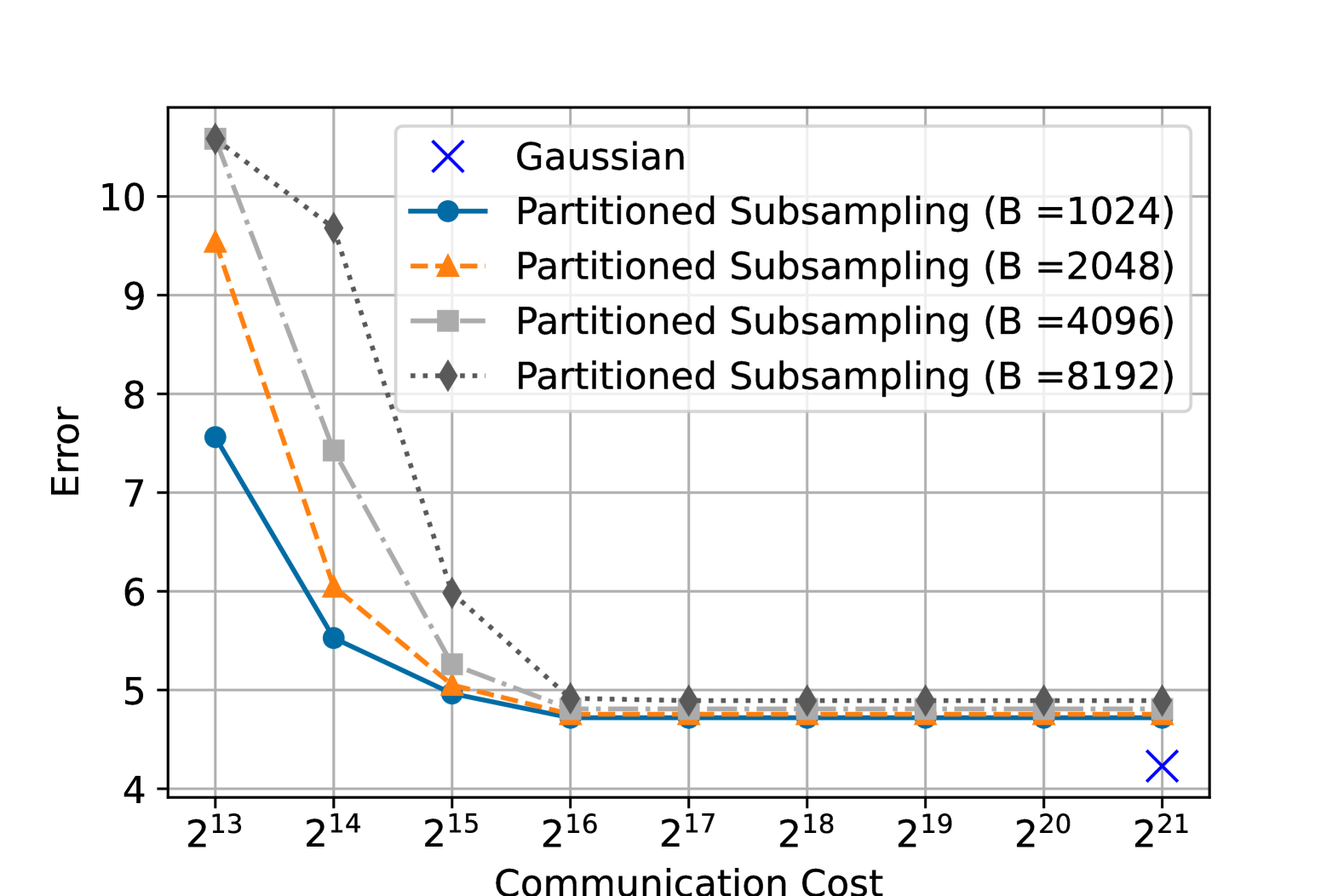
(a)

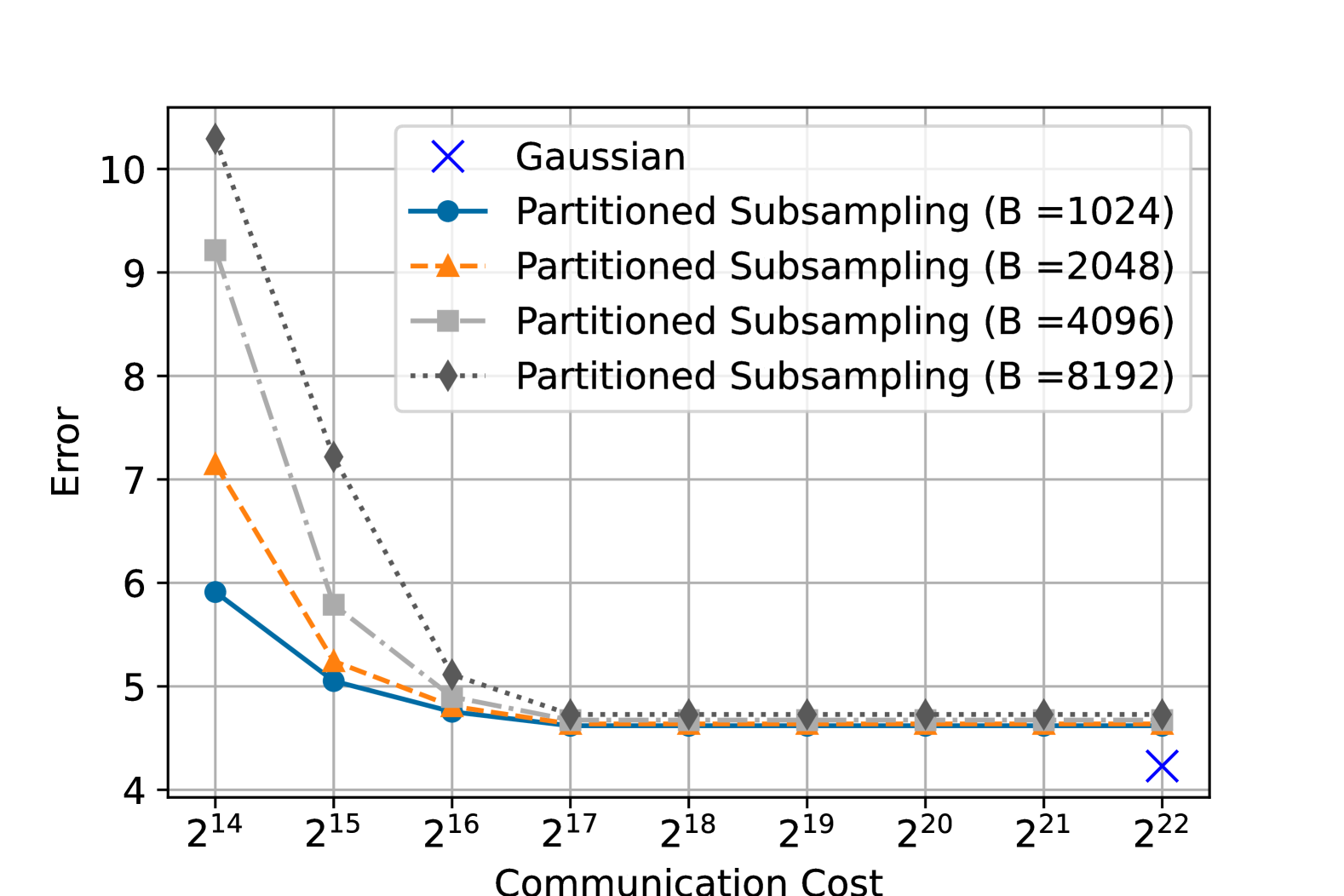
(b)

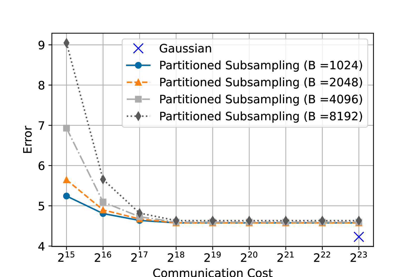
(c)

Figure 12: The trade-off between the standard deviation of the error and per-client communication $C=kB$, when computing the sum of $n=10^{5}$ vectors with dimension (a) $D=2^{21}$, (b) $D=2^{22}$, and (c) $D=2^{23}$, with $(1.0,10^{-6})$-DP. The blue ’x’ shows the baseline approach of sending the whole vector.

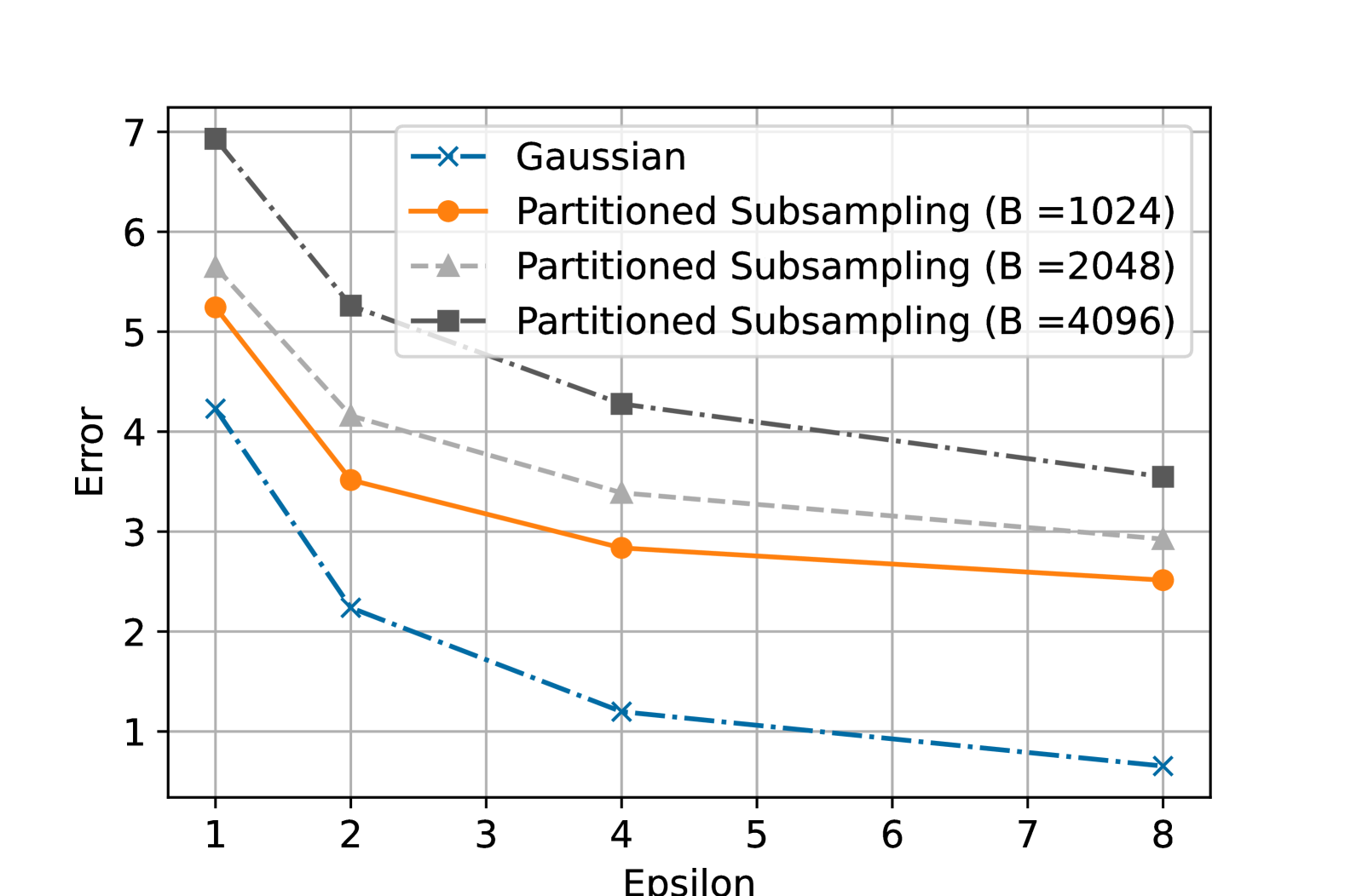
(a)

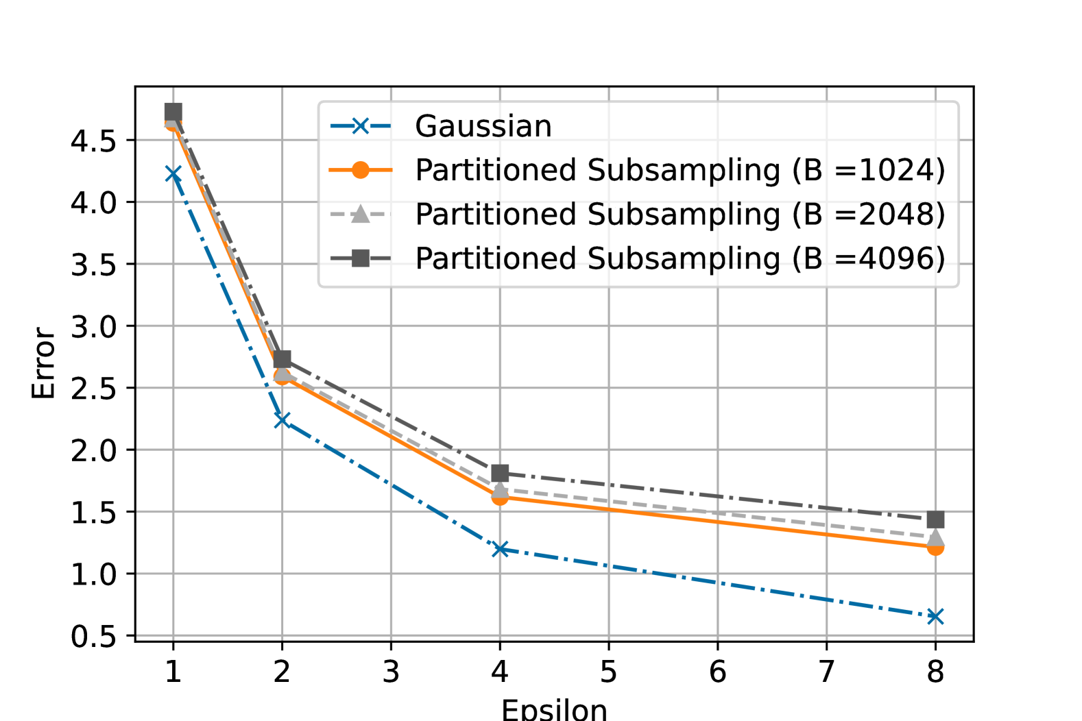
(b)

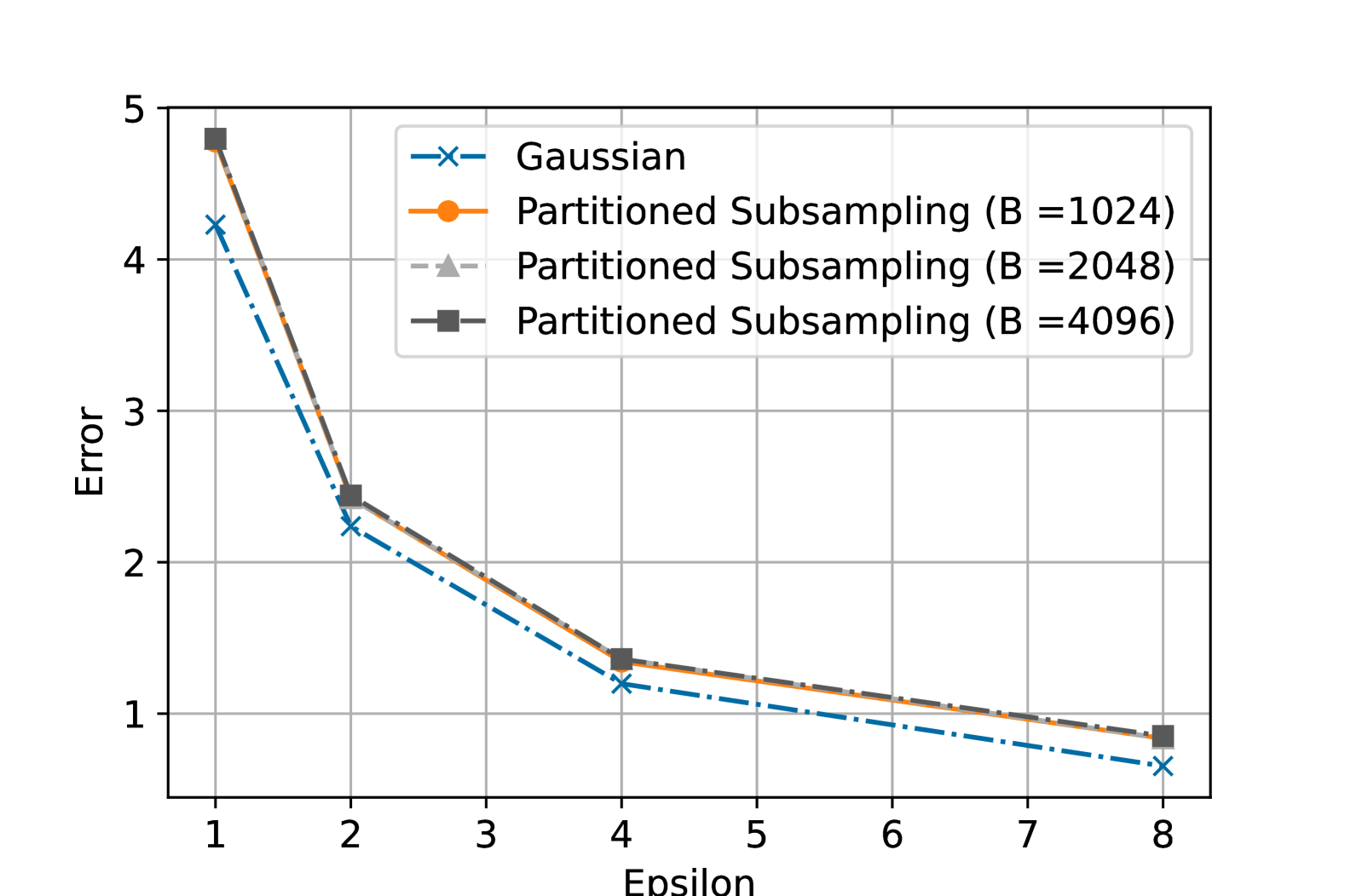
(c)

Figure 13: The trade-off between the standard deviation of the error and privacy budget for varying communication complexity $C=kB$ where (a) small $C=2^{15}$, (b) intermediate $C=2^{17}$, or (c) large $C=2^{19}$. The number of vectors is $n=10^{5}$ with dimension $D=2^{23}$.

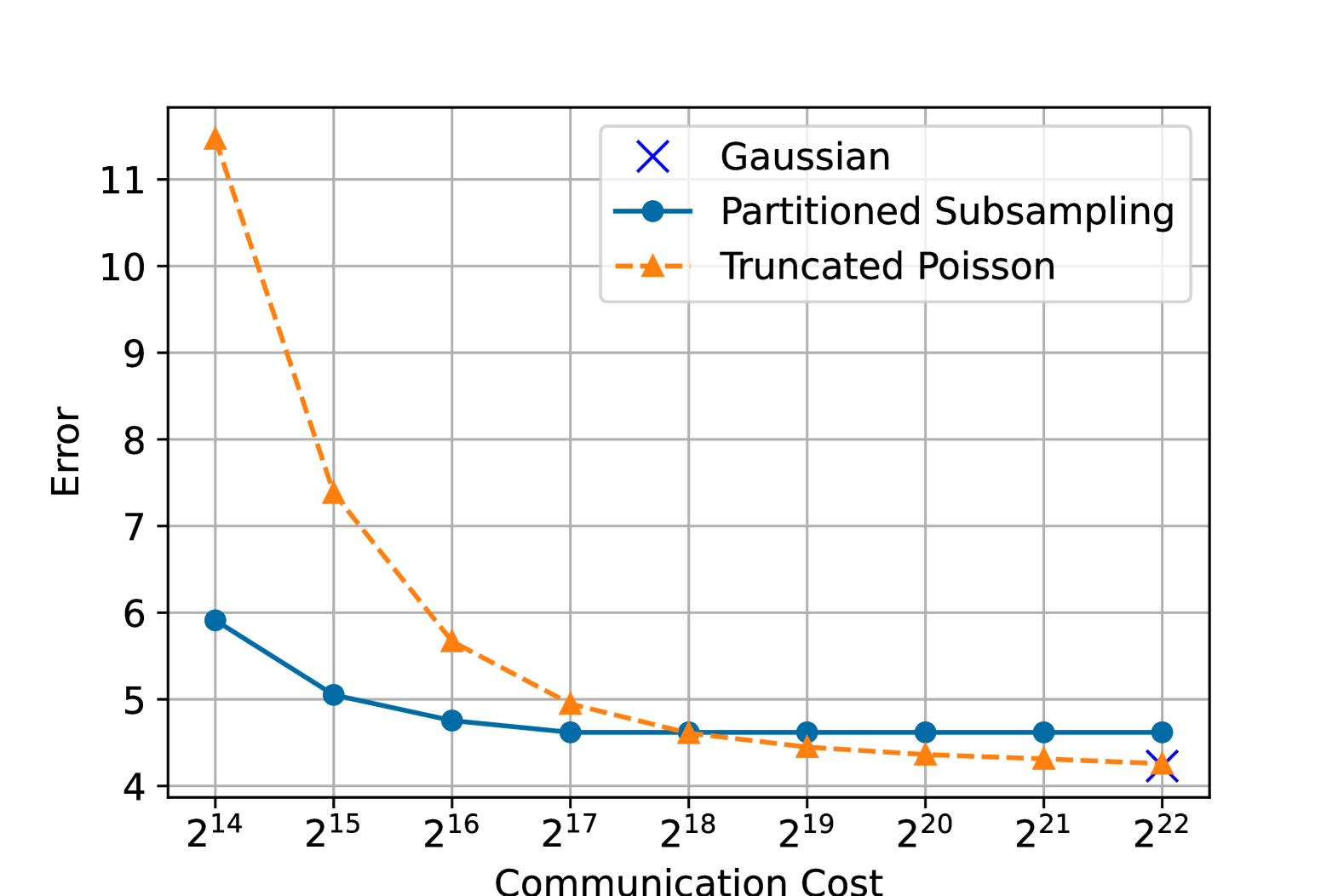
(a)

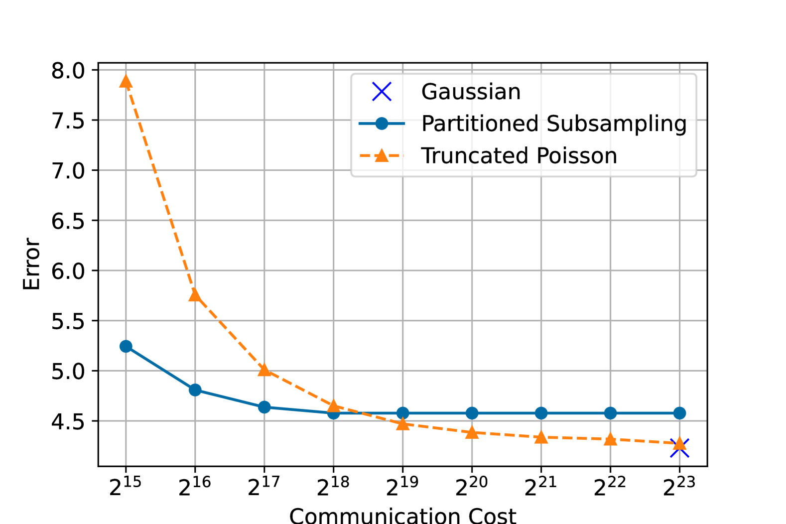
(b)

Figure 14: The trade-off between the standard deviation of the error and per-client communication for the Partitioned Subsampling scheme and the Truncated Poisson. These plots are for aggregating $n=10^{5}$ vectors with dimension (a) $D=2^{22}$, (b) $D=2^{23}$, block size $B=2^{10}$ and $(1.0,10^{-6})$-DP.

Finally, we analyze empirically the ease of ensuring a block-wise norm bound. Theoretically, a norm bound of $O(\frac{1}{\sqrt{D}}$ on each entry can be ensured if one transforms to a $O(D)$-dimensional space; the hidden constants in the two $O(\cdot)$ notations are related, where making one smaller makes the other larger. In practice, a simple approach often used is to apply a random rotation to the vector, followed by truncating any entry that is larger than $\frac{c}{\sqrt{D}}$, for an appropriate constant $c$. For moderate values of $c$, the truncation error (i.e. the norm of the induced error) is small for a random rotation). Imposing the weaker condition that each block has $\ell_{2}$ norm at most $\frac{c}{\sqrt{D/B}}$ results in a lower truncation error. In Fig. 15, we plot the truncation error as a function of $c$, when we apply a random rotation, for different values of the block size $B$. It is easy to see that $c<1$ will result in non-trivial truncation error for any block size. Our plots show that even moderately large $B$ allow us to take $c$ very close to $1$ for a negligible truncation error.

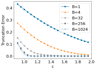
(a)

(b)

Figure 15: The trade-off between the truncation error $\|Trunc_{c}(Gv)-Gv\|_{2}$ and constant $c$, where $v\in\mathbb{R}^{D}$ is arbitrary, and $G$ is a random rotation matrix. The plots show the error for various block sizes, for (a) $D=2^{15}$ and (b) $D=2^{20}$.

5 Conclusions

In this work, we have described PREAMBLE, an efficient algorithm for communicating high-dimensional $k$-block sparse vectors in the Prio model. We showed how to construct zero-knowledge proofs to validate a bound on the Euclidean norm and $k$-block-sparsity of these vectors. Our algorithms require client communication proportional to the sparsity $kB$ of these vectors, and our client computation also scales only with $kB$ for parameters of interest. Our construction allows the servers to reconstruct each contribution using $O(D)$ field operations and PRG evaluations in counter mode, and a significantly smaller number of the more expensive PRG reseeding operations. We also showed how PREAMBLE combines with random sampling, and privacy amplification-by-sampling type analyses to significantly improve the communication complexity of differentially private vector aggregation with a small overhead in accuracy.

We leave open some natural research directions. Our numerical privacy analyses, while close to tight, still leave some gaps, and it would be natural to improve those. In particular, the $k$-out-of-$\Delta$ sampling approach should admit privacy analyses better than the partitioning based approach, and we conjecture that the privacy cost of this approach is no worse than the Poisson sampling based method. Our approach based on Cuckoo hashing with two hash functions incurs a constant factor communication overhead, and has a $O(\frac{1}{k})$ failure probability. While the overhead can be reduced by using a few more hash function, the failure probability of cuckoo hashing remains $k^{-c}$ for a small constant $c$ (see e.g. [KMW08]). While for our application to approximate aggregation, this has little impact, it would be natural to design a version of our scheme that has a negligible failure probability.

Appendix A Proof of Theorem 4

Correctness.

We describe and argue correctness of our optimized $k$-block-sparse DPF construction in a way that is analogous to our arguments for the original construction of [BGI16]. The invariant for the $k$-sparse case is that in layer $i$ of the tree construction, the $\tilde{k}$ nodes corresponding to $\alpha_{i}$ are non-zero, and all others are zero. In addition, we maintain the invariant that exactly one of the two bit components on the non-zero path is 1, and the other is 0. More formally, we would like that if $x\notin\alpha_{i}$, $s_{i}(x)=t_{i}(x)$, $u_{i}(x)=v_{i}(x)$, and $q_{i}(x)=r_{i}(x)$. Furthermore, we would like that for $x\in\alpha_{i}$, exactly one of $u_{i}(x)=v_{i}(x)$, and $q_{i}(x)=r_{i}(x)$ should hold.

The function $h_{i}:[2^{i-1}]\rightarrow[3k]^{2}$ maps one $\alpha^{\ell}_{i}$ in tree layer $i$ to two correction words. We use cuckoo hashing to determine which of these two correction words will be applied for $\alpha^{\ell}_{i}$, defining function $g_{i}:[2^{i-1}]\rightarrow\{0,1\}$. Due to cuckoo hashing, we know that this mapping exists for any $k$-block-sparse function given all $h_{i}$ with probability $1-\mathcal{O}(\frac{1}{k})$. In the upper levels, the PRG $G:\{0,1\}^{\lambda}\rightarrow\{0,1\}^{2\lambda+4}$ output is parsed as follows:

$$s^{\prime}_{i+1}(x||0)||u^{\prime}_{i+1}(x||0)||q^{\prime}_{i+1}(x||0)||s^{\prime}_{i+1}(x||1)||u^{\prime}_{i+1}(x||1)||q^{\prime}_{i+1}(x||1) =G(s_{i}(x))$$

$$t^{\prime}_{i+1}(x||0)||v^{\prime}_{i+1}(x||0)||r^{\prime}_{i+1}(x||0)||t^{\prime}_{i+1}(x||1)||v^{\prime}_{i+1}(x||1)||r^{\prime}_{i+1}(x||1) =G(t_{i}(x))$$

In the original construction, the seed portion of the correction word was set in such a way as to set to zero the node corresponding to $\alpha_{i}||\bar{b}_{i}$, where $\bar{b}_{i}$ is defined such that $\alpha_{i+1}\neq\alpha_{i}||\bar{b}_{i}$. Let us now analogously define $\bar{b}_{i}^{\ell}$, defined such that $\alpha_{i+1}^{\ell}\neq\alpha_{i}^{\ell}||\bar{b}_{i}^{\ell}$. It is possible that there exist indices $\ell\neq\ell^{\prime}\in[k]$ such that $\alpha^{\ell}_{i}||\bar{b}_{i}^{\ell}=\alpha^{\ell^{\prime}}_{i+1}$, in which case we do not want to set the seed portion of the node corresponding to $\alpha^{\ell}_{i}||\bar{b}_{i}^{\ell}$ to 0. For such an $\ell$, we set the seed portion of the corresponding correction word to a random bit-string instead. For other $\ell$, we set the corresponding seed correction, specified by the $g_{i}(\alpha_{i}^{\ell})$th output of $h_{i}(\alpha_{i}^{\ell})$, as expected:

$$c_{h_{i+1}(\alpha_{i}^{\ell})[g_{i}(\alpha_{i}^{\ell})]}=s^{\prime}_{i+1}(\alpha^{\ell}_{i}||\bar{b}_{i}^{\ell})+t^{\prime}_{i+1}(\alpha^{\ell}_{i}||\bar{b}_{i}^{\ell})$$

The corrected seed components are then for each $x\in\{0,1\}^{i}$ and $b\in\{0,1\}$:

$$s_{i+1}(x||b)=s^{\prime}_{i+1}(x||b)-u_{i}(x)c_{h_{i+1}(x)[0]}-q_{i}(x)c_{h_{i+1}(x)[1]}$$

$$t_{i+1}(x||b)=t^{\prime}_{i+1}(x||b)-v_{i}(x)c_{h_{i+1}(x)[0]}-r_{i}(x)c_{h_{i+1}(x)[1]}$$

It is then easy to check that for $x\neq\alpha_{i}^{\ell}$ for all $\ell\in[k]$, the equalities $u_{i}(x)=v_{i}(x)$ and $q_{i}(x)=r_{i}(x)$ imply that $s_{i+1}(x||b)=t_{i+1}(x||b)$. Moreover for $y=\alpha_{i}^{\ell}||\bar{b}_{i}^{\ell}$, as long as $y\notin\alpha_{i+1}$, we have

$$s_{i+1}(y)-t_{i+1}(y) =s^{\prime}_{i+1}(y)-u_{i}(\alpha^{\ell}_{i})c_{h_{i+1}(\alpha_{i}^{\ell})[0]}-q_{i}(\alpha^{\ell}_{i})c_{h_{i+1}(\alpha_{i}^{\ell})[1]}$$

$$~~~-(t^{\prime}_{i+1}(y)-v_{i}(\alpha^{\ell}_{i})c_{h_{i+1}(\alpha_{i}^{\ell})[0]}-r_{i}(\alpha^{\ell}_{i})c_{h_{i+1}(\alpha_{i}^{\ell})[1]})$$

$$=s^{\prime}_{i+1}(y)-t^{\prime}_{i+1}(y)-(u_{i}(\alpha^{\ell}_{i})-v_{i}(\alpha^{\ell}_{i}))c_{h_{i+1}(\alpha_{i}^{\ell})[0]}$$

$$~~~-(q_{i}(\alpha^{\ell}_{i})-r_{i}(\alpha^{\ell}_{i}))c_{h_{i+1}(\alpha_{i}^{\ell})[1]}$$

$$=s^{\prime}_{i+1}(y)-t^{\prime}_{i+1}(y)-1c_{h_{i+1}(\alpha_{i}^{\ell})[g_{i+1}(\alpha_{i}^{\ell})]}$$

$$=0.$$

Here the last step follows by definition of $c_{h_{i+1}(\alpha_{i}^{\ell})[g_{i+1}(\alpha_{i}^{\ell})]}$.

Finally, we need to correct the new bit components. For this purpose, we compute two bit corrections. Note that $u_{i+1}(y)=v_{i+1}(y)$ and $q_{i+1}(y)=r_{i+1}(y)$ for each $y\notin\alpha_{i+1}$. On the other hand, when $y\in\alpha_{i+1}$, we would like either $u_{i+1}(y)=v_{i+1}(y)$ and $q_{i+1}(y)\neq r_{i+1}(y)$ or $u_{i+1}(y)\neq v_{i+1}(y)$ and $q_{i+1}(y)=r_{i+1}(y)$, depending on $g_{i+1}(y)$. We set the bit corrections to:

$$m_{h_{i+1}(\alpha_{i}^{\ell})[g_{i+1}(\alpha_{i}^{\ell})]}(0)=u^{\prime}_{i+1}(\alpha_{i}^{\ell}||0)-v^{\prime}_{i+1}(\alpha_{i}^{\ell}||0)+(g_{i+2}(\alpha_{i}^{\ell}||0)+1)(\alpha^{\ell}_{i}||0\in\alpha_{i+1})$$

$$m_{h_{i+1}(\alpha_{i}^{\ell})[g_{i+1}(\alpha_{i}^{\ell})]}(1)=u^{\prime}_{i+1}(\alpha_{i}^{\ell}||1)-v^{\prime}_{i+1}(\alpha_{i}^{\ell}||1)+(g_{i+2}(\alpha_{i}^{\ell}||1)+1)(\alpha^{\ell}_{i}||1\in\alpha_{i+1})$$

$$p_{h_{i+1}(\alpha_{i}^{\ell})[g_{i+1}(\alpha_{i}^{\ell})]}(0)=q^{\prime}_{i+1}(\alpha_{i}^{\ell}||0)-r^{\prime}_{i+1}(\alpha_{i}^{\ell}||0)+g_{i+2}(\alpha_{i}^{\ell}||0)(\alpha^{\ell}_{i}||0\in\alpha_{i+1})$$

$$p_{h_{i+1}(\alpha_{i}^{\ell})[g_{i+1}(\alpha_{i}^{\ell})]}(1)=q^{\prime}_{i+1}(\alpha_{i}^{\ell}||1)-r^{\prime}_{i+1}(\alpha_{i}^{\ell}||1)+g_{i+2}(\alpha_{i}^{\ell}||1)(\alpha^{\ell}_{i}||1\in\alpha_{i+1})$$

To apply the bit correction, the following is computed:

$$u_{i+1}(x||b)=u^{\prime}_{i+1}(x||b)-u_{i}(x)m_{h_{i+1}(x)[0]}(b)-q_{i}(x)m_{h_{i+1}(x)[1]}(b)$$

$$v_{i+1}(x||b)=v^{\prime}_{i+1}(x||b)-v_{i}(x)m_{h_{i+1}(x)[0]}(b)-r_{i}(x)m_{h_{i+1}(x)[1]}(b)$$

$$q_{i+1}(x||b)=q^{\prime}_{i+1}(x||b)-u_{i}(x)p_{h_{i+1}(x)[0]}(b)-q_{i}(x)p_{h_{i+1}(x)[1]}(b)$$

$$r_{i+1}(x||b)=r^{\prime}_{i+1}(x||b)-v_{i}(x)p_{h_{i+1}(x)[0]}(b)-r_{i}(x)p_{h_{i+1}(x)[1]}(b)$$

The correctness proof is identical to the one for the $s-t$ case when $x||b\notin\alpha_{i+1}$. Otherwise, when $x||b\in\alpha_{i+1}$, we show that

$$u_{i+1}(x||b)-v_{i+1}(x||b) =u^{\prime}_{i+1}(x||b)-u_{i}(x)m_{h_{i+1}(x)[0]}(b)-q_{i}(x)m_{h_{i+1}(x)[1]}(b)$$

$$~~~-(v^{\prime}_{i+1}(x||b)-v_{i}(x)m_{h_{i+1}(x)[0]}(b)-r_{i}(x)m_{h_{i+1}(x)[1]}(b))$$

$$=u^{\prime}_{i+1}(x||b)-v^{\prime}_{i+1}(x||b)-(u_{i}(x)-v_{i}(x))m_{h_{i+1}(x)[0]}(b)$$

$$~~~-(q_{i}(x)r_{i}(x))m_{h_{i+1}(x)[1]}(b)$$

$$=u^{\prime}_{i+1}(x||b)-v^{\prime}_{i+1}(x||b)-m_{h_{i+1}(x)[g_{i+1}(x)]}(b)$$

$$=g_{i+2}(\alpha_{i}^{\ell}||b)+1$$

Using analogous arguments, $q_{i+1}(x||b)-r_{i+1}(x||b)=g_{i+2}(\alpha_{i}^{\ell}||b)$. Therefore, exactly one of either $u_{i+1}(x||b)=v_{i+1}(x||b)$ or $q_{i+1}(y)=r_{i+1}(y)$ can hold, and the required invariant is maintained.

In the lowest layer, the PRG is evaluated for each $\ell\in[k]$:

$$s^{\prime}_{d+1}(\alpha^{\ell}||0)||\dots||s^{\prime}_{d+1}(\alpha^{\ell}||B-1)=G^{\prime}(s_{d}(\alpha^{\ell}))$$

$$t^{\prime}_{d+1}(\alpha^{\ell}||0)||\dots||t^{\prime}_{d+1}(\alpha^{\ell}||B-1)=G^{\prime}(t_{d}(\alpha^{\ell}))$$

In a next step, we call the $convert(\cdot)$ function on each component of these outputs. The goal is to formulate one correction word for each of the $k$ non-zero blocks.

More formally, we would like to choose correction words $c_{h_{d+1}(\alpha^{\ell})[g_{d+1}(\alpha^{\ell})]}(j)$ for $j\in[B]$ such that ${s}_{d+1}(\alpha^{\ell}||j)-{t}_{d+1}(\alpha^{\ell}||j)=\beta_{j}^{\ell}$:

$${s}_{d+1}(\alpha^{\ell}||j) =s^{\prime}_{d+1}(\alpha^{\ell}||j)+u_{d}(\alpha^{\ell})c_{h_{d+1}(\alpha^{\ell})[0]}(j)+q_{d}(\alpha^{\ell})c_{h_{d+1}(\alpha^{\ell})[1]}(j)$$

$${t}_{d+1}(\alpha^{\ell}||j) =t^{\prime}_{d+1}(\alpha^{\ell}||j)+v_{d}(\alpha^{\ell})c_{h_{d+1}(\alpha^{\ell})[1]}(j)+r_{d}(\alpha^{\ell})c_{h_{d+1}(\alpha^{\ell})[1]}(j).$$

Note that for $x\not\in\alpha$, $s^{\prime}_{d+1}(x||j)=t^{\prime}_{d+1}(x||j)$, $u_{d}(x)=v_{d}(x)$, and $q_{d}(x)=r_{d}(x)$, so ${s}_{d+1}(x||j)={t}_{d+1}(x||j)$ for all $j\in[B]$, regardless of the correction words.

For $\alpha^{\ell}$, if $g_{d+1}(\alpha^{\ell})=0$, then $u_{d}(\alpha^{\ell})\neq v_{d}(\alpha^{\ell})$ and $q_{d}(\alpha^{\ell})=r_{d}(\alpha^{\ell})$. Otherwise, $q_{d}(\alpha^{\ell})\neq r_{d}(\alpha^{\ell})$ and $u_{d}(\alpha^{\ell})=v_{d}(\alpha^{\ell})$. Exactly one of ${s}_{d+1}(x||j)$ and ${t}_{d+1}(x||j)$ is independent of $c_{h_{d+1}(\alpha^{\ell})[g_{d+1}(\alpha^{\ell})]}$. By subtracting over $\mathbb{G}$, we can find the target value of the other one and choose the correction word accordingly.

In a bit more detail: the client computes the sequence
$(s^{\prime}_{d+1}(\alpha^{\ell}||j)-t^{\prime}_{d+1}(\alpha^{\ell}||j))_{j\in[B]}\in\mathbb{G}$. It computes the seed correction for each $j\in[B]$ and send it to both servers.. If $g_{d+1}(\alpha^{\ell})=0$

$$c_{h_{d+1}(\alpha^{\ell})[g_{d+1}(\alpha^{\ell})]}(j)=(u_{d,\ell}(\alpha^{\ell})-v_{d,\ell}(\alpha^{\ell}))^{-1}(\beta^{\ell}_{j}-(s^{\prime}_{d+1}(\alpha^{\ell}||j)-t^{\prime}_{d+1}(\alpha^{\ell}||j)))$$

Otherwise:

$$c_{h_{d+1}(\alpha^{\ell})[g_{d+1}(\alpha^{\ell})]}(j)=(q_{d}(\alpha^{\ell})-r_{d}(\alpha^{\ell}))^{-1}(\beta^{\ell}_{j}-(s^{\prime}_{d+1}(\alpha^{\ell}||j)-t^{\prime}_{d+1}(\alpha^{\ell}||j)))$$

Since $(u_{d}(\alpha^{\ell})-v_{d}(\alpha^{\ell})),(q_{d}(\alpha^{\ell})-r_{d}(\alpha^{\ell}))\in\{-1,0,1\}$, the inverse over $\mathbb{G}$ is well defined.

Now for $x=\alpha^{\ell}$, we can write

$${s} {}_{d+1}(\alpha^{\ell}||j)-{t}_{d+1}(\alpha^{\ell}||j)$$

$$=s^{\prime}_{d+1}(\alpha^{\ell}||j)-t^{\prime}_{d+1}(\alpha^{\ell}||j)+(u_{d}(\alpha^{\ell})-v_{d}(\alpha^{\ell}))c_{h_{d+1}(\alpha^{\ell})[0]}(j)$$

$$~~~+(q_{d}(\alpha^{\ell})-r_{d}(\alpha^{\ell}))c_{h_{d+1}(\alpha^{\ell})[1]}(j)$$

$$=s^{\prime}_{d+1}(\alpha^{\ell}||j)-t^{\prime}_{d+1}(\alpha^{\ell}||j)+(\beta^{\ell}_{j}-s^{\prime}_{d+1}(\alpha^{\ell}||j)+t^{\prime}_{d+1}(\alpha^{\ell}||j))$$

$$=\beta^{\ell}_{j}.$$

Security.

We argue that each server’s DPF key is pseudorandom. The security proof is analogous to the proof of Theorem 3.3 in [BGI16]. We begin by describing the high-level argument. Each server begins with a random seed, which is unknown to the other server. In each tree layer, up to $k$ random seeds are expanded using a PRG, generating 2 new seeds and 4 bits, all of which appear similarly random due to the security of the PRG and the fact that the original seed appeared random. The application of a correction word will cancel the randomness of 5 of these 6 resulting seed and bit components. Specifically, one seed component and all 4 bit components are canceled; however, given only the correction word and the tree node values held by a single server, the resulting secret shares still appear random.

It is possible to define a series of hybrids $Hyb_{w,\ell}$, where the correction words in all levels $i<w$ are replaced by random bit strings for $i\in[d+1]$, replacing Step 2 in Figure 6, the first $\ell$ correction word components in layer $w$ are replaced by a random bit string, and if $w=d+1$ the first $\ell$ components of the final level correction word are replaced with random group elements, replacing Step 10 in Figure 5. We also consider the view of the first of the two servers, without loss of generality. Specifically:

1. Choose $s_{0}(0),t_{0}(0),u_{0}(0),v_{0}(0),q_{0}(0),r_{0}(0)$ honestly.

2. Choose $CW^{0},\dots,CW^{w-1}\in\{0,1\}^{3k(\lambda+4)}$ uniformly at random.

3. Choose $CW^{w}$ such that the first $\ell$ components are uniform samples and the remaining ones are computed honestly.

4. Update $s_{i}(\alpha_{i}^{\ell})$, $u_{i}(\alpha_{i}^{\ell})$, $q_{i}(\alpha_{i}^{\ell})$ honestly for all $i<w$ and $\ell\in[\tilde{k}]$.

5. For $i=w$, set $t_{i}(\alpha_{i}^{0})$,$v_{i}(\alpha_{i}^{0})$,$r_{i}(\alpha_{i}^{0}),\dots,t_{i}(\alpha_{i}^{\ell})$,$v_{i}(\alpha_{i}^{\ell})$,$r_{i}(\alpha_{i}^{\ell})$ to random values. Also set to random values the terms $t_{i-1}(\alpha_{i-1}^{\ell+1})$,$v_{i-1}(\alpha_{i-1}^{\ell+1})$,$r_{i-1}(\alpha_{i-1}^{\ell+1}),\dots,t_{i-1}(\alpha_{i-1}^{\tilde{k}-1})$,$v_{i-1}(\alpha_{i-1}^{\tilde{k}-1})$,$r_{i-1}(\alpha_{i-1}^{\tilde{k}-1})$. Compute $t_{i}(\alpha_{i}^{\ell+1})$,$v_{i}(\alpha_{i}^{\ell+1})$,$r_{i}(\alpha_{i}^{\ell+1}),\dots,t_{i}(\alpha_{i}^{\tilde{k}-1})$,$v_{i}(\alpha_{i}^{\tilde{k}-1})$,$r_{i}(\alpha_{i}^{\tilde{k}-1})$ honestly.

6. For $i>w$, compute all $CW^{i}$ and update all $s_{i}(\alpha_{i}^{\ell})$, $t_{i}(\alpha_{i}^{\ell})$, $u_{i}(\alpha_{i}^{\ell})$, $v_{i}(\alpha_{i}^{\ell})$, $q_{i}(\alpha_{i}^{\ell})$, $r_{i}(\alpha_{i}^{\ell})$ honestly for all $\ell\in[k]$.

7. The output is $s_{0}(0),u_{0}(0),q_{0}(0)||CW^{1}||\dots||CW^{d+1}$.

Note that when $w=\ell=0$, this experiment corresponds to the honest key distribution, whereas when $w=d+1,\ell=k-1$ this yields a completely random key. We claim that each pair of adjacent hybrids will be indistinguishable based on the security of the pseudorandom generator.

We first consider $w\leq d$ and a $Hyb$-distinguishing adversary $\mathcal{A}$ who distinguishes $Hyb_{w,\ell}$ from either $Hyb_{w,\ell+1}$ if $\ell<\tilde{k}-1$ or $Hyb_{w+1,0}$ otherwise. Given an adversary $\mathcal{A}$ with advantage $\rho$, we can construct a corresponding PRG adversary $\mathcal{B}$. This PRG adversary is given a value $r\in\{0,1\}^{2(\lambda+2)}$ and distinguishes between the cases where $r$ is truly random and $r=G(s)$, where $s\in\{0,1\}^{\lambda}$ is a random seed. Given $\alpha,\beta,w,\ell$, the adversary $\mathcal{B}$ constructs a DPF key according to $Hyb_{w,\ell}$; however, instead of sampling $t_{w}(\alpha^{\ell}_{w}),v_{w}(\alpha^{\ell}_{w}),r_{w}(\alpha^{\ell}_{w})$ randomly, we set:

$$t_{w} (\alpha^{\ell}_{w-1}||0)||v_{w}(\alpha^{\ell}_{w-1}||0)||r_{w}(\alpha^{\ell}_{w-1}||0)||t_{w}(\alpha^{\ell}_{w-1}||1)||v_{w}(\alpha^{\ell}_{w-1}||1)||r_{w}(\alpha^{\ell}_{w-1}||1)$$

to $r$. If $r$ is computed pseudorandomly, then it is clear that the resulting DPF key is generated as in $Hyb_{w,\ell}(1^{\lambda},\alpha,\beta)$. We must also argue that if $r$ is random, the resulting key is distributed as in either $Hyb_{w,\ell+1}$ if $\ell<\tilde{k}-1$ or $Hyb_{w+1,0}$ otherwise. If $t_{w}(\alpha^{\ell}_{w}),v_{w}(\alpha^{\ell}_{w}),r_{w}(\alpha^{\ell}_{w})$ is random, then the corresponding correction word is also uniformly random, since it is computed as the xor of a fixed bit-string with these randomly selected bit-strings, forming a perfect one-time pad. After applying this correction word, the resulting seed and bit components are also uniformly distributed, given only the previous seed and bit components for that server, as well as the correction words.

Combining these pieces, an adversary $\mathcal{A}$ that distinguishes between the hybrids with advantage $\rho$ yields a corresponding adversary $\mathcal{B}$ for the PRG experiment with the same advantage and only polynomial additional runtime.

Finally, we consider $w=d+1$. We can make an argument similar to the previous one that an adversary that distinguishes between the distributions $Hyb_{d+1,\ell}$ and $Hyb_{d+1,\ell+1}$ with advantage $\rho$ directly yields a corresponding adversary $\mathcal{B}$ for the pseudo-randomness of the PRG output, interpreted as a group element, with the same advantage and only polynomial additional runtime. $\mathcal{B}$ can embed the challenge by setting the corresponding correction word to $(-1)^{r_{i-1}(\alpha_{i-1}^{\ell})}(\beta_{j}^{\ell}-s_{i}^{\prime}(\alpha_{i-1}^{\ell}||j)+r)$. If $r$ is generated pseudo-randomly, this is exactly the distribution of $Hyb_{d+1,\ell}$. If $r$ is truly random, then it similarly acts as a one-time pad on the remaining terms and the corresponding correction word is uniformly distributed, as in $Hyb_{d+1,\ell+1}$.

Appendix B Proof of Theorem 7

We will need the following asymptotic bound on the privacy of Poisson subsampling of the Gaussian noise addition.

Lemma B.1 ([ACG⁺16]).

Let $A_{1},\ldots,A_{T}:(\mathbb{R}^{B})^{n}\rightarrow\mathbb{R}^{B}$ be a sequence of Gaussian noise addition algorithms with sensitivity $s$ and noise scale $\sigma$. Let $P_{\eta}(A_{1},\ldots,A_{T})$ be the Poisson subsampling scheme in which each user’s data is used in each step with probability $\eta$ randomly and independently (of other users and steps). Then, there exist a constant $c$ such that for every $\delta>0$, if $\sigma/s\geq c\eta\sqrt{T\log(1/\delta)}$ then $P_{\eta}(A_{1},\ldots,A_{T})$ satisfies $(\varepsilon,\delta)$-DP for $\varepsilon=O(\eta\frac{s}{\sigma}\sqrt{T\log(1/\delta)}$.

Proof of Theorem 7.

We first observe that we can analyze algorithm as an independent composition of $A_{1},\ldots,A_{k}$, with the instance $A_{j}$ outputting the coordinates of $W$ in the set $S_{j}=\{(j-1)\Delta/k+1,\ldots,j\Delta/k\}$ for $j\in[k]$. For convenience of notation we will analyze $A_{1}$ (with the rest being identical). Observe that the output of $A_{1}$ is $W_{1},\ldots,W_{\Delta/k}$. Now, by the definition of the sampling scheme, any user’s data is summed in exactly one (uniformly chosen) of $W_{1},\ldots,W_{\Delta/k}$. Each of these algorithms is Gaussian noise addition with sensitivity $L\Delta/k$ and scale $\sigma$. This implies that we can apply results for privacy amplification by allocation for Gaussian noise from [FS25] to analyze this algorithm. For the analytic results we use an upper bound on the privacy parameters of random allocation in terms of Poisson subsampling for Gaussian noise. Specifically, for every $\varepsilon$, $k$-wise composition of 1 out of $\Delta/k$ random allocation for Gaussian noise addition algorithms satisfies $(\varepsilon,\delta_{P}+\Delta\delta_{0}+\delta^{\prime})$-DP, where $(\varepsilon,\delta_{P})$ are the privacy parameters of $\Delta$-step Poisson subsampling scheme with rate $\eta=\frac{k}{\Delta(1-\gamma)}$ for $\gamma=(e^{\varepsilon_{0}}-e^{\varepsilon_{0}})\sqrt{\frac{k}{2\Delta}\ln\left(\frac{k}{\delta^{\prime}}\right)}$. Here $(\varepsilon_{0},\delta_{0})$ are the privacy parameters of each Gaussian noise addition. Note that the sensitivity of the aggregate in each block is $L\Delta/k$. Therefore, setting $\delta_{0}=\delta/(3\Delta)$ we get $\varepsilon_{0}=\frac{L\Delta\sqrt{2\ln(15\Delta/(4\delta))}}{k\sigma}$ (Thm. 2). We set $\delta^{\prime}=\delta/3$ and note that by the first part of our assumption on $\sigma/L$, $\varepsilon_{0}\leq 1$ and therefore $e^{\varepsilon_{0}}-e^{\varepsilon_{0}}\leq 3\varepsilon_{0}$. Now the second part of our assumption of $\sigma/L$ implies that

$$\gamma \leq 3\varepsilon_{0}\sqrt{\frac{k}{2\Delta}\ln\left(\frac{3k}{\delta}\right)}$$

$$\leq\frac{3L\Delta\sqrt{2\ln(15\Delta/(4\delta))}}{k\sigma}\sqrt{\frac{k}{2\Delta}\ln\left(\frac{3k}{\delta}\right)}$$

$$\leq\frac{3L\sqrt{\Delta}\ln(15\Delta/(4\delta))}{\sqrt{k}\sigma}\leq 1/2.$$

This implies that $\eta\leq\frac{2k}{\Delta}$. Now, by Lemma B.1, the $\Delta$-step Poisson subsampling scheme with subsampling rate $\eta$ is $(\varepsilon,\delta/3)$-DP for

$$\varepsilon=O\left(\frac{L\sqrt{\Delta}\sqrt{\log(1/\delta)}}{\sigma}\right).$$

Here we note that the conditions of the lemma translate to

$$\frac{\sigma k}{L\Delta}\geq c\frac{k}{\Delta}\sqrt{\Delta\log(1/\delta)}$$

or equivalently, $\frac{\sigma}{L}\geq c\sqrt{\Delta\log(1/\delta)}$ (which is ensured by the third part of our assumption). Finally, noting that $\Delta\delta_{0}+\delta^{\prime}\leq 2\delta/3$, we get the claimed bound. ∎

References

- [AC06] Nir Ailon and Bernard Chazelle. Approximate nearest neighbors and the fast johnson-lindenstrauss transform. In Proceedings of the Thirty-Eighth Annual ACM Symposium on Theory of Computing, STOC ’06, page 557–563, New York, NY, USA, 2006. Association for Computing Machinery.
- [ACG+16] Martín Abadi, Andy Chu, Ian J. Goodfellow, H. Brendan McMahan, Ilya Mironov, Kunal Talwar, and Li Zhang. Deep learning with differential privacy. In Edgar R. Weippl, Stefan Katzenbeisser, Christopher Kruegel, Andrew C. Myers, and Shai Halevi, editors, ACM CCS 2016, pages 308–318. ACM Press, October 2016.
- [ACLS18] Sebastian Angel, Hao Chen, Kim Laine, and Srinath T. V. Setty. PIR with compressed queries and amortized query processing. In 2018 IEEE Symposium on Security and Privacy, pages 962–979. IEEE Computer Society Press, May 2018.
- [AFN+23] Hilal Asi, Vitaly Feldman, Jelani Nelson, Huy Nguyen, and Kunal Talwar. Fast optimal locally private mean estimation via random projections. In A. Oh, T. Naumann, A. Globerson, K. Saenko, M. Hardt, and S. Levine, editors, Advances in Neural Information Processing Systems, volume 36, pages 16271–16282. Curran Associates, Inc., 2023.
- [AFN+24] Hilal Asi, Vitaly Feldman, Jelani Nelson, Huy L. Nguyen, Kunal Talwar, and Samson Zhou. Private vector mean estimation in the shuffle model: Optimal rates require many messages, 2024.
- [AFT22] Hilal Asi, Vitaly Feldman, and Kunal Talwar. Optimal algorithms for mean estimation under local differential privacy. In International Conference on Machine Learning, ICML, USA, pages 1046–1056, 2022.
- [AG21] Apple and Google. Exposure notification privacy-preserving analytics (ENPA) white paper. https://covid19-static.cdn-apple.com/applications/covid19/current/static/contact-tracing/pdf/ENPA_White_Paper.pdf, 2021.
- [AGJ+22] Surya Addanki, Kevin Garbe, Eli Jaffe, Rafail Ostrovsky, and Antigoni Polychroniadou. Prio+: Privacy preserving aggregate statistics via boolean shares. In Clemente Galdi and Stanislaw Jarecki, editors, Security and Cryptography for Networks - 13th International Conference, SCN 2022, Amalfi, Italy, September 12-14, 2022, Proceedings, volume 13409 of Lecture Notes in Computer Science, pages 516–539. Springer, 2022.
- [APF+23] Sheikh Shams Azam, Martin Pelikan, Vitaly Feldman, Kunal Talwar, Jan Silovsky, and Tatiana Likhomanenko. Federated learning for speech recognition: Revisiting current trends towards large-scale ASR. In International Workshop on Federated Learning in the Age of Foundation Models in Conjunction with NeurIPS 2023, 2023.
- [AS19] Jayadev Acharya and Ziteng Sun. Communication complexity in locally private distribution estimation and heavy hitters. In Proceedings of the 36th International Conference on Machine Learning, ICML, pages 51–60, 2019.
- [BBC+19] Dan Boneh, Elette Boyle, Henry Corrigan-Gibbs, Niv Gilboa, and Yuval Ishai. Zero-knowledge proofs on secret-shared data via fully linear pcps. In Alexandra Boldyreva and Daniele Micciancio, editors, Advances in Cryptology - CRYPTO 2019 - 39th Annual International Cryptology Conference, Santa Barbara, CA, USA, August 18-22, 2019, Proceedings, Part III, volume 11694 of Lecture Notes in Computer Science, pages 67–97. Springer, 2019.
- [BBC+23] Dan Boneh, Elette Boyle, Henry Corrigan-Gibbs, Niv Gilboa, and Yuval Ishai. Arithmetic sketching. In Helena Handschuh and Anna Lysyanskaya, editors, CRYPTO 2023, Part I, volume 14081 of LNCS, pages 171–202. Springer, Cham, August 2023.
- [BBCG+21] Dan Boneh, Elette Boyle, Henry Corrigan-Gibbs, Niv Gilboa, and Yuval Ishai. Lightweight techniques for private heavy hitters. In 2021 IEEE Symposium on Security and Privacy (S & P), pages 762–776, 2021.
- [BBG20] Borja Balle, Gilles Barthe, and Marco Gaboardi. Privacy profiles and amplification by subsampling. Journal of Privacy and Confidentiality, 10(1), 2020.
- [BBGN19] Borja Balle, James Bell, Adrià Gascón, and Kobbi Nissim. The privacy blanket of the shuffle model. In Advances in Cryptology - CRYPTO 2019 - 39th Annual International Cryptology Conference, Proceedings, Part II, pages 638–667, 2019.
- [BBGN20] Borja Balle, James Bell, Adrià Gascón, and Kobbi Nissim. Private summation in the multi-message shuffle model. In CCS ’20: 2020 ACM SIGSAC Conference on Computer and Communications Security, pages 657–676, 2020.
- [BCGI18] Elette Boyle, Geoffroy Couteau, Niv Gilboa, and Yuval Ishai. Compressing vector OLE. In David Lie, Mohammad Mannan, Michael Backes, and XiaoFeng Wang, editors, ACM CCS 2018, pages 896–912. ACM Press, October 2018.
- [BCPS25] Richard Barnes, David Cook, Christopher Patton, and Phillipp Schoppmann. Verifiable Distributed Aggregation Functions. Internet-Draft draft-irtf-cfrg-vdaf-14, Internet Engineering Task Force, January 2025. Work in Progress.
- [BDF+18] Abhishek Bhowmick, John C. Duchi, Julien Freudiger, Gaurav Kapoor, and Ryan Rogers. Protection against reconstruction and its applications in private federated learning. CoRR, abs/1812.00984, 2018.
- [BGI15] Elette Boyle, Niv Gilboa, and Yuval Ishai. Function secret sharing. In Elisabeth Oswald and Marc Fischlin, editors, EUROCRYPT 2015, Part II, volume 9057 of LNCS, pages 337–367. Springer, Berlin, Heidelberg, April 2015.
- [BGI16] Elette Boyle, Niv Gilboa, and Yuval Ishai. Function secret sharing: Improvements and extensions. In Edgar R. Weippl, Stefan Katzenbeisser, Christopher Kruegel, Andrew C. Myers, and Shai Halevi, editors, ACM CCS 2016, pages 1292–1303. ACM Press, October 2016.
- [BNO08] Amos Beimel, Kobbi Nissim, and Eran Omri. Distributed private data analysis: Simultaneously solving how and what. In David Wagner, editor, Advances in Cryptology – CRYPTO 2008, pages 451–468, Berlin, Heidelberg, 2008. Springer Berlin Heidelberg.
- [BS15] Raef Bassily and Adam D. Smith. Local, private, efficient protocols for succinct histograms. In Proceedings of the Forty-Seventh Annual ACM on Symposium on Theory of Computing, STOC, pages 127–135, 2015.
- [BS16] Mark Bun and Thomas Steinke. Concentrated differential privacy: Simplifications, extensions, and lower bounds. In Martin Hirt and Adam Smith, editors, Theory of Cryptography, pages 635–658, Berlin, Heidelberg, 2016. Springer Berlin Heidelberg.
- [BW18] Borja Balle and Yu-Xiang Wang. Improving the gaussian mechanism for differential privacy: Analytical calibration and optimal denoising. In International Conference on Machine Learning, 2018.
- [CB17] Henry Corrigan-Gibbs and Dan Boneh. Prio: Private, robust, and scalable computation of aggregate statistics. In Aditya Akella and Jon Howell, editors, 14th USENIX Symposium on Networked Systems Design and Implementation, NSDI 2017, Boston, MA, USA, March 27-29, 2017, pages 259–282. USENIX Association, 2017.
- [CCT+24] Geeticka Chauhan, Steve Chien, Om Thakkar, Abhradeep Thakurta, and Arun Narayanan. Training large asr encoders with differential privacy. In 2024 IEEE Spoken Language Technology Workshop (SLT), pages 102–109. IEEE, 2024.
- [CGH+25] Lynn Chua, Badih Ghazi, Charlie Harrison, Pritish Kamath, Ravi Kumar, Ethan Jacob Leeman, Pasin Manurangsi, Amer Sinha, and Chiyuan Zhang. Balls-and-bins sampling for DP-SGD. In The 28th International Conference on Artificial Intelligence and Statistics, 2025.
- [CIK+24] Wei-Ning Chen, Berivan Isik, Peter Kairouz, Albert No, Sewoong Oh, and Zheng Xu. Improved communication-privacy trade-offs in l2 mean estimation under streaming differential privacy. In Proceedings of the 41st International Conference on Machine Learning, ICML’24. JMLR.org, 2024.
- [CJMP22] Albert Cheu, Matthew Joseph, Jieming Mao, and Binghui Peng. Shuffle private stochastic convex optimization. In The Tenth International Conference on Learning Representations, ICLR, 2022.
- [CKÖ20] Wei-Ning Chen, Peter Kairouz, and Ayfer Özgür. Breaking the communication-privacy-accuracy trilemma. arXiv preprint arXiv:2007.11707, 2020.
- [CLR17] Hao Chen, Kim Laine, and Peter Rindal. Fast private set intersection from homomorphic encryption. In Bhavani M. Thuraisingham, David Evans, Tal Malkin, and Dongyan Xu, editors, ACM CCS 2017, pages 1243–1255. ACM Press, October / November 2017.
- [CMS11] Kamalika Chaudhuri, Claire Monteleoni, and Anand D. Sarwate. Differentially private empirical risk minimization. Journal of Machine Learning Research, 12(29):1069–1109, 2011.
- [CSOK23] Wei-Ning Chen, Dan Song, Ayfer Ozgur, and Peter Kairouz. Privacy amplification via compression: Achieving the optimal privacy-accuracy-communication trade-off in distributed mean estimation. In Thirty-seventh Conference on Neural Information Processing Systems, 2023.
- [CSS12] T. H. Hubert Chan, Elaine Shi, and Dawn Song. Privacy-preserving stream aggregation with fault tolerance. In Angelos D. Keromytis, editor, Financial Cryptography and Data Security, pages 200–214, Berlin, Heidelberg, 2012. Springer Berlin Heidelberg.
- [DJW18] John C. Duchi, Michael I. Jordan, and Martin J. Wainwright. Minimax optimal procedures for locally private estimation. Journal of the American Statistical Association, 113(521):182–201, 2018.
- [DK12] Michael Drmota and Reinhard Kutzelnigg. A precise analysis of cuckoo hashing. ACM Trans. Algorithms, 8(2), April 2012.
- [DKM+06] Cynthia Dwork, Krishnaram Kenthapadi, Frank McSherry, Ilya Mironov, and Moni Naor. Our data, ourselves: Privacy via distributed noise generation. In Advances in Cryptology (EUROCRYPT 2006), volume 4004 of Lecture Notes in Computer Science, pages 486–503. Springer Verlag, 2006.
- [DMNS06] Cynthia Dwork, Frank McSherry, Kobbi Nissim, and Adam Smith. Calibrating noise to sensitivity in private data analysis. In Shai Halevi and Tal Rabin, editors, Theory of Cryptography, pages 265–284, Berlin, Heidelberg, 2006. Springer Berlin Heidelberg.
- [DPRS23] Hannah Davis, Christopher Patton, Mike Rosulek, and Phillipp Schoppmann. Verifiable distributed aggregation functions. Cryptology ePrint Archive, Report 2023/130, 2023.
- [DR14] Cynthia Dwork and Aaron Roth. The algorithmic foundations of differential privacy. Found. Trends Theor. Comput. Sci., 9(3-4):211–407, 2014.
- [DR16] Cynthia Dwork and Guy N. Rothblum. Concentrated differential privacy. CoRR, abs/1603.01887, 2016.
- [DR19] John C. Duchi and Ryan Rogers. Lower bounds for locally private estimation via communication complexity. In Conference on Learning Theory, COLT, pages 1161–1191, 2019.
- [DRRT18] Daniel Demmler, Peter Rindal, Mike Rosulek, and Ni Trieu. PIR-PSI: Scaling private contact discovery. PoPETs, 2018(4):159–178, October 2018.
- [DRS22] Jinshuo Dong, Aaron Roth, and Weijie J. Su. Gaussian differential privacy. Journal of the Royal Statistical Society Series B: Statistical Methodology, 84(1):3–37, 02 2022.
- [EPK14] Úlfar Erlingsson, Vasyl Pihur, and Aleksandra Korolova. Rappor: Randomized aggregatable privacy-preserving ordinal response. In Proceedings of the 2014 ACM SIGSAC Conference on Computer and Communications Security, CCS ’14, page 1054–1067, New York, NY, USA, 2014. Association for Computing Machinery.
- [FHNP16] Michael J. Freedman, Carmit Hazay, Kobbi Nissim, and Benny Pinkas. Efficient set intersection with simulation-based security. Journal of Cryptology, 29(1):115–155, January 2016.
- [FM12] Alan Frieze and Páll Melsted. Maximum matchings in random bipartite graphs and the space utilization of cuckoo hash tables. Random Structures & Algorithms, 41(3):334–364, 2012.
- [FNNT22] Vitaly Feldman, Jelani Nelson, Huy Nguyen, and Kunal Talwar. Private frequency estimation via projective geometry. In Kamalika Chaudhuri, Stefanie Jegelka, Le Song, Csaba Szepesvari, Gang Niu, and Sivan Sabato, editors, Proceedings of the 39th International Conference on Machine Learning, volume 162 of Proceedings of Machine Learning Research, pages 6418–6433. PMLR, 2022.
- [FP12] Nikolaos Fountoulakis and Konstantinos Panagiotou. Sharp load thresholds for cuckoo hashing. Random Structures & Algorithms, 41(3):306–333, 2012.
- [FPE16] Giulia Fanti, Vasyl Pihur, and Úlfar Erlingsson. Building a RAPPOR with the unknown: Privacy-preserving learning of associations and data dictionaries. Proc. Priv. Enhancing Technol., 2016(3):41–61, 2016.
- [FS25] Vitaly Feldman and Moshe Shenfeld. Privacy amplification by random allocation, 2025.
- [FT21] Vitaly Feldman and Kunal Talwar. Lossless compression of efficient private local randomizers. In Marina Meila and Tong Zhang, editors, ICML, volume 139 of Proceedings of Machine Learning Research, pages 3208–3219. PMLR, 2021.
- [GI14] Niv Gilboa and Yuval Ishai. Distributed point functions and their applications. In Phong Q. Nguyen and Elisabeth Oswald, editors, Advances in Cryptology – EUROCRYPT 2014, pages 640–658, Berlin, Heidelberg, 2014. Springer Berlin Heidelberg.
- [GKKM22] Badih Ghazi, Pritish Kamath, Ravi Kumar, and Pasin Manurangsi. Faster privacy accounting via evolving discretization. In Kamalika Chaudhuri, Stefanie Jegelka, Le Song, Csaba Szepesvari, Gang Niu, and Sivan Sabato, editors, Proceedings of the 39th International Conference on Machine Learning, volume 162 of Proceedings of Machine Learning Research, pages 7470–7483. PMLR, 17–23 Jul 2022.
- [GKM+21] Badih Ghazi, Ravi Kumar, Pasin Manurangsi, Rasmus Pagh, and Amer Sinha. Differentially private aggregation in the shuffle model: Almost central accuracy in almost a single message. In Proceedings of the 38th International Conference on Machine Learning, ICML, pages 3692–3701, 2021.
- [GLW21] Sivakanth Gopi, Yin Tat Lee, and Lukas Wutschitz. Numerical composition of differential privacy. In M. Ranzato, A. Beygelzimer, Y. Dauphin, P.S. Liang, and J. Wortman Vaughan, editors, Advances in Neural Information Processing Systems, volume 34, pages 11631–11642. Curran Associates, Inc., 2021.
- [GMPV20] Badih Ghazi, Pasin Manurangsi, Rasmus Pagh, and Ameya Velingker. Private aggregation from fewer anonymous messages. In Advances in Cryptology - EUROCRYPT 2020 - 39th Annual International Conference on the Theory and Applications of Cryptographic Techniques, Proceedings, Part II, pages 798–827, 2020.
- [Gue12] Shay Gueron. Intel Advanced Encryption Standard (AES) New Instructions Set. Technical report, Intel Corporation, September 2012.
- [HMR18] Robert Helmer, Anthony Miyaguchi, and Eric Rescorla. Testing privacy-preserving telemetry with prio. https://hacks.mozilla.org/2018/10/testing-privacy-preserving-telemetry-with-prio/, 2018.
- [HSW+22] Edward J Hu, Yelong Shen, Phillip Wallis, Zeyuan Allen-Zhu, Yuanzhi Li, Shean Wang, Lu Wang, and Weizhu Chen. LoRA: Low-rank adaptation of large language models. In International Conference on Learning Representations, 2022.
- [JL84] William B. Johnson and Joram Lindenstrauss. Extensions of lipschitz mappings into hilbert space. Contemporary mathematics, 26:189–206, 1984.
- [KH21] Antti Koskela and Antti Honkela. Computing differential privacy guarantees for heterogeneous compositions using fft, 2021.
- [KKEPR24] Erki Külaots, Toomas Krips, Hendrik Eerikson, and Pille Pullonen-Raudvere. Slamp-fss: Two-party multi-point function secret sharing from simple linear algebra. Cryptology ePrint Archive, Report 2024/1394, 2024. https://eprint.iacr.org/2024/1394.pdf.
- [KLN+08] S. P. Kasiviswanathan, H. K. Lee, K. Nissim, S. Raskhodnikova, and A. Smith. What can we learn privately? In 2008 49th Annual IEEE Symposium on Foundations of Computer Science, pages 531–540, 2008.
- [KMW08] Adam Kirsch, Michael Mitzenmacher, and Udi Wieder. More robust hashing: Cuckoo hashing with a stash. In Dan Halperin and Kurt Mehlhorn, editors, Algorithms - ESA 2008, pages 611–622, Berlin, Heidelberg, 2008. Springer Berlin Heidelberg.
- [KOV15] Peter Kairouz, Sewoong Oh, and Pramod Viswanath. Secure multi-party differential privacy. In C. Cortes, N. D. Lawrence, D. D. Lee, M. Sugiyama, and R. Garnett, editors, Advances in Neural Information Processing Systems 28, pages 2008–2016. Curran Associates, Inc., 2015.
- [LV10] Y. Lyubarskii and R. Vershynin. Uncertainty principles and vector quantization. Information Theory, IEEE Transactions on, 56(7):3491–3501, 2010.
- [MM18] Sebastian Meiser and Esfandiar Mohammadi. Tight on budget? tight bounds for r-fold approximate differential privacy. In Proceedings of the 2018 ACM SIGSAC Conference on Computer and Communications Security, CCS ’18, page 247–264, New York, NY, USA, 2018. Association for Computing Machinery.
- [MMR+17] Brendan McMahan, Eider Moore, Daniel Ramage, Seth Hampson, and Blaise Agüera y Arcas. Communication-efficient learning of deep networks from decentralized data. In Proceedings of the 20th International Conference on Artificial Intelligence and Statistics, AISTATS, pages 1273–1282, 2017.
- [MTZ19] Ilya Mironov, Kunal Talwar, and Li Zhang. Rényi differential privacy of the sampled gaussian mechanism. ArXiv, abs/1908.10530, 2019.
- [NXY+16] Thông T. Nguyên, Xiaokui Xiao, Yin Yang, Siu Cheung Hui, Hyejin Shin, and Junbum Shin. Collecting and analyzing data from smart device users with local differential privacy. CoRR, abs/1606.05053, 2016.
- [PR01] Rasmus Pagh and Flemming Friche Rodler. Cuckoo hashing. In Proceedings of the 9th Annual European Symposium on Algorithms, ESA ’01, page 121–133, Berlin, Heidelberg, 2001. Springer-Verlag.
- [PSZ14] Benny Pinkas, Thomas Schneider, and Michael Zohner. Faster private set intersection based on OT extension. In Kevin Fu and Jaeyeon Jung, editors, USENIX Security 2014, pages 797–812. USENIX Association, August 2014.
- [ROCT24] Guy N. Rothblum, Eran Omri, Junye Chen, and Kunal Talwar. PINE: Efficient verification of a euclidean norm bound of a Secret-Shared vector. In 33rd USENIX Security Symposium (USENIX Security 24), pages 6975–6992, Philadelphia, PA, August 2024. USENIX Association.
- [RSWP22] Mayank Rathee, Conghao Shen, Sameer Wagh, and Raluca Ada Popa. ELSA: secure aggregation for federated learning with malicious actors. IACR Cryptol. ePrint Arch., page 1695, 2022.
- [RU23] Olivia Röhrig and Maxim Urschumzew. dpsa4fl: Differential privacy for federated machine learning with PRIO, 2023.
- [SFZ+14] Chongjing Sun, Yan Fu, Junlin Zhou, Hui Gao, et al. Personalized privacy-preserving frequent itemset mining using randomized response. The Scientific World Journal, 2014, 2014.
- [SGRR19] Phillipp Schoppmann, Adrià Gascón, Leonie Reichert, and Mariana Raykova. Distributed vector-OLE: Improved constructions and implementation. In Lorenzo Cavallaro, Johannes Kinder, XiaoFeng Wang, and Jonathan Katz, editors, ACM CCS 2019, pages 1055–1072. ACM Press, November 2019.
- [SMM19] David Sommer, Sebastian Meiser, and Esfandiar Mohammadi. Privacy loss classes: The central limit theorem in differential privacy. Proceedings on Privacy Enhancing Technologies, 2019:245–269, 04 2019.
- [Ste22] Thomas Steinke. Composition of differential privacy & privacy amplification by subsampling, 2022.
- [SYKM17] Ananda Theertha Suresh, Felix X. Yu, Sanjiv Kumar, and H. Brendan McMahan. Distributed mean estimation with limited communication. In Proceedings of the 34th International Conference on Machine Learning, 2017.
- [Tal22] Kunal Talwar. Differential secrecy for distributed data and applications to robust differentially secure vector summation. In L. Elisa Celis, editor, 3rd Symposium on Foundations of Responsible Computing, FORC 2022, June 6-8, 2022, Cambridge, MA, USA, volume 218 of LIPIcs, pages 7:1–7:16. Schloss Dagstuhl - Leibniz-Zentrum für Informatik, 2022.
- [TWM+24] Kunal Talwar, Shan Wang, Audra McMillan, Vitaly Feldman, Pansy Bansal, Bailey Basile, Aine Cahill, Yi Sheng Chan, Mike Chatzidakis, Junye Chen, Oliver R. A. Chick, Mona Chitnis, Suman Ganta, Yusuf Goren, Filip Granqvist, Kristine Guo, Frederic Jacobs, Omid Javidbakht, Albert Liu, Richard Low, Dan Mascenik, Steve Myers, David Park, Wonhee Park, Gianni Parsa, Tommy Pauly, Christian Priebe, Rehan Rishi, Guy N. Rothblum, Congzheng Song, Linmao Song, Karl Tarbe, Sebastian Vogt, Shundong Zhou, Vojta Jina, Michael Scaria, and Luke Winstrom. Samplable anonymous aggregation for private federated data analysis. In Proceedings of the 2024 on ACM SIGSAC Conference on Computer and Communications Security, CCS ’24, page 2859–2873, New York, NY, USA, 2024. Association for Computing Machinery.
- [VBBP+21] Shay Vargaftik, Ran Ben-Basat, Amit Portnoy, Gal Mendelson, Yaniv Ben-Itzhak, and Michael Mitzenmacher. Drive: One-bit distributed mean estimation. In M. Ranzato, A. Beygelzimer, Y. Dauphin, P.S. Liang, and J. Wortman Vaughan, editors, Advances in Neural Information Processing Systems, volume 34, pages 362–377. Curran Associates, Inc., 2021.
- [VBBP+22] Shay Vargaftik, Ran Ben-Basat, Amit Portnoy, Gal Mendelson, Yaniv Ben Itzhak, and Michael Mitzenmacher. Eden: Communication-efficient and robust distributed mean estimation for federated learning. In Proceedings of the 39th International Conference on Machine Learning, 2022.
- [WBK21] Yu-Xiang Wang, Borja Balle, and Shiva Kasiviswanathan. Subsampled rényi differential privacy and analytical moments accountant. Journal of Privacy and Confidentiality, 10(2), 2021.
- [YB18] Min Ye and Alexander Barg. Optimal schemes for discrete distribution estimation under locally differential privacy. IEEE Trans. Inf. Theory, 64(8):5662–5676, 2018.
- [ZDW22] Yuqing Zhu, Jinshuo Dong, and Yu-Xiang Wang. Optimal accounting of differential privacy via characteristic function. In Gustau Camps-Valls, Francisco J. R. Ruiz, and Isabel Valera, editors, Proceedings of The 25th International Conference on Artificial Intelligence and Statistics, volume 151 of Proceedings of Machine Learning Research, pages 4782–4817. PMLR, 28–30 Mar 2022.
- [ZWC+22] Mingxun Zhou, Tianhao Wang, T.-H. Hubert Chan, Giulia Fanti, and Elaine Shi. Locally differentially private sparse vector aggregation. In 43rd IEEE Symposium on Security and Privacy, SP, pages 422–439, 2022.