Training Diagonal Linear Networks with Stochastic Sharpness-Aware Minimization

Abstract

We analyze the landscape and training dynamics of diagonal linear networks in a linear regression task, with the network parameters being perturbed by small isotropic normal noise. The addition of such noise may be interpreted as a stochastic form of sharpness-aware minimization (SAM) and we prove several results that relate its action on the underlying landscape and training dynamics to the sharpness of the loss. In particular, the noise changes the expected gradient to force balancing of the weight matrices at a fast rate along the descent trajectory. In the diagonal linear model, we show that this equates to minimizing the average sharpness, as well as the trace of the Hessian matrix, among all possible factorizations of the same matrix. Further, the noise forces the gradient descent iterates towards a shrinkage-thresholding of the underlying true parameter, with the noise level explicitly regulating both the shrinkage factor and the threshold.

1 Introduction

Training deep neural networks via empirical risk minimization requires solving difficult non-convex optimization problems [Li+18]. The computed networks must strike the right balance between minimizing the empirical loss and generalizing well to unseen data. Sharpness-aware minimization (SAM) refers to a family of algorithmic regularization techniques, designed to nudge optimization routines towards flat regions of the underlying loss landscape [For+21]. In the context of training neural networks, flat minima of the empirical loss are thought to generalize well to unseen data, due to robustness against reasonable perturbations of the loss landscape [HS94]. Although empirical studies promise improved model generalization when training with SAM [DR17, For+21], its theoretical underpinnings are incomplete [AF22, WLM23, Din+17].

SAM acts via minimization of a surrogate loss that explicitly penalizes the sharpness of points on the original loss surface. This penalty can be defined in various ways, leading to distinct variants of SAM. Depending on the data and the model, these variants may generate dissimilar outcomes in practice [And+23], highlighting the need for thorough investigations of their action on the underlying loss landscape and the associated training dynamics.

For a more formal discussion, fix a loss function $\mathcal{L}:\mathbb{R}^{d}\to\mathbb{R}_{\geq 0}$, for example the empirical loss of a specific model. For a neural network model, the empirical loss surface features many local and global minima [Li+18]. In particular, while each $\mathbf{w}_{*}\in\operatorname*{arg\,min}\mathcal{L}(\mathbf{w})$ will fit the observed data well, different choices of $\mathbf{w}_{*}$ may generalize better or worse to unseen data. Consequently, we wish to make a principled choice among minimizers $\mathbf{w}_{*}$, in the hope of guaranteeing good generalization. In practice, SAM focuses on choosing a minimizer $\mathbf{w}_{*}$ with small sharpness.

The sharpness of $\mathcal{L}$ around any point in its domain may be measured via the maximal increase in loss in a small radius $\eta>0$, leading to the definition $S_{\max}(\mathbf{w},\eta)=\sup_{\lVert\mathbf{v}\rVert_{2}\leq 1}\mathcal{L}(\mathbf{w}+\eta\cdot\mathbf{v})-\mathcal{L}(\mathbf{w})$. A flat minimum $\mathbf{w}_{*}$ should then satisfy $\mathbf{w}_{*}\in\operatorname*{arg\,min}\mathcal{L}(\mathbf{w})$, while minimizing $S_{\max}(\mathbf{w}_{*},\eta)$ among the candidate solutions. The radius $\eta$ plays a role analogous to a regularization parameter, with larger values leading to harsher penalization of steep landscapes. Joint minimization of $\mathcal{L}(\mathbf{w})$ and $S_{\max}(\mathbf{w},\eta)$ requires solving the min-max problem $\inf_{\mathbf{w}}\sup_{\lVert\mathbf{v}\rVert\leq 1}\mathcal{L}(\mathbf{w}+\eta\cdot\mathbf{v})$, which may be intractable for reasonably complex losses, such as those based on deep neural networks. Given a parameter estimate $\widehat{\mathbf{w}}$ and light regularity conditions on the loss function, [For+21] provides an explicit bound for the generalization gap of $\widehat{\mathbf{w}}$ that depends on $\sup_{\lVert\mathbf{v}\rVert_{2}\leq 1}\mathcal{L}(\widehat{\mathbf{w}}+\eta\cdot\mathbf{v})$.

A different perspective on the interplay between sharpness and generalization comes from probably approximately correct Bayesian (PAC Bayes) analysis. Minimizing the average sharpness $S_{\mathrm{avg}}(\mathbf{w},\eta)=\mathbb{E}_{\bm{\xi}}[\mathcal{L}(\mathbf{w}+\eta\cdot\bm{\xi})]-\mathcal{L}(\mathbf{w})$, where $\bm{\xi}$ follows a standard normal distribution, yields practical generalization gap bounds with quantifiable probability over the draw of the training data [DR17, Ney+17]. As noted by [AF22], even the generalization gap bound of [For+21] involving the min-max problem above relies on a PAC Bayes bound achieved via the average sharpness and then argues that $S_{\mathrm{avg}}(\mathbf{w},\eta_{1})\leq S_{\max}(\mathbf{w},\eta_{2})$ with high probability, given judicious choices of $\eta_{1}$ and $\eta_{2}$. In principle, minimizing the average sharpness should then yield better generalization, but this remains unclear both theoretically and empirically [AF22].

Both notions of sharpness lead to mathematically impractical losses for complex models, forcing implementable algorithms to approximate. Estimating the sensitivity of $\mathcal{L}$ to small changes via a power series expansion leads to the surrogate $\nabla\mathcal{L}(\mathbf{w}+\eta\cdot\nabla\mathcal{L}(\mathbf{w})/\lVert\nabla\mathcal{L}(\mathbf{w})\rVert_{2})$ for the gradient of $\sup_{\lVert\mathbf{v}\rVert_{2}\leq 1}\mathcal{L}(\mathbf{w}+\eta\cdot\mathbf{v})$, see [BLB23, WML23]. The gradient of $\mathbb{E}_{\bm{\xi}}[\mathcal{L}(\mathbf{w}+\eta\cdot\bm{\xi})]$ may be approximated by taking independent samples of $\nabla\mathcal{L}(\mathbf{w}+\eta\cdot\bm{\xi})$ as was done in [DR17]. For many loss functions this should yield an unbiased estimator of the underlying gradient, so we may refer to the optimization algorithm based on this noisy approximation as stochastic SAM (S-SAM). To gain a better understanding of how the algorithmic noise acts in a deep model, we will analyze S-SAM for a diagonal linear neural network performing a regression task, with the goal of understanding both the qualitative nature of the stationary points generated by this method, as well as the associated change in training dynamics.

1.1 Contributions

We answer the following main questions in the setting of diagonal linear networks training on the squared Euclidean loss in a regression task:

• What is the regularizer induced by the average sharpness penalty and how does it interact with model parameters such as network depth and level of the S-SAM noise? (Lemma 2.2)

• How does this regularizer affect the stationary points of the underlying landscape and do these points indeed feature minimal sharpness? (Theorem 3.1 and Lemma 3.2)

• How does the additional gradient noise in S-SAM influence the gradient descent trajectory and does it indeed lead to stationary points that minimize sharpness? (Theorems 4.1, 4.2, 4.3, and 4.4)

To the best of our knowledge, this provides the first reasonably complete theoretical analysis of how S-SAM regularizes training in a factorized toy model, which provides a stepping stone to understanding more practical situations. Further, our results shed light on some interesting connections between algorithmic noise and regularization in training linear neural networks, which complements the existing literature on implicit and explicit biases of gradient descent and the wider field of non-convex optimization.

1.2 Related Work

The term sharpness-aware minimization was coined by [For+21], accompanied by empirical validation of the method on different classification tasks and the estimate $S_{\max}(w,\eta)+O(n^{-1/2})$ for the generalization gap, with $n$ the number of data points,. This result relies on a version of the well-known McAllester Bound [McA99], meaning it only holds for finite loss functions. Analogous generalization gap estimates based on the average sharpness $S_{\mathrm{avg}}(w,\eta)$ are presented in [DR17, Ney+17, TSS20]. Further, [DR17] argue that adding small normally distributed parameter perturbations during each gradient descent iteration may help optimize the generalization gap. Training under parameter perturbations also relates to robustness against adversarial noise [WXW20]. [Che+23] show that shallow convolutional neural networks trained with SAM exhibit benign overfitting in a binary classification task under mild conditions.

SAM and associated methods have also been studied from the perspective of regularization. [ABM23] exhibit a bias towards low-rank features for neural networks trained with SAM on benchmark data sets. Connecting SAM with Bayesian variational inference, [MK23] show that the sharpness-aware objective may be interpreted as an optimal convex relaxation of a Bayesian objective. Directly penalizing the trace of the Hessian matrix to regularize for flatness leads to approximately Schatten 1-norm minimal solutions in deep matrix factorization [Gat+23]. In general, norm-minimal parameter estimates are thought to generalize well [DAn+23, KH91], but the relationship between generalization and regularization is not necessarily clear cut since many architectures also generalize well in practice without any regularization [Zha+17, Zha+21].

The impact of SAM on the underlying gradient descent dynamics has mainly been studied via a first-order approximation to $S_{\max}$, as briefly recounted in the introduction. In this setting, [BLB23] analyze a quadratic loss function and illustrate a regime where the algorithm eventually “bounces” between opposing sides of a valley in the loss landscape. Further, [LB24] exhibit an edge-of-stability (EOS) regime for SAM that features a more intricate structure than the usual EOS for unregularized gradient descent [ALP22, LWA22]. [WML23] expose a phase transition in the dynamics of SAM when starting in the attracting set of the manifold of global minimizers. The algorithm follows the gradient flow of the loss until coming close to a minimizer and then tracks a penalized gradient flow on said manifold.

The idea that flat minima should generalize well traces back to [HS94], which also describes a regularization strategy based on volumes of boxes around the parameter to help the training algorithm avoid sharp landscapes. However, both theoretical [Din+17] and empirical [AF22] studies show that sharpness in the sense of $S_{\max}$ does not by itself determine whether a parameter value can generalize. In fact, [WLM23] exhibit a pathological example in which flat minima never generalize. [Had+24] connect a gradient-based measure of sharpness with the PAC Bayes generalization gap for posterior measures satisfying either a Poincaré or log-Sobolev inequality.

The gradient descent dynamics of two-layer diagonal linear networks performing a linear regression task were recently investigated in [Eve+23, PF23, PPF21], exhibiting their implicit bias and an EOS regime. [And+23] analyze the Hessian matrix of two-layer diagonal linear networks at a global minimum to show that adaptive variants of $S_{\max}$ and $S_{\mathrm{avg}}$ capture different generalization measures. Diagonal linear networks form a strict subset of linear networks, which implement arbitrary matrix factorizations. Despite the absence of non-linear activations, these networks feature intricate non-convex landscapes [AMG24, Kaw16] and their training dynamics are an active area of research [ACH18, Aro+19, Aro+19a, CLC23, Cho+24, Bah+21, NRT24, ZX24, Xu+23]. In comparison with analogous results for non-linear networks [Aro+19b, Cha22, Du+19, EC21, FNQ06], linear networks allow for finer characterizations of trajectories and landscape.

Analyses of gradient descent with various forms of additional noise exist in the literature, with a popular variant being stochastic gradient Langevin dynamics (SGLD) [RRT17]. In particular, the Langevin noise helps the algorithm exit sharp minima exponentially fast for locally quadratic losses [II23, Zhu+19]. Injecting certain kinds of noise into the algorithm may lead to better generalization [Orv+22] and relates to estimation under differential privacy constraints [ABL23]. Noise often induces a specific regularization effect on the estimated parameters [Orv+23]. The landscape and gradient descent dynamics of the underlying regularized problem for dropout noise applied to linear neural networks were analyzed in [MA19, SS22], with the regularizer inducing both shrinkage and thresholding of the estimated singular values. A full analysis of the interaction between gradient descent dynamics and added dropout noise in a linear regression model is conducted in [CLS24]. The asymptotic dynamics of noisy gradient descent in the small step-size limit are characterized in [SSP24].

1.3 Organization

Section 2 starts with a brief introduction of diagonal linear networks and the S-SAM algorithm, along with some preliminary results. Section 3 details our analysis of the expected loss function, resulting from marginalization of the algorithmic noise inherent to S-SAM. Section 4 provides a dynamical analysis of the gradient descent recursion. Section 5 concludes with some further discussions and an outlook on future research.

The proofs of all numbered statements in the main text are deferred to Appendices A, B, and C. The remaining Appendices D, E, and F contain auxiliary results and discuss some technical nuances.

1.4 Notation

For a matrix $A$, let $A^{\mathsf{t}}$ and $\mathrm{Tr}(A)$ respectively denote the transpose and trace of $A$. Given matrices of the same dimensions, we define the inner product $\langle A,B\rangle=\mathrm{Tr}(AB^{\mathsf{t}})$ and let $\lVert A\rVert^{2}$ denote the squared Frobenius norm $\langle A,A\rangle$. Scalar functions, such as the absolute value, are applied element-wise when taking a matrix as argument.

Given a collection of matrices $W_{\ell}$, $\ell=1,\ldots,L$ with compatible dimensions, we use the convention that the empty product $W_{\ell}\cdots W_{\ell+1}$ equals the identity matrix $I_{d}$ of appropriate dimension $d$.

If $f(A)$ denotes a real-valued function of a matrix $A$, we will think of the gradient $\nabla_{A}f(A)$ as a matrix with the same dimensions as $A$. This notational convenience is standard in the study of linear neural networks [ACH18, Aro+19, Bah+21] and corresponds to the Fréchet derivative, see Appendix E for more details. We mostly consider diagonal matrices, in which case this matrix-valued gradient equals

$$\nabla_{A}f(A)=\begin{bmatrix}\dfrac{\partial}{\partial A_{11}}f(A)&&\\ &\ddots&\\ &&\dfrac{\partial}{\partial A_{dd}}f(A)\end{bmatrix}.$$

Let $V$ and $W$ be non-trivial normed vector spaces, then the operator norm of a linear operator $T:V\to W$ is given by $\lVert T\rVert_{\mathrm{op}}=\sup_{v\in V}\lVert Tv\rVert_{W}/\lVert v\rVert_{V}$.

Vectors are written in boldface. We write $\mathbf{u}^{\mathsf{t}}\mathbf{v}$ and $\mathbf{u}\mathbf{v}^{\mathsf{t}}$ for the standard inner and outer products in Euclidean space, with resulting norm $\lVert\mathbf{v}\rVert_{2}^{2}=\mathbf{v}^{\mathsf{t}}\mathbf{v}$. The symbol $\mathbf{1}$ always signifies the vector with every entry equaling $1$.

Given any two functions $f,g:\mathbb{R}^{d}\to\mathbb{R}$ we write $f(\mathbf{x})=O(g(\mathbf{x}))$, as $\mathbf{x}\to\mathbf{y}$, to signify that $\limsup_{\mathbf{x}\to\mathbf{y}}\lvert f(\mathbf{x})/g(\mathbf{x})\rvert<\infty$. For a finite set $C$, its cardinality is denoted by $\#C$.

2 Estimating Diagonal Linear Networks with S-SAM

Diagonal linear networks form one of the simplest non-trivial classes of neural networks, featuring linear activations and no cross connections between hidden layers, see Figure 1 for an example. Despite their simplicity, diagonal linear networks are fundamentally non-convex and provide a valuable toy model for the mathematical study of deep learning. The recent manuscript [Pes24] contains an in-depth examination of the two-layer case. To further motivate our study, we start by turning a standard linear regression problem into a diagonal linear network estimation problem via a specific overparametrization.

Figure 1: A diagonal linear network with $L$ layers, implementing the function $f(x_{1},\ldots,x_{d})=\sum_{i=1}^{d}w_{L,i}\cdots w_{1,i}x_{i}$.

Given $n\geq 1$ observations of labeled data $(\mathbf{X}_{i},Y_{i})$, the usual linear regression setup models the relationship between the labels $Y_{i}\in\mathbb{R}$ and the regressor $\mathbf{X}_{i}\in\mathbb{R}^{d}$ as $Y_{i}\approx\mathbf{w}^{\mathsf{t}}\mathbf{X}_{i}$, with the goal of estimating the linear predictor $\mathbf{w}=(w_{1},\ldots,w_{d})^{\mathsf{t}}$ through minimization of the empirical loss

$$\mathbf{w}\mapsto\dfrac{1}{n}\cdot\sum_{i=1}^{n}\big{(}Y_{i}-\mathbf{w}^{\mathsf{t}}\mathbf{X}_{i}\big{)}^{2}.$$ (1)

Given sufficient amounts of data, the empirical loss approximates the population loss $\mathbb{E}\big{[}(Y-\mathbf{w}^{\mathsf{t}}\mathbf{X})^{2}\big{]}$, provided the data distribution is square-integrable. For simplicity, we focus on the case where the matrix $n^{-1}\cdot\sum_{i=1}^{n}\mathbf{X}_{i}\mathbf{X}_{i}^{\mathsf{t}}$ is invertible and the data labels are generated by a function in the estimation class, meaning a linear function $Y_{i}=\mathbf{w}_{*}^{\mathsf{t}}\mathbf{X}_{i}$. This is also known as the teacher-student setting, in which general neural networks show promising statistical performance [AS23]. Under these assumptions, the problem of estimating $\mathbf{w}_{*}$ admits the perfect solution

$$\widehat{\mathbf{w}}^{\mathsf{t}}=\dfrac{1}{n}\cdot\sum_{i=1}^{n}Y_{i}\mathbf{X}_{i}^{\mathsf{t}}\left(\dfrac{1}{n}\cdot\sum_{j=1}^{n}\mathbf{X}_{j}\mathbf{X}_{j}^{\mathsf{t}}\right)^{-1}=\dfrac{1}{n}\cdot\sum_{i=1}^{n}\mathbf{w}_{*}^{\mathsf{t}}\mathbf{X}_{i}\mathbf{X}_{i}^{\mathsf{t}}\left(\dfrac{1}{n}\cdot\sum_{j=1}^{n}\mathbf{X}_{j}\mathbf{X}_{j}^{\mathsf{t}}\right)^{-1}=\mathbf{w}_{*}^{\mathsf{t}}.$$

As $\mathbf{w}_{*}$ is a known quantity, we may rescale the data such that $n^{-1}\cdot\sum_{i=1}^{n}\mathbf{X}_{i}\mathbf{X}_{i}^{\mathsf{t}}=I_{d}$ and generate the exact labels $Y_{i}$ for this rescaled data set. We will work with such rescaled data from here on. This setting is also known as whitened data, which is a standard assumption in the study of linear neural networks [Aro+19]. Despite the underlying estimation problem being essentially solved, such simplified toy models can still provide a fruitful stage to study the effects of overparametrization through depth [PPF21] and algorithmic regularization techniques [BLB23, CLS24].

The diagonal linear model factorizes each entry of $\mathbf{w}$ into $L$ layers, creating the simplest instance of a deep neural network. To be precise, we may write $\mathbf{w}^{\mathsf{t}}\mathbf{X}_{i}=\mathbf{1}^{\mathsf{t}}W\mathbf{X}_{i}$, where $W$ denotes the $d\times d$ diagonal matrix with entries $W_{ii}=w_{i}$ and $\mathbf{1}$ the length $d$ vector with every entry equaling one. To create depth, we now suppose that $W=W_{L}\cdots W_{1}$, with each $W_{\ell}$ again a diagonal matrix. This overparametrizes each entry of $\mathbf{w}$ with $L$ parameters $w_{i}=W_{L,ii}\cdots W_{1,ii}$ and yields the empirical loss

$$\big{(}W_{1},\ldots,W_{L}\big{)}\mapsto\dfrac{1}{n}\cdot\sum_{i=1}^{n}\Big{(}Y_{i}-\mathbf{1}^{\mathsf{t}}W_{L}\cdots W_{1}\mathbf{X}_{i}\Big{)}^{2}.$$ (2)

We will now connect this regression problem with matrix factorization. Write $W_{*}$ for the diagonal matrix with main diagonal given by the interpolator $\mathbf{w}_{*}$, then $Y_{i}=\mathbf{1}^{\mathsf{t}}W_{*}\mathbf{X}_{i}$. Under rescaled data with $n^{-1}\cdot\sum_{i=1}^{n}\mathbf{X}_{i}\mathbf{X}_{i}^{\mathsf{t}}=I_{d}$, the empirical loss (2) can then be rewritten as

$$\begin{split}\big{(}W_{1},\ldots,W_{L}\big{)}&\mapsto\dfrac{1}{n}\cdot\sum_{i=1}^{n}\ \Big{(}\mathbf{1}^{\mathsf{t}}\big{(}W_{*}-W_{L}\cdots W_{1}\big{)}\mathbf{X}_{i}\Big{)}^{2}\\ &=\dfrac{1}{n}\cdot\sum_{i=1}^{n}\sum_{r,s=1}^{d}\big{(}W_{*}-W_{L}\cdots W_{1}\big{)}_{rr}\big{(}W_{*}-W_{L}\cdots W_{1}\big{)}_{ss}X_{i,r}X_{i,s}\\ &=\big{\lVert}W_{*}-W_{L}\cdots W_{1}\big{\rVert}^{2},\end{split}$$ (3)

where the last equality follows from exchanging the sums and noting that $X_{i,r}X_{i,s}=(\mathbf{X}_{i}\mathbf{X}_{i}^{\mathsf{t}})_{rs}$. This recasts the estimation of $\mathbf{w}_{*}$ as a structured matrix factorization problem, with loss measured in squared Frobenius norm $\lVert A\rVert^{2}=\mathrm{Tr}(AA^{\mathsf{t}})$. The loss in (3) may also be seen as a simplification of training a general linear neural network, where both $W_{*}$ and $W_{1},\ldots,W_{L}$ are arbitrary matrices with prescribed dimensions.

In practice, deep neural networks train via stochastic gradient descent on massive data sets. In its most basic form, meaning SGD with batch-size $1$ and without additional regularization, this leads to the recursive estimates

$$W^{\mathrm{SGD}}_{\ell}(k+1)=W^{\mathrm{SGD}}_{\ell}(k)-\alpha_{k}\cdot\nabla_{W^{\mathrm{SGD}}_{\ell}(k)}\Big{(}Y_{k}-\mathbf{1}^{\mathsf{t}}W^{\mathrm{SGD}}_{L}(k)\cdots W^{\mathrm{SGD}}_{1}(k)\mathbf{X}_{k}\Big{)}^{2},$$ (4)

where $(\mathbf{X}_{k},Y_{k})$ is drawn uniformly from the available data and $\alpha_{k}>0$ denotes a user-supplied sequence of step-sizes. Computing the gradient on the loss of a single data point may be interpreted as a noisy evaluation of the full-batch gradient. Hence, SGD acts as a noisy discretization of the continuous-time gradient system

$$\dfrac{\mathrm{d}}{\mathrm{d}t}W_{\ell}(t)=-\nabla_{W_{\ell}(t)}\big{\lVert}W_{*}-W_{L}(t)\cdots W_{1}(t)\big{\rVert}^{2},$$ (5)

which was studied in [ACH18, Bah+21] for general matrix factorizations.

In stark contrast with the single-layer regression model (1), even a simple factorized model like (2) defines a difficult non-convex and non-Lipschitz optimization problem [Aro+19, Bah+21, Kaw16], meaning the SGD algorithm (4) may converge to different stationary points of (2), depending on the initialization, the sequence of data points $(\mathbf{X}_{k},Y_{k})$, and the step-sizes $\alpha_{k}$. Stochastic gradient descent with S-SAM instead considers the expected objective function

$$\big{(}W_{1},\ldots,W_{L}\big{)}\mapsto\mathbb{E}\left[\dfrac{1}{n}\cdot\sum_{i=1}^{n}\Big{(}Y_{i}-\mathbf{1}^{\mathsf{t}}\widetilde{W}_{L}\cdots\widetilde{W}_{1}\mathbf{X}_{i}\Big{)}^{2}\right],$$

where $\widetilde{W}_{\ell}$ denotes a noisy version of $W_{\ell}$, meaning $\widetilde{W}_{\ell,ii}=W_{\ell,ii}+\xi_{\ell,ii}$ with $\xi_{\ell,ii}\overset{\scriptscriptstyle i.i.d.}{\sim}\mathcal{N}(0,\eta^{2})$. The noise level $\eta>0$ represents a global tuning parameter for the algorithm. Using the same argument as in (3), this expected loss can be rewritten as $\mathbb{E}\big{[}\lVert W_{*}-\widetilde{W}_{L}\cdots\widetilde{W}_{1}\rVert^{2}\big{]}$, again exhibiting an underlying matrix factorization problem. We will show in Section 3 that the resulting loss still admits many critical points, but in principle the marginalized noise should encourage flat minima [DR17]. This seems conceivable; integrating over the normal perturbations averages the loss over a neighborhood of the parameters, with the tuning parameter $\eta>0$ determining the size of the neighborhood. Sharp points on the original loss surface are thus penalized via marginalization of the normal noise. Taking independent samples of the underlying random variables, the S-SAM recursion with batch-size $1$ now takes the form

$$W_{\ell}(k+1)=W_{\ell}(k)-\alpha_{k}\cdot\nabla_{W_{\ell}(k)}\Big{(}Y_{k}-\mathbf{1}^{\mathsf{t}}\widetilde{W}_{L}(k)\cdots\widetilde{W}_{1}(k)\mathbf{X}_{k}\Big{)}^{2},$$ (6)

where the normal perturbations $\widetilde{W}_{\ell,ii}(k)=W_{\ell,ii}(k)+\xi_{\ell,ii}(k)$ are sampled independently across iterations. The additional randomness in each iteration depends solely on $\mathbf{X}_{k}$ and the $\xi_{\ell,ii}(k)$, meaning (6) defines a Markov process. To analyze this recursion, we will start by computing the noisy gradients. For the sake of brevity, we omit the iteration index $k$ whenever no confusion can arise.

Lemma 2.1.

In the linear diagonal model, for every $\ell=1,\ldots,L$

$$\nabla_{W_{\ell}}\Big{(}Y-\mathbf{1}^{\mathsf{t}}\widetilde{W}_{L}\cdots\widetilde{W}_{1}\mathbf{X}\Big{)}^{2}$$

$$=\ -2\cdot\begin{bmatrix}\sum_{r=1}^{d}\Big{(}\big{(}W_{*}-\widetilde{W}_{L}\cdots\widetilde{W}_{1}\big{)}\mathbf{X}\mathbf{X}^{\mathsf{t}}\Big{)}_{r1}&&\\ &\ddots&\\ &&\sum_{r=1}^{d}\Big{(}\big{(}W_{*}-\widetilde{W}_{L}\cdots\widetilde{W}_{1}\big{)}\mathbf{X}\mathbf{X}^{\mathsf{t}}\Big{)}_{rd}\end{bmatrix}\cdot\prod_{\begin{subarray}{c}m=1\\ m\neq\ell\end{subarray}}^{L}\widetilde{W}_{m}.$$

The computation of the gradient relies on a straightforward application of the chain rule; a proof is provided in Appendix A. The gradients depend on the inputs $\mathbf{X}$ only through $\mathbf{X}\mathbf{X}^{\mathsf{t}}$. Taking $\eta=0$, in which case $\xi_{\ell,ii}=0$ almost surely, we also recover an expression for the gradients in (4). For $m\neq\ell$, each noisy matrix $\widetilde{W}_{m}$ appears twice in the gradient with respect to $W_{\ell}$ since

$$\sum_{r=1}^{d}\Big{(}\big{(}W_{*}-\widetilde{W}_{L}\cdots\widetilde{W}_{1}\big{)}\mathbf{X}\mathbf{X}^{\mathsf{t}}\Big{)}_{rh}\prod_{\begin{subarray}{c}m=1\\ m\neq\ell\end{subarray}}^{L}\widetilde{W}_{m,hh}=\sum_{r=1}^{d}\bigg{(}\big{(}W_{*}-\widetilde{W}_{L}\cdots\widetilde{W}_{1}\big{)}\mathbf{X}\mathbf{X}^{\mathsf{t}}\widetilde{W}_{L}\cdots\widetilde{W}_{\ell+1}\widetilde{W}_{\ell-1}\cdots\widetilde{W}_{1}\bigg{)}_{rh}.$$

Due to $\xi^{2}_{\ell,ii}$ being $\chi^{2}$-distributed, $\mathbb{E}[\widetilde{W}_{m}^{2}]\neq W_{m}^{2}$ and so the noisy gradients in Lemma 2.1 cannot be an unbiased estimate for the noiseless full-batch gradients $\nabla_{W_{\ell}}\lVert W_{*}-W_{L}\cdots W_{1}\rVert^{2}$. Holding the weight matrices $W_{1},\ldots,W_{L}$ fixed, the noisy gradients form unbiased estimates for their conditional means $\mathbb{E}[\nabla_{W_{\ell}}\lVert W_{*}-\widetilde{W}_{L}\cdots\widetilde{W}_{1}\rVert^{2}\mid W_{1},\ldots,W_{L}]$, which we will compute in the next lemma.

Lemma 2.2.

In the linear diagonal model, suppose $n^{-1}\cdot\sum_{i=1}^{n}\mathbf{X}_{i}\mathbf{X}_{i}^{\mathsf{t}}=I_{d}$ and let $(\mathbf{X},Y)$ follow the uniform distribution over available data points. Then, for every $\ell=1,\ldots,L$

$$\mathbb{E}\left[\nabla_{W_{\ell}}\bigg{(}Y-\mathbf{1}^{\mathsf{t}}\widetilde{W}_{L}\cdots\widetilde{W}_{1}\mathbf{X}\bigg{)}^{2}\ \Big{|}\ W_{1},\ldots,W_{L}\right]=\nabla_{W_{\ell}}\mathcal{L}_{R}\big{(}W_{1},\ldots,W_{L}\big{)}$$

with the regularized loss $\mathcal{L}_{R}=\mathcal{L}+R=\mathbb{E}\big{[}\lVert W_{*}-\widetilde{W}_{L}\cdots\widetilde{W}_{1}\rVert^{2}\mid W_{1},\ldots,W_{L}\big{]}$ given by

$$\mathcal{L}\big{(}W_{1},\ldots,W_{L}\big{)} =\big{\lVert}W_{*}-W_{L}\cdots W_{1}\big{\rVert}^{2}$$

$$R\big{(}W_{1},\ldots,W_{L}\big{)} =\mathrm{Tr}\left(\prod_{\ell=1}^{L}\big{(}W_{\ell}^{2}+\eta^{2}\cdot I_{d}\big{)}-\prod_{m=1}^{L}W_{m}^{2}\right).$$

The expectation over $(\mathbf{X},Y)$ in the previous lemma is computed with respect to the empirical measure, as was done in (3). In case $L=2$, the regularizer reduces (up to an additive constant) to $R(W_{1},W_{2})=\eta^{2}\cdot(\lVert W_{1}\rVert^{2}+\lVert W_{2}\rVert^{2})$, which matches the commonly used weight-decay method [KH91, DAn+23]. This connection in the two-layer case was already noted in [Orv+23]. For deep networks, $R$ instead penalizes the squared norms of all possible partial products of the diagonal matrices $W_{\ell}$, weighted by powers of $\eta^{2}$. Indeed, expanding the product in the definition of $R$, commutativity of diagonal matrices yields

$$R\big{(}W_{1},\ldots,W_{L}\big{)}=\sum_{I\subsetneq\{1,\ldots,d\}}\eta^{2\cdot(L-\#I)}\cdot\left\lVert\prod_{m\in I}W_{m}\right\rVert^{2},$$ (7)

where $\#I$ denotes the cardinality of $I$. This regularizer provides convenient upper-bounds on matrix polynomials in the variables $W_{1}^{2},\ldots,W_{L}^{2}$, which is one of the key insights underlying the results presented in Section 4. The sum above always contains the weight-decay term

$$\big{(}W_{1},\ldots,W_{L}\big{)}\mapsto\eta^{2L-2}\cdot\sum_{\ell=1}^{L}\lVert W_{\ell}\rVert^{2},$$ (8)

so we may still expect $R$ to control the total parameter norm in a manner similar to weight-decay. From this point on, we will write

$$S_{\mathrm{avg}}\big{(}W_{1},\ldots,W_{L},\eta\big{)}=\mathbb{E}\Bigg{[}\big{\lVert}W_{*}-\widetilde{W}_{L}\cdots\widetilde{W}_{1}\big{\rVert}^{2}\Bigg{]}-\big{\lVert}W_{*}-W_{L}\cdots W_{1}\big{\rVert}^{2}$$ (9)

for the average sharpness of the empirical loss (2). Jensen’s Inequality implies that $S_{\mathrm{avg}}\geq 0$ and Lemma 2.2 further proves $R(\ \cdot\ )=S_{\mathrm{avg}}(\ \cdot\ ,\eta)$, so we expect $R$ to explicitly control the average sharpness. For sufficiently small $\eta$, the average sharpness may be approximated by a constant multiple of $\eta^{2}\cdot\mathrm{Tr}(\nabla^{2}\mathcal{L})$, giving a generalization measure that directly reflects the local curvature of the loss. For a function with potentially unbounded third derivative, such as our squared loss $\mathcal{L}$, the quality of this approximation degrades with increasing parameter norm. See Appendix H of [TSS20] for a quantitative discussion.

In a classification task, the generalization gap predicted by the PAC Bayes framework depends both on the norm of the parameter estimate and the sharpness of the loss, see [DR17, Ney+17]. For unbounded losses, such as the squared distance, the tail behavior of the loss requires further control. Adapting a novel PAC Bayes bound in [CWR23] yields the following generalization gap bound for arbitrary linear networks in terms of average sharpness.

Lemma 2.3.

Consider $n\geq 1$ labeled data points $(\mathbf{X}_{i},\mathbf{Y}_{i})$ sampled i.i.d. from some distribution $(\mathbf{X},\mathbf{Y})$ with $\mathbf{X}\in\mathbb{R}^{d_{0}}$ and $\mathbf{Y}\in\mathbb{R}^{d_{L}}$. Suppose $(\mathbf{X},\mathbf{Y})$ has finite fourth moment. Choose a tuple $(d_{L-1},\ldots,d_{1})$ of hidden layer widths and define the quadratic loss $\mathcal{L}(W_{1},\ldots,W_{L},\mathbf{X},\mathbf{Y})=\lVert\mathbf{Y}-W_{L}\cdots W_{1}\mathbf{X}\rVert^{2}_{2}$, with each $W_{\ell}$ a $d_{\ell}\times d_{\ell-1}$ matrix. For any $\delta\in(0,1)$ and any parameter estimate $(W_{1},\ldots,W_{L})$, the bound

$$\mathbb{E}\Big{[}\mathcal{L}\big{(}W_{1},\ldots,W_{L},\mathbf{X},\mathbf{Y}\big{)}\Big{]}-\dfrac{1}{n}\cdot\sum_{i=1}^{n}\mathcal{L}\big{(}W_{1},\ldots,W_{L},\mathbf{X}_{i},\mathbf{Y}_{i}\big{)}$$

$$\leq\ \mathbb{E}_{\xi}\left[\dfrac{1}{n}\cdot\sum_{i=1}^{n}\mathcal{L}\big{(}\widetilde{W}_{1},\ldots,\widetilde{W}_{L},\mathbf{X}_{i},\mathbf{Y}_{i}\big{)}\right]-\dfrac{1}{n}\cdot\sum_{i=1}^{n}\mathcal{L}\big{(}W_{1},\ldots,W_{L},\mathbf{X}_{i},\mathbf{Y}_{i}\big{)}$$

$$\qquad+\dfrac{1}{\sqrt{n}}\cdot\left(\dfrac{1}{2\eta^{2}}\cdot\sum_{\ell=1}^{L}\lVert W_{\ell}\rVert^{2}+\log\dfrac{1}{\delta}+\dfrac{1}{2}\cdot\mathbb{E}\bigg{[}\mathcal{L}\big{(}\widetilde{W}_{1},\ldots,\widetilde{W}_{L},\mathbf{X},\mathbf{Y}\big{)}^{2}\bigg{]}\right)$$

holds with probability $1-\delta$ over the draw of the data, where $\widetilde{W}_{\ell,ii}\sim\mathcal{N}(W_{\ell,ii},\eta^{2})$ and $\mathbb{E}_{\xi}$ denotes the expectation over the random perturbations $\xi_{\ell,ij}$.

The expression $\mathbb{E}[\mathcal{L}(\widetilde{W}_{1},\ldots,\widetilde{W}_{L},\mathbf{X},\mathbf{Y})^{2}]$ controls the total variance of the loss under both the data distribution and the PAC Bayes posterior $\widetilde{W}_{\ell}$ for the parameter estimate $W_{\ell}$, with the condition on the moments of $(\mathbf{X},\mathbf{Y})$ ensuring that this expectation stays finite. Due to the quadratic nature of the loss, the tail behavior of $\mathcal{L}(\widetilde{W}_{1},\ldots,\widetilde{W}_{L},\mathbf{X},\mathbf{Y})$ depends strongly on the parameter estimate itself, requiring a fourth-order control. This expectation uses the unknown distribution of $(\mathbf{X},\mathbf{Y})$, so the bound in Lemma 2.3 must be understood as an oracle bound, see Section 1.4 of [Alq24] for additional discussion of this point. As in [Had+24], we may further connect the variance-control expression with measures of sharpness by exploiting geometric information contained in the posterior measure. Recall that a normal distribution with non-singular covariance matrix $\Sigma$ satisfies a Poincaré inequality with constant $\lVert\Sigma\rVert_{\mathrm{op}}$ (Corollary 2.1, [Cha04]), meaning

$$\mathbb{E}\Big{[}\mathcal{L}\big{(}\widetilde{W}_{1},\ldots,\widetilde{W}_{L},\mathbf{X},\mathbf{Y}\big{)}^{2}\Big{]} \leq\mathbb{E}\Big{[}\mathcal{L}\big{(}\widetilde{W}_{1},\ldots,\widetilde{W}_{L},\mathbf{X},\mathbf{Y}\big{)}\Big{]}^{2}+\eta^{2}\cdot\mathbb{E}\bigg{[}\big{\lVert}\nabla\mathcal{L}\big{(}\widetilde{W}_{1},\ldots,\widetilde{W}_{L},\mathbf{X},\mathbf{Y}\big{)}\big{\rVert}^{2}\bigg{]}.$$ (10)

For a linear data model $\mathbf{Y}=W_{*}\mathbf{X}$, the term $\mathbb{E}\big{[}\mathcal{L}(\widetilde{W}_{1},\ldots,\widetilde{W}_{L},\mathbf{X},\mathbf{Y})\big{]}$ denotes the population version of the regularized loss $\mathcal{L}_{R}$ computed in Lemma 2.2 for diagonal linear networks with whitened data. Write $p$ for the total number of model parameters and let $\bm{\xi}$ denote the length $p$ vector of normal perturbations added to the weight matrices via $\widetilde{W}_{\ell,ij}=W_{\ell,ij}+\xi_{\ell,ij}$. Assuming sub-Gaussian gradient noise, the critical points of the empirical loss converge to critical points of the population loss at an asymptotic rate $n^{-1/2}$ inside any compact set [MBM18]. In the large data regime and near critical points of the empirical loss, we may then use the triangle inequality and a first-order approximation to the gradient at $\widetilde{W}_{1},\ldots,\widetilde{W}_{L}$ to estimate

$$\mathbb{E}\bigg{[}\big{\lVert}\nabla\mathcal{L}\big{(}\widetilde{W}_{1},\ldots,\widetilde{W}_{L},\mathbf{X},\mathbf{Y}\big{)}\big{\rVert}^{2}\bigg{]} \approx\mathbb{E}\bigg{[}\big{\lVert}\nabla\mathcal{L}\big{(}\widetilde{W}_{1},\ldots,\widetilde{W}_{L},\mathbf{X},\mathbf{Y}\big{)}-\nabla\mathcal{L}\big{(}W_{1},\ldots,W_{L},\mathbf{X},\mathbf{Y}\big{)}\big{\rVert}^{2}\bigg{]}$$

$$\leq\mathbb{E}\bigg{[}\big{\lVert}\nabla^{2}\mathcal{L}\big{(}W_{1},\ldots,W_{L},\mathbf{X},\mathbf{Y}\big{)}\big{\rVert}^{2}_{\mathrm{op}}\bigg{]}\cdot\mathbb{E}\big{[}\lVert\bm{\xi}\rVert_{2}^{2}\big{]}+O\Big{(}\mathbb{E}\big{[}\lVert\bm{\xi}\rVert_{2}^{4}\big{]}\Big{)}$$

$$=p\eta^{2}\cdot\mathbb{E}\bigg{[}\big{\lVert}\nabla^{2}\mathcal{L}\big{(}W_{1},\ldots,W_{L},\mathbf{X},\mathbf{Y}\big{)}\big{\rVert}^{2}_{\mathrm{op}}\bigg{]}+O\big{(}p\eta^{4}\big{)}.$$

Suppose $\eta=(\eta_{0}p)^{-1/2}$ with $\eta_{0}>0$, then $\xi$ approximates the uniform distribution on a sphere of radius $\eta_{0}$ as $p\to\infty$. The computation in the previous display now affords control of the gradient term in (10) at the level $O\big{(}\eta_{0}^{4}p^{-1}\cdot\lVert\nabla^{2}\mathcal{L}(W_{1},\ldots,W_{L},\mathbf{X},\mathbf{Y})\rVert^{2}_{\mathrm{op}}\big{)}$ near critical points. For empirical losses with sub-exponentially distributed second derivative, the empirical Hessian converges to its population counterpart at the asymptotic rate $(p/n)^{-1/2}$ in operator norm, uniformly over any compact set [MBM18]. In this setting, it suffices to control the operator norm of the empirical Hessian matrix, given enough data. A trajectory-wise sum over the gradient sensitivity $\nabla\mathcal{L}(\widetilde{W}_{1},\ldots,\widetilde{W}_{L},\mathbf{X},\mathbf{Y})-\nabla\mathcal{L}(W_{1},\ldots,W_{L},\mathbf{X},\mathbf{Y})$ also appears in some last-iterate generalization gap bounds for SGD [Neu+21].

Similar to PAC Bayes bounds in the classification setting [DR17, Ney+17], the bound in Lemma 2.3 requires control of the average sharpness, as well as the parameter norm. The former determines the tightest possible upper bound. Since $\mathcal{L}$ depends polynomially on the entries of the weight matrices, a bound on the parameter norm implies a finite second moment $\mathbb{E}[\mathcal{L}(\widetilde{W}_{1},\ldots,\widetilde{W}_{L},\mathbf{X},\mathbf{Y})^{2}]$. Then, the second-line of the right-hand side expression in Lemma 2.3 vanishes at the parametric rate $n^{-1/2}$.

In general, the S-SAM recursion (6) will not yield an exact critical point of $\mathcal{L}$, but rather a critical point of the regularized loss $\mathcal{L}_{R}$, as computed in Lemma 2.2. The recursion (6) can be rewritten as

$$\begin{split}W_{\ell}(k+1)&=W_{\ell}(k)-\alpha_{k}\cdot\nabla_{W_{\ell}(k)}\mathcal{L}_{R}\big{(}W_{1}(k),\ldots,W_{L}(k)\big{)}\\ &\qquad-\alpha_{k}\cdot\left(\nabla_{W_{\ell}(k)}\bigg{(}Y_{k}-\mathbf{1}^{\mathsf{t}}\widetilde{W}_{L}(k)\cdots\widetilde{W}_{1}(k)\mathbf{X}_{k}\bigg{)}^{2}-\nabla_{W_{\ell}(k)}\mathcal{L}_{R}\big{(}W_{1}(k),\ldots,W_{L}(k)\big{)}\right).\end{split}$$ (11)

This separates each iteration into a deterministic part, governed by the gradient of $\mathcal{L}_{R}$, and a stochastic perturbation term. As shown in Lemma 2.2, these perturbations form a martingale difference sequence. In analogy with (5), we may then interpret the S-SAM recursion (6) as a noisy discretization of

$$\dfrac{\mathrm{d}}{\mathrm{d}t}W_{\ell}(t)=-\nabla_{W_{\ell}(t)}\mathcal{L}_{R}\big{(}W_{1}(t),\ldots,W_{L}(t)\big{)}.$$ (12)

For small enough step-sizes $\alpha_{k}$, the S-SAM recursion of (6) should approximate the trajectories of (12) sufficiently well [DK24], yielding convergence to a critical point of $\mathcal{L}_{R}$.

To the best of our knowledge, the dynamics of (12) and the stationary points of $\mathcal{L}_{R}$ have not been analyzed in the literature. We will first study the landscape of $\mathcal{L}_{R}$ in Section 3, before returning to the associated gradient descent dynamics in Section 4.

3 Landscape of the Marginalized Loss

We begin our analysis of S-SAM by characterizing the marginalized loss $\mathcal{L}_{R}=\mathcal{L}+R$, as computed in Lemma 2.2. Since $R(\ \cdot\ )=S_{\mathrm{avg}}(\ \cdot\ ,\eta)$, we are particularly interested in how the addition of $R$ changes the overall landscape and its stationary points to control the average sharpness. To illustrate the results we are aiming for, we briefly discuss the one-dimensional case with two layers. This equates to estimating a single unknown $w_{*}\in\mathbb{R}$ by learning a factorization $w_{2}w_{1}$. Up to additive constants, the expressions computed in Lemma 2.2 now reduce to $\mathcal{L}(w_{1},w_{2})=(w_{*}-w_{2}w_{1})^{2}$ and $R(w_{1},w_{2})=\eta^{2}\cdot(w_{1}^{2}+w_{2}^{2})$. Both the unregularized loss $\mathcal{L}$ and regularized loss $\mathcal{L}_{R}$ are depicted in Figure 2 for various values of $\eta$. The level curves of $\mathcal{L}$ form hyperbolas, with the manifold of global minima $(w_{*}-w_{2}w_{1})^{2}=0$ emanating from the vertices $(\pm\sqrt{w_{*}},\pm\sqrt{w_{*}})$ for $w_{*}>0$. In particular, if $w_{2}w_{1}=w_{*}$, then $(\lambda^{-1}\cdot w_{2})(\lambda\cdot w_{1})=w_{*}$ for any non-zero scalar $\lambda$, meaning $\mathcal{L}$ admits global minima of arbitrary norm. Landscape and dynamics of higher-dimensional versions of this unregularized loss are active research topics, see [AMG24, ACH18, Aro+19, Bah+21, CLC23, Cho+24, Kaw16, NRT24] for further discussions and results.

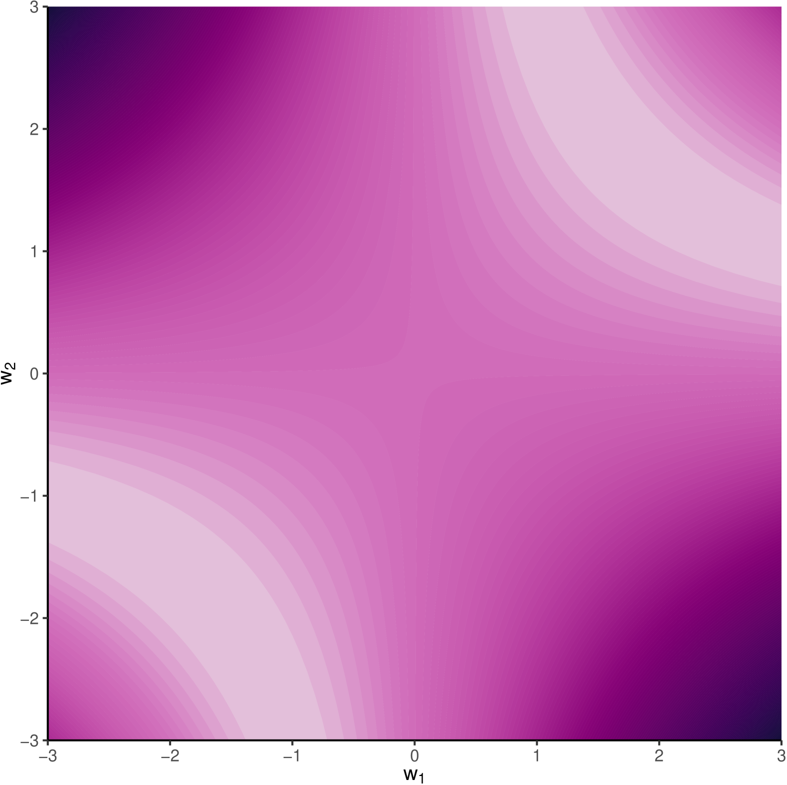
(a) $\eta=0$

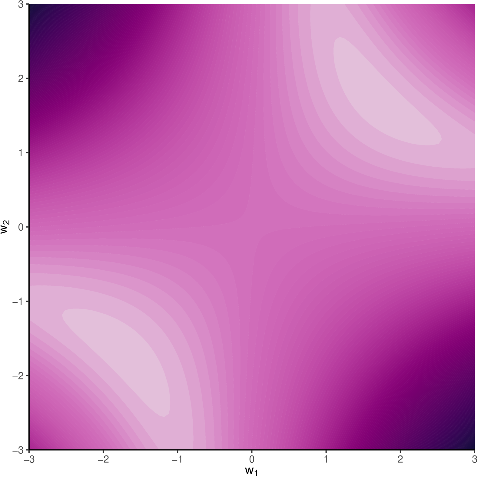
(b) $\eta=0.5$

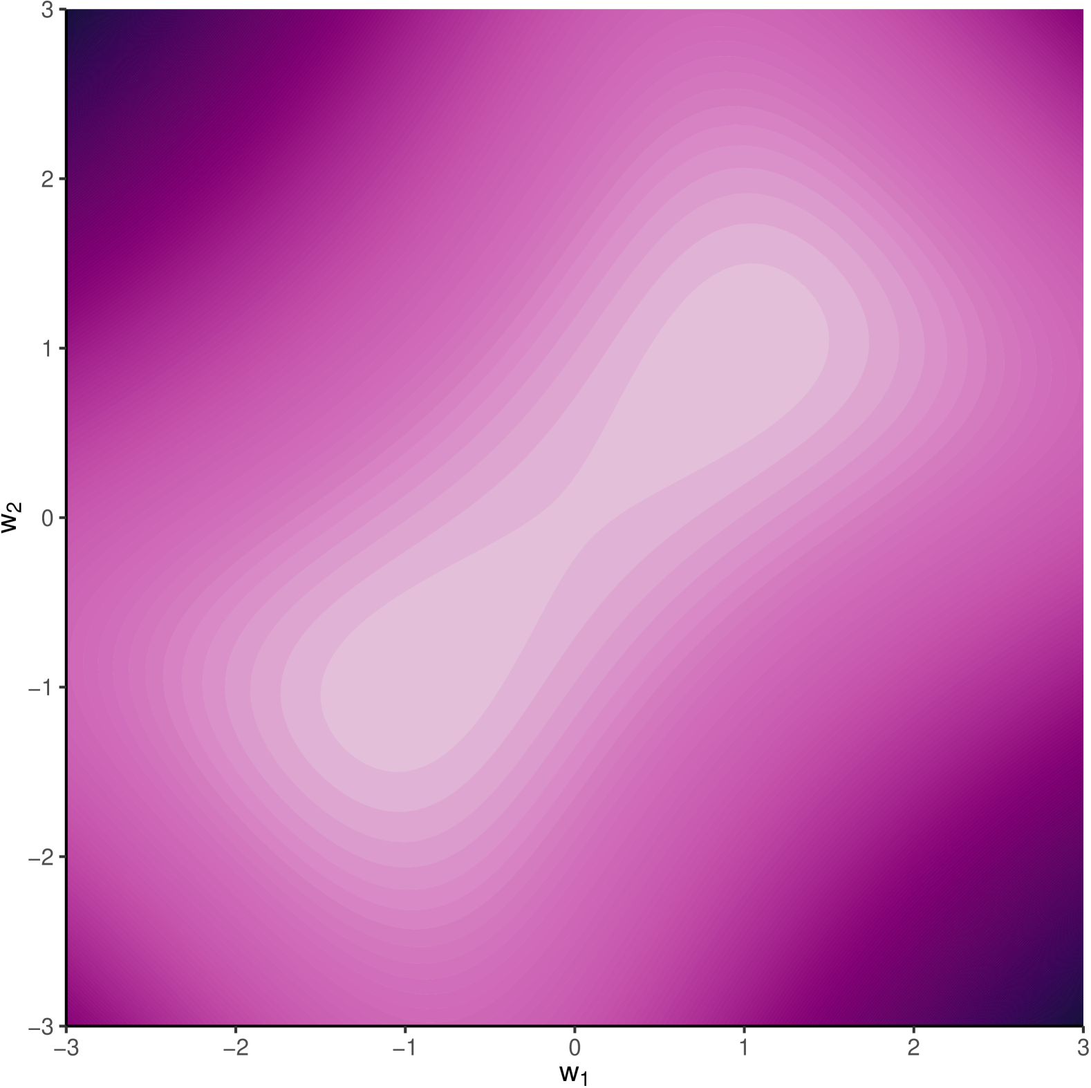
(c) $\eta=1.5$

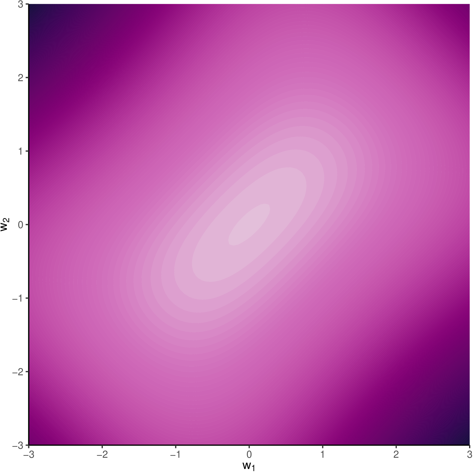
(d) $\eta=2$

Figure 2: Contour plots of the loss $(w_{*}-w_{2}w_{1})^{2}+\eta^{2}(w_{1}^{2}+w_{2}^{2})$ with $w_{*}=3.14159$ and different values of $\eta$. Large values of $\eta$ cause increasing shrinkage of the critical points towards zero.

For a well-chosen regularization parameter $\eta$, the addition of $R$ replaces the manifold of minimizers with two single points, lying close to the vertices of the hyperbola $(w_{*}-w_{2}w_{1})^{2}=0$. Intuitively, this is due to the quadratic penalty “locally coercifying” the loss. Along each level set of $\mathcal{L}$, the quadratic $R$ is minimized when $w_{2}^{2}=w_{1}^{2}$. Consequently, the global minimizers of $\mathcal{L}_{R}$ lie close to the intersection between $\operatorname*{arg\,min}\mathcal{L}$ and the constraint set $w_{2}^{2}-w_{1}^{2}=0$, subject to some additional shrinkage depending on the regularization strength $\eta^{2}$.

We now prove equivalents of these properties that generalize from the one-dimensional setting in the next theorem. Recall the convention that $\nabla_{W_{\ell}}\mathcal{L}$ and $\nabla_{W_{\ell}}R$ are themselves diagonal matrices, with the entries of the gradient vector as diagonal elements.

Theorem 3.1.

The function $\mathcal{L}_{R}$ of Lemma 2.2 satisfies the following:

1. The critical set of $\mathcal{L}_{R}$ is contained in the hyper-surface defined by the system of polynomial equations

   $$\nabla_{W_{\ell+1}}R(W)W_{\ell+1}=\nabla_{W_{\ell}}R(W)W_{\ell},\qquad\ell=1,\ldots,L-1.$$

   In particular, this entails $W_{\ell}^{2}=W_{m}^{2}$ for all $\ell\neq m$.

2. Every critical point $(W_{1},\ldots,W_{L})$ of $\mathcal{L}_{R}$ has the form

   $$W_{\ell,hh}=s_{\ell,h}\lambda_{h}\cdot\lvert W_{*}\rvert_{hh}^{1/L},$$ (13)

   where the signs $s_{1,h},\ldots,s_{L,h}\in\{-1,0,1\}$ either satisfy $s_{1,h}\cdots s_{L,h}=\mathrm{sign}(W_{*,hh})$, or $s_{1,h}=\cdots=s_{L,h}=0$. For $s_{1,h}\cdots s_{L,h}\neq 0$ the shrinkage factor $\lambda_{h}\in(0,1)$ is any positive root of

   $$0=\lambda_{h}^{2}-\lambda_{h}^{1-1/(L-1)}+\dfrac{\eta^{2}}{\lvert W_{*}\rvert_{hh}^{2/L}}.$$

   Moreover, $s_{1,h}\cdots s_{L,h}\neq 0$ is only possible if

   $$\lvert W_{*}\rvert_{hh}\geq\begin{cases}\eta^{2}&\mbox{for }L=2,\\ \left(\dfrac{L-2}{L}\right)^{L/2}\left(1+\dfrac{L}{L-2}\right)^{L-1}\cdot\eta^{L}&\mbox{otherwise.}\end{cases}$$ (14)

   in which case each $\lambda_{h}$ may take at most two distinct non-zero values, both satisfying

   $$\left(\dfrac{\eta^{2}}{\lvert W_{*}\rvert_{hh}^{2/L}}\right)^{(L-1)/(L-2)}\leq\lambda_{h}\leq\sqrt{1-\dfrac{\eta^{2}}{\lvert W_{*}\rvert_{hh}^{2/L}}}.$$

3. Fix a critical point $(W_{1},\ldots,W_{L})$ of $\mathcal{L}_{R}$ and let $\lambda_{h}$, $h=1,\ldots,d$ denote the corresponding shrinkage factors in (13), with the convention that $\lambda_{h}=0$ whenever $\mathrm{sign}(W_{\ell,hh})=0$, then

   $$\mathcal{L}_{R}\big{(}W_{1},\ldots,W_{L}\big{)}=\sum_{h=1}^{d}\Bigg{(}\Big{(}1-2\cdot\lambda_{h}^{L}\Big{)}\cdot\lvert W_{*}\rvert_{hh}^{2}+\bigg{(}\Big{(}\lambda_{h}\cdot\lvert W_{*}\rvert_{hh}^{1/L}\Big{)}^{2}+\eta^{2}\bigg{)}^{L}\Bigg{)}.$$

Theorem 3.1(a) generalizes the constraint set $w_{2}^{2}-w_{1}^{2}=0$ of the one-dimensional problem. In fact, the first part of Theorem 3.1(a) holds for any differentiable regularizer $R$ and a general linear network, in which case the critical points are constrained to lie within the hyper-surface $W_{\ell+1}^{\mathsf{t}}\nabla_{W_{\ell+1}}R(W_{1},\ldots,W_{L})=\nabla_{W_{\ell}}R(W_{1},\ldots,W_{L})W_{\ell}^{\mathsf{t}}$. The resulting constraint $W_{\ell}^{2}=W_{\ell+1}^{2}$ is however specific to the diagonal network and the regularizer $R$ computed in Lemma 2.2. This is an instance of the balancing condition, which reads $W_{\ell+1}^{\mathsf{t}}W_{\ell+1}=W_{\ell}W_{\ell}^{\mathsf{t}}$ for non-diagonal matrices and commonly appears in the analysis of deep linear networks [ACH18, Aro+19, Bah+21]. Consequently, the average sharpness penalty forces stationary points to be balanced and any optimization algorithm yielding stationary points must eventually become attracted to the set of balanced parameters.

Theorem 3.1(b) describes the critical points of $\mathcal{L}_{R}$ as resulting from a shrinkage-thresholding operator applied to the true parameter $W_{*}$. Such operators also appear in the study of other algorithmic regularization techniques, for example in dropout [SS22]. The threshold in (14) depends both on the noise level $\eta$ and the number of layers $L$. If the underlying signal $W_{*,hh}$ is too weak in comparison with $\eta^{L}$, any critical point will be forced towards $W_{\ell,hh}=0$. Hence, the regularizer $R$ induces an explicit bias towards low-rank product matrices $W_{L}\cdots W_{1}$, with larger $\eta$ corresponding to lower ranks by truncating the smaller entries of $W_{*}$. This also describes the “coercification” of $\mathcal{L}$ through $R$, as regulated by $\eta$, see the change in landscape in Figure 2 for a depiction in the one-dimensional model. As $\eta$ increases, the non-zero critical points are gradually forced towards $0$, eventually merging into a single critical point at $0$, once $\lvert W_{*}\rvert_{hh}$ lies below the threshold. When $L\to\infty$, the right-hand side of (14) approximates $2^{L-1}\cdot\eta^{L}$, asymptotically requiring $\eta=O(2^{-1+1/L})$ to allow for a non-zero solution. In this case, the equation solved by the non-zero shrinkage factors converges to the quadratic equation $0=\lambda_{h}^{2}-\lambda_{h}+\eta^{2}$.

Together, Theorem 3.1(a) and 3.1(b) illustrate how the regularizer $R$ controls the parameter norm near stationary points of $\mathcal{L}_{R}$. As in the one-dimensional case, $\lambda_{\ell}\cdot W_{\ell}$ with any scalars $\lambda_{1}\cdots\lambda_{L}=1$ factorizes $W=W_{L}\cdots W_{1}$. Taking $\lambda_{1}\to\infty$, while sending the other scalars to zero at a matching rate, then gives a factorization of $W$ with arbitrarily large parameter norm. Forcing the weight matrices to be approximately balanced near the stationary set rules out this escape to infinity. A quantitative relation between parameter norm and balancing is given in Proposition 3.2 of [NRT24].

As shown in Theorem 3.1(c), the regularizer induced by S-SAM prevents the optimization algorithm from reaching zero loss on the original empirical landscape. The loss $\mathcal{L}$ admits its minimal value $0$ for any $W_{L}\cdots W_{1}=W_{*}$. Conversely, $R$ always reaches its minimal value when $W_{L}=\cdots=W_{1}=0$. Trading off between the two criteria induces shrinkage, much in the same way as the squared norm penalty does in ridge regression (Chapter 3.4.1 in [HTF09]). Unlike the ridge regression model, the non-convex loss $\mathcal{L}_{R}$ admits many critical points, with differing fits to the underlying parameter $W_{*}$. This fundamentally distinguishes factorized models from the convex linear regression model.

We conclude our study of the regularized landscape $\mathcal{L}_{R}$ by directly relating the balancing constraint in Theorem 3.1(a) to the average sharpness $S_{\mathrm{avg}}$ and the trace of the Hessian matrix, proving that the balancing explicitly controls both of the latter.

Lemma 3.2.

Fix a $(d\times d)$-diagonal matrix $W$ and define $\pi(W)=\{W_{1},\ldots W_{L}\mid W=W_{L}\cdots W_{1}\}$, with each $W_{\ell}$ also diagonal, then

$$\big{(}W_{1},\ldots,W_{L}\big{)} \mapsto S_{\mathrm{avg}}\big{(}W_{L}\cdots W_{1},\eta\big{)}$$

$$\big{(}W_{1},\ldots,W_{L}\big{)} \mapsto\mathrm{Tr}\Big{(}\nabla^{2}\mathcal{L}\big{(}W_{L}\cdots W_{1}\big{)}\Big{)}$$

attain their minima over $\pi(W)$ if, and only if, $W_{\ell}^{2}=W^{2}_{\ell+1}$ for every $\ell=1,\ldots,L-1$.

Recall from the discussion surrounding Lemma 2.3 that average sharpness and parameter norm together act as a generalization measure for linear neural networks training on the squared Euclidean loss $\mathcal{L}$. Combining Theorem 3.1 and Lemma 3.2 proves that in the diagonal linear model the balancing constraint effectively controls both relevant quantities. Further, this constraint decreases the model complexity by reducing the effective number of parameters.

4 Convergence of the S-SAM Recursion

Having characterized the change in landscape induced by the average sharpness regularizer, we now prove that the S-SAM recursion (6) indeed produces a critical point of the expected loss $\mathcal{L}_{R}$. Our analysis is inspired by techniques found in [Bah+21], [Cha22], and [NRT24]. For simplicity, we consider solely the case of diagonal weight matrices. Crucially, the presence of the regularizer $R$ allows us to simplify certain arguments relating to the boundedness of the trajectories.

4.1 Gradient Flow Analysis

For each $\ell=1,\ldots,L$, the weight matrices $W_{\ell}=W_{\ell}(t)$, $t\geq 0$, are said to follow the gradient flow of $\mathcal{L}_{R}$ if they solve the system of ordinary differential equations (12) with given boundary conditions $W_{1}(0),\ldots,W_{L}(0)$, meaning they evolve along the negative of the gradient vector field of $\mathcal{L}_{R}$. Existence and uniqueness of the gradient flow trajectories follows from standard theorems on ordinary differential equations, see for example Chapter 2 of [Tes12]. The continuous time index $t\in[0,\infty)$ may be interpreted as the limit of vanishing step-sizes in the corresponding gradient descent recursion generated by $\mathcal{L}_{R}$. We wish to invert this relation; we first prove a result for the gradient flows and then generalize it to discrete time.

As a consequence of the definition, the loss $\mathcal{L}_{R}$ may never increase in $t$, provided that each weight matrix $W_{\ell}$ follows the gradient flow of $\mathcal{L}_{R}$. Indeed, since the time derivative of each $W_{\ell}(t)$, $\ell=1,\ldots,L$ equals the respective negative gradient of $\mathcal{L}_{R}$, the chain rule implies

$$\dfrac{\mathrm{d}}{\mathrm{d}t}\mathcal{L}_{R}\big{(}W_{1}(t),\ldots,W_{L}(t)\big{)} =\sum_{\ell=1}^{L}\left\langle\nabla_{W_{\ell}}\mathcal{L}_{R}\big{(}W_{1}(t),\ldots,W_{L}(t)\big{)},\dfrac{\mathrm{d}}{\mathrm{d}t}W_{\ell}(t)\right\rangle$$

$$=-\sum_{\ell=1}^{L}\big{\lVert}\nabla_{W_{\ell}}\mathcal{L}_{R}\big{(}W_{1}(t),\ldots,W_{L}(t)\big{)}\big{\rVert}^{2},$$ (15)

so the derivative of $\mathcal{L}_{R}$ stays non-positive along the whole trajectory. We will now show that this already implies convergence to a critical point of $\mathcal{L}_{R}$ as $t\to\infty$.

Łojasiewicz’s Theorem on gradient flows [Łoj84], restated in Appendix D, shows that the gradient flow of any analytic function either diverges to infinity, or yields a critical point of said function. If the trajectories of $W_{\ell}(t)$ in (12) stay bounded, they must then necessarily converge to a critical point of $\mathcal{L}_{R}$ as $t\to\infty$. Ensuring boundedness of the trajectories may in general contain the bulk of the difficulty, see for example the proof of Theorem 3.2 in [Bah+21], but we can profitably employ the regularizer $R$. Combining non-negativity of $\mathcal{L}$ and $R$ with (8),

$$\sum_{\ell=1}^{L}\lVert W_{\ell}\rVert^{2}\leq\dfrac{1}{\eta^{2(L-1)}}\cdot R\big{(}W_{1},\ldots,W_{L}\big{)}\leq\dfrac{1}{\eta^{2(L-1)}}\cdot\mathcal{L}_{R}\big{(}W_{1},\ldots,W_{L}\big{)},$$

making the loss function $\mathcal{L}_{R}$ coercive. In particular, this bound holds along the entire trajectory of the gradient flow, so together with (15) we arrive at the estimate

$$\dfrac{1}{\eta^{L-1}}\cdot\sqrt{\mathcal{L}_{R}\big{(}W_{1}(0),\ldots,W_{L}(0)\big{)}}\geq\sqrt{\sum_{\ell=1}^{L}\lVert W_{\ell}(t)\rVert^{2}},$$ (16)

valid for all $t\geq 0$. The right-hand side of (16) denotes the Euclidean norm of the network parameter $(W_{1},\ldots,W_{L})$ as a vector in $\mathbb{R}^{Ld}$, so Łojasiewicz’s Theorem D.1 ensures the existence of $W_{\ell}(\infty)=\lim_{t\to\infty}W_{\ell}(t)$ for every $\ell$, which must be a critical point of $\mathcal{L}_{R}$.

Further, since $\mathcal{L}_{R}$ is locally Lipschitz continuous, we can integrate and rearrange (15) to show that the average norm of the gradient of $\mathcal{L}_{R}$ along the gradient flow trajectory vanishes at a linear rate in time

$$\dfrac{1}{t}\cdot\int_{0}^{t}\sum_{\ell=1}^{L}\big{\lVert}\nabla_{W_{\ell}}\mathcal{L}_{R}\big{(}W_{1}(s),\ldots,W_{L}(s)\big{)}\big{\rVert}^{2}\ \mathrm{d}s =\dfrac{1}{t}\cdot\Big{(}\mathcal{L}_{R}\big{(}W_{1}(0),\ldots,W_{L}(0)\big{)}-\mathcal{L}_{R}\big{(}W_{1}(t),\ldots,W_{L}(t)\big{)}\Big{)}$$

$$\leq\dfrac{1}{t}\cdot\mathcal{L}_{R}\big{(}W_{1}(0),\ldots,W_{L}(0)\big{)}.$$ (17)

The arguments employed so far work for any analytic loss function that is coercive, in the sense that it upper-bounds a suitable transformation of the parameter norm. In our case, this transformation happens to be the quadratic monomial (8).

Exploiting the specific structure of the loss $\mathcal{L}_{R}$, we are moreover able to give a quantitative version of the constraint in Theorem 3.1(a) along the trajectory of the gradient flow.

Theorem 4.1.

For every $\ell=1,\ldots,L$ and all $t\geq 0$,

$$\big{\lVert}W_{\ell}^{2}(t)-W_{\ell+1}^{2}(t)\big{\rVert}\leq\exp\Big{(}-4\eta^{2L-2}\cdot t\Big{)}\cdot\big{\lVert}W_{\ell}^{2}(0)-W_{\ell+1}^{2}(0)\big{\rVert}.$$

As mentioned in the discussion following Theorem 3.1, the balancing constraint $W_{\ell}^{2}-W_{\ell+1}^{2}$ plays an instrumental role in controlling the parameter norm at the critical points of $\mathcal{L}_{R}$. Based on Theorem 4.1, we conclude that the regularizer $R$ not only provides this control asymptotically by changing the landscape at the stationary points, but also forces the gradient flow of $\mathcal{L}_{R}$ to rapidly balance the weight matrices. This stands in stark contrast with the gradient flow of the unregularized objective $\mathcal{L}$, for which the balancing remains unchanged along its trajectories [ACH18, Bah+21]. Combining Lemma 3.2 with Theorem 4.1 also proves that the gradient flow minimizes the average sharpness $S_{\mathrm{avg}}$ and the trace of the Hessian matrix at an exponential rate along its trajectory.

4.2 Generalizing to Gradient Descent

The convergence result for gradient flows presented in Section 4.1 exploits the basic monotonicity property (15), which is inherent to the definition of gradient flows. Due to discretization error, the argument does not extend to discrete time without some preparation. As illustrated in [Cha22], or the extension of Theorem 2.3 of [Bah+21] on gradient flows to gradient descent in Theorem 2.4 of [NRT24], the discretization must be chosen carefully.

For a sequence of positive step-sizes $\alpha_{k}$ and initial values $W_{1}(0),\ldots,W_{L}(0)$, the discrete-time analog of (12) is given by the gradient descent recursions

$$W_{\ell}(k+1)=W_{\ell}(k)-\alpha_{k}\cdot\nabla_{W_{\ell}(k)}\mathcal{L}_{R}\big{(}W_{1}(k),\ldots,W_{L}(k)\big{)}.$$ (18)

We aim to apply the generic Łojasiewicz-type theorem for discrete-time iterations shown in [AMA05]. See Theorem D.3 for a restatement and subsequently Lemma D.4 for a version adapted to gradient descent. Analogous to the result for gradient flows, the theorem states that the gradient descent iterates of analytic functions either diverge to infinity or converge to a critical point of the function, given regularity conditions. The sole requirement for this result is the so-called strong descent condition. In our notation, the condition may be stated as the existence of $\delta>0$, such that

$$\mathcal{L}_{R}\big{(}W_{1}(k),\ldots,W_{L}(k)\big{)}-\mathcal{L}_{R}\big{(}W_{1}(k+1),\ldots,W_{L}(k+1)\big{)}\geq\delta\alpha_{k}\cdot\sum_{\ell=1}^{L}\big{\lVert}\nabla_{W_{\ell}(k)}\mathcal{L}_{R}\big{(}W_{1}(k),\ldots,W_{L}(k)\big{)}\big{\rVert}^{2}$$ (19)

for every $k\geq 0$. This ensures a monotonically decreasing loss along the trajectory of the gradient descent (18), giving a discrete-time equivalent of (15). For loss functions with globally Lipschitz continuous gradients, it suffices that $\alpha_{k}$ never exceeds twice the reciprocal of the Lipschitz constant [GG24]. When $L>1$, the loss $\mathcal{L}_{R}$ is polynomial in the weights $W_{\ell,ii}$ with leading terms of the form $W_{L,ii}^{2}\cdots W_{1,ii}^{2}$. Consequently, $\nabla\mathcal{L}_{R}$ only admits local Lipschitz continuity and verifying (19) along the gradient descent trajectory requires a careful account of local Lipschitz constants. If the strong descent condition can be proven for every $k$, then the bound (16) holds with the continuous-time index $t$ replaced by $k$, implying boundedness of the whole trajectory. This is the main idea behind the next theorem.

Theorem 4.2.

Consider the diagonal linear model, fix $\delta\in(0,1)$, and let $W_{\ell}(k)$, $\ell=1,\ldots,L$ be generated by the gradient descent recursion (18), with step-sizes $\alpha_{k}$ satisfying $\sum_{k=0}^{\infty}\alpha_{k}=\infty$ and

$$\sup_{k\geq 0}\alpha_{k}<2(1-\delta)\cdot\left(\sqrt{L}\cdot\dfrac{7\sqrt{L}+2}{\eta^{2}}\cdot\mathcal{L}_{R}\big{(}W_{1}(0),\ldots,W_{L}(0)\big{)}\right)^{-1}.$$

Then, the strong descent condition (19) holds with the chosen $\delta$ for every $k\geq 0$. Consequently, the discrete-time analog of the upper-bound (16) is satisfied for every $k\geq 0$ and the gradient descent iterates converge to a critical point of $\mathcal{L}_{R}$ as $k\to\infty$.

We briefly comment on the role of the step-sizes in the proof of the previous theorem. By definition, $W_{\ell}(k+1)-W_{\ell}(k)=-\alpha_{k}\cdot\nabla_{W_{\ell}(k)}\mathcal{L}_{R}\big{(}W_{1}(k),\ldots,W_{L}(k)\big{)}$ and so a first-order expansion of $\mathcal{L}_{R}$ around $W_{1}(k),\ldots,W_{L}(k)$ leads to

$$\mathcal{L}_{R}\big{(}W_{1}(k+1),\ldots,W_{L}(k+1)\big{)}-\mathcal{L}_{R}\big{(}W_{1}(k),\ldots,W_{L}(k)\big{)}$$

$$=\ \sum_{\ell=1}^{L}\Big{\langle}\nabla_{W_{\ell}(k)}\mathcal{L}_{R}\big{(}W_{1}(k),\ldots,W_{L}(k)\big{)},W_{\ell}(k+1)-W_{\ell}(k)\Big{\rangle}+O\left(\sum_{\ell=1}^{L}\big{\lVert}W_{\ell}(k+1)-W_{\ell}(k)\big{\rVert}^{2}\right)$$

$$= -\alpha_{k}\cdot\sum_{\ell=1}^{L}\big{\lVert}\nabla_{W_{\ell}(k)}\mathcal{L}_{R}\big{(}W_{1}(k),\ldots,W_{L}(k)\big{)}\big{\rVert}^{2}+O\left(\alpha_{k}^{2}\cdot\sum_{\ell=1}^{L}\big{\lVert}\nabla_{W_{\ell}(k)}\mathcal{L}_{R}\big{(}W_{1}(k),\ldots,W_{L}(k)\big{)}\big{\rVert}^{2}\right).$$ (20)

If the quadratic approximation error in (20) can be controlled in a uniform manner via suitable selection of the step-sizes, then the latter may be rearranged to exhibit the strong descent conditions (19) with the chosen $\delta$. The assumption on $\sup_{k}\alpha_{k}$ in Theorem 4.2 ensures that the local Lipschitz constants of $\nabla\mathcal{L}_{R}$ along the gradient descent trajectory remain under uniform control, giving the desired bound.

The bulk of the difficulty in proving Theorem 4.2 lies in finding an efficient estimate for the operator norm of $\nabla^{2}\mathcal{L}_{R}$. As shown in Lemma 2.2, the regularizer $R$ is defined in terms of a product over matrices $W_{\ell}^{2}+\eta^{2}\cdot I_{d}$. Expanding this product and individually bounding the second derivatives of each term would yield a bound for $\nabla^{2}\mathcal{L}_{R}$ of the order $O(2^{L}\cdot\mathcal{L}_{R}(W_{1}(0),\ldots,W_{L}(0))^{L})$. Since the maximal step-size $\sup_{k}\alpha_{k}$ must lie below twice the reciprocal of the estimated operator norm, this would lead to slow convergence for even moderately large $L$ and bad initializations. By exploiting the specific form (7) of the regularizer $R$, one can improve this estimate to $O\big{(}L\cdot\mathcal{L}_{R}(W_{1}(0),\ldots,W_{L}(0))\big{)}$, as shown in the assumption on $\sup\alpha_{k}$ in Theorem 4.2. In comparison, the corresponding operator norm estimate for the unregularized descent scales like $O(L^{2L}\cdot\mathcal{L}_{R}(W_{1}(0),\ldots,W_{L}(0))^{2})$, unless the initial matrices are chosen close to being balanced. See Theorem 2.4 and Remark 2.5 in [NRT24] for further details.

For constant step-sizes $\alpha_{k}=\alpha$ satisfying the requirements of Theorem 4.2, summing over (19) yields the discrete-time equivalent of the convergence rate 17, namely

$$\dfrac{\delta\alpha}{k}\cdot\sum_{j=0}^{k-1}\sum_{\ell=1}^{L}\big{\lVert}\nabla_{W_{\ell}(j)}\mathcal{L}_{R}\big{(}W_{1}(j),\ldots,W_{L}(j)\big{)}\big{\rVert}^{2}\leq\dfrac{1}{k}\cdot\mathcal{L}_{R}\big{(}W_{1}(0),\ldots,W_{L}(0)\big{)}.$$

To conclude our analysis of (18), we prove a discrete-time version of Theorem 4.1. Consequently, the addition of the regularizer $R$ changes the gradient descent dynamics in a manner similar to the gradient flow, forcing balancing of the weight matrices. As mentioned following Theorem 4.1, this controls the generalization measures shown in Lemma 2.3.

Theorem 4.3.

In addition to the assumptions of Theorem 4.2, suppose

$$\sup_{k\geq 0}\alpha_{k}<\min\ \left\{\dfrac{1}{\eta^{2L-2}},\ \dfrac{\eta^{2}}{4\mathcal{L}_{R}\big{(}W_{1}(0),\ldots,W_{L}(0)\big{)}},\ \dfrac{3\eta^{2L+2}}{16\big{(}1+\lVert W_{*}\rVert\big{)}}\min\ \bigg{\{}1,\ \mathcal{L}_{R}\big{(}W_{1}(0),\ldots,W_{L}(0)\big{)}^{-2}\bigg{\}}\right\}.$$

Then, for every $k\geq 0$ and every $\ell=1,\ldots,L-1$

$$\big{\lVert}W_{\ell}^{2}(k)-W_{\ell+1}^{2}(k)\big{\rVert}\leq\left(\prod_{j=0}^{k-1}\big{(}1-\alpha_{j}\eta^{2L-2}\big{)}\right)\cdot\big{\lVert}W_{\ell}^{2}(0)-W_{\ell+1}^{2}(0)\big{\rVert}.$$

For a depiction of Theorem 4.3 in action, see Figure 3. Once the unregularized gradient descent (4) reaches a critical point of $\mathcal{L}$, the algorithm naturally terminates. In contrast, the regularizer $R$ continually forces the iterates (18) towards a balanced solution, with larger values of $\eta$ corresponding to faster balancing. The speed of convergence in Theorem 4.3 also depends on the step-sizes $\alpha_{k}$, with a constant step-size $\alpha_{k}=\alpha$ giving a geometric rate. Choosing $\alpha_{k}=\alpha/(k+1)$ for some suitable constant $\alpha>0$ leads to balancing at the rate $k^{-\alpha\eta^{2L-2}}$. Indeed, since $\log(1-x)\approx-x$ for small enough $x\in(0,1)$,

$$\prod_{j=0}^{k-1}\big{(}1-\alpha_{j}\eta^{2L-2}\big{)}=\exp\left(\sum_{j=0}^{k-1}\log\big{(}1-\alpha_{j}\eta^{2L-2}\big{)}\right)\approx\exp\left(-\alpha\eta^{2L-2}\cdot\sum_{j=1}^{k}\dfrac{1}{j}\right)$$

and the rate now follows from $\sum_{j=1}^{k}j^{-1}\approx\log(k)$.

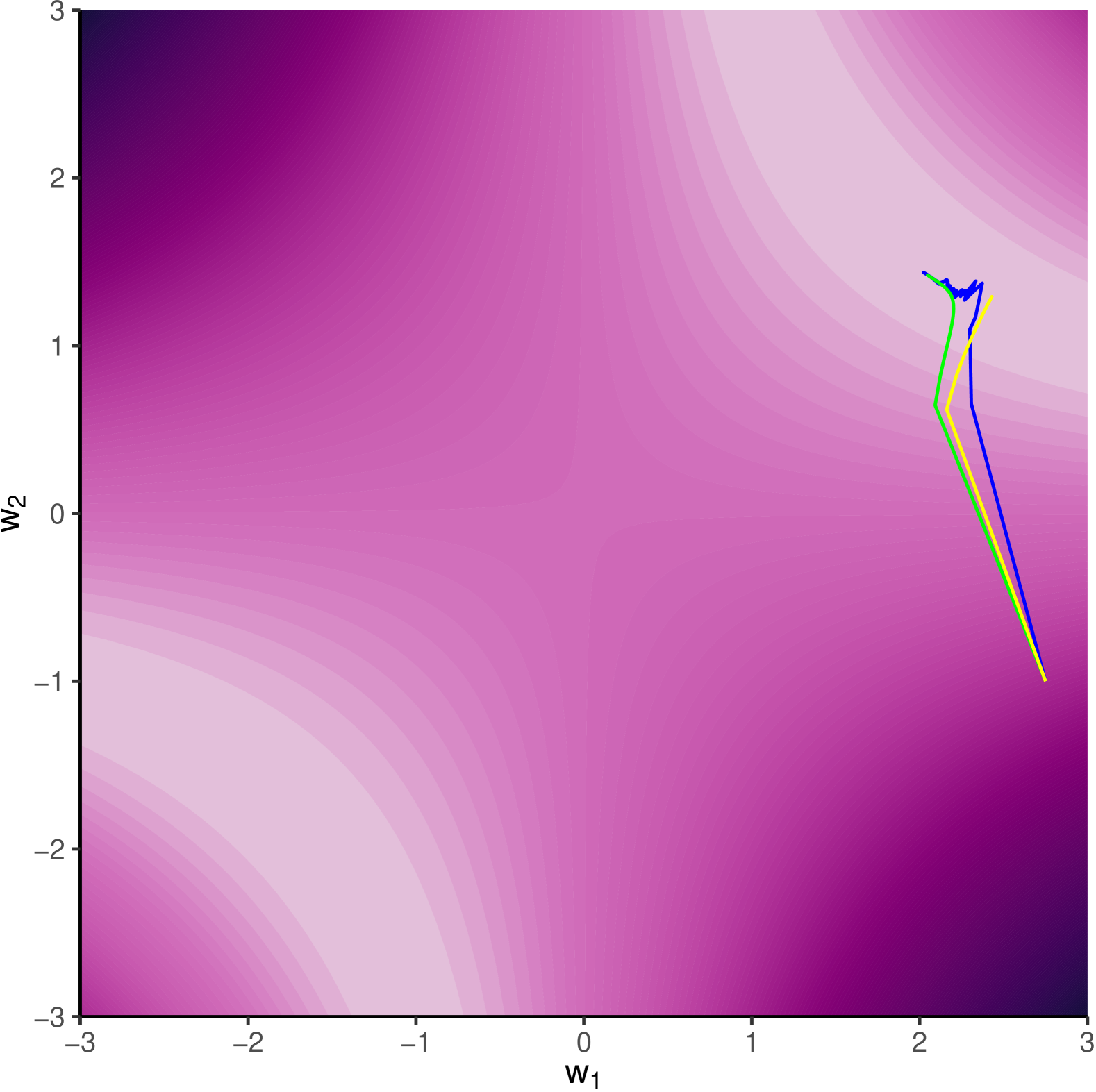
(a) $\eta=0.5$ and $\alpha_{k}=0.1/(k+1)$

(b) $\eta=1$ and $\alpha_{k}=0.1/(k+1)$

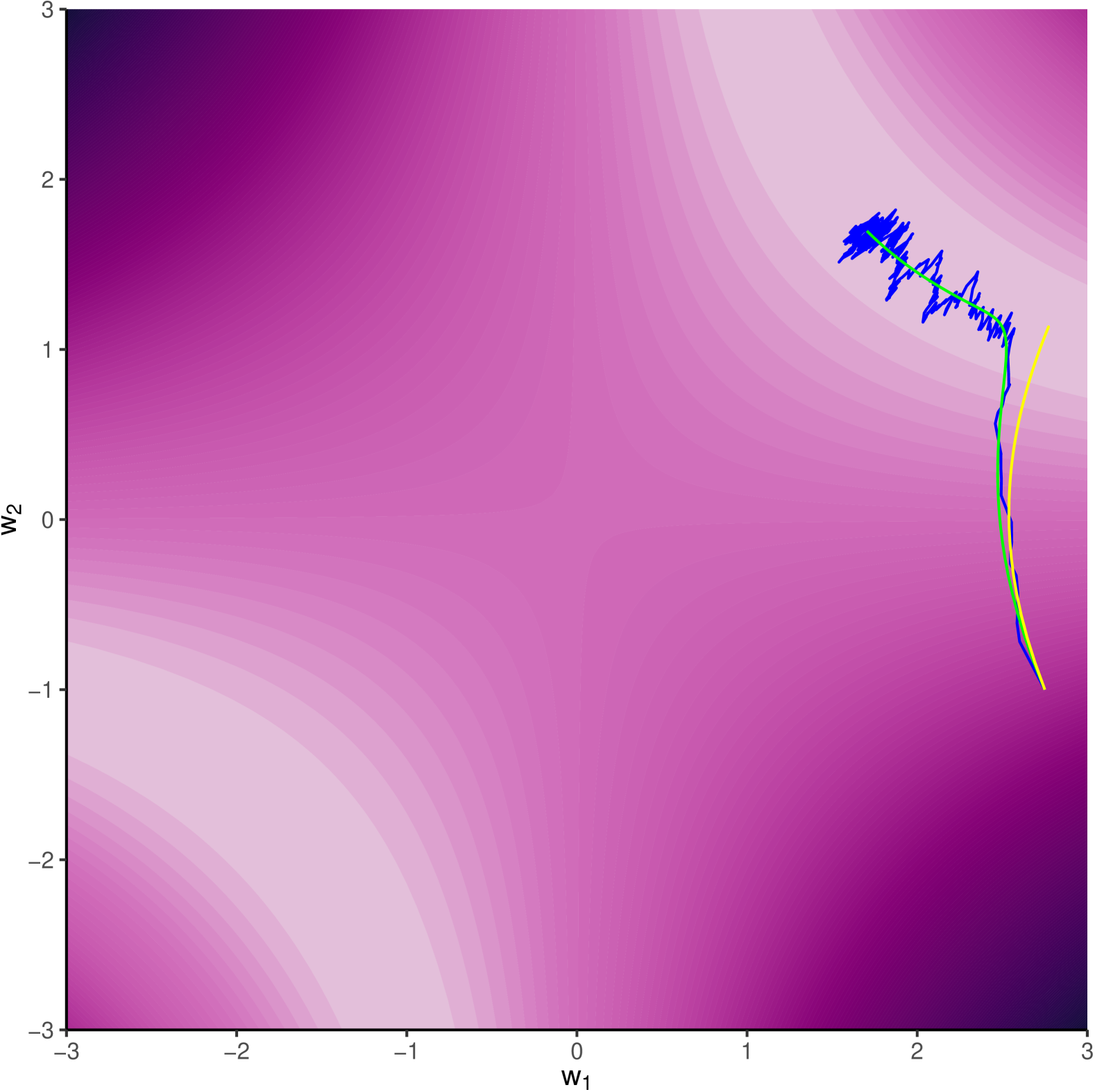
(c) $\eta=0.5$ and $\alpha_{k}=0.01$

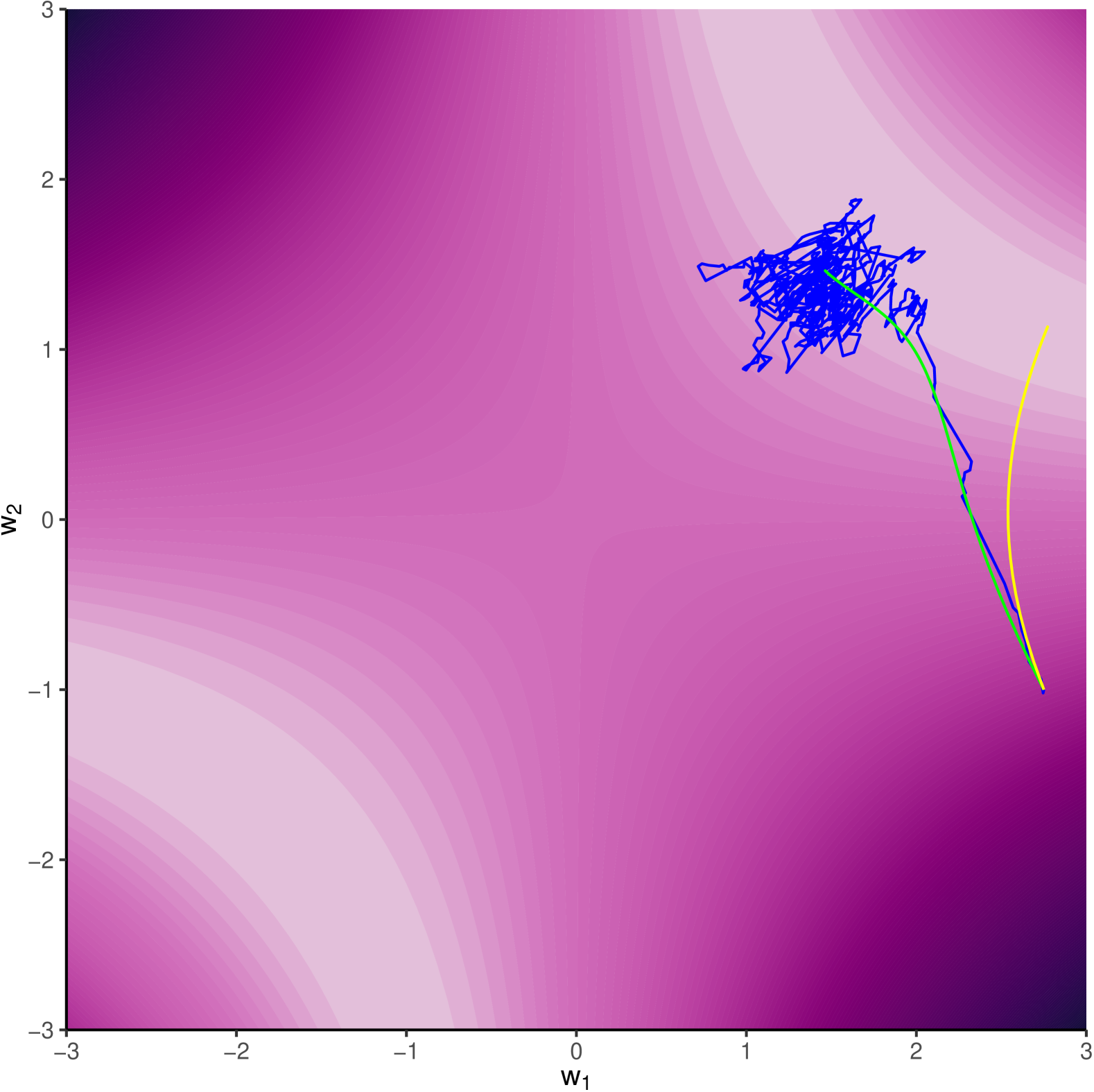
(d) $\eta=1$ and $\alpha_{k}=0.01$

Figure 3: Gradient descent trajectories overlaid onto a contour plot of the loss $(w_{*}-w_{2}w_{1})^{2}$ with $w_{*}=3.14159$, started from the same initial point and run with different values of $\eta$ and $\alpha_{k}$. Shown are standard gradient descent following $-\nabla\mathcal{L}$ (yellow), explicitly regularized gradient descent following $-\nabla\mathcal{L}_{R}$ (green), and gradient descent with S-SAM following $-\nabla\widetilde{\mathcal{L}}_{k}$ (blue).

4.3 Convergence of the Projected Stochastic Recursion

On the event that the iterates stay bounded, almost sure convergence towards a root of the expected gradient can be ensured for a large class of functions [Dav+20, DK24], provided the step-sizes $\alpha_{k}$ adequately control the variance of the gradient noise. To ensure boundedness, we will consider a version of the S-SAM recursion (6) projected onto a compact set.

Recall from Section 2 that we are given a supervised sample $(\mathbf{X}_{i},Y_{i})$, $i=1,\ldots,n$ with $Y_{i}=\mathbf{1}^{\mathsf{t}}W_{*}\mathbf{X}_{i}$, where $\mathbf{1}$ denotes the vector with every entry equaling $1$. Suppose $(\mathbf{X},Y)\sim\mathrm{Unif}\big{(}(\mathbf{X}_{1},Y_{1}),\ldots,(\mathbf{X}_{n},Y_{n})\big{)}$ and $\bm{\xi}\sim\mathcal{N}(0,\eta^{2}\cdot I_{Ld})$, then the S-SAM recursion (6) moves during every iteration along the negative gradient of an independent sample from the random function

$$\widetilde{\mathcal{L}}\big{(}W_{1},\ldots,W_{L}\big{)}=\left(Y-\sum_{j=1}^{d}\Big{(}\widetilde{W}_{L}\cdots\widetilde{W}_{1}\mathbf{X}\Big{)}_{j}\right)^{2},$$ (21)

with $\widetilde{W}_{\ell,ii}=W_{\ell,ii}+\xi_{\ell,ii}$. To take an independent sample $\widetilde{\mathcal{L}}_{k}\sim\widetilde{\mathcal{L}}$ of this randomized loss, we may independently sample $\bm{\xi}_{k}\sim\bm{\xi}$ and $\mathbf{X}_{k}\sim\mathbf{X}$ and simply plug in the outcomes. As shown in Lemma 2.2, the dynamical system generated by $-\nabla\widetilde{\mathcal{L}}_{k}$, with an independent sample $\widetilde{\mathcal{L}}_{k}$ taken during every time-step, may be decomposed into $-\nabla\mathcal{L}_{R}+\zeta_{k}$ with $\zeta_{k}=\nabla\mathcal{L}_{R}-\nabla\widetilde{\mathcal{L}}_{k}$ forming a martingale difference sequence. The random vector $\bm{\xi}$ has unbounded support and so $\sup_{k\geq 0}\lVert\nabla\widetilde{\mathcal{L}}_{k}\rVert=\infty$. To ensure that the algorithm produces almost surely bounded trajectories, we focus on the case where the weights are projected onto a compact set after every iteration. This makes the algorithm amenable to a convergence result in [Dav+20]. Given $r>0$, let $\Pi_{r}$ denote the projection onto the Euclidean ball of radius $r$ in $\mathbb{R}^{Ld}$. Applied to the weight matrices $(W_{1},\ldots,W_{L})$, this gives

$$\Pi_{r}\left(\begin{bmatrix}W_{1}\\ \vdots\\ W_{L}\end{bmatrix}\right)=\min\left\{1,\ \dfrac{r}{\sqrt{\sum_{\ell=1}^{L}\lVert W_{\ell}\rVert^{2}}}\right\}\cdot\begin{bmatrix}W_{1}\\ \vdots\\ W_{L}\end{bmatrix}$$

and the projected S-SAM iterates take the form

$$\begin{bmatrix}W_{1}(k+1)\\ \vdots\\ W_{L}(k+1)\end{bmatrix}=\Pi_{r}\left(\begin{bmatrix}W_{1}(k)\\ \vdots\\ W_{L}(k)\end{bmatrix}-\alpha_{k}\cdot\begin{bmatrix}\nabla_{W_{1}(k)}\widetilde{\mathcal{L}}_{k}\big{(}W_{1}(k),\ldots,W_{L}(k)\big{)}\\ \vdots\\ \nabla_{W_{1}(k)}\widetilde{\mathcal{L}}_{k}\big{(}W_{1}(k),\ldots,W_{L}(k)\big{)}\end{bmatrix}\right).$$ (22)

By definition, the resulting trajectories always stay confined to the ball of radius $r$ and every limit point of the iterates must then be a critical point of $\mathcal{L}_{R}$.

Theorem 4.4.

Suppose the step-sizes $\alpha_{k}$ satisfy $\sum_{j=0}^{\infty}\alpha_{j}=\infty$ and $\sum_{j=0}^{\infty}\alpha_{j}^{2}<\infty$. Pick a radius $r$ such that

$$r\geq\max\left\{1,\ \dfrac{\sqrt{L}}{2\eta^{L-1}}\right\}\cdot\lVert W_{*}\rVert$$

Then, every limit point of the projected S-SAM recursion (22) is a critical point of $\mathcal{L}_{R}$ and the function values $\mathcal{L}_{R}\big{(}W_{1}(k),\ldots,W_{L}(k)\big{)}$ converge as $k\to\infty$.

The assumption on the step-sizes $\alpha_{k}$ in Theorem 4.4 is standard in the stochastic approximation literature and known as the Robbins-Monro condition after [RM51]. Since $-\alpha_{k}\cdot\nabla\widetilde{\mathcal{L}}_{k}=-\alpha_{k}\cdot\nabla\mathcal{L}_{R}+\alpha_{k}\cdot\zeta_{k}$, the variance of the random gradients may be controlled by $\alpha_{k}^{2}\cdot\mathbb{E}\big{[}\lVert\zeta_{k}\rVert^{2}\big{]}$, so picking square summable step-sizes ensures that the random gradients converge to their expectations in squared mean at a sufficiently fast rate.

The condition on the radius $r$ rules out cases where the iterates asymptotically stick to the boundary of the ball. For smaller radii, the vector field $-\nabla\mathcal{L}_{R}$ may pull the iterates towards a stationary point outside the ball of radius $r$. Since the regularized loss $\mathcal{L}_{R}$ is roughly quadratic at large scales by (8), we may pick $r$ large enough so that all critical points have norm strictly less than $r$ and the vector field $-\nabla\mathcal{L}_{R}$ always transports the iterates back into the ball at the boundary. The lower-bound on $r$ in Theorem 4.4 depends on the norm of $W_{*}$, which is known in our diagonal linear network model due to the assumed invertibility of $n^{-1}\cdot\sum_{i=1}^{n}\mathbf{X}_{i}\mathbf{X}_{i}^{\mathsf{t}}$, see the beginning of Section 2. For more complex settings, the true parameter norm is unknown in practice and must be estimated from the data.

5 Conclusion and Outlook

We may summarize our results for S-SAM as follows: For diagonal linear networks, S-SAM induces balanced solutions, both by changing the expected loss landscape (Theorem 3.1(a)) and forcing the underlying gradient flow/descent dynamics to balance the weight matrices at a fast rate (Theorem 4.1 and Theorem 4.3). The balancing explicitly controls the sharpness (Lemma 3.2), so this also gives a rate at which the underlying dynamics minimize sharpness. Further, the induced regularizer controls the parameter norm of the gradient descent iterates by forcing them towards a shrinkage-thresholding of the true parameter (Theorem 3.1(a) and Theorem 4.2). Together, the parameter norm and sharpness measure the generalization performance (Lemma 2.3). Lastly, convergence towards a critical point can be shown for the projected gradient descent with S-SAM (Theorem D.5). We conclude that S-SAM has the intended effect in the diagonal linear setup and efficiently regularizes the algorithm to control the relevant generalization measures.

To complete the article, we now outline some possible directions for further research. A natural follow-up question concerns the behavior of S-SAM as a diffusion in the parameter space for constant step-sizes. Strong results in this vein exist for stochastic gradient Langevin dynamics (SGLD) [RRT17]. Unlike for SGLD, the gradient noise induced by S-SAM highly depends on the current parameter location. Characterizing the stationary distribution of gradient descent with some types of location-dependent noise is possible, but requires a finely tuned setup [YNI24]. In general, given sufficient regularity conditions, stochastic gradient descent with a constant step-size will converge to a stationary distribution that reflects the local geometry of the loss surface [Azi+24]. This is also illustrated in the constant step-size S-SAM trajectories shown in Figure 3, where the S-SAM gradient slowly minimizes the balancing of the weight matrices and then enters a stationary regime, concentrating around one of the global minimzers of $\mathcal{L}_{R}$. Unlike the explicitly regularized $\nabla\mathcal{L}_{R}$, the S-SAM algorithm does not necessarily decrease the balancing during every iteration. Rather, the balancing experiences a downward trend, due to the alignment $\big{\langle}\nabla\mathcal{L}_{R},\nabla\widetilde{\mathcal{L}}_{k}\big{\rangle}$ between the expected and random gradient seemingly being positive with higher probability than negative. In this sense, we may expect S-SAM to act similar to a zeroth-order method, see also [BS24, DS24].

General linear networks $\mathbf{X}\mapsto W_{L}\cdots W_{1}\mathbf{X}$, with each $W_{\ell}$ a $(d_{\ell}\times d_{\ell-1})$-matrix, are the natural generalization of diagonal linear networks. Compared with fully non-linear neural networks, the landscape of linear networks is still amenable to strong results [Kaw16, AMG24], so one may hope to prove an analog of Theorem 3.1. While Theorem 4.2 generalizes to arbitrary matrices and a sufficiently well-behaved coercive regularizer $R$, we have made liberal use of symmetry and commutativity of diagonal matrices in other proofs. Given a generic matrix $A$, perturbed by independent normal noise $\widetilde{A}_{ij}=A_{ij}+\xi_{ij}$ with $\xi_{ij}\sim\mathcal{N}(0,\eta^{2})$, note that $\mathbb{E}\big{[}\widetilde{A}^{\mathsf{t}}B\widetilde{A}\mid B\big{]}=A^{\mathsf{t}}BA+\eta^{2}\cdot\mathrm{Tr}(B)\cdot I$ for any matrix $B$ of compatible dimension, provided any sources of randomness in $B$ are independent of $\widetilde{A}$. Consequently, the regularizer induced by average sharpness for linear neural networks,

$$R\big{(}W_{1},\ldots,W_{L}\big{)} =S_{\mathrm{avg}}\big{(}W_{1},\ldots,W_{L},\eta\big{)}=\mathbb{E}\Big{[}\widetilde{W}_{L}\cdots\widetilde{W}_{1}\mathbf{X}\mathbf{X}^{\mathsf{t}}\widetilde{W}_{1}^{\mathsf{t}}\cdots\widetilde{W}_{L}^{\mathsf{t}}\Big{]}-W_{L}\cdots W_{1}\mathbf{X}\mathbf{X}^{\mathsf{t}}W_{1}^{\mathsf{t}}\cdots W_{L}^{\mathsf{t}}$$

may be computed via recursive application of $f_{\ell}(B)=W_{\ell}BW_{\ell}^{\mathsf{t}}+\eta^{2}\cdot\mathrm{Tr}(B)\cdot I$. As for diagonal networks, this results in a polynomial that penalizes all possible sub-products of the weight matrices, weighted by different powers of the noise level $\eta$, but one should not expect that this penalty necessarily leads to balanced solutions. The first part of Theorem 3.1(a) implies that a weight decay regularizer, meaning $R(W_{1},\ldots,W_{L})=\lambda\cdot\sum_{\ell=1}^{L}\lVert W_{\ell}\rVert^{2}$, forces balanced stationary points. Much like SAM, weight decay is thought to aid generalization performance [KH91], but its theoretical properties are not yet fully understood [DAn+23].

To conclude, we note that the choice of isotropic normal noise for the parameter perturbations $W_{ij}+\xi_{ij}$ in Lemma 2.3 is essentially arbitrary, and perhaps sub-optimal. PAC Bayes bounds hold for any fixed prior distribution on the parameter space and any absolutely continuous data-dependent posterior distribution. Choosing both normal priors and posterior, as in Lemma 2.3, gives a convenient setup and the average sharpness $S_{\mathrm{avg}}(\ \cdot\ ,\eta)$ seems well-motivated from an intuitive standpoint, but there is no guarantee that this choice gives the optimal generalization gap. In particular, one may try to choose the optimal posterior for a given prior to minimize the gap, as in [DR17]. Even in a diagonal linear network, various generalization measures capture different aspects of the relationship between the empirical and population loss and may perform differently depending on the observed data [And+23]. Generalization measures specialized to gradient descent either require complexity bounds along the trajectory [Sac+23, PŞE22] or trajectory-wise bounds on the sensitivity of the loss and its gradient to slight perturbations [Neu+21]. By adapting to the change in local geometry along the trajectory, one would hope to strike the correct balance between sufficient exploration of the parameter space and refinement of the solution once the algorithm enters the basin of attraction of a good local/global minimum. This could be incorporated into the PAC Bayes bound of Lemma 2.3 by choosing a posterior that incorporates the geometry of the loss around the learned parameter value. To optimize the bound, the gradient descent iterates may then be trained with adaptive injected noise that makes them robust towards perturbations sampled from this posterior, in analogy with robustness towards isotropic normal perturbations optimizing the average sharpness. As shown in Section 5 of [BLB23], the deterministic variant of SAM incorporates third-order information into the gradient descent update to find wide valleys in the loss landscape. Hence, we expect that a posterior distribution that penalizes higher-order geometric information may yield stronger generalization guarantees. We leave the details to future work.

Appendix A Proofs for Section 2

A.1 Proof of Lemma 2.1

We omit the iteration index $k$ throughout this proof. Recall the assumption $Y=\mathbf{1}^{\mathsf{t}}W_{*}\mathbf{X}$, meaning

$$\Big{(}Y-\mathbf{1}^{\mathsf{t}}\widetilde{W}_{L}\cdots\widetilde{W}_{1}\mathbf{X}\Big{)}^{2} =\Big{(}\mathbf{1}^{\mathsf{t}}\big{(}W_{*}-\widetilde{W}_{L}\cdots\widetilde{W}_{1}\big{)}\mathbf{X}\Big{)}^{2}$$

$$=\sum_{r,s=1}^{d}\big{(}W_{*}-\widetilde{W}_{L}\cdots\widetilde{W}_{1}\big{)}_{rr}\big{(}W_{*}-\widetilde{W}_{L}\cdots\widetilde{W}_{1}\big{)}_{ss}X_{r}X_{s}.$$

Fix $\ell=1,\ldots,L$ and $h=1,\ldots,d$. By definition $\widetilde{W}_{\ell,hh}=\widetilde{W}_{\ell,hh}+\xi_{\ell,hh}$, which implies $\partial\widetilde{W}_{\ell,hh}/\partial W_{\ell,hh}=1$ and in turn the chain rule leads to

$$\dfrac{\partial}{\partial\widetilde{W}_{\ell,hh}}\big{(}W_{*}-\widetilde{W}_{L}\cdots\widetilde{W}_{1}\big{)}_{rr}\big{(}W_{*}-\widetilde{W}_{L}\cdots\widetilde{W}_{1}\big{)}_{ss}X_{r}X_{s}$$

$$=\ \dfrac{\partial}{\partial W_{\ell,hh}}\big{(}W_{*}-\widetilde{W}_{L}\cdots\widetilde{W}_{1}\big{)}_{rr}\big{(}W_{*}-\widetilde{W}_{L}\cdots\widetilde{W}_{1}\big{)}_{ss}X_{r}X_{s}$$

$$=\ -\begin{cases}2\cdot\big{(}W_{*}-\widetilde{W}_{L}\cdots\widetilde{W}_{1}\big{)}_{hh}X_{h}^{2}\cdot\prod_{\begin{subarray}{c}m=1\\ m\neq\ell\end{subarray}}^{L}\widetilde{W}_{m,hh}&\mbox{ if }r=s=h,\\ \big{(}W_{*}-\widetilde{W}_{L}\cdots\widetilde{W}_{1}\big{)}_{rr}X_{r}X_{h}\cdot\prod_{\begin{subarray}{c}m=1\\ m\neq\ell\end{subarray}}^{L}\widetilde{W}_{m,hh}&\mbox{ if }r\neq s=h,\\ \big{(}W_{*}-\widetilde{W}_{L}\cdots\widetilde{W}_{1}\big{)}_{ss}X_{h}X_{s}\cdot\prod_{\begin{subarray}{c}m=1\\ m\neq\ell\end{subarray}}^{L}\widetilde{W}_{m,hh}&\mbox{ if }h=r\neq s,\\ 0&\mbox{ otherwise.}\end{cases}$$

Collecting like terms and rewriting in matrix form, the expression

$$\dfrac{\partial}{\partial W_{\ell,hh}}\Big{(}Y-\mathbf{1}^{\mathsf{t}}\widetilde{W}_{L}\cdots\widetilde{W}_{1}\mathbf{X}\Big{)}^{2} =-2\cdot\left(\sum_{r=1}^{d}\big{(}W_{*}-\widetilde{W}_{L}\cdots\widetilde{W}_{1}\big{)}_{rr}X_{r}X_{h}\right)\cdot\prod_{\begin{subarray}{c}m=1\\ m\neq\ell\end{subarray}}^{L}\widetilde{W}_{m,hh}$$

$$=-2\cdot\left(\sum_{r=1}^{d}\Big{(}\big{(}W_{*}-\widetilde{W}_{L}\cdots\widetilde{W}_{1}\big{)}\mathbf{X}\mathbf{X}^{\mathsf{t}}\Big{)}_{rh}\right)\cdot\left(\prod_{\begin{subarray}{c}m=1\\ m\neq\ell\end{subarray}}^{L}\widetilde{W}_{m}\right)_{hh}$$

now follows. Recalling the conventions that the gradient is written in the shape of a $(d\times d)$-diagonal matrix and that the empty product of diagonal matrices equals $I_{d}$,

$$\nabla_{W_{\ell}}\Big{(}Y-\mathbf{1}^{\mathsf{t}}\widetilde{W}_{L}\cdots\widetilde{W}_{1}\mathbf{X}\Big{)}^{2}$$

$$=\ -2\cdot\begin{bmatrix}\sum_{r=1}^{d}\Big{(}\big{(}W_{*}-\widetilde{W}_{L}\cdots\widetilde{W}_{1}\big{)}\mathbf{X}\mathbf{X}^{\mathsf{t}}\Big{)}_{r1}&&\\ &\ddots&\\ &&\sum_{r=1}^{d}\Big{(}\big{(}W_{*}-\widetilde{W}_{L}\cdots\widetilde{W}_{1}\big{)}\mathbf{X}\mathbf{X}^{\mathsf{t}}\Big{)}_{rd}\end{bmatrix}\cdot\prod_{\begin{subarray}{c}m=1\\ m\neq\ell\end{subarray}}^{L}\widetilde{W}_{m},$$

which is the claimed gradient.

A.2 Proof of Lemma 2.2

We start by computing the respective gradients of $\mathcal{L}$ and $R$. Applying the product rule together with $\nabla_{A}\lVert A\rVert^{2}=2\cdot A$, as well as noting that diagonal matrices are symmetric and always commute,

$$\nabla_{W_{\ell}}\mathcal{L}\big{(}W_{1},\ldots,W_{L}\big{)} =\nabla_{W_{\ell}}\big{\lVert}W_{*}-W_{L}\cdots W_{1}\big{\rVert}^{2}$$

$$=-2\cdot W_{\ell+1}^{\mathsf{t}}\cdots W_{L}^{\mathsf{t}}\Big{(}W_{*}-W_{L}\cdots W_{1}\Big{)}W_{1}^{\mathsf{t}}\cdots W_{\ell-1}^{\mathsf{t}}$$

$$=-2\cdot\Big{(}W_{*}-W_{L}\cdots W_{1}\Big{)}\cdot\prod_{\begin{subarray}{c}m=1\\ m\neq\ell\end{subarray}}^{L}W_{m}.$$ (23)

Since $\nabla_{A}\mathrm{Tr}(BA^{2})=2\cdot BA$ for a diagonal matrix $B$, the cyclic property of the trace operator implies

$$\nabla_{W_{\ell}}R\big{(}W_{1},\ldots,W_{L}\big{)} =\nabla_{W_{\ell}}\mathrm{Tr}\left(\left(\prod_{\begin{subarray}{c}r=1\\ r\neq\ell\end{subarray}}^{L}\big{(}W_{m}^{2}+\eta^{2}\cdot I_{d}\big{)}-\prod_{\begin{subarray}{c}s=1\\ s\neq\ell\end{subarray}}^{L}W_{s}^{2}\right)\cdot\big{(}W_{\ell}^{2}+\eta^{2}\cdot I_{d}\big{)}\right)$$

$$=2\cdot\left(\prod_{\begin{subarray}{c}r=1\\ r\neq\ell\end{subarray}}^{L}\big{(}W_{r}^{2}+\eta^{2}\cdot I_{d}\big{)}-\prod_{\begin{subarray}{c}s=1\\ s\neq\ell\end{subarray}}^{L}W_{s}^{2}\right)\cdot W_{\ell}$$ (24)

We may now compute the conditional expectations of the noisy gradients in Lemma 2.1 to show that they indeed equal $\nabla_{W_{\ell}}\mathcal{L}+\nabla_{W_{\ell}}R$. First, we perform the marginalization of $\mathbf{X}$ with respect to the uniform measure on the observed data set. Since finite sums may always be exchanged and $n^{-1}\cdot\sum_{i=1}^{n}\mathbf{X}_{i}\mathbf{X}_{i}^{\mathsf{t}}=I_{d}$,

$$\dfrac{1}{n}\cdot\sum_{i=1}^{n}\sum_{r=1}^{d}\Big{(}\big{(}W_{*}-\widetilde{W}_{L}\cdots\widetilde{W}_{1}\big{)}\mathbf{X}_{i}\mathbf{X}_{i}^{\mathsf{t}}\Big{)}_{rh} =\sum_{r=1}^{d}\left(\big{(}W_{*}-\widetilde{W}_{L}\cdots\widetilde{W}_{1}\big{)}\cdot\dfrac{1}{n}\cdot\sum_{i=1}^{n}\mathbf{X}_{i}\mathbf{X}_{i}^{\mathsf{t}}\right)_{rh}$$

$$=\Big{(}W_{*}-\widetilde{W}_{L}\cdots\widetilde{W}_{1}\Big{)}_{hh}$$

for each $h=1,\ldots,d$. Together with the expression for $\nabla_{W_{\ell}}(Y-\mathbf{1}^{\mathsf{t}}\widetilde{W}_{L}\cdots\widetilde{W}_{1}\mathbf{X}_{i})^{2}$ computed in Lemma 2.1, this results in

$$\dfrac{1}{n}\cdot\sum_{i=1}^{n}\nabla_{W_{\ell}}\Big{(}Y-\mathbf{1}^{\mathsf{t}}\widetilde{W}_{L}\cdots\widetilde{W}_{1}\mathbf{X}_{i}\Big{)}^{2} =-2\cdot\Big{(}W_{*}-\widetilde{W}_{L}\cdots\widetilde{W}_{1}\Big{)}\cdot\prod_{\begin{subarray}{c}m=1\\ m\neq\ell\end{subarray}}^{L}\widetilde{W}_{m}$$ (25)

By definition, $\xi_{\ell,hh}\overset{\scriptscriptstyle i.i.d.}{\sim}\mathcal{N}(0,\eta^{2})$ and so $\mathbb{E}\big{[}\xi_{\ell,hh}^{2}\big{]}=\eta^{2}$ for every $\ell$ and $h$. Whenever $r>s$, independence of the $\xi_{\ell,hh}$ then implies

$$\mathbb{E}\Big{[}\big{(}\widetilde{W}_{r}^{2}\cdots\widetilde{W}_{s}^{2}\big{)}_{hh}\ \big{|}\ W_{r},\ldots,W_{s}\Big{]} =\mathbb{E}\Big{[}\big{(}W_{r,hh}+\xi_{r,hh}\big{)}^{2}\cdots\big{(}W_{s,hh}+\xi_{s,hh}\big{)}^{2}\ \big{|}\ W_{r},\ldots,W_{s}\Big{]}$$

$$=\prod_{m=s}^{r}\Big{(}W_{m,hh}^{2}+\mathbb{E}\big{[}\xi_{m,hh}^{2}\big{]}\Big{)}$$

$$=\prod_{m=s}^{r}\big{(}W_{m,hh}^{2}+\eta^{2}\big{)}.$$

Via an analogous argument, independence of the $\xi_{\ell,hh}$ also yields $\mathbb{E}\big{[}(\widetilde{W}_{r}\cdots\widetilde{W}_{s})_{hh}\mid W_{r},\ldots,W_{s}\big{]}=\prod_{m=s}^{r}W_{m,hh}$. In matrix form, these formulas read

$$\mathbb{E}\Big{[}\widetilde{W}_{r}\cdots\widetilde{W}_{s}\ \big{|}\ W_{r},\ldots,W_{s}\Big{]} =\prod_{m=s}^{r}W_{m}$$

$$\mathbb{E}\Big{[}\widetilde{W}_{r}^{2}\cdots\widetilde{W}_{s}^{2}\ \big{|}\ W_{r},\ldots,W_{s}\Big{]} =\prod_{m=s}^{r}\big{(}W_{m}^{2}+\eta^{2}\cdot I_{d}\big{)}$$

and so the expected value of the expression in (25) can be computed as

$$-2\cdot\mathbb{E}\left[\Big{(}W_{*}-\widetilde{W}_{L}\cdots\widetilde{W}_{1}\Big{)}\cdot\prod_{\begin{subarray}{c}m=1\\ m\neq\ell\end{subarray}}^{L}\widetilde{W}_{m}\ \Big{|}\ W_{1},\ldots,W_{L}\right]$$

$$=\ -2\cdot W_{*}\cdot\mathbb{E}\left[\prod_{\begin{subarray}{c}m=1\\ m\neq\ell\end{subarray}}^{L}\widetilde{W}_{m}\ \Big{|}\ W_{1},\ldots,W_{L}\right]+2\cdot\mathbb{E}\left[\widetilde{W}_{\ell}\cdot\prod_{\begin{subarray}{c}m=1\\ m\neq\ell\end{subarray}}^{L}\widetilde{W}_{m}^{2}\ \Big{|}\ W_{1},\ldots,W_{L}\right]$$

$$=\ -2\cdot W_{*}\cdot\prod_{\begin{subarray}{c}m=1\\ m\neq\ell\end{subarray}}^{L}W_{m}+2\cdot W_{\ell}\cdot\prod_{\begin{subarray}{c}m=1\\ m\neq\ell\end{subarray}}^{L}\big{(}W_{m}^{2}+\eta^{2}\cdot I_{d}\big{)}.$$ (26)

Adding and subtracting $2\cdot W_{\ell}\cdot\prod_{\begin{subarray}{c}m=1\\ m\neq\ell\end{subarray}}^{L}W_{m}^{2}$ from the latter expression yields the desired equivalence

$$\mathbb{E}\bigg{[}\nabla_{W_{\ell}}\Big{(}Y-\mathbf{1}^{\mathsf{t}}\widetilde{W}_{L}\cdots\widetilde{W}_{1}\mathbf{X}\Big{)}^{2}\ \Big{|}\ W_{1},\ldots,W_{L}\bigg{]}$$

$$=\ -2\cdot\left(W_{*}\cdot\prod_{\begin{subarray}{c}m=1\\ m\neq\ell\end{subarray}}^{L}W_{m}-W_{\ell}\cdot\prod_{\begin{subarray}{c}m=1\\ m\neq\ell\end{subarray}}^{L}W_{m}^{2}\right)+2\cdot\left(W_{\ell}\cdot\prod_{\begin{subarray}{c}m=1\\ m\neq\ell\end{subarray}}^{L}\big{(}W_{m}^{2}+\eta^{2}\cdot I_{d}\big{)}-W_{\ell}\cdot\prod_{\begin{subarray}{c}m=1\\ m\neq\ell\end{subarray}}^{L}W_{m}^{2}\right)$$

$$=\ -2\cdot\Big{(}W_{*}-W_{L}\cdots W_{1}\Big{)}\cdot\prod_{\begin{subarray}{c}m=1\\ m\neq\ell\end{subarray}}^{L}W_{m}+2\cdot\left(\prod_{\begin{subarray}{c}r=1\\ r\neq\ell\end{subarray}}^{L}\big{(}W_{r}^{2}+\eta^{2}\cdot I_{d}\big{)}-\prod_{\begin{subarray}{c}s=1\\ s\neq\ell\end{subarray}}^{L}W_{s}^{2}\right)\cdot W_{\ell}$$

$$=\ \nabla_{W_{\ell}}\mathcal{L}\big{(}W_{1},\ldots,W_{L}\big{)}+\nabla_{W_{\ell}}R\big{(}W_{1},\ldots,W_{L}\big{)},$$

where the last equality follows from (23) and (24).

A.3 Proof of Lemma 2.3

The bound follows directly from Corollary 17 of [CWR23] via a standard argument. For completeness we provide the steps. To start, recall the definition of the Kullback-Leibler divergence $\mathrm{KL}(\rho,\nu)=\mathbb{E}_{\rho}\big{[}\log(\mathrm{d}\rho/\mathrm{d}\nu)\big{]}$ for measures $\rho$ and $\nu$, with $\rho$ absolutely continuous with respect to $\nu$ and $\mathrm{d}\rho/\mathrm{d}\nu$ denoting the Radon-Nikodym derivative. Fix $\delta\in(0,1)$, a distribution $\nu$ on the parameters $(W_{1},\ldots,W_{L})$ that is independent of $(\mathbf{X},\mathbf{Y})$, and $\lambda_{i}>0$ for each $i\in\{1,\ldots,n\}$. By definition, $\mathcal{L}(\ \cdot\ ,\mathbf{X},\mathbf{Y})$ is quadratic in $\mathbf{X}$ and $\mathbf{Y}$, so the assumption on the moments of $(\mathbf{X},\mathbf{Y})$ ensures that $\mathcal{L}(\ \cdot\ ,\mathbf{X},\mathbf{Y})^{2}$ has finite expectation for any fixed parameter value. Applying Corollary 17 of [CWR23] with $Z_{i}=(\mathbf{X}_{i},\mathbf{Y}_{i})$, $\theta=(W_{1},\ldots,W_{L})$, and $f_{i}(Z_{i},\theta)=\mathcal{L}(W_{1},\ldots,W_{L},\mathbf{X}_{i},\mathbf{Y}_{i})$, with probability $1-\delta$ over the draw of the data $(\mathbf{X}_{1},\mathbf{Y}_{1}),\ldots,(\mathbf{X}_{n},\mathbf{Y}_{n})$,

$$\sum_{i=1}^{n}\lambda_{i}\cdot\mathbb{E}_{\rho}\Big{[}\mathbb{E}_{(\mathbf{X},\mathbf{Y})}\big{[}\mathcal{L}(W_{1},\ldots,W_{L},\mathbf{X}_{i},\mathbf{Y}_{i})\big{]}-\mathcal{L}(W_{1},\ldots,W_{L},\mathbf{X}_{i},\mathbf{Y}_{i})\Big{]}$$

$$\leq\ \sum_{i=1}^{n}\dfrac{\lambda_{i}^{2}}{2}\cdot\mathbb{E}_{\rho}\Big{[}\mathbb{E}_{(\mathbf{X},\mathbf{Y})}\big{[}\mathcal{L}(W_{1},\ldots,W_{L},\mathbf{X}_{i},\mathbf{Y}_{i})^{2}\big{]}\Big{]}+\mathrm{KL}(\rho,\nu)-\log(\delta)$$

for any (possibly data-dependent) distribution $\rho$ on $(W_{1},\ldots,W_{L})$ that is absolutely continuous with respect to $\nu$. The tuning parameters $\lambda_{i}$ may be chosen arbitrarily, as long as they are independent of the observed data, so we may fix a constant $\lambda_{i}=\lambda$ to be determined later. Noting that the data is sampled i.i.d., dividing both sides by $n\lambda$, and re-arranging leads to the bound

$$\begin{split}&\mathbb{E}_{\rho}\Big{[}\mathbb{E}_{(\mathbf{X},\mathbf{Y})}\big{[}\mathcal{L}(W_{1},\ldots,W_{L},\mathbf{X},\mathbf{Y})\big{]}\Big{]}\\ \leq\ &\dfrac{1}{n}\cdot\sum_{i=1}^{n}\mathbb{E}_{\rho}\Big{[}\mathcal{L}(W_{1},\ldots,W_{L},\mathbf{X}_{i},\mathbf{Y}_{i})\Big{]}+\dfrac{\mathrm{KL}(\rho,\nu)-\log(\delta)}{n\lambda}+\dfrac{\lambda}{2}\cdot\mathbb{E}_{\rho}\Big{[}\mathbb{E}_{(\mathbf{X},\mathbf{Y})}\big{[}\mathcal{L}(W_{1},\ldots,W_{L},\mathbf{X},\mathbf{Y})^{2}\big{]}\Big{]}.\end{split}$$ (27)

Fix an estimate $(W_{1},\ldots,W_{L})$ for the parameters. We consider the prior $\nu$ on the parameter value such that each entry of the weight matrices is independently $\mathcal{N}(0,\eta^{2})$-distributed. For the PAC Bayes posterior $\rho$, we choose the distribution of $\widetilde{W}_{\ell,ij}=W_{\ell,ij}+\xi_{\ell,ij}$ with each $\xi_{\ell,ij}\sim\mathcal{N}(0,\eta^{2})$ independent of $\mathbf{X}$ and $\mathbf{Y}$. The prior and posterior feature the same diagonal covariance matrix, so the Kullback-Leibler divergence between them simplifies to

$$\mathrm{KL}(\rho,\nu)=\dfrac{1}{2\eta^{2}}\cdot\sum_{\ell=1}^{L}\lVert W_{\ell}\rVert^{2},$$

see also Example 2.2 in [Alq24]. Together with independence of the $\xi_{\ell,ij}$, applying Jensen’s Inequality to the convex function $\lVert\ \cdot\ \rVert_{2}^{2}$ now implies

$$\mathbb{E}_{\rho}\Big{[}\mathbb{E}_{(\mathbf{X},\mathbf{Y})}\big{[}\mathcal{L}(\widetilde{W}_{1},\ldots,\widetilde{W}_{L},\mathbf{X},\mathbf{Y})\big{]}\Big{]} =\mathbb{E}\bigg{[}\big{\lVert}\mathbf{Y}-\widetilde{W}_{L}\cdots\widetilde{W}_{1}\mathbf{X}\big{\rVert}_{2}^{2}\bigg{]}$$

$$\geq\mathbb{E}\Bigg{[}\bigg{\lVert}\mathbb{E}\Big{[}\mathbf{Y}-\widetilde{W}_{L}\cdots\widetilde{W}_{1}\mathbf{X}\ \big{|}\ \mathbf{X},\mathbf{Y},W_{1},\ldots,W_{L}\Big{]}\bigg{\rVert}_{2}^{2}\Bigg{]}$$

$$=\mathbb{E}\Big{[}\mathcal{L}(W_{1},\ldots,W_{L},\mathbf{X},\mathbf{Y})\Big{]}.$$

Inserting these computations into (27), we now arrive at the bound

$$\mathbb{E}\Big{[}\mathcal{L}(W_{1},\ldots,W_{L},\mathbf{X},\mathbf{Y})\Big{]}$$

$$\leq\ \dfrac{1}{n}\cdot\sum_{i=1}^{n}\mathbb{E}_{\rho}\Big{[}\mathcal{L}(W_{1},\ldots,W_{L},\mathbf{X}_{i},\mathbf{Y}_{i})\Big{]}+\dfrac{2^{-1}\eta^{-2}\cdot\sum_{\ell=1}^{L}\lVert W_{\ell}\rVert^{2}-\log(\delta)}{n\lambda}+\dfrac{\lambda}{2}\cdot\mathbb{E}\Big{[}\mathcal{L}(\widetilde{W}_{1},\ldots,\widetilde{W}_{L},\mathbf{X},\mathbf{Y})^{2}\Big{]}.$$

To instantiate the desired bound, we choose $\lambda=n^{-1/2}$. Subtracting $n^{-1}\cdot\sum_{i=1}^{n}\mathcal{L}(W_{1},\ldots,W_{L},\mathbf{X}_{i},\mathbf{Y}_{i})$ from both sides, we then receive the final bound

$$\mathbb{E}\Big{[}\mathcal{L}\big{(}W_{1},\ldots,W_{L},\mathbf{X},\mathbf{Y}\big{)}\Big{]}-\dfrac{1}{n}\cdot\sum_{i=1}^{n}\mathcal{L}\big{(}W_{1},\ldots,W_{L},\mathbf{X}_{i},\mathbf{Y}_{i}\big{)}$$

$$\leq\ \dfrac{1}{n}\cdot\sum_{i=1}^{n}\bigg{(}\mathbb{E}_{\xi}\Big{[}\mathcal{L}\big{(}\widetilde{W}_{1},\ldots,\widetilde{W}_{L},\mathbf{X}_{i},\mathbf{Y}_{i}\big{)}\Big{]}-\mathcal{L}\big{(}W_{1},\ldots,W_{L},\mathbf{X}_{i},\mathbf{Y}_{i}\big{)}\bigg{)}$$

$$\qquad+\dfrac{1}{\sqrt{n}}\cdot\left(\dfrac{1}{2\eta^{2}}\cdot\sum_{\ell=1}^{L}\lVert W_{\ell}\rVert^{2}+\log\dfrac{1}{\delta}+\dfrac{1}{2}\cdot\mathbb{E}\Big{[}\mathcal{L}\big{(}\widetilde{W}_{1},\ldots,\widetilde{W}_{L},\mathbf{X},\mathbf{Y}\big{)}^{2}\Big{]}\right),$$

where $\mathbb{E}_{\xi}$ denotes the expectation taken over the normal perturbations $\xi_{\ell,ij}$ in the posterior $\rho$. Exchanging the order of summation and expectation on the second line completes the proof.

Appendix B Proofs for Section 3

B.1 Proof of Theorem 3.1

1. We will first prove the more general result for linear neural networks and a generic differentiable regularizer $R$. As in Lemma 2.3, suppose each $W_{\ell}$ is an arbitrary $(d_{\ell}\times d_{\ell-1})$-matrix and write $\mathcal{L}(W_{1},\ldots,W_{L})=\lVert W_{*}-W_{L}\cdots W_{1}\rVert^{2}$, with $W_{*}$ a $(d_{L}\times d_{0})$-matrix. We will write gradients with respect to $W_{\ell}$ as $(d_{\ell}\times d_{\ell-1})$-matrices, see Appendix E for a rigorous discussion of this point. For every $\ell=1,\ldots,L$, the product rule now implies

   $$\nabla_{W_{\ell}}\mathcal{L}_{R}\big{(}W_{1},\ldots,W_{L}\big{)}=-2\cdot W_{\ell+1}^{\mathsf{t}}\cdots W_{L}^{\mathsf{t}}\big{(}W_{*}-W_{L}\cdots W_{1}\big{)}W_{1}^{\mathsf{t}}\cdots W_{\ell-1}^{\mathsf{t}}+\nabla_{W_{\ell}}R\big{(}W_{1},\ldots,W_{L}\big{)},$$

   with the usual conventions that $W_{L+1}\cdots W_{L}=I_{d_{L}}$ and $W_{1-1}\cdots W_{1}=I_{d_{0}}$. Observe that the gradients of $\mathcal{L}$ satisfy a cyclic property with respect to the index $\ell$, in the sense that

   $$\nabla_{W_{\ell}}\mathcal{L}(W_{1},\ldots,W_{L})W_{\ell}^{\mathsf{t}}=W_{\ell+1}^{\mathsf{t}}\nabla_{W_{\ell+1}}\mathcal{L}(W_{1},\ldots,W_{L}).$$

   Setting the gradients equal to zero, any critical point of $\mathcal{L}_{R}$ must then satisfy

   $$0 =\nabla_{W_{\ell}}\mathcal{L}_{R}\big{(}W_{1},\ldots,W_{L}\big{)}W_{\ell}^{\mathsf{t}}-W_{\ell+1}^{\mathsf{t}}\nabla_{W_{\ell+1}}\mathcal{L}_{R}\big{(}W_{1},\ldots,W_{L}\big{)}$$

   $$=\nabla_{W_{\ell}}R\big{(}W_{1},\ldots,W_{L}\big{)}W_{\ell}^{\mathsf{t}}-W_{\ell+1}^{\mathsf{t}}\nabla_{W_{\ell+1}}R\big{(}W_{1},\ldots,W_{L}\big{)}$$ (28)

   for all $\ell=1,\ldots,L-1$, proving the first part of the statement.

   For the second part of the statement, we further analyze (28) in case the involved matrices are all diagonal. Using the expressions for the respective gradients of $R$ computed in (24), as well as recalling that diagonal matrices are symmetric and commute,

   $$\nabla_{W_{\ell}}R\big{(}W_{1},\ldots,W_{L}\big{)}W_{\ell}-W_{\ell+1}\nabla_{W_{\ell+1}}R\big{(}W_{1},\ldots,W_{L}\big{)}$$

   $$=\ 2\cdot\left(\prod_{\begin{subarray}{c}r=1\\ r\neq\ell\end{subarray}}^{L}\big{(}W_{r}^{2}+\eta^{2}\cdot I_{d}\big{)}-\prod_{\begin{subarray}{c}s=1\\ s\neq\ell\end{subarray}}^{L}W_{s}^{2}\right)\cdot W_{\ell}^{2}-2\cdot\left(\prod_{\begin{subarray}{c}r=1\\ r\neq\ell+1\end{subarray}}^{L}\big{(}W_{r}^{2}+\eta^{2}\cdot I_{d}\big{)}-\prod_{\begin{subarray}{c}s=1\\ s\neq\ell+1\end{subarray}}^{L}W_{s}^{2}\right)\cdot W_{\ell+1}^{2}$$

   $$=\ 2\cdot\left(\prod_{\begin{subarray}{c}r=1\\ r\neq\ell\end{subarray}}^{L}\big{(}W_{r}^{2}+\eta^{2}\cdot I_{d}\big{)}\right)\cdot W_{\ell}^{2}-2\cdot\left(\prod_{\begin{subarray}{c}s=1\\ s\neq\ell+1\end{subarray}}^{L}\big{(}W_{s}^{2}+\eta^{2}\cdot I_{d}\big{)}\right)\cdot W_{\ell+1}^{2}$$

   $$=\ 2\cdot\left(\prod_{\begin{subarray}{c}r=1\\ r\neq\ell,\ell+1\end{subarray}}^{L}\big{(}W_{r}^{2}+\eta^{2}\cdot I_{d}\big{)}\right)\cdot\bigg{(}\big{(}W_{\ell+1}^{2}+\eta^{2}\cdot I_{d}\big{)}\cdot W_{\ell}^{2}-\big{(}W_{\ell}^{2}+\eta^{2}\cdot I_{d}\big{)}\cdot W_{\ell+1}^{2}\bigg{)}$$

   $$=\ 2\eta^{2}\cdot\left(\prod_{\begin{subarray}{c}r=1\\ r\neq\ell,\ell+1\end{subarray}}^{L}\big{(}W_{r}^{2}+\eta^{2}\cdot I_{d}\big{)}\right)\cdot\big{(}W_{\ell}^{2}-W_{\ell+1}^{2}\big{)}$$ (29)

   The product over $r$ appearing in (29) defines an invertible matrix, being the product of positive-definite factors $W_{r}^{2}+\eta^{2}\cdot I_{d}$. In turn, equality in (28) requires $W_{\ell}^{2}-W_{\ell+1}^{2}=0$, which completes the proof.

2. Throughout this part of the proof, we will write $\mathrm{sign}(A)$ and $\lvert A\rvert$ for the element-wise application of the sign and absolute value functions to a matrix $A$. Fixing a critical point $W_{1},\ldots,W_{L}$ of $\mathcal{L}_{R}$, let $W=W_{L}\cdots W_{1}$ denote the resulting product matrix. Due to the constraint $W_{\ell}^{2}-W_{\ell+1}^{2}$, shown in the previous part of the theorem,

   $$W_{\ell}=S_{\ell}\lvert W\rvert^{1/L}=\begin{bmatrix}S_{\ell,11}&&\\ &\ddots&\\ &&S_{\ell,dd}\end{bmatrix}\lvert W\rvert^{1/L}$$

   for every $\ell$, where the diagonal sign matrices $S_{\ell}\in\{-1,0,1\}^{d\times d}$ may be chosen arbitrarily, as long as $S_{L}\cdots S_{1}=\mathrm{sign}(W)$. In particular, we enforce the convention that $S_{\ell,hh}=0$ for every $\ell=1,\ldots,L$, whenever $\mathrm{sign}(W)_{hh}=0$, which is possible due to the balancing constraint implying $W_{\ell,hh}=0$ for every $\ell$ whenever $W_{hh}=0$. Under this convention, for any $I\subsetneq\{1,\ldots,d\}$ and $m\notin I$ the equality $\prod_{\ell\in I}S_{\ell}=S_{m}\prod_{\ell\in I\cup\{m\}}S_{\ell}$ follows. The gradient of $\mathcal{L}_{R}$ with respect to $W_{\ell}$, as computed in (26), now simplifies to

   $$\nabla_{W_{\ell}}\mathcal{L}_{R}\big{(}W_{1},\ldots,W_{L}\big{)}$$

   $$=\ -2\cdot W_{*}\cdot\prod_{\begin{subarray}{c}m=1\\ m\neq\ell\end{subarray}}^{L}W_{m}+2\cdot W_{\ell}\cdot\prod_{\begin{subarray}{c}m=1\\ m\neq\ell\end{subarray}}^{L}\big{(}W_{m}^{2}+\eta^{2}\cdot I_{d}\big{)}$$

   $$=\ -2\cdot\mathrm{sign}(W_{*})\lvert W_{*}\rvert\cdot\lvert W\rvert^{(L-1)/L}\cdot\prod_{\begin{subarray}{c}m=1\\ m\neq\ell\end{subarray}}^{L}S_{m}+2\cdot S_{\ell}\lvert W\rvert^{1/L}\cdot\prod_{\begin{subarray}{c}m=1\\ m\neq\ell\end{subarray}}^{L}\big{(}\lvert W\rvert^{2/L}+\eta^{2}\cdot I_{d}\big{)}$$

   $$=\ 2\cdot S_{\ell}\left(-\mathrm{sign}(W_{*})\lvert W_{*}\rvert\cdot\mathrm{sign}(W)\lvert W\rvert^{(L-1)/L}+\lvert W\rvert^{1/L}\cdot\prod_{\begin{subarray}{c}m=1\\ m\neq\ell\end{subarray}}^{L}\big{(}\lvert W\rvert^{2/L}+\eta^{2}\cdot I_{d}\big{)}\right).$$ (30)

   The latter expression depends on the index $\ell$ only through the sign matrix $S_{\ell}$. We further conclude that $\nabla_{W_{\ell}}\mathcal{L}_{R}(W_{1},\ldots,W_{L})$ can only equal zero if

   $$\mathrm{sign}(W_{*})_{hh}\lvert W_{*}\rvert_{hh}\cdot\mathrm{sign}(W)_{hh}\lvert W\rvert_{hh}^{(L-1)/L}=\lvert W\rvert_{hh}^{1/L}\cdot\prod_{\begin{subarray}{c}m=1\\ m\neq\ell\end{subarray}}^{L}\big{(}\lvert W\rvert_{hh}^{2/L}+\eta^{2}\big{)}$$ (31)

   for every $h\in\{1,\ldots,d\}$ with $S_{\ell,hh}\neq 0$. Since (30) always admits $S_{\ell,hh}=0$ as a solution, we now suppose otherwise, in which case $\mathrm{sign}(W)_{hh}\neq 0$ and $\lvert W\rvert_{hh}^{1/L}>0$. The equality (31) may then only admit a positive solution for $\lvert W\rvert_{hh}^{1/L}$ whenever both $\lvert W_{*}\rvert_{hh}\neq 0$ and $\mathrm{sign}(W_{*})_{hh}=\mathrm{sign}(W)_{hh}$. Indeed, if either of these requirements fails, then the left-hand side of (31) turns non-positive, while the right-hand side always remains strictly positive. Consequently, we may cancel the signs and conclude that any non-zero solution for $\lvert W\rvert_{hh}^{1/L}$ must be a positive real root of the polynomial

   $$p_{h}(z)=z\cdot\Big{(}z^{2}+\eta^{2}\Big{)}^{L-1}-\lvert W_{*}\rvert_{hh}\cdot z^{L-1}.$$

   Note that the coefficient sequence of $p_{h}$ may feature up to two sign changes; only the coefficient of $z^{L-1}$ can be negative while all others are positive. Consequently, Descartes’ rule of signs ensures that $p_{h}$ admits at most two positive roots while counting multiplicity, see Proposition 1.2.14 of [BCR98]. Reparametrize $z$ over $\mathbb{R}_{>0}$ as $\lambda\cdot\lvert W_{*}\rvert_{hh}^{1/L}$, where $\lambda>0$, and define

   $$q_{h}(\lambda)=\dfrac{p_{h}(z)}{\lvert W_{*}\rvert_{hh}\cdot z^{L-1}}+1=\lambda^{L}\cdot\left(1+\dfrac{1}{\lambda^{2}}\cdot\dfrac{\eta^{2}}{\lvert W_{*}\rvert_{hh}^{2/L}}\right)^{L-1},$$

   then any solution of $q_{h}(\lambda)=1$ with $\lambda>0$ corresponds to a positive root of $p_{h}$. Since $q_{h}(\lambda)>\lambda^{L}$, all admissible solutions must lie in $(0,1)$. Raising $q_{h}$ to the power $(L-1)^{-1}$ leaves the sets $\{\lambda\in(0,1)\mid q_{h}(\lambda)>1\}$ and $\{\lambda\in(0,1)\mid q_{h}(\lambda)<1\}$ unchanged and yields

   $$1=\lambda^{1/(L-1)-1}\cdot\left(\lambda^{2}+\dfrac{\eta^{2}}{\lvert W_{*}\rvert_{hh}^{2/L}}\right),$$

   which may be rearranged into the claimed equation that each $\lambda_{h}$ must solve. In case $L=2$, this gives the exact roots $\lambda_{h}=(1-\eta^{2}/\lvert W_{*}\rvert_{hh})^{1/2}$ for $\lvert W_{*}\rvert_{hh}\geq\eta^{2}$, so we will assume $L>2$ from this point on. Define $r_{h}(\lambda)=q_{h}(\lambda)^{1/(L-1)}$, then

   $$\dfrac{\mathrm{d}}{\mathrm{d}\lambda}r_{h}(\lambda) =-\dfrac{L-2}{L-1}\cdot\lambda^{1/(L-1)-2}\cdot\left(\lambda^{2}+\dfrac{\eta^{2}}{\lvert W_{*}\rvert_{hh}^{2/L}}\right)+2\cdot\lambda^{1/(L-1)}$$

   $$=-\dfrac{L-2}{L-1}\cdot\left(\lambda^{1/(L-1)}+\lambda^{1/(L-1)-2}\cdot\dfrac{\eta^{2}}{\lvert W_{*}\rvert_{hh}^{2/L}}\right)+2\cdot\lambda^{1/(L-1)}$$

   $$\dfrac{\mathrm{d}^{2}}{\mathrm{d}^{2}\lambda}r_{h}(\lambda) =-\dfrac{L-2}{(L-1)^{2}}\cdot\lambda^{1/(L-1)-1}+\dfrac{L-2}{L-1}\dfrac{2L-3}{L-1}\cdot\lambda^{1/(L-1)-3}\cdot\dfrac{\eta^{2}}{\lvert W_{*}\rvert_{hh}^{2/L}}+\dfrac{2}{L-1}\cdot\lambda^{1/(L-1)-1}$$

   $$=\dfrac{L}{(L-1)^{2}}\cdot\lambda^{1/(L-1)-1}+\dfrac{(L-2)(2L-3)}{(L-1)^{2}}\cdot\lambda^{1/(L-1)-3}\cdot\dfrac{\eta^{2}}{\lvert W_{*}\rvert_{hh}^{2/L}},$$

   proving strict convexity of $r_{h}$ over $\mathbb{R}_{>0}$. Solving for the critical points and noting that $r_{h}(\lambda)\to\infty$ as $\lambda\to 0,\infty$ we find that $r_{h}(\lambda)$ admits a unique minimum over $\mathbb{R}_{>0}$ at

   $$\lambda_{0}=\sqrt{1-\dfrac{2}{L}}\cdot\dfrac{\eta}{\lvert W_{*}\rvert_{hh}^{1/L}}.$$

   Applying the chain rule, $q_{h}^{\prime}(\lambda)\propto r_{h}^{L-2}(\lambda)\cdot r_{h}^{\prime}(\lambda)$ and so $\lambda_{0}$ must also be a critical point of $q_{h}$. Due to $x\mapsto x^{1/(L-1)}$ being strictly monotone, $\lambda_{0}$ is in fact the unique minimum of $q_{h}$ over $\mathbb{R}_{>0}$. This leads to a function value of

   $$q_{h}(\lambda_{0}) =\lambda_{0}^{L}\cdot\left(1+\dfrac{1}{\lambda_{0}^{2}}\cdot\dfrac{\eta^{2}}{\lvert W_{*}\rvert_{hh}^{2/L}}\right)^{L-1}$$

   $$=\left(\dfrac{L-2}{L}\right)^{L/2}\left(1+\dfrac{L}{L-2}\right)^{L-1}\cdot\left(\dfrac{\eta}{\lvert W_{*}\rvert_{hh}^{1/L}}\right)^{L}$$

   so that $\inf_{\lambda>0}q_{h}(\lambda)\leq 1$ if, and only if,

   $$\lvert W_{*}\rvert_{hh}\geq\left(\dfrac{L-2}{L}\right)^{L/2}\left(1+\dfrac{L}{L-2}\right)^{L-1}\cdot\eta^{L}.$$ (32)

   Otherwise, $q_{h}(\lambda)=1$ cannot have positive solutions, in which case setting $\lambda_{h}=0$ is the only option.

   Finally, observe that $r_{h}(\lambda)$ exceeds both $f_{h}(\lambda)=\lambda^{2}+\eta^{2}/\lvert W_{*}\rvert_{hh}^{2/L}$ and $g_{h}(\lambda)=\lambda^{1/(L-1)-1}\cdot\eta^{2}/\lvert W_{*}\rvert_{hh}^{2/L}$ over $(0,1)$. Using (32) to bound

   $$\dfrac{\eta^{2}}{\lvert W_{*}\rvert_{hh}^{2/L}} \leq\dfrac{L}{L-2}\left(\dfrac{1}{2}\cdot\dfrac{L-2}{L-1}\right)^{2\cdot(L-1)/L}\leq\dfrac{3}{4^{4/3}}<1,$$

   we find that $\lim_{\lambda\to 0}f_{h}(\lambda)\leq 1$ and $\lim_{\lambda\to 1}g_{h}(\lambda)\leq 1$. Consequently, any solution of $q_{h}(\lambda)=1$ must lie between the unique positive roots of $f_{h}(\lambda)=1$ and $g_{h}(\lambda)=1$. Note that $f_{h}(\lambda)=1$ admits the unique positive solution

   $$\lambda=\sqrt{1-\dfrac{\eta^{2}}{\lvert W_{*}\rvert_{hh}^{2/L}}}.$$

   whereas $g_{h}(\lambda)=1$ leads to

   $$\lambda=\left(\dfrac{\eta^{2}}{\lvert W_{*}\rvert_{hh}^{2/L}}\right)^{(L-1)/(L-2)}.$$

   This completes the proof.

3. As shown in Theorem 3.1(a), the chosen signs $s_{\ell,h}$ must always satisfy $s_{1,h}\cdots s_{L,h}=\mathrm{sign}(W_{*,hh})$ and the shrinkage factors $\lambda_{h}$ may never exceed $1$. Consequently, (13) implies

   $$\mathcal{L}\big{(}W_{1},\ldots,W_{L}\big{)}=\big{\lVert}W_{*}-W_{L}\cdots W_{1}\big{\rVert}^{2} =\sum_{h=1}^{d}\Big{(}\lvert W_{*}\rvert_{hh}-\lvert W_{L}\rvert_{hh}\cdots\lvert W_{1}\rvert_{hh}\Big{)}^{2}$$

   $$=\sum_{h=1}^{d}\Big{(}1-\lambda_{h}^{L}\Big{)}^{2}\cdot\lvert W_{*}\rvert_{hh}^{2}.$$

   Applying the same process to the regularizer $R$, as computed in Lemma 2.2,

   $$R\big{(}W_{1},\ldots,W_{L}\big{)} =\mathrm{Tr}\left(\prod_{\ell=1}^{L}\big{(}W_{\ell}^{2}+\eta^{2}\cdot I_{d}\big{)}-\prod_{m=1}^{L}W_{m}^{2}\right)$$

   $$=\sum_{h=1}^{d}\bigg{(}\Big{(}\lambda_{h}\cdot\lvert W_{*}\rvert_{hh}^{1/L}\Big{)}^{2}+\eta^{2}\bigg{)}^{L}-\big{(}\lambda_{h}\big{)}^{2L}\cdot\lvert W_{*}\rvert_{hh}^{2}.$$

   Combining both computations now gives the claimed value for $\mathcal{L}_{R}(W_{1},\ldots,W_{L})$.

B.2 Proof of Lemma 3.2

It suffices to prove the result for $d=1$, in which case each $W_{\ell}$ is simply a real number. Indeed, recall from Lemma 2.2 that $S_{\mathrm{avg}}(\ \cdot\ ,\eta)=R(\ \cdot\ )$ and apply (7) to show that

$$R\big{(}W_{1},\ldots,W_{L}\big{)} =\sum_{I\subsetneq\{1,\ldots,d\}}\eta^{2\cdot(L-\#I)}\cdot\left\lVert\prod_{m\in I}W_{m}\right\rVert^{2}$$

$$=\sum_{h=1}^{d}\sum_{I\subsetneq\{1,\ldots,d\}}\eta^{2\cdot(L-\#I)}\cdot\prod_{m\in I}W_{m,hh}^{2},$$

which can be separately minimized for each $h$. We will drop the index $h$ from here on and work in the setting $d=1$. Now, $\pi(W)$ is given by all scalars $W_{\ell}$, $\ell=1,\ldots,L$ with product $W$. In case, $W=0$ there is nothing left to prove since $R$ is non-negative and takes the value $0$ for $W_{1}=\cdots W_{L}=0$. Suppose $W\neq 0$ and let $W_{1},\ldots,W_{L}$ in $\pi(W)$ be balanced, then $\lvert W_{\ell}\rvert=\lvert W\rvert^{1/L}$ for every $\ell$ and hence

$$R\big{(}W_{1},\ldots,W_{L}\big{)} =\sum_{I\subsetneq\{1,\ldots,d\}}\eta^{2\cdot(L-\#I)}\cdot\prod_{m\in I}W_{m}^{2}$$

$$=\sum_{I\subsetneq\{1,\ldots,d\}}\eta^{2\cdot(L-\#I)}\cdot W^{2\cdot\#I/L}=\sum_{m=0}^{L-1}\binom{L}{m}\cdot\eta^{2(L-m)}\cdot W^{2m/L}$$ (33)

Given any other factorization $V_{L}\cdots V_{1}$ of $W$, note that $\prod_{\ell=1}^{L}V_{\ell}/W_{\ell}=1$. Consequently, the arithmetic/geometric mean (AM/GM) inequality implies

$$R\big{(}V_{1},\ldots,V_{L}\big{)} =\sum_{I\subsetneq\{1,\ldots,d\}}\eta^{2\cdot(L-\#I)}\cdot\prod_{m\in I}V_{m}^{2}$$

$$=\sum_{I\subsetneq\{1,\ldots,d\}}\eta^{2\cdot(L-\#I)}\cdot W^{2\cdot\#I/L}\cdot\prod_{m\in I}\left(\dfrac{V_{m}}{W_{m}}\right)^{2}$$

$$\geq\sum_{m=0}^{L-1}\binom{L}{m}\cdot\eta^{2(L-m)}\cdot W^{2m/L}\cdot\left(\prod_{\begin{subarray}{c}I\subset\{1,\ldots,d\}\\ \#I=m\end{subarray}}\prod_{m\in I}\left(\dfrac{V_{m}}{W_{m}}\right)^{2}\right)^{1/\binom{L}{m}}$$

$$=\sum_{m=0}^{L-1}\binom{L}{m}\cdot\eta^{2(L-m)}\cdot W^{2m/L},$$ (34)

where the last equality follows from each ratio $V_{m}/W_{m}$ appearing the same number of times in the product. The expressions (33) and (34) match, proving $R(V_{1},\ldots,V_{L})\geq R(W_{1},\ldots,W_{L})$. For the reverse implication, it suffices to note that the AM/GM inequality turns into an equality if, and only if, all summands are equal. This proves the first part of the lemma.

The result for the trace of the Hessian matrix follows via an analogous argument. Recall from (23) that $\nabla_{W_{\ell}}\mathcal{L}(W_{1},\ldots,W_{L})$ equals $(W_{*}-W_{L}\cdots W_{1})W_{L}\cdots W_{\ell+1}W_{\ell-1}\cdots W_{1}$. Consequently,

$$\mathrm{Tr}\Big{(}\nabla^{2}\mathcal{L}\big{(}W_{1},\ldots,W_{L}\big{)}\Big{)} =\sum_{h=1}^{d}\sum_{\ell=1}^{L}\prod_{\begin{subarray}{c}m=1\\ m\neq\ell\end{subarray}}^{L}W_{m,hh}^{2}$$

may again be optimized separately for each $h$, so it suffices to prove the result for $d=1$. Let $W_{1},\ldots,W_{L}$ and $V_{1},\ldots,V_{L}$ be as in the first part of the proof, then the AM/GM inequality implies

$$\mathrm{Tr}\Big{(}\nabla^{2}\mathcal{L}\big{(}V_{1},\ldots,V_{L}\big{)}\Big{)} =\sum_{\ell=1}^{L}\prod_{\begin{subarray}{c}m=1\\ m\neq\ell\end{subarray}}^{L}V_{m}^{2}$$

$$=\sum_{\ell=1}^{L}W^{2-2/L}\cdot\prod_{\begin{subarray}{c}m=1\\ m\neq\ell\end{subarray}}^{L}\left(\dfrac{V_{m}}{W_{m}}\right)^{2}=W^{2-2/L}\cdot\sum_{\ell=1}^{L}\left(\dfrac{W_{\ell}}{V_{\ell}}\right)^{2}\geq L\cdot W^{2-2/L}.$$

This matches the expression for balanced weights and hence proves the second part of the lemma.

Appendix C Proofs for Section 4

C.1 Proof of Theorem 4.1

Applying the product rule and commutativity of diagonal matrices, as well as recalling the definition of the gradient flows (12), the time-derivative of $W_{\ell}^{2}(t)-W_{\ell+1}^{2}(t)$ satisfies

$$\dfrac{\mathrm{d}}{\mathrm{d}t}\Big{(}W_{\ell}^{2}(t)-W_{\ell+1}^{2}(t)\Big{)}$$

$$=\ -2\cdot\Bigg{(}\nabla_{W_{\ell}(t)}\mathcal{L}_{R}\big{(}W_{1}(t),\ldots,W_{L}(t)\big{)}W_{\ell}(t)-\nabla_{W_{\ell+1}(t)}\mathcal{L}_{R}\big{(}W_{1}(t),\ldots,W_{L}(t)\big{)}W_{\ell+1}(t)\Bigg{)}$$

As shown in the proof of Theorem 3.1(a), $\nabla_{W_{\ell}}\mathcal{L}_{R}(W_{1},\ldots,W_{L})W_{\ell}-\nabla_{W_{\ell+1}}\mathcal{L}_{R}(W_{1},\ldots,W_{L})W_{\ell+1}$ always equals $\nabla_{W_{\ell}}R(W_{1},\ldots,W_{L})W_{\ell}-\nabla_{W_{\ell+1}}R(W_{1},\ldots,W_{L})W_{\ell+1}$ due to the cyclic property of $\mathcal{L}$. Using the expression (29) for the latter, the previous display turns into

$$\dfrac{\mathrm{d}}{\mathrm{d}t}\Big{(}W_{\ell}^{2}(t)-W_{\ell+1}^{2}(t)\Big{)}=-4\eta^{2}\cdot\left(\prod_{\begin{subarray}{c}r=1\\ r\neq\ell,\ell+1\end{subarray}}^{L}\big{(}W_{r}^{2}(t)+\eta^{2}\cdot I_{d}\big{)}\right)\cdot\Big{(}W_{\ell}^{2}(t)-W_{\ell+1}^{2}(t)\Big{)}$$ (35)

The diagonal matrix multiplying the difference of squares $W_{\ell}^{2}(t)-W_{\ell+1}^{2}(t)$ features entirely non-negative entries, being a product of positive-definite factors. In case $W_{r}(t)=0$ for every $r\neq\ell,\ell+1$, its diagonal entries take on their minimal achievable value

$$\min_{h=1,\ldots,d}\ \left(\eta^{2}\cdot\prod_{\begin{subarray}{c}r=1\\ r\neq\ell,\ell+1\end{subarray}}^{L}\big{(}W_{r}^{2}(t)+\eta^{2}\cdot I_{d}\big{)}\right)_{hh}\geq\eta^{2L-2}>0.$$ (36)

Since $W_{r,hh}(t)^{2}\geq 0$, the latter bound holds for all $t\geq 0$. Together with (35) and the chain rule, this now implies

$$\dfrac{\mathrm{d}}{\mathrm{d}t}\big{\lVert}W_{\ell}^{2}(t)-W_{\ell+1}^{2}(t)\big{\rVert}^{2} =2\cdot\left\langle W_{\ell}^{2}(t)-W_{\ell+1}^{2}(t),\dfrac{\mathrm{d}}{\mathrm{d}t}W_{\ell}^{2}(t)-\dfrac{\mathrm{d}}{\mathrm{d}t}W_{\ell+1}^{2}(t)\right\rangle$$

$$=-8\cdot\mathrm{Tr}\left(\left(\eta^{2}\cdot\prod_{\begin{subarray}{c}r=1\\ r\neq\ell,\ell+1\end{subarray}}^{L}\big{(}W_{r}^{2}(t)+\eta^{2}\cdot I_{d}\big{)}\right)\cdot\Big{(}W_{\ell}^{2}(t)-W_{\ell+1}^{2}(t)\Big{)}^{2}\right)$$

$$\leq-8\eta^{2L-2}\cdot\big{\lVert}W_{\ell}^{2}(t)-W_{\ell+1}^{2}(t)\big{\rVert}^{2}.$$

Using Grönwall’s Lemma [Grö19], this differential inequality admits the estimate

$$\big{\lVert}W_{\ell}^{2}(t)-W_{\ell+1}^{2}(t)\big{\rVert}^{2}\leq\exp\Big{(}-8\eta^{2L-2}\cdot t\Big{)}\cdot\big{\lVert}W_{\ell}^{2}(0)-W_{\ell+1}^{2}(0)\big{\rVert}^{2}$$

for all $t\geq 0$. Taking the square root on both sides of the previous display now completes the proof.

C.2 Proof of Theorem 4.2

Throughout this proof, we will write $W(k)=\big{(}W_{1}(k),\ldots,W_{L}(k)\big{)}$ for the collection of weight matrices, which may be regarded as an element of $\mathbb{R}^{Ld}$. Further, we write $D_{V}$ for differentiation with respect to a network parameter $V=(V_{1},\ldots,V_{L})$ as an operator acting on functions. This operator may be regarded as the Fréchet derivative, or simply as the usual gradient or Jacobian of a differentiable function, see Appendix E for more details. The gradient of $\mathcal{L}_{R}$ at $W(k)$, acting as a linear operator, can then be written in the form $D_{W(k)}\mathcal{L}_{R}(\ \cdot\ )$.

By definition, $W(k+1)-W(k)=-\alpha_{k}\cdot\nabla\mathcal{L}\big{(}W_{1}(k),\ldots,W_{L}(k)\big{)}$ for every $k$. We exhibit the claimed $\delta$ for the strong descent conditions (19) via analysis of the error term in (20). Using a first order approximation, there exists $V$ on the line segment between $W(k+1)$ and $W(k)$, such that

$$\begin{split}&\mathcal{L}_{R}\big{(}W_{1}(k+1),\ldots,W_{L}(k+1)\big{)}-\mathcal{L}_{R}\big{(}W_{1}(k),\ldots,W_{L}(k)\big{)}\\ =\ &D_{W(k)}\mathcal{L}_{R}\Big{(}W(k+1)-W(k)\Big{)}+\dfrac{1}{2}\cdot D^{2}_{V}\mathcal{L}_{R}\Big{(}W(k+1)-W(k),W(k+1)-W(k)\Big{)}\\ \leq\ &\left(-\alpha_{k}+\dfrac{1}{2}\alpha_{k}^{2}\cdot\big{\lVert}D_{V}^{2}\mathcal{L}_{R}\big{\rVert}_{\mathrm{op}}\right)\cdot\sum_{\ell=1}^{L}\big{\lVert}\nabla_{W_{\ell}(k)}\mathcal{L}_{R}\big{(}W_{1}(k),\ldots,W_{L}(k)\big{)}\big{\rVert}^{2}.\end{split}$$ (37)

Flipping the sign in (37), the strong descent condition (19) holds if $1-\alpha_{k}\cdot\lVert D_{V}^{2}\mathcal{L}_{R}\rVert_{\mathrm{op}}/2$ can be uniformly lower bounded by some $\delta>0$. To do so, we require an upper bound on the operator norm of $D^{2}_{V}\mathcal{L}_{R}$.

Lemma C.1.

Fix $W=(W_{1},\ldots,W_{L})$, then

$$\big{\lVert}D^{2}_{W}\mathcal{L}_{R}\big{\rVert}_{\mathrm{op}}\leq\sqrt{L}\cdot\dfrac{7\sqrt{L}+2}{\eta^{2}}\cdot\mathcal{L}_{R}\big{(}W_{1},\ldots,W_{L}\big{)}.$$

Proof.

Take arbitrary $U,V\in\mathbb{R}^{Ld}$ with unit norm and write $U=(U_{1},\ldots,U_{L})$ and $V=(V_{1},\ldots,V_{L})$ for the associated network parameters. The second derivative $D_{W}^{2}\mathcal{L}$ takes the form of a bi-linear operator, acting on pairs of network parameters $(U,V)$, see Appendix E for more details. By (59), $D^{2}_{W}\mathcal{L}_{R}(U,V)=\sum_{\ell=1}^{L}\big{\langle}D_{W}(\nabla_{W_{\ell}}\mathcal{L}_{R})(U),V_{\ell}\big{\rangle}$, where $D_{W}(\nabla_{W_{\ell}}\mathcal{L}_{R})$ denotes the Frechét derivative of $\nabla_{W_{\ell}}\mathcal{L}_{R}(W_{1},\ldots,W_{L})$ as a matrix valued function of $W$. Since $U$ and $V$ have unit norm, the Cauchy-Schwarz and triangle inequalities imply

$$\Big{\lvert}D^{2}_{W}\mathcal{L}_{R}(U,V)\Big{\rvert} \leq\sum_{\ell=1}^{L}\bigg{\lvert}\Big{\langle}D_{W}\big{(}\nabla_{W_{\ell}}\mathcal{L}_{R}\big{)}(U),V_{\ell}\Big{\rangle}\bigg{\rvert}$$

$$\leq\sum_{\ell=1}^{L}\big{\lVert}D_{W}\big{(}\nabla_{W_{\ell}}\mathcal{L}_{R}\big{)}\big{\rVert}_{\mathrm{op}}\cdot\lVert U\rVert\cdot\lVert V_{\ell}\rVert$$

$$\leq\left(\max_{\ell=1,\ldots,L}\ \big{\lVert}D_{W}\big{(}\nabla_{W_{\ell}}\mathcal{L}_{R}\big{)}\big{\rVert}_{\mathrm{op}}\right)\cdot\sum_{\ell=1}^{L}\lVert V_{\ell}\rVert$$

$$\leq\sqrt{L}\cdot\max_{\ell=1,\ldots,L}\ \big{\lVert}D_{W}\big{(}\nabla_{W_{\ell}}\mathcal{L}_{R}\big{)}\big{\rVert}_{\mathrm{op}}.$$ (38)

To bound the operator norm of $D^{2}_{W}\mathcal{L}_{R}$, it thus suffices to bound the operator norm of $D_{W}(\nabla_{W_{\ell}}\mathcal{L}_{R})$.

We will analyze the gradients of $\mathcal{L}$ and $R$ separately. Fix some $I\subset\{1,\ldots,d\}$, then combining the product rule, with commutativity of diagonal matrices, sub-multiplicativity of the norm, and the Cauchy-Schwarz inequality yields

$$\begin{split}\left\lVert D_{W}\left(\prod_{r\in I}W_{r}\right)(U)\right\rVert&=\left\lVert\sum_{s\in I}U_{s}\cdot\prod_{r\in I\setminus\{s\}}W_{r}\right\rVert\\ &\leq\left(\max_{s\in I}\left\lVert\prod_{r\in I\setminus\{s\}}W_{r}\right\rVert\right)\cdot\sum_{s\in I}\lVert U_{s}\rVert\leq\sqrt{\#I}\cdot\max_{s\in I}\left\lVert\prod_{r\in I\setminus\{s\}}W_{r}\right\rVert.\end{split}$$ (39)

Recall from (23) that $\nabla_{W_{\ell}}\mathcal{L}(W_{1},\ldots,W_{L})=(W_{*}-W_{L}\cdots W_{1})W_{L}\cdots W_{\ell+1}W_{\ell-1}\cdots W_{1}$. Together with the previous display and sub-multiplicativity of the norm, this implies

$$\begin{split}\big{\lVert}D_{W}(\nabla_{W_{\ell}}\mathcal{L})(U)\big{\rVert}&\leq 2\cdot\big{\lVert}D_{W}\big{(}W_{*}-W_{L}\cdots W_{1}\big{)}(U)\big{\rVert}\cdot\big{\lVert}W_{L}\cdots W_{\ell+1}W_{\ell-1}\cdots W_{1}\big{\rVert}\\ &\qquad+2\cdot\sqrt{\mathcal{L}\big{(}W_{1},\ldots,W_{L}\big{)}}\cdot\big{\lVert}D_{W}\big{(}W_{L}\cdots W_{\ell+1}W_{\ell-1}\cdots W_{1}\big{)}(U)\big{\rVert}\\ &\leq 2\sqrt{L}\cdot\max_{\ell=1,\ldots,L}\ \left\lVert\prod_{\begin{subarray}{c}m=1\\ m\neq\ell\end{subarray}}^{L}W_{m}\right\rVert^{2}+2\sqrt{L-1}\cdot\sqrt{\mathcal{L}\big{(}W_{1},\ldots,W_{L}\big{)}}\cdot\max_{\begin{subarray}{c}r,s=1,\ldots,L\\ r\neq s\end{subarray}}\ \left\lVert\prod_{\begin{subarray}{c}m=1\\ m\neq r,s\end{subarray}}^{L}W_{m}\right\rVert.\end{split}$$ (40)

We now require a bound on the norm of products over subsets of the weight matrices. The specific form of the regularizer $R$ allows for generic estimates that will come into use in various situations over the course of the remaining proofs.

Lemma C.2.

Let $I\subsetneq\{1,\ldots,d\}$, then the following inequalities hold

$$\left\lVert\prod_{m\in I}W_{m}^{2}\right\rVert \leq\max\left\{\left\lVert\prod_{m\in I}W_{m}\right\rVert^{2},\ \left\lVert\prod_{m\in I}\big{(}W_{m}^{2}+\eta^{2}\cdot I_{d}\big{)}\right\rVert\right\}\leq\dfrac{1}{\eta^{2\cdot(L-\#I)}}\cdot R\big{(}W_{1},\ldots,W_{L}\big{)}.$$

Further, $R$ may be replaced by $\mathcal{L}_{R}$ in these bounds.

Proof.

Sub-multiplicativity directly proves $\lVert A^{2}\rVert\leq\lVert A\rVert^{2}$ for any diagonal matrix $A$. Using the definition of the norm, non-negativity of each squared diagonal entry $W_{m,hh}^{2}$ implies

$$\left\lVert\prod_{m\in I}W_{m}^{2}\right\rVert=\sqrt{\mathrm{Tr}\left(\prod_{m\in I}W_{m}^{4}\right)}\leq\sqrt{\mathrm{Tr}\left(\prod_{m\in I}\big{(}W_{m}^{2}+\eta^{2}\cdot I_{d}\big{)}^{2}\right)}=\left\lVert\prod_{m\in I}\big{(}W_{m}^{2}+\eta^{2}\cdot I_{d}\big{)}\right\rVert.$$

Expanding the product over $I$ and using the triangle inequality leads to

$$\left\lVert\prod_{m\in I}\big{(}W_{m}^{2}+\eta^{2}\cdot I_{d}\big{)}\right\rVert \leq\sum_{J\subset I}\eta^{2\cdot(\#I-\#J)}\cdot\left\lVert\prod_{m\in J}W_{m}\right\rVert^{2}$$

$$=\dfrac{1}{\eta^{L-\#I}}\cdot\sum_{J\subset I}\eta^{2\cdot(L-\#J)}\cdot\left\lVert\prod_{m\in J}W_{m}\right\rVert^{2}\leq\dfrac{1}{\eta^{L-\#I}}\cdot R\big{(}W_{1},\ldots,W_{L}\big{)},$$

where the last inequality follows by comparison with the representation (7) for $R$. An analogous argument also proves

$$\left\lVert\prod_{m\in I}W_{m}\right\rVert^{2}=\mathrm{Tr}\left(\prod_{m\in I}W_{m}^{2}\right)\leq\mathrm{Tr}\left(\prod_{m\in I}\big{(}W_{m}^{2}+\eta^{2}\cdot I_{d}\big{)}\right)\leq\dfrac{1}{\eta^{2\cdot(L-\#I)}}\cdot R\big{(}W_{1},\ldots,W_{L}\big{)}.$$

For the final statement recall that $\mathcal{L}_{R}=\mathcal{L}+R$, with $\mathcal{L}$ given by a norm and hence non-negative. ∎

Applying Lemma C.2 to each of the products in (40) and using the AM/GM inequality to show $\sqrt{\mathcal{L}\cdot R}\leq 2^{-1}\cdot(\mathcal{L}+R)=\mathcal{L}_{R}/2$ now leads to

$$\big{\lVert}D_{W}(\nabla_{W_{\ell}}\mathcal{L})\big{\rVert}_{\mathrm{op}} \leq\dfrac{2\sqrt{L}}{\eta^{2}}\cdot\mathcal{L}_{R}\big{(}W_{1},\ldots,W_{L}\big{)}+\dfrac{2\sqrt{L-1}}{\eta^{2}}\cdot\sqrt{\mathcal{L}\big{(}W_{1},\ldots,W_{L}\big{)}}\cdot\sqrt{R\big{(}W_{1},\ldots,W_{L}\big{)}}$$

$$\leq\dfrac{3\sqrt{L}}{\eta^{2}}\cdot\mathcal{L}_{R}\big{(}W_{1},\ldots,W_{L}\big{)}.$$ (41)

In particular, this estimate holds uniformly in $\ell$.

Turning our attention towards $\nabla_{W_{\ell}}R$, we will again employ the product rule to derive a bound as in (40). For every $m=1,\ldots,L$, the linear operator $D_{W}(W^{2}_{m}+\eta^{2}\cdot I_{d})$ maps $U$ to $2\cdot W_{m}U_{m}$. Consequently, an argument similar to (39) leads to

$$\begin{split}\big{\lVert}D_{W}\big{(}\nabla_{W_{\ell}}R\big{)}(U)\big{\rVert}&=2\cdot\left\lVert D_{W}\left(W_{\ell}\cdot\prod_{\begin{subarray}{c}r=1\\ r\neq\ell\end{subarray}}^{L}\big{(}W_{r}^{2}+\eta^{2}\cdot I_{d}\big{)}-W_{\ell}\cdot\prod_{\begin{subarray}{c}s=1\\ s\neq\ell\end{subarray}}^{L}W_{s}^{2}\right)(U)\right\rVert\\ &\leq 2\cdot\lVert U_{\ell}\rVert\cdot\left\lVert\prod_{\begin{subarray}{c}r=1\\ r\neq\ell\end{subarray}}^{L}\big{(}W_{r}^{2}+\eta^{2}\cdot I_{d}\big{)}-\prod_{\begin{subarray}{c}s=1\\ s\neq\ell\end{subarray}}^{L}W_{s}^{2}\right\rVert\\ &\qquad+4\cdot\sum_{\begin{subarray}{c}m=1\\ m\neq\ell\end{subarray}}^{L}\lVert U_{m}\rVert\cdot\left\lVert W_{\ell}W_{m}\cdot\left(\prod_{\begin{subarray}{c}r=1\\ r\neq\ell,m\end{subarray}}^{L}\big{(}W_{r}^{2}+\eta^{2}\cdot I_{d}\big{)}-\prod_{\begin{subarray}{c}s=1\\ s\neq\ell,m\end{subarray}}^{L}W_{s}^{2}\right)\right\rVert\\ &\leq 2\cdot\left\lVert\prod_{\begin{subarray}{c}r=1\\ r\neq\ell\end{subarray}}^{L}\big{(}W_{r}^{2}+\eta^{2}\cdot I_{d}\big{)}-\prod_{\begin{subarray}{c}s=1\\ s\neq\ell\end{subarray}}^{L}W_{s}^{2}\right\rVert\\ &\qquad+4\sqrt{L-1}\cdot\max_{\begin{subarray}{c}m=1,\ldots,L\\ m\neq\ell\end{subarray}}\ \left\lVert W_{\ell}W_{m}\cdot\left(\prod_{\begin{subarray}{c}r=1\\ r\neq\ell,m\end{subarray}}^{L}\big{(}W_{r}^{2}+\eta^{2}\cdot I_{d}\big{)}-\prod_{\begin{subarray}{c}s=1\\ s\neq\ell,m\end{subarray}}^{L}W_{s}^{2}\right)\right\rVert.\end{split}$$ (42)

To estimate the expressions in the previous display, expanding the product over $r$ and adding the matrix $\prod_{r\in I}W_{r}^{2}$ inside the norm yields the bound

$$\begin{split}\left\lVert\prod_{r\in I}\big{(}W_{r}^{2}+\eta^{2}\cdot I_{d}\big{)}-\prod_{s\in I}W_{s}^{2}\right\rVert&=\left\lVert\sum_{J\subsetneq I}\eta^{2\cdot(\#I-\#J)}\cdot\prod_{r\in J}W_{r}^{2}\right\rVert\\ &\leq\left\lVert\sum_{J\subset I}\eta^{2\cdot(\#I-\#J)}\cdot\prod_{r\in J}W_{r}^{2}\right\rVert=\left\lVert\prod_{r\in I}\big{(}W_{r}^{2}+\eta^{2}\cdot I_{d}\big{)}\right\rVert.\end{split}$$ (43)

If $A$, $B$, and $C$ are diagonal matrices, then an element-wise application of the AM/GM inequality shows that $\lVert ABC\rVert=\lVert\lvert A\rvert\cdot\lvert B\rvert C\rVert\leq 2^{-1}\cdot\lVert A^{2}C+B^{2}C\rVert$, meaning

$$\left\lVert W_{\ell}W_{m}\cdot\left(\prod_{\begin{subarray}{c}r=1\\ r\neq\ell,m\end{subarray}}^{L}\big{(}W_{r}^{2}+\eta^{2}\cdot I_{d}\big{)}-\prod_{\begin{subarray}{c}s=1\\ s\neq\ell,m\end{subarray}}^{L}W_{s}^{2}\right)\right\rVert \leq\dfrac{1}{2}\left\lVert\Big{(}W_{\ell}^{2}+W_{m}^{2}\Big{)}\left(\prod_{\begin{subarray}{c}r=1\\ r\neq\ell,m\end{subarray}}^{L}\big{(}W_{r}^{2}+\eta^{2}\cdot I_{d}\big{)}-\prod_{\begin{subarray}{c}s=1\\ s\neq\ell,m\end{subarray}}^{L}W_{s}^{2}\right)\right\rVert$$

$$\leq\max_{\ell=1,\ldots,L}\ \left\lVert\left(\prod_{\begin{subarray}{c}r=1\\ r\neq\ell\end{subarray}}^{L}\big{(}W_{r}^{2}+\eta^{2}\cdot I_{d}\big{)}-\prod_{\begin{subarray}{c}s=1\\ s\neq\ell\end{subarray}}^{L}W_{s}^{2}\right)\right\rVert$$ (44)

where the second bound follows by applying the triangle inequality, noting that $W_{r,hh}^{2}\leq W_{r,hh}^{2}+\eta^{2}$ for every $r=1,\ldots,L$, and then taking the maximum over $\ell$. Combining (42) with (43) and 44, as well as applying Lemma C.2 results in the final bound

$$\big{\lVert}D_{W}\big{(}\nabla_{W_{\ell}}R\big{)}(U)\big{\rVert} \leq\Big{(}2+4\cdot\sqrt{L-1}\Big{)}\cdot\max_{\ell=1,\ldots,L}\ \left\lVert\left(\prod_{\begin{subarray}{c}r=1\\ r\neq\ell\end{subarray}}^{L}\big{(}W_{r}^{2}+\eta^{2}\cdot I_{d}\big{)}-\prod_{\begin{subarray}{c}s=1\\ s\neq\ell\end{subarray}}^{L}W_{s}^{2}\right)\right\rVert$$

$$\leq\dfrac{4\sqrt{L}+2}{\eta^{2}}\cdot\mathcal{L}_{R}\big{(}W_{1},\ldots,W_{L}\big{)}$$ (45)

which gives an upper bound for the operator norm of $D_{W}\big{(}\nabla_{W_{\ell}}R\big{)}$ that does not depend on $\ell$.

To complete the proof of the lemma, it now suffices to combine (41) and (45) into an estimate for the operator norm $D_{W}(\nabla_{W_{\ell}}R)$, which may then be inserted into (38). ∎

We now employ induction on $k$ to show that the strong descent condition

$$\mathcal{L}_{R}\big{(}W_{1}(k),\ldots,W_{L}(k)\big{)}-\mathcal{L}_{R}\big{(}W_{1}(k+1),\ldots,W_{L}(k+1)\big{)}\geq\delta\alpha_{k}\cdot\sum_{\ell=1}^{L}\big{\lVert}\nabla_{W_{\ell}(k)}\mathcal{L}_{R}\big{(}W_{1}(k),\ldots,W_{L}(k)\big{)}\big{\rVert}^{2}$$ (46)

holds for every $k\geq 0$. By definition of $\mathcal{L}_{R}$, the bound

$$\dfrac{1}{\eta^{L-1}}\cdot\sqrt{\mathcal{L}_{R}\big{(}W_{1}(0),\ldots,W_{L}(0)\big{)}}\geq\sqrt{\sum_{\ell=1}^{L}\lVert W_{\ell}(k)\rVert^{2}},$$ (47)

on the parameter norm holds for $k=0$ and we will argue that this implies (46) for $k=0$, which subsequently proves (47) for $k=1$.

Using the definition gradient descent recursion (18), the line segment between $W(1)$ and $W(0)$ may be parametrized as $V(s)=W(0)-s\alpha_{0}\cdot\nabla\mathcal{L}_{R}\big{(}W_{1}(0),\ldots,W_{L}(0)\big{)}$, with $s\in[0,1]$. Going back to (37), we now bound

$$\left(1-\dfrac{1}{2}\alpha_{0}\cdot\big{\lVert}D_{V}^{2}\mathcal{L}_{R}\big{\rVert}_{\mathrm{op}}\right)\cdot\alpha_{0}\geq\left(1-\dfrac{1}{2}\alpha_{0}\cdot\sup_{s\in[0,1]}\big{\lVert}D_{V(s)}^{2}\mathcal{L}_{R}\big{\rVert}_{\mathrm{op}}\right)\cdot\alpha_{0}.$$ (48)

Choose $\delta\in(0,1)$ and define $\alpha_{0}^{*}>0$ by

$$\alpha_{0}^{*}=2(1-\delta)\cdot\left(\sqrt{L}\cdot\dfrac{7\sqrt{L}+2}{\eta^{2}}\cdot\sup_{s\in[0,1]}\mathcal{L}_{R}\big{(}V_{1}(s),\ldots,V_{L}(s)\big{)}\right)^{-1}.$$

which by Lemma C.1 implies

$$\dfrac{1}{2}\alpha_{0}^{*}\cdot\sup_{s\in[0,1]}\big{\lVert}D_{V(s)}^{2}\mathcal{L}_{R}\big{\rVert}_{\mathrm{op}}\leq 1-\delta.$$ (49)

For any $\alpha_{0}<\alpha_{0}^{*}$, the right-hand side of (48) is lower-bounded by $\delta_{0}\alpha_{0}$, and so $\mathcal{L}_{R}(W_{1}(0),\ldots,W_{L}(0))\geq\mathcal{L}_{R}(W_{1}(1),\ldots,W_{L}(1))$. As shown in the proof of Proposition 1 of [Let21], $\mathcal{L}_{R}$ then also decreases monotonically along the whole line-segment $V(s)$, so Lemma C.1 ensures

$$\sup_{s\in[0,1]}\big{\lVert}D_{V(s)}^{2}\mathcal{L}_{R}\big{\rVert}_{\mathrm{op}}\leq 2(1-\delta)\cdot\sqrt{L}\cdot\dfrac{7\sqrt{L}+2}{\eta^{2}}\cdot\mathcal{L}_{R}\big{(}W_{1}(0),\ldots,W_{L}(0)\big{)}.$$

Together with the assumption on $\sup_{\ell}\alpha_{\ell}$ in Theorem 4.2, this proves $\alpha_{0}^{*}>\alpha_{0}$, which implies implies (46) for $k=0$ with the chosen $\delta$, as claimed.

To complete the induction step, observe that if (46) holds up to some index $k$, then $\mathcal{L}_{R}\big{(}W_{1}(k+1),\ldots W_{L}(k+1)\big{)}\leq\mathcal{L}_{R}\big{(}W_{1}(k),\ldots W_{L}(k)\big{)}$, which implies that (47) holds up to $k+1$. We again parameterize the line-segment between $W(k+1)$ and $W(k+2)$ by some $V(s)$, $s\in[0,1]$ and define

$$\alpha_{k+1}^{*}=2(1-\delta)\cdot\left(\sqrt{L}\cdot\dfrac{7\sqrt{L}+2}{\eta^{2}}\cdot\sup_{s\in[0,1]}\mathcal{L}_{R}\big{(}V_{1}(s),\ldots,V_{L}(s)\big{)}\right)^{-1}.$$

By the same argument as above, we conclude that $\mathcal{L}_{R}$ remains non-increasing along the line segment $V(s)$, which implies $\alpha_{k+1}<\alpha_{k+1}^{*}$ and proves the strong descent condition (46) for $k+1$.

As a consequence of the induction argument, the bound (47) on the parameter norm holds for all $k\geq 0$. Lemma D.4 then ensures convergence of the gradient descent iterates towards a critical point of $\mathcal{L}_{R}$, which completes the proof.

C.3 Proof of Theorem 4.3

The proof follows along similar lines as the proof of Theorem 4.1, while accounting for extra terms quantifying the discretization error. Using the definition of the gradient descent recursion (18),

$$\begin{split}&W_{\ell}^{2}(k+1)-W_{\ell+1}^{2}(k+1)\\ =\ &\bigg{(}W_{\ell}(k)-\alpha_{k}\nabla_{W_{\ell}(k)}\mathcal{L}_{R}\big{(}W_{1}(k),\ldots,W_{L}(k)\big{)}\bigg{)}^{2}-\bigg{(}W_{\ell+1}(k)-\alpha_{k}\nabla_{W_{\ell+1}(k)}\mathcal{L}_{R}\big{(}W_{1}(k),\ldots,W_{L}(k)\big{)}\bigg{)}^{2}\\ =\ &W_{\ell}^{2}(k)-W_{\ell+1}^{2}(k)+\alpha_{k}^{2}\cdot\bigg{(}\nabla_{W_{\ell}(k)}\mathcal{L}_{R}\big{(}W_{1}(k),\ldots,W_{L}(k)\big{)}^{2}-\nabla_{W_{\ell+1}(k)}\mathcal{L}_{R}\big{(}W_{1}(k),\ldots,W_{L}(k)\big{)}^{2}\bigg{)}\\ &\qquad-2\alpha_{k}\cdot\bigg{(}\nabla_{W_{\ell}(k)}\mathcal{L}_{R}\big{(}W_{1}(k),\ldots,W_{L}(k)\big{)}W_{\ell}(k)-\nabla_{W_{\ell+1}(k)}\mathcal{L}_{R}\big{(}W_{1}(k),\ldots,W_{L}(k)\big{)}W_{\ell+1}(k)\bigg{)}\\ =\ &\left(I_{d}-4\alpha_{k}\eta^{2}\cdot\prod_{\begin{subarray}{c}r=1\\ r\neq\ell,\ell+1\end{subarray}}^{L}\big{(}W_{r}^{2}(k)+\eta^{2}\cdot I_{d}\big{)}\right)\cdot\Big{(}W_{\ell}^{2}(k)-W_{\ell+1}^{2}(k)\Big{)}\\ &\qquad+\alpha_{k}^{2}\cdot\bigg{(}\nabla_{W_{\ell}(k)}\mathcal{L}_{R}\big{(}W_{1}(k),\ldots,W_{L}(k)\big{)}^{2}-\nabla_{W_{\ell+1}(k)}\mathcal{L}_{R}\big{(}W_{1}(k),\ldots,W_{L}(k)\big{)}^{2}\bigg{)},\end{split}$$ (50)

where the last equality follows from the computations in (28) and (29). Since $\lVert\ \cdot\ \rVert_{\mathrm{op}}\leq\lVert\ \cdot\ \rVert$ (see Problem 5.6.P56 of [HJ13]), Lemma C.2 implies

$$\left\lVert\eta^{2}\cdot\prod_{\begin{subarray}{c}r=1\\ r\neq\ell,\ell+1\end{subarray}}^{L}\big{(}W_{r}^{2}(k)+\eta^{2}\cdot I_{d}\big{)}\right\rVert_{\mathrm{op}} \leq\eta^{2}\cdot\left\lVert\prod_{\begin{subarray}{c}r=1\\ r\neq\ell,\ell+1\end{subarray}}^{L}\big{(}W_{r}^{2}(k)+\eta^{2}\cdot I_{d}\big{)}\right\rVert$$

$$\leq\dfrac{1}{\eta^{2}}\cdot\mathcal{L}_{R}\big{(}W_{1}(k),\ldots,W_{L}(k)\big{)}$$

$$\leq\dfrac{1}{\eta^{2}}\cdot\mathcal{L}_{R}\big{(}W_{1}(0),\ldots,W_{L}(0)\big{)},$$

where the last inequality follows from Theorem 4.2. The operator norm of a diagonal matrix is the largest absolute value of its diagonal entries. Using the assumption $\alpha_{k}<4\eta^{-2}\cdot\mathcal{L}_{R}\big{(}W_{1}(0),\ldots,W_{L}(0)\big{)}$ and (36), this yields

$$\left\lVert I_{d}-4\alpha_{k}\eta^{2}\cdot\prod_{\begin{subarray}{c}r=1\\ r\neq\ell,\ell+1\end{subarray}}^{L}\big{(}W_{r}^{2}(k)+\eta^{2}\cdot I_{d}\big{)}\right\rVert_{\mathrm{op}} \leq 1-4\alpha_{k}\cdot\min_{h=1,\ldots,d}\left(\eta^{2}\cdot\prod_{\begin{subarray}{c}r=1\\ r\neq\ell,\ell+1\end{subarray}}^{L}\big{(}W_{r}^{2}(k)+\eta^{2}\cdot I_{d}\big{)}\right)_{hh}$$

$$\leq 1-4\alpha_{k}\eta^{2L-2}$$

Further, $\lVert AB\rVert\leq\lVert A\rVert_{\mathrm{op}}\cdot\lVert B\rVert$ (see Problem 5.6.P20 of [HJ13]). Combining the previous display with (50) and the triangle inequality now leads to

$$\begin{split}&\big{\lVert}W_{\ell}^{2}(k+1)-W_{\ell+1}^{2}(k+1)\big{\rVert}\\ \leq\ &\big{(}1-4\alpha_{k}\eta^{2L-2}\big{)}\cdot\big{\lVert}W_{\ell}^{2}(k)-W_{\ell+1}^{2}(k)\big{\rVert}\\ &\qquad+\alpha_{k}^{2}\cdot\bigg{\lVert}\nabla_{W_{\ell}(k)}\mathcal{L}_{R}\big{(}W_{1}(k),\ldots,W_{L}(k)\big{)}^{2}-\nabla_{W_{\ell+1}(k)}\mathcal{L}_{R}\big{(}W_{1}(k),\ldots,W_{L}(k)\big{)}^{2}\bigg{\rVert}.\end{split}$$ (51)

The latter gives a discrete-time analog of (35). In comparison, the difference of squared gradients controls the discretization error, with additional attenuation by $\alpha_{k}^{2}$. Expanding the squares, this error may be split into three terms

$$\bigg{(}\nabla_{W_{\ell}(k)}\mathcal{L}_{R}\big{(}W_{1}(k),\ldots,W_{L}(k)\big{)}\bigg{)}^{2}-\bigg{(}\nabla_{W_{\ell+1}(k)}\mathcal{L}_{R}\big{(}W_{1}(k),\ldots,W_{L}(k)\big{)}\bigg{)}^{2}=\Delta_{1}(k)+\Delta_{2}(k)+\Delta_{3}(k),$$

where commutativity of diagonal matrices yields

$$\Delta_{1}(k) =\nabla_{W_{\ell}(k)}\mathcal{L}\big{(}W_{1}(k),\ldots,W_{L}(k)\big{)}^{2}-\nabla_{W_{\ell+1}(k)}\mathcal{L}\big{(}W_{1}(k),\ldots,W_{L}(k)\big{)}^{2}$$

$$\Delta_{2}(k) =2\cdot\nabla_{W_{\ell}(k)}\mathcal{L}\big{(}W_{1}(k),\ldots,W_{L}(k)\big{)}\cdot\nabla_{W_{\ell}(k)}R\big{(}W_{1}(k),\ldots,W_{L}(k)\big{)}$$

$$\qquad-2\cdot\nabla_{W_{\ell+1}(k)}\mathcal{L}\big{(}W_{1}(k),\ldots,W_{L}(k)\big{)}\cdot\nabla_{W_{\ell+1}(k)}R\big{(}W_{1}(k),\ldots,W_{L}(k)\big{)}$$

$$\Delta_{3}(k) =\nabla_{W_{\ell}(k)}R\big{(}W_{1}(k),\ldots,W_{L}(k)\big{)}^{2}-\nabla_{W_{\ell+1}(k)}R\big{(}W_{1}(k),\ldots,W_{L}(k)\big{)}^{2}.$$

We will now show that the norm of each respective sub-difference cannot exceed $C_{i}\cdot\big{\lVert}W_{\ell}^{2}(k)-W_{\ell+1}^{2}(k)\big{\rVert}$ with each constant $C_{i}$, $i=1,2,3$ being a function of $\eta$, $W_{*}$, and the initialization. To this end, we will inspect the expressions for the gradients of $\mathcal{L}$ and $R$ computed in (23) and (24) and find bounds for the involved norms via Lemma C.2.

Using sub-multiplicativity of the norm and Lemma C.2, the norm of $\Delta_{1}(k)$ admits the estimate

$$\lVert\Delta_{1}(k)\rVert =4\cdot\left\lVert\Big{(}W_{*}-W_{L}(k)\cdots W_{1}(k)\Big{)}^{2}\prod_{\begin{subarray}{c}r=1\\ r\neq\ell\end{subarray}}^{L}W_{r}^{2}(k)-\Big{(}W_{*}-W_{L}(k)\cdots W_{1}(k)\Big{)}^{2}\prod_{\begin{subarray}{c}s=1\\ s\neq\ell+1\end{subarray}}^{L}W_{s}^{2}(k)\right\rVert$$

$$\leq 4\cdot\mathcal{L}\big{(}W_{1}(k),\ldots,W_{L}(k)\big{)}\cdot\left\lVert\prod_{\begin{subarray}{c}m=1\\ m\neq\ell,\ell+1\end{subarray}}^{L}W_{m}^{2}(k)\right\rVert\cdot\big{\lVert}W_{\ell}^{2}(k)-W_{\ell+1}^{2}(k)\big{\rVert}$$

$$\leq\dfrac{4}{\eta^{4}}\cdot\mathcal{L}_{R}\big{(}W_{1}(k),\ldots,W_{L}(k)\big{)}^{2}\cdot\big{\lVert}W_{\ell}^{2}(k)-W_{\ell+1}^{2}(k)\big{\rVert}.$$

By assumption, the requirements of Theorem 4.2 are met, meaning the loss $\mathcal{L}_{R}$ must decrease monotonically along the gradient descent trajectory and so

$$\lVert\Delta_{1}(k)\rVert\leq\dfrac{4}{\eta^{4}}\cdot\mathcal{L}_{R}\big{(}W_{1}(0),\ldots,W_{L}(0)\big{)}^{2}\cdot\big{\lVert}W_{\ell}^{2}(k)-W_{\ell+1}^{2}(k)\big{\rVert}$$ (52)

for all $k\geq 0$.

We move on to bound $\Delta_{2}(k)$. Multiplying the expressions in (23) and (24), commutativity of diagonal matrices yields

$$\nabla_{W_{\ell}(k)}\mathcal{L}\big{(}W_{1}(k),\ldots,W_{L}(k)\big{)}\cdot\nabla_{W_{\ell}(k)}R\big{(}W_{1}(k),\ldots,W_{L}(k)\big{)}$$

$$=\ -4\cdot\Big{(}W_{*}-W_{L}(k)\cdots W_{1}(k)\Big{)}W_{L}(k)\cdots W_{1}(k)\cdot\left(\prod_{\begin{subarray}{c}r=1\\ r\neq\ell\end{subarray}}^{L}\big{(}W_{r}^{2}(k)+\eta^{2}\cdot I_{d}\big{)}-\prod_{\begin{subarray}{c}s=1\\ s\neq\ell\end{subarray}}^{L}W_{s}^{2}(k)\right).$$

The latter depends on $\ell$ only through its exclusion in the products over $r$ and $s$. Further,

$$\left(\prod_{\begin{subarray}{c}r=1\\ r\neq\ell\end{subarray}}^{L}\big{(}W_{r}^{2}(k)+\eta^{2}\cdot I_{d}\big{)}-\prod_{\begin{subarray}{c}s=1\\ s\neq\ell\end{subarray}}^{L}W_{s}^{2}(k)\right)-\left(\prod_{\begin{subarray}{c}r=1\\ r\neq\ell+1\end{subarray}}^{L}\big{(}W_{r}^{2}(k)+\eta^{2}\cdot I_{d}\big{)}-\prod_{\begin{subarray}{c}s=1\\ s\neq\ell+1\end{subarray}}^{L}W_{s}^{2}(k)\right)$$

$$=\ \left(\prod_{\begin{subarray}{c}r=1\\ r\neq\ell,\ell+1\end{subarray}}^{L}\big{(}W_{r}^{2}(k)+\eta^{2}\cdot I_{d}\big{)}-\prod_{\begin{subarray}{c}s=1\\ s\neq\ell,\ell+1\end{subarray}}^{L}W_{s}^{2}(k)\right)\Big{(}W_{\ell}^{2}(k)-W_{\ell+1}^{2}(k)\Big{)}.$$

Combining (43) with Lemma C.2 now ensures the bound

$$\left\lVert\prod_{\begin{subarray}{c}r=1\\ r\neq\ell,\ell+1\end{subarray}}^{L}\big{(}W_{r}^{2}(k)+\eta^{2}\cdot I_{d}\big{)}-\prod_{\begin{subarray}{c}s=1\\ s\neq\ell,\ell+1\end{subarray}}^{L}W_{s}^{2}(k)\right\rVert \leq\left\lVert\prod_{\begin{subarray}{c}r=1\\ r\neq\ell,\ell+1\end{subarray}}^{L}\big{(}W_{r}^{2}(k)+\eta^{2}\cdot I_{d}\big{)}\right\rVert$$

$$\leq\dfrac{1}{\eta^{4}}\cdot\mathcal{L}_{R}\big{(}W_{1}(k),\ldots,W_{L}(k)\big{)}$$

Combining these computations with sub-multiplicativity of the norm and the triangle inequality yields the estimate

$$\lVert\Delta_{2}(k)\rVert$$

$$\leq\ \dfrac{4}{\eta^{4}}\cdot\big{\lVert}W_{*}-W_{L}(k)\cdots W_{1}(k)\big{\rVert}\cdot\big{\lVert}W_{L}(k)\cdots W_{1}(k)\big{\rVert}\cdot\mathcal{L}_{R}\big{(}W_{1}(k),\ldots,W_{L}(k)\big{)}\cdot\big{\lVert}W_{\ell}^{2}(k)-W_{\ell+1}^{2}(k)\big{\rVert}$$

$$\leq\ \dfrac{4}{\eta^{4}}\cdot\bigg{(}\big{\lVert}W_{*}-W_{L}(k)\cdots W_{1}(k)\big{\rVert}+\lVert W_{*}\rVert\bigg{)}\cdot\mathcal{L}_{R}\big{(}W_{1}(k),\ldots,W_{L}(k)\big{)}^{3/2}\cdot\big{\lVert}W_{\ell}^{2}(k)-W_{\ell+1}^{2}(k)\big{\rVert}$$

$$\leq\ \dfrac{4}{\eta^{4}}\cdot\Big{(}1+\lVert W_{*}\rVert\Big{)}\cdot\max\bigg{\{}1,\ \mathcal{L}_{R}\big{(}W_{1}(k),\ldots,W_{L}(k)\big{)}^{2}\bigg{\}}\cdot\big{\lVert}W_{\ell}^{2}(k)-W_{\ell+1}^{2}(k)\big{\rVert}.$$

Together with Theorem 4.2, this implies the time-uniform bound

$$\lVert\Delta_{2}(k)\rVert\leq\dfrac{4}{\eta^{4}}\cdot\Big{(}1+\lVert W_{*}\rVert\Big{)}\cdot\max\bigg{\{}1,\ \mathcal{L}_{R}\big{(}W_{1}(0),\ldots,W_{L}(0)\big{)}^{2}\bigg{\}}\cdot\big{\lVert}W_{\ell}^{2}(k)-W_{\ell+1}^{2}(k)\big{\rVert}.$$ (53)

Lastly, we bound the norm of $\Delta_{3}(k)$. To this end, observe via (24) and commutativity of diagonal matrices that

$$\nabla_{W_{\ell}}R\big{(}W_{1}(k),\ldots,W_{L}(k)\big{)}^{2}$$

$$=\ 4\cdot W_{\ell}^{2}(k)\left(\prod_{\begin{subarray}{c}r=1\\ r\neq\ell\end{subarray}}^{L}\big{(}W_{r}^{2}(k)+\eta^{2}\cdot I_{d}\big{)}-\prod_{\begin{subarray}{c}s=1\\ s\neq\ell\end{subarray}}^{L}W_{s}^{2}(k)\right)^{2}$$

$$=\ 4\cdot W_{\ell}^{2}(k)\left(W_{\ell+1}^{2}(k)\left(\prod_{\begin{subarray}{c}r=1\\ r\neq\ell,\ell+1\end{subarray}}^{L}\big{(}W_{r}^{2}(k)+\eta^{2}\cdot I_{d}\big{)}-\prod_{\begin{subarray}{c}s=1\\ s\neq\ell,\ell+1\end{subarray}}^{L}W_{s}^{2}(k)\right)+\eta^{2}\prod_{\begin{subarray}{c}r=1\\ r\neq\ell,\ell+1\end{subarray}}^{L}\big{(}W_{r}^{2}(k)+\eta^{2}\cdot I_{d}\big{)}\right)^{2}.$$

Switching the roles of $\ell$ and $\ell+1$ yields an analogous formula for the squared gradient with respect to $W_{\ell+1}(k)$. Subtracting the squared gradients and canceling like terms results in

$$\begin{split}\dfrac{1}{4}\cdot\Delta_{3}(k)&=\eta^{4}\cdot\left(\prod_{\begin{subarray}{c}r=1\\ r\neq\ell,\ell+1\end{subarray}}^{L}\big{(}W_{r}^{2}(k)+\eta^{2}\cdot I_{d}\big{)}\right)^{2}\cdot\Big{(}W_{\ell}^{2}(k)-W_{\ell+1}^{2}(k)\Big{)}\\ &\qquad-W_{\ell}^{2}(k)W_{\ell+1}^{2}(k)\left(\prod_{\begin{subarray}{c}r=1\\ r\neq\ell,\ell+1\end{subarray}}^{L}\big{(}W_{r}^{2}(k)+\eta^{2}\cdot I_{d}\big{)}-\prod_{\begin{subarray}{c}s=1\\ s\neq\ell,\ell+1\end{subarray}}^{L}W_{s}^{2}(k)\right)^{2}\cdot\Big{(}W_{\ell}^{2}(k)-W_{\ell+1}^{2}(k)\Big{)}.\end{split}$$ (54)

To complete our analysis of $\Delta_{3}(k)$, we must bound the norms of both matrices multiplying $W_{\ell}^{2}(k)-W_{\ell+1}^{2}$ in the previous display. Using Lemma C.2,

$$\eta^{4}\cdot\left\lVert\left(\prod_{\begin{subarray}{c}r=1\\ r\neq\ell,\ell+1\end{subarray}}^{L}\big{(}W_{r}^{2}(k)+\eta^{2}\cdot I_{d}\big{)}\right)^{2}\right\rVert \leq\eta^{4}\cdot\left\lVert\prod_{\begin{subarray}{c}r=1\\ r\neq\ell,\ell+1\end{subarray}}^{L}\big{(}W_{r}^{2}(k)+\eta^{2}\cdot I_{d}\big{)}\right\rVert^{2}$$

$$\leq\dfrac{1}{\eta^{4}}\cdot\mathcal{L}_{R}\big{(}W_{1}(k),\ldots,W_{L}(k)\big{)}^{2}.$$

By the same argument as in (44),

$$\left\lVert W_{\ell}^{2}(k)W_{\ell+1}^{2}(k)\cdot\left(\prod_{\begin{subarray}{c}r=1\\ r\neq\ell,\ell+1\end{subarray}}^{L}\big{(}W_{r}^{2}(k)+\eta^{2}\cdot I_{d}\big{)}-\prod_{\begin{subarray}{c}s=1\\ s\neq\ell,\ell+1\end{subarray}}^{L}W_{s}^{2}(k)\right)^{2}\right\rVert$$

$$\leq\ \dfrac{1}{2}\cdot\left\lVert\Big{(}W_{\ell}^{4}(k)+W_{\ell+1}^{4}(k)\Big{)}\cdot\left(\prod_{\begin{subarray}{c}r=1\\ r\neq\ell,\ell+1\end{subarray}}^{L}\big{(}W_{r}^{2}(k)+\eta^{2}\cdot I_{d}\big{)}-\prod_{\begin{subarray}{c}s=1\\ s\neq\ell,\ell+1\end{subarray}}^{L}W_{s}^{2}(k)\right)^{2}\right\rVert$$

$$\leq\ \dfrac{1}{2}\cdot\left(\left\lVert\prod_{\begin{subarray}{c}r=1\\ r\neq\ell\end{subarray}}^{L}\big{(}W_{r}^{2}(k)+\eta^{2}\cdot I_{d}\big{)}-\prod_{\begin{subarray}{c}s=1\\ s\neq\ell\end{subarray}}^{L}W_{s}^{2}(k)\right\rVert^{2}+\left\lVert\prod_{\begin{subarray}{c}r=1\\ r\neq\ell+1\end{subarray}}^{L}\big{(}W_{r}^{2}(k)+\eta^{2}\cdot I_{d}\big{)}-\prod_{\begin{subarray}{c}s=1\\ s\neq\ell+1\end{subarray}}^{L}W_{s}^{2}(k)\right\rVert^{2}\right)$$

$$\leq\ \max_{m=\ell,\ell+1}\ \left\lVert\prod_{\begin{subarray}{c}r=1\\ r\neq m\end{subarray}}^{L}\big{(}W_{r}^{2}(k)+\eta^{2}\cdot I_{d}\big{)}-\prod_{\begin{subarray}{c}s=1\\ s\neq m\end{subarray}}^{L}W_{s}^{2}(k)\right\rVert^{2}.$$

For a positive semi-definite diagonal matrix $A$, the definition of the Frobenius norm implies $\lVert A\rVert^{2}=\mathrm{Tr}(A^{2})\leq\mathrm{Tr}(A)^{2}$ and so

$$\left\lVert\prod_{\begin{subarray}{c}r=1\\ r\neq m\end{subarray}}^{L}\big{(}W_{r}^{2}(k)+\eta^{2}\cdot I_{d}\big{)}-\prod_{\begin{subarray}{c}s=1\\ s\neq m\end{subarray}}^{L}W_{s}^{2}(k)\right\rVert^{2} \leq\mathrm{Tr}\left(\prod_{\begin{subarray}{c}r=1\\ r\neq m\end{subarray}}^{L}\big{(}W_{r}^{2}(k)+\eta^{2}\cdot I_{d}\big{)}-\prod_{\begin{subarray}{c}s=1\\ s\neq m\end{subarray}}^{L}W_{s}^{2}(k)\right)^{2}$$

$$\leq\dfrac{1}{\eta^{4}}\cdot\mathcal{L}_{R}\big{(}W_{1}(k),\ldots,W_{L}(k)\big{)}^{2}$$

with the second inequality being due to (43) and Lemma C.2. Going back to (54), we may now conclude that the bound

$$\lVert\Delta_{3}(k)\rVert \leq\dfrac{8}{\eta^{4}}\cdot\mathcal{L}_{R}\big{(}W_{1}(k),\ldots,W_{L}(k)\big{)}^{2}\cdot\big{\lVert}W_{\ell}(k)-W_{\ell+1}(k)\big{\rVert}$$

$$\leq\dfrac{8}{\eta^{4}}\cdot\mathcal{L}_{R}\big{(}W_{1}(0),\ldots,W_{L}(0)\big{)}^{2}\cdot\big{\lVert}W_{\ell}(k)-W_{\ell+1}(k)\big{\rVert},$$ (55)

holds for all $k\geq 0$, where the last inequality again follows from Theorem 4.2.

Combining the estimates (52), (53), and (55) now provides a bound for the difference of squared gradients in (51). In particular,

$$\big{\lVert}W_{\ell}^{2}(k+1)-W_{\ell+1}^{2}(k+1)\big{\rVert}$$

$$\leq\ \left(1-4\alpha_{k}\eta^{2L-2}+\alpha_{k}^{2}\cdot\dfrac{16\cdot\big{(}1+\lVert W_{*}\rVert\big{)}}{\eta^{4}}\cdot\max\ \bigg{\{}1,\ \mathcal{L}_{R}\big{(}W_{1}(0),\ldots,W_{L}(0)\big{)}^{2}\bigg{\}}\right)\cdot\big{\lVert}W_{\ell}^{2}(k)-W_{\ell+1}^{2}(k)\big{\rVert}.$$

Due to the assumption on the step-sizes $\alpha_{k}$,

$$\alpha_{k}\cdot\dfrac{16\cdot\big{(}1+\lVert W_{*}\rVert\big{)}}{\eta^{4}}\cdot\max\ \bigg{\{}1,\ \mathcal{L}_{R}\big{(}W_{1}(0),\ldots,W_{L}(0)\big{)}^{2}\bigg{\}}\leq 3\eta^{2L-2},$$

which now implies the desired final bound

$$\big{\lVert}W_{\ell}^{2}(k+1)-W_{\ell+1}^{2}(k+1)\big{\rVert}\leq\Big{(}1-\alpha_{k}\eta^{2L-2}\Big{)}\cdot\big{\lVert}W_{\ell}^{2}(k)-W_{\ell+1}^{2}(k)\big{\rVert}.$$

Unraveling the recursion in the previous display completes the proof of the theorem.

C.4 Proof of Theorem 4.4

The result follows directly from Theorem D.5 and Lemma D.6, provided that their requirements are met. We will first show that Theorem D.5 applies. By Lemma 2.2, the marginalized loss $\mathcal{L}_{R}$ is polynomial in the entries of the matrices $W_{*},W_{1},\ldots,W_{L}$ and the parameter $\eta^{2}$. Consequently, $\mathcal{L}_{R}$ must be locally Lipschitz continuous and its graph is representable as an intersection of polynomial inequalities. As we project the weight matrices onto a ball in $\mathbb{R}^{Ld}$, this proves assumptions (a) and (b) of Theorem D.5. Assumption (c) on the step-sizes $\alpha_{k}$ is already contained in the requirements of Theorem 4.4, so it remains to show that Assumption (d) of Theorem D.5 holds.

Denote the two i.i.d. sources of randomness in the projected S-SAM recursion (22) by $\bm{\xi}_{k}\sim\bm{\xi}$ with $\bm{\xi}\sim\mathcal{N}(0,\eta^{2}\cdot I_{Ld})$, and $\mathbf{X}_{k}\sim\mathbf{X}$, where $\mathbf{X}\sim\mathrm{Unif}(\mathbf{X}_{1},\ldots,\mathbf{X}_{n})$. Given $\bm{\xi}_{k}$ and $\mathbf{X}_{k}$ an i.i.d. sample $\widetilde{\mathcal{L}}_{k}\sim\mathcal{L}$ of the randomized loss (21) may be constructed by plugging in the respective outcomes of the random elements. Following (11), the gradient noise for the $k$^th iteration is given by

$$\begin{split}\zeta\big{(}W_{1}(k),\ldots,W_{L}(k),\bm{\xi}_{k},\mathbf{X}_{k}\mathbf{X}_{k}^{\mathsf{t}}\big{)}&=\begin{bmatrix}\zeta_{1}\big{(}W_{1}(k),\ldots,W_{L}(k),\bm{\xi}_{k},\mathbf{X}_{k}\big{)}\\ \vdots\\ \zeta_{L}\big{(}W_{1}(k),\ldots,W_{L}(k),\bm{\xi}_{k},\mathbf{X}_{k}\big{)}\end{bmatrix}\\ &=\begin{bmatrix}\nabla_{W_{1}(k)}\widetilde{\mathcal{L}}_{k}\big{(}W_{1}(k),\ldots,W_{L}(k)\big{)}-\nabla_{W_{1}(k)}\mathcal{L}_{R}\big{(}W_{1}(k),\ldots,W_{L}(k)\big{)}\\ \vdots\\ \nabla_{W_{L}(k)}\widetilde{\mathcal{L}}_{k}\big{(}W_{1}(k),\ldots,W_{L}(k)\big{)}-\nabla_{W_{L}(k)}\mathcal{L}_{R}\big{(}W_{1}(k),\ldots,W_{L}(k)\big{)}\\ \end{bmatrix}.\end{split}$$ (56)

Note that evaluating $\zeta$ at $\bm{\xi}=0$ and $\mathbf{X}\mathbf{X}^{\mathsf{t}}=I_{d}$ yields $\nabla\mathcal{L}-\nabla\mathcal{L}_{R}$, in which case $\nabla\widetilde{\mathcal{L}}=\nabla\mathcal{L}_{R}+\zeta=\nabla\mathcal{L}$. Fix a parameter value $W_{1},\ldots,W_{L}$, then the first part of Assumption (d) in Theorem D.5 states that marginalizing over $\bm{\xi}$ and $\mathbf{X}$ in (56) must yield zero. Indeed, Lemma 2.2 proves that $\mathbb{E}[\nabla\widetilde{\mathcal{L}}]=\nabla\mathcal{L}_{R}$ for any fixed parameter value, meaning

$$\mathbb{E}\Big{[}\zeta\big{(}W_{1},\ldots,W_{L},\bm{\xi},\mathbf{X}\mathbf{X}^{\mathsf{t}}\big{)}\Big{]}=0.$$

We must now show that the second and third part of Assumption (d), concerning the expected gradient norms, hold. As shown in Lemma 2.1, $\nabla\widetilde{\mathcal{L}}$ is polynomial in the entries of $W_{*}$, $W_{1}$, …, $W_{L}$, $\bm{\xi}$, and $\mathbf{X}\mathbf{X}^{\mathsf{t}}$. Similar to our notation in the proof of Theorem 4.2, we let $D_{\bm{\xi},\mathbf{X}\mathbf{X}^{\mathsf{t}}}$ denote the differentiation operator with respect to $\xi$ and $\mathbf{X}\mathbf{X}^{\mathsf{t}}$, choosing the Euclidean norm $(\lVert\bm{\xi}\rVert_{2}^{2}+\lVert\mathbf{X}\mathbf{X}^{\mathsf{t}}\rVert^{2})^{1/2}$ for the product space. See also Appendix E for more details. We now successively expand $\nabla\widetilde{\mathcal{L}}$ as a function of $(\bm{\xi},\mathbf{X}\mathbf{X}^{\mathsf{t}})$ around the basis point $(0,I_{d})$ by taking higher-order derivatives. There exists $m\in\mathbb{Z}_{\geq 0}$, depending only on the degree of $\widetilde{\mathcal{L}}$ as a multi-variate polynomial, such that

$$\big{\lVert}\nabla\widetilde{\mathcal{L}}\big{(}W_{1},\ldots,W_{L}\big{)}\big{\rVert}$$

$$\leq\ \big{\lVert}\nabla\mathcal{L}\big{(}W_{1},\ldots,W_{L}\big{)}\big{\rVert}+\sum_{i=1}^{m}\dfrac{1}{i!}\cdot\big{\lVert}D_{\bm{\xi},\mathbf{X}\mathbf{X}^{\mathsf{t}}}^{i}\nabla\widetilde{\mathcal{L}}\big{(}W_{1},\ldots,W_{L}\big{)}\big{(}0,I_{d}\big{)}\big{\rVert}_{\mathrm{op}}\cdot\Big{(}\lVert\bm{\xi}\rVert_{2}^{2}+\lVert\mathbf{X}\mathbf{X}^{\mathsf{t}}\rVert^{2}\Big{)}^{i/2}$$

$$=\ \sum_{i=0}^{m}\dfrac{1}{i!}\cdot\big{\lVert}D_{\bm{\xi},\mathbf{X}\mathbf{X}^{\mathsf{t}}}^{i}\nabla\widetilde{\mathcal{L}}\big{(}W_{1},\ldots,W_{L}\big{)}\big{(}0,I_{d}\big{)}\big{\rVert}_{\mathrm{op}}\cdot\Big{(}\lVert\bm{\xi}\rVert_{2}^{2}+\lVert\mathbf{X}\mathbf{X}^{\mathsf{t}}\rVert^{2}\Big{)}^{i/2}.$$

Due to being evaluated at $(0,I_{d})$, the operator norms in the previous display are now deterministic quantities, only depending on the parameter location $W_{1},\ldots,W_{L}$. Recall that both $\mathcal{L}$ and $\widetilde{\mathcal{L}}$ are defined entirely in terms of algebraic operations on matrices and traces, so there exist $C_{i}>0$ and $\gamma_{i}>0$, $i=0,\ldots,m$ that only depend on $L$, $\eta$, and $W_{*}$, such that

$$\dfrac{1}{i!}\cdot\big{\lVert}D_{\bm{\xi},\mathbf{X}\mathbf{X}^{\mathsf{t}}}^{i}\nabla\widetilde{\mathcal{L}}\big{(}W_{1},\ldots,W_{L}\big{)}\big{(}0,I_{d}\big{)}\big{\rVert}_{\mathrm{op}}\leq C_{i}\cdot\left(1+\left(\sum_{\ell=1}^{L}\lVert W_{\ell}\rVert^{2}\right)^{\gamma_{i}}\right).$$

Write $C=\max_{i}C_{i}$ and $\gamma=\max_{i}\gamma_{i}$, then this yields the estimate

$$\mathbb{E}\bigg{[}\big{\lVert}\nabla\widetilde{\mathcal{L}}\big{(}W_{1},\ldots,W_{L}\big{)}\big{\rVert}^{2}\Big{]}\leq C^{2}\cdot\left(1+\sum_{\ell=1}^{L}\lVert W_{\ell}\rVert^{2}\right)^{2\gamma}\cdot\mathbb{E}\left[\left(\sum_{i=0}^{m}\Big{(}\lVert\bm{\xi}\rVert_{2}^{2}+\lVert\mathbf{X}\mathbf{X}^{\mathsf{t}}\rVert^{2}\Big{)}^{i/2}\right)^{2}\right].$$

Both the normal and uniform distribution admit finite moments of all orders, meaning the expectation in the previous display evaluates to some constant, which may be absorbed into $C$. This gives the desired function $p$ of $W_{1},\ldots,W_{L}$, proving the second part of Assumption (d) in Theorem D.5. In similar fashion, if $V_{1}(k),\ldots,V_{L}(k)$, $k\geq 0$ denotes any sequence of network parameters that converges as an element of $\mathbb{R}^{Ld}$, then

$$\mathbb{E}\bigg{[}\sup_{k\geq 0}\big{\lVert}\nabla\widetilde{\mathcal{L}}\big{(}V_{1}(k),\ldots,V_{L}(k)\big{)}\big{\rVert}\bigg{]}\leq C\mathbb{E}\left[\sum_{i=0}^{m}\Big{(}\lVert\bm{\xi}\rVert_{2}^{2}+\lVert\mathbf{X}\mathbf{X}^{\mathsf{t}}\rVert^{2}\Big{)}^{i/2}\right]\cdot\sup_{k\geq 0}\left(1+\sum_{\ell=1}^{L}\lVert V_{\ell}(k)\rVert^{2}\right)^{\gamma}<\infty,$$

which shows that the third part of Assumption (d) holds. This concludes the first part of the proof; all requirements of Theorem D.5 are met.

We move on to prove that Lemma D.6 may be applied. As shown in Theorem 3.1(b), the critical points of $\mathcal{L}_{R}$ result from a shrinkage-thresholding operator applied to $W_{*}$. Consequently, any $r\geq\lVert W_{*}\rVert$ satisfies Assumption (a) of Lemma D.6. To keep notation compact, we will write

$$\nabla\mathcal{L}_{R}\big{(}W\big{)}=\nabla\mathcal{L}\big{(}W\big{)}+\nabla R\big{(}W\big{)} =\begin{bmatrix}\nabla_{W_{1}}\mathcal{L}\big{(}W_{1},\ldots,W_{L}\big{)}\\ \vdots\\ \nabla_{W_{L}}\mathcal{L}\big{(}W_{1},\ldots,W_{L}\big{)}\end{bmatrix}+\begin{bmatrix}\nabla_{W_{1}}R\big{(}W_{1},\ldots,W_{L}\big{)}\\ \vdots\\ \nabla_{W_{L}}R\big{(}W_{1},\ldots,W_{L}\big{)}\end{bmatrix}$$

$$W =\begin{bmatrix}W_{1}\\ \vdots\\ W_{L}\end{bmatrix}$$

throughout the remaining proof. Using the expressions (23) and (24) for $\nabla\mathcal{L}$ and $\nabla R$,

$$\Big{\langle}\nabla\mathcal{L}\big{(}W\big{)},W\Big{\rangle} =2\cdot\sum_{\ell=1}^{L}\mathrm{Tr}\Big{(}-\big{(}W_{*}-W_{L}\cdots W_{1}\big{)}W_{L}\cdots W_{1}\Big{)}$$

$$=2L\cdot\bigg{(}\big{\lVert}W_{L}\cdots W_{1}\big{\rVert}^{2}-\Big{\langle}W_{*},W_{L}\cdots W_{1}\Big{\rangle}\bigg{)}$$

$$\Big{\langle}\nabla R\big{(}W\big{)},W\Big{\rangle} =2\cdot\sum_{\ell=1}^{L}\mathrm{Tr}\left(W_{\ell}^{2}\cdot\prod_{\begin{subarray}{c}r=1\\ r\neq\ell\end{subarray}}^{L}\big{(}W_{r}^{2}+\eta^{2}\cdot I_{d}\big{)}-\prod_{s=1}^{L}W_{s}^{2}\right).$$

Expanding the product over $r$ inside the trace, note that the latter contains the term $2\eta^{2L-2}\cdot\lVert W_{\ell}\rVert^{2}$. Further, every expression in the remaining sum is non-negative, which implies

$$\dfrac{1}{2}\cdot\Big{\langle}\nabla\mathcal{L}_{R}\big{(}W\big{)},W\Big{\rangle} \geq L\cdot\bigg{(}\big{\lVert}W_{L}\cdots W_{1}\big{\rVert}^{2}-\big{\langle}W_{*},W_{L}\cdots W_{1}\big{\rangle}\bigg{)}+\eta^{2L-2}\cdot\sum_{\ell=1}^{L}\lVert W_{\ell}\rVert^{2}$$

$$\geq L\cdot\lVert W_{L}\cdots W_{1}\rVert^{2}-L\lVert W_{*}\rVert\cdot\lVert W_{L}\cdots W_{1}\rVert+\eta^{2L-2}\cdot\sum_{\ell=1}^{L}\lVert W_{\ell}\rVert^{2},$$ (57)

where the second estimate follows from the Cauchy-Schwarz inequality. We must now pick a radius $r^{2}=\sum_{\ell=1}^{L}\lVert W_{\ell}\rVert^{2}$ for the projection map, such that Assumption (b) of Lemma D.6 holds. As a function of $z=\lVert W_{L}\cdots W_{1}\rVert$, (57) takes the quadratic form $p(z)=L\cdot z^{2}-L\lVert W_{*}\rVert\cdot z+\eta^{2L-2}r^{2}$. Over the sphere of fixed radius $r>0$ in $\mathbb{R}^{Ld}$, the product matrix $W_{L}\cdots W_{1}$ may take on any norm in some interval $[0,c_{1}]$, where $c_{1}>0$ depends only on $r$, $L$, and $d$. If

$$r>\dfrac{\sqrt{L}}{2\eta^{L-1}}\cdot\lVert W_{*}\rVert,$$

then the discriminant $L^{2}\lVert W_{*}\rVert^{2}-4L\eta^{2L-2}r^{2}$ of $p$ is strictly negative. As $p$ features a positive leading coefficient, this implies $p(z)>c_{2}$ over $z\in\mathbb{R}_{>0}$, for some $c_{2}>0$. In turn, $c_{2}$ bounds (57) away from zero, meaning the projected S-SAM recursion (22) satisfies both requirements of Lemma D.6 with $r_{1}=r$ and $c=2c_{2}$, for any

$$r\geq\max\left\{1,\ \dfrac{\sqrt{L}}{2\eta^{L-1}}\right\}\cdot\lVert W_{*}\rVert,$$

thereby completing the proof.

Appendix D Convergence of Gradient Descent

We collect and discuss some fundamental results relating to the convergence of (stochastic) gradient descent towards stationary points of the underlying loss function.

D.1 Łojasiewicz’s Theorem and Deterministic Gradient Descent

Łojasiewicz’s Theorem forms a cornerstone in the analysis of optimization methods. It concerns the asymptotic behavior of trajectories along the gradient vector field generated by suitable functions.

Theorem D.1 ([Łoj84]).

Suppose $f:\mathbb{R}^{d}\to\mathbb{R}$ is analytic. If $\mathrm{d}\bm{\theta}_{t}/\mathrm{d}t=-\nabla f(\bm{\theta}_{t})$ for all $t\geq 0$, then $\bm{\theta}_{t}$ either diverges as $t\to\infty$, or the limit $\bm{\theta}_{\infty}$ exists and is a critical point of $f$.

If the orbit of $\bm{\theta}_{t}$ stays bounded, the theorem ensures convergence to a critical point of $f$. In our case, the function $f$ will be the squared distance to observed data points, or some penalized version of it. Note that analyticity and even differentiability may be dispensed with, provided the function satisfies a so-called Kurdyka-Łojasiewicz (KL) inequality around its critical points. See [BDL06] for more details and a Łojasiewicz-type theorem for sub-gradient dynamical systems.

The discrete-time equivalent of Łojasiewicz’s Theorem requires an extra condition and provides a slightly weaker statement; see Section 3 of [AMA05] for more details.

Definition D.2 (Strong Descent Condition).

Suppose $f:\mathbb{R}^{d}\to\mathbb{R}$ is differentiable. A sequence $\bm{\theta}_{0},\bm{\theta}_{1},\ldots$ in $\mathbb{R}^{d}$ satisfies the strong descent condition with respect to $f$, if

$$f(\bm{\theta}_{k})-f(\bm{\theta}_{k+1}) \geq\delta\cdot\left\lVert\nabla f(\bm{\theta}_{k})\right\rVert_{2}\cdot\left\lVert\bm{\theta}_{k}-\bm{\theta}_{k+1}\right\rVert_{2}$$

$$f(\bm{\theta}_{k})=f(\bm{\theta}_{k+1}) \implies\bm{\theta}_{k}=\bm{\theta}_{k+1}$$

for some $\delta>0$ and all sufficiently large $k$.

The sequence $\bm{\theta}_{k}$ is usually generated by some form of gradient descent, but the convergence result may be stated without explicit reference to any recursive properties. As for the gradient flow, various generalizations to more general function classes exists, see for example [FGP15].

Theorem D.3 ([AMA05], Theorem 3.2).

Suppose $f:\mathbb{R}^{d}\to\mathbb{R}$ is analytic. If a sequence $\bm{\theta}_{0},\bm{\theta}_{1},\ldots$ in $\mathbb{R}^{d}$ satisfies the strong descent condition with respect to $f$, then $\bm{\theta}_{k}$ either diverges as $k\to\infty$, or the limit $\bm{\theta}_{\infty}$ exists and is well-defined.

Beware that the theorem does not claim for the limit $\bm{\theta}_{\infty}$ to be a critical point of $f$; this property still needs to be established in each specific application. In the gradient descent setting, a standard argument shows convergence to a critical point by combining boundedness of the iterates with the first part of the strong descent condition D.2. A proof is provided for completeness.

Lemma D.4.

Fix $\bm{\theta}_{0}\in\mathbb{R}^{d}$ and a sequence $\alpha_{k}>0$ with $\sum_{j=0}^{\infty}\alpha_{j}=\infty$. Suppose $f:\mathbb{R}^{d}\to\mathbb{R}$ is analytic, with bounded gradient descent iterates $\bm{\theta}_{k+1}=\bm{\theta}_{k}-\alpha_{k}\cdot\nabla f(\bm{\theta}_{k})$ that satisfy

$$f(\bm{\theta}_{k})-f(\bm{\theta}_{k+1})\geq\delta\alpha_{k}\cdot\big{\lVert}\nabla f(\bm{\theta}_{k})\big{\rVert}_{2}^{2}$$

for some $\delta>0$, then the limit $\bm{\theta}_{\infty}=\lim_{k\to\infty}\bm{\theta}_{k}$ exists and is a critical point of $f$.

Proof.

By definition, $\bm{\theta}_{k}-\bm{\theta}_{k+1}=\alpha_{k}\cdot\nabla f(\bm{\theta}_{k})$, so the inequality in Definition D.2 may be rephrased as $f(\bm{\theta}_{k})-f(\bm{\theta}_{k+1})\geq\delta\alpha_{k}\cdot\lVert\nabla f(\bm{\theta}_{k})\rVert_{2}^{2}$. Moreover, $f(\bm{\theta}_{k})=f(\bm{\theta}_{k+1})$ implies $\lVert\nabla f(\bm{\theta}_{k})\rVert_{2}=0$ by the same inequality. By definition, $\bm{\theta}_{k+1}-\bm{\theta}_{k}=\mathbf{0}$ whenever the gradient vanishes, proving that $f$ satisfies the strong descent conditions.

Together with boundedness of the iterates, Theorem D.3 now ensures existence of the limit $\bm{\theta}_{\infty}$, so it remains to show that $\bm{\theta}_{\infty}$ is a critical point of $f$. As $f$ is analytic and the trajectory of $\bm{\theta}_{k}$ is bounded, $\lim_{k\to\infty}f(\bm{\theta}_{k})=f(\bm{\theta}_{\infty})$ and $\lim_{k\to\infty}\nabla f(\bm{\theta}_{k})=\nabla f(\bm{\theta}_{\infty})$ are both bounded. Moreover,

$$f(\bm{\theta}_{0})-f(\bm{\theta}_{k+1})=\sum_{j=0}^{k}f(\bm{\theta}_{j})-f(\bm{\theta}_{j+1})\geq\delta\cdot\sum_{j=0}^{k}\alpha_{j}\cdot\big{\lVert}\nabla f(\bm{\theta}_{j})\big{\rVert}_{2}^{2}$$

so taking the limit as $k\to\infty$ leads to $f(\bm{\theta}_{0})-f(\bm{\theta}_{\infty})\geq\delta\cdot\sum_{j=0}^{\infty}\alpha_{j}\cdot\lVert\nabla f(\bm{\theta}_{j})\rVert_{2}^{2}$. By construction, the left-hand side is positive and finite. Since $\sum_{j=0}^{\infty}\alpha_{j}=\infty$, the right-hand side can only satisfy the upper-bound if $\lim_{k\to\infty}\lVert\nabla f(\bm{\theta}_{k})\rVert_{2}=0$. ∎

D.2 Projected Gradient Descent with Stochastic Perturbations

General convergence theorems for stochastic gradient descent rely on adjusting the sequence of step-sizes so that the noise cannot derail the underlying deterministic algorithm from its trajectory towards a stationary point of the loss function. This idea has its roots in [RM51], but may be generalized to very general classes of noisy approximations of gradient descent [Dav+20, Mer+20, DK24]. For non-convex losses, some quantitative convergence results exist under regularity conditions on the noise level [FGJ20, KR23], as well as some results on the asymptotic distribution in a constant step-size regime [Azi+24]

We will mainly need a result for projected gradient descent. Fix a closed subset $C$ of $\mathbb{R}^{d}$ and let $\Pi_{C}$ denote the set-valued projection operator, meaning $\mathbf{y}\in\Pi_{C}(\mathbf{x})$ whenever $\lVert\mathbf{y}-\mathbf{x}\rVert_{2}=\inf_{\mathbf{z}\in C}\lVert\mathbf{z}-\mathbf{x}\rVert_{2}$. Closure of $C$ then ensures $\mathbf{y}\in C$. Note that the collection of points at which $\Pi_{C}$ contains more than one element has Lebesgue measure zero (Corollary 2.44, [FM15]) and $\Pi_{C}$ is always single-valued for a compact convex set (Corollary 2.34, [FM15]).

Fix $\bm{\theta}_{0}\in\mathbb{R}^{d}$, a continuously differentiable loss function $f:\mathbb{R}^{d}\to\mathbb{R}$, and a sequence of step-sizes $\alpha_{k}>0$. Let $\zeta:\mathbb{R}^{d}\times\mathbb{R}^{d}\to\mathbb{R}$ denote any measurable function and $\bm{\xi}_{k}\sim\bm{\xi}$ a sequence of i.i.d. random vectors in $\mathbb{R}^{d}$. For any set $C$, the noisy gradient descent recursion projected onto $C$ now takes the form

$$\bm{\theta}_{k+1}\in\Pi_{C}\Big{(}\bm{\theta}_{k}-\alpha_{k}\cdot\big{(}\nabla f(\bm{\theta}_{k})+\zeta(\bm{\theta}_{k},\bm{\xi}_{k})\big{)}\Big{)},$$ (58)

where a measurable selection of $\Pi_{C}$ must be made at multi-valued points. The function $\zeta$ models the gradient noise and accounts for its dependence on the current parameter location $\bm{\theta}_{k}$. We may adapt Theorem 6.2 of [Dav+20] to get a convergence result for the projected gradient descent (58).

Theorem D.5.

Suppose the following hold:

1. The set $C$ is compact.

2. Both $C$ and the graph of $f$ are definable by polynomial inequalities.

3. The step sizes $\alpha_{k}$ satisfy

   $$\sum_{j=0}^{\infty}\alpha_{j} =\infty$$

   $$\sum_{j=0}^{\infty}\alpha_{j}^{2} <\infty.$$

4. For every $\bm{\theta}\in\mathbb{R}^{d}$ and every convergent sequence $\bm{\vartheta}_{k}\in\mathbb{R}^{d}$,

   $$\mathbb{E}\Big{[}\zeta(\bm{\theta},\bm{\xi})\Big{]} =0$$

   $$\mathbb{E}\Bigg{[}\big{\lVert}\nabla f(\bm{\theta})+\zeta(\bm{\theta},\bm{\xi})\big{\rVert}^{2}_{2}\Bigg{]} \leq p(\bm{\theta})$$

   $$\mathbb{E}\Bigg{[}\sup_{k\in\mathbb{Z}_{\geq 0}}\ \big{\lVert}\nabla f(\bm{\vartheta}_{k})+\zeta(\bm{\vartheta}_{k},\xi)\big{\rVert}^{2}_{2}\Bigg{]} <\infty,$$

   where $p:\mathbb{R}^{d}\to\mathbb{R}_{\geq 0}$ stays bounded on bounded sets.

Then, the function values $f(\bm{\theta}_{k})$ converge as $k\to\infty$ and every limit point $\bm{\theta}_{*}$ of the iterates $\bm{\theta}_{k}$ satisfies $0\in\nabla f(\bm{\theta}_{*})+N_{C}(\bm{\theta}_{*})$, where $N_{C}(\ \cdot\ )$ denotes the Clarke normal cone with respect to $C$.

For further details on normal cones in non-smooth settings, see Chapter 2 of [Cla90]. When $C$ is convex, the Clarke normal cone reduces to the usual normal cone $N_{C}(\mathbf{x})=\big{\{}\mathbf{y}\in\mathbb{R}^{d}\mid\langle\mathbf{y},\mathbf{z}-\mathbf{x}\rangle\leq 0\mbox{ for all }\mathbf{z}\in C\big{\}}$, as frequently used in convex analysis (Proposition 2.9, [Cla13]).

Sets that are definable in terms of polynomial inequalities are also called semi-algebraic, see Chapter 2 of [BCR98] for more details. This requirement on $C$ and the graph of $f$ may be loosened to sets definable in a so-called $o$-minimal structure. Most functions and sets encountered in practice are definable in this way, see [Kur98] for an overview and further properties that make this wide class of objects useful in the context of optimization.

Proof of Theorem D.5.

We start by rephrasing the projected gradient descent via the proximal map

$$\bm{\theta}_{k+1}\in\operatorname*{arg\,min}_{\bm{\vartheta}\in C}\left(g(\bm{\vartheta})+\dfrac{1}{2\alpha_{k}}\cdot\big{\lVert}\bm{\theta}_{k}-\alpha_{k}\cdot\big{(}\nabla f(\bm{\theta}_{k})+\zeta(\bm{\theta}_{k},\bm{\xi}_{k})\big{)}-\bm{\vartheta}\big{\rVert}_{2}^{2}\right),$$

where $g$ is simply the zero function. Consequently, $\bm{\theta}_{k}$ follows the proximal descent for the composite loss $f(\bm{\theta})+g(\bm{\theta})$, subject to the constraint $\bm{\theta}\in C$. Note that $\bm{\theta}_{k+1}$ must be a measurable selection whenever the proximal map is multi-valued, which is always possible for any $g$ bounded from below (Exercise 14.38, [RW98]).

Now, if all properties listed in Assumption E of [Dav+20] hold, then their Corollary 6.4 implies the desired result. The assumptions relating to properties of the function $g$ are automatically satisfied for the zero function. Further, $\sup_{k\in\mathbb{Z}_{\geq 0}}\lVert\bm{\theta}_{k}\rVert_{2}<\infty$ due to compactness of $C$, which is the final piece of the puzzle and Corollary 6.4 of [Dav+20] completes the proof. ∎

In the previous theorem, the condition $0\in\nabla f(\bm{\theta}_{*})+N_{C}(\bm{\theta}_{*})$ at limit points $\bm{\theta}_{*}$ accounts for the case where the iterates $\bm{\theta}_{k}$ asymptotically stick to the boundary of $C$ due to the negative gradient vector field $-\nabla f$ pulling the iterates towards a point outside the set. For sufficiently well-behaved functions this can be avoided. A coercive function $f$, for example, has compact sub-level sets and a standard argument shows that one may project onto a ball of sufficiently large radius that contains all critical points. For completeness, a proof of this fact is provided in the following lemma.

Lemma D.6.

In the setting of Theorem D.5, take $C=\big{\{}\bm{\theta}\in\mathbb{R}^{d}\mid\lVert\bm{\theta}\rVert_{2}\leq r_{1}\big{\}}$ and assume the following:

1. There exists $r_{2}<r_{1}$, such that $\lVert\bm{\theta}\rVert_{2}\leq r_{2}$ for every critical point $\bm{\theta}$ of $f$.

2. If $\lVert\bm{\theta}\rVert_{2}=r_{1}$, then $\big{\langle}\nabla f(\bm{\theta}),\bm{\theta}\big{\rangle}\geq c$ for some $c>0$.

Then, in addition to the conclusions of Theorem D.5, every limit point $\bm{\theta}_{*}$ of the projected gradient descent iterates (58) lies in the interior of $C$ and satisfies $\nabla f(\bm{\theta}_{*})=0$.

Proof.

By definition, $N_{C}(\bm{\theta})=\{0\}$ whenever $\bm{\theta}$ lies in the interior of $C$. Fix $\bm{\theta}$ on the boundary of $C$ and define the half-space $H=\big{\{}\bm{\vartheta}\in\mathbb{R}^{d}\mid\langle\bm{\theta},\bm{\vartheta}\rangle\leq 0\big{\}}$. If $\mathbf{u}$ lies in the interior of $H$, then there exists a unique $\mathbf{v}$ on the boundary of $C$ such that $\mathbf{v}-\bm{\theta}=\lambda\cdot\mathbf{u}$ for some $\lambda>0$. Specifically, $\mathbf{v}$ is the point where the line segment from $\bm{\theta}$ in the direction $\mathbf{u}$ intersects the boundary of $C$. The only vectors $\mathbf{w}$ satisfying $\langle\mathbf{u},\mathbf{w}\rangle=\lambda^{-1}\cdot\langle\mathbf{v}-\bm{\theta},\mathbf{w}\rangle\leq 0$ for all such $\mathbf{u}$ are scalar multiples of $\bm{\theta}$, meaning $N_{C}(\bm{\theta})=\{\lambda\cdot\bm{\theta}\mid\lambda\geq 0\}$. Given $\bm{\theta}$ on the boundary of $C$, take $\bm{\vartheta}\in\nabla f(\bm{\theta})+N_{C}(\bm{\theta})$, then together with assumption (b) this implies

$$\big{\langle}\bm{\vartheta},\bm{\theta}\big{\rangle}=\big{\langle}\nabla f(\bm{\theta})+\lambda\cdot\bm{\theta},\bm{\theta}\big{\rangle}\geq c+\lambda\cdot\lVert\bm{\theta}\rVert_{2}^{2}.$$

Hence, $\bm{\vartheta}=\mathbf{0}$ would contradict the inner product in the previous display always being bounded away from zero, so the only points $\bm{\theta}_{*}\in C$ satisfying $\mathbf{0}\in\nabla f(\bm{\theta}_{*})+N_{C}(\bm{\theta}_{*})$ are critical points, which by assumption lie in the interior of $C$. Applying Theorem D.5 now completes the proof. ∎

Appendix E Fréchet Differentiation and Matrix Calculus

Here, we briefly discuss some technical nuances of differentiation in general vector spaces. This lends a foundation to the notational convenience of denoting gradients of matrix-valued function as a matrix. All results and definitions are classical; see also Chapter XIII of [Lan93] and Chapter 1 of [Cla13] for further material.

We fix non-trivial Hilbert spaces $U$ and $V$. A function $f:U\to V$ is Fréchet differentiable at $w\in U$ if there exists a bounded linear operator $D_{w}f:U\to V$, such that

$$\lim_{v\to 0}\dfrac{\big{\lVert}f(w+v)-f(w)-D_{w}f(v)\big{\rVert}}{\lVert v\rVert}=0$$

The limit is taken over all paths in $U$ that vanish in the limit. Higher degree derivatives may be defined successively, with $D_{w}^{m}f:U^{m}\to V$ a bounded $m$-linear operator. If $V=\mathbb{R}$, then $D_{w}f$ admits a Riesz representation $\nabla f(w)$, such that $D_{w}f(v)=\langle\nabla f(w),v\rangle$. This yields the linearization $f(w+v)=f(w)+\langle\nabla f(w),v\rangle+O\big{(}\lVert v\rVert\big{)}$ of $f$, which justifies the gradient notation. Higher-order approximations are accomplished in much the same way as the usual Taylor expansion. The chain rule for Fréchet derivatives takes the compositional form $D_{w}(f\ \circ\ g)=D_{w}f(g)\ \circ\ D_{w}g$. If $V$ has the structure of a Banach algebra, the product rule holds in the form

$$D_{w}(f\cdot g)=D_{w}f\cdot g+f\cdot D_{w}f.$$

Fix positive integers $d_{0},\ldots,d_{L}$ and let $\mathcal{M}(d_{\ell+1},d_{\ell})$ denote the Banach algebra of $(d_{\ell+1}\times d_{\ell})$-matrices with real entries. A function of a linear neural network, such as the squared loss in Lemma 2.3, may then be regarded as a map $f:\mathcal{M}(d_{1},d_{0})\times\cdots\times\mathcal{M}(d_{L},d_{L-1})\to\mathbb{R}$. Choosing the inner product $\langle A,B\rangle=\sum_{\ell=1}^{L}\langle A_{\ell},B_{\ell}\rangle$ on this space yields the additive decomposition

$$\big{\langle}\nabla f(A),B\big{\rangle}=\sum_{\ell=1}^{L}\big{\langle}\nabla_{A_{\ell}}f(A),B_{\ell}\big{\rangle}$$

of the gradient $\nabla f(A)$. Fréchet differentiation commutes with bounded linear maps (Corollary XIII.3.2 of [Lan93]), so the second derivative of $f$ may be computed via

$$D_{A}^{2}f(F,G)=D_{A}\Big{(}\big{\langle}\nabla f(A),G\big{\rangle}\Big{)}(F)=\sum_{\ell=1}^{L}\Big{\langle}D_{A}\big{(}\nabla_{A_{\ell}}f(A)\big{)}(F),G_{\ell}\Big{\rangle}.$$ (59)

Appendix F Approximating the Shrinkage Factors in Theorem 3.1(b)

As shown in the proof of Theorem 3.1(b), any non-zero solution $\lambda_{h}$ for the shrinkage factors must satisfy

$$1=r_{h}(\lambda)=\lambda^{1/(L-1)-1}\cdot\left(\lambda^{2}+\dfrac{\eta^{2}}{\lvert W_{*}\rvert_{hh}^{2/L}}\right).$$

Provided that (32) holds with a strict inequality, $\inf r_{h}<1$ and so $r_{h}-1$ admits two unique roots in $(0,1)$ since $\liminf_{\lambda\to 0,1}r_{h}(\lambda)>1$. Equality in (32) corresponds to a single root at $\lambda_{0}$ with double multiplicity. In the former case, we may use the secant method to approximate the two unique roots to arbitrary precision. For generic functions, convergence of the secant method requires initialization sufficiently close to a root, see Chapter 6 of [QSS07] for more details. We have already shown that $r_{h}$ is strictly convex over $\mathbb{R}_{>0}$, with a unique minimum at $\lambda_{0}\in(0,1)$, which makes the roots amenable to approximation by the secant method. For the sake of completeness, a full proof of this fact is provided below.

Lemma F.1.

Let $a<b$ and suppose $\psi:[a,b]\to\mathbb{R}$ is twice continuously differentiable, strictly increasing, and strictly convex over $(a,b)$. If $\psi(a)<0<\psi(b)$, then $\psi$ admits a unique root $x_{*}\in(a,b)$ and

$$x_{*}=\lim_{k\to\infty}\ \underbrace{\phi\ \circ\cdots\circ\ \phi}_{k\mbox{ times}}(a)$$

where $\phi:[a,x_{*}]\to\mathbb{R}$ is given by

$$\phi(x)=-\dfrac{b-x}{\psi(b)-\psi(x)}\cdot\psi(b)+b.$$

Proof.

Throughout this proof, we write $\psi_{x}=\psi(x)$. For the sake of contradiction, suppose $\psi$ admits two distinct roots $x_{1}<x_{2}$. Due to strict convexity, the secant line $s:[a,x_{2}]\to\mathbb{R}$ connecting $(a,\psi_{a})$ with $(x_{2},0)$ must lie strictly above the graph of $\psi$. By construction, $(x_{1},0)\in\{(x,y)\mid y\geq s(x)\}$ meaning the graph of $\psi$ must intersect $s$ to visit $(x_{1},0)$, contradicting strict convexity.

For any $x\in[a,x_{*})$, note that $\phi(x)$ is the root of the secant line connecting $(x,\psi_{x})$ with $(b,\psi_{b})$. Due to strict convexity and monotonicity, $\psi_{x}<\psi\ \circ\ \phi(x)<0$ and so $x<\phi(x)\leq x_{*}$. Suppose $x,y\in[a,x_{*}]$ are distinct. Without loss of generality, we may assume $y>x$, in which case $\psi(x)<\psi(y)\leq 0$. Define the points $X=(x,\psi_{x})$, $Y=(y,\psi_{y})$, $\Phi_{X}=(\phi(x),0)$, $\Phi_{Y}=(\phi(y),0)$, and $B=(b,\psi_{b})$. As $\psi$ is strictly convex over $(a,b)$, the line segment $XB$ intersects the line $t\mapsto(t,\psi_{y})$ at a point $Z$ with first coordinate contained in $(x,y)$. Hence, the line segment $ZY$ has length strictly less that $\lvert x-y\rvert$. The triangles $BZY$ and $B\Phi_{X}\Phi_{Y}$ are similar by construction. Since $Z\Phi_{X}$ is contained in $ZB$, the length of $\Phi_{X}\Phi_{Y}$ is at most the length of $ZY$. We conclude that

$$\Big{\lvert}\phi(x)-\phi(y)\Big{\rvert}<\big{\lvert}x-y\big{\rvert}.$$

Consequently, $\phi$ is a contraction on a compact metric space and the recursion $x_{k+1}=\phi(x_{k})$ converges to the unique fixed-point of $\phi$, starting from any $x_{0}\in[a,x_{*}]$. This completes the proof as $\phi(x_{*})=x_{*}$. ∎

Suppose now that $r_{h}(\lambda_{0})<1$, write $\lambda_{h,1}$ and $\lambda_{h,2}$ for the two distinct roots of $r_{h}(\lambda)-1$, and assume $\lambda_{h,1}<\lambda_{h,2}$. Recall from Theorem 3.1(b) that both roots satisfy

$$\lambda_{1}=\left(\dfrac{\eta^{2}}{\lvert W_{*}\rvert_{hh}^{2/L}}\right)^{(L-1)/(L-2)}\leq\lambda_{h,1},\lambda_{h,2}\leq\sqrt{1-\dfrac{\eta^{2}}{\lvert W_{*}\rvert_{hh}^{2/L}}}=\lambda_{2},$$

which implies non-negativity of $r_{h}(\lambda_{1})-1$ and $r_{h}(\lambda_{2})-1$. We may in fact assume strict positivity for either inequality, otherwise we have already found an exact root on the boundary. Applying Lemma F.1 over $[\lambda_{1},\lambda_{0}]$ with $r_{h}(-\lambda)-1$ and over $[\lambda_{0},\lambda_{2}]$ with $r_{h}(\lambda)-1$, the exact roots are now given by

$$\lambda_{h,1} =\lim_{k\to\infty}\ \underbrace{\phi_{1}\ \circ\cdots\circ\ \phi_{1}}_{k\mbox{ times}}(\lambda_{0})\qquad\mbox{ with }\quad\phi_{1}(x)=\dfrac{x-\lambda_{1}}{r_{h}(-\lambda_{1})-r_{h}(-x)}\cdot\big{(}r_{h}(-\lambda_{1})-1\big{)}-\lambda_{1},$$

$$\lambda_{h,2} =\lim_{k\to\infty}\ \underbrace{\phi_{2}\ \circ\cdots\circ\ \phi_{2}}_{k\mbox{ times}}(\lambda_{0})\qquad\mbox{ with }\quad\phi_{2}(x)=\dfrac{\lambda_{2}-x}{r_{h}(\lambda_{2})-r_{h}(x)}\cdot\big{(}r_{h}(\lambda_{2})-1\big{)}+\lambda_{2}.$$

References

• [ABL23] M. Avella-Medina, C. Bradshaw and P. Loh “Differentially Private Inference via Noisy Optimization” In The Annals of Statistics 51.5, 2023, pp. 2067–2092
• [ABM23] M. Andriushchenko, D. Bahri and N. Mobahi “Sharpness-Aware Minimization Leads to Low-Rank Features” In Advances in Neural Information Processing Systems 36 Curran Associates Inc., 2023, pp. 47032–47051
• [ACH18] S. Arora, N. Cohen and E. Hazan “On the Optimization of Deep Networks: Implicit Acceleration by Overparameterization” In 35th International Conference on Machine Learning Proceedings of Machine Learning Research, 2018, pp. 244–253
• [AF22] M. Andriushchenko and N. Flammarion “Towards Understanding Sharpness-Aware Minimization” In 39th International Conference on Machine Learning Proceedings of Machine Learning Research, 2022, pp. 639–668
• [ALP22] S. Arora, Z. Li and A. Panigrahi “Understanding Gradient Descent on the Edge of Stability in Deep Learning” In 39th International Conference on Machine Learning Proceedings of Machine Learning Research, 2022, pp. 948–1024
• [Alq24] P. Alquier “User-Friendly Introduction to PAC-Bayes Bounds” In Foundations and Trends in Machine Learning 17.2, 2024, pp. 174–303
• [AMA05] P.. Absil, R. Mahony and B. Andrews “Convergence of the Iterates of Descent Methods for Analytic Cost Functions” In SIAM Journal on Optimization 16.2, 2005, pp. 531–547
• [AMG24] E.. Achour, F. Malgouyres and S. Gerchinovitz “The Loss Landscape of Deep Linear Neural Networks: A Second-Order Analysis” In Journal of Machine Learning Research 25.242, 2024, pp. 1–76
• [And+23] M. Andriushchenko et al. “A Modern Look at the Relationship between Sharpness and Generalization” In 40th International Conference on Machine Learning Proceedings of Machine Learning Research, 2023, pp. 840–902
• [Aro+19] S. Arora, N. Cohen, N. Golowich and W. Hu “A Convergence Analysis of Gradient Descent for Deep Linear Neural Networks” In 7th International Conference on Learning Representations, 2019
• [Aro+19a] S. Arora, N. Cohen, W. Hu and Y. Luo “Implicit Regularization in Deep Matric Factorization” In Advances in Neural Information Processing Systems 33 Curran Associates, Inc., 2019, pp. 7413–7424
• [Aro+19b] S. Arora et al. “Fine-Grained Analysis of Optimization and Generalization for Overparameterized Two-Layer Neural Networks” In 36th International Conference on Machine Learning Proceedings of Machine Learning Research, 2019, pp. 322–332
• [AS23] S. Akiyama and T. Suzuki “Excess Risk of Two-Layer ReLU Neural Networks in Teacher-Student Settings and its Superiority to Kernel Methods” In 11th International Conference on Learning Representations, 2023
• [Azi+24] W. Azizian, F. Iutzeler, J. Malick and P. Mertikopoulos “What is the Long-Run Distribution of Stochastic Gradient Descent? A Large Deviations Analysis” In 41st International Conference on Machine Learning Proceedings of Machine Learning Research, 2024, pp. 2168–2229
• [Bah+21] B. Bah, H. Rauhut, U. Terstiege and M. Westdickenberg “Learning Deep Linear Neural Networks: Riemannian Gradient Flows and Convergence to Global Minimizers” In Information and Inference: A Journal of the IMA 11.1, 2021, pp. 307–353
• [BCR98] J. Bochnak, M. Coste and M.. Roy “Real Algebraic Geometry” 36, Ergebnisse der Mathematik und ihrer Grenzgebiete Springer, Berlin, 1998, pp. x+430
• [BDL06] J. Bolte, A. Daniilidis and A. Lewis “The Łojasiewicz Inequality for Nonsmooth Subanalytic Functions with Applications to Subgradient Dynamical Systems” In SIAM Journal on Optimization 17.4, 2006, pp. 1205–1223
• [BLB23] P.. Bartlett, P.. Long and O. Bousquet “The Dynamics of Sharpness-Aware Minimization: Bouncing Across Ravines and Drifting Towards Wide Minima” In Journal of Machine Learning Research 24.316, 2023, pp. 1–36
• [BS24] T. Bos and J. Schmidt-Hieber “Convergence Guarantees for Forward Gradient Descent in the Linear Regression Model” In Journal of Statistical Planning and Inference 233, 2024, pp. 9
• [Cha04] Djalil Chafaï “Entropies, Convexity, and Functional Inequalities: On $\Phi$-Entropies and $\Phi$-Sobolev Inequalities” In Journal of Mathematics of Kyoto University 44.2, 2004, pp. 325–363
• [Cha22] S. Chatterjee “Convergence of Gradient Descent for Deep Neural Networks”, 2022 arXiv:2203.16462 [cs.LG]
• [Che+23] Z. Chen et al. “Why Does Sharpness-Aware Minimization Generalize Better Than SGD?” In Advances in Neural Information Processing Systems 36 Curran Associates Inc., 2023, pp. 72325–72376
• [Cho+24] H. Chou, C. Gieshoff, J. Maly and H. Rauhut “Gradient Descent for Deep Matrix Factorization: Dynamics and Implicit Bias Towards Low Rank” In Applied and Computational Harmonic Analysis 68.101595, 2024, pp. 1–49
• [Cla13] F.. Clarke “Functional Analysis, Calculus of Variations and Optimal Control” 264, Graduate Texts in Mathematics Springer, London, 2013, pp. xiv+591
• [Cla90] F.. Clarke “Optimization and Nonsmooth Analysis” 5, Classics in Applied Mathematics Society for IndustrialApplied Mathematics, Philadelphia, PA, 1990, pp. xii+308
• [CLC23] Y. Chitour, Z. Liao and R. Couillet “A Geometric Approach of Gradient Descent Algorithms in Linear Neural Networks” In Mathematical Control and Related Fields 13.3, 2023, pp. 918–945
• [CLS24] Gabriel Clara, Sophie Langer and Johannes Schmidt-Hieber “Dropout Regularization Versus $\ell_{2}$-Penalization in the Linear Model” In Journal of Machine Learning Research 25.204, 2024, pp. 1–48
• [CWR23] B. Chugg, H. Wang and A. Ramdas “A Unified Recipe for Deriving (Time-Uniform) PAC-Bayes Bounds” In Journal of Machine Learning Research 24.372, 2023, pp. 1–61
• [DAn+23] F. D’Angelo, A. Varre, M. Andriushchenko and N. Flammarion “Why do we need Weight Decay for Overparameterized Deep Networks?” In NeurIPS Workshop on Mathematics of Modern Machine Learning, 2023
• [Dav+20] D. Davis, D. Drusvyatskiy, S. Kakade and J.. Lee “Stochastic Subgradient Method Converges on Tame Functions” In Foundations of Computational Mathematics 20.1, 2020, pp. 119–154
• [Din+17] L. Dinh, R. Pascanu, S. Bengio and Y. Bengio “Sharp Minima Can Generalize For Deep Nets” In 34th International Conference on Machine Learning Proceedings of Machine Learning Research, 2017, pp. 1019–1028
• [DK24] S. Dereich and S. Kassing “Convergence of Stochastic Gradient Descent Schemes for Łojasiewicz-Landscapes” In Journal of Machine Learning 3.3, 2024, pp. 245–281
• [DR17] G.. Dziugaite and D.. Roy “Computing Nonvacuous Generalization Bounds for Deep (Stochastic) Neural Networks with Many More Parameters than Training Data” In 33rd Conference on Uncertainty in Artificial Intelligence, 2017, pp. 1–10
• [DS24] N. Dexheimer and J. Schmidt-Hieber “Improving the Convergence Rates of Forward Gradient Descent with Repeated Sampling”, 2024 arXiv:2411.17567 [math.ST]
• [Du+19] S. Du et al. “Gradient Descent Finds Global Minima of Deep Neural Networks” In 36th International Conference on Machine Learning Proceedings of Machine Learning Research, 2019, pp. 1675–1685
• [EC21] O. Elkabetz and N. Cohen “Continuous vs. Discrete Optimization of Deep Neural Networks” In Advances in Neural Information Processing Systems 34 Curran Associates, Inc., 2021, pp. 4947–4960
• [Eve+23] M. Even, S. Pesme, S. Gunasekar and N. Flammarion “(S)GD over Diagonal Linear Networks: Implicit Bias, Large Stepsizes, and Edge of Stability” In Advances in Neural Information Processing Systems 36 Curran Associates Inc., 2023, pp. 29406–29448
• [FGJ20] B. Fehrman, B. Gess and A. Jentzen “Convergence Rates for the Stochastic Gradient Descent Method for Non-Convex Objective Functions” In Journal of Machine Learning Research 21.136, 2020, pp. 1–48
• [FGP15] P. Frankel, G. Garrigos and J. Peypouquet “Splitting Methods with Variable Metric for Kurdyka-Łojasiewicz Functions and General Convergence Rates” In Journal of Optimization Theory and Applications 165.3, 2015, pp. 874–900
• [FM15] J. Fletcher and W.. Moors “Chebyshev Sets” In Journal of the Australian Mathematical Society 98.2, 2015, pp. 161–231
• [FNQ06] M. Forti, P. Nistri and M. Quincampoix “Convergence of Neural Networks for Programming Problems via a Nonsmooth Łojasiewicz Inequality” In IEEE Transactions on Neural Networks 17.6, 2006, pp. 1471–1486
• [For+21] P. Foret, A. Kleiner, H. Mobahi and B. Neyshabur “Sharpness-Aware Minimization for Efficiently Improving Generalization” In 9th International Conference on Learning Representations, 2021
• [Gat+23] K. Gatmiry et al. “What is the Inductive Bias of Flatness Regularization? A Study of Deep Matrix Factorization Models” In Advances in Neural Information Processing Systems 36 Curran Associates, Inc., 2023, pp. 28040–28052
• [GG24] G. Garrigos and R.. Gower “Handbook of Convergence Theorems for (Stochastic) Gradient Methods”, 2024 arXiv:2301.11235 [math.OC]
• [Grö19] T.. Grönwall “Note on the Derivatives with Respect to a Parameter of the Solutions of a System of Differential Equations” In Annals of Mathematics 20, 1919, pp. 292–296
• [Had+24] M. Haddouche, P. Viallard, U. Şimşekli and B. Guedj “A PAC-Bayesian Link Between Generalisation and Flat Minima”, 2024 arXiv:2402.08508 [stat.ML]
• [HJ13] R.. Horn and C.. Johnson “Matrix Analysis” Cambridge University Press, 2013, pp. xviii+643
• [HS94] S. Hochreiter and J. Schmidhuber “Simplifying Neural Nets by Discovering Sharp Minima” In Advances in Neural Information Processing Systems 7 MIT Press, 1994, pp. 1–8
• [HTF09] T. Hastie, R. Tibshirani and J. Friedman “The Elements of Statistical learning. Data Mining, Inference, and Prediction”, Springer Series in Statistics Springer Verlag, 2009, pp. xxii+745
• [II23] H. Ibayashi and M. Imaizumi “Why Does SGD Prefer Flat Minima?: Through the Lens of Dynamical Systems” In When Machine Learning meets Dynamical Systems: Theory and Applications, 2023
• [Kaw16] K. Kawaguchi “Deep Learning without Poor Local Minima” In Advances in Neural Information Processing Systems 29 Curran Associates, Inc., 2016, pp. 586–594
• [KH91] A. Krogh and J.. Hertz “A Simple Weight Decay can Improve Generalization” In Advances in Neural Information Processing Systems 4 Morgan Kaufmann Publishers Inc., 1991, pp. 950–957
• [KR23] A. Khaled and P. Richtárik “Better Theory for SGD in the Nonconvex World” In Transactions on Machine Learning Research, 2023
• [Kur98] K. Kurdyka “On Gradients of Functions Definable in $o$-Minimal Structures” In Annales de l’Institut Fourier 48.3, 1998, pp. 769–783
• [Lan93] S. Lang “Real and Functional Analysis” 142, Graduate Texts in Mathematics New York: Springer-Verlag, 1993, pp. xiv+580
• [LB24] P.. Long and P.. Bartlett “Sharpness-Aware Minimization and the Edge of Stability” In Journal of Machine Learning Research 25.179, 2024, pp. 1–20
• [Let21] A. Letcher “On the Impossibility of Global Convergence in Multi-Loss Optimization” In 9th International Conference on Learning Representations, 2021
• [Li+18] H. Li et al. “Visualizing the Loss Landscape of Neural Nets” In Advances in Neural Information Processing Systems 32 Curran Associates, Inc., 2018, pp. 6389–6399
• [Łoj84] S. Łojasiewicz “Sur les Trajectoires du Gradient d’une Fonction Analytique” In Seminari di Geometria 1982-1983 Istituto di Geometria, Dipartimento di Matematica, Università di Bologna, 1984, pp. 115–117
• [LWA22] Z. Li, T. Wang and S. Arora “What Happens after SGD Reaches Zero Loss? – A Mathematical Framework” In 10th International Conference on Learning Representations, 2022
• [MA19] P. Mianjy and R. Arora “On Dropout and Nuclear Norm Regularization” In 36th International Conference on Machine Learning Proceedings of Machine Learning Research, 2019, pp. 4575–4584
• [MBM18] S. Mei, Y. Bai and A. Montanari “The Landscape of Empirical Risk for Nonconvex Losses” In The Annals of Statistics 46.6A, 2018, pp. 2747–2774
• [McA99] D.. McAllester “PAC-Bayesian Model Averaging” In 12th Conference on Computational Learning Theory Association for Computing Machinery, 1999, pp. 164–170
• [Mer+20] P. Mertikopoulos, N. Hallak, A. Kavis and V. Cevher “On the Almost Sure Convergence of Stochastic Gradient Descent in Non-Convex Problems” In Advances in Neural Information Processing Systems 33 Curran Associates Inc., 2020, pp. 1–12
• [MK23] T. Möllenhoff and M.. Khan “SAM as an Optimal Relaxation of Bayes” In 11th International Conference on Learning Representations, 2023
• [Neu+21] G. Neu, G.. Dziugaite, M. Haghifam and D.. Roy “Information-Theoretic Generalization Bounds for Stochastic Gradient Descent” In 34th Conference on Learning Theory Proceedings of Machine Learning Research, 2021, pp. 3526–3545
• [Ney+17] B. Neyshabur, S. Bhojanapalli, D. McAllester and N. Srebro “Exploring Generalization in Deep Learning” In Advances in Neural Information Processing Systems 31 Curran Associates, Inc., 2017, pp. 5948–5957
• [NRT24] G.. Nguegnang, H. Rauhut and U. Terstiege “Convergence of Gradient Descent for Learning Linear Neural Networks” In Advances in Continuous and Discrete Models 24.23, 2024, pp. 1–28
• [Orv+22] A. Orvieto et al. “Anticorrelated Noise Injection for Improved Generalization” In 39th International Conference on Machine Learning Proceedings of Machine Learning Research, 2022, pp. 17094–17116
• [Orv+23] A. Orvieto, A. Raj, H. Kersting and F. Bach “Explicit Regularization in Overparametrized Models via Noise Injection” In 26th International Conference on Artificial Intelligence and Statistics Proceedings of Machine Learning Research, 2023, pp. 7265–7287
• [Pes24] S. Pesme “Deep Learning Theory Through the Lens of Diagonal Linear Networks”, 2024 DOI: 10.5075/epfl-thesis-10589
• [PF23] S. Pesme and N. Flammarion “Saddle-to-Saddle Dynamics in Diagonal Linear Networks” In Advances in Neural Information Processing Systems 36 Curran Associates Inc., 2023, pp. 7475–7505
• [PPF21] S. Pesme, L. Pillaud-Vivien and N. Flammarion “Implicit Bias of SGD for Diagonal Linear Networks: A Provable Benefit of Stochasticity” In Advances in Neural Information Processing Systems 34 Curran Associates, Inc., 2021, pp. 29218–29230
• [PŞE22] S. Park, U. Şimşekli and M.. Erdogdu “Generalization Vounds for Stochastic Gradient Descent via Localized $\varepsilon$-Covers” In Advances in Neural Information Processing Systems 35 Curran Associates Inc., 2022, pp. 2790–2802
• [QSS07] A. Quarteroni, R. Sacco and F. Saleri “Numerical Mathematics” 37, Texts in Applied Mathematics Springer Verlag, 2007
• [RM51] H. Robbins and S. Monro “A Stochastic Approximation Method” In Annals of Mathematical Statistics 22.3, 1951, pp. 400–407
• [RRT17] M. Raginsky, A. Rakhlin and M. Telgarsky “Non-Convex Learning via Stochastic Gradient Langevin Dynamics: A Nonasymptotic Analysis” In 31st Conference on Learning Theory Proceedings of Machine Learning Research, 2017, pp. 1674–1703
• [RW98] R.. Rockafellar and R… Wets “Variational Analysis” 317, Grundlehren der Mathematischen Wissenschaften Springer, Berlin, 1998, pp. xii+736
• [Sac+23] S. Sachs et al. “Generalization Guarantees via Algorithm-dependent Rademacher Complexity” In 36th Conference on Learning Theory Proceedings of Machine Learning Research, 2023, pp. 4863–4880
• [SS22] A. Senen-Cerda and J. Sanders “Asymptotic Convergence Rate of Dropout on Shallow Linear Neural Networks” In Proceedings of the ACM on Measurement and Analysis of Computing Systems 6.2, 2022, pp. 32:1–53
• [SSP24] A. Shalova, A. Schlichting and M. Peletier “Singular-Limit Analysis of Gradient Descent with Noise Injection”, 2024 arXiv:2404.12293 [cs.LG]
• [Tes12] G. Teschl “Ordinary Differential Equations and Dynamical Systems” 140, Graduate Studies in Mathematics American Mathematical Society, Providence, RI, 2012, pp. xii+356
• [TSS20] Y. Tsuzuku, I. Sato and M. Sugiyama “Normalized Flat Minima: Exploring Scale Invariant Definition of Flat Minima for Neural Networks Using PAC-Bayesian Analysis” In 37th International Conference on Machine Learning Proceedings of Machine Learning Research, 2020, pp. 9636–9647
• [WLM23] K. Wen, Z. Li and T. Ma “Sharpness Minimization Algorithms do not only Minimize Sharpness to Achieve Better Generalization” In Advances in Neural Information Processing Systems 36 Curran Associates Inc., 2023, pp. 1024–1035
• [WML23] K. Wen, T. Ma and Z. Li “How Does Sharpness-Aware Minimization Minimizes Sharpness?” In 11th International Conference on Learning Representations, 2023
• [WXW20] D. Wu, S. Xia and Y. Wang “Adversarial Weight Perturbation Helps Robust Generalization” In Advances in Neural Information Processing Systems 33 Curran Associates, Inc., 2020, pp. 2814–2822
• [Xu+23] Z. Xu et al. “Linear Convergence of Gradient Descent For Finite Width Over-parametrized Linear Networks With General Initialization” In 26th International Conference on Artificial Intelligence and Statistics Proceedings of Machine Learning Research, 2023, pp. 2262–2284
• [YNI24] Naoki Yoshida, Shogo Nakakita and Masaaki Imaizumi “Effect of Random Learning Rate: Theoretical Analysis of SGD Dynamics in Non-Convex Optimization via Stationary Distribution”, 2024 arXiv:2406.16032 [stat.ML]
• [Zha+17] C. Zhang et al. “Understanding Deep Learning Requires Rethinking Generalization” In 5th International Conference on Learning Representations, 2017
• [Zha+21] C. Zhang et al. “Understanding Deep Learning (still) Requires Rethinking Generalization” In Commununications of the ACM 64.3, 2021, pp. 107–115
• [Zhu+19] Z. Zhu et al. “The Anisotropic Noise in Stochastic Gradient Descent: Its Behavior of Escaping from Sharp Minima and Regularization Effects” In 36th International Conference on Machine Learning Proceedings of Machine Learning Research, 2019, pp. 7654–7663
• [ZX24] H. Zhao and J. Xu “Convergence Analysis and Trajectory Comparison of Gradient Descent for Overparameterized Deep Linear Networks” In Transactions on Machine Learning Research, 2024