Towards shell model interactions with credible uncertainties
Abstract
- Background
-
The nuclear shell model offers realistic predictions of nuclear structure starting from (quasi-) proton and neutron degrees of freedom, but relies on coupling constants (interaction matrix elements) that must be fit to experiment. To extend the shell model’s applicability across the nuclear chart, and specifically toward the driplines, we must first be able to efficiently test new interaction matrix elements and assign credible uncertainties.
- Purpose
-
We develop and test a framework to efficiently fit new shell model interactions and obtain credible uncertainties. We further demonstrate its use by validating the uncertainty estimates of the known sd-shell effective interactions.
- Methods
-
We use eigenvector continuation to emulate solutions to the exact shell model. First we use the emulator to replicate earlier results using a well-known linear-combination chi-squared minimization algorithm. Then, we employ a modern Markov Chain Monte Carlo method to test for nonlinearities in the observable posterior distributions, which previous sensitivity analyses precluded.
- Results
-
The emulator reproduces the USDB interaction within a small margin of error, allowing for the quantification of the matrix element uncertainty. However, we find that to obtain credible predictive intervals the model defect of the shell model itself, rather than experimental or emulator uncertainty/error, must be taken into account.
- Conclusions
-
Eigenvector continuation can be used to accelerate fitting shell model interactions. We confirm that the linear approximation used to develop interactions in the past is indeed sufficient. However, we find that typical assumptions about the likelihood function must be modified in order to obtain a credible uncertainty-quantified interaction.
I Introduction
For the past 75 years, the shell model (SM) [1, 2, 3, 4] has been the workhorse for the accurate prediction of nuclear structure observables, including binding energies, spectra, electromagnetic and weak decays, as well as level density information. Owing to this success, over the years, multiple approaches have emerged to extend the SM’s reach, not only to remote areas of the nuclear chart, but also to the description of collective phenomena [5, 6], a prospect that would naively go against the single-particle understanding that the SM offers.
At its core, the SM describes the nucleus by leveraging a handful of degrees of freedom, namely valence protons and neutrons in a mean field interacting with two-particle forces. How exactly the complicated many-body problem that includes nucleon-nucleon and many-nucleon interactions can be reduced to such a description is a matter of active research [7, 8, 9, 10, 11, 12]. Nevertheless, the most accurate SM predictions employ instead inputs that are directly obtained by directly fitting to experimental data [13, 14, 15, 16, 17, 18, 19].
Such fits have, in the past, provided little direct information on the robustness of the resulting predictions, owing to the relatively large computational cost of uncertainty quantification (UQ) approaches. Most recently, rudimentary approaches have become possible [20, 21, 22], albeit in cases where calculations are relatively small-scale. It is thus pertinent to develop a framework that can be used to both efficiently fit SM parameters to experimental data and also estimate the confidence one has in their prediction.
In any SM calculation, one first defines the valence (or, active) space of single particle levels that the corresponding valence nucleons can occupy. The nucleons interact through the mean field and a residual two-body interaction. The effective coupling constants of the interaction, collectively labeled by , include the single-particle energies (SPEs) and two-body matrix elements (TBMEs) of and between the SM orbitals. The total interaction with one- and two-body terms can be written as [15]:
| (1) |
where the indices label the (typically harmonic oscillator) single-particle orbits; the collective index is short for all quantum numbers defining an orbit , with principle quantum numbers , orbital angular momentum , and total angular momentum . The number operator for a given shell is represented by and is the scalar two-body density operator [15]. The interaction matrix elements are shorthand for the full set of SPEs and TBMEs: , which are constrained by experimental measurements of spectroscopic observables. For a given parametrization of the interaction, , the eigenfunctions and eigenenergies are found by solving the time-independent Schrodinger equation:
| (2) |
Normally, using the full configuration interaction (FCI) framework with a frozen core, equation (1) is restricted to a finite basis of Slater determinants, casting the Hamiltonian as a matrix whose eigenpairs are the nuclear wave functions and energies. With just a few principal excitations and angular momentum coupling, a combinatorial number of configurations are considered, allowing most of the observable low-energy physics to be described. However, the predictive power of the SM is limited by two coupled challenges: the curse of dimensionality, and the unresolved shape of the effective nuclear interaction.
In this setting, the curse of dimensionality refers to the combinatorial growth of the numerical problem of solving the Schrodinger equation, which is faster than the growth of our computational capabilities. The problem of the unresolved shape of the effective nuclear interaction is the admission that ab initio nuclear theory must be re-normalized if it is to be solved in finite time with a finite model space, and that our methods for renormalization do not perform as well as an empirical refit of the effective interaction [7, 10]. The latter relies on the former. To extend the SM’s applicability across the nuclear chart and assign credible uncertainties, we must first be able to efficiently solve the many body problem in order to test all plausible effective coupling constants against experimental observables.
SM interactions like the USD-family (USD [23, 13], USDA/B [15], USDC [19]) are highly successful, reproducing experimental binding energies, low-lying excitation energies, and transition probabilities. The most common variants for sd-shell nuclei, USDA and USDB, are comprised of 3 single-particle energies and 63 two-body matrix elements. The matrix elements were fit to experimental observables, whereby certain linear combinations of the 66 parameters were iteratively updated to minimize a chi-squared fit to 608 energy levels across 77 nuclei [15]. This procedure is an efficient way to find a local optimum while keeping the number of model evaluations (which at the time took 12 hours each) to a modest figure - around 30 iterations.
Our goal in this paper is twofold. First we want to establish a computationally efficient approach for fitting SM interactions. Significant improvements in efficiency will be required to generate uncertainty quantified interactions beyond the sd-shell, and especially in neutron rich model spaces important for the r-process. Second, we want to more rigorously assess the parametric uncertainty and covariances of the SM. There have already been a series of studies investigating the uncertainty of the USDB interaction [20, 21], and the SM more broadly [22]. However, due to the high computational cost of evaluating the SM for a given set of input parameters (a given interaction), these efforts have been limited to approximate statistical methods to reduce the number of model evaluations. In this work, we significantly extend these efforts using two new tools: 1) we use Markov Chain Monte Carlo (MCMC) sampling to generate an uncertainty quantified interaction, including an account of unknown sources of uncertainty; and 2) we enable the large number of model evaluations required by MCMC using using eigenvector continuation as a SM emulator. As a product of these efforts, we share a straightforward method to propagate the learned parametric uncertainty to other SM observables in the form of an ensemble of interaction files.
In Section II we review the EC method and explain our approach for training and validating an EC emulator for nuclei in the sd-shell. In Section III.1 we demonstrate that the EC emulator can directly replace the full SM for fitting interactions by replicating the original fit of USDA/B interactions. The main results are presented in Section III.2 where we combine the EC emulator and MCMC to generate a new uncertainty quantified interaction.
II Methods
In this section, we review some aspects of the full configuration interaction (FCI) SM, and detail the algorithms we use for fitting the interaction matrix elements. Next, we briefly introduce the specific eigenvector continuation (EC) approach used to emulate the FCI SM, including details for generating the reduced basis. Finally, we discuss how we validated the accuracy of the EC model as a practical emulator for the FCI SM, with a preview of how well the EC emulator can be used to fit SM interactions.
The form of our parametric Hamiltonian is that of the interacting SM given in equation (1). As a reminder, the interaction matrix elements are shorthand for the full set of SPEs and TBMEs: , which are to be constrained by experimental measurements of spectroscopic observables. As a further shorthand, we can consider the matrix as a sum of matrices with coefficients from each term in (1):
| (3) |
where each is one of the or operators cast as a matrix: , given some complete set of basis states . We take the convention that the coefficients carry the units of MeV and the operator matrix elements are dimensionless. With mass-dependent two-body matrix elements (TBMEs), we redefine the coefficients:
| (4) |
where is the mass of the nucleus, , and for the -shell [15]. With this factorization, eigenvalues of the Hamiltonian ( for the th energy level () can be written as:
| (5) |
where,
| (6) |
which are computed using the -th eigenvectors of the Hamiltonian.
As in Ref. [15], the eigenvalues of the Hamiltonian in equation (5) can be related to the experimental nuclear binding energies by:
| (7) |
where is the binding energy of the nucleus, and is a correction for the Coulomb interaction of the valence protons. We take the values listed in Ref. [15] (originally from Ref. [24]). Following the decision of Brown and Richter, we fix the ground state energies to be given by the eigenvalues , and compare to the experimental ground state binding energies after subtracting the core and Coulomb correction energies. Meanwhile, the excited states are fitted directly as excitation energies , where is the ground state energy of a given nucleus.
II.1 Fitting procedures
In order to constrain the interaction matrix elements using experimental data, we must define a fitting procedure. We adopt two approaches: the first approach is to use Monte Carlo techniques to estimate the probability distribution for the model parameters given statistical constraints from the experimental data. The second approach replicates earlier fitting methods using a chi-square () minimization technique, which can be seen as a simplified and approximate version of the first approach. A significant advantage of the Monte Carlo approach is that it will sample an arbitrarily complex probability distribution given by the mapping from the model observables to the model parameters . Because we are dealing with a non-invertible model with a large number of parameters, we use Markov Chain Monte Carlo (MCMC) to solve the inverse problem. Another advantage of the MCMC approach used here is that it does not rely on the linear approximation [20] used to compute derivatives of the chi-squared cost function, which ignores the nonlinear relationship between the nuclear wavefunctions and the interaction parameters.
To use Markov Chain Monte Carlo (MCMC) to fit SM interactions, we sample from a probability distribution relating SM predictions to experimental data. For model parameters , and given the experimental energies and their covariances , we define a posterior probability distribution as:
| (8) |
which is just Bayes’ theorem [25]. The prior probability density function for the interaction matrix elements can be obtained from either an effective interaction derived from a more fundamental nuclear force, or from a prior fit. MCMC allows us to directly sample from without computing the denominator of the right hand side of equation (8), which would in turn require a rather impractical sampling over all possible values of .
The likelihood function should describe the probability of observing the set of energies with mean and covariance , given a set of parameters . Designing a likelihood function requires some knowledge of the measurements of , and the expected source of differences between the model and the measurements. We used a standard log-likelihood function [25], given by the natural logarithm of a multivariate normal likelihood function:
| (9) |
where is the residual between the experimental energies and the model prediction . is the number of matrix elements in , i.e. the number of free parameters. The data, given by with the associated covariance matrix , includes all energy levels and binding energies across the nuclei considered.
The covariance matrix should model the expected residual given what we know about the source of the errors. Here, the covariance contains contributions from both the reported experimental covariance and the theoretical covariance ():
| (10) |
both of which are assumed to be diagonal (uncorrelated). Note that in the case of fitting energy levels with the SM, the experimental uncertainty is vanishingly small (at the level of a single keV), especially when compared with the expected theoretical error ( keV), so
This assumption of uncorrelated data should be valid for unrelated experimental measurements. (And, unfortunately, even nominally correlated measurements are seldom reported with a correlation analysis.) On the other hand, we know that the assumption of a diagonal theoretical covariance matrix is flawed: the model outputs are not random and depend on parameters which are fewer in number than the model outputs. Furthermore, depending on the nature of the model defect (the physics missing from the model), the assumption of a multivariate normal probability for the residuals also comes into question. Our choice for to compensate for these unaccounted for correlations will be discussed in detail in Section III.2.3.
II.1.1 Chi-squared minimization
The chi-squared minimization algorithm used in [15] can be interpreted as an approximate method to obtain the maximum likelihood estimate of the log-likelihood function, Eq. (9). The maximum of the log-likelihood coincides with the minimum of the chi-squared cost function: . By assuming the covariance matrix is diagonal (), we obtain the optimality condition:
| (11) |
which is solved by some optimal set of matrix elements , to be determined. To evaluate the derivatives of the energies, one uses the Feymann-Helmann (FH) theorem, which applies whenever the wavefunction is an eigenstate of the Hamiltonian with matching parameters :
| (12) |
Because we begin with an ansatz for the parameters and wavefunctions , there is a mismatch between the parameters of the wavefunction and those of the derivative, and the FH theorem is violated. We therefore must either assume that the wavefunctions depend only weakly on the parameters (the linear approximation described in [20]), or we must iterate until convergence is reached. Substituting Eq. (5) for and using Eq. (12) in Eq. (11), one obtains a system of linear equations:
| (13) |
where the “error matrix” is:
| (14) |
having units of 1/MeV2, and
| (15) |
having units of 1/MeV. By solving Eq. (13), we obtain an approximate solution to the optimal set of matrix elements: . We iterate several times, updating the wavefunctions used to compute the s in and , until .
II.1.2 Linear combinations method
We also make use of the linear combinations method, or SVD method as it is also called. The inverse of the error matrix approximates the covariance of the optimal parameters , [15, 20]. To identify which linear combinations of matrix elements are most constrained by chi-squared minimization, we can diagonalize the error matrix , , using a linear transformation matrix . We can then define linear combinations (LCs) and to obtain a minimization equation in the space of : . The inverse of the diagonal error matrix then approximates the covariance of the transformed parameters : .
The LCs with the smallest are the most constrained, and the converse is also true. Following Ref. [15], we update only the first most constrained linear combinations during each iteration of the chi-squared minimization algorithm, and the remaining linear combinations are set to some preferred set of matrix elements. In the case of Ref. [15], are the RGSD matrix elements of Ref. [7]. In the language of Eq. (8), the linear combinations method amounts to using a completely uninformative prior for the first LCs and using an infinitely narrow prior for the remaining least constrained LCs (although, the definition of the least constrained LCs depends on the choice of “prior”).
II.2 Eigenvector continuation
If a suitable emulator can be identified, we can rapidly approximate solutions to Eq. (2) at each new trial interaction without diagonalizing the full Hamiltonian matrix for each nucleus. EC approximates eigenpairs of a parametric Hamiltonian for new values of its inputs parameters using a reduced model space generated by exact solutions for other values of . The original application of EC in nuclear physics was to compute for a physical value of which is otherwise computationally prohibitive [26]. It was quickly realized that EC could be used as a tool for parameter calibration and uncertainty quantification [27, 28] by approximating full re-diagonalization after each small perturbation of the interaction matrix elements. In this work, we are interested in the latter. We expand the concept first demonstrated in Ref. [28], which is to leverage EC as an emulator for the shell model in order to accelerate the fitting process, and enable more advanced fitting algorithms like Markov Chain Monte Carlo.
II.2.1 EC Basis construction
The first step in EC is to generate a subspace that approximately spans the domain of interest. We did this by generating random interactions and collecting the low-lying eigenstates of each.
The sets of random interactions were generated by taking each matrix element identically and independently distributed (i.i.d.) from a uniform distribution centered on the USD matrix elements [23]. The half-width of the distributions were set to some fraction of the central value. We chose a uniform uncertainty of 40%, meaning each random interaction was chosen from , . Empirically, this choice corresponds to a 450 keV root-mean-squared deviation of our randomly sampled interactions relative to USD, which is comparable to the differences among the RGSD, USD, USDA, and USDB interactions [15]. To clarify further comparisons, we will define the “interaction” root-mean-squared deviation (IRMS) as the RMS deviation between two sets of interaction matrix elements:
| (16) |
where is the sum of the number of single-particle energies and TBMEs (for the sd-space, ), and where and are the interaction matrix elements for the two interactions and being compared.
Since our goal was to fairly assess the use of EC for fitting new SM interactions without complete prior information, we chose to assume the same starting point as the authors of the USDB interaction, which was the USD interaction of Ref. [23, 13]. If the new minimum obtained during the fit were significantly far from the training region, it may have be necessary to update the emulator by computing new full samples near the new minimum. We did not find resampling necessary here.
For each random interaction, we created and partially diagonalized all Hamiltonians required to obtain (lowest-lying) states for each combination of nucleus and total in our list. In the present application, the list includes all experimental levels to which we are fitting, the same dataset used in Ref. [15] to fit the USDA and USDB interactions. As in Ref. [20], the corresponding file is attached as supplementary material. Note that the list specifies both total and . This process generates one EC basis for each nucleus, , combination with up to basis states each.
With each new random sample, we rejected any new vectors having a vector overlap
exceeding with any previously sampled vector. In cases where reaches the model space dimension, the basis assembly is halted. Finally, we orthonormalize the set of basis vectors. Orthogonalization both simplifies the process of diagonalizing in the subspace (i.e. will deal with a normal eigenvalue problem instead of a generalized eigenvalue problem) and tends to speed up convergence [29].
II.2.2 Emulator validation
To gauge the basis sizes needed for a sufficiently accurate emulation, we tested a number of basis sizes with an increasing number of samples, each with excited states per nucleus per . We found that a , model offered sufficient accuracy, given its modest runtime of 5 seconds (serial).
We also characterized the impact of the EC model size on the LC minimization fitting procedure described in Section III.1, using the EC model as a proxy for the FCI SM. For each EC model size, we computed the IRMS of the fitted interaction compared to the USDB interaction. By this metric, the , model reaches an accuracy comparable to the exact SM. Table 1 shows the results for the other models tested. We also report typical memory and runtime requirements of each EC model and compared to the full SM code [30].
| Memory (GB) | Runtime (s) | IRMS (keV) | ||
|---|---|---|---|---|
| 10 | 10 | 1.2 | 0.5 | 73 |
| 20 | 10 | 4.1 | 1.5 | 39 |
| 30 | 10 | 8.4 | 2.4 | 18 |
| 40 | 10 | 15 | 5 | 12 |
| FCI | - | 4000 | 12 | |
To further validate the EC model, we generated a number of random interactions, the eigenstates of which were not included in the basis. We then compared the emulated 608 energy levels against the exact SM energy levels for each “test” interaction by computing a “data” root-mean-squared deviation (DRMS) for the predicted energy levels:
| (17) |
where is the number of binding energy data, is the number of excitation energy data, is the -th experimental binding energy or excitation level, and is the corresponding model prediction. The random interactions were selected with an increasing IRMS relative to the USD interaction to assess how the DRMS would grow with distance from the training set. For comparison, we also include the USD, USDA, and USDB interactions as test points, which have IRMSs relative to USD of 0, 390, and 460 keV, respectively.
In general, the error of the emulator with respect to the exact SM is governed by two factors. The first factor is the relative size of the emulator basis compared to the original full SM dimension (governed by the variational principle). The second factor is the distance of the test interaction from the training domain measured by IRMS (see Fig. 1).
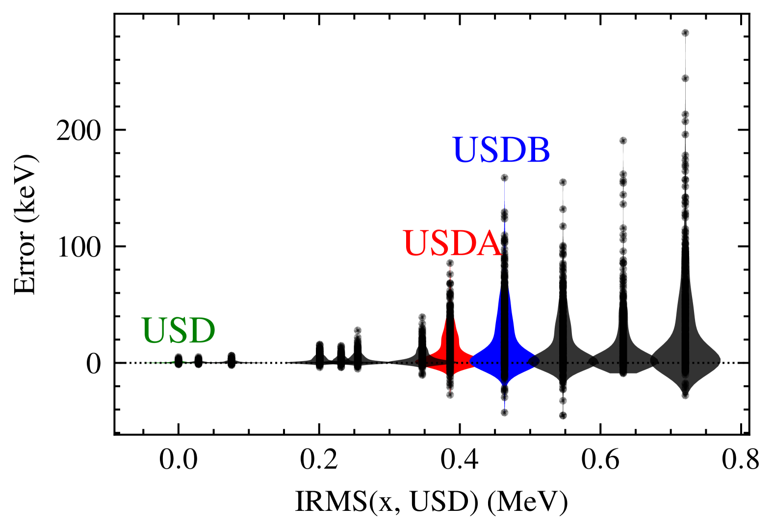
Table 2 summarizes the performance of the , model for each of the 12 validation tests shown in Fig. 1. We find the emulator error to be almost completely negligible until the test interaction exceeds 250 keV IRMS relative to USD, and acceptably small for all other tests. The error introduced by the emulator is therefore sufficiently small to ignore for the purposes of fitting new interactions without including any correction term.
| Test | IRMS(USD) | DRMS | 10-th | 50-th | 90-th |
|---|---|---|---|---|---|
| USD | 0 | 0.8 | -0.006 | 0.1 | 1 |
| Rnd. 1 | 28 | 0.8 | -0.005 | 0.1 | 1 |
| Rnd. 2 | 75 | 1 | -0.007 | 0.1 | 2 |
| Rnd. 3 | 200 | 4 | -0.005 | 0.4 | 7 |
| Rnd. 4 | 230 | 3 | -0.007 | 0.4 | 5 |
| Rnd. 5 | 250 | 5 | -0.006 | 0.6 | 8 |
| Rnd. 6 | 350 | 7 | -0.005 | 0.9 | 13 |
| USDA | 390 | 18 | -0.010 | 3.0 | 34 |
| USDB | 460 | 32 | -0.010 | 5.4 | 56 |
| Rnd. 7 | 550 | 28 | -0.040 | 3.2 | 50 |
| Rnd. 8 | 630 | 28 | -0.008 | 1.7 | 43 |
| Rnd. 9 | 720 | 48 | -0.005 | 4.9 | 82 |
In this section, we have shown that the EC model can be used to efficiently and effectively emulate the FCI SM without significant loss of accuracy. In particular, we expect that within the domain of input interactions we expect to encounter, the typical error introduced by the EC emulator on the predicted energy levels is on the order of keV, which is an order of magnitude smaller than the expected theoretical uncertainty of the untruncated shell model. If we find that the fitted interaction obtained with the EC model were much further away in IRMS from the training set than expected, we would need to retrain the model or perform other validation steps to ensure that the EC model retained its accuracy.
III Results
Eventually, the goal for any UQ approach is to credibly asses the expected error of any given model prediction. In the next few sections, we show that a direct extension of previous efforts to assess the uncertainty of the phenomenological SM, and in particular using the USDB interaction, results in a significant underestimation of the reported uncertainty. We first reproduce earlier methods using the the LC -minimization method (section III.1), then directly extend the method simply by replacing minimization with MCMC (section III.2). This extension ensures that we explore a wider range of the parameter space searching for alternative minima, and at the same time lifting the previous assumption that the distribution of model parameters can be described by a multivariate normal. As a result, we find a systematic underestimation of the uncertainty by a factor of 3. Finally, we suggest a first correction to these methods in order to obtain credible predictive intervals by increasing a hyperparameter of the fit () to obtain the desired empirical behavior: predictive intervals with widths that reflect the actual expected model error.
III.1 LC minimization
We first repeat the method used by Brown and Richter [15] to reproduce the USDB interaction, but using the EC emulator in place of the full SM. We used the EC emulator with a maximum of 40 samples with 10 levels per sample (, model). There are two reasons to repeat this method. First, we can further validate the effectiveness of using the EC emulator by reproducing the earlier results of Brown and Richter. Second, by re-computing the most important linear combinations of matrix elements, we can pre-optimize our MCMC fitting procedure to be discussed in Sec. III.2.
We conducted a number of tests to explore the convergence of this EC+LC method. First, we replicated the conditions used in Ref. [15], initializing the 66 nuclear matrix elements with the USD values and taking , with keV. Then we varied either 30 (USDA) or 56 (USDB) linear combinations with the largest error-matrix eigenvalues. Following the procedure of Ref. [15], the remaining 36 or 10 linear combinations were set to the renormalized G-matrix elements of Ref. [7] (RGSD). The data used in the fit were the same 77 ground states energies and 531 excitation energies of Ref. [15]. We follow the decision of Brown and Richter, fixing the ground state energies to be the uncorrected binding energies coming directly from the SM, and compare to the experimental ground state binding energies after “correction” by . (See equation (7).) Meanwhile, the excited states are fitted directly as excitation energies , where is the ground state energy of a given nucleus.
Convergence of the model residuals and matrix elements is reached in 5 iterations. The DRMS value falls to 133 keV, and the IRMS of the LC constrained matrix elements with respect to USDB is 12 keV. If the fitting conditions were identical, the difference should approach zero. As a reference, the IRMS between USDA and USDB is about 262 keV. We repeated these calculations using the exact SM and found that the converged DRMS for was also 12 keV, showing that the emulator introduces negligible error to the method (see Table 1). We believe this nonzero residual relative to the published USDA and USDB interactions to be caused by differences in numerical precision of the diagonalization algorithms used, in the storing of matrix elements, or also in the precision that the code operates overall. This explanation is further supported by the fact that when we compare our exact SM predictions to the data using the published USDB interaction, we find a DRMS of 131 keV, which is marginally larger than the reported 130 keV [15]. The EC emulator introduces a few keV in DRMS (about 3 keV), and on the order of tens of keV in IRMS. Compared to the typical expected error for a SM calculation in the -shell (100 keV), this discrepancy is negligible.
When we repeated the fit while varying 30 LCs (), the converged DRMS using the EC model was 175 keV, and the IRMS with respect to USDA was 10 keV. We also conducted 22 other replication studies using different initial conditions for the LC minimization algorithm. Holding the number of LCs fixed, we varied the initial matrix elements and found that the matrix elements converged to the same values to within numerical precision. The linear transformations given by the unitary matrix also converged to within numerical precision. We conclude that the results are insensitive to the initial matrix elements.
Next, we reproduced Figure 4 of Ref. [15] which shows, as a function of the number of linear combinations varied , the DRMS and the IRMS relative to RGSD, USDA, and USDB. As expected, the IRMS relative to USDA and USDB are minimized at LCs, respectively (see Fig. 2). The depth of these minima and the sharp change compared to using just one less linear combination, show that the IRMS deviation is highly sensitive to changes in the fitting procedure.
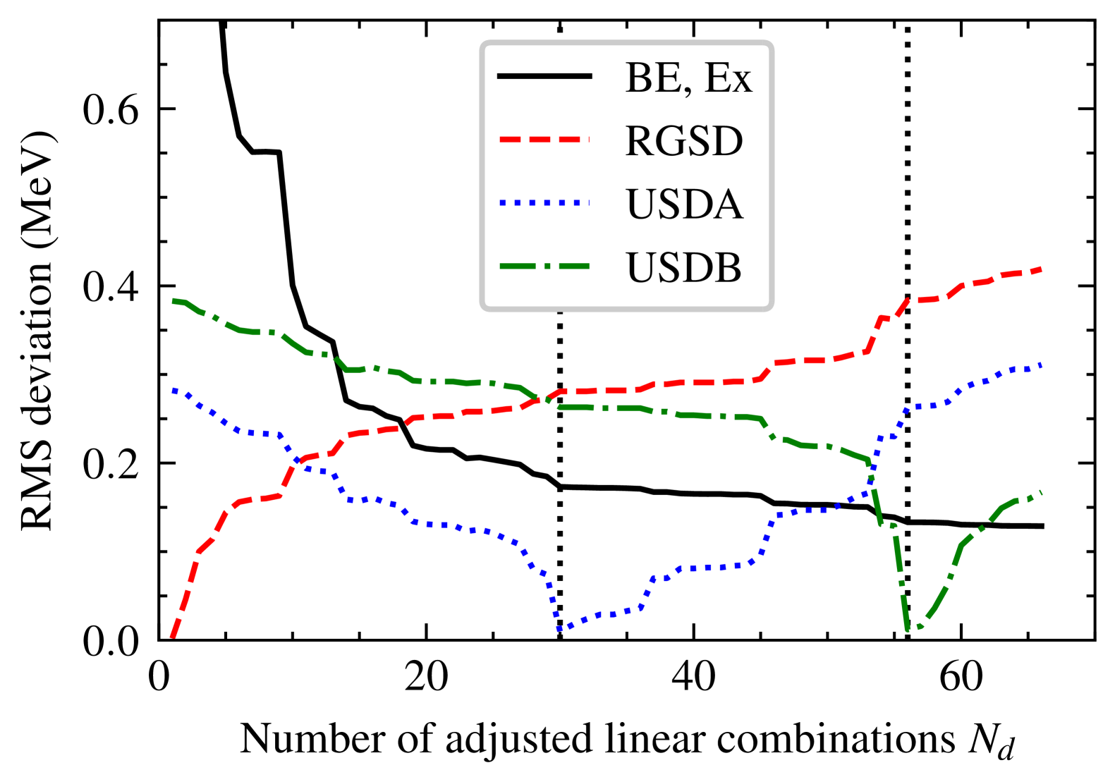
The high sensitivity of the IRMS, demonstrated in Fig. 2, is a direct result of the established finding [15, 20] that the constraints placed on the LCs are concentrated to just a few leading terms (the terms best constrained). We argue that rather than restricting the least constrained parameters to some constant prior value (here, and in Ref. [15], the RGSD value), it is more appropriate to maintain the value obtained from the fit and to report the estimated uncertainty.
In Fig. 3, we illustrate how the LC-transformed USDA and USDB interaction matrix elements compare to the optimal values from our fit with . We used the linear transformation which defines the optimal LCs with to transform the RGSD, USDA, and USDB matrix elements. The plot shows each set of LCs relative to the optimal values . Above and below , we shade in the region given by using the diagonal error matrix as defined in Sec. II.1.2. The minimization which produced the and uncertainties used keV as in Ref. [15]. This constant sets the absolute scale of the uncertainties of the resulting matrix elements, as the experimental uncertainties are generally much smaller. We also show the uncertainties obtained assuming a MeV uncertainty.
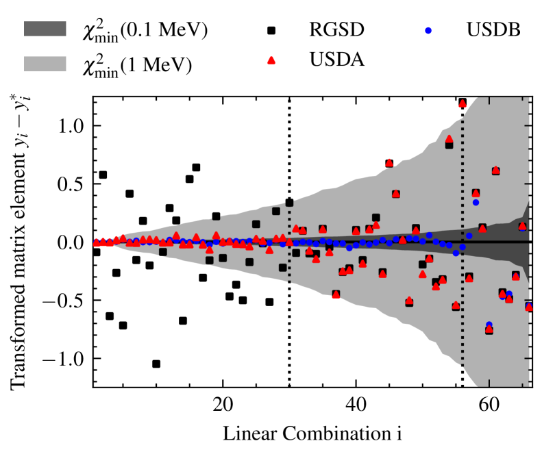
Fig. 3 confirms that below the LC, USDA is equal to the optimal values from the fit, while above LCs USDA is equal to RGSD (by construction, following Ref. [15]). The same is true for USDB below and above . In the context of the estimated uncertainties of the optimal fit, most transformed RGSD values are more than 1 standard deviation away (shown by the shaded region) from the optimal fit values .
We found that to envelop the RGSD predictions above 30 LCs, used in the fit has to be increased by a factor of 10 to 1 MeV. Given that the RGSD matrix elements are significantly inconsistent with the experimental constrains, one might posit that an improved SM interaction, without over-fitting, could be obtained by retaining all 66 linear combinations from the fit. We investigate this hypothesis in the next section.
To conclude this section on the LC -minimization study, we found that EC can serve as an efficient and sufficiently accurate emulator of the full SM for the purposes of fitting interaction matrix elements. We were able to to reproduce the USDA and USDB matrix elements using the EC emulator, which sped up the fitting procedure by a factor of 800. These findings will be leveraged in the future to construct novel interactions in regions where SM calculations are significantly more costly to compute and thus a global fit has not been attempted.
III.2 LC Markov chain Monte Carlo
In this section, we first present three new interactions dubbed USDBUQ, USD66, and USDBUQ-500. All three are produced with the same experimental data corpus as USDA/B, and using the same set of linear combinations found in Section III.1 with for USDBUQ and for USD66. USDBUQ is a reproduction of USDB, except with parametric UQ using MCMC. We note that some measure of parametric uncertainty is readily obtained from the the LC -minimization method via the final covariance matrix obtained by the fitting procedure. This covariance matrix represents the normal distribution approximation to the true covariance; in principle higher moments are needed to describe the distribution but most fitting protocols go up to the second. Whether this approximation is good or not can be rigorously tested via MCMC.
USD66 is a generalization of USDBUQ wherein all 66 linear combinations are varied or, alternatively, all matrix elements are considered as free parameters. It has already been shown in previous work [15] that increasing the number of LCs does not meaningfully increase the overall accuracy of the model. Our results support this finding, but an important question we wish to answer with USD66 is: does the increased uncertainty of the 66 matrix elements result in an increased uncertainty of observables other than the spectra? To answer this question, we performed two sets of calculations for specific E2 transitions in 24Mg.
For USDBUQ (), we used a fixed keV. For USD66 (, varying all linear combinations), we treated as an unknown parameter which was simultaneously varied along with the matrix elements, similar to the procedure followed in [31]. The prior distribution for was chosen to be a truncated normal with a mean of 130 keV and standard deviation of 10 keV (min/max bounds were set to 0 and 200 keV, respectively).
We then show that both USDBUQ and US66 underestimate the parametric uncertainty, and yield predictive intervals which greatly underestimate the true model error (or, deviation from experiment). This underestimation is related to the idea of overfitting, yet requires a different remedy. The linear combination methods of Refs [15], or its extension using divided training and test data [32], address overfitting by reducing the number of degrees of freedom of the model. Our solution for underestimated uncertainties is instead to increase the range of parameters we consider credible while keeping the number of parameters fixed. In Section III.2.3, we show that we can approximately recover credible confidence intervals in our uncertainty quantification, not by decreasing the degrees of freedom, but by increasing the scale of . This procedure results in our third interaction, USDBUQ-500. The interaction samples for all three interactions are provided as supplemental material.
III.2.1 USDBUQ
In this section, we discuss a refit of the USDB interaction using MCMC. We call this new interaction USDB with uncertainty quantification (USDBUQ). We keep all other aspects of the fit the same, except that we increase the theoretical uncertainty from 100 keV to 130 keV to reflect the empirical DRMS achieved by the USDB interaction. We used the same set LCs obtained in Section III.1 in order to directly compare the MCMC method to chi-squared minimization. We again varied the leading linear combinations of the 66 matrix elements, while the remaining 10 were held fixed at the RGSD values. The prior distribution is taken to be a multivariate normal with means equal to the optimal values from the the LC -minimization method fit, but with standard deviations equal to 10 the uncertainty values from the the LC -minimization method fit, as obtained from the diagonal of the resulting covariance matrix. This wide prior allows the algorithm to search for alternative solutions while keeping the parameter space within the domain of validity of the EC model.
We generated 10000 iterations using 560 walkers (5.6 million samples total) using the emcee [33] affine-invariance ensemble sampler. (Across the 77 nuclei, this means more than 430 million SM calculations performed with the EC emulator.) Posterior distribution statistics were computed using the last sample of each Markov Chain.
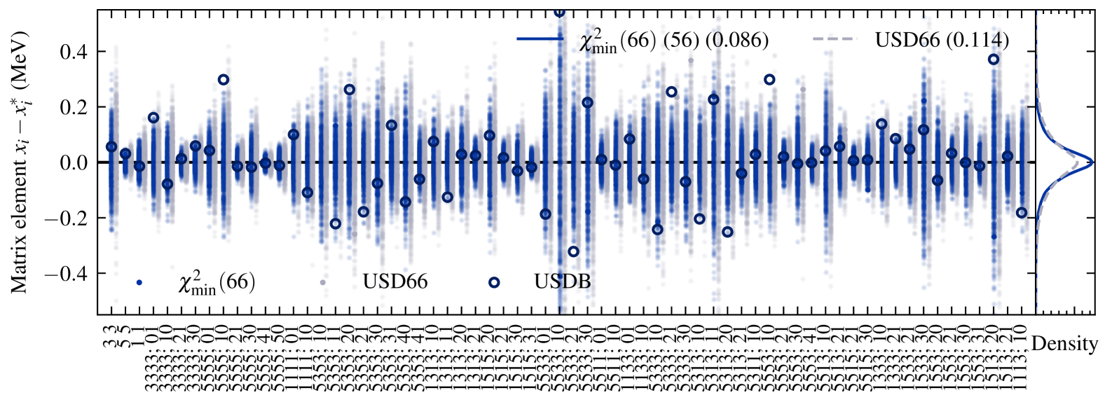
Figure 4 shows the marginal distribution of each of the 3 single particle energies and 63 TBMEs, plotted relative to the optimal set of matrix elements found with the LC -minimization method. The small subpanel shows the overall variance of the matrix elements obtained with the two methods, and for the single value of USDB. For comparison, we draw 560 samples from the multivariate normal posterior of the LC fit; the means are equal to the optimal LCs , and the variances equal to the diagonal error matrix . We emphasize that in the LC basis the multivariate normal contains no non-diagonal terms.
Then, for each sample, the LCs are transformed to interaction matrix elements with the transform : . Similarly, the yellow (placed on the right) clusters of points correspond to samples from the new USDBUQ interaction, which are transformed from the LCs by the same transform .
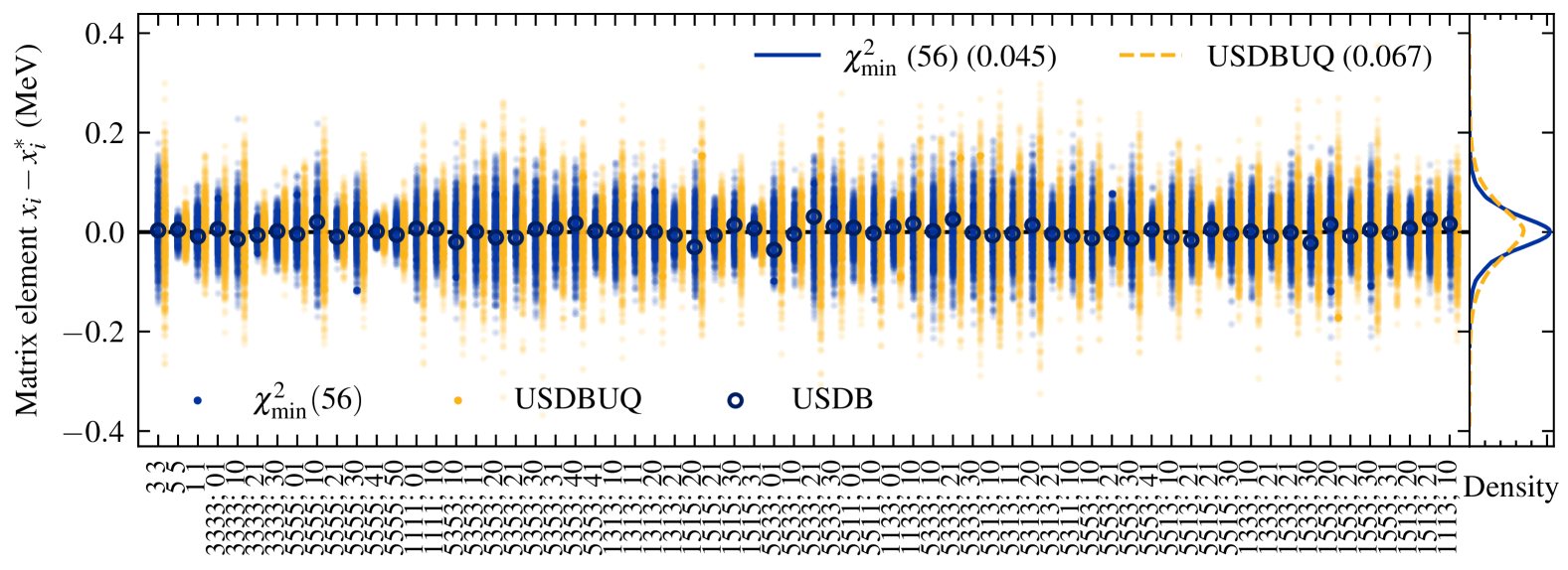
Using the distribution of matrix elements shown in Fig. 4, we find that the MCMC approach yields mean values compatible with the LC fit: the standard deviation of the matrix elements around for the LC -minimization method and USDBUQ are about 45 keV and 67 keV, respectively (i.e. the half-widths of the distributions shown in the subpanel of Fig. 4). USDBUQ’s increased uncertainty in the matrix elements is a direct result of using an increased keV, compared to the 100 keV value used for the the LC -minimization method. What else is clear from Figure 4 is that some matrix elements, such as the , single particle energies, are much more constrained by the data than others. Some of the least constrained matrix elements include the SPE.
In summary, USDBUQ has the same mean matrix elements determined with LC -minimization, but with uncertainties larger by about 50%, owing to the larger keV used in the fit. 560 independent walkers searched the parameter space within ten standard deviations of the the LC -minimization method minimum, and no other minimum was found. The posterior distribution of linear combinations also remained uncorrelated, suggesting that the linear transform identified with the -minimization is robust.
III.2.2 USD66
Driven by the results shown in Fig. 3, we analyze a new interaction defined by fitting all 66 linear combinations to the data. While this approach allows us to obtain marginally better agreement with the data, that is not our goal. More importantly, varying all 66 parameters avoids arbitrarily fixing the least-constrained linear combinations of the final 66 interaction matrix elements (to the RGSD ones). This increase in accounted-for uncertainty will allow us to test whether these additional degrees of freedom will increase the variance of other observables not included in the fit.
As with USDBUQ, we use the results of the LC -minimization method both to define the set of linear combinations that are used as an independent set of “orthogonal” model parameters, but also to obtain a prior for those 66 parameters. Since we are now interested not only in the optimal set of matrix elements, but their uncertainty and covariance as well, we revisit our assumptions about the exact size of ; assuming a larger will directly result in a larger uncertainty obtained from the fit, as demonstrated in the case of USDBUQ (Fig. 4, right panel).
As an extra step, we now further treat the hyperparameter as a random variable as was done in Ref. [31], and allow the MCMC algorithm to optimize its value. Note that the log-likelihood function defined in Eq. (9) has a term proportional to the determinant of the covariance matrix (essentially, ), which naturally protects against an ever-growing .
We produced approximately 10000 MCMC iterations with 670 walkers, resulting in 6.7 million samples. Again, the posterior distribution statistics were computed using the last sample of the Markov Chain (Fig. 5). Just as in the case of USDBUQ, the uncertainties using the MCMC method are marginally larger than those of the LC -minimization method. We also found that the posterior distribution for keV, rather close to the 130 keV value selected for the USDBUQ fit. Recall that the the LC -minimization method method assumed =100 keV.
What is most notable about these USD66 results, however, is that the total variance in some matrix elements is much larger than for USDBUQ. The overall mean uncertainty of the matrix elements for the LC -minimization method and MCMC are about 86 keV and 114 keV, respectively (i.e. the half-widths of the distributions shown in the subpanel of Fig. 5).
Overall, the mean uncertainty for the matrix elements of USD66 (114 keV) is about 70% larger than for USDBUQ (67 keV). This increase in reported uncertainty is expected since we allow additional degrees of freedom to vary within the limits set by the data; for USDBUQ, 10 of the 66 linear combinations were held fixed. It remains to be answered whether or not this increase in matrix element uncertainty has consequences for other observables. Nonetheless, we argue that the full range of parameters compatible with the data should be reported as part of a complete uncertainty analysis.
III.2.3 Uncertainty estimation and USDBUQ-500
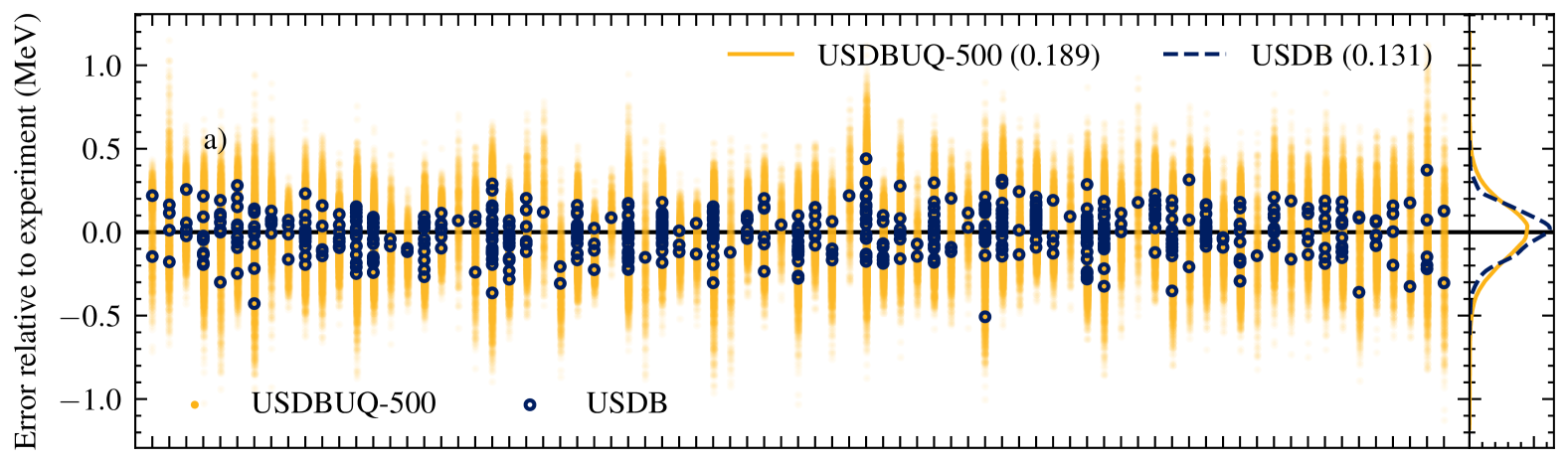
In this section we turn our focus to the more fundamental question of what is the actual uncertainty of a SM prediction. One could expect that barring any model deficiency, the deviation of theoretical predictions from experiment would follow a normal distribution of a width similar to the DRMS of the interaction, augmented by (added in quadrature). However, as shown in Fig. 6 (bottom panel) this is not the case. We demonstrate the the assignment of an uncorrelated 130 keV uncertainty per energy level leads to an underestimation of the uncertainty of predictions.
Specifically, Fig. 6 shows the performance of the new interactions for predicting the 608 energies across the 77 nuclei in the training set. The horizontal axis of the main panel groups subsets of energies by nucleus. The vertical axis of either plot shows the residual/error between the SM predictions and either (a) the experimental value, or (b) the mean model prediction. For reference, we show the errors for the USDB interaction in dark blue open-circles, with one marker per energy level. For example, 39K has two energy levels in the training set, so there are two open circles for USDB. The main results shown are 560 random samples from the new USDBUQ interaction, resulting in (the yellow, left set of) clusters for the energy levels of each nucleus. For USD66, shown in gray clusters, there are 670 samples. The shaded green in Fig. 6a indicates the keV used to fit the USDBUQ matrix elements (close to the fitted value of keV for USD66.)
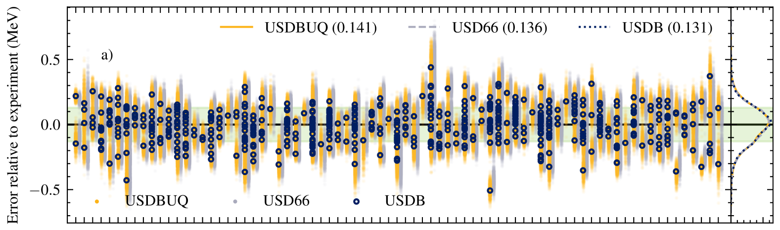
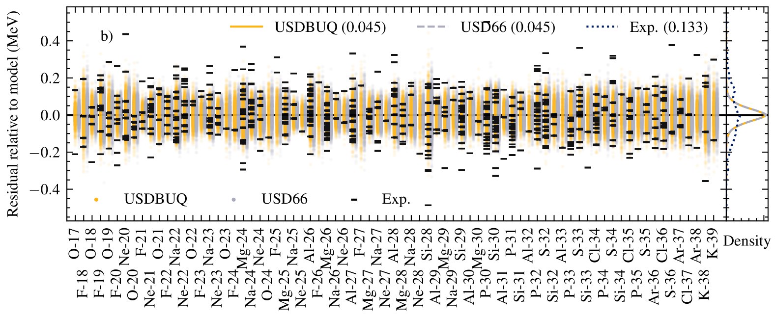
The small subpanels of Fig. 6a and 6b show the overall distribution of errors and residuals from the main panels. Despite the fact that the USDBUQ interaction has a range of predictions for each energy level, the overall distribution of errors is comparable to USDB. The DRMS obtained with the USDB interaction is 131 keV, while for USDBUQ across all 560 samples it is 141 keV. This slight DRMS increase is due to the spread in predictions; if we use the mean value of the USDBUQ matrix elements, the DRMS is 133 keV. The USD66 interaction also shows a similar overall DRMS. For some nuclei, it is clear that the increased number of degrees of freedom decreases the error, such as for 39K, 38Ar, and 17O, where the distributions of residuals move towards zero. However, there are also levels where the errors increase. The sum effect across all 608 energies is to decrease the DRMS from the USDBUQ value of 141 keV to 136 keV for USD66.
Fig. 6a shows that the distribution of residuals is indeed consistent with the assumed theoretical uncertainty of about 130 keV. However, the uncertainty for any given energy level, as estimated by the posterior distribution of matrix elements, is significantly smaller than the overall theoretical uncertainty: the standard deviation of the model predictions are, on average, about 45 keV per level for both USDBUQ and USD66.
Fig. 6b shows the same calculations as in 6a, except the origin has been shifted to the mean model prediction for each energy level instead of the experimental value. The inset panel showing the overall distribution solidifies the situation: the uncertainty estimate generated by fitting the interaction matrix elements underestimates the actual typical error of the SM. This result is not altered when increasing the number of parameters from 56 to 66 in moving from USDBUQ to USD66; while the average standard deviation of the matrix elements increases from 67 keV to 85 keV due to the increased degrees of freedom, the standard deviation of the predicted energy levels does not change (45 keV). Meanwhile, the DRMS (i.e. the empirical systematic error) decreases only marginally from 141 keV to 136 keV, and remains approximately 3 times larger than the parametric uncertainty.
In a typical application of parameter estimation with noisy measurements, one assumes that the model is “perfect” and thus interprets the uncertainty that arises from fitting the model parameters to the data (parametric uncertainty) as the total prediction uncertainty. However, as the number of data points () grows, one expects the uncertainty of the quantity of interest to fall at a rate of . Thus, for a very large number of points, one would have nearly zero uncertainty in the prediction.
While this is a desirable situation in the absence of model defects, that is not the situation for nuclear physics models like the SM. Indeed, we know that approximations and omissions exist in the SM and thus there is no parameter set that can coherently describe all experimental data. At the same time, the data itself has little to essentially no uncertainty. Thus, as mentioned above, if we include more and more data in the SM fit, we will be “more confidently wrong” in our predictions, i.e. we will have tighter error bars in predictions that are not in agreement with experiment. Such an outcome would be contradictory to what one would ideally expect from a UQ approach under these conditions, namely, that the prediction error would remain relatively constant after a certain number of data points is included in the fit.
To formalize this discussion in terms of the likelihood function, one might multiply the uncertainties by the reciprocal factor, , or (equivalently) multiply the covariance matrix by . We found that this approach greatly overestimates the uncertainty, which is unsurprising since the assumption of independent degrees of freedom is simply the opposite extreme (see discussion here [34]). In reality, the residuals are correlated.
As an alternative approach, we have chosen to empirically test the coverage and increase the assumed uncorrelated uncertainty until a satisfactory agreement is achieved; that is, until the distribution of model uncertainty coincides with the distribution of model errors (Fig. 7). As increases, the percentage of experimental data covered by the central -percent credible interval predicted by the model fit approaches the 45∘ line.
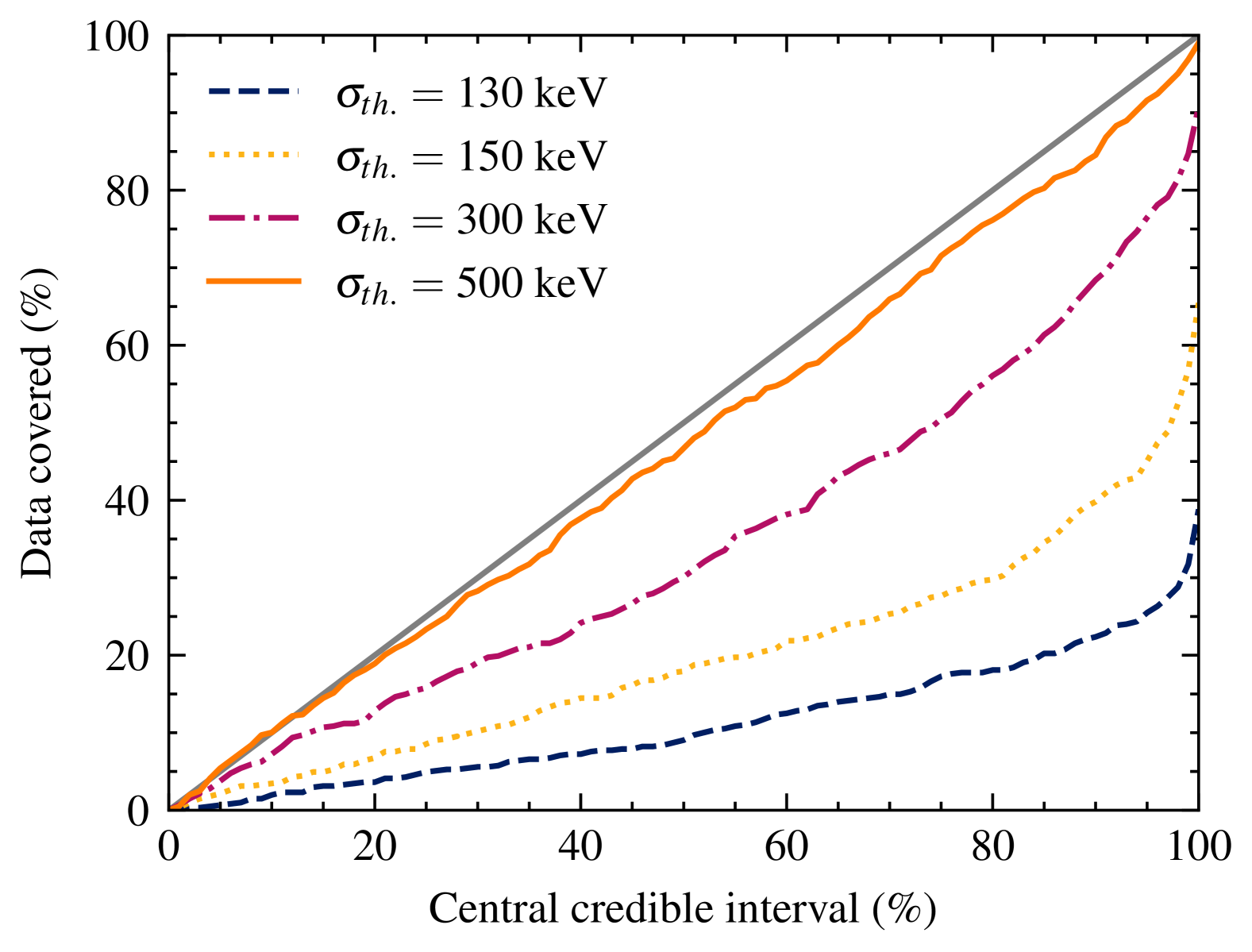
As a reminder, the value used to produce USDBUQ and USD66 was keV because this value provides statistical agreement with the data assuming independent normal errors. We find that to obtain a reasonable coverage of the data, we instead must increase the assumed uncorrelated uncertainty to keV. As will be discussed, however, this does not suggest an expected theoretical uncertainty of 500 keV across all predictions.
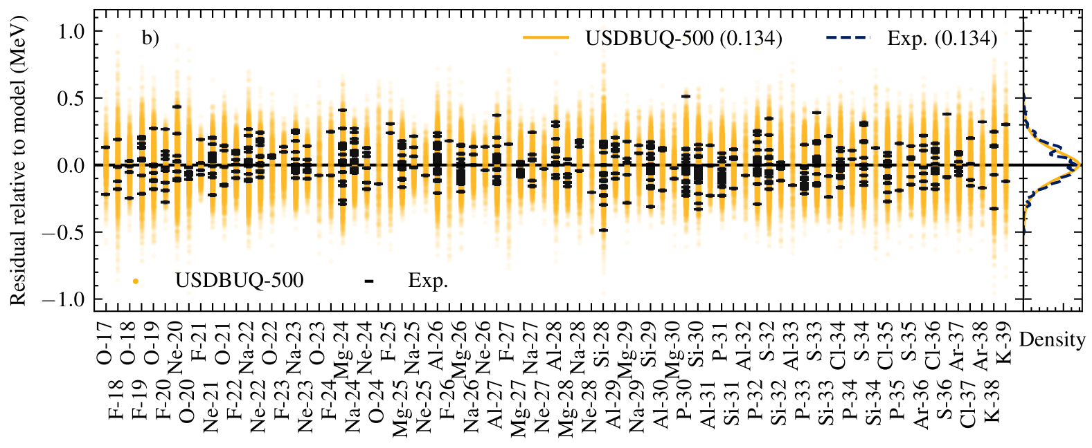
Figure 8 shows the performance of the final interaction presented in this paper, USDBUQ-500, which was fit identically to USDBUQ but with keV. In this case, the standard deviations for both the model predictions and the residuals of experimental values relative to the mean model prediction are both 134 keV. The overall distribution of residuals in both cases is roughly normal with mean zero. However, due to the same correlations that cause keV underestimating the true model uncertainty, keV does not result in a mean error as large as 500 keV. Instead, using keV, the DRMS of the entire distribution of prediction across the energies increases to only 189 keV (up from 135 keV using keV). The error of the mean model prediction using this increased theoretical uncertainty remains approximately unchanged, increasing from 133 keV to 134 keV. In summary, a single random interaction drawn from the USDBUQ-500 interaction has an expected DRMS of 190 keV; a large number of samples drawn from USDBUQ-500 will produce a spread in predictions with an average width of about 134 keV per level (averaged across energy levels for many nuclei), and the experimental value likewise will be on average 134 keV away from the mean prediction. We suggest that USDBUQ-500 provides a more credible uncertainty analysis than previous attempts.
III.2.4 Monopole energies and quadrupole transitions
Next, we compare specific features of the interactions, the single-particle energies and monopole energies. Furthermore, we wish to test whether the increased parametric uncertainty described in the USD66 interaction results in greater uncertainty in transition quantities.
The single-particle energies , with , are a key part of the interaction as they represent the dominant mean-field interaction among all the nucleons. The monopole energies are sums of those two-body matrix elements which can be recast as a number operator, and therefore contribute to the effective single-particle energies. They are defined as:
| (18) |
The effective single-particle energies (ESPEs) are then given by , and we report the mean and standard deviations from each fit (along with USDB) in Table 3 .
| SPE/ESPE | USDB | USDBUQ | USD66 | USDBUQ500 |
|---|---|---|---|---|
| 2.112 | ||||
| -3.926 | ||||
| -3.208 | ||||
| -3.289 | ||||
| -6.897 | ||||
| -6.851 |
An important lesson obtained by comparing USDBUQ and USD66 single-particle energies is that while the increase in degrees of freedom in USD66 does not significantly increase the uncertainty (width) of the predicted single-particle energies, it does shift the minimum of the single-particle energy. On the other hand, if we appropriately increase the uncertainty to account for the SM defect (resulting in the USDBUQ-500 interaction), the difference between the two minima is no longer significant at the 1 level. For USDBUQ500 the size uncertainties are now roughly two-to-three times larger, which follows the increase in uncertainty of the energy levels.
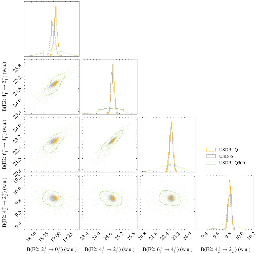
Finally, we compare the distribution of predictions for electric quadrupole transitions between low-lying states in 24Mg, using standard effective charges , [35]. We chose three transitions from the ground-state rotational band: , , , and one transition from the next rotational band built on the second state: . Fig. 9 shows the values for these four transitions in 24Mg. The experimental values for these transitions are shown along with the theoretical predictions in Table 4.
Both USDBUQ and USD66 interactions predict nearly identical means and uncertainties for the transition strengths, with the exception of the ground state transition which shows a slight splitting in the two interactions. The increased degrees of freedom and range of interaction matrix elements allowed by the USD66 interaction does not significantly increase the uncertainty in the predicted transition matrix elements. The USDBUQ-500 interaction with enhanced uncertainty predicts approximately the same mean transition strengths, with uncertainties increased by a factor of approximately 4-6. This increase brings the predicted theoretical uncertainty in transition strengths to roughly which, however, is still not in agreement with experiment; all four transitions are in fact inconsistent with their experimental values. The SM predictions are systematically smaller by roughly 50%, indicating that effective charges used under-estimate the collectivity contributed by particles outside of the valence space. This conclusion is supported by the observation from Fig. 9 that the transitions within the same rotational band are strongly positively correlated; if one transition value were corrected to its experimental value, these correlations would also bring the other two transitions in the band closer to the observed values.
| Exp (w.u.) | USDBUQ | USD66 | USDBUQ-500 | |
|---|---|---|---|---|
IV Conclusions
In this paper we have shown that EC can be used to emulate the SM with sufficient accuracy to fit SM interactions with negligible error. The speedup compared to the full SM scales as the cube of the dimension for the largest fitted system; for the sd-shell the speedup is roughly three orders of magnitude. This speedup is sufficient to use MCMC as the fitting algorithm, which we used to verify that the existing USDB interaction with 56 degrees of freedom is a global, although shallow, minimum. We note that once the emulator is constructed the runtime should be independent of model space, and thus the EC framework can be used for future, more computationally demanding, studies.
Since our interaction distribution obtained with MCMC is well approximated by the distribution found with the the LC -minimization method, we can conclude that there are no significant nonlinearities between the matrix elements and the energy spectra, which could have resulted in non-normal distributions in the interaction matrix elements. Again, this appears to be a global feature of SM interactions, confirming that the the LC -minimization method approach is indeed appropriate for future studies.
When it comes to uncertainty analysis, restricting the fitting procedure to fewer linear combinations (e.g. for USDB) underestimates the total parametric uncertainty of the matrix elements. However, this approach appears to have minimal impact on the uncertainty of either the energy levels or the transition probabilities. More importantly, we found that the assumption of uncorrelated uncertainties inherent to previous methods results in a factor of 3 underestimation of the matrix elements obtained from the fit. Any confidence interval obtained by sampling the parameter uncertainty with this underestimate will therefore systematically underestimate the true model error.
When the model defect is much larger than the experimental uncertainty, the model’s covariance contributes significantly to correlations in the residuals, which are modeled as independent with a diagonal covariance matrix. Our approximation of the covariance matrix as diagonal results in an un-modeled reduction in the uncertainty passed to the model parameters. We found by trial and error that we can remedy this underestimation by increasing the diagonal of the assumed covariance matrix until the average predicted model uncertainty matches the average model error. Using this approach, we report our new uncertainty quantified USDBUQ-500 interaction. When sampling from this distribution of matrix elements, predicted energy levels will have an expected mean error relative to experiment of 0 keV with a standard deviation of 190 keV (Fig. 8a). Meanwhile, the confidence intervals produced by sampling will approximate the probability for the experimental value to fall within that interval (Fig. 7). The average prediction for an energy level is expected to have a standard error of 134 keV, and the expected standard deviation of predictions for the same level are expected to match at 134 keV (Fig. 8b). Ideally, one should estimate the off-diagonal contributions to the covariance matrix and include them in the fit.
Acknowledgements.
Prepared by LLNL under Contract DE-AC52-07NA27344 with support from LDRD Project No. 23-ERD-023. We are grateful for insightful conversations with Cole Pruitt and Simone Perrotta regarding uncertainty quantification and model defects.References
- Mayer [1949] M. G. Mayer, Phys. Rev. 75, 1969 (1949).
- Haxel et al. [1949] O. Haxel, J. H. D. Jensen, and H. E. Suess, Phys. Rev. 75, 1766 (1949).
- Caurier et al. [2005] E. Caurier, G. Martínez-Pinedo, F. Nowacki, A. Poves, and A. P. Zuker, Rev. Mod. Phys. 77, 427 (2005).
- Nowacki et al. [2021] F. Nowacki, A. Obertelli, and A. Poves, Progress in Particle and Nuclear Physics 120, 103866 (2021).
- Otsuka et al. [2001] T. Otsuka, M. Honma, T. Mizusaki, N. Shimizu, and Y. Utsuno, Progress in Particle and Nuclear Physics 47, 319–400 (2001).
- Dao and Nowacki [2022] D. D. Dao and F. Nowacki, Phys. Rev. C 105, 054314 (2022).
- Hjorth-Jensen et al. [1995] M. Hjorth-Jensen, T. T. Kuo, and E. Osnes, Physics Reports 261, 125 (1995).
- Stroberg et al. [2019] S. R. Stroberg, H. Hergert, S. K. Bogner, and J. D. Holt, Annual Review of Nuclear and Particle Science 69, 307–362 (2019).
- Miyagi et al. [2020] T. Miyagi, S. R. Stroberg, J. D. Holt, and N. Shimizu, Phys. Rev. C 102, 034320 (2020).
- Coraggio and Itaco [2020] L. Coraggio and N. Itaco, Frontiers in Physics 8, 10.3389/fphy.2020.00345 (2020).
- Dikmen et al. [2015] E. Dikmen, A. F. Lisetskiy, B. R. Barrett, P. Maris, A. M. Shirokov, and J. P. Vary, Phys. Rev. C 91, 064301 (2015).
- Sun et al. [2018] Z. H. Sun, T. D. Morris, G. Hagen, G. R. Jansen, and T. Papenbrock, Phys. Rev. C 98, 054320 (2018).
- Brown and Wildenthal [1988] B. A. Brown and B. H. Wildenthal, Annual Review of Nuclear and Particle Science 38, 29–66 (1988).
- Honma et al. [2002] M. Honma, T. Otsuka, B. A. Brown, and T. Mizusaki, Physical Review C 65, 061301 (2002).
- Brown and Richter [2006] B. A. Brown and W. A. Richter, Phys. Rev. C 74, 034315 (2006).
- Utsuno et al. [2012] Y. Utsuno, T. Otsuka, B. A. Brown, M. Honma, T. Mizusaki, and N. Shimizu, Progress of Theoretical Physics Supplement 196, 304 (2012).
- Caurier et al. [2014] E. Caurier, F. Nowacki, and A. Poves, Phys. Rev. C 90, 014302 (2014).
- Lubna et al. [2020] R. S. Lubna, K. Kravvaris, S. L. Tabor, V. Tripathi, E. Rubino, and A. Volya, Phys. Rev. Res. 2, 043342 (2020).
- Magilligan and Brown [2020] A. Magilligan and B. A. Brown, Phys. Rev. C 101, 064312 (2020).
- Fox et al. [2020] J. M. R. Fox, C. W. Johnson, and R. N. Perez, Physical Review C 101, 10.1103/physrevc.101.054308 (2020).
- Fox et al. [2023] J. M. R. Fox, C. W. Johnson, and R. N. Perez, Phys. Rev. C 108, 054310 (2023).
- Yoshida et al. [2018] S. Yoshida, N. Shimizu, T. Togashi, and T. Otsuka, Phys. Rev. C 98, 061301 (2018).
- Wildenthal [1984] B. Wildenthal, Progress in Particle and Nuclear Physics 11, 5–51 (1984).
- Chung [1976] W. Chung, Empirical renormalization of shell-model Hamiltonians and magnetic dipole moments of sd-shell nuclei, Ph.D. thesis, Michigan State University (1976).
- Gelman et al. [1995] A. Gelman, J. B. Carlin, H. S. Stern, and D. B. Rubin, Bayesian data analysis (Chapman and Hall/CRC, 1995).
- Frame et al. [2018] D. Frame, R. He, I. Ipsen, D. Lee, D. Lee, and E. Rrapaj, Phys. Rev. Lett. 121, 032501 (2018).
- König et al. [2020] S. König, A. Ekström, K. Hebeler, D. Lee, and A. Schwenk, Physics Letters B 810, 135814 (2020).
- Yoshida and Shimizu [2022] S. Yoshida and N. Shimizu, Progress of Theoretical and Experimental Physics 10.1093/ptep/ptac057 (2022).
- Sarkar [2022] A. Sarkar, Eigenvector Continuation: Convergence and Emulators, Ph.D. thesis, Michigan State University (2022).
- Volya [2024] A. Volya, alvolya/cosmo: Cosmo v5.0.0 - initial release (2024).
- Pruitt et al. [2023] C. D. Pruitt, J. E. Escher, and R. Rahman, Phys. Rev. C 107, 014602 (2023).
- Purcell et al. [2024] J. A. Purcell, B. A. Brown, B. C. He, S. R. Stroberg, and W. B. Walters, Improving the predictive power of empirical shell-model hamiltonians (2024), arXiv:2412.09917 [nucl-th] .
- Foreman-Mackey et al. [2013] D. Foreman-Mackey, D. W. Hogg, D. Lang, and J. Goodman, Publications of the Astronomical Society of the Pacific 125, 306–312 (2013).
- Pruitt et al. [2024] C. D. Pruitt, A. E. Lovell, C. Hebborn, and F. M. Nunes, The role of the likelihood for elastic scattering uncertainty quantification (2024), arXiv:2403.00753 [nucl-th] .
- Richter et al. [2008] W. A. Richter, S. Mkhize, and B. A. Brown, Physical Review C 78, 10.1103/physrevc.78.064302 (2008).