Investigating the Temperature Sensitivity of UV Line Ratios in the 280 nm Region of Solar-like Stars

Abstract

Stellar UV spectra are fundamental diagnostics of physical and magnetic properties of stars. For instance, lines like Mg II at 280 nm serve as valuable indicators of stellar activity, providing insights into the activity levels of Sun-like stars and their potential influence on the atmospheres of orbiting planets. On the other hand, the effective temperature ($T_{eff}$) is a fundamental stellar parameter, critical for determining stellar properties such as mass, age, composition and evolutionary status. In this study, we investigate the temperature sensitivity of three lines in the mid-ultraviolet range (i.e., Mg II 280.00 nm, Mg I 285.20 nm, and Si I 286.15 nm). Using spectra from the International Ultraviolet Explorer (IUE), we analyze the behavior of the ratios of their corresponding indices (core/continuum) for a sample of calibrating solar-like stars, and find that the ration R = Mg II/Mg I best traces $T_{eff}$ through a log-log relation. The $T_{eff}$ estimated using this relation on a test-sample of solar-like stars agree with the $T_{eff}$ from the literature at the 95% confidence level. The observed results are interpreted making use of Response Functions as diagnostics. This study extends the well-established use of line depth ratio-temperature relationships, traditionally applied in the visible and near-infrared ranges, to the mid-UV spectrum. With the growing interest in stellar UV spectroscopy, results presented in this paper are potentially relevant for future missions as HWO, MANTIS and UVEX.

1 Introduction

The UV stellar spectral region and individual lines hold great significance in both stellar and planetary physics. UV studies have revolutionized our understanding of massive stars and their stellar winds (e.g., Hillier, 2020), while UV lines serve as valuable tools for refining physical models of stellar upper atmospheres (e.g., Loyd et al., 2021). Furthermore, the UV region of stellar spectra is crucial for understanding star-exoplanet interactions. Actually, variations in stellar UV irradiance, linked to magnetic activity, significantly impact exoplanet atmospheres, driving short-term changes in the middle atmosphere and long-term climate shifts, as well as altering their chemical composition via photodissociation and inducing atmospheric erosion processes (see, e.g., Sanz-Forcada et al., 2010; Tilley et al., 2019; Reda et al., 2023). For oxygen-rich planetary atmospheres, as in the case of Earth, the 200-300 nm spectral region is particularly important, as it governs the formation and destruction of ozone, a key component of the stratosphere (e.g., Bordi et al., 2015; Lovric et al., 2017). Therefore, characterizing the properties of UV lines in relation to stellar parameters, especially for Sun-like stars considered potential hosts for habitable planets, is of fundamental importance. The effective temperature ($T_{\rm eff}$) is one of the most important stellar parameters and serves as a pivotal parameter in the study of stellar atmospheres, playing a crucial role in inferring properties such as mass, age, surface gravity, and evolutionary status, along with providing insights into the star’s chemical composition. Various techniques exist to determine $T_{\rm eff}$, with the primary method relying on direct calculation of the radius of a star and absolute luminosity. However, this approach is limited to nearby stars. Alternative methods based on color-temperature relations (e.g., Alonso et al., 1996; Casagrande et al., 2021) or high-resolution spectroscopy (see e.g., Gehren, 1981; Cayrel & Cayrel, 1963; Lind et al., 2012) become essential for the more distant ones. Spectroscopic techniques, especially those that focus on stellar absorption lines, provide a more robust avenue for the determination of $T_{\rm eff}$, as they are largely unaffected by interstellar extinction. One notable method is the use of line depth ratios (LDRs), which entails measuring the relative strengths of absorption lines with different excitation potentials. This technique, first introduced by Gray & Johanson (1991), uses the temperature-dependent behavior of these lines to achieve precise temperature estimates. Recent studies have expanded this method across a range of stellar classifications and spectral features, demonstrating its versatility and effectiveness in diverse contexts, including the analysis of variable stars (see Caccin et al. 2002; Kovtyukh et al. 2006, 2023; Biazzo et al. 2007; Fukue et al. 2015; Afşar et al. 2023; Taniguchi et al. 2018, 2021; Jian et al. 2019; Matsunaga et al. 2021, and references therein). The estimate of the effective temperature in radial variables (Cepheids, RR Lyrae) is, indeed, a challenging problem, since typical radial variables experience variations of the order of one thousand degrees along the pulsation cycle, while the surface gravity changes by 0.2/0.3 dex and the micro-turbulent velocity can change from two to four km/s (Bono et al., 2024). This means that accurate estimates of the atmospheric parameters from high-resolution spectra and, in particular, of the effective temperature are required to provide accurate elemental abundances.

In this paper, we evaluate the temperature sensitivity of three line ratios in the middle ultraviolet range (MUV, 200–300 nm). For this purpose, we used spectra from the International Ultraviolet Explorer (IUE) space telescope, pioneering mission that provided a homogeneous and extensive database of stellar UV spectra. IUE operated continuously for 18 years, from 1978 to 1996, with two spectrographs: the long-wavelength spectrograph in the wavelength range of 185.0 to 330.0 nm (MUV, i.e., middle-UV) and the short-wavelength spectrograph in the range of 115.0 to 200.0 nm (FUV, i.e., far-UV). With the growing interest in stellar UV spectroscopy, several new missions are operational or planned to be launched in the near future, such as CUTE (Egan et al., 2018), HWO (National Academies of Sciences, Engineering & Medicine, 2021), MANTIS (Indahl et al., 2024), MAUVE (Majidi et al., 2024) and UVEX (Kulkarni et al., 2021), including near-UV (NUV) observations.

Although most of the radiative energy in the Sun is distributed mainly in visible areas, it is well known that the UV component contributes the most to the variability of the bolometric flux induced by magnetic activity (Yeo et al., 2015; Berrilli et al., 2020; Ermolli et al., 2003, 2013). The MUV spectral region (180-300 nm), in particular, contains a wide variety of spectral features that may serve as diagnostics for key stellar parameters, such as effective temperature, surface gravity, and metal abundance (Fanelli et al., 1990). In addition, this wavelength range has been extensively studied due to the presence of lines considered excellent proxies for magnetic chromospheric activity in the Sun and in F-G-K stars, such as Mg II at 280.0 nm and Mg I at 285.2 nm (Schrijver et al., 1992; DeLand & Marchenko, 2013; Heath & Schlesinger, 1986; Viereck et al., 2004; Buccino & Mauas, 2008; Linsky, 2017; Criscuoli et al., 2018; Kim et al., 2022). In particular, the Mg II h & k resonance lines (at 280.3 nm and 279.6 nm) are formed in a way similar to the Ca II H & K lines (396.8 nm and 393.4 nm), which have been the longest monitored lines for the study of stellar activity, beginning in the 1960s with the HK Project at Mount Wilson Observatory (Wilson, 1968, 1978). For the Sun, disk-integrated emission in the K line of Ca II, referred to as the Ca II K index (see, e.g., Bertello et al., 2016), has been shown to strongly correlate with the Mg II index, both overall and in their components at time scales longer than the rotational period (Reda & Penza, 2024).

These UV lines are also fundamental diagnostics of stellar chromospheres (e.g. Houdebine et al., 1996; Fontenla et al., 2011; Linsky, 2017; Tilipman et al., 2021; Peralta et al., 2022, 2023). For example, inversions of high-spatial, high-spectral observations at the Mg II spectral range obtained with IRIS (De Pontieu et al., 2014), allows us to estimate the chromospheric stratification of different features observed in the solar chromosphere (e.g. Sainz Dalda et al., 2019; da Silva Santos et al., 2020; Jejčič et al., 2022).

Here, we take into account the Mg II and Mg I lines and also the Si I 288.16 nm line (Morrill et al., 2001). We compute the ratios of the corresponding indices (core/continuum) for a sample of calibrating solar-like stars and investigate their relationship with $T_{eff}$. The observed trends are analyzed and justified by evaluating the corresponding Response Functions (RFs) of the ratios. RFs enable us to quantify the sensitivity of emergent intensity to small perturbations in the thermodynamic parameters across different depths of the stellar atmosphere (Caccin et al., 1977; Landi Degl’Innocenti & Landi Degl’Innocenti, 1977; Ruiz Cobo & del Toro Iniesta, 1994; Milic & van Noor, 2017). Finally, using the established relationship between Mg II/Mg I and $T_{eff}$, we determine the effective temperature values for a second sample of solar-like stars.

2 The data and line index ratios

2.1 The stellar dataset

We consider the UV spectra dataset available from the IUE public library. We have selected stars that posses the following characteristics:

• Effective temperature and gravity in the ranges $\mathrm{5000<T_{eff}(K)<6500}$ and $\mathrm{4<log\,g(dex)<5}$ (considering the individual random errors);

• The presence in the database of more than three high-dispersion spectra, which allows us to calculate average values and reduce the effects of any intrinsic variations due to magnetic activity;

• The presence in the spectra of the three lines Mg II, Mg I, and Si I, which are found in the spectral range between 276.5 and 288.5 nm.

The 52 stars selected using the above criteria are listed in Table LABEL:tab1, where we provide the values of their effective temperature ($\mathrm{T_{eff}}$), B-V color, log g, $\mathrm{[Fe/H]}$, $\mathrm{[\alpha/Fe]}$, age, rotation period ($P_{rot}$) and the S-index, where available. In Fig. 1, we provide an example of the HD 20630 spectrum, along with a synthetic spectrum degraded to IUE spectral resolution (0.02 nm), for comparison. The synthetic spectrum was computed using the SPECTRUM program by Gray & Corbally (1994), under the hypothesis of local thermodynamic equilibrium (LTE), and with an atmospheric model from the Kurucz grid (Kurucz, 1979) with $\mathrm{T_{eff}=5750}$ K, $\mathrm{log\,g=4.5}$ dex and solar metallicity (Anders & Grevesse, 1989). The values of the atmospheric parameters $\mathrm{T_{eff}}$, $\mathrm{log\,g}$, and $\mathrm{[Fe/H]}$ reported in Table LABEL:tab1 are calculated by averaging all available values for each star within the PASTEL catalogue (Soubiran et al., 2016), with the associated confidence interval obtained as one standard deviation of these values. The B-V values are taken from the SIMBAD database, except where explicitly indicated. For the Sun, the values of $\mathrm{T_{eff}}$ and $\mathrm{log\,g}$ are from Meléndez et al. (2014). The reference solar metallicity is based on Asplund et al. (2009), where the logarithmic number density of iron is reported as $7.50\pm 0.04$.

The S-index values are obtained from the Mount Wilson Observatory HK Project catalog (Radick & Pevtsov, 2018) except where explicitly indicated. For each star, the S-index measurements were filtered by removing outliers beyond 4$\sigma$. This procedure allows us to exclude extremely large and small values in the datasets that could correspond to spurious measurements or data affected by specific observational problems, which are sometimes present in the Mount Wilson data (see e.g., Di Mauro et al., 2022, for the case of HD 115383). For the solar case, we utilized the Ca II K index dataset from Bertello et al. (2016). We calculated the average value and standard deviation over the last five solar cycles (1964–2019) and converted these to the S-index scale using the relationship described by Egeland et al. (2017).

Table 1: List of the selected stars and their stellar parameters. The B-V values with * are not derived by SIMBAD database. Specifically: HD 35296, HD 115383, HD 154417, HD 187691, HD 206860 by Pizzolato et al. (2003), HD 82443 by Boro Saikia et al. (2018), HD 143761 by Choi et al. (2015), and HD 187013 by Brandenburg & Giampapa (2018). $\alpha$-element abundances come from the analysis of Gaia RVS spectra by Recio-Blanco et al. (2023); in this case, the typical uncertainties are around 0.1 - 0.15 dex. The stellar ages are from Takeda et al. (2007), expect for HD 81809 by Fuhrmann & Chini (2018), HD 115383 by Di Mauro et al. (2022), HD 18256 and HD 115404 by Mittag et al. (2023). $P_{rot}$ values are from Baliunas et al. (1996), Hempelmann et al. (2016), Brandenburg et al. (2017) or Olspert et al. (2018), except for HD 166 by Gaidos et al. (2000), HD 1581 by Mascareno et al. (2015), HD 2151 by Metcalfe et al. (2024), HD 19994 by Mayor et al. (2004), HD 20794 by Pepe et al. (2011), HD 147513 by Hussain et al. (2016) and HD 187013 by Saar & Brandenburg (1999). The S-index values with * are not derived from the Mount Wilson database. Specifically: HD 2151 and HD 128620A by Buccino & Mauas (2008), HD 20794 by Basturk et al. (2011), HD 33262 and HD 44594 by Schröder (2008), HD 147513 by Hussain et al. (2016) and HD 1581 by Mascareno et al. (2015).

STAR	$T_{eff}$	B-V	log g	[$Fe/H$]	[$\alpha/Fe$]	Age	$P_{rot}$	S-index
HD	(K)		(dex)			(Gyr)	(days)
SUN	5777 $\pm$ 6	0.64	4.44 $\pm$ 0.02	0.0	0.0	4.6	25.4 $\pm$ 1.0	0.162 $\pm$ 0.005
166	5577 $\pm$ 31	0.75	4.57 $\pm$ 0.02	0.12 $\pm$ 0.02	0.18	$0.00^{+0.84}_{-0.00}$	6.23 $\pm$ 0.01	0.477 $\pm$ 0.016
1581	5927 $\pm$ 61	0.57	4.45 $\pm$ 0.14	-0.22 $\pm$ 0.09	0.16	$4.84^{+1.72}_{-2.20}$	31.1 $\pm$ 0.1	0.150∗
1835	5792 $\pm$ 51	0.882	4.46 $\pm$ 0.09	0.17 $\pm$ 0.08	0.22	$0.00^{+1.76}_{-0.00}$	7.8 $\pm$ 0.6	0.339 $\pm$ 0.023
2151	5799 $\pm$ 110	0.62	4.02 $\pm$ 0.17	-0.14 $\pm$ 0.09	…	$6.32^{+0.28}_{-0.24}$	23.0 $\pm$ 2.8	0.153 $\pm$ 0.015∗
3651	5221 $\pm$ 25	0.83	4.51 $\pm$ 0.02	0.16 $\pm$ 0.02	-0.01	$11.80$	37.0 $\pm$ 1.2	0.169 $\pm$ 0.009
4628	4994 $\pm$ 25	0.90	4.59 $\pm$ 0.03	-0.19 $\pm$ 0.02	0.15	$6.84$	38.5 $\pm$ 2.1	0.230 $\pm$ 0.026
10700	5341 $\pm$ 93	0.72	4.89 $\pm$ 0.21	-0.50 $\pm$ 0.09	…	$12.12$	34	0.171 $\pm$ 0.004
17925	5178 $\pm$ 100	0.86	4.53 $\pm$ 0.11	0.07 $\pm$ 0.07	0.08	$0.00^{+1.20}_{-0.00}$	7.15 $\pm$ 0.03	0.643 $\pm$ 0.045
18256	6535 $\pm$ 176	0.43	4.39 $\pm$ 0.16	-0.04 $\pm$ 0.13	0.24	3.2	3.65 $\pm$ 0.03	0.183 $\pm$ 0.007
19994	6143 $\pm$ 92	0.531	4.16 $\pm$ 0.15	0.20 $\pm$ 0.07	0.01	$2.56^{+0.40}_{-0.36}$	12.2	0.160 $\pm$ 0.003
20630	5708 $\pm$ 70	0.67	4.50 $\pm$ 0.07	0.06 $\pm$ 0.09	0.25	$0.00^{+2.76}_{-0.00}$	9.2 $\pm$ 0.3	0.347 $\pm$ 0.021
20794	5467 $\pm$ 141	0.71	4.46 $\pm$ 0.15	-0.37 $\pm$ 0.11	…	$12.08$	33.19 $\pm$ 3.61	0.166∗
22049	5101 $\pm$ 72	0.88	4.54 $\pm$ 0.13	-0.11 $\pm$ 0.14	…	$0.00^{+0.60}_{-0.00}$	11.1 $\pm$ 0.1	0.505 $\pm$ 0.045
27383	6171 $\pm$ 97	0.548	4.30 $\pm$ 0.12	0.07 $\pm$ 0.093	…	…	…	…
27524	6618 $\pm$ 116	0.436	4.20 $\pm$ 0.04	0.13 $\pm$ 0.522	…	…	…	…
30495	5833 $\pm$ 59	0.64	4.49 $\pm$ 0.09	0.005 $\pm$ 0.050	0.16	$6.08^{2.12}_{2.20}$	11.4 $\pm$ 0.2	0.294 $\pm$ 0.015
33262	6158 $\pm$ 45	0.507	4.42 $\pm$ 0.02	-0.19 $\pm$ 0.05	0.21	…	…	0.272∗
34411	5836 $\pm$ 120	0.62	4.23 $\pm$ 0.09	0.08 $\pm$ 0.08	0.04	$6.48^{+1.32}_{-1.92}$	…	0.145 $\pm$ 0.003
35296	6125 $\pm$ 48	0.53∗	4.28 $\pm$ 0.10	0.00 $\pm$ 0.06	0.24	…	3.50 $\pm$ 0.01	0.317 $\pm$ 0.016
37394	5237 $\pm$ 58	0.84	4.52 $\pm$ 0.08	0.09 $\pm$ 0.08	0.06	$0.00^{+1.36}_{-0.00}$	11.49 $\pm$ 0.22	0.450 $\pm$ 0.035
39587	5937 $\pm$ 74	0.60	4.46 $\pm$ 0.12	-0.04 $\pm$ 0.07	0.19	$4.32^{+1.88}_{-2.04}$	5.14 $\pm$ 0.01	0.319 $\pm$ 0.012
44594	5817 $\pm$ 55	0.66	4.37 $\pm$ 0.04	0.14 $\pm$ 0.04	…	$5.52^{+1.40}_{-1.60}$	…	0.155∗
61421	6572 $\pm$ 82	0.42	4.01 $\pm$ 0.05	-0.03 $\pm$ 0.14	…	$1.85^{+0.12}_{-0.12}$	3	0.169 $\pm$ 0.014
72905	5881 $\pm$ 72	0.62	4.52 $\pm$ 0.11	-0.07 $\pm$ 0.09	0.34	$2.10^{+1.90}_{-1.90}$	5.23 $\pm$ 0.02	0.360 $\pm$ 0.015
81809	5630 $\pm$ 115	0.64	3.90 $\pm$ 0.125	-0.31 $\pm$ 0.03	0.21	3.2 $\pm$ 0.8	40.2 $\pm$ 3.0	0.172 $\pm$ 0.010
82443	5311 $\pm$ 30	0.78∗	4.47 $\pm$ 0.05	-0.09 $\pm$ 0.10	0.10	…	5.4 $\pm$ 0.1	0.638 $\pm$ 0.050
102870	6115 $\pm$ 57	0.55	4.15 $\pm$ 0.11	0.15 $\pm$ 0.07	0.10	$2.96^{+0.24}_{-0.32}$	…	0.160 $\pm$ 0.003
109358	5876 $\pm$ 97	0.61	4.42 $\pm$ 0.10	-0.17 $\pm$ 0.11	0.15	$3.68^{+1.64}_{-1.76}$	…	0.161 $\pm$ 0.003
114710	5978 $\pm$ 188	0.58	4.42 $\pm$ 0.90	0.07 $\pm$ 0.09	0.25	$0.00^{+1.12}_{-0.00}$	12.3 $\pm$ 1.1	0.200 $\pm$ 0.010
115383	6040 $\pm$ 80	0.58∗	4.24 $\pm$ 0.15	0.14 $\pm$ 0.08	0.20	$1.30^{+1.30}_{-1.30}$	3.55 $\pm$ 0.01	0.313 $\pm$ 0.016
115404	4999 $\pm$ 50	1.03	4.50 $\pm$ 0.13	-0.16 $\pm$ 0.05	0.11	1.4	18.1 $\pm$ 1.3	0.523 $\pm$ 0.044
115617	5550 $\pm$ 56	0.70	4.4 $\pm$ 0.1	-0.03 $\pm$ 0.13	0.09	$8.96^{+2.76}_{-3,08}$	26.5 $\pm$ 0.6	0.162 $\pm$ 0.005
128620A	5751 $\pm$ 86	0.71	4.30 $\pm$ 0.14	0.20 $\pm$ 0.06	…	$7.84^{+1.08}_{-1.28}$	22.5 $\pm$ 5.9	0.167 $\pm$ 0.032 ∗
129333	5751 $\pm$ 98	0.639	4.47 $\pm$ 0.10	0.01 $\pm$ 0.14	…	$0.00^{+1.44}_{-0.00}$	2.62 $\pm$ 0.01	0.543 $\pm$ 0.037
133640	5695 $\pm$ 161	0.65	4.25 $\pm$ 0.09	-0.29 $\pm$ 0.09	…	…	…	0.255 $\pm$ 0.016
142373	5854 $\pm$ 59	0.57	4.10 $\pm$ 0.075	-0.43 $\pm$ 0.09	0.33	$7.76^{+0.36}_{-0.36}$	15	0.146 $\pm$ 0.003
142860	6289 $\pm$ 103	0.50	4.23 $\pm$ 0.115	-0.19 $\pm$ 0.07	0.2	$3.56^{+1.20}_{-0.44}$	…	0.156 $\pm$ 0.003
143761	5808 $\pm$ 61	0.60∗	4.12 $\pm$ 0.12	-0.22 $\pm$ 0.03	0.16	$11.04^{+0.88}_{-0.72}$	17	0.149 $\pm$ 0.004
146361	5893 $\pm$ 45	0.59	4.43 $\pm$ 0.13	-0.33 $\pm$ 0.03	…	…	…	0.566 $\pm$ 0.022
147513	5873 $\pm$ 64	0.644	4.52 $\pm$ 0.06	0.05 $\pm$ 0.06	…	$0.00^{+0.68}_{-0.00}$	10.0 $\pm$ 2.0	0.23 $\pm$ 0.01 ∗
149661	5260 $\pm$ 47	0.78	4.17 $\pm$ 0.09	0.03 $\pm$ 0.04	0.05	$0.00^{+4.16}_{-0.00}$	21.1 $\pm$ 1.4	0.329 $\pm$ 0.027
154417	6022 $\pm$ 127	0.58∗	4.38 $\pm$ 0.125	-0.005 $\pm$ 0.10	0.20	$4.20^{+1.24}_{-1.40}$	7.81 $\pm$ 0.06	0.268 $\pm$ 0.014
173667	6363 $\pm$ 72	0.46	4.03 $\pm$ 0.18	-0.05 $\pm$ 0.12	0.25	$3.28^{+0.16}_{-2.12}$	…	0.190 $\pm$ 0.001
186408	5791 $\pm$ 48	0.64	4.28 $\pm$ 0.05	0.08 $\pm$ 0.05	0.05	$8.36^{+2.92}_{-1.92}$	23.8 $\pm$ 1.7	0.150 $\pm$ 0.005
186427	5709 $\pm$ 55	0.66	4.34 $\pm$ 0.05	0.07 $\pm$ 0.04	0.05	$11.80^{+2.20}_{-2.00}$	23.2 $\pm$ 3.0	0.150 $\pm$ 0.004
187013	6312 $\pm$ 88	0.47∗	4.11 $\pm$ 0.09	-0.09 $\pm$ 0.12	0.23	…	8	0.151 $\pm$ 0.004
187691	6147 $\pm$ 63	0.56∗	4.26 $\pm$ 0.14	0.12 $\pm$ 0.03	0.11	$3.20^{+0.68}_{-0.40}$	10.38 $\pm$ 0.16	0.148 $\pm$ 0.005
190406	5925 $\pm$ 66	0.61	4.41 $\pm$ 0.09	0.05 $\pm$ 0.04	0.08	$3.16^{+1.84}_{-2.08}$	13.9 $\pm$ 0.5	0.194 $\pm$ 0.011
206860	5944 $\pm$ 87	0.58∗	4.48 $\pm$ 0.12	-0.08 $\pm$ 0.07	0.12	$0.00^{+0.88}_{-0.00}$	4.85 $\pm$ 0.05	0.328 $\pm$ 0.015
222368	6183 $\pm$ 87	0.50	4.13 $\pm$ 0.17	-0.16 $\pm$ 0.12	0.14	$3.44^{+0.24}_{-0.28}$	…	0.156 $\pm$ 0.003
224930	5366 $\pm$ 180	0.67	4.42 $\pm$ 0.21	-0.77 $\pm$ 0.15	0.52	…	30.19 $\pm$ 0.95	0.184 $\pm$ 0.010

Figure 1: Observed spectrum of HD 20630 (red line) in the spectral region utilized in our investigation. A synthetic spectrum (blue line), generated using the SPECTRUM code with parameters $T_{eff}$ = 5750 K, log g = 4.5, and solar metallicity [Fe/H], is also displayed. This synthetic spectrum was smoothed using a Gaussian kernel with a width of 0.02 nm. The black horizontal segments represent the integration range for the cores of the respective lines reported in Tab. 2

.

2.2 The Line Index Ratios

The Line Index D is computed as the core-to-wing ratio:

$$D=\frac{\int_{core}E(\lambda)d\lambda}{\int_{cont}E(\lambda)d\lambda}$$ (1)

Here, $E(\lambda)$ represents the spectral flux measured at specific wavelengths $\lambda$. The terms core and cont denote the specific wavelength ranges over which the integrals are computed, corresponding to the central region of the spectral line and the nearby continuum, respectively. These wavelength ranges are provided in Tab. 2. We stress that for the magnesium lines, the continuum is defined by the average between the two red and blue continua; in particular, the blue continuum of Mg I coincides with the red continuum of Mg II. For the Si I line we decided to consider only the blue continuum, as several IUE stellar spectra appear to degrade at wavelengths greater than 288.3 nm.

Table 2: The integral extremes of Eq. 1

Line	Core	Blue Continuum	Red Continuum
	(nm)	(nm)	(nm)
Mg II	279.00 - 281.00	276.50 - 277.00	283.50 - 284.00
Mg I	285.00 - 285.40	283.50 - 284.00	286.50 - 287.00
Si I	288.08 - 288.23	286.50 - 287.00	…

We computed the values of the indices of Mg II, Mg I and Si I lines for each star in Tab. LABEL:tab1 and for all measurements available. Then, we averaged the different values in time in order to have a unique mean value for each star.

Figure 2 shows the line index ratios (R) as a function of the effective temperature for the selected lines. For comparison, the same relation is obtained by calculating LTE synthetic spectra using SPECTRUM, depicted in figure as black filled circles. Briefly, we built a matrix of line index values computed with Kurucz’s model with $\mathrm{4250<T_{eff}(K)<6500}$ with step of 250 K and $\mathrm{1<log\,g(dex)<5}$ with step of 0.5; we then obtained a relation $\mathcal{R}(T_{eff},log\,g)$ that we interpolated by using the stellar parameters in Tab. LABEL:tab1 in order to obtain the R values. In the same figure, we highlight the dependence on the S-index through a color map. As expected, the ratios also show a dependence on gravity, while there does not appear to be a direct correlation with metallicity (the plots showing the log g and [Fe/H] dependency can be found in Appendix A). The coolest stars are those that show greater variability, linked to the higher S-index value and, thus, to a higher level of magnetic activity. This is particularly evident in the Mg II/Si I ratio, where the trend for these stars significantly deviates from that predicted by the LTE synthesis with models lacking a chromosphere.

Figure 2 confirms that the ratio between the lines of the same element (i.e. Mg II/Mg I) is a better indicator than the other indices.

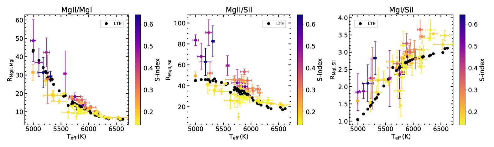
Figure 2: The line index ratios R of stars in Tab. LABEL:tab1 plotted as a function of their $T_{eff}$. The three subplots are for: Mg II/Mg I (left), Mg II/Si I (center) and Mg I/Si I (right). The colour map highlights the S-index dependence. The confidence bar for R values represents one standard deviation of the time variability of the single star. Black dots represent line index ratios obtained from the LTE synthesis.

3 Response Functions

We use the Response Function (RF) as a diagnostic to trace changes in temperature, together with theoretical (Kurucz, 1979) and semi-empirical models (Fontenla et al., 2011) of stellar atmospheres. The RF gives information about the first-order variations of the emergent intensity due to a perturbation of a given physical parameter (e.g. Mein, 1971; Beckers & Milkey, 1975; Caccin et al., 1977). In solar physics, response functions are widely employed to investigate spectral and spectro-polarimetric diagnostics (e.g. Cabrera Solana et al., 2005; Orozco Suárez & Del Toro Iniesta, 2007; Penza & Berrilli, 2014; Quintero Noda et al., 2017), for the characterization of filters (e.g. Penza et al., 2004; Fossum & Carlsson, 2005; Wachter, 2008; Ermolli et al., 2010), and are fundamental tools for spectro-polarimetric inversions (e.g. Ruiz Cobo & del Toro Iniesta, 1994; Milic & van Noor, 2017; Li et al., 2022; Ruiz Cobo et al., 2022). For the specific case of temperature perturbations, we have:

$$\delta I(\lambda)=\int_{0}^{\infty}RF(\lambda,\tau)\delta T(\tau)d\tau$$ (2)

where T is the temperature, $\lambda$ is the wavelength, and $\tau$ is the optical depth. We are interested in the response of the ratio of line indices that, after some algebra, can be written as:

$$RF_{ij}\approx\frac{RF_{core}^{(i)}}{I_{core}^{(i)}}-\frac{RF_{core}^{(j)}}{I_{core}^{(j)}}$$ (3)

where $R_{ij}$ is the ratio between the index of the i-line and the j-line ($R_{ij}=D_{i}/D_{j}$). The steps leading to Eq. 3 are detailed in Appendix B.

In order to compute the RFs to temperature variations, we employ the numerical approach described in Uitenbroek (2006) by considering different atmospheric models where the temperature profiles are perturbed only in a small interval of height (see also Criscuoli et al., 2013, 2023). Specifically, we computed the responses of line index ratios obtained perturbing the temperature of three Kurucz models having solar metallicity (log g = 4.5) and effective temperatures of 5000 K, 5777 K (Sun) and 6250 K. In order to test the goodness of the LTE approximation for computing lines that are typically treated in Non-LTE, the line syntheses, necessary to compute the line indices and their ratios in Eq. 3, were performed using both LTE and Non-LTE. For the Non-LTE syntheses we employed the Rybicki and Hummer (RH) code (Uitenbroek, 2001; Criscuoli, 2019), since SPECTRUM only allows computations in LTE. The Non-LTE synthesis of the Mg lines was performed using the 76-levels model atom described in Leenaarts et al. (2013a) and partial frequency redistribution (PRD); the synthesis of the Si I line was performed using a 15 levels plus continuum atom. We found that the response functions obtained with the two codes under the different assumptions are very similar. For simplicity, in Fig. 3 we show only the responses of the three indices obtained with RH in Non-LTE.

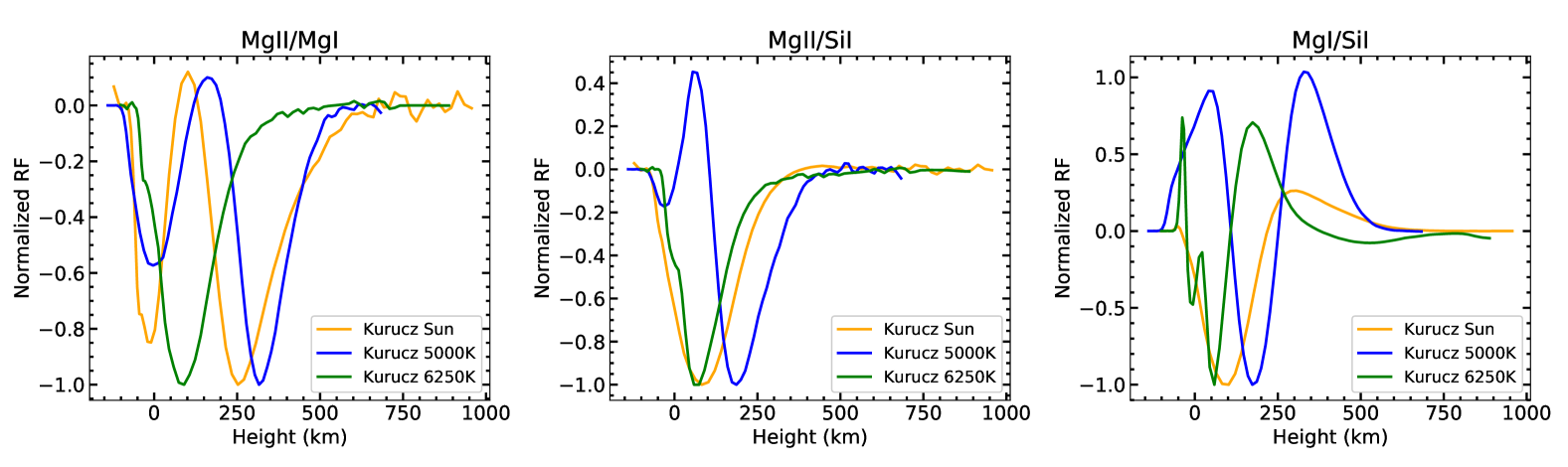
Figure 3: Comparison of the temperature response functions (RFs) normalized to their absolute maximum value, for the three index ratios computed in Non-LTE using the Kurucz solar model (orange line), a Kurucz model with $T_{eff}$ = 5000 K and log g = 4.5 (blue line), and a Kurucz model with $T_{eff}$ = 6250 K and log g = 4.5 (green line). For all three cases, we assumed the solar metallicity (i.e., [Fe/H]=0.00).

These plots provide two pieces of information:

• for all investigated atmosphere models, the three index ratios are sensitive to temperature variations up to a height (H) of about 600 km, H = 0 km corresponding to the base of the photosphere, where $\tau_{5000}=1$

• for all investigated atmosphere models, the response to the temperature of the index ratio Mg II/Mg I is almost always negative, meaning that for variations $\delta T>0$ the indices decrease; the response of the index ratio Mg II/Si I results negative everywhere in the solar and hotter models, while for colder atmospheres the response present also a positive lobe in the lower photosphere and that explains the change of the slope of synthetic relation in the central plot of Fig. 2 for $T_{eff}<5500K$. Finally, the response of the index ratio Mg I/Si I shows a greater dependence on the temperature of the model used. In particular, it presents negative and positive lobes with different relative weights for the three models, increasing the positive contribution for cooler stars that overcompensates the negative one. This explains the change of trend at T${}_{eff}>5700$ in the right panel of Fig. 2.

The different response of the ratios for these models indicates the need to assess the behavior of these lines as the temperature varies, taking into account the different atmospheric models. From this perspective, we note that the ratio between the two Mg lines behaves more consistently than other index ratios.

3.1 Photospheric or chromospheric indices?

The RFs shown in Fig. 3 are computed with Non-LTE spectral syntheses that use atmospheric models without temperature chromospheric rise; therefore, it is not surprising that they are consistent with results derived from LTE syntheses performed with SPECTRUM using the grid of the same models. However, we notice that the LTE syntheses obtained with the Kurucz models are also able to reproduce the experimental dependence of the index ratios on $T_{eff}$, particularly the Mg II/Mg I ratio. This result is not trivial, as these lines are individually used as indicators of chromospheric activity for single stars. Previous studies showed that collisions significantly influence the Mg II h and k line formation, making the peak intensities of the core of these lines sensitive to temperatures at their formation heights, which are chromospheric, as demonstrated in several works (e.g. Leenaarts et al., 2013a, b). To understand why indices derived from chromospheric lines can serve as proxies for photospheric temperature, we compared RFs computed in LTE using the Kurucz solar model with those obtained in Non-LTE from the quiet Sun model with a chromospheric rise (model 1001) by Fontenla et al. (2011) (FAL, hereafter). In both cases, computations are based on RH syntheses. The comparison between the RFs obtained with the Kurucz solar model in LTE and the FAL in Non-LTE is shown in Fig. 4.

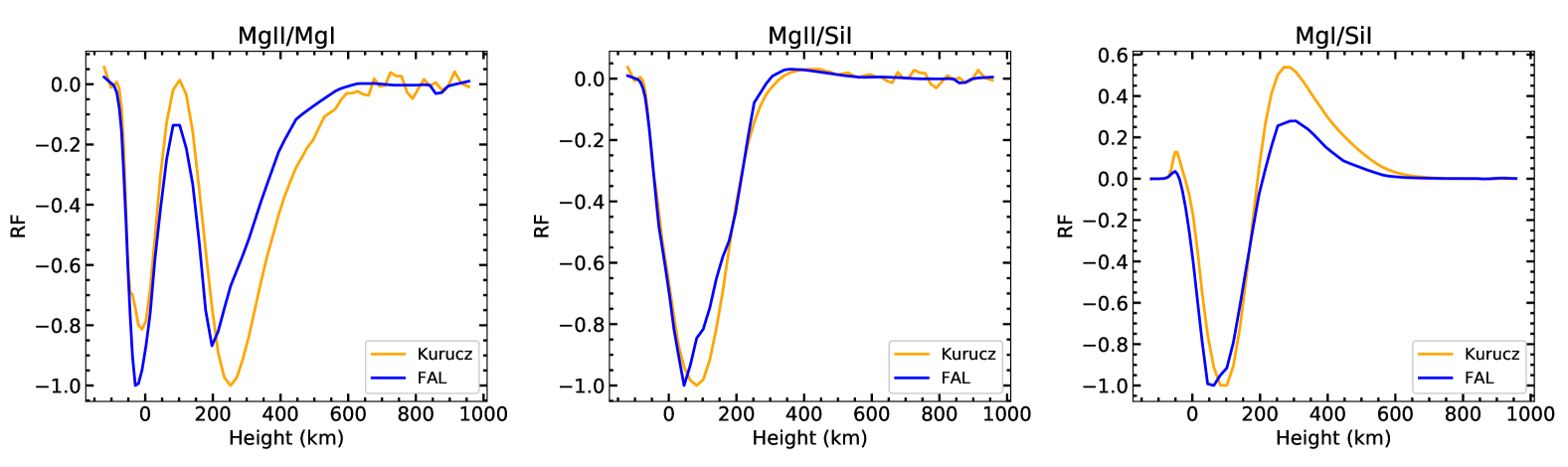
Figure 4: Comparison between the temperature RFs of the three index ratios computed by using the FAL model (blue line) and the Kurucz solar model (orange line).

Although some differences are noticed, especially for the Mg I/Si I ratio, our results clearly indicate that the response functions calculated with the Kurucz models in LTE provide a very good estimate of the temperature sensitivity of these ratios. Comparison of the RFs shown in Fig. 3 and Fig. 4 also confirms the good agreement between the LTE and Non-LTE approximations for the Kurucz solar model. To further understand why the presence of a chromosphere in the model seems to only marginally affect the shape of the RFs, we investigate the temperature RFs as a function of wavelength and height. We focus in particular on the spectral features of the Mg II h and k lines (illustrated in Fig. 5) and the cores of Si I and Mg I, whose corresponding RFs to temperature are shown in Fig. 6. The plots show that especially the individual peaks Mg II h and k (specifically h2v and k2v), and to a lesser extent, the Mg I and Si I cores, respond to temperature variations in the chromospheric layers. In particular, the Mg II line shows the maximum sensitivity of the h2 and k2 cores at a height of about 1000 km. The Mg I line core, on the other hand, has a primary maximum in the very lower photosphere, a secondary maximum around 500 km, and a much smaller one around 900 km. Finally, the Si I line presents two maxima, both in the photosphere, one at 300 km and a second at a height less than 100 km.

However, when we integrate the cores over the wavelength interval used to define the indices (right panel of Fig. 6), the resulting responses are predominantly photospheric. This occurs because, on one hand, the responses quickly become photospheric as we move away from the core, with regions such as the area between the h and k cores forming entirely in the photosphere (Uitenbroek, 1997). On the other hand, the cores of these lines form in Non-LTE conditions, which makes them less sensitive to local temperature variations (Leenaarts et al., 2013b).

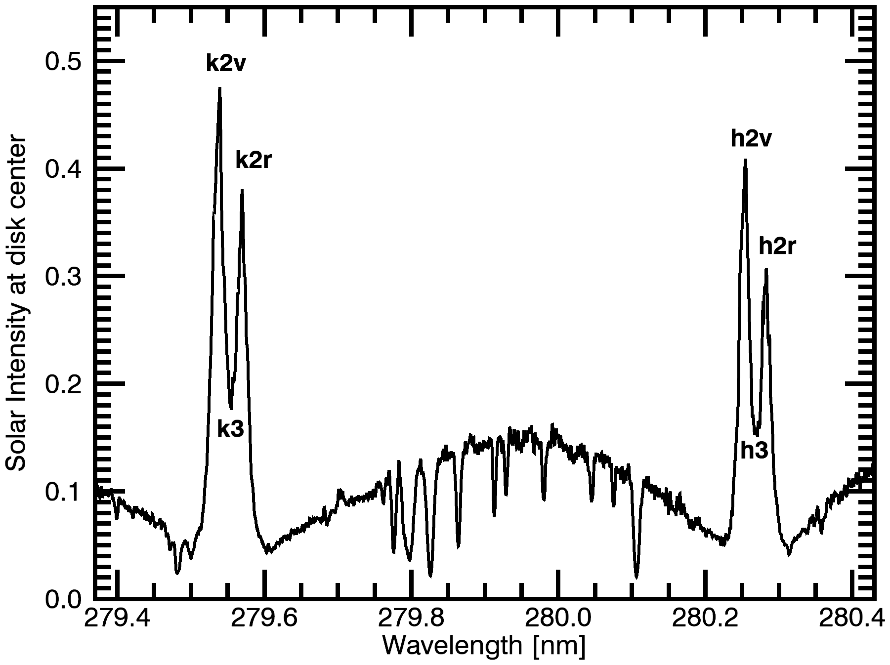
Figure 5: Hawaii UV atlas (Allen et al., 1977) disk center intensity of the solar spectrum around the Mg II h and k lines, normalized to the nearby continuum. According to conventional nomenclature, the central reversals are denoted with h3 and k3, the violet emission with h2v and k2v, and the red emission with h2r and k2r.

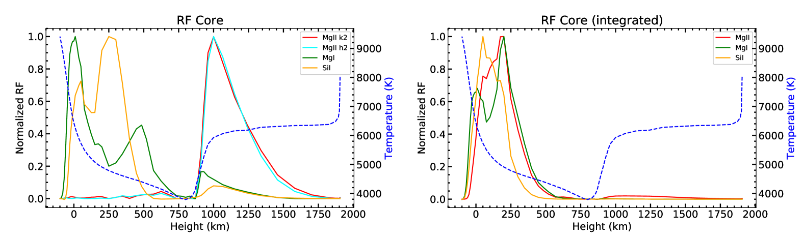
Figure 6: Left panel: Temperature Response Functions of the core intensity of the three lines, where for the Mg II h and k, we show the responses at the h2v and k2v peaks (see Fig. 5). Right panel: Temperature Response Functions of the intensity integrated over the spectral ranges indicated in Sec. 2. In both panels, the RFs are normalized to their maxima, while the dashed blue line represents the temperature stratification of the FAL model.

4 $T_{eff}$ determination by using the $MgII/MgI$ ratio

We found that the relation between the index ratio R = Mg II/Mg I and $T_{eff}$ can be described by a log-log relation:

$$log(T_{eff})=a\,log(R)+b$$ (4)

where the coefficients of the fit (black line in Figure 7), derived using the data in Fig. 2, are:

$$a=-0.126\pm 0.003\,\,\,\,\,(log(K))$$

$$b=3.907\pm 0.003\,\,\,\,\,(log(K))$$

The corresponding Pearson correlation coefficient of this correlation is r=-0.93. To estimate the statistical significance we performed a t-test and found (t = 17.2) there is a nonzero correlation at a confidence level greater than 99.9%. We note that the star that deviates the most from this fit is HD 166, that is a young and very active star.

Figure 7: Log-log fit between stellar $T_{eff}$ and line index ratio R = Mg II/Mg I. The red point represents the Sun.

In determining this relationship, we neglected the influence of gravity. In reality, the fit is derived from data that span a range of gravitational values. Furthermore, the Mg II/Mg I line ratio shows little variation for stars with effective temperatures above 5200 K, even within the gravity range of $4<\log g<5$.

To evaluate whether R=Mg II/Mg I is a good predictor of $T_{eff}$, we computed R for a separate sample of 35 solar-like stars (test-sample) and then applied the log-log relation above to estimate their effective temperatures. Unlike the stars in Tab. LABEL:tab1, this sample was obtained without requiring the presence of multiple spectra observed at different times. The properties of these 35 stars, as reported in the literature, are presented in Tab. LABEL:tab3 alongside our estimates of their effective temperatures ($T_{eff}^{\;\;\;\;(R)}$).

Table 3: List of the selected stars and their estimated effective temperature, based on the relation in Eq.4, labeled as $T_{eff}^{\;\;\;\;(R)}$. The other stellar parameters are obtained from the PASTEL and SIMBAD databases, as shown in Tab. LABEL:tab1. The B-V values with * are not derived by SIMBAD. Specifically: HD 25998, HD 78366 and HD 97334 by Pizzolato et al. (2003), HD 26293 by Boro Saikia et al. (2018). The stellar ages are from Takeda et al. (2007). $P_{rot}$ values are from Baliunas et al. (1996), Hempelmann et al. (2016) or Olspert et al. (2018), except for HD 9826 by Simpson et al. (2010). The S-index values with * are not derived by Mount Wilson database, but by Mittag et al. (2018).

STAR	$T_{eff}^{\;\;\;\;(R)}$	$T_{eff}$	B-V	log g	[$Fe/H$]	[$\alpha/Fe$]	Age	$P_{rot}$	S-index
HD	(K)	(K)		(dex)			(Gyr)	(days)
400	6110 $\pm$ 83	6173 $\pm$ 49	…	4.12 $\pm$ 0.07	-0.25 $\pm$ 0.07	0.30	$7.52^{+2.92}_{-3.32}$	…	0.151 $\pm$ 0.004
9826	6146 $\pm$ 82	6154 $\pm$ 70	0.540	4.16 $\pm$ 0.13	0.068 $\pm$ 0.091	0.19	$3.12^{+0.20}_{-0.24}$	7.3 $\pm$ 0.04	0.154 $\pm$ 0.005
10307	5978 $\pm$ 84	5888 $\pm$ 74	0.620	4.33 $\pm$ 0.08	0.032 $\pm$ 0.07	0.05	…	…	0.151 $\pm$ 0.003
16673	6128 $\pm$ 83	6265 $\pm$ 68	0.504	4.34 $\pm$ 0.08	-0.002 $\pm$ 0.055	0.22	…	5.98 $\pm$ 0.09	0.216 $\pm$ 0.008
22484	6055 $\pm$ 83	5993 $\pm$ 59	0.85	4.11 $\pm$ 0.15	-0.08 $\pm$ 0.06	0.09	$5.64^{+0.44}_{-1.72}$	…	0.146 $\pm$ 0.003
25998	6007 $\pm$ 84	6356 $\pm$ 160	0.52∗	4.56 $\pm$ 0.28	0.15 $\pm$ 0.18	0.28	…	2	0.286 $\pm$ 0.014
26923	5817 $\pm$ 86	5985 $\pm$ 69	…	4.45 $\pm$ 0.04	0.002 $\pm$ 0.06	0.18	…	10.6 $\pm$ 0.3	0.283 $\pm$ 0.012
27406	5911 $\pm$ 85	6109 $\pm$ 103	0.57∗	4.25 $\pm$ 0.11	0.12 $\pm$ 0.06	0.13	…	…	0.289 $\pm$ 0.001∗
27836	5936 $\pm$ 84	5760 $\pm$ 33	0.634	4.3	0.16	0.24	…	…	0.345 $\pm$ 0.011 ∗
27859	5595 $\pm$ 87	5891 $\pm$ 102	0.592	4.40 $\pm$ 0.08	0.12 $\pm$ 0.06	0.11	…	…	0.296 $\pm$ 0.012 ∗
28068	5659 $\pm$ 87	5757 $\pm$ 199	0.64	4.41 $\pm$ 0.08	0.07 $\pm$ 0.07	0.21	…	…	0.329 $\pm$ 0.032∗
28205	5985 $\pm$ 84	6220 $\pm$ 42	0.545	4.305 $\pm$ 0.005	0.142 $\pm$ 0.05	0.23	…	…	0.238 $\pm$ 0.002 ∗
28344	5682 $\pm$ 87	5921 $\pm$ 230	0.619	4.43 $\pm$ 0.06	0.13 $\pm$ 0.09	0.16	…	…	0.297 $\pm$ 0.020∗
28992	5345 $\pm$ 90	5882 $\pm$ 68	0.632	4.42 $\pm$ 0.10	0.14 $\pm$ 0.04	0.14	…	…	0.301 $\pm$ 0.007 ∗
33256	6563 $\pm$ 78	6376 $\pm$ 88	0.427	3.95 $\pm$ 0.18	-0.37 $\pm$ 0.11	0.16	…	…	0.153 $\pm$ 0.002
43042	6342 $\pm$ 80	6508 $\pm$ 59	…	4.26 $\pm$ 0.05	0.05 $\pm$ 0.05	0.13	$2.28^{+0.32}_{-0.36}$	…	0.163 $\pm$ 0.003
43318	6421 $\pm$ 79	6256 $\pm$ 60	0.50	3.88 $\pm$ 0.16	-0.17 $\pm$ 0.05	0.17	…	…	…
48682	6062 $\pm$ 83	6052 $\pm$ 125	…	4.35 $\pm$ 0.19	0.11 $\pm$ 0.04	0.14	$4.00^{+3.20}_{-0.92}$	…	0.151 $\pm$ 0.004
76932	6150 $\pm$ 82	5869 $\pm$ 69	0.53	4.04 $\pm$ 0.23	-0.91 $\pm$ 0.09	…	…	…	…
78366	5869 $\pm$ 85	5995 $\pm$ 41	0.60	4.50 $\pm$ 0.1	0.04 $\pm$ 0.03	0.16	$0.00^{+0.68}_{-0.00}$	9.52 $\pm$ 0.08	0.245 $\pm$ 0.019
82885	5453 $\pm$ 89	5508 $\pm$ 95	0.77	4.44 $\pm$ 0.13	0.31 $\pm$ 0.09	-0.03	…	17.88 $\pm$ 0.18	0.288 $\pm$ 0.025
84737	5897 $\pm$ 85	5896 $\pm$ 46	0.62	4.13 $\pm$ 0.11	0.093 $\pm$ 0.06	0.07	$4.08^{+0.36}_{-0.28}$	4.30 $\pm$ 0.02	0.136 $\pm$ 0.004
89449	6298 $\pm$ 80	6472 $\pm$ 55	…	4.13 $\pm$ 0.01	0.11 $\pm$ 0.01	0.22	…	…	0.414 $\pm$ 0.015
97334	5691 $\pm$ 87	5867 $\pm$ 52	0.60	4.36 $\pm$ 0.10	0.05 $\pm$ 0.03	0.18	$0.00^{+2.92}_{-0.00}$	7.93 $\pm$ 0.05	0.333 $\pm$ 0.017
101501	5403 $\pm$ 89	5465 $\pm$ 155	0.74	4.54 $\pm$ 0.05	-0.06 $\pm$ 0.09	0.07	11.32	15.9 $\pm$ 0.2	0.303 $\pm$ 0.024
103095	5389 $\pm$ 89	5052 $\pm$ 70	0.75	4.57 $\pm$ 0.24	-1.34 $\pm$ 0.12	0. 58	$0.00^{+2.44}_{-0.00}$	34.03 $\pm$ 0.68	0.184 $\pm$ 0.011
106516	6220 $\pm$ 82	6157 $\pm$ 175	0.46	4.36 $\pm$ 0.20	-0.70 $\pm$ 0.19	…	…	6.63 $\pm$ 0.04	0.208 $\pm$ 0.008
114378	6295 $\pm$ 81	6382 $\pm$ 25	0.572	4.18 $\pm$ 0.11	-0.19 $\pm$ 0.06	…	…	4.39 $\pm$ 0.02	0.241 $\pm$ 0.007
115043	5629 $\pm$ 87	5749 $\pm$ 260	0.61	4.47	-0.06 $\pm$ 0.05	0.23	…	5.5 $\pm$ 0.1	0.321 $\pm$ 0.018
120136	6200 $\pm$ 82	6479 $\pm$ 110	0.49	4.32 $\pm$ 0.25	0.28 $\pm$ 0.10	0.30	$1.64^{+0.44}_{-0.52}$	3.07 $\pm$ 0.06	0.188 $\pm$ 0.006
141004	5906 $\pm$ 85	5908 $\pm$ 76	0.61	4.17 $\pm$ 0.10	-0.007 $\pm$ 0.050	0.14	$6.32^{+0.88}_{-1.56}$	26	0.156 $\pm$ 0.006
152391	5370 $\pm$ 89	5452 $\pm$ 46	0.76	4.49 $\pm$ 0.09	-0.03 $\pm$ 0.07	0.12	…	10.62 $\pm$ 0.13	0.391 $\pm$ 0.036
185144	5554 $\pm$ 88	5289 $\pm$ 90	0.78	4.49 $\pm$ 0.13	-0.22 $\pm$ 0.10	0.03	…	27.7 $\pm$ 0.8	0.218 $\pm$ 0.020
217014	5787 $\pm$ 86	5766 $\pm$ 59	0.7	4.31 $\pm$ 0.14	0.18 $\pm$ 0.06	0.03	$6.76^{+1.64}_{-1.48}$	38.0 $\pm$ 0.6	0.149 $\pm$ 0.004
284253	5393 $\pm$ 89	5331 $\pm$ 93	0.81	4.505 $\pm$ 0.009	0.12 $\pm$ 0.02	0.04	…	…	0.412 $\pm$ 0.016 ∗
(To be continued)

In Fig. 8 we plot our effective temperature determinations ($T_{eff}^{\;\;\;\;(R)}$) versus the average values from the literature ($T_{eff}$), highlighting their dependence on $\log g$, S-index and metallicity using a color coding. Except for a few stars in the sample, the effective temperature determinations appear to agree with the values reported in the literature. To quantify this agreement, we performed a Wilcoxon signed-rank test. The Wilcoxon signed-rank test is a non-parametric statistical method used for hypothesis testing. It is applied either to evaluate the location of a population based on a sample of data or to compare the locations of two populations using two matched samples. For the sample of stars shown in Fig. 8, the test statistic ($W$) is calculated as $W$=210. This value is compared to the critical value from the Wilcoxon Signed-Rank Test Critical Values Table (two-tailed) corresponding to $n$ = 35 (the number of stars in the sample) and $\alpha$ =0.05 (95% confidence level). The critical value for these parameters is 195. Since the calculated $W$ (210) is greater than the critical value (195), we conclude that there is no significant difference between the two population medians at the 95% confidence level. That is, our results are in good agreement with previous studies.

The reliability of the empirically derived log-log relation to estimate the effective temperature will be examined further in the next section.

Figure 8: The effective temperatures obtained in this work ($T_{eff}^{\;\;\;\;(R)}$, y-axis), for the stars in Tab. LABEL:tab3, against the literature values (x-axis). In all panels the dashed black line indicates the bisector, while the color map shows the dependence on log g (top panel), S-index (middle panel) and [Fe/H] (bottom panel).

5 Discussion and conclusions

In this study, we examined the dependence of the ratios of core-to-wing indices on stellar parameters, focusing on three mid-UV lines: Mg II 280.0 nm, Mg I 285.2 nm, and Si I 288.16 nm. We analyzed spectra from 52 solar-like stars in the IUE database and explored how the derived line index ratios relate to stellar fundamental parameters. Our findings reveal a strong dependence on effective temperature and a secondary dependence on gravity, suggesting that the UV line index ratios investigated here are effective indicators of photospheric temperatures. Among the indices examined, the Mg II/Mg I ratio exhibits the least scatter and the clearest trend with effective temperature. Furthermore, this ratio shows the best agreement with LTE synthesis based on Kurucz’s atmospheric models for solar-like stars, making it the most reliable indicator of photospheric conditions.

To gain insight into our findings, we investigated the RFs to temperature perturbations applied to models with and without a chromosphere. We confirm the chromospheric sensitivity of the individual peaks Mg II h and k, while the cores of Mg I and Si I are more sensitive to temperature perturbations at lower heights in the atmosphere. However, we showed that the responses of the cores of the three lines shift toward the photosphere when integrating over the wavelength ranges used to define the indices described in Tab. 2. Consequently, also the line indices derived from the three lines and their ratios show the highest sensitivity to temperature perturbations in the photosphere. This result aligns with results previously found for the Ca II H and K lines, whose cores form in the chromosphere, but whose responses become photospheric when observed with broadband filters (Ermolli et al., 2010; Murabito et al., 2023) typically employed for monitoring solar activity. However, the line ratios we considered exhibit different responses to temperature variations. Specifically, Mg II/Mg I and Mg II/Si I decrease with positive temperature perturbations, whereas Mg I/Si I shows the opposite trend. In Sec. 3.1 we showed that the exact sign, shape, and amplitude of the RFs of the line indices and their ratios depend on the atmosphere model; however, responses obtained in Non-LTE using an atmosphere with a chromosphere are well matched by responses obtained using LTE approximation with models without a chromosphere.

Supported by the results obtained from the analysis of synthetic spectra, which indicate that all the analyzed index ratios are sensitive to photospheric perturbations, we derived an empirical log-log relation between the observed index ratio Mg II/Mg I and T_eff, and used this relation to estimate the effective temperature of a second sample of 35 solar-like stars (test-sample) from the IUE database. We found that the estimated temperatures agree with the ones provided in the literature at a 95% confidence level.

However, examining the plots in Fig. 8, it is clear that the effective temperatures derived from Eq. 4 tend to be slightly underestimated for stars with high magnetic activity. Indeed, all stars listed in Tab. LABEL:tab3 with an S-index $\gtrsim$ 0.22 exhibit $T_{eff}$ estimates lower than those in the literature. This discrepancy may stem from the use of a single spectrum, which could have led to higher R values than the average, thereby underestimating $T_{eff}$. On the other hand, low metallicity appears to significantly contribute to overestimating $T_{eff}$. A notable example is HD 103095, an extremely metal-poor star ([Fe/H] $\simeq$ -1.34), which shows the largest $T_{eff}$ overestimation. Additionally, the results in the top panel of Fig. 8 suggest that for stars with surface gravity values log g $\lesssim$ 4.0 or log g $\gtrsim$ 4.5 the proposed method will most likely provide $T_{eff}$ estimates that deviate from values reported in the literature. The use of line depth ratios as $T_{eff}$ calibrators is already well established, but so far it has been mostly limited to lines in the visible and infrared ranges. Here, we demonstrate that it is possible to extend this approach to the mid-UV range, with the advantage of using the same lines as diagnostics of stellar chromospheres and stellar fundamental parameters. In particular, Fig. 6 illustrates how different atmospheric heights are sampled depending on the width of the spectral range of integration around the line cores. The capability to investigate the height dependence of temperature, from the photosphere to the upper chromosphere, using the same spectral line, exists by progressively refining the core selection. This approach will be the focus of a future study. Another possible extension of this work could involve new calibrations using stellar data from other UV spectral observations, such as those from SOLSTICE (Snow et al., 2013), Hubble Space Telescope (e.g. Sahu et al., 2023), FUSE and CUTE, as well as from future instruments such as MAUVE, HWO and MANTIS. However, in the context of UV spectroscopy, the game changer appears to be UVEX(Kulkarni et al., 2021), the new NASA Medium Explorer mission to explore the ultraviolet sky, which is planned to be launched in 2030. Indeed, this satellite will cover the entire sky simultaneously in the FUV and in the NUV bands. This means a unique opportunity to use UV spectral diagnostics to investigate a wide range of young and old stellar tracers in the Milky Way and in nearby stellar systems (globulars, dwarf galaxies).

In light of this, our next objectives are twofold: first, to analyze the behavior of the studied lines in the context of solar variability, and second, to extend the approach by incorporating different pairs of UV lines for M-type stars. This is particularly important because M dwarfs are key targets in the search for exoplanets due to their abundance, favorable conditions for detecting transiting planets, and the significant impact of their activity on planetary habitability. The applicability of the method presented in this work to stars significantly different from the Sun, in terms of gravity, abundance, or high magnetic activity, will require a more detailed investigation. This should be done by exploring different atmospheric models and analyzing additional data to assess the effect of such conditions on these spectral lines.

6 Appendix A

We report here the color maps showing the dependence of the line index ratios Mg II/Mg I, Mg II/Si I and Mg I/Si I on log g (Fig. 9) and [Fe/H] (Fig. 10). These figures are the same as in Fig. 2, except for the different color-coded dependence.

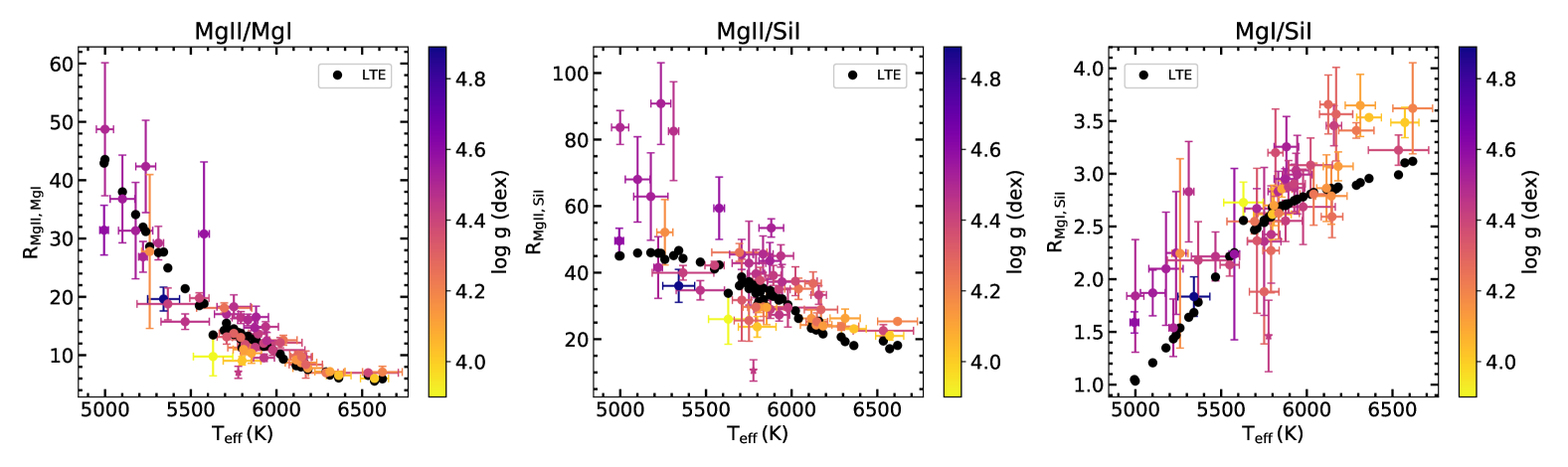
Figure 9: Same as Fig 2, but with the color map highlighting the log g dependence.

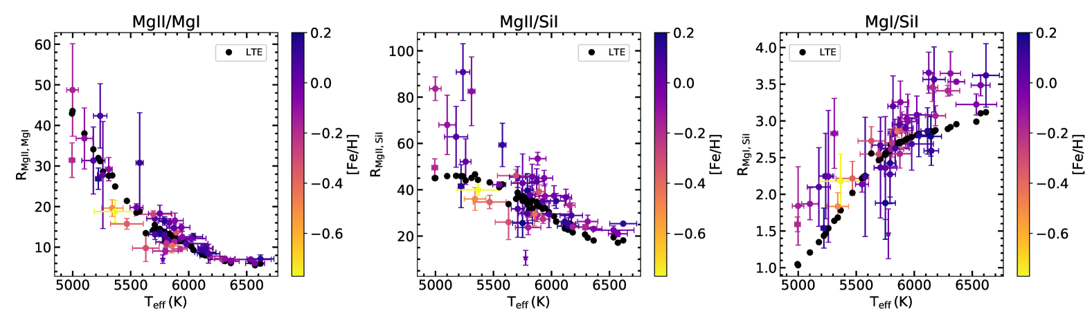
Figure 10: Same as Fig. 2, but with the colour map highlighting the [Fe/H] dependence.

7 Appendix B

We detail here the algebraic steps that lead to the final expression of the Response Function of the line index ratios reported in Eq. 3. To simplify the notation, we omit the dependencies on $\lambda$ and $\tau$, so we can write the variations for D as:

$$\frac{\delta D}{D}=\frac{\delta I_{core}}{I_{core}}-\frac{\delta I_{cont}}{I_{cont}}=\frac{\int_{0}^{\infty}RF_{core}\delta Td\tau}{I_{core}}-\frac{\int_{0}^{\infty}RF_{cont}\delta Td\tau}{I_{cont}}=\frac{\int_{0}^{\infty}(RF_{core}-D^{.}RF_{cont})\delta Td\tau}{I_{core}}$$ (5)

Then, the Response Function for the single line index D results:

$$RF_{D}=\frac{D}{I_{core}}(RF_{core}-DRF_{cont})$$ (6)

In analogous way, variations of the ratio ($R_{ij}\equiv D_{i}/D_{j}$) of two different indices $i,j$ result:

$$\frac{\delta R_{ij}}{R_{ij}}=\frac{\delta D_{i}}{D_{i}}-\frac{\delta D_{j}}{D_{j}}=\frac{\int_{0}^{\infty}(RF_{D_{i}}-R_{ij}^{.}RF_{D_{j}})\delta Td\tau}{D_{1}}$$ (7)

With simple algebraic passages, we obtain:

$$\frac{\delta R_{ij}}{R_{ij}}=\int_{0}^{\infty}\left[\frac{RF_{core}^{(i)}}{I_{core}^{(i)}}-\frac{RF_{cont}^{(i)}}{I_{cont}^{(i)}}-\frac{RF_{core}^{(j)}}{I_{core}^{(j)}}+\frac{RF_{cont}^{(j)}}{I_{cont}^{(j)}}\right]\delta Td\tau$$ (8)

Because the spectral lines are very close to each other, we can assume that the continuum intensities and their response functions are the same, so that the relation above can be rewritten as:

$$\frac{\delta R_{ij}}{R_{ij}}\approx\int_{0}^{\infty}\left[\frac{RF_{core}^{(i)}}{I_{core}^{(i)}}-\frac{RF_{core}^{(j)}}{I_{core}^{(j)}}\right]\delta Td\tau$$ (9)

References

- Afşar et al. (2023) Afşar, M., Bozkurt, Z., Topcu, G. B., et al. 2023, ApJ, 949, 86, doi: 10.3847/1538-4357/acc946
- Allen et al. (1977) Allen, M. S., McAllister, H. C., & Jefferies, J. T. 1977, High resolution atlas of the solar spectrum 2678-2931 A
- Alonso et al. (1996) Alonso, A., Arribas, S., & Martinez-Roger, C. 1996, A&A, 313, 873
- Anders & Grevesse (1989) Anders, E., & Grevesse, N. 1989, Geochim. Cosmochim. Acta, 53, 197, doi: 10.1016/0016-7037(89)90286-X
- Asplund et al. (2009) Asplund, M., Grevesse, N., Sauval, A. J., & Scott, P. 2009, ARA&A, 47, 481, doi: 10.1146/annurev.astro.46.060407.145222
- Baliunas et al. (1996) Baliunas, S., Sokoloff, D., & Soon, W. 1996, ApJ, 457, L99, doi: 10.1086/309891
- Basturk et al. (2011) Basturk, O., Dall, T., Collet, R., Lo Curto, G., & Selam, S. 2011, A&A, 535, A17, doi: 10.1051/0004-6361/201117740
- Beckers & Milkey (1975) Beckers, J. M., & Milkey, R. W. 1975, Sol. Phys., 43, 289, doi: 10.1007/BF00152353
- Berrilli et al. (2020) Berrilli, F., Criscuoli, S., Penza, V., & Lovric, M. 2020, Sol. Phys., 295, 38, doi: 10.1007/s11207-020-01603-5
- Bertello et al. (2016) Bertello, L., Pevtsov, A., Tlatov, A., & Singh, J. 2016, Sol. Phys., 291, 2967, doi: 10.1007/s11207-016-0927-9
- Biazzo et al. (2007) Biazzo, K., Frasca, A., Catalano, S., & Marilli, E. 2007, Astronomische Nachrichten, 328, 938, doi: 10.1002/asna.20071078110.1002/asna.200610781
- Bono et al. (2024) Bono, G., Braga, V. F., & Pietrinferni, A. 2024, A&A Rev., 32, 4, doi: 10.1007/s00159-024-00153-0
- Bordi et al. (2015) Bordi, I., Berrilli, F., & Pietropaolo, E. 2015, Annales Geophysicae, 33, 267, doi: 10.5194/angeo-33-267-2015
- Boro Saikia et al. (2018) Boro Saikia, S., Marvin, C., Jeffers, S., et al. 2018, A&A, 616, A108, doi: https://doi.org/10.1051/0004-6361/201629518
- Brandenburg & Giampapa (2018) Brandenburg, A., & Giampapa, M. 2018, Astrophysical Journal Letters, 855, L22, doi: 10.3847/2041-8213
- Brandenburg et al. (2017) Brandenburg, A., Mathur, S., & Metcalfe, T. S. 2017, ApJ, 845, 79, doi: 10.3847/1538-4357/aa7cfa
- Buccino & Mauas (2008) Buccino, A., & Mauas, P. 2008, A&A, 483, 903
- Cabrera Solana et al. (2005) Cabrera Solana, D., Bellot Rubio, L. R., & del Toro Iniesta, J. C. 2005, A&A, 439, 687, doi: 10.1051/0004-6361:20052720
- Caccin et al. (1977) Caccin, B., M.T., G., Marmolino, C., & Severino, G. 1977, å, 54, 227
- Caccin et al. (2002) Caccin, B., Penza, V., & M.T., G. 2002, å, 386, 286, doi: 10.1051/0004-6361:20020217
- Casagrande et al. (2021) Casagrande, L., Lin, J., Rains, A. D., et al. 2021, MNRAS, 507, 2684, doi: 10.1093/mnras/stab2304
- Cayrel & Cayrel (1963) Cayrel, G., & Cayrel, R. 1963, ApJ, 137, 431, doi: 10.1086/147521
- Choi et al. (2015) Choi, H., Lee, J., Suyeon, O., et al. 2015, AJ, 802, 67, doi: http://dx.doi.org/10.1088/0004-637X/802/1/67
- Criscuoli (2019) Criscuoli, S. 2019, ApJ, 872, 52, doi: 10.3847/1538-4357/aaf6b7
- Criscuoli et al. (2013) Criscuoli, S., Ermolli, I., Uitenbroek, H., & Giorgi, F. 2013, ApJ, 763, 144, doi: 10.1088/0004-637X/763/2/144
- Criscuoli et al. (2023) Criscuoli, S., Marchenko, S., DeLand, M., Choudhary, D., & Kopp, G. 2023, ApJ, 951, 151, doi: 10.3847/1538-4357/acd17d
- Criscuoli et al. (2018) Criscuoli, S., Penza, V., Lovric, M., & Berrilli, F. 2018, ApJ, 865, 22, doi: 10.3847/1538-4357/aad809
- da Silva Santos et al. (2020) da Silva Santos, J. M., de la Cruz Rodríguez, J., Leenaarts, J., et al. 2020, A&A, 634, A56, doi: 10.1051/0004-6361/201937117
- De Pontieu et al. (2014) De Pontieu, B., Title, A. M., Lemen, J. R., et al. 2014, Sol. Phys., 289, 2733, doi: 10.1007/s11207-014-0485-y
- DeLand & Marchenko (2013) DeLand, M., & Marchenko, S. 2013, J. Geophys Res. Atmos, 118, 3415–3423, doi: doi:10.1002/jgrd.50310
- Di Mauro et al. (2022) Di Mauro, M. P., Reda, R., Mathur, S., et al. 2022, ApJ, 940, 93, doi: 10.3847/1538-4357/ac8f44
- Egan et al. (2018) Egan, A., Fleming, B., France, K., et al. 2018, Proc of SPIE 10699
- Egeland et al. (2017) Egeland, R., Soon, W., Baliunas, S., et al. 2017, ApJ, 835, 25, doi: 10.3847/1538-4357/835/1/25
- Ermolli et al. (2003) Ermolli, I., Berrilli, F., & Florio, A. 2003, A&A, 412, 857, doi: 10.1051/0004-6361:20031479
- Ermolli et al. (2010) Ermolli, I., Criscuoli, S., Uitenbroek, H., et al. 2010, A&A, 523, A55, doi: 10.1051/0004-6361/201014762
- Ermolli et al. (2013) Ermolli, I., Matthes, K., Dudok de Wit, T., et al. 2013, Atmospheric Chemistry & Physics, 13, 3945, doi: 10.5194/acp-13-3945-201310.5194/acpd-12-24557-2012
- Fanelli et al. (1990) Fanelli, M., O’ Connell, R., Burstein, D., & Wu, C. 1990, ApJ, 364, 272, doi: 10.1086/169411
- Fontenla et al. (2011) Fontenla, J. M., Harder, J., Livingston, W., Snow, M., & Woods, T. 2011, Journal of Geophysical Research (Atmospheres), 116, D20108, doi: 10.1029/2011JD016032
- Fossum & Carlsson (2005) Fossum, A., & Carlsson, M. 2005, ApJ, 625, 556, doi: 10.1086/429614
- Fuhrmann & Chini (2018) Fuhrmann, K., & Chini, R. 2018, ApJ, 858, 103, doi: 10.3847/1538-4357/aabaff
- Fukue et al. (2015) Fukue, K., Matsunaga, N., Yamamoto, R., et al. 2015, ApJ, 812, 64, doi: 10.1088/0004-637X/812/1/64
- Gaidos et al. (2000) Gaidos, E. J., Henry, G. W., & Henry, S. M. 2000, AJ, 120, 1006, doi: 10.1086/301488
- Gehren (1981) Gehren, T. 1981, A&A, 100, 97
- Gray & Johanson (1991) Gray, D., & Johanson, H. 1991, PASP, 103, 439, doi: 10.1086/132839
- Gray & Corbally (1994) Gray, R., & Corbally, C. 1994, AJ, 107, 742, doi: 10.1086/116893
- Heath & Schlesinger (1986) Heath, D., & Schlesinger, B. 1986, Journal of Geophysical Research, 91, 8672, doi: https://doi.org/10.1029/JD091iD08p08672
- Hempelmann et al. (2016) Hempelmann, A., Mittag, M., Gonzalez-Perez, J. N., et al. 2016, A&A, 586, A14, doi: 10.1051/0004-6361/201526972
- Hillier (2020) Hillier, D. J. 2020, Galaxies, 8, 60, doi: 10.3390/galaxies8030060
- Houdebine et al. (1996) Houdebine, E. R., Mathioudakis, M., Doyle, J. G., & Foing, B. H. 1996, A&A, 305, 209
- Hussain et al. (2016) Hussain, G., Alvarado-Gómez, J., Grunhut, J., et al. 2016, A&A, 585, A77, doi: 10.1051/0004-6361/201526595
- Indahl et al. (2024) Indahl, B. L., Fleming, B., France, K., et al. 2024, in Space Telescopes and Instrumentation 2024: Ultraviolet to Gamma Ray, ed. J.-W. A. den Herder, S. Nikzad, & K. Nakazawa, Vol. 13093, International Society for Optics and Photonics (SPIE), 130930B, doi: 10.1117/12.3020386
- Jejčič et al. (2022) Jejčič, S., Heinzel, P., Schmieder, B., et al. 2022, ApJ, 932, 3, doi: 10.3847/1538-4357/ac6bf5
- Jian et al. (2019) Jian, M., Matsunaga, N., & Fukue, K. 2019, MNRAS, 485, 1310, doi: https://doi.org/10.1093/mnras/stz237
- Kim et al. (2022) Kim, D., Choi, H., & Yi, Y. 2022, Journal of the Korean Astronomical Society, 55, 59
- Kovtyukh et al. (2023) Kovtyukh, V., Lemasle, B., Nardetto, N., et al. 2023, MNRAS, 523, 5047, doi: 10.1093/mnras/stad1708
- Kovtyukh et al. (2006) Kovtyukh, V. V., Soubiran, C., Bienaymé, O., Mishenina, T. V., & Belik, S. I. 2006, MNRAS, 371, 879, doi: 10.1111/j.1365-2966.2006.10719.x
- Kulkarni et al. (2021) Kulkarni, S. R., Harrison, F. A., Grefenstette, B. W., et al. 2021, arXiv e-prints, arXiv:2111.15608, doi: 10.48550/arXiv.2111.15608
- Kurucz (1979) Kurucz, R. L. 1979, ApJS, 40, 1, doi: 10.1086/190589
- Landi Degl’Innocenti & Landi Degl’Innocenti (1977) Landi Degl’Innocenti, E., & Landi Degl’Innocenti, M. 1977, å, 56, 111
- Leenaarts et al. (2013a) Leenaarts, J., Pereira, T. M. D., Carlsson, M., Uitenbroek, H., & De Pontieu, B. 2013a, ApJ, 772, 90, doi: 10.1088/0004-637X/772/2/90
- Leenaarts et al. (2013b) —. 2013b, ApJ, 772, 89, doi: 10.1088/0004-637X/772/2/89
- Li et al. (2022) Li, H., del Pino Alemán, T., Trujillo Bueno, J., & Casini, R. 2022, ApJ, 933, 145, doi: 10.3847/1538-4357/ac745c
- Lind et al. (2012) Lind, K., Bergemann, M., & Asplund, M. 2012, MNRAS, 427, 50, doi: 10.1111/j.1365-2966.2012.21686.x
- Linsky (2017) Linsky, J. L. 2017, ARA&A, 55, 159, doi: 10.1146/annurev-astro-091916-055327
- Lovric et al. (2017) Lovric, M., Tosone, F., Pietropaolo, E., et al. 2017, Journal of Space Weather and Space Climate, 7, A6, doi: 10.1051/swsc/2017001
- Loyd et al. (2021) Loyd, R. O. P., Shkolnik, E. L., Schneider, A. C., et al. 2021, ApJ, 907, 91, doi: 10.3847/1538-4357/abd0f0
- Majidi et al. (2024) Majidi, F., Saba, A., Bradley, L., et al. 2024, AAS/Division for Planetary Sciences Meeting Abstracts
- Mascareno et al. (2015) Mascareno, A., Rebolo, R., Gonzalez Hernandex J.I., D., & Esposito, M. 2015, MNRAS, 452, 2745, doi: https://doi.org/10.1093/mnras/stv1441
- Matsunaga et al. (2021) Matsunaga, N., Jian, M., Taniguchi, D., & Elgueta, S. 2021, MNRAS, 506, 1031, doi: https://doi.org/10.1093/mnras/stab1770
- Mayor et al. (2004) Mayor, M., Udry, S., Naef, D., et al. 2004, A&A, 415, 391, doi: 10.1051/0004-6361:20034250
- Mein (1971) Mein, P. 1971, Sol. Phys., 20, 3, doi: 10.1007/BF00146089
- Meléndez et al. (2014) Meléndez, J., Ramírez, I., Karakas, A. I., et al. 2014, ApJ, 791, 14, doi: 10.1088/0004-637X/791/1/14
- Metcalfe et al. (2024) Metcalfe, T. S., van Saders, J. L., Huber, D., et al. 2024, ApJ, 974, 31, doi: 10.3847/1538-4357/ad6dd6
- Milic & van Noor (2017) Milic, I., & van Noor, M. 2017, å, 601, 100, doi: 10.1051/0004-6361/201629980
- Mittag et al. (2018) Mittag, M., Schmitt, J., & schröder, K. 2018, A&A, 618, A48, doi: 10.1051/0004-6361/201833498
- Mittag et al. (2023) Mittag, M., Schmitt, J. H. M. M., & Schröder, K. P. 2023, A&A, 674, A116, doi: 10.1051/0004-6361/202245060
- Morrill et al. (2001) Morrill, J., Dere, K., & Korendyke, C. 2001, ApJ, 557, 854, doi: 10.1086/321683
- Murabito et al. (2023) Murabito, M., Ermolli, I., Chatzistergos, T., et al. 2023, ApJ, 947, 18, doi: 10.3847/1538-4357/acc529
- National Academies of Sciences, Engineering & Medicine (2021) National Academies of Sciences, Engineering & Medicine. 2021, Pathways to Discovery in Astronomy and Astrophysics for the 2020s, doi: 10.17226/26141
- Olspert et al. (2018) Olspert, N., Lehtinen, J. J., Käpylä, M. J., Pelt, J., & Grigorievskiy, A. 2018, A&A, 619, A6, doi: 10.1051/0004-6361/201732525
- Orozco Suárez & Del Toro Iniesta (2007) Orozco Suárez, D., & Del Toro Iniesta, J. C. 2007, A&A, 462, 1137, doi: 10.1051/0004-6361:20066201
- Penza & Berrilli (2014) Penza, V., & Berrilli, F. 2014, Sol. Phys., 289, 27, doi: 10.1007/s11207-013-0340-6
- Penza et al. (2004) Penza, V., Caccin, B., & Del Moro, D. 2004, A&A, 427, 345, doi: 10.1051/0004-6361:20041151
- Pepe et al. (2011) Pepe, F., Lovis, C., Ségransan, D., et al. 2011, A&A, 534, A58, doi: 10.1051/0004-6361/201117055
- Peralta et al. (2022) Peralta, J. I., Vieytes, M. C., Mendez, A. M. P., & Mitnik, D. M. 2022, A&A, 657, A108, doi: 10.1051/0004-6361/202141973
- Peralta et al. (2023) —. 2023, A&A, 676, A18, doi: 10.1051/0004-6361/202346156
- Pizzolato et al. (2003) Pizzolato, N., Maggio, A., Sciortino, S., & Ventura, P. 2003, A&A, 397, 147, doi: DOI: 10.1051/0004-6361:20021560
- Quintero Noda et al. (2017) Quintero Noda, C., Shimizu, T., Katsukawa, Y., et al. 2017, MNRAS, 464, 4534, doi: 10.1093/mnras/stw2738
- Radick & Pevtsov (2018) Radick, R., & Pevtsov, A. 2018, HK Project v1995 NSO, 1.0, Zenodo, doi: 10.5281/zenodo.15991
- Recio-Blanco et al. (2023) Recio-Blanco, A., de Laverny, P., Palicio, P. A., et al. 2023, A&A, 674, A29, doi: 10.1051/0004-6361/202243750
- Reda & Penza (2024) Reda, R., & Penza, V. 2024, in Memorie della Società Astronomica Italiana, Vol. 95, 12th Young Researcher Meeting, ed. R. D’Agostino, A. Baldi, P. Cacciotto, D. Pietrobon, & E. Preziosi, 46–50, doi: 10.36116/MEMSAIT_95N1.2024.46
- Reda et al. (2023) Reda, R., Giovannelli, L., Alberti, T., et al. 2023, MNRAS, 519, 6088, doi: 10.1093/mnras/stac3825
- Ruiz Cobo & del Toro Iniesta (1994) Ruiz Cobo, B., & del Toro Iniesta, J. 1994, å, 283, 129
- Ruiz Cobo et al. (2022) Ruiz Cobo, B., Quintero Noda, C., Gafeira, R., et al. 2022, A&A, 660, A37, doi: 10.1051/0004-6361/202140877
- Saar & Brandenburg (1999) Saar, S. H., & Brandenburg, A. 1999, ApJ, 524, 295, doi: 10.1086/307794
- Sahu et al. (2023) Sahu, S., Gansicke, B., Tremblay, P., et al. 2023, MNRAS, 526, 5800, doi: https://doi.org/10.1093/mnras/stad2663
- Sainz Dalda et al. (2019) Sainz Dalda, A., de la Cruz Rodríguez, J., De Pontieu, B., & Gošić, M. 2019, ApJ, 875, L18, doi: 10.3847/2041-8213/ab15d9
- Sanz-Forcada et al. (2010) Sanz-Forcada, J., Ribas, I., Micela, G., et al. 2010, A&A, 511, L8, doi: 10.1051/0004-6361/200913670
- Schrijver et al. (1992) Schrijver, C. J., Dobson, A. K., & Radick, R. R. 1992, å, 258, 432
- Schröder (2008) Schröder, C. 2008, PhD Thesis, University of Hamburg
- Simpson et al. (2010) Simpson, E. K., Baliunas, S. L., Henry, G. W., & Watson, C. A. 2010, MNRAS, 408, 1666, doi: 10.1111/j.1365-2966.2010.17230.x
- Snow et al. (2013) Snow, M., Reberac, A., Quemerais, E., McClintock, W., & Woods, T. 2013, New Catalog of Ultraviolet Stellar Spectra for Calibration, Tech. rep., doi: 10.1007/978-1-4614-6384-9 7
- Soubiran et al. (2016) Soubiran, C., Le Campion, J.-F., Brouillet, N., & Chemin, L. 2016, A&A, 591, A118, doi: 10.1051/0004-6361/201628497
- Takeda et al. (2007) Takeda, G., Ford, E. B., Sills, A., et al. 2007, ApJS, 168, 297, doi: 10.1086/509763
- Taniguchi et al. (2018) Taniguchi, D., Matsunaga, N., Kobayashi, N., et al. 2018, MNRAS, 473, 4993, doi: 10.1093/mnras/stx2691
- Taniguchi et al. (2021) Taniguchi, D. T., Matsunaga, N., Jian, M., et al. 2021, MNRAS, 502, 4210, doi: doi:10.1093/mnras/staa3855
- Tilipman et al. (2021) Tilipman, D., Vieytes, M., Linsky, J. L., Buccino, A. P., & France, K. 2021, ApJ, 909, 61, doi: 10.3847/1538-4357/abd62f
- Tilley et al. (2019) Tilley, M. A., Segura, A., Meadows, V., Hawley, S., & Davenport, J. 2019, Astrobiology, 19, 64, doi: 10.1089/ast.2017.1794
- Uitenbroek (1997) Uitenbroek, H. 1997, Sol. Phys., 172, 109, doi: 10.1023/A:1004981412889
- Uitenbroek (2001) —. 2001, ApJ, 557, 389, doi: 10.1086/321659
- Uitenbroek (2006) Uitenbroek, H. 2006, in Astronomical Society of the Pacific Conference Series, Vol. 354, Solar MHD Theory and Observations: A High Spatial Resolution Perspective, ed. J. Leibacher, R. F. Stein, & H. Uitenbroek, 313
- Viereck et al. (2004) Viereck, R. A., Floyd, L. E., Crane, P. C., et al. 2004, Space Weather, 2, S10005, doi: 10.1029/2004SW000084
- Wachter (2008) Wachter, R. 2008, Sol. Phys., 251, 491, doi: 10.1007/s11207-008-9197-5
- Wilson (1968) Wilson, O. C. 1968, ApJ, 153, 221, doi: 10.1086/149652
- Wilson (1978) —. 1978, ApJ, 226, 379, doi: 10.1086/156618
- Yeo et al. (2015) Yeo, K. L., Ball, W., Krivova, N. A., et al. 2015, Journal of Geophysical Research (Space Physics), doi: 10.1002/2015JA021277