On the optimal - Khintchine inequality
Abstract.
We derive optimal dimension independent constants in the classical Khintchine inequality between the th and fourth moment for . As an application we deduce stability estimates for the Khintchine inequality between the th and second moment for .
1. Introduction
Let be i.i.d. symmetric Bernoulli random variables, that is, . For a real vector we consider the random variable , sometimes to be denoted by for simplicity. The th moment of is defined as , where . Let be the best constant, independent of and , in the classical Khintchine inequality
Let us now briefly discuss the state of the art for the above inequality. The inequality was first considered a century ago in [6] by Khintchine in his study of the law of the iterated logarithm and independently by Littlewood [7] in 1930. Khintchine showed that the numbers are finite. By monotonicity of moments we easily see that for . The best constants are known when one of the numbers equals , in which case one of the sides of the inequality has a simple form. The optimal constant for equals , where for . The equality holds asymptotically when and . For the constant with a phase transition occurs, namely there is such that for one has , whereas for we have with equality for and . In fact is the solution to the equation , . The constant for even was found by Khintchine himself in [6], whereas the constant for was established by Whittle in [12] and independently by Young in [13] who was not aware of Whittle’s work. Szarek in [11] showed that , answering the question of Littlewood from [7]. The remaining constants for and for were found by Haagerup in his celebrated work [3] using Fourier methods, see also the article [10] of Nazarov and Podkorytov for a simpler proof for and the article [8] of Mordhorst for a simpler proof in the case with , based on the idea of Nazarov and Podkorytov. In the case of even with divisible by the best constants were obtained by Czerwiński in [2]. In [9] the optimal constants for all even numbers were found, see also a recent work [4] for an alternative proof.
One can also introduce the dimension dependent optimal constant . By homogeneity
and the maximum is achieved for some vector by Weierstrass extreme value theorem. A priori, the maximizer might not be unique. Plainly . Clearly the sequence is non-decreasing, since for every we have , where . The constants might or might not be achieved for some finite . In the former case the sequence becomes eventually constant and in the latter we in fact get a strict inequality .
Let us notice that by taking with and using central limit theorem one gets , where is the th moment of a standard Gaussian random variable . The main result of this article reads as follows.
Theorem 1.
For we have .
In order to prove the above theorem we provide two separate arguments in two different regimes of . The first approach works in the case , whereas the second technique is applied in the case and relies on the following proposition.
Proposition 2.
Let . We have
We conjecture that in fact the above supremum is attained for .
Theorem 1 gives a stability result for the dimension independent classical Khintchine inequality. A more general result was independently obtained in a recent work [5], see Theorem 1 therein.
Corollary 1.
For any and we have
Indeed, let us recall that
and which gives
as for . Note that if for then the right hand side is , whereas the left hand side is lower bounded by , according to the following proposition.
Proposition 3.
For any positive integer and we have
This shows optimality of our stability result in any fixed dimension, up to a constant depending only on .
2. Proof of Theorem 1 for
Let us first prove two lemmas.
Lemma 4.
For every function and for every Rademacher sum ,
where
for and is a random variable distributed uniformly on and independent of the sequence , . In particular, for , we obtain
Proof.
We have
and
Taking , so that and , gives the second part. ∎
Lemma 5.
Let be such that . Then
Proof.
For let us denote by . Since for any real number , we get . Clearly we also have . Therefore
∎
Proof of Theorem 1 for .
We assume that , in which case our goal reduces to
Using Lemma 4 and its notation, and taking advantage of the fact that , we obtain
where we have used Haagerup’s moment inequality for Rademacher sums; note that . While is not a genuine Rademacher sum, since one can express as , where is a Rademacher sequence independent of , the Haagerup moment estimates still apply to (passing to limit is trivial here). Thus,
where the last inequality follows from the fact that its sides are, respectively, log-convex and log-affine functions of , and thus it is enough to check it only for , in which case the inequality follows from Lemma 5 for and holds with equality for . ∎
3. Proof of Theorem 1 for
Lemma 6.
Let . The function
is maximized for .
We first show how this lemma implies our main result.
Proof of Theorem 1.
It is enough to show that , since the reverse inequality holds true, as mentioned earlier. Note that
Since , we get that the function achieves its maximum on for certain . Since by Proposition 2 we have , we see that the sequence is non-decreasing and converges to . By passing to a subsequence we can assume that . Let us consider two cases.
Case 1. If then by homogeneity
Note that passing to the limit is possible due to the fact that if in distribution then for every sequences and converging respectively to and . The convergence of th moments (here used with ) follows from the convergence in distribution since the higher moments are uniformly bounded, e.g. by Khintchine inequality. Thus by Lemma 6 we get
Case 2. If then by the above mentioned facts, we have in distribution and
∎
The proof of Lemma 6 uses the lemma due to Nazarov and Podkorytov, see [10]. In our case, let be a -finite measure on and suppose is measurable. The function
is called the distribution function of . For let be the space of measurable functions such that their distribution functions are finite and for all .
Lemma 7 (Nazarov-Podkorytov).
Let and be as above, and suppose have distribution functions such that has one sign-change point and at changes sign from to . Then
is increasing on . In particular, for ,
Let us recall the proof for convenience of the reader.
Proof.
Fix and note that applying Fubini theorem to the characteristic function of the set , we obtain
Therefore,
Now, suppose and note that
since both factors change their signs in . ∎
Proof of Lemma 6.
By symmetry we can assume . Let be a standard Gaussian measure in , that is, a measure with density . Our goal is to prove the inequality
This can be rewritten as
Note that we have equality for . Let us take and . Due to Lemma 7 it is enough to show that for the corresponding distribution functions the function , defined on , changes sign only once and is positive for large arguments. We have
Note that the function is even and strictly convex and thus it is minimized for . It follows that for and thus . Since for , we have for . Thus, we are left with showing the sign-change property.
We have and . Moreover, implies
and thus must have at least one sign-change point. By Rolle’s theorem it is enough to show that has at most two zeros. Note that
and thus
The equation is therefore equivalent with
By the Hadamard product identity one gets
and thus the left hand side of the above equation is strictly log-concave in for , whereas the right hand side is log-affine. As a result this equation can have at most two solutions. ∎
4. Proof of Proposition 2
Proposition 2 is almost entirely based on the following lemma.
Lemma 8.
For an integer and real parameters , let
Suppose that is non-empty. Then:
-
(a)
there exist unique points such that
for some , and some .
-
(b)
For every even function with convex fourth derivative, the function
attains the maximal value at and the minimal value at . If is strictly convex, there are no other local extrema, up to coordinate reflections and permutation of coordinates.
Remark.
A small subtlety concerning the definition of is worth mentioning. Though the point is uniquely determined, numbers and may not be. In most cases, the latter will also be true, however, if , the point will be of the form and one can take both and . This is essentially the only ambiguity, which of course does not happen in the case of .
Proof of Proposition 2, assuming Lemma 8.
As we mentioned, is attained for some , thus it is enough to prove that
Notice that for the function is even and is convex. Applying Lemma 8, there exist such that
Thus, and by the formula for the fourth moment of a Rademacher sum we also have . Therefore, for , since , we obtain
If , then , which gives the required inequality due to the monotonicity of norms. ∎
4.1. The set and its special points
We will consider the following family of sets
| (1) |
for . Since for any point on the unit sphere , we have
| (2) |
this is simply a partition of into level-sets of . Below we include the pictures of , depending on the value of .
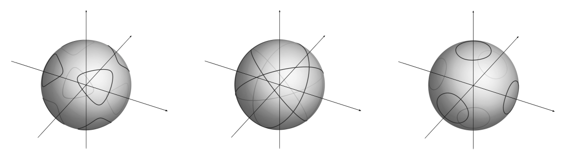
We can see that are invariant under permuting coordinates and coordinate reflections, i.e. invariant under action of the full octahedral group. We shall call these transformations symmetries and consider set of points on with non-trivial stabilizer, called special points and denoted by in the sequel. The fundamental domain is given by and the representatives of special points are the boundary points. On this boundary, there are exactly two (representative) paths connecting the points and , namely
Note that . We will also consider special points on for , namely
The characterization of these special points is gathered in the following elementary lemma.
Lemma 9.
Let be the set defined in (1) with , and let denote the (sub)sets of special points on , as defined above. Then
-
(a)
is not a special point if and only if are non-zero and pairwise distinct.
-
(b)
for we have , up to symmetries,
-
(c)
for we have , up to symmetries,
-
(d)
for the set contains, up to symmetries, exactly one point in and one point in . The representatives of special points are:
In particular, and .
Proof.
Point (a) follows immediately from the fact that points with a zero coordinate are exactly the points invariant under certain coordinate reflection and the points with two equal coordinates are points invariant under certain permutation.
Points (b) and (c) follow from the equality conditions in (2).
For (d) let us consider the system of equations, corresponding to special points with two equal coordinates,
Here is always the solution with non-negative coordinates satisfying for all , which leads to the point . The second solution has real positive coordinates only if and in this case , which leads to the point in this range of . The second type of special points are the points of the form with , which corresponds to the system of equations
The solution exists only for and is equal to , which leads to for . ∎
One can easily verify that defines a differentiable manifold for . Nevertheless, we will prove this fact along the way at the end of Section 4.2.
4.2. New system of variables
In this section we fix . Let us introduce the following change of variables,
The map is a diffeomorphism between and the hyperplane
with an inverse
which yields bijections of sets,
Notice that the symmetries in correspond to automorphisms of , which will be called induced symmetries. Since the symmetries can be represented as generalized permutation matrices with entries, by checking the image of a symmetry under , we can see that the induced symmetries are compositions of negation of a vector and permutations of its coordinates in (restricted to ). By induced special points we define the points on with non-trival stabilizer under action of the induced symmetries. Clearly is precisely the set of induced special points on .
Now, since for any and , we have
considering the constraints on composed with the map on yields
Therefore, for , where
| (3) |
Notice that is open in (since the set of induced special points is clearly closed), and
| (4) |
is of full rank for any , by the following lemma.
Lemma 10.
Suppose that is not an induced special point. Then,
-
(a)
the set contains at least 7 distinct elements.
-
(b)
the matrix defined in (4) has rank three.
Proof.
(a) It suffices to show that are pairwise distinct. If, say, , then and if then and thus in both cases .
(b) If , then we can assume , since other cases are similar. Consequently,
This matrix has rank three as are pairwise distinct by (a). To see this compute the determinant of matrix obtained by deleting the last column.
For , note that dividing a row or column by a non-zero number does not change the rank. Thus,
Note that any submatrix of the last matrix is of Vandermonde type, and thus has rank three as are distinct by (a). ∎
Therefore, is a differentiable manifold, and since is a diffeomorphism with , this implies that is in fact a differentiable manifold diffeomorphic to .
4.3. The function and its properties
Let us introduce the following lemmas needed in the proof of Lemma 8.
Lemma 11.
Suppose that is an even function with strictly convex fourth derivative. Then for every , the equation
| (5) |
has at most three real solutions.
Proof.
Since both and are odd functions, it is enough to prove that there is at most one positive solution. Notice that for , equation (5) is equivalent to
and it suffices to prove the monotonicity of the left side. Since is even and strictly convex, it follows that is strictly increasing on . Thus, is (strictly) convex on , which implies the monotonicity of slopes for . Therefore, both and are strictly increasing on , which ends our proof. ∎
Lemma 12.
Suppose that is an even function with strictly convex fourth derivative. For any , function
is strictly increasing.
Proof.
Define for , and notice that
thus, it is enough to prove the monotonicity of on . Equivalently, for , and it suffices to show that is strictly increasing on . Since , we need for . Notice that and for some by the mean value theorem, and since is strictly increasing on as an even strictly convex function, we have on . Thus, on , which ends the proof. ∎
4.4. Proof of Lemma 8
We now have enough tools to prove Lemma 8. In the following section we will consistently use the formulation of Lemma 8 along with notations from Sections 4.1, 4.2.
Proof of Lemma 8.
Throughout the proof we will assume and , since otherwise, the claims (a) and (b) follow instantly.
We will begin with the claim (a), i.e. the existence and uniqueness of . The set is non-empty if and only if . Let us consider the system of equations
When this system has a unique solution satisfying , namely
which leads to the point . For the solution satisfying exists if and only if and is given by
This proves the existence and uniqueness of , provided that . For one has when , whereas and for , which gives existence and uniqueness of .
Let us move on to the proof of (b). Firstly, we prove the claim for all even functions with strictly convex fourth derivative. The proof is by induction, and the main part concerns the base case.
Suppose that . Notice that we can fix since is an even function with strictly convex fourth derivative. Then with by the non-emptiness of , and the cases follow directly from Lemma 9(b,c). Therefore we assume , and consider
This is a function on , and a diffeomorphism yields a bijection of sets
We will prove that these sets are empty. Suppose otherwise, and notice that given by
is a function on , satisfying on . Therefore, using Lagrange multipliers theorem for on (which can be used due to the definition of in (3) and Lemma 10(b)), any critical point of on satisfies the system of equations
for some . Multiplying equations respectively by , implies that
| (6) |
where , and . Define
and note that by Vieta’s formulas
where . Since , we have , consequently by Lemma 9(a). Thus,
for some , and any solution of (6) yields
Since both sides are even functions of , the last equation is satisfied for any , thus has at least 7 distinct solutions by Lemma 10(a). Therefore, by Rolle’s theorem, equation
has at least four distinct solutions, which is in contradiction with Lemma 11.
Therefore, there are no critical points of on , and by compactness of the function attains extremal values in . By Lemma 9(d) in there are, up to symmetries, exactly two points, and . Since is invariant under symmetries, it is enough to prove that
which would imply that the maximal and minimal values are attained only in and , respectively. Note that we cannot have an equality for any , since this would imply that is constant on , and every point on would be critical. Moreover, using continuity of together with the intermediate value property, it is enough to check the inequality for a single . Taking , and using formulas for from Lemma 9(d), we can see that
is equivalent to , which holds due to the Lemma 12 for , .
We now move on to the inductive step. Fix and suppose that the claim (b) holds for all even with strictly convex . We will prove that the same is true for . By compactness of in the function attains maximal and minimal value at some and , respectively. Assuming, and , it is enough to prove that and . For fixed consider
The functions are even with strictly convex fourth derivative, so applying induction hypothesis to on for and gives by the form of maximizers in dimension . Thus, by uniqueness of , we obtain . Similarly, yield , ending this part.
To conclude the proof for all even functions with convex fourth derivative, notice that every such function is a pointwise limit of a sequence of even functions with strictly convex fourth derivative, for which we know that the extrema of the corresponding functions are attained at . Since these functions converge pointwise as well, passing to the limit for any fixed yields the claim. ∎
5. Proof of Proposition 3
We shall use the following lemma.
Lemma 13.
For any positive integer and we have
Proof.
Recall that and let for . Then, . Let be the number of such that . Notice that (we set ) and the sequence is non-decreasing for , thus
By Corollary 1 of [1] we have
Thus,
∎
We are now ready to prove the proposition.
References
- [1] Ahle, T.D., Sharp and simple bounds for the raw moments of the binomial and Poisson distributions, Statistics & Probability Letters 182, 2022, 109306.
- [2] Czerwiński, W., Khinchine inequalities (in Polish), University of Warsaw, Master Thesis, 2008.
- [3] Haagerup, U., The best constants in the Khintchine inequality. Studia Math. 70 (1981), no. 3, 231–283.
- [4] Havrilla, A., Nayar, P., Tkocz, T., Khinchin-type inequalities via Hadamard’s factorisation, Int. Math. Res. Not. 2023 (3), 2023, 2429–-2445.
- [5] Jakimiuk, J, Stability of Khintchine inequalities with optimal constants between the second and the -th moment for , 2025, arXiv:2503.07001
- [6] Khintchine, A., Über dyadische Brüche. Math. Z. 18 (1923), no. 1, 109–116.
- [7] Littlewood, J. E., On a certain bilinear form, Quart. J. Math., Oxford Ser. 1 (1930), 164–174.
- [8] Mordhorst, O., The optimal constants in Khintchine’s inequality for the case , Colloquium Mathematicum 147, 2017, 203–216.
- [9] Nayar P., Oleszkiewicz K., Khinchine type inequalities with optimal constants via ultra log-concavity, Positivity, 16 (2012), 359–371.
- [10] Nazarov, F. L., Podkorytov, A. N., Ball, Haagerup, and distribution functions, Complex analysis, operators, and related topics, Oper. Theory Adv. Appl., 113 (2000), 247–267,
- [11] Szarek, S. J., On the best constants in the Khinchin inequality, Studia Math. 58 (1976), no. 2, 197–208.
- [12] Whittle, P., Bounds for the moments of linear and quadratic forms in independent random variables, Theory Probab. Appl. 5 (1960), 302–305.
- [13] Young, R.M.G., On the best possible constants in the Khintchine inequality, J. London Math. Soc. 14 (2), 1976, 496–504.