Corrected Riemann smoothed particle hydrodynamics method for multi-resolution fluid-structure interaction

Abstract

As a mesh-free method, smoothed particle hydrodynamics (SPH) has been widely used for modeling and simulating fluid-structure interaction (FSI) problems. While the kernel gradient correction (KGC) method is commonly applied in structural domains to enhance numerical consistency, high-order consistency corrections that preserve conservation remain underutilized in fluid domains despite their critical role in FSI analysis, especially for the multi-resolution scheme where fluid domains generally have a low resolution. In this study, we incorporate the reverse kernel gradient correction (RKGC) formulation, a conservative high-order consistency approximation, into the fluid discretization for solving FSI problems. RKGC has been proven to achieve exact second-order convergence with relaxed particles and improve numerical accuracy while particularly enhancing energy conservation in free-surface flow simulations. By integrating this correction into the Riemann SPH method to solve different typical FSI problems with a multi-resolution scheme, numerical results consistently show improvements in accuracy and convergence compared to uncorrected fluid discretization. Despite these advances, further refinement of correction techniques for solid domains and fluid-structure interfaces remains significant for enhancing the overall accuracy of SPH-based FSI modeling and simulation.

1 Introduction

Fluid-structure interaction (FSI), a classical multiphysics problem characterized by the bidirectional coupling between fluids and deformable structures, is ubiquitous in nature, as seen in fish swimming, jellyfish pulsation, and insect flight, and critical to engineering applications such as wave-ship impacts, aircraft wing flutter, and blood-arterial wall dynamics. Understanding FSI is fundamental to designing and optimizing these systems. However, the inherent nonlinearity, time-dependent behavior, and moving fluid-structure interfaces pose significant numerical challenges, particularly when large deformations and free surfaces are involved [1, 2, 3].

Grid-based methods like the finite element method (FEM) [4] have dominated numerical computations and are widely applied for solving FSI problems. Techniques such as the immersed boundary method (IBM) [5], volume of fluid (VOF) [6], and level set methods [7] are often employed to track moving interfaces and free surfaces. Despite their widespread use, these methods face challenges in capturing sharp interfaces, ensuring mass conservation, and managing computational costs during frequent mesh updates for large structural deformations.

Lagrangian mesh-free methods, including smoothed particle hydrodynamics (SPH) [8, 9], the discrete element method (DEM) [10], and the moving particle semi-implicit method (MPS) [11], offer advantages for FSI problems due to their advantages in handling free surfaces, large deformations, and material interfaces. Hybrid approaches like SPH-FEM [12, 13, 14, 15] and MPS-FEM [16, 17] combine Lagrangian particle methods for fluid modeling with FEM for structural analysis. While these methods improve numerical results, they still require careful treatment of fluid-structure interface boundary conditions. Fully Lagrangian particle methods, such as SPH-SPH [18, 19, 20, 21, 22, 23], ISPH-SPH [24, 25], and MPS-MPS [26, 27], provide consistent modeling for both fluid and solid domains but numerical accuracy and stability remain key challenges for these Lagrangian particle methods.

To improve SPH consistency, methods like kernel gradient correction (KGC) [28], reproducing kernel particle methods (RKPM) [29, 30], and corrective smoothed particle methods (CSPM) [31], the finite particle method [32], modified SPH (MSPH) [33, 34, 35, 36], moving least squares (MLS) [37], and other high-order methods [38, 39, 40] have been proposed. These techniques enhance the accuracy of gradient and Laplacian operator approximations. KGC, in particular, has been widely used for modeling solid structures [41, 20, 22] within the total Lagrangian framework, where it is used for discreting both momentum equations and deformation gradient tensors, demonstrating robustness in large-deformation analyses. For fluid simulations, various KGC-liked corrections have been introduced to improve consistency while preserving conservation, such as averaged correction matrices [42, 43, 44] and pairwise particle corrections [45, 46], etc. However, these approaches fail to achieve true high-order consistency [47].

Despite these attempts and advancements, key challenges remain. One significant difficulty is the trade-off between high-order consistency and momentum conservation [47]. While momentum conservation is important for numerical accuracy, most existing KGC implementations only rely on non-conservative formulations, limiting their applicability to systems governed by strict conservation laws. Another challenge arises in the correction implementation of free-surface flows involving violent phenomena such as dam breaks [48] and sloshing flows [25], where rapid fluid fragmentation and extreme interface deformations can lead to ill-conditioned correction matrices, numerical errors, and simulation instabilities. Accurate fluid predictions are essential in FSI modeling since fluid dynamics errors propagate directly to the fluid-structure coupling, particularly in multi-resolution schemes where the fluid generally has a low resolution. Improving fluid accuracy enhances overall fidelity and ensures reliable predictions of complex interactions, such as force transmission and structural response.

In this study, we integrate the reverse kernel gradient correction (RKGC) method into the fluid domain discretization when solving FSI problems. RKGC has been shown to satisfy first-order consistency in conservative formulations when proper particle relaxation is achieved and demonstrates improved accuracy in fluid simulations and fluid-rigid interactions [47]. Building on this framework, both fluid and elastic solid domains are solved using the Riemann SPH method, where Riemann solutions govern particle-pair interactions. To ensure high-order consistency, non-dissipative terms in the fluid discretization are replaced with the RKGC formulation. The correction matrix for the fluid flow is updated at each advection time step, with additional weighted treatments for free-surface regions to maintain numerical stability. A multi-resolution scheme with larger fluid particle spacing balances accuracy and computational efficiency. Numerical results consistently demonstrate that the proposed RKGC-corrected Riemann SPH method significantly improves accuracy in FSI simulations of both internal and free surface flows.

The remainder of this paper is organized as follows. Section 2 presents the SPH discretization for fluid, structure, and fluid-structure interactions, along with details of the RKGC Riemann SPH method. Section 3 validates the method through extensive numerical examples. Section 4 summarizes the key findings and suggests future research directions.

2 Numerical method

2.1 Fluid model

The governing equations for an isothermal Newtonian fluid in the updated Lagrangian framework are the mass and momentum conservation equations, expressed as

$$\begin{cases}\vskip 5.0pt\displaystyle\dfrac{\text{d}\rho}{\text{d}t}=-\rho\nabla\cdot\boldsymbol{\rm v}\\ \displaystyle\dfrac{\text{d}\boldsymbol{\rm v}}{\text{d}t}=-\dfrac{1}{\rho}\nabla p+\boldsymbol{\rm a}_{\rm v}+\boldsymbol{\rm g}+\boldsymbol{\rm a}^{S:F},\end{cases}$$ (1)

where $\rho$ is the fluid density, $t$ the time, $\boldsymbol{\rm v}$ the velocity, and $p$ the pressure. The term $\boldsymbol{\rm a}_{\rm v}=\nu\nabla^{2}\boldsymbol{\rm v}$ represents the viscous acceleration with $\nu$ the kinematic viscosity, $\boldsymbol{\rm g}$ the gravitational acceleration, and $\boldsymbol{\rm a}^{S:F}=\boldsymbol{\rm f}^{S:F}/m$ denotes the interaction acceleration acting on the fluid due to the solid structure, where $\boldsymbol{\rm f}^{S:F}$ comprises both viscous and pressure forces and $m$ is the mass of the particle. In addition, $\text{d}(\bullet)/\text{d}t=\partial(\bullet)/\partial t+\boldsymbol{\rm v}\cdot\nabla(\bullet)$ refers to the material derivative. To close the governing equations, an artificial equation of state (EoS) for weakly compressible flows is applied:

$$p={c_{0}}^{2}\left(\rho-\rho_{0}\right).$$ (2)

Here, $\rho_{0}$ is the initial density, and $c_{0}$ denotes the artificial sound speed. Setting $c_{0}=10U_{\rm max}$, where $U_{\rm max}$ represents the anticipated maximum fluid speed, satisfies the weakly compressible assumption where the density variation remains around 1% [49].

The Riemann-SPH method [50], which predicts inter-particle interactions via the Riemann solver, is employed to mitigate pressure oscillations in weakly compressible SPH (WCSPH). Additionally, a multi-resolution SPH method is adopted to enhance computational efficiency [22, 25, 13, 51]. Subsequently, the continuity and momentum equations are discretized as

$$\begin{cases}\vskip 5.0pt\displaystyle\dfrac{\text{d}\rho_{i}}{\text{d}t}=2\rho_{i}\sum_{j}\left(\boldsymbol{\rm v}_{i}-\boldsymbol{\rm v^{*}}\right)\cdot\nabla W_{ij}^{h^{F}}V_{j}\\ \displaystyle\dfrac{\text{d}\boldsymbol{\rm v}_{i}}{\text{d}t}=-\dfrac{2}{m_{i}}\sum_{j}P^{*}\nabla W_{ij}^{h^{F}}V_{i}V_{j}+2\sum_{j}\dfrac{\nu}{\rho_{i}}\frac{\boldsymbol{\rm v}_{ij}}{r_{ij}}\dfrac{\partial W_{ij}^{h^{F}}}{\partial{r_{ij}}}V_{j}+\boldsymbol{\rm g}_{i}+\boldsymbol{\rm a}_{i}^{S:F}\left(h^{F}\right),\end{cases}$$ (3)

where $V_{i}$ is the particle volume, $\nabla W_{ij}^{h^{F}}=\nabla W\left(\boldsymbol{\rm r}_{ij},h^{F}\right)=\frac{\boldsymbol{\rm e}_{ij}}{r_{ij}}\frac{\partial W_{ij}}{\partial r_{ij}}$, where $\boldsymbol{\rm r}_{ij}=\boldsymbol{\rm r}_{i}-\boldsymbol{\rm r}_{j}$ and $h^{F}$ is the smoothing length of the fluid, the unit vector $\boldsymbol{\rm e}_{ij}=\frac{\boldsymbol{\rm r}_{ij}}{r_{ij}}$, denoting the derivative of the kernel function with respect to $\boldsymbol{\rm{r}}_{i}$, the position of the particle $i$. The particle-pair velocity $\boldsymbol{\rm v}^{*}$ and pressure $P^{*}$ are solutions obtained from the Riemann problem constructed along the interacting line of each pair of particles [50, 52], where the left and right states of the Riemann problem are defined as

$$\begin{cases}\left(\rho_{L},U_{L},P_{L}\right)=\left(\rho_{i},\boldsymbol{\rm v}_{i}\cdot\boldsymbol{\rm e}_{ij},p_{i}\right)\\ \left(\rho_{R},U_{R},P_{R}\right)=\left(\rho_{j},\boldsymbol{\rm v}_{j}\cdot\boldsymbol{\rm e}_{ij},p_{j}\right).\end{cases}$$ (4)

Using a linearized Riemann solver, the solutions for intermediate velocity and pressure are given by

$$\begin{cases}\vskip 5.0pt\boldsymbol{\rm v}^{*}=\overline{\boldsymbol{\rm v}}_{ij}+\left(U^{*}-\overline{U}_{ij}\right)\boldsymbol{\rm e}_{ij}\quad\\ U^{*}=\overline{U}_{ij}+\dfrac{1}{2}\dfrac{(p_{i}-p_{j})}{\rho_{0}c_{0}}\\ P^{*}=\overline{p}_{ij}+\dfrac{1}{2}\beta\rho_{0}c_{0}U_{ij}.\end{cases}$$ (5)

Here, $\overline{(\bullet)}_{ij}=\left[(\bullet)_{i}+(\bullet)_{j}\right]/2$ denotes the particle-pair average, $\overline{U}_{ij}=-\overline{\boldsymbol{\rm v}}_{ij}\cdot\boldsymbol{\rm e}_{ij}$ and $U_{ij}=-\boldsymbol{\rm v}_{ij}\cdot\boldsymbol{\rm e}_{ij}$, represents the particle-pair average and difference of the particle velocity along the interaction line, respectively. The low-dissipation limiter, defined as $\beta=\min\left(3\max\left(U_{ij}/c_{0},0\right),1\right)$, is introduced to reduce the inherent numerical dissipation and enhance the discretization accuracy.

2.2 Structure model

The solid structure is considered an elastic and weakly compressible material. The governing equations in the total Lagrangian framework read as

$$\begin{cases}\vskip 5.0pt\displaystyle\rho^{S}=\left(\rho^{S}\right)^{0}J^{-1}\\ \left(\displaystyle\dfrac{\text{d}\boldsymbol{\rm v}}{\text{d}t}\right)^{S}=\dfrac{1}{\rho^{0}}\nabla^{0}\cdot\mathbb{P}^{T}+\boldsymbol{\rm g}+\boldsymbol{\rm a}^{F:S},\end{cases}$$ (6)

where $\rho^{S}$ is the solid density, $\left(\rho^{S}\right)^{0}$ is the initial reference density, and $J={\rm det}\left(\mathbb{F}\right)$ denotes the Jacobian determinant of the deformation gradient tensor $\mathbb{F}$. The operator $\nabla^{0}\left(\bullet\right)\equiv\partial\left(\bullet\right)/\partial\boldsymbol{\rm r}^{0}$ represents the gradient with respect to the initial reference configuration. The superscript $\left(\bullet\right)^{0}$ indicates quantities in the initial reference state. $\mathbb{P}^{T}$ is the nominal stress tensor, which is the transpose of the first Piola–Kirchhoff stress tensor $\mathbb{P}$. Additionally, $\boldsymbol{\rm a}^{F:S}$ represents the acceleration induced by fluid-structure interaction.

For a Kirchhoff material, the first Piola–Kirchhoff stress tensor is given by

$$\mathbb{P}=\mathbb{F}\mathbb{S},$$ (7)

where the deformation gradient tensor $\mathbb{F}$ reads

$$\mathbb{F}=\nabla^{0}\boldsymbol{\rm u}+\mathbb{I},$$ (8)

with $\boldsymbol{\rm u}=\boldsymbol{\rm r}-\boldsymbol{\rm r}^{0}$ representing the displacement and $\mathbb{I}$ the identity matrix. The second Piola–Kirchhoff stress tensor $\mathbb{S}$ is related to the Green–Lagrange strain tensor $\mathbb{E}$ by the constitutive relation

$$\mathbb{E}=\dfrac{1}{2}\left(\mathbb{F}^{T}\mathbb{F}-\mathbb{I}\right).$$ (9)

For a linear elastic and isotropic material, the constitutive equation reads

$$\displaystyle\mathbb{S} =K{\rm tr}\left(\mathbb{E}\right)\mathbb{I}+2G\left(\mathbb{E}-\dfrac{1}{3}{\rm tr}\left(\mathbb{E}\right)\mathbb{I}\right)$$

$$=\lambda{\rm tr}\left(\mathbb{E}\right)\mathbb{I}+2\mu\mathbb{E},$$ (10)

where $\lambda$ and $\mu$ are the Lamé parameters [53]. The bulk modulus is given by $K=\lambda+\left(2\mu/3\right)$, and the shear modulus is $G=\mu$. These parameters are related to the Young’s modulus $E$ and the Poisson ratio $\nu$ through

$$E=2G\left(1+2\nu\right)=3K\left(1-2\nu\right).$$ (11)

For weakly compressible materials, the speed of sound in the solid structure is defined as $c^{S}=\sqrt{K/\rho^{S}}$.

The discretization of the governing equations in Eq. (6) at particle $a$ is expressed as

$$\begin{cases}\vskip 5.0pt\displaystyle\left(\rho^{S}\right)_{a}=\left(\rho^{S}\right)^{0}_{a}{\rm det}\left(\mathbb{F}_{a}\right)^{-1}\\ \displaystyle\left(\dfrac{\rm d\boldsymbol{{\rm v}}}{\rm dt}\right)^{S}_{a}=\dfrac{1}{m_{a}}\sum_{b}\left(\mathbb{P}_{a}\mathbf{B}^{0}_{a}+\mathbb{P}_{b}\mathbf{B}^{0}_{b}\right)\nabla^{0}W^{h^{S}}_{ab}V_{a}V_{b}+\boldsymbol{\rm g}_{a}+\boldsymbol{\rm a}_{a}^{F:S}\left(h^{S}\right),\end{cases}$$ (12)

with the deformation gradient tensor discretized as

$$\mathbb{F}_{a}=\left(\sum_{b}\left(\boldsymbol{\rm u}_{b}-\boldsymbol{\rm u}_{a}\right)\otimes\nabla^{0}W_{ab}^{h^{S}}V_{b}\right)\mathbf{B}^{0}_{a}+\mathbb{I},$$ (13)

where $h^{S}$ is the smoothing length for the solid structure. The correction matrix $\mathbf{B}$ [28, 41], which mitigates kernel inconsistency, is computed in the initial reference configuration as

$$\mathbf{B}^{0}_{a}=\left(\sum_{b}\left(\boldsymbol{\rm r}^{0}_{b}-\boldsymbol{\rm r}^{0}_{a}\right)\otimes\nabla^{0}W^{h^{S}}_{ab}V_{b}^{0}\right)^{-1}.$$ (14)

2.3 Fluid–structure coupling

In fluid-structure interaction, structure particles are treated as a moving boundary for fluid particles, providing necessary boundary conditions for solving the momentum and continuity equations. To ensure proper interaction, the smoothing length $h^{F}$ is chosen such that $h^{F}\geq h^{S}$, allowing a solid particle $a$ to be recognized and tagged as a neighbor of a fluid particle $i$. The interaction acceleration exerted by the structure on the fluid is given by

$$\boldsymbol{a}_{i}^{S:F}=-\dfrac{2}{m_{i}}\sum_{a}P^{*}\nabla W^{h^{F}}_{ia}V_{i}V_{a}+2\sum_{a}\dfrac{\nu}{\rho_{i}}\dfrac{\boldsymbol{\rm v}_{i}-\boldsymbol{\rm v}_{a}^{d}}{r_{ia}}\dfrac{\partial W_{ia}^{h^{F}}}{\partial r_{ia}}V_{a},$$ (15)

where the first and second terms on the right-hand side represent the accelerations induced by fluid pressure and viscous forces, respectively. Here, $i$ refers to a fluid particle, and $a$ denotes a structure particle. The pressure term $P^{*}$ is obtained from a one-sided Riemann-based scheme [51], where the left and right states are defined as

$$\begin{cases}\left(\rho_{L},U_{L},P_{L}\right)=\left(\rho_{i},-\boldsymbol{\rm v}_{i}\cdot\boldsymbol{\rm n}_{a},p_{i}\right)\\ \left(\rho_{R},U_{R},P_{R}\right)=\left(\rho_{a},-\boldsymbol{\rm v}_{a}^{d}\cdot\boldsymbol{\rm n}_{a},p_{a}^{d}\right),\end{cases}$$ (16)

where $\boldsymbol{\rm n}_{a}$ is the local normal vector pointing from the solid to the fluid. The imaginary pressure $p^{d}{a}$ and velocity $\boldsymbol{\rm v}_{a}^{d}$ are derived based on the no-slip boundary condition at the fluid–structure interface as

$$\begin{cases}\vskip 5.0pt\displaystyle p^{d}_{a}=p_{i}+\rho_{i}{\rm max}\left(0,\left(\boldsymbol{\rm g}-\frac{\widetilde{\rm d\boldsymbol{\rm v}_{a}}}{\rm dt}\right)\right)\cdot\boldsymbol{\rm r}_{ia}\\ \boldsymbol{\rm v}_{a}^{d}=2\boldsymbol{\rm v}_{i}-\boldsymbol{\rm\widetilde{v}}_{a}.\end{cases}$$ (17)

Here, $\frac{\widetilde{\rm d\boldsymbol{\rm v}_{a}}}{\rm dt}$ and $\boldsymbol{\rm\widetilde{v}}_{a}$ represent the time-averaged acceleration and velocity of solid particles over one fluid acoustic time step [54] to resolve the mismatch between force and acceleration when using the multi-resolution scheme [22, 51]. Consequently, the interaction acceleration $\boldsymbol{a}_{i}^{F:S}$ exerted by the fluid on the solid structure can be determined in a straightforward manner.

2.4 RKGC Riemann SPH and transport velocity formulation

For a smooth field $\psi\left(\boldsymbol{\rm r}\right)$, the SPH approximation of its gradient using the reverse kernel gradient correction (RKGC) [47] at a particle position $\boldsymbol{\rm r}_{i}$ can be expressed as

$$\nabla\psi_{i}=-\sum_{j}\left(\psi_{i}\mathbf{B}_{j}+\psi_{j}\mathbf{B}_{i}\right)\nabla W_{ij}V_{j},$$ (18)

where the KGC matrix is applied in reverse order with respect to particles $i$ and $j$, and $\mathbf{B}_{i}$ is the correction matrix [28], defined as

$$\mathbf{B}_{i}=\left(-\sum_{j}\mathbf{r}_{ij}\otimes\nabla W_{ij}V_{j}\right)^{-1}.$$ (19)

The calculation in Eq. (19) follows the same formulation as in Eq. (6), except that the current version for fluids is based on the updated configuration and calculated in each advection time step [54]. The gradient approximation in Eq. (18) has been shown to exactly satisfy first-order consistency when particle relaxations are based on $\mathbf{B}_{i}$ and $\mathbf{B}_{j}$, a form of “geometric stress” that depends on particle positions. Accordingly, the original particle-pair average term in the Riemann solution, given in Eq. (5) as $\overline{(\bullet)}_{ij}=\left[(\bullet)_{i}+(\bullet)_{j}\right]/2$, is modified in the momentum equation as

$$\overline{p}_{ij}\Rightarrow\overline{\left(p\mathbf{B}\right)}_{ij}=\frac{1}{2}\left(p_{i}\mathbf{B}_{j}+p_{j}\mathbf{B}_{i}\right),$$ (20)

to improve pressure prediction accuracy in solving fluid-structure interaction (FSI) problems. A previous study [47] demonstrated that applying the kernel gradient correction (KGC) in the continuity equation has negligible impact on simulation results for the Lagrangian SPH method. Following this observation, we adopt the same practice in the present study without correction on the continuity equation.

However, computing the correction matrix may lead to numerical instability, particularly in simulations of violent free-surface flows [43]. For example, during wave breaking and splashing events, the correction matrix can become ill-conditioned, introducing significant errors and instability. To address this issue, the weighted kernel gradient correction (WKGC) [55] is employed, where the KGC matrix near the free surface region is weighted with the identity matrix (WKGC¹) to improve numerical robustness. In this approach, the weighted KGC matrix is defined as

$$\widetilde{\mathbf{B}}_{i}=\omega_{1}\mathbf{B}_{i}+\omega_{2}\mathbf{I},$$ (21)

where the weighting coefficients $\omega_{1}$ and $\omega_{2}$ are given by

$$\begin{cases}\vskip 5.0pt\displaystyle\omega_{1}=\frac{\left|\mathbf{A}_{i}\right|}{\left|\mathbf{A}_{i}\right|+\kappa_{i}}\\ \displaystyle\omega_{2}=\frac{\kappa_{i}}{\left|\mathbf{A}_{i}\right|+\kappa_{i}}.\end{cases}$$ (22)

Here, $\left|\mathbf{A}_{i}\right|=\left|\mathbf{B}_{i}^{-1}\right|$ serves as a smoothness indicator for the correction matrix, while $\kappa_{i}=\max\left(\alpha-\left|\mathbf{A}_{i}\right|,0\right)$ determines the weighting applied to the identity matrix. The parameter $\alpha$ acts as a threshold to regulate the weighting process. Further details on this approach can be found in Ref. [55].

Since particle relaxation remains computationally expensive in Lagrangian SPH methods [56, 47]. To address this, a KGC-based transport velocity formulation is employed, which involves a single correction step per time step. The transport velocity $\widetilde{\boldsymbol{\rm v}}_{i}$ governs particle position updates via

$$\dfrac{\rm d\boldsymbol{\rm r}_{i}}{\rm{dt}}=\widetilde{\boldsymbol{\rm v}}_{i}.$$ (23)

Numerically, this formulation applies a one-step correction to particle positions during each advection time step [54],

$$\Delta\mathbf{r}_{i}=\eta\left(\Delta{x}\right)^{2}\sum_{j}(\mathbf{B}_{i}+\mathbf{B}_{j})\nabla W_{ij}V_{j},$$ (24)

where the parameter $\eta$ is generally chosen as 0.2 to ensures stability by aligning with the CFL number criteria in SPH [57]. Note that the transport velocity formulation is imposed on the internal flow but is not applied to free-surface flows due to the complexity of handling the free surface and general practices in SPH simulations [45, 55, 58, 47].

3 Numerical examples

In this section, we present several typical numerical cases to validate the enhanced accuracy of the proposed RKGC Riemann SPH method for modeling and simulating FSI problems. For all simulations, the C2 Wendland kernel is adopted with smoothing length $h^{F}=1.3dp^{F}$ and $h^{S}=1.15dp^{S}$, where $dp^{F}$ and $dp^{S}$ denote the initial particle spacing for the fluid and solid structure, respectively. In addition, according to the multi-resolution framework established in our prior work [22], a resolution ratio of $dp^{F}=2dp^{S}$ is employed unless otherwise stated, which strategically reduces the computational cost by coarsening the fluid particle resolution while preserving simulation accuracy through targeted refinement at fluid-structure interfaces.

3.1 Hydrostatic water column on an elastic plate

The first example presents a typical benchmark test involving a hydrostatic water column resting on an elastic aluminum plate, originally proposed by Fourey et al. [59]. This case has been widely adopted for FSI validation studies [22, 25, 60, 48, 61]. As illustrated in Fig. 1, the water tank has dimensions of 1.0 m (width) × 2.0 m (height).

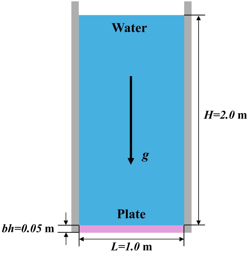
Figure 1: Hydrostatic water column on an elastic plate: Schematic illustration.

The tank’s bottom consists of an aluminum plate with a thickness of $bh=0.05$ m, a density of $\rho^{S}=2700~\mathrm{kg/m^{3}}$, a Young’s modulus of $E^{S}=67.5~\mathrm{GPa}$, and a Poisson’s ratio of $\nu^{S}=0.34$. At $t=0.0$ s, the plate is instantaneously subjected to the hydrostatic load. After initial oscillations, the FSI system reaches an equilibrium state. The theoretical equilibrium displacement at the plate’s mid-span, derived from the analytical model in Ref. [59], is $-6.85\times 10^{-5}$ m. Following established methodologies [59, 24, 22], a constant fluid time-step size of $\Delta t^{F}=2\times 10^{-5}$ s is employed, and the simulations terminate at $t=2.0$ s. The artificial damping method from Ref. [62] is also adopted to mitigate the oscillations.

Fig. 2 shows fluid pressure and structural von Mises stress distributions at $t=0.5$ s for the RKGC method at the resolution $bh/dp^{S}=8$.

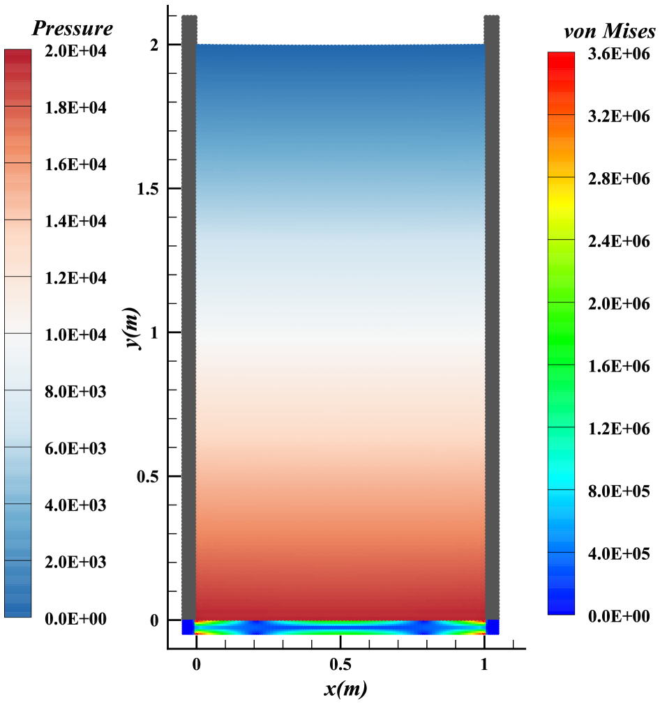
Figure 2: Hydrostatic water column on an elastic plate: Distributions of fluid pressure and structural von Mises stress fields at $t=0.5~\mathrm{s}$.

The present RKGC corrected method predicts smooth pressure and stress fields in the respective domains, aligning with the results reported in Refs. [63, 25], indicating good numerical stability. The time history of the vertical mid-span displacement of the elastic plate predicted by different methods, as well as for different resolutions of the present method, is presented in Fig. 3.

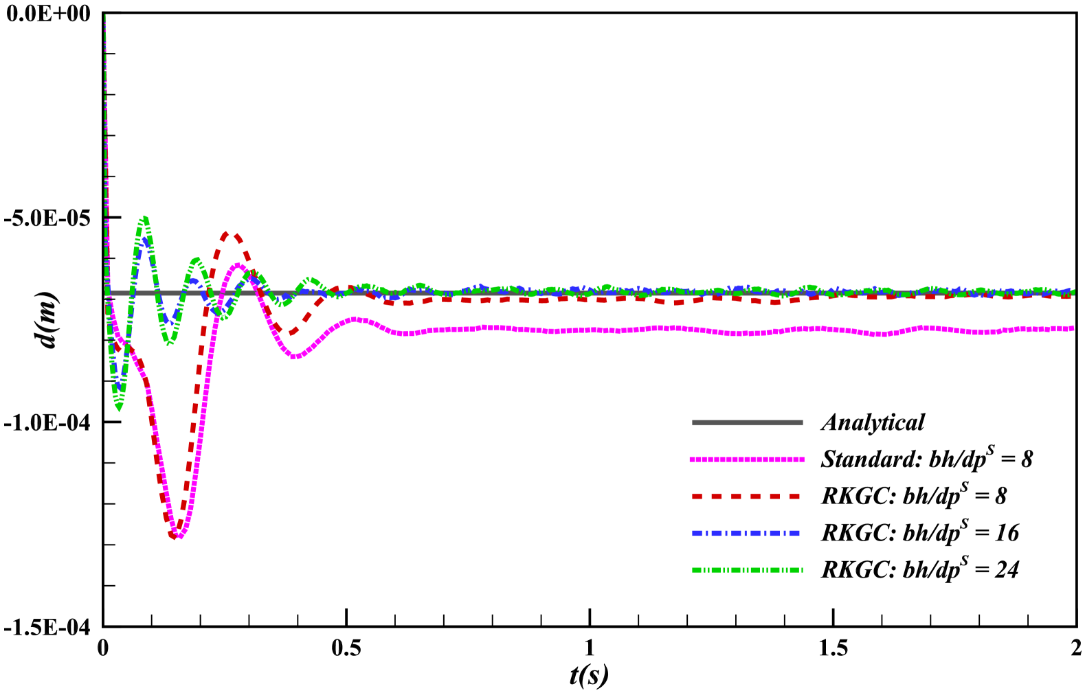
Figure 3: Hydrostatic water column on an elastic plate: Time history of the vertical mid-span displacement of the elastic plate.

The standard SPH method predicts a displacement of $-8.0\times 10^{-5}$ m at the resolution $bh/dp^{S}=8$, consistent with the findings of Zhang et al. [22] (as shown in their Fig. 3(b)) and Khayyer et al. [24, 25] (as shown in their Fig. 8 at $bh/dp^{S}=12$ and Fig. 6 at $bh/dp^{S}=10$, respectively). In contrast, the RKGC SPH method predicts a displacement at the same resolution that closely aligns with the analytical solution from Ref. [59]. This is because the pressure force from the water primarily drives the displacement of the aluminum plate, and the RKGC method improves the accuracy of the pressure predictions. With the resolution increases, the results converge toward the analytical solution, demonstrating the good convergence of the proposed method.

To validate the energy conservation property of the present method, Fig. 4 illustrates the time history of the normalized total energy of the system computed using different methods, as well as for different resolutions of the present method.

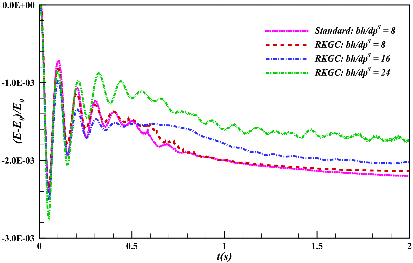
Figure 4: Hydrostatic water column on an elastic plate: Time history of the normalized total energy for different methods.

The total energy drops at a rate between $-2.0\times 10^{-3}$ and $-1.0\times 10^{-3}$, which is consistent with the results reported in Refs. [22, 25]. The RKGC SPH method exhibits a slightly lower rate of energy decay compared to the standard SPH method at the lowest resolution, demonstrating the enhanced energy conservation property of the proposed method. As the resolution increases, the energy decay rate decreases, indicating the improved energy conservation.

3.2 Flow-induced vibration of a beam behind a cylinder

The second example involves two-dimensional flow-induced vibration (FIV) of a flexible beam attached to a rigid cylinder, corresponding to the widely studied FSI2 benchmark test proposed by Turek and Hron [64]. The computational setup, illustrated in Fig. 5, features a rigid cylinder of diameter $D=1$ centered at $(2D,2D)$ within a domain spanning $11D\times 4.1D$. A sensor, labeled $M$, tracks the trajectory at the free end of the beam.

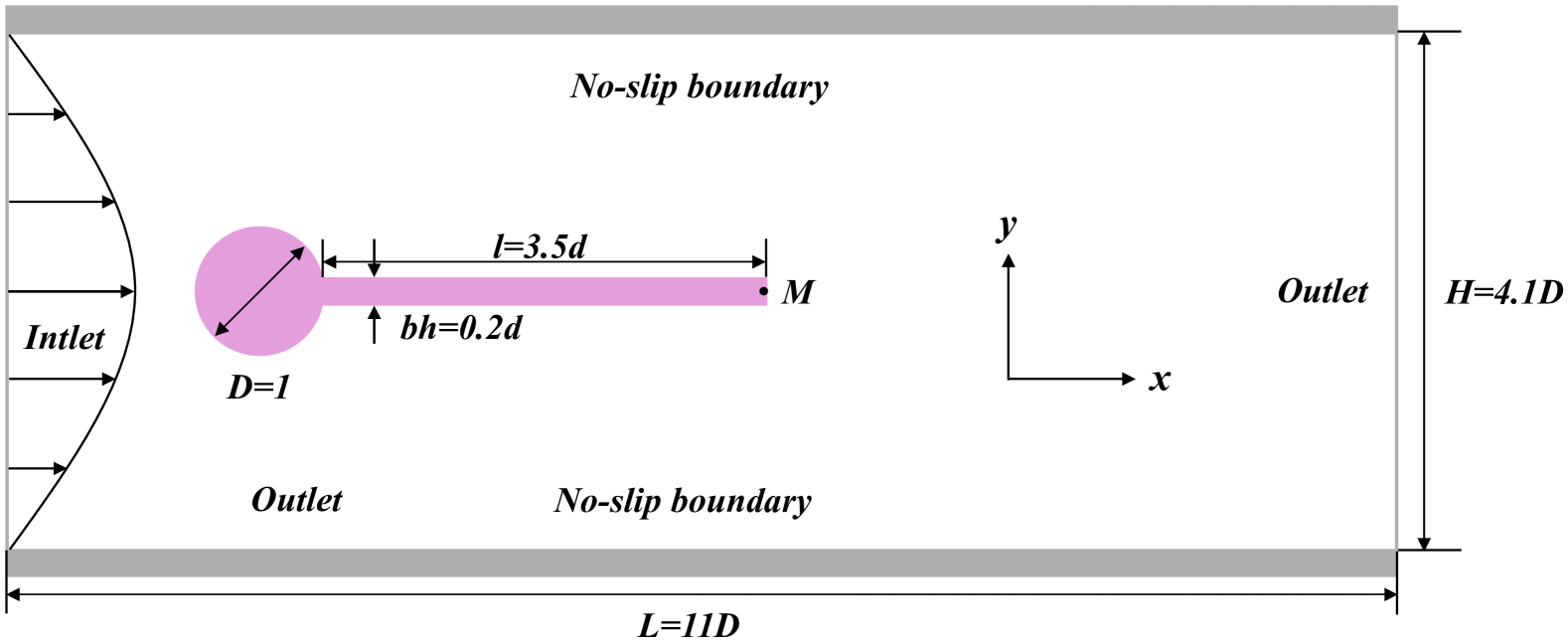
Figure 5: Flow-induced vibration of a beam behind a cylinder: Schematic illustrate. Sensor $M$ monitors the trajectory at the free end of the beam.

No-slip boundary conditions are enforced on the top and bottom walls, while the left and right boundaries are designated as inflow and outflow, respectively. The inflow velocity follows a time-dependent parabolic profile given by

$$U(y)=1.5\overline{U}(t,y)\frac{(H-y)y}{H^{2}},$$ (25)

where

$$\overline{U}(t,y)=\begin{cases}\vskip 5.0pt0.5U_{0}\left(1.0-\cos\left(0.5\pi t\right)\right)&\text{if }t<t_{s},\\ U_{0}&\text{otherwise},\end{cases}$$ (26)

with $U_{0}=1.0$ and $t_{s}=2.0$, and $H$ denoting the channel height. Consistent with previous studies [64, 20, 22, 65], the physical parameters replicate the challenging low-stiffness FSI2 benchmark test. The density ratio of the structure to the fluid is $\rho^{S}/\rho^{F}=10$, and the Reynolds number is $Re=\rho^{F}U_{0}D/\eta=100$. The beam is modeled as an isotropic linear elastic material with a dimensionless Young’s modulus $E^{*}=E^{S}/\rho^{F}/U^{2}_{0}=1.4\times 10^{3}$ and Poisson’s ratio $\nu^{S}=0.4$.

Fig. 6 shows the von Mises stress distribution in the elastic plate and the vorticity in the flow field at four time instants after self-sustained oscillations are established. These results, obtained using the present RKGC corrected method at the resolution $bh/dp^{s}=4$, demonstrate clear periodic motion consistent with other numerical results from Refs. [64, 66, 20, 22, 67].

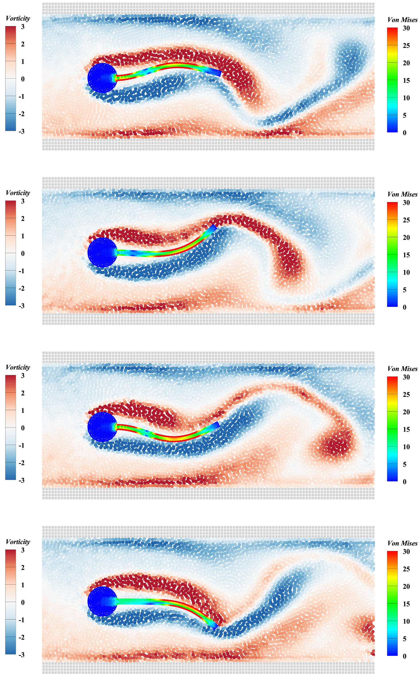
Figure 6: Flow-induced vibration of a beam behind a cylinder: Distributions of the von Mises stress in the elastic plate and the vorticity in the flow field at four time instants.

Fig. 7 presents the displacement amplitudes in the x-direction and y-direction, along with the trajectory of point $M$, obtained by different methods at the resolution $bh/dp^{s}=4$.

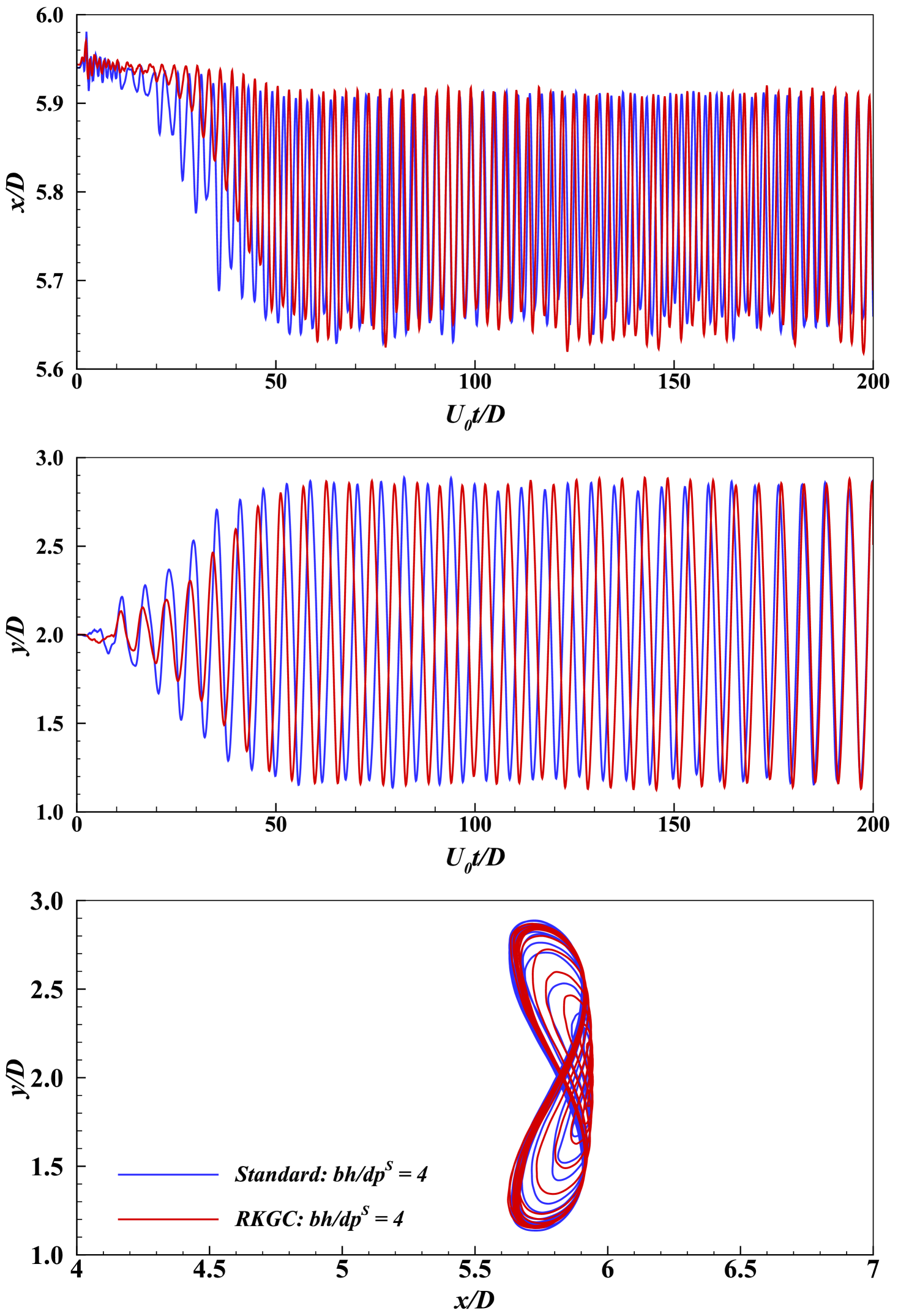
Figure 7: Flow-induced vibration of a beam behind a cylinder: Amplitude of the displacement in x-direction (top panel), amplitude of the displacement in y-direction (middle panel) and the trajectory (bottom panel) of point $M$ obtained by different methods.

As time exceeds a dimensionless value of 50, the beam exhibits periodic self-sustained oscillations. The trajectory of point $M$ follows a typical Lissajous curve, with a 2:1 frequency ratio between horizontal and vertical motions [64], indicating strong agreement with results reported in Refs. [64, 66, 22]. It is evident that at this resolution, the amplitudes obtained by the two methods are similar, while the frequency for the present RKGC method is clearly higher.

To enable a quantitative comparison, Table 1 presents reference results, results obtained using different methods, and convergence studies of the present RKGC method.

Table 1: Flow-induced vibration of a beam behind a cylinder: Comparison results with the reference and the convergence study of the present RKGC method.

Results source	Amplitude in y-axis	Frequency
Turek and Hron [64]	$0.830$	$0.190$
Bhardwaj and Mittal [66]	$0.920$	$0.190$
Tian et al. [68]	$0.784$	$0.190$
Han and Hu [20]	$0.886$	$0.168$
Zhang et al. [22]	$0.860$	$0.188$
Zheng et al. [67]	$1.090$	$0.174$
RKGC($bh/dp^{S}=12$)	$0.831$	$0.187$
RKGC($bh/dp^{S}=8$)	$0.833$	$0.183$
RKGC($bh/dp^{S}=4$)	$0.861$	$0.175$
Standard($bh/dp^{S}=4$)	$0.847$	$0.171$

At low resolution ($bh/dp^{S}=4$), the present method shows closer with reference amplitude and frequency values than the standard method, though both underestimate frequencies. Increasing resolution improves frequency predictions and reduces y-direction amplitude, converging toward literature values. The convergence trend of the y-direction amplitude is shown in Fig. 8, demonstrating good convergence.

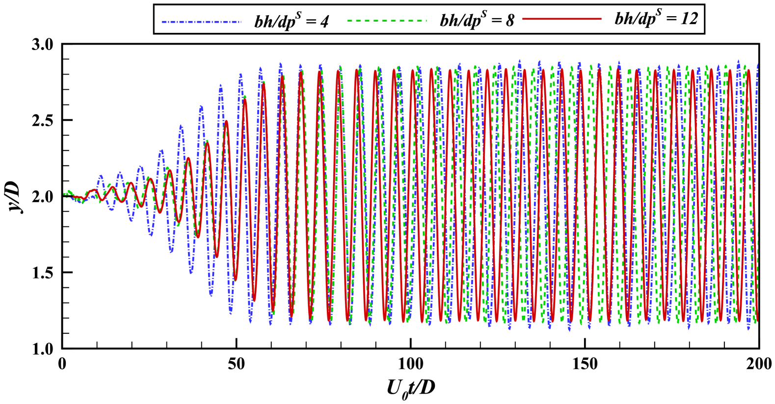
Figure 8: Flow-induced vibration of a beam behind a cylinder: Convergence study of the RKGC method on the amplitude of the displacement in y-direction.

3.3 Dam-break flow through an elastic gate

The third example involves the deformation of an elastic gate subjected to time-dependent water pressure with free-surface flow. As illustrated in Fig. 9, the gate is clamped at its upper end and free at the lower end, interacting with a body of water initially confined in an open-air tank behind it. This setup replicates the experimental study by Antoci et al. [69].

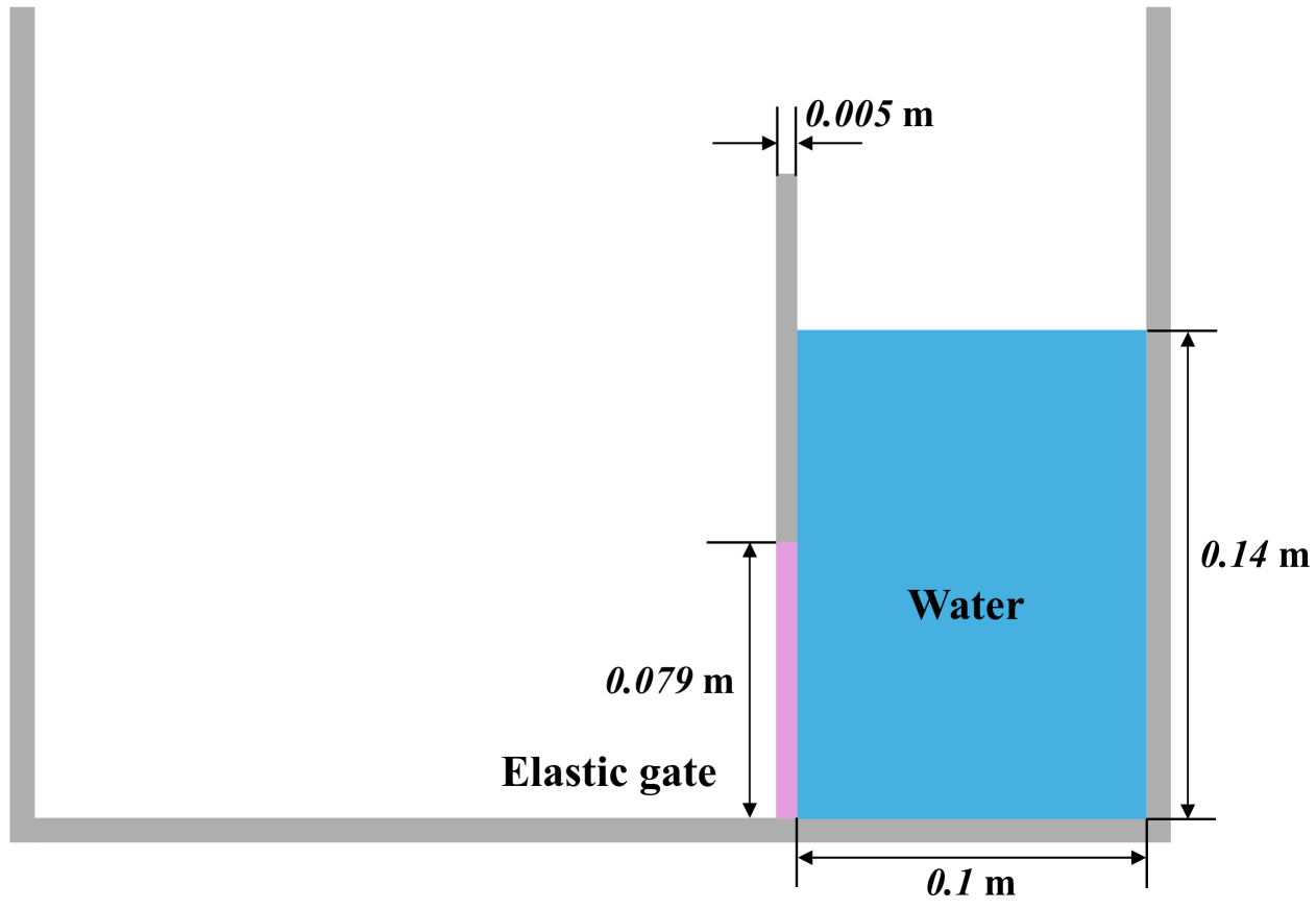
Figure 9: Dam-break flow through an elastic gate: Schematic illustration.

In accordance with Ref. [69], the fluid is treated as inviscid flow with a density of $\rho^{F}=1000~\mathrm{kg/m^{3}}$. The elastic gate, modeled as rubber, follows a linear isotropic material law with a density of $\rho^{S}=~1100\mathrm{kg/m^{3}}$, Young’s modulus $E^{S}=7.8~\mathrm{MPa}$, and Poisson’s ratio $\nu^{S}=0.4$. A clamped boundary condition is enforced at the upper end of the gate via a rigid base constraint.

Fig. 10 compares snapshots from the present RKGC corrected method with experimental frames from Antoci et al. [69] at eight equally spaced time instants.

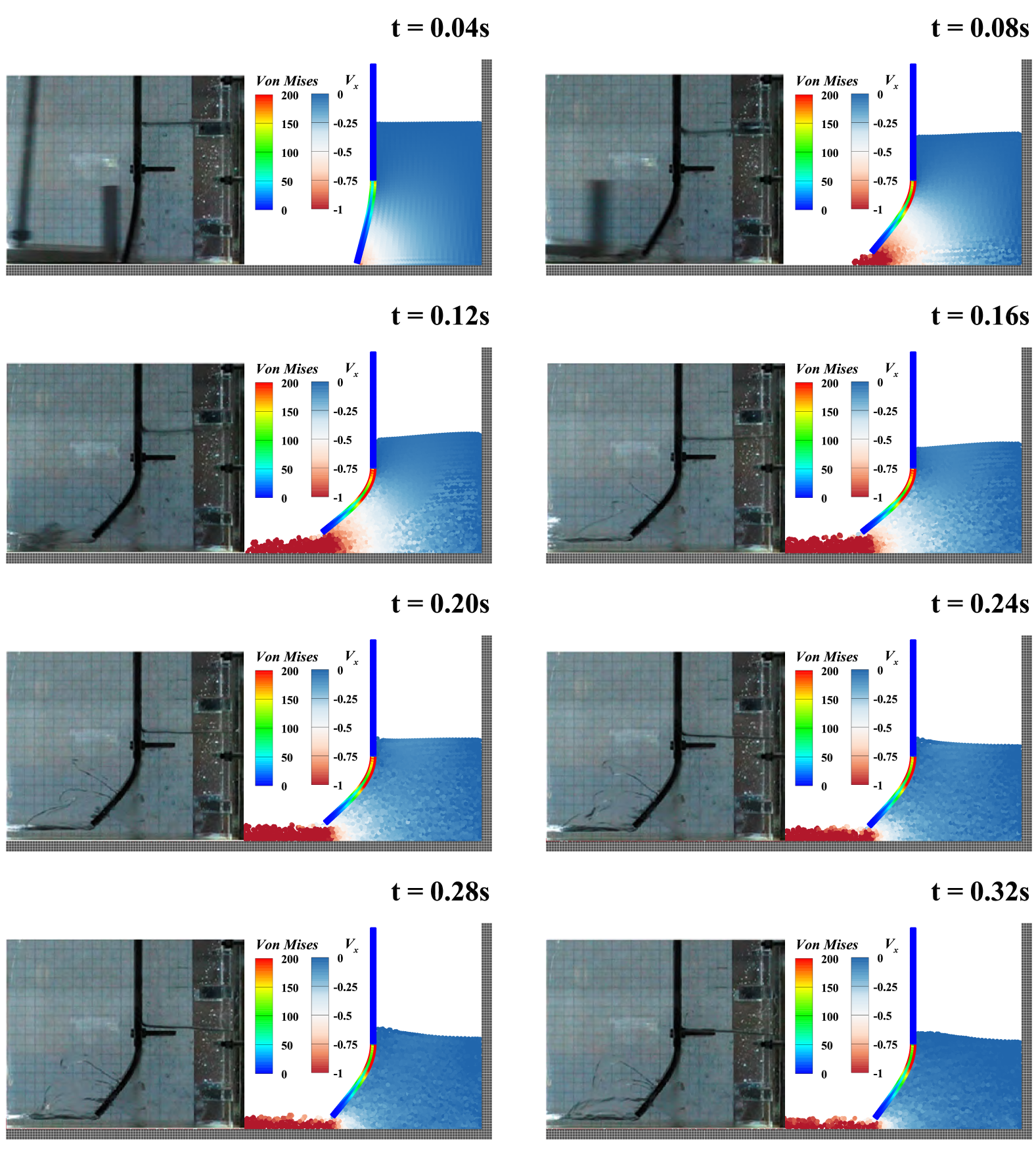
Figure 10: Dam-break flow through an elastic gate: Snapshots from the RKGC method are compared with experimental frames from Antoci et al. [69] at eight equally spaced time instants.

The simulation accurately captures the free-surface motion and closely matches the experimental results. At $t=0.12$ s, the gate exhibits significant deformation, appearing more open than in the experiment. Additionally, side-wall splashes observed experimentally from $t=0.12$ s due to leakage between the tank wall and flexible gate [69, 70] are not reproduced in this two-dimensional simulation.

Fig. 11 compares horizontal and vertical displacements of the gate’s free end from the present simulations with experimental data [69] and numerical results from Khayyer et al. [24], which used the same Poisson’s ratio ($\nu^{S}=0.4$).

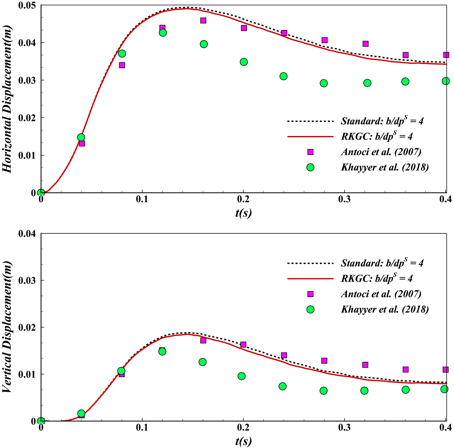
Figure 11: Dam-break flow through an elastic gate: Horizontal (top panel) and vertical (bottom panel) displacement of the free end of the gate obtained by different methods.

Acceptable agreement is observed with both experimental and prior numerical results. During the initial dam-break phase, the horizontal displacement increases rapidly due to high static pressure, with standard and RKGC SPH methods predicting similar gate behavior. At $t=0.15$ s, the gate reaches maximum deformation, where the present RKGC method predicts a displacement closer to experimental measurements. As water recedes and pressure diminishes, the gate gradually returns to equilibrium, governed by elastic forces and dynamic pressure. It is also worth noting that, similar to previous simulations [71, 24, 22], small differences are observed between the present results and the experimental data during the closing phase. These discrepancies can be attributed to the different material model used in simulations [12] and the fact that the selected Poisson’s ratio is lower than that of the actual rubber used in the experiment.

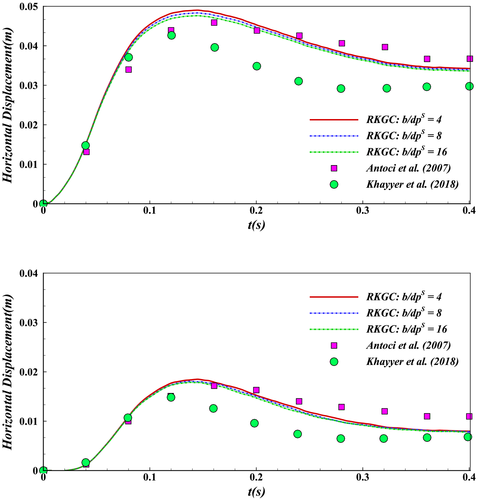
Figure 12: Dam-break flow through an elastic gate: Convergence study of the RKGC method on horizontal (top panel) and vertical (bottom panel) displacement of the free end of the gate.

Although the present method shows slightly larger deviations, convergence studies in Ref. [22] (as shown in their Fig. 11 with $\nu^{S}=0.47$), and that in Fig. 12 for the current case all indicate that the results obtained by the present RKGC method are closer to the converged solution during the gate closing, again confirming the improved numerical accuracy.

3.4 Dam-break flow impacts an elastic plate

The fourth example examines a dam-break flow impacting an elastic plate, as experimentally investigated by Liao et al. [72]. This case involves violent fluid-structure interaction with structural deformations significantly larger than those in Section 3.3, posing considerable computational challenges. The computational setup, shown schematically in Fig. 13, aligns with the experimental configuration from Ref. [72].

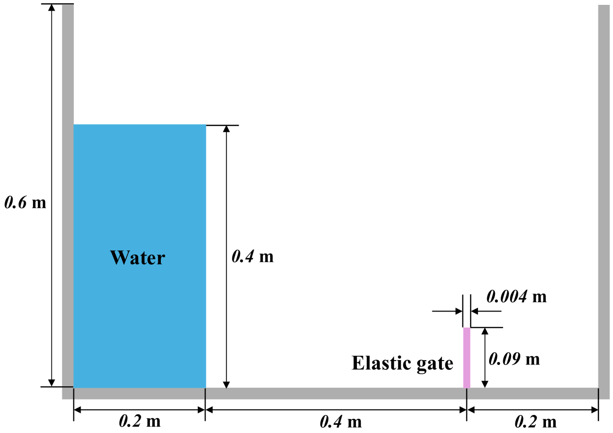
Figure 13: Dam-break flow impacts an elastic plate: Schematic illustration.

The water has a density of $\rho^{F}=998~\mathrm{kg/m^{3}}$ and an initial height of $H=0.4~\mathrm{m}$. The gate material has a density of $\rho^{S}=1161.54~\mathrm{kg/m^{3}}$, Young’s modulus of $E^{S}=3.5~\mathrm{MPa}$, Poisson’s ratio of $\nu^{S}=0.49$, and a thickness of $b=0.004~\mathrm{m}$. The selected particle resolution for the simulation is $b/dp^{S}=4$. Initially, a gate blocks the water; upon release, vertical motion induced by the system rapidly accelerates the gate, generating a dam-break flow that subsequently impacts the elastic plate.

Fig. 14 presents the pressure distribution in the flow field and the von Mises stress of the elastic plate obtained using different methods, compared with an experimental snapshot from Liao et al. [72] at $t=0.35$ s.

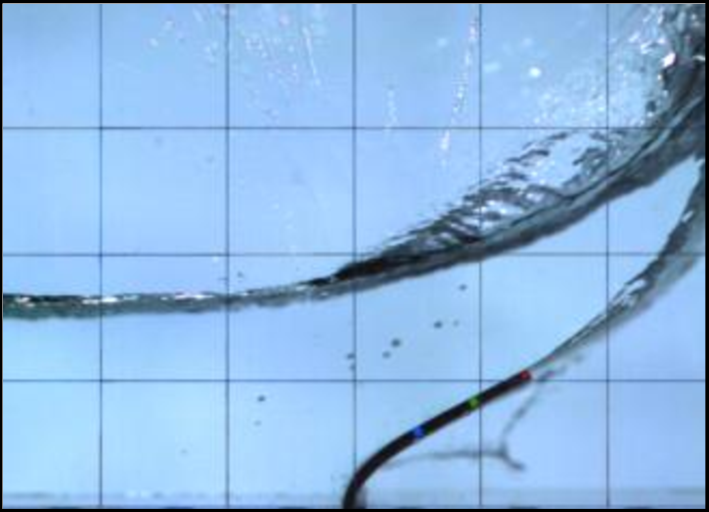
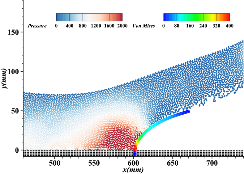
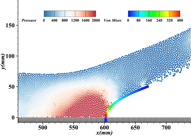
Figure 14: Dam-break flow impacts an elastic plate: Comparison of the pressure distribution in the flow field and deformation of the elastic plate from (a) experimental snapshot captured by Liao et al. [72] and obtained by the (b) Standard SPH method and by the (c) RKGC SPH method at $t=0.35$ s.

Both the standard SPH and RKGC SPH methods produce smooth pressure and stress fields while maintaining stable free surfaces and structural deformations. However, the RKGC SPH method offers superior accuracy, particularly in pressure predictions at the base of the plate. This aligns with the findings of Khayyer et al. [25] (as shown in their Fig. 18) and Xue et al. [48] (as shown in their Fig. 19), where higher pressures were observed in this region. In contrast, the standard SPH method tends to underestimate pressure, highlighting the improved predictive capability of the RKGC approach.

Fig. 15 compares results from the RKGC method with experimental data at four key time instants.

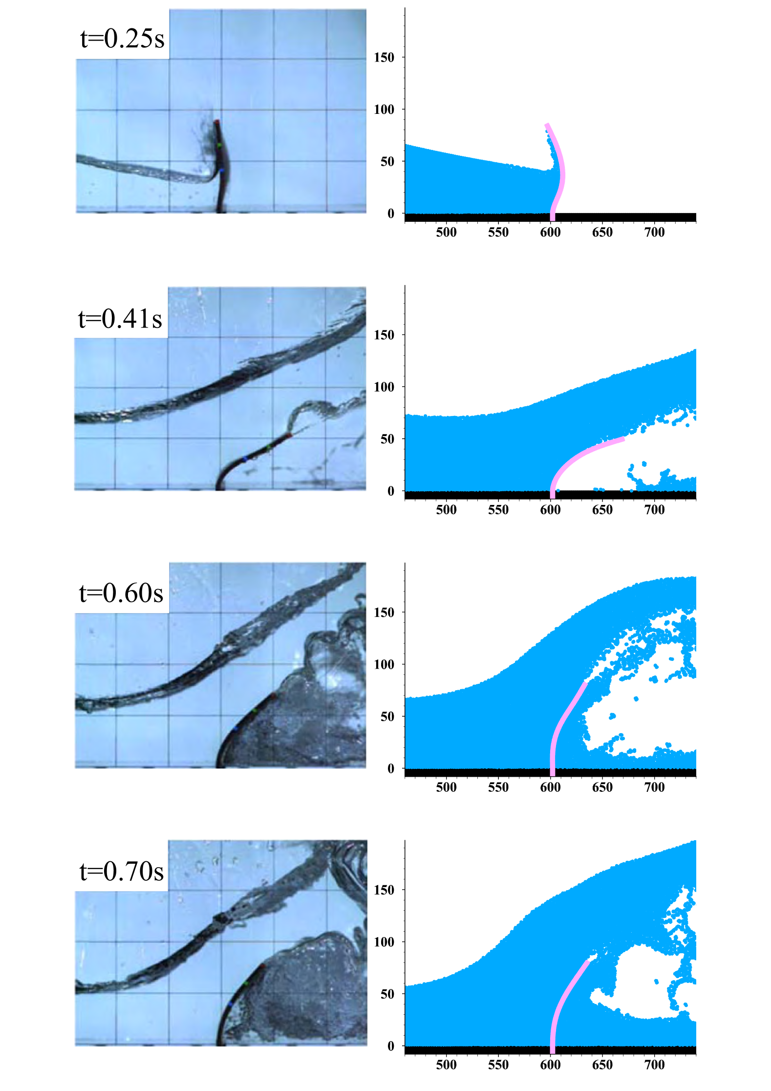
Figure 15: Dam-break flow impacts an elastic plate: Comparison between simulation results obtained by the RKGC method and experimental results [72] at four typical time instants.

Overall, the predicted free surface and elastic plate deformation align well with experimental observations. The experiment reveals that as the fluid impacts the opposite side of the elastic plate, air entrainment leads to significant water spray and cavity formation. This phenomenon is replicated in the simulation, resulting in violent particle splashing. However, some discrepancies arise in the later stages, where fluid-structure interactions become increasingly intense.

Fig. 16 illustrates the time history of the free-end displacement of the elastic plate predicted by the present RKGC method and other reference predictions, compared with experimental measurements.

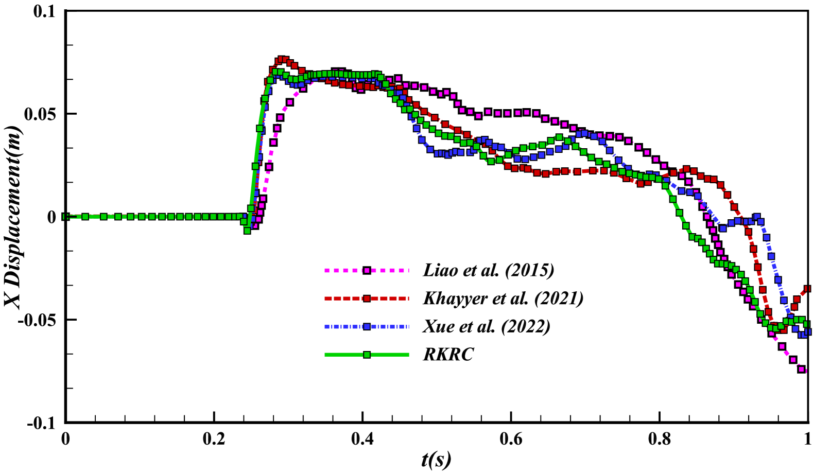
Figure 16: Dam-break flow impacts an elastic plate: Time history of horizontal displacement of free end of the elastic plate.

Similar to other numerical results reported in Refs. [25, 48], the RKGC method closely follows experimental trends. However, as noted in Fig. 15, discrepancies persist in later stages due to the absence of air effects in the current water-structure interaction model. Upon impact, the water jet entraps air, forming cavities that significantly influence the flow field and structural response. This limitation is well-documented Refs. [25, 65], suggesting that incorporating multi-phase air-water-structure simulations would enhance the accuracy of deformation predictions in future studies.

3.5 Sloshing in a rolling tank with a elastic baffle

Finally, the proposed RKGC method is validated using a rolling tank example, where an elastic baffle is clamped at the bottom. Following the experimental setup performed by Idelsohn et al. [73], the computational configuration is illustrated in Fig. 17.

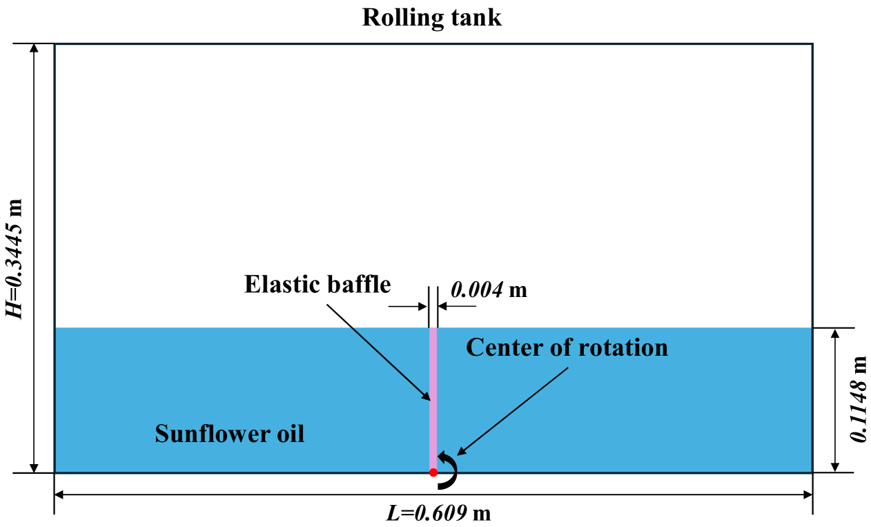
Figure 17: Sloshing in a rolling tank with a elastic baffle: Schematic illustration.

The tank, measuring $0.609\times 0.3445$ m, is filled with sunflower oil to a height of $0.1148$ m. The density and kinematic viscosity of the oil are $\rho^{F}=917\ \mathrm{kg/m^{3}}$ and $\mu^{F}=5.0\times 10^{-5}\ \mathrm{m^{2}/s}$, respectively. An elastic baffle made of electrolyte polyurethane is clamped at the bottom center of the tank, with its height matching the liquid level. The baffle has a thickness of $b=0.004$ m and a density of $\rho^{S}=1100\ \mathrm{kg/m^{3}}$. Its mechanical properties include Young’s modulus of $E^{S}=6.0\mathrm{MPa}$ and a Poisson’s ratio of $\nu^{S}=0.49$. The tank undergoes rolling motion about its bottom center with a maximum amplitude of $4^{\circ}$ and a period of 1.211 s. A sensor at the free end of the baffle tracks the horizontal displacement. Simulations use the particle spacing ratio of $b/dp^{S}=4$.

Fig. 18 compares time history of the baffle’s horizontal displacement from the present method with experimental data [73] and numerical results from Khayyer et al. [25] and Xu et al. [48].

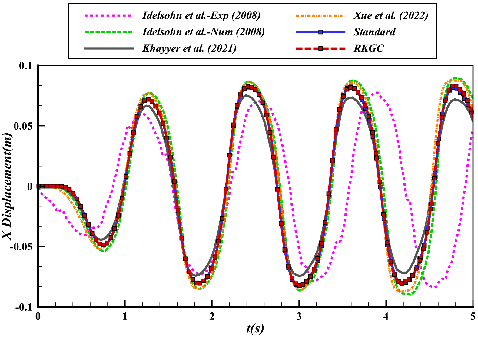
Figure 18: Sloshing in a rolling tank with a elastic baffle: Time history of free end horizontal displacement of the elastic baffle .

After an initial transient phase, the baffle exhibits regular oscillations with stable amplitude and period. Both standard and RKGC SPH methods align with reference results in amplitude and frequency, validating the good accuracy of the RKGC method. However, observed discrepancies in swing period frequency, also noted in Refs. [73, 48], may stem from the inertial effects.

Fig. 19 presents snapshots of the sloshing behavior in the rolling tank with the elastic baffle obtained using the RKGC method. These are compared with experimental observations from Ref. [73] at $t=1.84$ s, $2.12$ s, $2.32$ s and $2.56$ s.

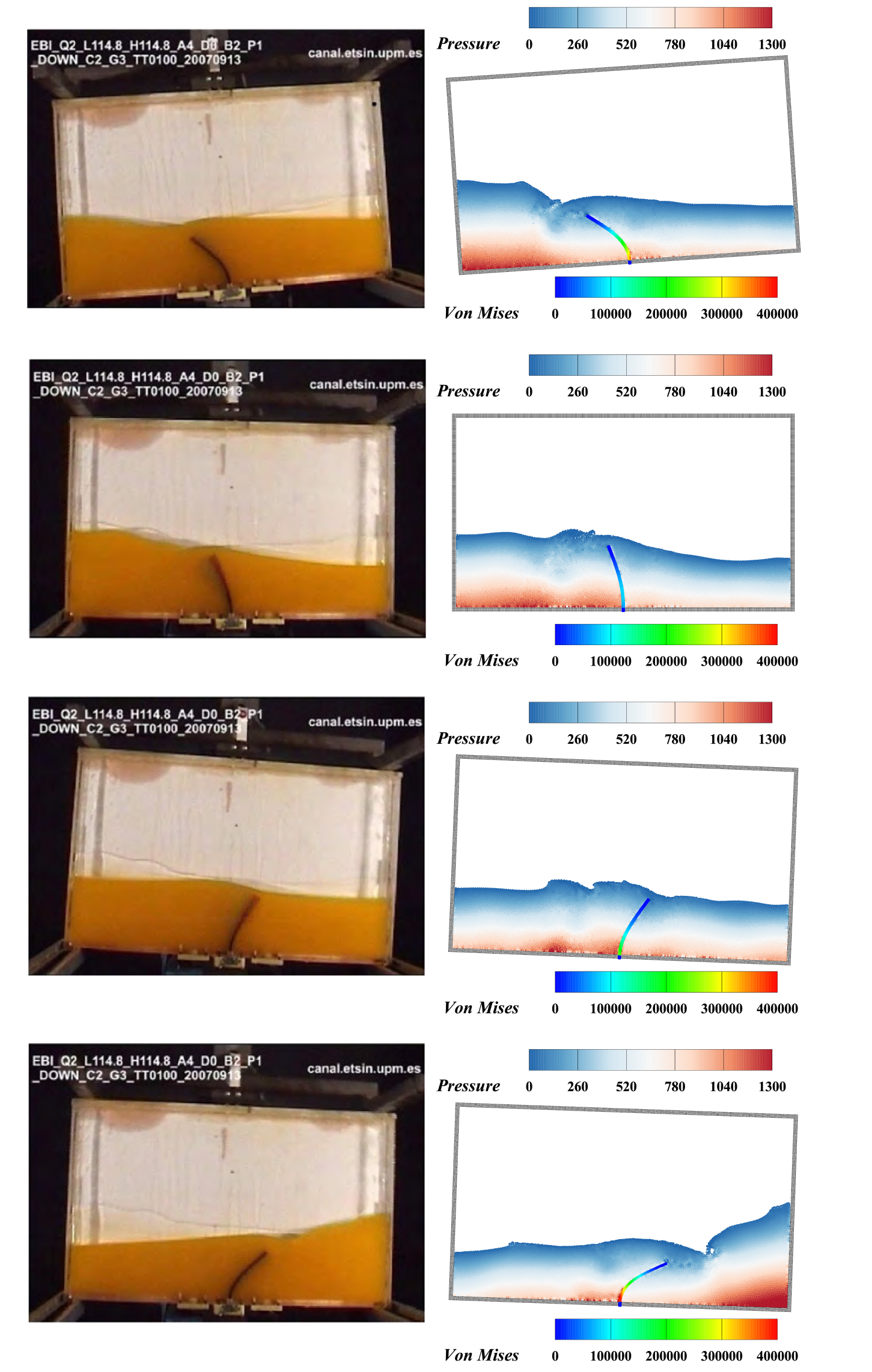
Figure 19: Sloshing in a rolling tank with a elastic baffle: Comparison between simulation results obtained by the RKGC method and experimental results [73] at $t=1.84$ s, $2.12$ s, $2.32$ s and $2.56$ s.

The elastic baffle effectively isolates the pressure field within the liquid, serving as a dynamic motion boundary. Its presence also disrupts the free surface, leading to an irregular morphology. The comparison of numerical and experimental results at various time intervals show strong agreement in both the free surface shape and structural deformation, further validating the accuracy of the proposed numerical model.

4 Conclusion and remark

From the perspective of fluid-structure interaction (FSI) challenges, this study introduces a corrected Riemann SPH method for the fluid domain to enhance numerical accuracy in multi-resolution FSI simulations. Integrated with the RKGC formulation, which ensures second-order convergence and first-order consistency in SPH approximations, the fluid domain is solved with the corrected Riemann SPH method, which plays a significant role in multi-resolution FSI analysis, where the fluid domain generally has low resolutions. Validation across various FSI cases confirms that the proposed RKGC-corrected Riemann SPH method improves accuracy and ensures robust convergence. Future efforts will focus on refining fluid-solid interaction treatments and extending high-order consistency corrections to the solid phase. Addressing these aspects will further establish SPH as a versatile, efficient, and high-fidelity tool for modeling complex FSI phenomena in engineering applications.

Author Declarations

The authors have no conflicts to disclose.

References

- [1] E. H. Dowell, K. C. Hall, Modeling of fluid-structure interaction, Annual review of fluid mechanics 33 (1) (2001) 445–490.
- [2] H.-J. Bungartz, M. Schäfer, Fluid-structure interaction: modelling, simulation, optimisation, Vol. 53, Springer Science & Business Media, 2006.
- [3] M. Liu, Z. Zhang, Smoothed particle hydrodynamics (sph) for modeling fluid-structure interactions, Science China Physics, Mechanics & Astronomy 62 (2019) 1–38.
- [4] T. E. Tezduyar, M. Behr, S. Mittal, J. Liou, A new strategy for finite element computations involving moving boundaries and interfaces—the deforming-spatial-domain/space-time procedure: Ii. computation of free-surface flows, two-liquid flows, and flows with drifting cylinders, Computer methods in applied mechanics and engineering 94 (3) (1992) 353–371.
- [5] C. S. Peskin, The immersed boundary method, Acta numerica 11 (2002) 479–517.
- [6] C. W. Hirt, B. D. Nichols, Volume of fluid (vof) method for the dynamics of free boundaries, Journal of computational physics 39 (1) (1981) 201–225.
- [7] S. Osher, J. A. Sethian, Fronts propagating with curvature-dependent speed: Algorithms based on hamilton-jacobi formulations, Journal of computational physics 79 (1) (1988) 12–49.
- [8] L. B. Lucy, A numerical approach to the testing of the fission hypothesis, Astronomical Journal, vol. 82, Dec. 1977, p. 1013-1024. 82 (1977) 1013–1024.
- [9] R. A. Gingold, J. J. Monaghan, Smoothed particle hydrodynamics: theory and application to non-spherical stars, Monthly notices of the royal astronomical society 181 (3) (1977) 375–389.
- [10] B. Mishra, R. K. Rajamani, The discrete element method for the simulation of ball mills, Applied Mathematical Modelling 16 (11) (1992) 598–604.
- [11] S. Koshizuka, Y. Oka, Moving-particle semi-implicit method for fragmentation of incompressible fluid, Nuclear science and engineering 123 (3) (1996) 421–434.
- [12] Q. Yang, V. Jones, L. McCue, Free-surface flow interactions with deformable structures using an sph–fem model, Ocean engineering 55 (2012) 136–147.
- [13] C. Chen, W.-K. Shi, Y.-M. Shen, J.-Q. Chen, A.-M. Zhang, A multi-resolution sph-fem method for fluid–structure interactions, Computer Methods in Applied Mechanics and Engineering 401 (2022) 115659.
- [14] D. Hu, T. Long, Y. Xiao, X. Han, Y. Gu, Fluid–structure interaction analysis by coupled fe–sph model based on a novel searching algorithm, Computer Methods in Applied Mechanics and Engineering 276 (2014) 266–286.
- [15] Z. Li, J. Leduc, J. Nunez-Ramirez, A. Combescure, J.-C. Marongiu, A non-intrusive partitioned approach to couple smoothed particle hydrodynamics and finite element methods for transient fluid-structure interaction problems with large interface motion, Computational Mechanics 55 (2015) 697–718.
- [16] Y. Zhang, D. Wan, Mps-fem coupled method for fluid–structure interaction in 3d dam-break flows, International Journal of Computational Methods 16 (02) (2019) 1846009.
- [17] X. Chen, Y. Zhang, D. Wan, Numerical study of 3-d liquid sloshing in an elastic tank by mps-fem coupled method, Journal of Ship Research 63 (03) (2019) 143–153.
- [18] G. Oger, P.-M. Guilcher, E. Jacquin, L. Brosset, J.-B. Deuff, D. Le Touzé, Simulations of hydro-elastic impacts using a parallel sph model, in: ISOPE International Ocean and Polar Engineering Conference, ISOPE, 2009, pp. ISOPE–I.
- [19] M.-b. Liu, J.-r. Shao, H.-q. Li, Numerical simulation of hydro-elastic problems with smoothed particle hydrodynamics method, Journal of Hydrodynamics 25 (5) (2013) 673–682.
- [20] L. Han, X. Hu, Sph modeling of fluid-structure interaction, Journal of Hydrodynamics 30 (2018) 62–69.
- [21] P. Sun, D. Le Touzé, A.-M. Zhang, Study of a complex fluid-structure dam-breaking benchmark problem using a multi-phase sph method with apr, Engineering Analysis with Boundary Elements 104 (2019) 240–258.
- [22] C. Zhang, M. Rezavand, X. Hu, A multi-resolution sph method for fluid-structure interactions, Journal of Computational Physics 429 (2021) 110028.
- [23] Z.-F. Meng, A.-M. Zhang, J.-L. Yan, P.-P. Wang, A. Khayyer, A hydroelastic fluid–structure interaction solver based on the riemann-sph method, Computer Methods in Applied Mechanics and Engineering 390 (2022) 114522.
- [24] A. Khayyer, H. Gotoh, H. Falahaty, Y. Shimizu, An enhanced isph–sph coupled method for simulation of incompressible fluid–elastic structure interactions, Computer Physics Communications 232 (2018) 139–164.
- [25] A. Khayyer, Y. Shimizu, H. Gotoh, S. Hattori, Multi-resolution isph-sph for accurate and efficient simulation of hydroelastic fluid-structure interactions in ocean engineering, Ocean Engineering 226 (2021) 108652.
- [26] S.-C. Hwang, J.-C. Park, H. Gotoh, A. Khayyer, K.-J. Kang, Numerical simulations of sloshing flows with elastic baffles by using a particle-based fluid–structure interaction analysis method, Ocean Engineering 118 (2016) 227–241.
- [27] A. Khayyer, N. Tsuruta, Y. Shimizu, H. Gotoh, Multi-resolution mps for incompressible fluid-elastic structure interactions in ocean engineering, Applied Ocean Research 82 (2019) 397–414.
- [28] P. Randles, L. D. Libersky, Smoothed particle hydrodynamics: some recent improvements and applications, Computer methods in applied mechanics and engineering 139 (1-4) (1996) 375–408.
- [29] W. K. Liu, S. Jun, Y. F. Zhang, Reproducing kernel particle methods, International journal for numerical methods in fluids 20 (8-9) (1995) 1081–1106.
- [30] W. K. Liu, S. Jun, S. Li, J. Adee, T. Belytschko, Reproducing kernel particle methods for structural dynamics, International Journal for Numerical Methods in Engineering 38 (10) (1995) 1655–1679.
- [31] J. Chen, J. Beraun, T. Carney, A corrective smoothed particle method for boundary value problems in heat conduction, International Journal for Numerical Methods in Engineering 46 (2) (1999) 231–252.
- [32] M. Liu, G.-R. Liu, Restoring particle consistency in smoothed particle hydrodynamics, Applied numerical mathematics 56 (1) (2006) 19–36.
- [33] R. Batra, G. Zhang, Analysis of adiabatic shear bands in elasto-thermo-viscoplastic materials by modified smoothed-particle hydrodynamics (msph) method, Journal of computational physics 201 (1) (2004) 172–190.
- [34] G. Zhang, R. Batra, Modified smoothed particle hydrodynamics method and its application to transient problems, Computational mechanics 34 (2) (2004) 137–146.
- [35] S. Sibilla, An algorithm to improve consistency in smoothed particle hydrodynamics, Computers & Fluids 118 (2015) 148–158.
- [36] A. M. Nasar, G. Fourtakas, S. J. Lind, J. King, B. D. Rogers, P. K. Stansby, High-order consistent sph with the pressure projection method in 2-d and 3-d, Journal of Computational Physics 444 (2021) 110563.
- [37] S. N. Atluri, J. Cho, H.-G. Kim, Analysis of thin beams, using the meshless local petrov–galerkin method, with generalized moving least squares interpolations, Computational mechanics 24 (5) (1999) 334–347.
- [38] N. Flyer, B. Fornberg, Radial basis functions: Developments and applications to planetary scale flows, Computers & Fluids 46 (1) (2011) 23–32.
- [39] J. King, S. J. Lind, A. M. Nasar, High order difference schemes using the local anisotropic basis function method, Journal of Computational Physics 415 (2020) 109549.
- [40] N. Trask, M. Perego, P. Bochev, A high-order staggered meshless method for elliptic problems, SIAM Journal on Scientific Computing 39 (2) (2017) A479–A502.
- [41] R. Vignjevic, J. R. Reveles, J. Campbell, Sph in a total lagrangian formalism, CMC-Tech Science Press- 4 (3) (2006) 181.
- [42] J. P. Vila, Sph renormalized hybrid methods for conservation laws: applications to free surface flows, in: Meshfree methods for partial differential equations II, Springer, 2005, pp. 207–229.
- [43] V. Zago, L. J. Schulze, G. Bilotta, N. Almashan, R. Dalrymple, Overcoming excessive numerical dissipation in sph modeling of water waves, Coastal Engineering 170 (2021) 104018.
- [44] G. Liang, X. Yang, Z. Zhang, G. Zhang, Study on the propagation of regular water waves in a numerical wave flume with the -sphc model, Applied Ocean Research 135 (2023) 103559.
- [45] G. Oger, M. Doring, B. Alessandrini, P. Ferrant, An improved sph method: Towards higher order convergence, Journal of Computational Physics 225 (2) (2007) 1472–1492.
- [46] X. Huang, P. Sun, H. Lü, S. Zhong, Development of a numerical wave tank with a corrected smoothed particle hydrodynamics scheme to reduce nonphysical energy dissipation, Chinese Journal of Theoretical and Applied Mechanics 54 (6) (2022) 1502–1515.
- [47] B. Zhang, N. Adams, X. Hu, Towards high-order consistency and convergence of conservative sph approximations, Computer Methods in Applied Mechanics and Engineering 433 (2025) 117484.
- [48] B. Xue, S.-P. Wang, Y.-X. Peng, A.-M. Zhang, A novel coupled riemann sph–rkpm model for the simulation of weakly compressible fluid–structure interaction problems, Ocean Engineering 266 (2022) 112447.
- [49] J. P. Morris, P. J. Fox, Y. Zhu, Modeling low reynolds number incompressible flows using sph, Journal of computational physics 136 (1) (1997) 214–226.
- [50] C. Zhang, X. Hu, N. A. Adams, A weakly compressible sph method based on a low-dissipation riemann solver, Journal of Computational Physics 335 (2017) 605–620.
- [51] C. Zhang, Y. Zhu, X. Hu, An efficient multi-resolution sph framework for multi-phase fluid-structure interactions, Science China Physics, Mechanics & Astronomy 66 (10) (2023) 104712.
- [52] C. Zhang, Y.-j. Zhu, D. Wu, N. A. Adams, X. Hu, Smoothed particle hydrodynamics: Methodology development and recent achievement, Journal of Hydrodynamics 34 (5) (2022) 767–805.
- [53] I. S. Sokolnikoff, Mathematical theory of elasticity (1946).
- [54] C. Zhang, M. Rezavand, X. Hu, Dual-criteria time stepping for weakly compressible smoothed particle hydrodynamics, Journal of Computational Physics 404 (2020) 109135.
- [55] Y. Ren, P. Lin, C. Zhang, X. Hu, An efficient correction method in riemann sph for the simulation of general free surface flows, Computer Methods in Applied Mechanics and Engineering 417 (2023) 116460.
- [56] Y. Zhu, C. Zhang, Y. Yu, X. Hu, A cad-compatible body-fitted particle generator for arbitrarily complex geometry and its application to wave-structure interaction, Journal of Hydrodynamics 33 (2) (2021) 195–206.
- [57] J. J. Monaghan, Smoothed particle hydrodynamics, Annual review of astronomy and astrophysics 30 (1) (1992) 543–574.
- [58] H.-G. Lyu, P.-N. Sun, P.-Z. Liu, X.-T. Huang, A. Colagrossi, Derivation of an improved smoothed particle hydrodynamics model for establishing a three-dimensional numerical wave tank overcoming excessive numerical dissipation, Physics of Fluids 35 (6) (2023).
- [59] G. Fourey, C. Hermange, D. Le Touzé, G. Oger, An efficient fsi coupling strategy between smoothed particle hydrodynamics and finite element methods, Computer Physics Communications 217 (2017) 66–81.
- [60] A. Khayyer, Y. Shimizu, T. Gotoh, H. Gotoh, Enhanced resolution of the continuity equation in explicit weakly compressible sph simulations of incompressible free-surface fluid flows, Applied Mathematical Modelling 116 (2023) 84–121.
- [61] T. Bao, J. Hu, S. Wang, C. Huang, Y. Yu, A. Shakibaeinia, An entirely sph-based fsi solver and numerical investigations on hydrodynamic characteristics of the flexible structure with an ultra-thin characteristic, Computer Methods in Applied Mechanics and Engineering 431 (2024) 117255.
- [62] Y. Zhu, C. Zhang, X. Hu, A dynamic relaxation method with operator splitting and random-choice strategy for sph, Journal of Computational Physics 458 (2022) 111105.
- [63] A. Khayyer, H. Gotoh, S. Shao, Enhanced predictions of wave impact pressure by improved incompressible sph methods, Applied Ocean Research 31 (2) (2009) 111–131.
- [64] S. Turek, J. Hron, Proposal for numerical benchmarking of fluid-structure interaction between an elastic object and laminar incompressible flow, Springer, 2006.
- [65] P.-N. Sun, D. Le Touze, G. Oger, A.-M. Zhang, An accurate fsi-sph modeling of challenging fluid-structure interaction problems in two and three dimensions, Ocean Engineering 221 (2021) 108552.
- [66] R. Bhardwaj, R. Mittal, Benchmarking a coupled immersed-boundary-finite-element solver for large-scale flow-induced deformation, AIAA journal 50 (7) (2012) 1638–1642.
- [67] H. Zheng, H. Qiang, Y. Zhu, C. Zhang, A parameter-free particle relaxation technique for smoothed particle hydrodynamics, Physics of Fluids 36 (9) (2024).
- [68] F.-B. Tian, H. Dai, H. Luo, J. F. Doyle, B. Rousseau, Fluid–structure interaction involving large deformations: 3d simulations and applications to biological systems, Journal of computational physics 258 (2014) 451–469.
- [69] C. Antoci, M. Gallati, S. Sibilla, Numerical simulation of fluid–structure interaction by sph, Computers & structures 85 (11-14) (2007) 879–890.
- [70] A. Rafiee, K. P. Thiagarajan, An sph projection method for simulating fluid-hypoelastic structure interaction, Computer Methods in Applied Mechanics and Engineering 198 (33-36) (2009) 2785–2795.
- [71] Z. Zhang, T. Long, J. Chang, M. Liu, A smoothed particle element method (spem) for modeling fluid–structure interaction problems with large fluid deformations, Computer Methods in Applied Mechanics and Engineering 356 (2019) 261–293.
- [72] K. Liao, C. Hu, M. Sueyoshi, Free surface flow impacting on an elastic structure: Experiment versus numerical simulation, Applied Ocean Research 50 (2015) 192–208.
- [73] S. Idelsohn, J. Marti, A. Souto-Iglesias, E. Onate, Interaction between an elastic structure and free-surface flows: experimental versus numerical comparisons using the pfem, Computational Mechanics 43 (2008) 125–132.