A quantile-based bivariate distribution

Abstract

In this paper we present a flexible bivariate distribution specified by a quantile function. The distribution contains as special cases new bivariate exponential, Pareto I, Pareto II, beta, power, log logistic and uniform distributions and also can approximate many other continuous models. Various $L$-moment based properties of the distribution such as covariance, coskewness, cokurtosis, $L$-correlation, etc are discussed. The distribution is used to model two real data sets.

1 Introduction

Quantile functions play the same role as distribution functions, they being equivalent representations of one another and so quantile functions have applications in all problems where distribution functions are useful. Although generally a quantile function is defined as the inverse of the distribution function and obtained in this way on many occasions, several distributions are defined in terms of quantile functions independently of the form of the distribution function as a left continuous, non-decreasing function on the unit interval, $I=[0,1]$. Examples of such distributions are the lambda distributions and its variants, Wakeby, power-Pareto, Govindarajulu, Kamps, linear mean residual quantile function models etc. See Nair and Vineshkumar, (2022) for details. The popularity of such quantile forms arises in model building from the fact that they provide satisfactory approximations for a wide variety of data, have simple algebraic structure, easy to use in generating random samples in simulation studies and often estimates based on them are more robust than their counterparts derived from distribution functions. Moreover simple algebraic operations like addition, multiplication and monotone transformations on quantile functions lead to more general models which are quiet handy in data analysis problems.

There is an alternative route by which quantile-based distributions can be visited by writing the density function in terms of the distribution function. A general discussion on the class of distributions defined by the relationship between the density and distribution functions initiated in Jones, (2007) points out the members of this class and their properties. It is pointed out that the distribution of order statistics belongs to this class, see Jones, (2004) and the discussions on this paper. Special properties of the distribution of order statistics of some specified distributions can also be seen in Kamps, (1991), Balakrishnan and Akhundov, (2003) and Akhundov et al., (2004).

Inspite of the utility of quantile functions in analyzing univariate data is well established, the progress of similar approaches in the multivariate case has been slow. Some attempts made by researchers like Chen and Welsh, (2002), Belzunce et al., (2007) and Cai, (2010) to extend the concept of quantiles to higher dimensions, were not directed towards suggesting multivariate quantile functions that can specify distributions as in the univariate case. Conceiving the bivariate quantile function as a pair that transforms the points in the unit square $I^{2}$ to points in the $x_{1}-x_{2}$ plane, in the same way as I is transformed to $\mathbb{R}$ in the univariate cases, Vineshkumar and Nair, (2019) and Nair and Vineshkumar, (2023) find bivariate quantile function of distributions in $\mathbb{R}_{2}$. They have pointed out the basic properties of these functions and their applications as model of bivariate lifetime data. In the process some bivariate distributions generated by quantile functions were also presented.

The main objective of the present work is to propose a flexible bivariate distribution arising from a bivariate quantile function, that can represent different types of data in a unified framework. The proposed distribution subsumes some new bivariate exponential, Pareto, power, log logistic, etc as special cases and many other quantile functions with special properties as other members. With its flexibility it can serve as a black box model of random phenomena in a wide range of cases. A method of inferring the parameters with real data illustrations also form part of this work.

The work is organized into five sections. In the next section we introduce the model and deduce its special cases . This is followed in Section 3 by discussing the properties of the model including covariance, coskewness, cokurtosis and measures of dependence. The application of the model in two real data situations is demonstrated in Section 4. The paper ends with Section 5 in the form of a short conclusion.

2 The bivariate distribution

We consider a random vector $\left(X_{1},X_{2}\right)$ with absolutely continuous distribution function, $F\left(x_{1},x_{2}\right)$ and survival function $\bar{F}\left(x_{1},x_{2}\right)$. Then the bivariate quantile function of $\left(X_{1},X_{2}\right)$ is defined with respect to the marginal distribution function $F_{1}\left(x_{1}\right)$ of $X_{1}$ and the conditional distribution function $F_{21}\left(x_{2}\mid x_{1}\right)=P\left(X_{2}\leq x_{1}\mid X_{1}>x_{1}\right)$ as the pair $\left(Q_{1}\left(u_{1}\right),Q_{21}\left(u_{1},u_{2}\right)\right)$ where

$$Q_{1}\left(u_{1}\right)=\inf\left[x_{1}\mid F\left(x_{1}\right)\geq u_{1}\right],\quad 0\leq u_{1}\leq 1$$

and

$$Q_{21}\left(u_{1},u_{2}\right)=\inf\left[x_{2}\mid F_{21}\left(x_{2}\mid Q_{1}\right)\geq u_{2}\right],\quad 0\leq u_{2}\leq 1.$$

The bivariate survival function of $\left(X_{1},X_{2}\right)$ is recovered from $\left(Q_{1},Q_{21}\right)$ as

$$\bar{F}\left(x_{1},x_{2}\right)=\bar{F}_{1}\left(x_{1}\right)\bar{F}_{21}\left(x_{2}\mid x_{1}\right)=P\left(X_{1}\geq x_{1}\right)P\left(X_{2}>x_{1}\mid X_{1}>x_{1}\right),$$

where $F_{1}\left(x_{1}\right)=\inf\left[u_{1}\mid Q_{1}\left(u_{1}\right)\geq x_{1}\right]$ and $F_{21}\left(x_{2}\mid x_{1}\right)=\inf\left[u_{2}\mid Q_{21}\left(u_{1},u_{2}\right)\geq x_{2}\right]$. Further the quantile density functions $q_{1}\left(u_{1}\right)=\frac{dQ_{1}}{du_{1}}$ and $q_{21}\left(u_{1},u_{2}\right)=\frac{\partial Q_{21}}{\partial u_{2}}$ also determine the distribution of $\left(X_{1},X_{2}\right)$ uniquely.

The bivariate distribution defined in this work is characterized by the pair $\left(q_{1}(u_{1}),q_{21}(u_{1},u_{2})\right)$ where

$$q_{1}\left(u_{1}\right)=c_{1}u_{1}^{\alpha_{1}}\left(1-u_{1}\right)^{\beta_{1}}$$ (2.1)

and

$$q_{21}\left(u_{1},u_{2}\right)=c_{2}\left(1+\theta u_{1}\right)u_{2}^{\alpha_{2}}\left(1-u_{2}\right)^{\beta_{2}},$$ (2.2)

where $c_{1},c_{2}>0,\ \theta\geq 0$ and $\alpha_{i}$ and $\beta_{i}$ are real parameters, $i=1,2$. As $u_{1}\rightarrow 0$ in $q_{21}$, $q_{2}\left(u_{2}\right)=c_{2}u_{2}^{\alpha_{2}}\left(1-u_{2}\right)^{\beta_{2}}$ represents the marginal distribution of $X_{2}$.

An attractive aspect of the model in (2.1) and (2.2) is that it gives many tractable distributions as special cases, that have different shapes and properties that makes it a highly flexible family.

Case (i): $\alpha_{i},\beta_{i}>-1$.

In this case we have

$$Q_{i}\left(u_{i}\right)=C_{i}B_{u_{i}}\left(\alpha_{i}+1,\beta_{i}+1\right),\quad i=1,2$$ (2.3)

and

$$Q_{21}\left(u_{1},u_{2}\right)=C_{2}\left(1+\theta u_{1}\right)B_{u_{2}}\left(\alpha_{2}+1,\beta_{2}+1\right),$$ (2.4)

where $B_{x}(m,n)=\int_{0}^{x}t^{m-1}(1-t)^{n-1}dt$ is the incomplete beta function. Note that $C_{i}=\frac{1}{B\left(\alpha_{i}+1,\beta_{i}+1\right)}$, so that (2.4) is the incomplete beta function ratio $I_{u}\left(\alpha_{i}+1,\beta_{i}+1\right)=$ $\frac{B_{u}\left(\alpha_{i}+1,\beta_{i}+1\right)}{B\left(\alpha_{i}+1,\beta_{i}+1\right)}.$ Hence the distribution function of $X_{i}$ is the inverse, $I^{-1}_{u_{i}}\left(\alpha_{i}+1,\beta_{i}+1\right)$, of the incomplete beta function ratio with support $[0,1]$. This distribution called the complementary beta distribution has been studied in Jones, (2002). For purposes of computation, $F_{X_{i}}\left(u_{i}\right)=I^{-1}_{u_{i}}\left(\alpha_{i}+1,\beta_{i}+1\right)$ is available in tabular form in packages as inv inc beta $(a,b)$. The conditional distribution $F_{21}$ is also of the same form with

$$F_{X_{2}\mid Q_{1}}\left(x_{2}\right)=x_{2}\frac{I^{-1}_{u_{2}}\left(\alpha_{2}+1,\beta_{2}+1\right)}{\left(1+\theta u_{1}\right)}.$$

We name the bivariate distributions in this paper according to the form of the marginals and accordingly when $\alpha_{i}>-1,\ \beta_{i}>-1$ we have a bivariate complementary beta distribution with support $I^{2}$.

Case (ii): $\beta_{i}=0$.

We have $q_{1}\left(u_{1}\right)=c_{1}u_{1}^{\alpha_{1}};\quad q_{21}=c_{2}\left(1+\theta u_{1}\right)u_{2}^{\alpha_{2}},$

$$\Rightarrow Q_{1}\left(u_{1}\right)=\frac{c_{1}u_{1}^{\alpha_{1}+1}}{\alpha_{1}+1};\quad Q_{21}\left(u_{1},u_{2}\right)=\frac{c_{2}\left(1+\theta u_{1}\right)u_{2}^{\alpha_{2}+1}}{\alpha_{2}+1},$$

$$\Rightarrow F_{1}\left(x_{1}\right)=\left(\frac{x_{1}}{b_{1}}\right)^{a_{1}};\quad F_{21}\left(x_{2}\mid x_{1}\right)=\left(\frac{x_{2}}{\left(1+\theta u_{1}\right)b_{2}}\right)^{a_{2}},$$

where $a_{i}=\left(\alpha_{i}+1\right)^{-1}>0;\quad b_{i}=\frac{c_{i}}{\alpha_{1}+1}>0;\quad u_{1}=F_{1}\left(x_{1}\right)$.

$$\Rightarrow\bar{F}\left(x_{1},x_{2}\right)=\left(1-\left(\frac{x_{1}}{b_{1}}\right)^{a_{1}}\right) \left(1-\left(1+\theta\left(\frac{x_{1}}{b_{1}}\right)^{a_{1}}\right)^{-a_{2}}\left(\frac{x_{2}}{b_{2}}\right)^{a_{2}}\right),$$ (2.5)

$$0\leq x_{i}\leq b_{i};\quad a_{i},b_{i}>0.$$

Equation (2.5) represents a bivariate power distribution with marginals $F_{i}\left(x_{i}\right)=\left(\frac{x_{i}}{b_{i}}\right)^{a_{i}},$ $0\leq x_{i}\leq b_{i};\ a_{i}>0;\ b_{i}>0$. When $a_{i}=1$, that is $\alpha_{i}=0$ the special case of a bivariate uniform distribution $\bar{F}\left(x_{1},x_{2}\right)=\left(1-\frac{x_{1}}{b_{1}}\right)\left(1-\frac{x_{2}}{b_{2}\left(1+\theta\frac{x_{1}}{a_{1}}\right)}\right)$ is obtained. In the above case $b_{i}>0\Rightarrow\alpha_{i}>-1$. But distributions can be defined for $\alpha_{i}\leq-1$ in which case the supports become negative for $X_{1}$ and $X_{2}$.

Case (iii): $\alpha_{i}=0,\ \beta_{i}=-1$.

Calculations similar to the above case leads to the bivariate exponential distribution

$$\bar{F}\left(x_{1},x_{2}\right)=\exp\left[-\frac{x_{1}}{c_{1}}-\frac{x_{2}}{c_{2}\left(1+\theta\left(1-e^{-x_{1}}\right)\right.}\right].$$ (2.6)

The marginals are exponential with $\bar{F}_{i}\left(x_{i}\right)=\exp\left[-\frac{x_{i}}{c_{i}}\right]$. The conditional distribution of $X_{2}$ given $X_{1}>x_{1}$ is

$$\bar{F}_{21}\left(x_{2}\mid x_{1}\right)=\exp\left[\frac{-x_{2}}{c_{2}(1+\theta u_{1})}\right],\quad u_{1}=1-e^{-\frac{x_{1}}{c_{1}}}.$$

Case (iv): $\alpha_{i}=0,\ \beta_{i}>-1$

With

$$q_{1}\left(u_{1}\right)=c_{1}\left(1-u_{1}\right)^{\beta_{1}}\ \text{and}\ q_{21}\left(u_{1},u_{2}\right)=c_{2}\left(1+\theta u_{1}\right)\left(1-u_{2}\right)^{\beta_{2}},$$

we get

$$u_{1}=\bar{F}_{1}(x_{1})=\left(1-\frac{x_{1}}{b_{1}}\right)^{a_{1}},\quad b_{1}=(\frac{1+\beta_{1}}{c_{1}})^{-1}\geq 0,\quad a_{1}=\left(1+\beta_{1}\right)^{-1},$$

$$\bar{F}_{21}(x_{2}\mid x_{1})=\left(1-\frac{x_{2}}{b_{2}(1+\theta u_{1})}\right)^{a_{2}},\quad b_{2}=(\frac{1+\beta_{2}}{c_{2}})^{-1},\quad a_{2}=\left(1+\beta_{2}\right)^{-1}.$$

Thus

$$\bar{F}(x_{1},x_{2})=\left(1-\frac{x_{1}}{b_{1}}\right)^{a_{1}} \left(1-\frac{x_{2}}{b_{2}(1+\theta(1-(1-\frac{x_{1}}{b_{1}})^{a_{1}})}\right)^{a_{2}},\;a_{1},\ b_{1},\ a_{2},\ b_{2}>0,$$ (2.7)

$$0\leq x_{1}\leq b_{1};\quad 0\leq x_{2}\leq b_{2}\left(1+\theta\left(1-\left(1-x_{1}\right)^{b_{1}}\right)\right..$$

We have (2.7) as a bivariate rescaled beta distribution.

Case (v): $\alpha_{i}=0,\beta_{i}<-1<0$.

The calculations are very similar to case (iv).

$$\bar{F}\left(x_{1},x_{2}\right)=\left(1+\frac{x_{1}}{b_{1}}\right)^{-d_{1}}\left(1+\frac{x_{2}}{b_{2}(1+\theta(1-(1+\frac{x_{1}}{b_{1}})^{-d_{1}}))^{-d_{2}}}\right),\quad x_{1},x_{2}>0.$$ (2.8)

with $d_{i}=-(1+\beta_{i})^{-1}>0$ and $b_{i}=\frac{c_{i}}{d_{i}}>0$. It is easy to see that (2.8) is a bivariate Pareto II (Lomax) law.

Case (vi): $\alpha_{i}=0,\ \beta_{i}>-1$

Reparametrizing $c_{i}=\frac{\sigma_{i}}{\alpha_{i}}$ and $\beta_{i}=\frac{1}{\alpha_{i}}-1$,

$$q_{1}\left(u_{1}\right)=\frac{\sigma_{1}}{\alpha_{1}}\left(1-u_{1}\right)^{-\frac{1}{\alpha_{1}}-1},$$

which is the quantile density function of the Pareto I distribution with survival function

$$\bar{F}_{1}\left(x_{1}\right)=\left(\frac{x_{1}}{\sigma_{1}}\right)^{-\alpha_{1}},\quad x_{1}>\sigma_{1}>0;\ \alpha_{1}>0.$$

Likewise

$$\bar{F}_{21}\left(x_{2}\mid x_{1}\right)=\left(\frac{x_{2}}{\sigma_{2}\left(1+\theta u_{1}\right)}\right)^{-\alpha_{2}},\;x_{2}>\sigma_{2}\left(1+\theta u_{1}\right);\;u_{1}=1-\left(\frac{x_{1}}{\sigma_{1}}\right)^{-\alpha_{1}},\;\sigma_{2}>0.$$

and

$$\bar{F}\left(x_{1},x_{2}\right)=\left(\frac{x_{1}}{\sigma_{1}}\right)^{-\alpha_{1}}\left(\frac{x_{2}}{\sigma_{2}(1+\theta(1-(\frac{x_{1}}{\sigma_{1}})^{-\alpha_{1}}))}\right)^{-\alpha_{2}}$$

the survival function of a bivariate Pareto I distribution.

Case (vii): $\quad\alpha_{i}=a_{i}-1;\quad\beta_{i}=-\left(a_{i}+1\right);\quad c_{i}=a_{i}b_{i}.$

In this case,

$$q_{1}\left(u_{1}\right)=\frac{b_{1}a_{1}u_{1}^{a_{1}-1}}{\left(1-u_{1}\right)^{a_{1}+1}}\;\Rightarrow Q_{1}\left(u_{1}\right)=\frac{b_{1}u_{1}^{a_{1}}}{\left(1-u_{1}\right)^{a_{1}}}\;\Rightarrow\bar{F}_{1}\left(x_{1}\right)=\left(1+\left(\frac{x_{1}}{b_{1}}\right)^{\frac{1}{a_{1}}}\right)^{-1}.$$

Similarly

$$\bar{F}_{21}\left(x_{2}\mid x_{1}\right)=\left(1+\left(\frac{x_{2}}{b_{2}(1+\theta u_{1})}\right)^{\frac{1}{a_{2}}}\right)^{-1}$$

and so

$$\bar{F}(x_{1},x_{2})=\left[\left(1+(\frac{x_{1}}{b_{1}})^{\frac{1}{a_{1}}}\right)\left(1+(\frac{x_{2}}{b_{2}(1+\theta(1+(\frac{x_{1}}{b_{1}})^{\frac{1}{a_{1}}})^{-1})}\right)^{\frac{1}{a_{2}}}\right]^{-1},$$

which is a bivariate log logistic distribution with $a_{i},b_{i},x_{i}>0$.

Case (viii): $\quad c_{i}=\sigma_{i}b_{i}\left(b_{i}+1\right),\ \alpha_{i}=a_{i}-1$ and $\beta_{i}=1$.

Here

$$q_{1}\left(u_{1}\right)=\sigma_{1}b_{1}\left(b_{1}+1\right)u_{1}^{a_{1}-1}\left(1-u_{1}\right),$$

$$q_{21}\left(u_{1},u_{2}\right)=\sigma_{2}b_{2}\left(b_{2}+1\right)u_{2}^{a_{2}-1}(1-u_{2})\left(1+\theta u_{1}\right).$$

Note that $q_{1}\left(u_{1}\right)$ is the quantile density function of the Govindarajulu distribution discussed in detail in Nair et al., (2012) and accordingly $\left(q_{1},q_{21}\right)$ represent a bivariate Govindarajulu distribution. This model does not have a tractable distribution function.

All the above distributions have non-negative support. However, Jones, (2002) have identified more special univariate cases of $q_{1}(u)=c_{1}u_{1}^{\alpha_{1}}(1-u_{1})^{\beta_{1}}$. For example, when $\alpha_{1}=-\frac{1}{2},\ \beta_{1}=-\frac{1}{2}$ the density of $X_{1}$ is $f_{1}\left(x_{1}\right)=\frac{\pi}{2}\sin\pi x_{1},\ 0<x_{1}<1$ and when $\alpha=-\frac{3}{2},\ \beta=-\frac{3}{2}$ we get a scaled $t$ distribution with 2 degrees of freedom having

$$f_{1}\left(x_{1}\right)=\frac{1}{2}\left[1+\frac{x_{1}}{\sqrt{16c_{1}{}^{2}+x^{2}}}\right],\quad-\infty<x_{1}<\infty.$$

Thus we can have corresponding bivariate densities as well with support as the whole $\mathbb{R}_{2}$ space.

3 Properties of the bivariate model

The members of the bivariate family (2.1) discussed in the previous section, does not appear to have been discussed in literature. Therefore, we present some important properties of these distributions that may help choice of the candidate distribution for a given set of observations. The properties of the bivariate complementary beta is discussed in some detail, since those of some other distributions can be obtained as special cases of the complementary beta. We also illustrate the case of bivariate power distribution to demonstrate as an example for the calculations in the case of tractable distribution functions.

We have preferred to choose the $L$-moments to the conventional moments in describing the characteristics of the distributions in view of the advantages of the former. These are (i) the existence of the mean is sufficient for all the higher $L$-moments to exist (ii) the $L$-moments are expected values of the linear functions of order statistics that have special importance to our family (iii) they have lower sampling variance and more robustness to sampling fluctuations than the classical moments, and (iv) $L$-moment estimates are almost as good as maximum likelihood estimates in large samples and also better than the latter in small samples. For further discussions on these aspects and others we refer to Hosking, (1990) and Hosking and Wallis, (1997).

Although the quantile functions are expressed as special functions, one can use the formulas for $L$-moments in terms of quantile densities given in Nair et al., (2013, p-21) to good effect. Thus denoting the rth $L$-moment of $X_{i}$ by $L_{ri},r=1,2,\ldots,\ i=1,2$ we find

$$L_{1i} =E\left(X_{i}\right)=\int_{0}^{1}\left(1-u_{i}\right)q_{i}\left(u_{i}\right)du_{i}=\frac{\beta_{i}+1}{\alpha_{i}+\beta_{i}+2}\ ,$$

$$L_{2i} =\int_{0}^{1}\left(u_{i}-u_{i}^{2}\right)q_{i}\left(u_{1}\right)du_{i}=\frac{\left(\alpha_{i}+1\right)\left(\beta_{i}+1\right)}{(\alpha_{i}+\beta_{i}+2)(\alpha_{i}+\beta_{i}+3)}\ ,$$

$$L_{3i} =\int_{0}^{1}\left(3u_{i}{}^{2}-2u_{i}^{3}-u_{i}\right)q_{i}\left(u_{i}\right)du_{i}=\frac{\left(\alpha_{i}+1\right)\left(\beta_{i}+1\right)\left(\alpha_{i}-\beta_{i}\right)}{\left(\alpha_{i}+\beta_{i}+2\right)\left(\alpha_{i}+\beta_{i}+3\right)\left(\alpha_{i}+\beta_{i}+4\right)}$$

and

$$L_{4i} = \int_{0}^{1}\left(u_{i}-6u_{i}^{2}+10u_{i}^{3}-5u_{i}^{4}\right)q_{i}\left(u_{i}\right)du_{i}$$

$$= \frac{\left(\alpha_{i}+1\right)\left(\beta_{i}+1\right)}{\left(\alpha_{i}+\beta_{i}+2\right)\left(\alpha_{i}+\beta_{i}+3\right)}\left\{1-\frac{5\left(\alpha_{i}+2\right)\left(\beta_{i}+2\right)}{\left(\alpha_{i}+\beta_{i}+4\right)\left(\alpha_{i}+\beta_{i}+5\right)}\right\}.$$

Among these, $L_{1i}$ gives the mean of $X_{i}$ and $L_{2i}$, half the mean difference of $X_{i}$ as a measure of dispersion. The $L$-coefficient of variation is

$$\tau_{2i}=\frac{L_{2i}}{L_{1i}}=\frac{\alpha_{i}+1}{\alpha_{i}+\beta_{i}+3}<1,$$

so that $X_{i}$ is under dispersive and $\tau_{2i}$ decreases in $\alpha_{i}\left(\beta_{i}\right)$ for a given $\beta_{i}\left(\alpha_{i}\right)$. The $L$- skewness is

$$\tau_{3i}=\frac{L_{3i}}{L_{2i}}=\frac{\alpha_{i}-\beta_{i}}{\alpha_{i}+\beta_{i}+4}\text{. }$$

Thus the distribution of $X_{i}$ is symmetric if and only if $\alpha_{i}=\beta_{i}$. Further, the positive skewness is maximum at $\beta=-2$ and negative skewness is maximum at -1 when $\alpha=-2$. Similarly the $L$-kurtosis

$$\tau_{4i}=\frac{L_{4i}}{L_{2i}}=\frac{\alpha_{i}^{2}+\beta_{i}^{2}-3\alpha_{i}\beta_{i}-\alpha_{i}-\beta_{i}}{\left(\alpha_{i}+\beta_{i}+4\right)\left(\alpha_{i}+\beta_{i}+5\right)}.$$

We see that the kurtosis is maximum when $\tau_{4i}\rightarrow 1$ or $5\alpha_{i}\beta_{i}+10\alpha_{i}+10\beta_{i}+20\rightarrow 0$. Otherwise it lies between $\frac{1}{4}\left(5\tau_{3i}^{2}-1\right)$ and 1.

To evaluate the summary measures of the joint distribution, we use the bivariate $L$-moments and appeal to the $L$-covariance, $L$-coskewness, $L$-cokurtosis and the $L$-correlation as defined in Serfling and Xiao, (2007). In this connection from Cuadras, (2002), we observe that if $a(x)$ and $b(x)$ are functions of bounded variation defined over the support of $X_{1}$ and $X_{2}$, and $E\left(a\left(X_{1}\right)\right),E\left(b\left(X_{2}\right)\right)$ and $E\left(a\left(X_{1}\right)b\left(X_{2}\right)\right)$ are finite then

$$\operatorname{Cov}\left(a\left(X_{1}\right),b\left(X_{2}\right)\right)=\iint_{R_{2}}\left(\bar{F}\left(x_{1},x_{2}\right)-\bar{F}_{1}\left(x_{1}\right)\bar{F}_{2}\left(x_{2}\right)\right)da\left(x_{1}\right)db\left(x_{2}\right).$$ (3.1)

The $L$-covariance of $X_{i}$ with respect to $X_{j}$ is

$$L_{2(i,j)}=\operatorname{Cov}\left(X_{i},\ 2F_{j}\left(x_{j}\right)-1\right),\quad i,j=1,2,\ i\neq j.$$ (3.2)

Similarly $L$-coskewness is

$$L_{3(i,j)}=\operatorname{Cov}\left(X_{i},\ 6F_{j}(x_{j})^{2}-6F_{j}(x_{j})+1\right)$$ (3.3)

and the $L$-cokurtosis

$$L_{4(i,j)}=\operatorname{Cov}\left(X_{i},\ 20F_{j}(x_{j})^{3}-30F_{j}(x_{j})^{2}+12F_{j}(x_{j})-1\right).$$ (3.4)

In the sequel, we calculate the measures of $X_{1}$ with respect to $X_{2}$ only as the other follows similarly. Recall that, in general, the quantile functions involved are

$$Q_{1}\left(u_{1}\right)=I_{u_{1}}\left(\alpha_{1}+1,\beta_{1}+1\right)\text{ and }Q_{21}\left(u_{1},u_{2}\right)=\frac{{I}_{u_{2}}\left(\alpha_{2}+1,\beta_{2}+1\right)}{1+\theta u_{1}}.$$

The $L$-covariance of $X_{1}$ with respect to $X_{2}$ is from (3.1) and (3.2),

$$L_{2(1,2)}=2\iint_{R}\left(\bar{F}_{1}\left(x_{1}\right)\bar{F}_{21}\left(x_{2}\mid x_{1}\right)-\bar{F}_{1}\left(x_{1}\right)\bar{F}_{1}\left(x_{2}\right)\right)f_{2}\left(x_{2}\right)dx_{1}dx_{2}.$$

Applying the transformations $x_{1}=Q_{1}(u_{1})$ and $x_{2}=Q_{2}(u_{2})$,

$$L_{2(1,2)}=2\int_{0}^{1}\int_{0}^{1}\left[\left(1-u_{21}\right)\left(1-u_{1}\right)-\left(1-u_{1}\right)\left(1-u_{2}\right)\right]q_{1}(u_{1})du_{1}du_{2}.$$ (3.5)

Similarly from (3.3) and (3.4),

$$L_{3(1,2)}=\int_{0}^{1}\int_{0}^{1}\left[\left(1-u_{21}\right)\left(1-u_{1}\right)-\left(1-u_{1}\right)\left(1-u_{2}\right)\right]\left(12u_{2}-6\right)q_{1}(u_{1})du_{1}du_{2}$$ (3.6)

and

$$L_{4(1,2)}=\int_{0}^{1}\int_{0}^{1}\left(\left(1-u_{21}\right)\left(1-u_{1}\right)-\left(1-u_{1}\right)\left(1-u_{2}\right)\right)\left(60u_{2}^{2}-60u_{2}+12\right)q_{1}(u_{1})du_{1}du_{2},$$ (3.7)

where $u_{21}=F_{21}\left(Q_{21}\left(u_{1},u_{2}\right)\right)=F_{21}\left(Q_{2}\mid X_{1}>Q_{1}\right)=x_{2}\frac{I^{-1}_{u_{2}}\left(\alpha_{2}+1,\beta_{2}+1\right)}{1+\theta u_{1}}$.

The above expressions have to be evaluated numerically for the bivariate beta complementary model. However, when $F_{21}$ has a tractable form the evaluation is done as in the case of given below for the bivariate power distribution, shown below. Here,

$$F_{21}\left(x_{2}\mid x_{1}\right)=\left(\frac{x_{2}}{b_{2}(1+\theta u_{1})}\right)^{a_{2}},$$

so that

$$u_{21}=\frac{u_{2}}{\left(1+\theta u_{1}\right)^{a_{2}}}\ .$$

Hence

$$L_{2(1,2)} =2\int_{0}^{1}\int_{0}^{1}\left[\left(1-u_{1}\right)\left(1-\frac{u_{2}}{\left(1+\theta u_{1}\right)^{a_{2}}}\right)-\left(1-u_{1}\right)\left(1-u_{2}\right)\right]q_{1}(u_{1})du_{1}du_{2}$$

$$=-c_{1}a_{1}\,{}_{2}F_{1}\left(\frac{1}{a_{1}},a_{2},1+\frac{1}{a_{1}},-\theta\right)-\frac{{}_{2}F_{1}\left(1+\frac{1}{a_{1}},a_{2},2+\frac{1}{a_{1}},-\theta\right)+a_{1}}{1+a_{1}}.$$

The other two measures $L_{3(1,2)}$ and $L_{4(1,2)}$ can be obtained in a similar manner. It may be of interest to note that coskewness and cokurtosis measures the extent to which the random variables $X_{1}$ and $X_{2}$ change together with positive (negative) skewness referring to variables having positive (negative) deviations at the same time. Some areas in which they are extensively used are ranking portfolios, asset pricing and hydrology. See for example David and Chaudhry, (2001) and Zsolt and Botond, (2021) and their references.
Finally, the $L$-correlation of $X_{1}$ towards $X_{2}$ is

$$\rho_{12} =\frac{L_{2(1,2)}}{L_{21}}$$

$$=-\frac{(6+5\alpha_{1}+\alpha_{1}^{2})}{(\alpha+1)}\,_{2}F_{1}\left(\alpha_{1}+1,\frac{1}{\alpha_{2}+1},\alpha_{1}+2,-\theta\right)$$

$$\quad-\frac{{}_{2}F_{1}\left(\alpha_{1}+1,\frac{1}{\alpha_{2}+1},\alpha_{1}+3,-\theta\right)(\alpha_{1}+1)+1}{(\alpha_{1}+1)}.$$

The $L$ correlation $\rho_{21}$ of $X_{2}$ towards $X_{1}$, is in general not the same as $\rho_{12}$. Both lies in $[-1,1]$ with the extreme values of $\rho_{12}$ is attained when $X_{1}$ is an increasing (decreasing) function of $X_{2}$.

4 Application to real data

To demonstrate the utility of our distribution (2.1) in real life situations, we show that it explains satisfactorily the data generating mechanism for two data sets from distinct contexts. The first one originates from life tests of two types of cable installation reported in Lawless, (2011, p-264). Of the specimens of each type tested, the last observation in each being a censoring time, they removed this leaves the observations in Table 1.

$X_{1}$	5.1	9.2	9.3	11.8	17.7	19.4	22.1	26.7	37.3
$X_{2}$	11	15.1	18.3	24	29.1	38.6	44.2	45.1	50.9

Table 1: Lifetime of cable installation

For reasons mentioned in Section 3, We have computed the parameters of the model using the method of $L$-moments. The $L$-moments approach involves calculating the parameters from the equations $L_{i}=l_{i},i=1,2,...$, where $l_{i}$ is the $i^{th}$ sample $L$-moment which has the formula

$$l_{i}=\frac{1}{n}\sum_{j=0}^{r-1}\frac{(-1)^{1-i-j}(i+j-1)!}{(j!)^{2}(i-j-1)!}\left(\sum_{r=1}^{n}\frac{(r-1)(j)}{(n-1)(j)}\right),i=1,2,3...$$

To estimate the parameters, the first three sample $L$-moments are compared with the corresponding population $L$-moments. The first three $L$-moments of $X_{i}$’s are respectively given by

$$L_{1i}=c_{i}\frac{\Gamma(\alpha_{i}+1)\Gamma(\beta_{i}+2)}{\Gamma(\alpha_{i}+\beta_{i}+3)},$$

$$L_{2i}=L_{1i}=c_{i}(\beta_{i}+2)\frac{\Gamma(\alpha_{i}+2)\Gamma(\beta_{i}+1)}{\Gamma(\alpha_{i}+\beta_{i}+4)},$$

$$L_{3i}=c_{i}(\alpha_{i}-\beta_{i})\frac{\Gamma(\alpha_{i}+2)\Gamma(\beta_{i}+2)}{\Gamma(\alpha_{i}+\beta_{i}+5)}.$$

Assuming that we have $n$ copies $X_{i}$ namely, $\left(X_{i1},X_{i2},\ldots X_{in}\right),i=1,2,$ the estimates of the parameters of the marginals are obtained as

$$\hat{c_{1}}=9.0819,\ \ \hat{\alpha}_{1}=0.4864,\ \ \hat{\beta}_{1}=0.9946$$

$$\hat{c}_{2}=29.2295,\ \hat{\alpha}_{2}=0.3406,\ \text{ and }\hat{\beta}_{2}=0.3531.$$

To estimate the parameter $\theta$, we have equated the product moment $E\left(X_{1}X_{2}\right)$ with its sample counterpart and found $\hat{\theta}=0.6821$. Accordingly, the bivariate distribution specified in (2.1) becomes

$$q_{1}(u_{1}) =9.0819u_{1}^{0.4864}(1-u_{1})^{0.9946},\;\text{ and }$$ (4.1)

$$q_{21}(u_{1},u_{2}) =(1+0.68210u_{1})29.2295u_{2}^{0.3406}(1-u_{2})^{0.3531}.$$

In order to test the goodness-of-fit we have used two methods, the $Q-Q$ plot as a visual aid and the Kolmogorov-Smirnov (K-S) test. The $Q-Q$ plot for the distribution of $X_{1}$, given in Figure 1, indicate that the sample plots cluster around the bisector to justify that the $Q_{1}\left(u_{1}\right)$ represents the data satisfactorily. The K-S test statistic

$$D_{1}=\sup_{x_{1}}\left|F_{n}\left(x_{1}\right)-F_{1}(x)\right|,$$

where $F_{n}\left(x_{1}\right)$ is the empirical distribution function of $X_{1}$ calculated from the sample $\left(X_{11},X_{12}\cdots,X_{1n}\right)$. Since $F_{1}\left(x_{1}\right)$ is not available explicitly, we solve the equation $\hat{Q}_{1}\left(u_{1i}\right)=x_{1i}$ to find $u_{1i}=F_{1}\left(x_{1i}\right)$, using $\hat{Q}_{1}$ as the estimate of $Q_{1}\left(u_{1}\right)$ when the parameters $c_{1},\alpha_{1}$ and $\beta_{1}$ are replaced by their estimates. This gives $D_{1}=0.097$, indicating that the fit is satisfactory.

The same tests were employed fer testing the distribution of $X_{2}$ given $X_{1}>x_{1}$ represented by $q_{21}$. From the estimated values of $u_{1i}$ obtained in the first case we solve $\hat{Q}_{21}\left(u_{2i}\right)=x_{2i}$ for $u_{2i}$ which is the representative of $F_{21}\left(x_{2i}\mid x_{1}\right)$. For each sample value $x_{1i}$ we compute the K-S statistic

$$D_{21,i}=\sup|F_{n}\left(x_{2}\mid x_{1i}\right)-F_{21}\left(x_{2}\mid x_{1i}\right)|,$$

to verify the goodness-of-fit. A typical case when $x_{ii}$ is the smallest in the sample gives $D_{21,1}=0.155$, so that the assumption of the distribution is not rejected. The $Q-Q$ plot given in Figure 2 also supports the same evidence. Thus the $Q-Q$ plots and K-S tests does not reject the bivariate complementary beta distribution for the given data.

Figure 1: Q-Q plot for the distribution of $X_{1}$

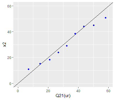
Figure 2: Q-Q plot for the distribution of $X_{2}\mid X_{1}>x_{1}$

The values of mean, standard deviation, $L$-covariance, $L$-correlation, $L$-coskewness and $L$-cokurtosis for the data were obtained as

$$E(X_{1})=17.62,\quad\text{Standard Deviation}(X_{1})=10.14$$

$$E(X_{2})=30.70,\quad\text{Standard Deviation}(X_{2})=14.54,$$

$$L\text{-covariance}=0.24,\quad L\text{-correlation}=0.53,$$

$$L\text{-coskewness}=0.30\text{ and }L\text{-cokurtosis}=0.25.$$

Since the variance of $X_{1}$ and $X_{2}$ are relatively larger than the respective mean, we conclude that the variables are likely to be overdispersive. The $L$-covariance is positive indicates that the variables move in the same direction but they have only a moderate relationship as indicated by the $L$-correlation of 0.53. The $L$-coskewness is positive is indicative of the fact that the variables undergo positive deviation at the same time. On the otherhand the $L$-cokurtosis being small shows that there are no extreme positive or negative deviations at the same time.

The second dataset was provided by Kim and Kvam, (2004), who tracked the failure times of 20 sample units from a three-component system. Since the present study considers the modelling of bivariate data, we have taken only the failure times of two components for the analysis as given in Table 2.

$X_{1}$	0.37	0.06	0.2	1.62	5.7	2.25	2.5	2.44	0.12	0.79	7.22	2.81	4.13	5.67	0.96	7.16	0.32	7.32	2.58	1.73
$X_{2}$	6.93	2.42	0.2	2.34	1.96	4.6	0.09	7.27	0.06	8.61	1.38	5.05	0.52	1.11	3.54	2.38	1.89	1.54	8.61	1.22

Table 2: Failure times two-components as reported in Kim and Kvam, (2004)

We calculate the estimates of the parameters as in the first case, to obtain

$$\hat{c}_{1}=13.0499,\ \hat{\alpha}_{1}=0.8856,\ \hat{\beta}_{1}=-0.1844$$

$$\hat{c}_{2}=5.9257,\ \hat{\alpha}_{2}=0.3555,\ \hat{\beta}_{2}=-0.6695\text{ and }\hat{\theta}=0.5492.$$

The Q-Q plots corresponding to $Q_{1}$ and $Q_{21}$ are exhibited in Figures 3 and 4 . Further, the K-S test values are $D_{1}=0.110$ and $D_{21}=0.133$ with respective $p$-values 0.310 and 0.277. Thus the data does not reject the bivariate complementary beta distribution with

$$q_{1}(u_{1}) =13.0499u_{1}^{0.8856}(1-u_{1})^{-0.1844}\;\text{ and }$$ (4.2)

$$q_{21}(u_{1},u_{2}) =(1+0.5492u_{1})5.9257u_{2}^{0.3555}(1-u_{2})^{-0.6695}.$$

Thus the second dataset also fits the model given in (2.1).

Using models (4.1) and (4.2) one can easily derive the desired characteristics of the distribution of $(X_{1},X_{2})$ based on the expressions in Section 3 and the probabilities of events of interest.

To examine the usefulness of the proposed model compared to some existing bivariate models, we proceed to fit the same data to the bivariate linear mean residual quantile model defined by Vineshkumar and Nair, (2019), given by

$$Q_{1}\left(u_{1}\right)=-\left(a_{1}+b_{1}\right)\log\left(1-u_{1}\right)-2b_{1}u_{1},0\leq u_{1}\leq 1,\,a_{1}>0,\,\left(a_{1}+b_{1}\right)>0$$ (4.3)

and

$$Q_{21}\left(u_{2}\mid u_{1}\right)=- \left(a_{2}+c+\left(b_{2}+d\right)u_{1}\right)\log\left(1-u_{2}\right)-2\left(c+du_{1}\right)u_{2},$$ (4.4)

$$0\leq u_{2}\leq 1,\,a_{2}+c>0,\,a_{2}>0,\,a_{2}+b_{2}\geq c+d.$$

The above bivariate model also do not have a closed form distribution functions. The method of $L$-moments are again employed for the estimation of parameters of the model, which are obtained as

$$\hat{a_{1}}=2.798,\,\hat{b_{1}}=0.159,\,\hat{a_{2}}=3.086,\,\hat{c}=0.086,\hat{b_{2}}=4.628,\,\text{ and }\hat{d}=-7.16,$$

Then the quantile functions (4.3) and (4.4) become

$$Q_{1}\left(u_{1}\right)=-\left(2.798+0.159\right)\log\left(1-u_{1}\right)-2*0.159*u_{1}$$ (4.5)

and

$$Q_{21}\left(u_{2}\mid u_{1}\right)=-\left(3.086+0.086+\left(4.628-7.16\right)u_{1}\right)\log\left(1-u_{2}\right)-2\left(0.086-7.16*u_{1}\right)u_{2}.$$ (4.6)

The $Q-Q$ plots corresponding to $Q_{1}$ and $Q_{21}$ in (4.5) and (4.6) are given in Figures 5 and 6 and the corresponding K-S test statistics values are $D_{1}=0.126$ and $D_{21}=0.322$ respectively. Thus the data does not reject the bivariate linear mean residual quantile function. Clearly, the K-S statistic value for the bivariate complementary beta model specified in (4.2) is small compared to the bivariate mean residual quantile model. This allow us to conclude that the proposed bivariate model is a better model for modelling the given bivariate data set.

Figure 3: Q-Q plot for the distribution of $X_{1}$

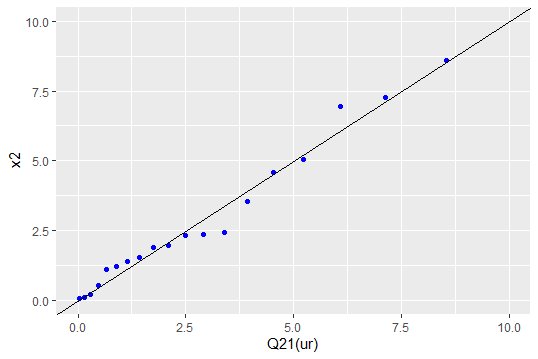
Figure 4: Q-Q plot for the distribution of $X_{2}\mid X_{1}>x_{1}$

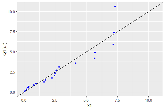
Figure 5: Q-Q plot for the distribution of $X_{1}$

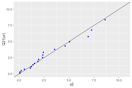
Figure 6: Q-Q plot for the distribution of $X_{2}\mid X_{1}>x_{1}$

5 Concluding Remarks

We have presented a flexible family of bivariate distribution based on a bivariate quantile function. The proposed family of bivariate distribution is characterized by the use of quantile functions. The model employs two primary functions: $Q_{1}\left(u_{1}\right)$, which represents the quantile function of the first variable $X_{1}$, and $Q_{21}\left(u_{1},u_{2}\right)$, which is the quantile function of the second variable $X_{2}$ given $Q_{1}(u_{1})$. This framework allows for the derivation of the marginal distribution $F_{1}\left(x_{1}\right)$ and the conditional distribution $F_{2}\left(x_{2}\mid x_{1}\right)$, leading to the joint distribution $F\left(x_{1},x_{2}\right)$. The model is highly flexible, allowing for the representation of a wide range of bivariate distributions by simply altering the parameter values. This versatility enables the modeling of various dependency structures and tail behaviors, making it applicable to numerous fields. The adaptability of the model to different bivariate distributions without requiring closed form expressions makes it suitable for a wide range of practical applications, providing a unified framework for bivariate analysis and makes the model more straightforward to implement and interpret. As quantile functions are less sensitive to outliers and extreme values compared to traditional distribution functions, enhances the model’s reliability and accuracy, particularly in heavy-tailed distributions and datasets with anomalies.

Generating random samples from the proposed bivariate distribution is efficient and straightforward. By simulating uniform random variables $u_{1}$ and $u_{2}$, we can easily obtain samples of $X_{1}$ and $X_{2}$ through the quantile functions $Q_{1}\left(u_{1}\right)$ and $Q_{21}\left(u_{1},u_{2}\right)$. This property is particularly beneficial in scenarios requiring large-scale simulations, where the computational efficiency and simplicity of the quantile-based approach significantly reduce the complexity. The use of quantile functions allows for the derivation of analytical expressions for marginal and conditional distributions, enhancing the model’s tractability. This facilitates the calculation of probabilities, moments, and other statistical measures, which are essential for practical applications and theoretical studies and simplifies the analysis and understanding of the dependence structure between $X_{1}$ and $X_{2}$.

Additionally, our model facilitates the use of $L$-moments for parameter estimation, offering several advantages. $L$-moments, which are linear combinations of order statistics, provide more robust estimates compared to traditional moments, especially in the presence of outliers or small sample sizes. One of the significant properties of $L$-moments is that if the mean of a distribution exists, then all higher-order $L$-moments also exist. This ensures that $L$-moments can be reliably used for a wide range of distributions. Their use in our quantile-based model enhances the estimation process, making it more robust and reliable. Several additional properties, characterizations and applications of the new distribution require separate consideration, in other areas require further examination.

Conflict of interest statement

On behalf of all the authors, the corresponding author states that there is no conflict of interest.

References

- Akhundov et al., (2004) Akhundov, I., Balakrishnan, N., and Nevzorov, V. (2004). New characterizations by properties of midrange and related statistics. Communications in Statistics, Theory and Methods, 33:3133–3143.
- Balakrishnan and Akhundov, (2003) Balakrishnan, N. and Akhundov, I. (2003). A characterization by linearity of the regression function based on order statistics. Statistics & Probability Letters, 63(4):435–440.
- Belzunce et al., (2007) Belzunce, F., Castaño, A., Olvera-Cervantes, A., and Suárez-Llorens, A. (2007). Quantile curves and dependence structure for bivariate distributions. Computational Statistics & Data Analysis, 51(10):5112–5129.
- Cai, (2010) Cai, Y. (2010). Multivariate quantile function models. Statistica Sinica, 20(2):481–496.
- Chen and Welsh, (2002) Chen, L.-A. and Welsh, A. (2002). Distribution-function-based bivariate quantiles. Journal of Multivariate Analysis, 83(1):208–231.
- Cuadras, (2002) Cuadras, C. M. (2002). On the covariance between functions. Journal of Multivariate Analysis, 81(1):19–27.
- David and Chaudhry, (2001) David, R. and Chaudhry, M. (2001). Coskewness and cokurtosis in futures markets. Journal of Empirical Finance, 8(1):55–81.
- Hosking, (1990) Hosking, J. R. M. (1990). L-moments: Analysis and estimation of distributions using linear combinations of order statistics. Journal of the Royal Statistical Society: Series B (Methodological), 52(1):105–124.
- Hosking and Wallis, (1997) Hosking, J. R. M. and Wallis, J. R. (1997). Regional Frequency Analysis: An Approach Based on L-Moments. Cambridge University Press, New York.
- Jones, (2002) Jones, M. (2002). The complementary beta distribution. Journal of Statistical Planning and Inference, 104(2):329–337.
- Jones, (2007) Jones, M. (2007). On a class of distributions defined by the relationship between their density and distribution functions. Communications in Statistics—Theory and Methods, 36(10):1835–1843.
- Jones, (2004) Jones, M. C. (2004). Families of distributions arising from distributions of order statistics. Test, 13:1–43.
- Kamps, (1991) Kamps, U. (1991). A general recurrence relation for moments of order statistics in a class of probability distributions and characterizations. Metrika, 38(1):215–225.
- Kim and Kvam, (2004) Kim, H. and Kvam, P. H. (2004). Reliability estimation based on system data with an unknown load share rule. Lifetime Data Analysis, 10:83–94.
- Lawless, (2011) Lawless, J. F. (2011). Statistical Models and Methods for Lifetime Data. John Wiley & Sons, New Jersey.
- Nair et al., (2013) Nair, N. U., Sankaran, P. G., and Balakrishnan, N. (2013). Quantile-based Reliability Analysis. Springer Science & Business Media, Boca Raton.
- Nair et al., (2012) Nair, N. U., Sankaran, P. G., and Vineshkumar, B. (2012). The Govindarajulu distribution: some properties and applications. Communications in Statistics-Theory and Methods, 41(24):4391–4406.
- Nair and Vineshkumar, (2022) Nair, N. U. and Vineshkumar, B. (2022). Modelling informetric data using quantile functions. Journal of Informetrics, 16(2):101266.
- Nair and Vineshkumar, (2023) Nair, N. U. and Vineshkumar, B. (2023). Properties of bivariate distributions represented by quantile functions. American Journal of Mathematical and Management Sciences, 42(1):1–12.
- Serfling and Xiao, (2007) Serfling, R. and Xiao, P. (2007). A contribution to multivariate L-moments: L-comoment matrices. Journal of Multivariate Analysis, 98(9):1765–1781.
- Vineshkumar and Nair, (2019) Vineshkumar, B. and Nair, N. U. (2019). Bivariate quantile functions and their applications to reliability modelling. Statistica, 79(1):3–21.
- Zsolt and Botond, (2021) Zsolt, N. B. and Botond, B. (2021). Co-skewness, co-kurtosis and their implications on asset pricing of cryptocurrencies. International Journal of Financial Markets and Derivatives, 8(1):65–78.