Numerical solution and errors analysis of iterative method for a nonlinear plate bending problem

Akakpo Amoussou Wilfried(a) and Houédanou Koffi Wilfrid(b)
Abstract.

This paper uses the HCT finite element method and mesh adaptation technology to solve the nonlinear plate bending problem and conducts error analysis on the iterative method, including a priori and a posteriori error estimates. Our investigation exploits Hermite finite elements such as BELL and HSIEH-CLOUGH-TOCHER (HCT) triangles for conforming finite element discretization. Then, the existence and uniqueness of the approximation solution are proven by using a variant of the Brezzi-Rappaz-Raviart theorem. We solve the approximation problem through a fixed-point strategy and an iterative algorithm, and study the convergence of the iterative algorithm, and provide the convergence conditions. An optimal a priori error estimation has been established. We construct a posteriori error indicators by distinguishing between discretization and linearization errors and prove their reliability and optimality. A numerical test is carried out and the results obtained confirm those established theoretically.

Mathematics Subject Classification [MSC]: 74S05,74S10,74S15, 74S20,74S25,74S30.
Key Words: Plate bending problem $\bullet$ Isotropic discretization $\bullet$ BELL and HCT Triangles $\bullet$ Iterative method $\bullet$ A priori error estimation $\bullet$ A posteriori error estimation.

1. Introduction

In this paper, we are interested in a numerical solution and a priori, and a-posteriori errors analysis of iterative method for a nonlinear plate bending problem. The numerical resolution is carried out using the HCT finite element method with mesh adaptation, allowing increased precision thanks to a local refinement based on error indicators. In indeed, the a posteriori error analysis initiated by Babuška [8] and improved by Verfürth [41] satisfies several objectives in the numerical resolution of PDEs, more precisely in the case of nonlinear PDEs. It makes it possible to globally control the discretization error of the problem posed by providing explicit bounds on the error between the numerical solution and the exact solution as soon as the approximate solution is known. This analysis can provide stopping criteria which guarantee overall error control and constitutes a basic tool for the construction of the adaptive mesh. In the context of nonlinear problems, Chaillou and Suri [12, 13] will initiate the construction of a posteriori error estimators by distinguishing between linearization and discretization errors. Then, this method will be developed within the framework of an iterative algorithm by L. El Alaoui, A. Ern [27]. Another iterative method is used by C. Bernardi, Jad Dakroub, Gihane Mansour and Tony Sayah [26] to provide us with a remarkable gain in terms of calculation time. This method is applied to the nonlinear Laplace problem. Furthermore, an error analysis for the bilaplacian problem is addressed in the literature by P.G. Ciarlet et al. and other authors in [17, 18, 19, 20, 21, 29, 9]. Different approximation approaches are discussed after a variational formulation. We note that the variational formulation of the bilaplacian equation is simple and its conforming discretization by finite elements requires finite elements of class $C^{1}$ which are rather expensive due to the high polynomial degree. To overcome this difficulty, they consider a mixed discretization, or a non-conforming approximation, each having its advantages and disadvantages. Verfürth used the three approaches with a posteriori residual error analysis in [41]. The nonlinear case of its problems are not too addressed. We study here a nonlinear case of the plate bending problem. Let $\Omega$ be a bounded open and connected of the ${\mathbb{R}}^{d}$ with lipschitzian boundary, $\Gamma=\partial\Omega$ the boundary of $\Omega$ , $d\in\{2,3\}$. We consider the plate bending nonlinear model:

(1.1) $$\begin{cases}\Delta^{2}u+\lambda|u|^{2p}u=f\text{ in }\Omega\\ u=0\text{ on }\Gamma\\ \dfrac{\partial u}{\partial n}=0\text{ on }\Gamma,\end{cases}$$

where $\lambda$ and $p$ are strictly positive real numbers, $f\in H^{-2}(\Omega)$ topological dual of $H^{2}_{0}(\Omega)$ and $n$ the unitary exterior normal at $\Gamma$. To our knowledge, there is no a posteriori error estimation result of the problem (1.1)(\ref{p}) where a conforming finite element method is used. Here, we develop such a posteriori error analysis using isotropic (or regular) mesh. One of the main differences between our paper and the reference [26] is that the unknown solution of the problem (1.1)(\ref{p}) has regularity $H_{0}^{2}(\Omega)$. This requires more regular finite elements. The standard Lagrange finite elements used in [26] are no longer appropriate. Our investigation uses Hermite finite elements, namely BELL and HSIEH-CLOUGH-TOCHER (HCT) Triangles [4, 5, 6], which assure inclusion of our space approximation $V_{h}$ in $H_{0}^{2}(\Omega)$ [see 3.21 ].

The problem (1.1)(\ref{p}) may arise in various contexts of mathematical physics, including solid mechanics, theory of elastic plates, differential geometry. By examining its components, it could model a physical system where an unknown $u$ is subject to forces described by the function $f$, and where deformations are subject to power-type non linearities and specific boundary conditions on the domain boundary. Thus, the equation (1.1)1(\ref{p})_{1} could be applied to various scenarios where these conditions are satisfied, such as elastic plate deformations, nonlinear wave propagation phenomena. Furthermore, one may notice a similarity between this equation (1.1)1(\ref{p})_{1}, which are often used to describe phenomena such as liquid-liquid or solid-solid phase separation in metal alloys, grain growth in polycrystalline materials [3, 15, 16]. We noted that, the equation (1.1)1(\ref{p})_{1} is particularly the Cahn-Hilliard equation in two dimension [40].

Plan of the paper. The contents of this paper have been organized in the following manner. For the nonlinear problem (1.1), we introduce a variational formulation (2.5)(\ref{fv}) and prove the existence and uniqueness of the exact solution in section 2. In section 3, we develop a conforming discretization of the variational problem (1.1) using Hermite finite elements and prove the existence and uniqueness of an approximate solution according to the Brezzi-Rappaz-Raviart theorem (cf. Theorem 3.1) for the approximation of nonlinear problems. Some technical results have been developed in section 3.2, with fixed point strategy. Afterwards, in section 3.4, we use an iterative algorithm (Banach-fixed point) to make an appropriate linearization (3.23) of the approximate problem (3.1), and in the section 3.5 we study the convergence of this algorithm towards the solution of the discrete problem. A priori error analysis has been deveoped in section 4.1. An important step is to derive a posteriori error estimates by distinguishing between linearization and discretization errors. In section 4.2, the a posteriori error estimates are derived. We define the error indicators (see Definition 4.1), and the upper error bound has been established in subsection 4.2.1 while the lower error bound is proved in subsection 4.2.2. Section 5 is devoted to numerical results. Its subsection 5.1 presents the numerical solution after convergence, while subsection 5.2 shows the evolution of the error at each mesh size. Subsection 5.3 shows us the behavior of local error indicators with errors. An adaptation of meshes according to these errors indicators is presented in the subsection 5.4. In the section 5.5, we analyze the performance of the developed method through numerical results, highlighting its accuracy, robustness and relevance for solving complex problems. We offer our conclusion and the further works in section 6.

2. Weak formulation

We describe in this section the nonlinear problem (1.1) together with its variational formulation and we proof existence and uniqueness of exact solution of the nonlinear problem. First of all, we recall the main notion and results which we use later on. If $\mathcal{O}$ is a bounded open domain of $\mathbb{R}^{d}$ , we denote by $L^{p}(\mathcal{O})$ the space of measurable functions summable with power $p$. For $v\in L^{p}(\mathcal{O})$ , the norm is defined by,

(2.1) $$\|v\|_{L^{p}(\mathcal{O})}=\left[\int_{\mathcal{O}}|v(x)|^{p}dx\right]^{\frac{1}{p}}.$$

Now, we introduce some Sobolev spaces and norms [11]. Let $m\in\mathbb{N}$ and $\ d\in\mathbb{N}^{*}$ where $\mathbb{N}$ is the set of natural numbers, and $\mathbb{N}^{*}$ is the set of nonzero natural numbers, $1\leqslant p<\infty$, a real number. The Sobolev space $W^{m,p}(\mathcal{O})$ is defines by:

$$W^{m,p}(\mathcal{O}):=\left\{v\in{L^{p}(\mathcal{O})}:D^{\alpha}v\in{L^{p}(\mathcal{O})}\ \forall\alpha=(\alpha_{1},\alpha_{2},\ldots,\alpha_{d})\in\mathbb{N}^{d}:\sum_{i=1}^{d}\alpha_{i}=|\alpha|\leqslant m\right\},$$

with the norm:

(2.2) $$\|v\|_{W^{m,p}(\mathcal{O})}:=\left[\sum_{|\alpha|\leqslant m}\|D^{\alpha}v\|^{p}_{L^{p}(\mathcal{O})}\right]^{\frac{1}{p}},\ 1\leqslant p<\infty\ \forall v\in W^{m,p}(\mathcal{O}).$$

The Sobolev space $H^{m}(\mathcal{O})=W^{m,2}(\mathcal{O})$ is defined in the usual way with the usual norm $\parallel\cdot\parallel_{m,\mathcal{O}}$ and semi-norm $|\cdot|_{m,\mathcal{O}}$. In particular, $H^{0}(\mathcal{O})=L^{2}(\mathcal{O})$ and we write $\parallel\cdot\parallel_{\mathcal{O}}$ for $\parallel\cdot\parallel_{0,\mathcal{O}}$. Similarly we denote by $(\cdot,\cdot)_{\mathcal{O}}$ the $L^{2}(\mathcal{O})$ inner product. For shortness if $\mathcal{O}$ is equal to $\Omega$, we will drop the index $\Omega$. The space $H_{0}^{m}(\mathcal{O})$ denotes the closure of $\mathcal{C}_{c}^{\infty}(\mathcal{O})$ in $H^{m}(\mathcal{O})$ and $H^{-m}(\mathcal{O})$ is topological dual space of $H_{0}^{m}(\mathcal{O})$, equipped with the norm:

(2.3) $$\|z\|_{-m,\mathcal{O}}=\sup_{{u\in H_{0}^{m}(\mathcal{O})}-\{0\}}\dfrac{|\langle z,u\rangle|}{\|u\|_{m,\mathcal{O}}}\quad\forall z\in H^{-m}(\mathcal{O}).$$

If the open domain $\mathcal{O}$ is bounded, connected and has a lipschitzian boundary, then for $m=2$, the map $u\mapsto\|\Delta u\|_{L^{2}(\mathcal{O})}$ is a norm equivalent to $|\cdot|_{2,\mathcal{O}}$ on $H_{0}^{2}(\mathcal{O})$ [33]. Moreover, for all integer $m\geqslant 0$ and for all $p\in[1,+\infty[$, we have the following inclusions with continuous injections [1, Chapter 3]: $W^{m,p}(\mathcal{O})\hookrightarrow L^{p^{*}}({\mathcal{O}})\text{ if }m<\tfrac{d}{p}$, $W^{m,p}(\mathcal{O})\hookrightarrow L^{q}({\mathcal{O}}),q\geq 1\text{ if }m=\tfrac{d}{p}$ and $W^{m,p}(\mathcal{O})\hookrightarrow\mathcal{C}^{0}(\bar{\mathcal{O}})\text{ if }m>\tfrac{d}{p},\mbox{ with }p^{*}=\tfrac{pd}{d-mp}$.
Recurrent notation. In the sequel, we denote by $C$, $C^{\prime}$, $c_{1}$, $c_{2}$, $c_{1}^{\prime}$, $\ldots$, generic constants that can vary from line to line but are always independent of all discretization parameters.
We have the following lemma:

Lemma 2.1.

(cf. [11]) For all $p\in\ ]1,+\infty[$, there exists a strictly positive real constant $C_{p}$ such that :

(2.4) $$\sup_{x\in\bar{\mathcal{O}}}|v(x)|\leqslant C_{p}\|v\|_{W^{m,p}(\mathcal{O})},\forall v\in W^{m,p}(\mathcal{O}),\mbox{ if }m>\frac{d}{p}.$$

The nonlinear model problem (1.1) admits the equivalent variational formulation: find $u\in V:=H_{0}^{2}(\Omega)$ such that,

(2.5) $$\int_{\Omega}\Delta u(x)\Delta v(x)dx+\lambda\int_{\Omega}|u|^{2p}u(x)v(x)dx=\langle f,v\rangle_{H^{-2}(\Omega)},\forall v\in V.$$

Our problem being nonlinear, the Lax-Milgram theorem cannot be used to show the existence and uniqueness of solution. We will therefore resort to the minimization results [30].

Theorem 2.1.

(ref. [30]) Let $H$ be a reflexive Banach space, $K$ a closed convex of $H$ and $J:K\to\mathbb{R}$ a convex function lower semi-continuous (abbreviated s-c-i) if $K$ is unbounded, suppose that for any sequence $(u_{n})_{n}$ of $K$ such that $\|u_{n}\|\to+\infty$, when $n\to+\infty$, we have $J(u_{n})\to+\infty$. Then $J$ reaches its minimum on $K$ :

(2.6) $$\exists u\in K,J(u)=\inf_{v\in K}J(v)=\min_{v\in K}J(v).$$

Moreover if $J$ is strictly convex, $u$ is unique.

We introduce the following definition:

Definition 2.1.

The functional (a map from a vector space of functions to its scalar body) energy associated with the nonlinear model problem (1.1)(\ref{p}) is defined by:

(2.7) $$J(u)=\dfrac{1}{2}\int_{\Omega}|\Delta u|^{2}dx+\dfrac{\lambda}{2p+2}\int_{\Omega}|u|^{2p}[u(x)]^{2}dx-\langle f,u\rangle_{H^{-2}(\Omega)},\forall u\in H_{0}^{2}(\Omega).$$
Remark 2.1.

(Differential of $J$) Since $\mathcal{C}_{c}^{\infty}(\Omega)$ is dense in $H^{2}_{0}(\Omega)$ for the norm of $H^{2}(\Omega)$, then

$$J^{\prime}(u)=0\text{ in }[\mathcal{C}_{c}^{\infty}(\Omega)]^{\prime}\mbox{ equivalently to }\Delta^{2}(u)+\lambda|u|^{2p}u-f=0\text{ in }[\mathcal{C}_{c}^{\infty}(\Omega)]^{\prime}.$$

Now, we can proof the existence and uniqueness of exact solution of the nonlinear problem (1.1). We have the following result:

Theorem 2.2.

The nonlinear plate bending problem (1.1)(\ref{p}) admits a unique solution $u\in H^{2}_{0}(\Omega).$

Proof.

For the proof of Theorem 2.2, we use Theorem 2.1 by verifying each assumption. The closed space $V=H^{2}_{0}(\Omega)$ then $V$ is convex. Let us show the energy functional $J$ defines by (2.7) is convex. Let’s pose

(2.8) $\displaystyle g_{1}(u)$ $\displaystyle=$ $\displaystyle\displaystyle\int_{\Omega}|\Delta u(x)|^{2}dx,$
(2.9) $\displaystyle g_{2}(u)$ $\displaystyle=$ $\displaystyle\displaystyle\int_{\Omega}|u(x)|^{2p}[u(x)]^{2}dx,$
(2.10) $\displaystyle g_{3}(u)$ $\displaystyle=$ $\displaystyle\langle f,v\rangle_{H^{-2}(\Omega)\times H_{0}^{2}(\Omega)}.$

The function $g_{3}$ is a linear form. Therefore it is convex and $g_{2}$ is strictly convex, because the function $x\mapsto|x|^{2p+2}$ is strictly convex. Let $u,v\in V$ and $t\in[0,1]$ we have: $(1-t)u+tv\in H_{0}^{2}(\Omega)$ and

$\displaystyle g_{1}((1-t)u+tv)$ $\displaystyle=$ $\displaystyle\displaystyle\int_{\Omega}|\Delta((1-t)u+tv)|^{2}dx,$
$\displaystyle\leqslant$ $\displaystyle\displaystyle\int_{\Omega}\left[(1-t)|\Delta u|+t|\Delta v|\right]^{2}dx.$

Using the Cauchy-Schwarz inequalities, we obtain $g_{1}((1-t)u+tv)\leqslant(1-t)g_{1}(u)+tg_{1}(v)$ and $g_{1}$ is convex. We deduce from everything that $J$ is strictly convex as the sum of convex and strictly convex functions. Let us show that $J$ is coercive. Since $\displaystyle\int_{\Omega}fudx\leq\left|\displaystyle\int_{\Omega}fudx\right|\leqslant\|f\|_{-2,\Omega}\|u\|_{2,\Omega}\leqslant\frac{s}{2}\|u\|^{2}_{2,\Omega}+\frac{1}{2s}\|f\|^{2}_{-2,\Omega},$(Young inequality) then $-\displaystyle\int_{\Omega}fudx\geqslant-\frac{s}{2}\|u\|^{2}_{2,\Omega}-\frac{1}{2s}\|f\|^{2}_{-2,\Omega}.$ We deduce that,

$$\begin{array}[]{ccc}J(u)&\geqslant&\min\left(\dfrac{1}{4},\dfrac{\lambda}{2p+2}\right)\left[\|u\|^{2}_{2,\Omega}+\|u\|^{2p+2}_{L^{2p+2}(\Omega)}\right]-\|f\|^{2}_{-2,\Omega}\text{ for }s=\frac{1}{2}.\end{array}$$

Hence the coercivity. Furthermore, the energy functional being differentiable for everything $v\in H_{0}^{2}(\Omega)$, then it is continuous on $H_{0}^{2}(\Omega)$ and consequently s-c-i on $H_{0}^{2}(\Omega)$. We conclude, according to Theorem 2.1, the nonlinear problem (1.1)(\ref{p}) admits a unique solution in $H_{0}^{2}(\Omega)$. ∎

3. Finite element discretization

3.1. Discrete problem

Let $h>0$ be a real parameter. The objective here is to replace the space $V$ by a vector subspace of finite dimension $V_{h}$ called the space of approximation. This is the continuous Galerkin method. For construction of $H_{0}^{2}(\Omega)$-conforming approximation $V_{h}$ [cf. (3.21) below], we use the BELL and HSIEH-CLOUGH-TOCHER elements [35] that we present in section 3.3. The discrete problem (3.1) associated to the plate bending nonlinear problem (1.1)(\ref{p}) is as follows: find $u_{h}\in V_{h}$ such that,

(3.1) $$\int_{\Omega}\Delta u_{h}(x)\Delta v_{h}(x)dx+\int_{\Omega}\lambda|u_{h}(x)|^{2p}u_{h}(x)v_{h}(x)dx=\langle f,v_{h}\rangle\ \forall v_{h}\in V_{h}.$$

In order to prove the existence and uniqueness of a solution to problem (3.1), we use the Brezzi-Rappaz-Raviart theorem (cf. [10]). This theorem will also allow us to control the corresponding a priori error estimator. Before stating the theorem, we specify certain hypotheses. Let $X$ and $Y$ be two Banach spaces. We introduce a class $C^{1}$ map, $G:X\to Y$ and continuous linear map $S\in\mathcal{L}(Y,X)$. We put for all $u\in X,$

(3.2) $$F(u)=u-S\circ G(u).$$

We consider a finite element approximation of a solution $u\in X$ of the problem (3.3) below:

(3.3) $$F(u)=0\text{ i.e. }u-S\circ G(u)=0.$$

For $h>0$ a real, we give ourselves a finite-dimensional vector subspace $X_{h}$ of $X$ and an associated operator $S_{h}\in\mathcal{L}(Y,X_{h})$ . The approximate problem of (3.3)(\ref{F}) consists of finding $u_{h}\in X_{h}$ solution to the equation :

(3.4) $$F_{h}(u_{h})=0,\mbox{ where }F_{h}(u_{h})=u_{h}-S_{h}\circ G(u_{h}).$$

Then, we have the following theorem (cf. [10]):

Theorem 3.1.

[10] We assume that $G$ is a map of class $C^{1}$ from $X$ to $Y$ such that $G^{\prime}$ is lipschitz continuous on the bounded subsets of $X$, i.e. there exists a function $L:\mathbb{R}_{+}\times\mathbb{R}_{+}\to\mathbb{R}_{+}$ monotonically increasing with respect to each variable such that for all $u,w\in X,\|G^{\prime}(u)-G^{\prime}(w)\|_{\mathcal{L}(X,Y)}\leqslant L(\|u\|_{X},\|w\|_{X})\|u-w\|_{X}$, $S\circ G^{\prime}(u)\in\mathcal{L}(X)$ is compact and $F^{\prime}(u)$ is an isomorphism of $X$. Furthermore, we assume that for all $v\in X$,

(3.5) $$\lim\limits_{h\to 0}\|v-\Pi_{h}v\|_{X}=0,$$

for a certain linear operator $\Pi_{h}\in\mathcal{L}(X,X_{h})$ and

(3.6) $$\lim\limits_{h\to 0}\|S_{h}-S\|_{\mathcal{L}(Y,X)}=0.$$

Then, there exists $h_{0}>0$ and an open neighborhood $\mathcal{O}$ of the origin in $X$ such that, for each $h\leqslant h_{0},$ the problem (3.3)(\ref{F}) admits a unique solution $u_{h}$ satisfying $u_{h}-u\in\mathcal{O}$. Furthermore, we have, for a certain constant $M>0$ independent of $h$, the estimate:

(3.7) $$\|u_{h}-u\|_{X}\leqslant M(\|u-\Pi_{h}u\|_{X}+\|(S_{h}-S)\circ G(u)\|_{X}).$$

In this paper, we apply the theorem 3.1 to problem (3.1)(\ref{pd}), namely (3.4). To do this, we need some technical results.

3.2. Fixed-point strategy and Some technical results

3.2.1. Fixed-point strategy

Let $X=H^{2}_{0}(\Omega)$ and $Y=H^{-2}(\Omega)$. For the application $G:X\to Y$ and the map linear continuous $S\in\mathcal{L}(Y,X)$ of Theorem 3.1, we define:

(3.8) $\displaystyle G(w)=f-\lambda|w|^{2p}w,\forall w\in X$

and

(3.9) S:YXφS(φ),\begin{tabular}[]{cccc}$S:$&$Y$&$\to$&$X$\\ &$\varphi$&$\mapsto$&$S(\varphi)$\end{tabular},

such that if $S(\varphi)=w$, then $w$ is the solution to the problem:

(3.10) $$\begin{cases}\Delta^{2}w=\varphi\text{ in }\Omega\\ w=\dfrac{\partial w}{\partial n}=0\text{ on }\Gamma.\end{cases}$$

We noted that, the problem (3.10)(\ref{p'}) admits a unique $w\in H_{0}^{2}(\Omega)$ solution to the equivalent variational problem:

(3.11) $$\displaystyle\int_{\Omega}\Delta w(x)\Delta v(x)dx=\int_{\Omega}\varphi(x)v(x)dx,\forall v\in H_{0}^{2}(\Omega),$$

and $S\in\mathcal{L}(Y,X)$ satisfies the inequality:

(3.12) $$\parallel S(\varphi)\parallel_{2,\Omega}\leq\parallel\varphi\parallel_{-2,\Omega}.\forall\varphi\in H^{-2}(\Omega).$$

Let introduce the following proposition:

Proposition 3.1.

Let $G$ define by (3.8)(\ref{g}) and $S$ define by (3.9)(\ref{s}). Then, the problems (1.1)(\ref{p}) and (3.3)(\ref{F}) are equivalent.

Proof.

Assume that $u\in X$ is solution of (1.1)(\ref{p}). Then, $u$ check $\lambda|u|^{2p}u=-\Delta^{2}u+f$. From the definition of $S$ and $G$, that is, (3.8)(\ref{g}) and (3.9)(\ref{s}), we obtain $f-G(u)=0.$ As $f-G(u)\in Y=H^{-2}(\Omega)$ and $S$ is linear, composing the above equality by $S$, we deduce $S[f-G(u)]=0$ namely, $u-S\circ G(u)=0$, and we have $F(u)=0$, since $S(f)=u$. Reciprocally, assume that $u-S\circ G(u)=0$. From the definition of $S$ we have $S\circ G(u)=u$, and therefore by (3.9)(\ref{s}), $\Delta^{2}u=G(u)\text{ in }\Omega\mbox{ with }u=0=\dfrac{\partial u}{\partial n}\text{ on }\Gamma.$ The definition of $G$, i.e. (3.8)(\ref{g}) conclude the result.

3.2.2. Some technical results

Proposition 3.2.

(Technical inequality) Let $a,b$ and $s$ be three strictly positive real numbers. Then, we have the following inequality:

(3.13) $$|a^{s}-b^{s}|\leqslant s|a-b|\left[a^{s-1}+b^{s-1}\right].$$
Proof.

Let $a,b$ and $s$ be three elements of $]0,+\infty[$. Now, we consider the function $\varphi\in\mathcal{C}^{1}([a,b],\mathbb{R})$, $\varphi:[a,b]\rightarrow\mathbb{R}$ define by $\varphi(x)=x^{s}$ . Then, there exists $c\in]a,b[$ constant such that $\varphi(a)-\varphi(b)=(a-b)\varphi^{\prime}(c)$. But $\varphi^{\prime}(x)=sx^{s-1}$, so we have $|a^{s}-b^{s}|=s|a-b||c^{s-1}|\leqslant s|a-b|\displaystyle\sup_{t\in[a,b]}|t^{s-1}|$. Hence $|a^{s}-b^{s}|\leqslant s|a-b|\left[a^{s-1}+b^{s-1}\right].$


To be able to verify the assume of Theorem 3.1, we need to prove some important properties satisfy by $G$ define in (3.8)(\ref{g}) and $S$ define in (3.9)(\ref{s}) that will be used later. The first lemma proves that the differential $G^{\prime}:H_{0}^{2}(\Omega)\to\mathcal{L}(H_{0}^{2}(\Omega),H^{-2}(\Omega))$ is Lipschitz continuous on the bounded subsets of $H_{0}^{2}(\Omega)$.

Lemma 3.1.

Let $G$ be the application define by (3.8). Then,
$G^{\prime}:H_{0}^{2}(\Omega)\to\mathcal{L}(H_{0}^{2}(\Omega),H^{-2}(\Omega))$ is Lipschitz continuous on the bounded subsets of $H_{0}^{2}(\Omega)$, where $G^{\prime}$ is the differential of $G$.

Proof.

We can recall that $X:=H_{0}^{2}(\Omega)$ and $Y=H^{-2}(\Omega)$. Now, let $u\in X$. It is well known that $G(u)=f-\lambda|u|^{2p}u$ . The application $G$ is differentiable and its differential at $u\in X$ is given for $v\in X$ by: $G^{\prime}(u)\cdot v=-\lambda(2pvu^{2p-1}u+u^{2p}v)$, namely $G^{\prime}(u)\cdot v=-\lambda(2p+1)|u|^{2p}v\ \forall\ v\in X.$ To show that $G^{\prime}$ is Lipschitz continuous on the bounded subsets of $H_{0}^{2}(\Omega)$, we will look for $L\in\mathbb{R}_{+}$ such that for all $(u,w)\in X^{2}$ we have $\|G^{\prime}(u)-G^{\prime}(w)\|_{\mathcal{L}(X,Y)}\leqslant L\|u-w\|_{X}.$ Let’s remember that:

(3.14) $$\|G^{\prime}(u)-G^{\prime}(w)\|_{\mathcal{L}(X,Y)}=\sup_{v\in X^{*}}\dfrac{\|(G^{\prime}(u)-G^{\prime}(w))\cdot v\|_{Y}}{\|v\|_{X}},$$

and

(3.15) $$\|(G^{\prime}(u)-G^{\prime}(w))\cdot v\|_{Y}=\sup_{z\in X^{*}}\dfrac{|\langle(G^{\prime}(u)-G^{\prime}(w))\cdot v),z\rangle|}{\|z\|_{X}}.$$

$\begin{array}[]{ccc}(G^{\prime}(u)-G^{\prime}(w))\cdot v&=&G^{\prime}(u)\cdot v-G^{\prime}(w)\cdot v\\ \\ &=&-\lambda(2p+1)|u|^{2p}v+\lambda(2p+1)|w|^{2p}v\\ \\ &=&-\lambda(2p+1)(|u|^{2p}-|w|^{2p})\cdot v\\ \\ \langle(G^{\prime}(u)-G^{\prime}(w))\cdot v,z\rangle&=&\displaystyle\int_{\Omega}\big{(}-\lambda(2p+1)(|u|^{2p}-|w|^{2p})\cdot v\big{)}zdx\\ \\ &=&-\lambda(2p+1)\displaystyle\int_{\Omega}[(|u|^{2p}-|w|^{2p})\cdot v]zdx.\end{array}$
Let’s calculate $\displaystyle\int_{\Omega}[(|u|^{2p}-|w|^{2p})\cdot v]zdx$. According to inequality 3.13 of Proposition 3.2 and the Lemma 2.1, we have $|u|^{2p}-|w|^{2p}\leqslant||u|^{2p}-|w|^{2p}|$, namely
$|u|^{2p}-|w|^{2p}\leqslant 2p|u-w|(|u|^{2p-1}+|w|^{2p-1}).$ Now,

$\displaystyle\displaystyle\int_{\Omega}[(|u|^{2p}-|w|^{2p})\cdot v]zdx$ $\displaystyle\leqslant$ $\displaystyle 2p\int_{\Omega}|u-w|(|u|^{2p-1}+|w|^{2p-1})|v||z|dx,$
$\displaystyle\leqslant$ $\displaystyle 2p\left[c_{1}|u-w|_{2,\Omega}(2c_{2}^{(2p-1)}(\|u\|^{2p-1}_{2,\Omega}+\|w\|^{2p-1}_{2,\Omega}))c_{3}|v|_{2,\Omega}c_{4}|z|_{2,\Omega}\right],$

which implies that,

$$\int_{\Omega}[(|u|^{2p}-|w|^{2p})\cdot v]zdx\leqslant 4pc_{1}c^{(2p-1)}_{2}c_{3}c_{4}(\|u\|^{2p-1}_{2,\Omega}+\|w\|^{2p-1}_{2,\Omega})|u-w|_{2,\Omega}|z|_{2,\Omega}|v|_{2,\Omega}.$$

Either,

$$\langle G^{\prime}(u)-G^{\prime}(w))\cdot v),z\rangle\leqslant-4\lambda pc_{1}c^{(2p-1)}_{2}c_{3}c_{4}(\|u\|^{2p-1}_{2,\Omega}+\|w\|^{2p-1}_{2,\Omega})|u-w|_{2,\Omega}|z|_{2,\Omega}|v|_{2,\Omega},$$

therefore,

$$\dfrac{|\langle(G^{\prime}(u)-G^{\prime}(w))\cdot v,z\rangle|}{\|z\|_{X}}\leqslant 4\lambda pc_{1}c^{(2p-1)}_{2}c_{3}c_{4}(\|u\|^{2p-1}_{2,\Omega}+\|w\|^{2p-1}_{2,\Omega})|u-w|_{2,\Omega}|v|_{2,\Omega}\ \forall z\in X^{*}.$$

By setting $L=L(\|u\|_{2,\Omega},\|w\|_{2,\Omega})=4\lambda pc_{1}c^{(2p-1)}_{2}c_{3}c_{4}(\|u\|^{2p-1}_{2,\Omega}+\|w\|^{2p-1}_{2,\Omega})\in\mathbb{R}_{+}$ we can arrive at

$$\sup_{z\in X^{*}}\dfrac{|<(G^{\prime}(u)-G^{\prime}(w))\cdot v,z>|}{\|z\|_{X}}\leqslant L|u-w|_{2,\Omega}|v|_{2,\Omega},$$

i.e

$$\|(G^{\prime}(u)-G^{\prime}(w))\cdot v\|_{Y}\leqslant L|u-w|_{2,\Omega}|v|_{2,\Omega},$$

which implies that

$$\dfrac{\|(G^{\prime}(u)-G^{\prime}(w))\cdot v\|_{Y}}{\|v\|_{X}}\leqslant L|u-w|_{2,\Omega}.$$

Hence,

$$\sup_{v\in X^{*}}\dfrac{\|(G^{\prime}(u)-G^{\prime}(w))\cdot v\|_{Y}}{\|v\|_{X}}\leqslant L|u-w|_{2,\Omega}.$$

Thus, we have $\|G^{\prime}(u)-G^{\prime}(w)\|_{\mathcal{L}(X,Y)}\leqslant L|u-w|_{2,\Omega}.$ Since $L$ is bounded with respect to each variable $u$ and $w$ on the bounded subsets of $H_{0}^{2}(\Omega)$, then $G^{\prime}$ satisfies the uniform Lipschitz condition. This completes the proof. ∎

The second property prove that the map $S\circ G^{\prime}(u):X\to X$ is linear continuous and compact on $X$, where $u\in X$.

Lemma 3.2.

Let $u\in X=H_{0}^{2}(\Omega)$. The map $S\circ G^{\prime}(u):X\to X$ is linear continuous and compact on $X$, where $G$ and $S$ are defined by (3.8) and (3.9) respectively.

Proof.

$S$ and $G^{\prime}(u)$ are two continuous linear maps on $Y$ and $X$ respectively. Then their composite is a continuous linear map. Let us show that $S\circ G^{\prime}(u)$ is compact. Let $B_{X}$ be the unit ball of $X$. Then, we proof that $G^{\prime}(u)(B_{X})$ is relatively compact. $B_{X}$ being bounded and $G^{\prime}(u)$ continuous, then $G^{\prime}(u)(B_{X})$ is a bounded part of $Y$. Let us show that $G^{\prime}(u)(B_{X})=\mathcal{H}$ is uniformly equicontinuous.
For $\varepsilon>0$, let’s search $\alpha>0$ such that $\forall(w_{1},w_{2})\in X^{2}$, and $v\in B_{X}$ we have, $\|w_{1}-w_{2}\|_{X}\leqslant\alpha$ implies $|\langle G^{\prime}(u)\cdot v,w_{1}\rangle-\langle G^{\prime}(u)\cdot v,w_{2}\rangle|\leqslant\varepsilon.$ We have

$\displaystyle|\langle G^{\prime}(u)\cdot v,w_{1}\rangle-\langle G^{\prime}(u)\cdot v,w_{2}\rangle|$ $\displaystyle=$ $\displaystyle|\langle G^{\prime}(u)\cdot v,w_{1}-w_{2}\rangle|.$

It is well known that, $G^{\prime}(u)\cdot v=-\lambda(2p+1)|u|^{2p}v$. Hence,

$\displaystyle|\langle G^{\prime}(u)\cdot v,w_{1}-w_{2}\rangle|$ $\displaystyle\leqslant$ $\displaystyle\lambda(2p+1)|\int_{\Omega}|u|^{2p}v(w_{1}-w_{2})dx|,$
$\displaystyle\leqslant$ $\displaystyle\lambda(2p+1)\int_{\Omega}||u|^{2p}v||w_{1}-w_{2}|dx,$
$\displaystyle\leqslant$ $\displaystyle\lambda\mbox{mes}(\Omega)(2p+1)c_{1}c_{2}\|u\|_{L^{2p}(\Omega)}^{2p}|v|_{2,\Omega}|w_{1}-w_{2}|_{2,\Omega}.$

By setting $k^{\prime}=\lambda mes(\Omega)(2p+1)c_{1}c_{2}\|u\|_{L^{2p}(\Omega)}^{2p}>0$ we obtain,

$$|\langle G^{\prime}(u)\cdot v,w_{1}-w_{2}\rangle|\leqslant k^{\prime}\|v\|_{X}|w_{1}-w_{2}|_{2,\Omega},$$

which implies, $|\langle G^{\prime}(u)\cdot v,w_{1}-w_{2}\rangle|\leqslant k^{\prime}|w_{1}-w_{2}|_{2,\Omega}$, since $v\in B_{X}$, i.e. $\parallel v\parallel_{X}\leq 1$. So that $|\langle G^{\prime}(u)\cdot v,w_{1}\rangle-\langle G^{\prime}(u)\cdot v,w_{2}\rangle|\leqslant\varepsilon$, it suffices that $k^{\prime}|w_{1}-w_{2}|_{2,\Omega}\leqslant\varepsilon$, namely,
$|w_{1}-w_{2}|_{2,\Omega}\leqslant\dfrac{\varepsilon}{k^{\prime}}$, and thus, we take $\alpha=\dfrac{\varepsilon}{k^{\prime}}>0$. We deduce that $G^{\prime}(u)(B_{X})$ is uniformly equicontinuous. $G^{\prime}(u)(B_{X})$ is bounded and uniformly equicontinuous, according to Ascoli’s theorem [28], $G^{\prime}(u)(B_{X})$ is relatively compact. Therefore $G^{\prime}(u)$ is compact. Finally, $S$ being continuous and $G^{\prime}(u)$ compact, then $S\circ G^{\prime}(u)$ is compact and the proof is complete. ∎

The third property proves that the application $F^{\prime}(u):X\rightarrow X$ is an isomorphism, where $F$ is defined by (3.2) and $u\in X$.

Lemma 3.3.

Let $u\in X$. Assuming that $G$ is defined by (3.8) and $S$ defined by (3.9)(\ref{s}), then the map $F^{\prime}(u):X\to X$ is an isomorphism of $X$, where $F$ is defined by (3.2)(\ref{F'}) and $X=H_{0}^{2}(\Omega)$.

Proof.

By assumption, we have $F(u)=u-S\circ G(u)$ and the function $F$ is differentiable as the sum of a differentiable function and the composite of two differentiable functions. Since $S\in\mathcal{L}(Y,X)$, we have $F^{\prime}(u)=I-S^{\prime}[G(u)]\circ G^{\prime}(u)$, that is $F^{\prime}(u)=I-S\circ G^{\prime}(u)$, which implies $F^{\prime}(u)\cdot v=v-S\circ G^{\prime}(u)\cdot v$. According to Lemma 3.2  $S\circ G^{\prime}(u)$ is a compact operator, and from the Fredholm Alternative [11], $F^{\prime}(u)$ is an isomorphism on $V$ if the equation $[I-S\circ G^{\prime}(u)](w)=0$ admits a unique solution $w=0$. The condition $[I-S\circ G^{\prime}(u)](w)=0$ equivalent to $[S\circ G^{\prime}(u)](w)=w$. By definition of $S$, $S[G^{\prime}(u)\cdot w]=w$ implies that $w$ is the solution to the problem:

(3.16) $$\begin{cases}\Delta^{2}w=G^{\prime}(u)\cdot w\text{ in }\Omega\\ w=0=\dfrac{\partial w}{\partial n}\text{ on }\Gamma.\end{cases}$$

It is well known that $G^{\prime}(u)\cdot w=-\lambda(2p+1)|u|^{2p}w$ and so, we obtain auxiliary system,

(3.17) $$\begin{cases}\Delta^{2}w=-\lambda(2p+1)|u|^{2p}w\text{ in }\Omega\\ w=\dfrac{\partial w}{\partial n}=0\text{ on }\Gamma,\end{cases}$$

which implies,

(3.18) $$\begin{cases}\Delta^{2}w+\lambda(2p+1)|u|^{2p}w=0\text{ in }\Omega\\ w=\dfrac{\partial w}{\partial n}=0\text{ on }\Gamma,\end{cases}\text{ with }\lambda>0.$$

According to Proposition 3.1, we deduce that $[I-S\circ G^{\prime}(u)](w)=0$ is equivalent to (3.18)(\ref{po}). Consequently, $[I-S\circ G^{\prime}(u)](w)=0$ admits a unique solution $w=0$ if and only if (3.18)(\ref{po}) admits a unique solution $w=0$. Let us then show that the problem (3.18)(\ref{po}) admits a unique solution $w=0$. The problem (3.18)(\ref{po}) is equivalent to $a(v,w)=0,\forall v\in H_{0}^{2}(\Omega):=X$, with

(3.19) $$a(v,w):=\displaystyle\int_{\Omega}\Delta w\Delta vdx+\lambda(2p+1)|u|^{2p}\int_{\Omega}wvdx,\forall(v,w)\in X^{2}.$$

Since $a\in\mathcal{L}(X\times X,\mathbb{R})$ and $a(w,w)\geq\left[\min(1,\lambda(2p+1)\|u\|_{L^{2p}(\Omega)}^{2p})\right]|w|_{2,\Omega}^{2},\forall w\in X$, we deduce, according to Lax-Milgram lemma, (3.18)(\ref{po}) admits a unique solution
$w\in X$. Since $w=0$ is a solution of PDE (3.18)1(\ref{po})_{1} and moreover $w=\dfrac{\partial w}{\partial n}=0\text{ on }\Gamma$ then (3.18)(\ref{po}) admits a unique solution $w=0$. This completes the proof. ∎

Finally, the last result is given by the Lemma 3.4 below:

Lemma 3.4.

Let $S\in\mathcal{L}(V^{\prime},V)$ define by (3.9) and $S_{h}\in\mathcal{L}(V^{\prime},V_{h})$ such that for all $f\in V^{\prime},\ S_{h}(f)=w_{h}$ where $w_{h}$ the solution of the discrete problem: find $w_{h}\in V_{h}\text{ such that }$

$$\displaystyle\int_{\Omega}\Delta w_{h}\Delta v_{h}dx=\langle f,v_{h}\rangle\ \forall v_{h}\in V_{h}.$$

Then, $\lim\limits_{h\to 0}\|S_{h}-S\|_{\mathcal{L}(V^{\prime},V)}=0$, where $V=H_{0}^{2}(\Omega)$ and $V^{\prime}=H^{-2}(\Omega)$.

Proof.

Let’s remember that

$$\|S_{h}-S\|_{\mathcal{L}(V^{\prime},V)}=\sup_{f\in V^{\prime*}}\dfrac{\|S_{h}(f)-S(f)\|_{V}}{\|f\|_{V^{\prime}}}.$$

We have, $\|S_{h}(f)-S(f)\|_{V}=\|w_{h}-w\|_{V}$ and as $w_{h}$ is the approximate solution of $w$, we deduce $\lim\limits_{h\to 0}\|w_{h}-w\|_{V}=0$, which implies $\lim\limits_{h\to 0}\|S_{h}(f)-S(f)\|_{V}=0.$ Hence,

$$\lim\limits_{h\to 0}\|S_{h}-S\|_{\mathcal{L}(V^{\prime},V)}=0.$$

From all of the above, we draw the following consequence which is nothing other than the conclusion of Theorem 3.1.

Corollary 3.1.

Let $u$ be the solution of problem (1.1)(\ref{p}) and $\Pi_{h}\in\mathcal{L}(V,V_{h})$ a linear operator verifying $\displaystyle\lim\limits_{h\to 0}|v-\Pi_{h}v|_{2,\Omega}=0$. There then exists an original neighborhood $\mathcal{O}$ in $V$ and a real number $h_{0}>0$ such that for all $h\leqslant h_{0}$, the discrete problem (3.1)(\ref{pd}) admits a unique solution $u_{h}$ with $u_{h}-u\in\mathcal{O}$. Additionally, we have the following a priori error estimate :

(3.20) $$\|u_{h}-u\|_{V}\leqslant M\left(\|u-\Pi_{h}u\|_{V}+\|(S_{h}-S)\circ G(u)\|_{V}\right).$$

with $M$ a constant independent of $h$.

3.3. BELL and HSIEH-CLOUGH-TOCHER finite elements

The conforming approximation of fourth order problems needs finite elements of class $\mathcal{C}^{1}$. Focusing our attention to triangular finite elements and, in particular, to those which use polynomial spaces, we use in this work two families [35]: BELL triangles and HSIEH-CLOUGH-TOCHER triangles.
Let us consider $(\mathcal{T}_{h})_{h>0}$ a family of conforming isotropic triangulation of $\bar{\Omega}$, where $\Omega$ an open bounded polygonal boundary of $\mathbb{R}^{2}$. Namely, we set $\overline{\Omega}=\displaystyle\bigcup_{K\in\mathcal{T}_{h}}K$ where $K$ is triangle, and $h_{K}/\rho_{K}\leq\sigma_{0}$ for all element $K$, for all $h$. The quantities $h_{K}$ and $\rho_{K}$ are diameter of $K$ and diameter of the biggest ball contained in $K$ respectively (see Figs. 3, 3 and 3 for illustration).

$\mbox{diam}(K)=h_{K}$ $\bullet$ $\rho_{K}$
Figure 1. Isotropic element $K$ in $\mathbb{R}^{2}$.
$\bullet$ $\bullet$ $\bullet$ $\bullet$ $\bullet$ $\bullet$ $\bullet$
Figure 2. Example of conforming mesh in $\mathbb{R}^{2}$
$\bullet$ $\bullet$ $\bullet$
Figure 3. Example of nonconforming mesh in $\mathbb{R}^{2}$

As in the standard theory, a finite element (in Ciarlet sens) is denoted by a triplet $(K,P_{K},\Sigma_{K})$ where $K$ is a compact domain of $\mathbb{R}^{2}$ with $\stackrel{{\scriptstyle o}}{{K}}$ not empty and $\partial K:=\overline{K}\smallsetminus\stackrel{{\scriptstyle o}}{{K}}$. The set $P_{K}$ denotes a space of functions, and $\Sigma_{K}$ is a set of functional of $P_{K}^{*}$ (space of linear form defined on $P_{K}$) [38, Section 6.1]. We define the approximation space $V_{h}$ as follows:

(3.21) $$V_{h}=\{v\in C^{1}(\bar{\Omega})\text{ such that }v_{|_{K}}\in P_{K},\ \forall K\in\mathcal{T}_{h}\}\cap H_{0}^{2}(\Omega).$$

3.3.1. BELL finite elements

The ARGYRIS triangle is used to complete polynomial of degree five as function space. By suppression of the values of the normal slopes at the three midside nodes, one gets the BELL triangle (see Table 1). The corresponding basis functions of these elements were done by ARGYRIS-FRIED-SCHARPF elements [4, 5] and next slightly corrected in ARGYRIS-SCHARPF [6]. The authors in [4, 5, 6] achieved considerable simplifications by using the so-called eccentricity parameters which permit to take into account the normal derivatives at the midside nodes (explicitly for ARGYRIS triangle and implicitly for BELL triangle) for triangles of any shape.

3.3.2. HSIEH-CLOUGH-TOCHER finite elements

The HCT finite elements complete and reduced use piecewise polynomials of third degree [35, 37]. These elements give rise to interpolations of Hermite type and they permit the construction of spaces of approximations functions of $\mathcal{C}^{1}$ class. The combined employ of barycentric coordinates $\lambda_{i}$ and eccentricity parameters $E_{i}$ enables the finite element to be defined for any triangle not involving the notion of a reference finite element. Their characteristics are that the triangle is subdivided in three subtriangle using (for exemple) the center of gravity, and on each subtriangle, we use polynomials of degree three so that the resulting function is of class $\mathcal{C}^{1}$ on the assembled triangle (see Tables 2 and 3). We present in this paper, a set of basis functions for both elements, complete or reduced, for triangles of any shape and we use the eccentricity parameters to define the normal slope at midside nodes. These parameters are only dependent on the coordinates of the vertices of the triangle. For simplicity, we shall denote these elements, HCT-C triangle for complete element and HCT-R triangle for reduced element, respectively. We denote $b_{i}$ the respective midpoints of sides $a_{i+1}a_{i}$ and $E_{i}=\dfrac{l^{2}_{i+2}-l^{2}_{i+1}}{l^{2}_{i}};i=1,2,3,$ where $a_{i}=(x_{i},y_{i})$, $l^{2}_{i}=(x_{i+2}-x_{i+1})^{2}+(y_{i+2}-y_{i+1})^{2};i=1,2,3$.

Reference elements Space $P_{\hat{K}}$; Degrees of freedom Basic functions
$\hat{K}$ $\hat{a_{1}}$ $\hat{a_{2}}$ $\hat{a_{3}}$ $\begin{array}[]{ccc}P_{\hat{K}}=\{\hat{p}\in C^{1}(\hat{K})|\hat{p}_{|\hat{K}}\in\mathbb{P}_{5}(\hat{K})\}\\ \\ \Sigma_{\hat{K}}=\big{\{}\hat{p}(\hat{a_{i}}),\dfrac{\partial\hat{p}}{\partial\hat{x}}(\hat{a_{i}}),\dfrac{\partial\hat{p}}{\partial\hat{y}}(\hat{a_{i}}),\\ \\ \dfrac{\partial^{2}\hat{p}}{\partial\hat{x}^{2}}(\hat{a_{i}}),\dfrac{\partial^{2}\hat{p}}{\partial\hat{x}\partial\hat{y}}(\hat{a_{i}}),\dfrac{\partial^{2}\hat{p}}{\partial\hat{y}^{2}}(\hat{a_{i}})\big{\}}\\ \\ \dim P_{\hat{K}}=18\end{array}$ $\begin{array}[]{lll}\mbox{}\\ \\ \phi_{1,1}=\lambda^{2}(10\lambda-15\lambda^{2}+6\lambda^{3}\\ +30\hat{x}\hat{y}(\hat{x}+\hat{y}))\\ \\ \phi_{1,2}=\hat{x}\lambda^{2}(3-2\lambda-3\hat{x}^{2}+6\hat{x}\hat{y})\\ \\ \phi_{1,3}=\hat{y}\lambda^{2}(3-2\lambda-3\hat{y}^{2}+6\hat{x}\hat{y})\\ \\ \phi_{1,4}=\dfrac{1}{2}\lambda^{2}\hat{x}^{2}(1-\hat{x}+2\hat{y})\\ \\ \phi_{1,5}=\hat{x}\hat{y}\lambda^{2}\\ \\ \phi_{1,6}=\dfrac{1}{2}\lambda^{2}\hat{y}^{2}(1-\hat{y}+2\hat{x})\\ \\ \ \phi_{2,1}=\hat{x}^{2}(10\hat{x}-15\hat{x}^{2}+\hat{x}^{3}\\ +15\hat{y}^{2}\lambda)\\ \\ \phi_{2,2}=\dfrac{1}{2}\hat{x}^{2}\hat{y}(6-4\hat{x}-3\hat{y}-3\hat{y}^{2}\\ +3\hat{y}\hat{x})\\ \ \phi_{2,3}=\dfrac{1}{2}\hat{x}^{2}(-8\hat{x}+14\hat{x}^{2}-6\hat{x}^{3}\\ -15\hat{y}^{2}\lambda)\\ \\ \phi_{2,4}=\dfrac{1}{2}\hat{x}^{2}(2\hat{x}(1-\hat{x})^{2}+5\hat{y}^{2}\lambda)\\ \\ \phi_{2,4}=\dfrac{1}{2}\hat{x}^{2}\hat{y}(-2+2\hat{x}+\hat{y}+\hat{y}^{2}\\ -\hat{y}\hat{x})\\ \\ \phi_{2,6}=\dfrac{1}{4}\hat{x}^{2}\hat{y}^{2}\lambda+\dfrac{1}{2}\hat{x}^{3}\hat{y}^{2}\\ \\ \phi_{3,1}=\hat{y}^{2}(10\hat{y}-15\hat{y}^{2}+6\hat{y}^{3}\\ +15\hat{x}^{2}\lambda)\\ \\ \phi_{3,2}=\dfrac{1}{2}\hat{x}\hat{y}^{2}(-6-3\hat{x}-4\hat{y}-3\hat{x}^{2}\\ +3\hat{y}\hat{x})\\ \\ \phi_{3,3}=\dfrac{1}{2}\hat{y}^{2}(-8\hat{y}+14\hat{y}^{2}-6\hat{y}^{3}\\ -15\hat{x}^{2}\lambda)\\ \\ \phi_{3,4}=\dfrac{1}{4}\hat{x}^{2}\hat{y}^{2}\lambda+\dfrac{1}{2}\hat{x}^{2}\hat{y}^{3}\\ \\ \phi_{3,5}=\dfrac{1}{2}\hat{x}\hat{y}^{2}(-2+\hat{x}+2\hat{y}\\ +\hat{x}^{2}-\hat{y}\hat{x})\\ \\ \phi_{3,6}=\dfrac{1}{4}\hat{y}^{2}(2\hat{y}(1-\hat{y})^{2}+5\hat{x}^{2}\lambda)\end{array}$

Table 1. Finite element of Bell [6]
Reference elements Space $P_{K}$; Degrees of freedom Basic functions
$b_{3}$ $b_{2}$ $b_{1}$ $|$ $-$ $-$ $K_{1}$ $K_{2}$ $K_{3}$ $a_{1}$ $a_{2}$ $a_{3}$ $a_{0}$ $c_{3}$ $c_{1}$ $c_{2}$ $\begin{array}[]{ccc}P_{K}=\{p\in C^{1}(K);p_{|{K_{i}}}\in\mathbb{P}_{3}(K_{i}),\\ i=1,2,3\}\\ \\ \Sigma_{K}=\{p(a_{i}),\nabla p(a_{i})\cdot(a_{i+1}-a_{i}),\\ \nabla p(a_{i})\cdot(a_{i+2}-a_{i}),\\ \nabla p(b_{i})\cdot(a_{i}-c_{i}),i=1,2,3\}\\ \\ \dim P_{K}=12\\ a_{0}=\text{ barycenter of }K\\ \text{ Let }r_{i}=p_{|{K_{i}}}\end{array}$ $\begin{array}[]{lllll}r^{0}_{i,i}=-\frac{1}{2}(E_{i+1}-E_{i+2})\lambda^{3}_{i}\\ +\frac{3}{2}(3+E_{i+1})\lambda^{2}_{i}\lambda_{i+2}\\ +\frac{3}{2}(3-E_{i+2})\lambda^{2}_{i}\lambda_{i+1}\\ \\ r^{0}_{i,i+1}=\frac{1}{2}(1-2E_{i}-E_{i+1})\lambda^{3}_{i}\\ +\lambda^{3}_{i+1}-\frac{3}{2}(1-E_{i})\lambda^{2}_{i}\lambda_{i+2}\\ +\frac{3}{2}(E_{i}+E_{i+2})\lambda^{2}_{i}\lambda_{i+1}\\ +3\lambda^{2}_{i+1}\lambda_{i}+3\lambda^{2}_{i+1}\lambda_{i+2}\\ +3(1-E_{i})\lambda_{i}\lambda_{i+1}\lambda_{i+2}\\ \\ r^{0}_{i,i+2}=\frac{1}{2}(1+2E_{i}+E_{i+1})\lambda^{3}_{i}\\ +\lambda^{3}_{i+2}-\frac{3}{2}(E_{i}+E_{i+1})\lambda^{2}_{i}\lambda_{i+2}\\ -\frac{3}{2}(1+E_{i})\lambda^{2}_{i}\lambda_{i+1}\\ +3\lambda^{2}_{i+2}\lambda_{i+1}+3\lambda^{2}_{i+2}\lambda_{i}\\ +3(1+E_{i})\lambda_{i}\lambda_{i+1}\lambda_{i+2}\\ \\ r^{1}_{i,i,i+2}=-\frac{1}{12}(1+E_{i+1})\lambda^{3}_{i}\\ +\frac{1}{4}(7+E_{i+1})\lambda^{2}_{i}\lambda_{i+2}\\ -\frac{1}{2}\lambda^{2}_{i}\lambda_{i+1}\\ \\ r^{1}_{i,i,i+1}=-\frac{1}{12}(1-E_{i+2})\lambda^{3}_{i}\\ -\frac{1}{2}\lambda^{2}_{i}\lambda_{i+2}+\frac{1}{4}(7-E_{i+2})\lambda^{2}_{i}\lambda_{i+1}\\ \\ \\ r^{1}_{i,i+1,i}=-\frac{1}{12}(7+E_{i+2})\lambda^{3}_{i}\\ +\frac{1}{2}\lambda^{2}_{i}\lambda_{i+2}+\frac{1}{4}(5+E_{i+2})\lambda^{2}_{i}\lambda_{i+1}\\ +\lambda^{2}_{i+1}\lambda_{i}-\lambda_{i}\lambda_{i+1}\lambda_{i+2}\\ \\ r^{1}_{i,i+1,i+2}=\frac{1}{6}(4-E_{i})\lambda^{3}_{i}\\ -\frac{1}{4}(3-E_{i})\lambda^{2}_{i}\lambda_{i+1}\\ -\frac{1}{4}(5-E_{i})\lambda^{2}_{i+1}\lambda_{i}+\lambda^{2}_{i+2}\lambda_{i+1}\\ +\frac{1}{2}(3-E_{i})\lambda_{i}\lambda_{i+1}\lambda_{i+2}\\ \\ r^{1}_{i,i+2,i+1}=\frac{1}{6}(4+E_{i})\lambda^{3}_{i}\\ -\frac{1}{4}(5+E_{i})\lambda^{2}_{i}\lambda_{i+2}\\ -\frac{1}{4}(3+E_{i})\lambda^{2}_{i}\lambda_{i+1}+\lambda^{2}_{i+2}\lambda_{i+1}\\ +\frac{1}{2}(3+E_{i})\lambda_{i}\lambda_{i+1}\lambda_{i+2}\\ \\ r^{1}_{i,i+2,i}=-\frac{1}{12}(7-E_{i+1})\lambda^{3}_{i}\\ +\frac{1}{4}(5-E_{i+1})\lambda^{2}_{i}\lambda_{i+2}+\frac{1}{2}\lambda^{2}_{i}\lambda_{i+1}\\ +\lambda^{2}_{i+2}\lambda_{i}-\lambda_{i}\lambda_{i+1}\lambda_{i+2}\\ \\ r^{1}_{\bot,i,i}=\frac{4}{3}\lambda^{3}_{i}-2\lambda^{2}_{i}\lambda_{i+2}-2\lambda^{2}_{i}\lambda_{i+1}\\ +4\lambda_{i}\lambda_{i+1}\lambda_{i+2}\\ \\ r^{1}_{\bot,i,i+1}=-\frac{2}{3}\lambda^{3}_{i}+2\lambda^{2}_{i}\lambda_{i+2}\\ \\ r^{1}_{\bot,i,i+2}=-\frac{2}{3}\lambda^{3}_{i}+2\lambda^{2}_{i}\lambda_{i+1}\\ \\ \end{array}$

Table 2. Finite element of Clough-Tocher Complete [35]
Reference elements Space $P_{K}$; Degrees of freedom Basic functions
$a_{1}$ $a_{2}$ $a_{3}$ $a_{0}$ $\begin{array}[]{ccc}P_{K}=\{p\in C^{1}(K);\\ r_{i}=p_{|{K_{i}}}\in\mathbb{P}_{3}(K_{i}),\\ i=1,2,3\text{ et }\dfrac{\partial p}{\partial n_{i}}\in P_{1}(K^{\prime}_{i}),\\ \forall K^{\prime}\subset K\}\\ \\ \Sigma_{K}=\{p(a_{i}),\nabla p(a_{i})\cdot(a_{i+1}-a_{i}),\\ \nabla p(a_{i})\cdot(a_{i+2}-a_{i}),\\ i=1,2,3\}\\ \\ \dim P_{K}=9\\ a_{0}=\text{ barycenter of }K\end{array}$ $\begin{array}[]{lllll}\check{r}^{0}_{i,i}=-\frac{1}{2}(E_{i+1}-E_{i+2})\lambda^{3}_{i}\\ +\frac{3}{2}(3+E_{i+1})\lambda^{2}_{i}\lambda_{i+2}\\ +\frac{3}{2}(3-E_{i+2})\lambda^{2}_{i}\lambda_{i+1}\\ \\ \check{r}^{0}_{i,i+1}=\frac{1}{2}(1-2E_{i}-E_{i+1})\lambda^{3}_{i}\\ +\lambda^{3}_{i+1}-\frac{3}{2}(1-E_{i})\lambda^{2}_{i}\lambda_{i+2}\\ +\frac{3}{2}(E_{i}+E_{i+2})\lambda^{2}_{i}\lambda_{i+1}\\ +3\lambda^{2}_{i+1}\lambda_{i}+3\lambda^{2}_{i+1}\lambda_{i+2}\\ +3(1-E_{i})\lambda_{i}\lambda_{i+1}\lambda_{i+2}\\ \\ \check{r}^{0}_{i,i+2}=\frac{1}{2}(1+2E_{i}+E_{i+1})\lambda^{3}_{i}\\ +\lambda^{3}_{i+2}-\frac{3}{2}(E_{i}+E_{i+1})\lambda^{2}_{i}\lambda_{i+2}\\ -\frac{3}{2}(1+E_{i})\lambda^{2}_{i}\lambda_{i+1}\\ +3\lambda^{2}_{i+2}\lambda_{i+1}+3\lambda^{2}_{i+2}\lambda_{i}\\ +3(1+E_{i})\lambda_{i}\lambda_{i+1}\lambda_{i+2}\\ \\ \check{r}^{1}_{i,i,i+2}=-\frac{1}{4}(1+E_{i+1})\lambda^{3}_{i}\\ +\frac{1}{4}(5+3E_{i+1})\lambda^{2}_{i}\lambda_{i+2}\\ +\frac{1}{2}\lambda^{2}_{i}\lambda_{i+1}\\ \\ \check{r}^{1}_{i,i,i+1}=-\frac{1}{4}(1-E_{i+2})\lambda^{3}_{i}\\ +\frac{1}{2}\lambda^{2}_{i}\lambda_{i+2}+\frac{1}{4}(5-3E_{i+2})\lambda^{2}_{i}\lambda_{i+1}\\ \\ \check{r}^{1}_{i,i+1,i}=\frac{1}{4}(1-E_{i+2})\lambda^{3}_{i}\\ -\frac{1}{2}\lambda^{2}_{i}\lambda_{i+2}-\frac{1}{4}(1-3E_{i+2})\lambda^{2}_{i}\lambda_{i+1}\\ +\lambda^{2}_{i+1}\lambda_{i}+\lambda_{i}\lambda_{i+1}\lambda_{i+2}\\ \\ \check{r}^{1}_{i,i+1,i+2}=-\frac{1}{2}E_{i}\lambda^{3}_{i}\\ -\frac{1}{4}(1-3E_{i})\lambda^{2}_{i}\lambda_{i+2}\\ +\frac{1}{4}(1+3E_{i})\lambda^{2}_{i}\lambda_{i+1}+\lambda^{2}_{i+1}\lambda_{i+2}\\ +\frac{1}{2}(1-3E_{i})\lambda_{i}\lambda_{i+1}\lambda_{i+2}\\ \\ \check{r}^{1}_{i,i+2,i+1}=\frac{1}{2}E_{i}\lambda^{3}_{i}\\ +\frac{1}{4}(1-3E_{i})\lambda^{2}_{i}\lambda_{i+2}\\ -\frac{1}{4}(1+3E_{i})\lambda^{2}_{i}\lambda_{i+1}+\lambda^{2}_{i+2}\lambda_{i+1}\\ +\frac{1}{2}(1+3E_{i})\lambda_{i}\lambda_{i+1}\lambda_{i+2}\\ \\ \check{r}^{1}_{i,i+2,i}=\frac{1}{4}(1+E_{i+1})\lambda^{3}_{i}\\ -\frac{1}{4}(1+3E_{i+1})\lambda^{2}_{i}\lambda_{i+2}-\frac{1}{2}\lambda^{2}_{i}\lambda_{i+1}\\ +\lambda^{2}_{i+2}\lambda_{i}+\lambda_{i}\lambda_{i+1}\lambda_{i+2}\\ \\ \end{array}$

Table 3. Finite element of Tocher Reduced [37]

3.4. Iterative problem

We recall that $G$ is defined in (3.8) and $S$ define by (3.9). We consider $F$, application define by (3.2). Our continuous problem being nonlinear, we use an algorithm to solve the approximate problem. In the previous sub-section 3.2, we showed that the problem (1.1)(\ref{p}) is equivalent to (3.3)(\ref{F}) (cf. Poposition 3.1) and that the approximate problem (3.4)(\ref{Fh}) admits a unique solution thanks to the Brezzi-Rappaz-Raviart theorem (Theorem 3.1). Thus the equation $u_{h}-S_{h}\circ G(u_{h})=0$ admits a unique solution in a neighborhood $\mathcal{O}$ of the origin in $V$.

(3.22) $$F(u_{h})=0\mbox{ equivalent to }S_{h}\circ G(u_{h})=u_{h}.$$

Setting $T(u_{h})=S_{h}\circ G(u_{h})$, we thus have $F(u_{h})=0$ equivalent to $T(u_{h})=u_{h}$. We deduce that $u_{h}$ is the unique fixed point of $T$. From $T(u_{h})=u_{h}$, we define the recurring sequence for a $u^{0}_{h}$ fixed and for all $n\geqslant 0$, $u^{n+1}_{h}=T(u^{n}_{h})$ with $T=S_{h}\circ G$ and $(u^{n}_{h})_{n\geqslant 0}$ a sequence of solutions of (3.22)(\ref{fi}). Thus, we use the fixed point algorithm to calculate $u_{h}$.

3.5. Fixed point algorithm

Let $u^{0}_{h}$ initially known. For $n\in\mathbb{N}$, the fixed point algorithm is presented as follows: given $u_{h}^{n}\in V_{h}$, find $u^{n+1}_{h}\in V_{h}\text{ such that }$

(3.23) $$\int_{\Omega}\Delta u^{n+1}_{h}\Delta v_{h}dx+\lambda\int_{\Omega}|u^{n}_{h}|^{2p}u^{n+1}_{h}v_{h}dx=\langle f,v_{h}\rangle\ \forall v_{h}\in V_{h}.$$

Finally, the Lax-Milgram lemma applied to the problem (3.23) ensure unicity of the solution $u_{h}^{n+1}$ in $V_{h}$. In addition we have the following estimate :

(3.24) $$|u^{n+1}_{h}|_{2,\Omega}\leqslant\|f\|_{-2,\Omega},\forall n\in\mathbb{N}.$$

After showing the existence and uniqueness of the sequence of functions $(u_{h}^{n})_{n\in\mathbb{N}}$, we show that it converges to $u_{h}$ by establishing the estimate,

(3.25) $$|u^{n+1}_{h}-u_{h}|_{2,\Omega}\leqslant C|u^{n}_{h}-u_{h}|_{2,\Omega}.$$
Theorem 3.2.

Let $u^{n+1}_{h}$ the solution of the iterative problem (3.23)(\ref{al}) and $u_{h}$ the solution of the discrete problem (3.1)(\ref{pd}). Let $p$ be a positive real number. If $(1-\lambda A)>0$, the problem (3.23)(\ref{al}) verifies the following estimate:

$$|u^{n+1}_{h}-u_{h}|_{2,\Omega}\leqslant\lambda(1-\lambda A)^{-1}B|u^{n}_{h}-u_{h}|_{2,\Omega},$$

with $A=mes(\Omega)c^{2p}_{1}c_{2}\|f\|^{2p}_{-2,\Omega}$ and $B=mes(\Omega)4pC^{2p}_{1}c^{\prime}_{2}c_{3}\|f\|^{2p}_{-2,\Omega}$.

Proof.

(Theorem 3.2) From the problem (3.23)(\ref{al}) we have

$$\int_{\Omega}\Delta u^{n+1}_{h}\Delta v_{h}dx+\lambda\int_{\Omega}|u^{n}_{h}|^{2p}u^{n+1}_{h}v_{h}dx=\langle f,v_{h}\rangle\ \forall v_{h}\in V_{h},$$

and from the problem (3.1)(\ref{pd}) we have

$$\int_{\Omega}\Delta u_{h}\Delta v_{h}dx+\lambda\int_{\Omega}|u_{h}|^{2p}u_{h}v_{h}dx=\langle f,v_{h}\rangle\ \forall v_{h}\in V_{h}.$$

By differentiating between the equality of problems (3.23)(\ref{al}) and (3.1)(\ref{pd}) we obtain

$$\int_{\Omega}\Delta(u^{n+1}_{h}-u_{h})\Delta v_{h}dx=-\lambda\int_{\Omega}(|u^{n}_{h}|^{2p}u^{n+1}_{h}-|u_{h}|^{2p}u_{h})v_{h}dx.$$

By adding and subtracting $|u^{n}_{h}|^{2p}u_{h}$ we have

$\displaystyle\int_{\Omega}\Delta(u^{n+1}_{h}-u_{h})\Delta v_{h}dx$ $\displaystyle=$ $\displaystyle-\lambda\int_{\Omega}(|u^{n}_{h}|^{2p}u^{n+1}_{h}-|u^{n}_{h}|^{2p}u_{h})v_{h}dx$
$\displaystyle-\lambda\int_{\Omega}(|u^{n}_{h}|^{2p}u_{h}-|u_{h}|^{2p}u_{h})v_{h}dx$
$\displaystyle=$ $\displaystyle\lambda\int_{\Omega}|u^{n}_{h}|^{2p}(u_{h}-u^{n+1}_{h})v_{h}dx$
$\displaystyle+\lambda\int_{\Omega}(|u_{h}|^{2p}-|u^{n}_{h}|^{2p})u_{h}v_{h}dx.$

Let’s mark each term. Using the fact that $H^{2}(\Omega)$ injects into $C^{0}(\bar{\Omega})$ we have: $|u^{n}_{h}|\leqslant c_{1}|u^{n}_{h}|_{2,\Omega}\ \forall u\in H^{2}_{0}(\Omega),$ and moreover $|u^{n+1}_{h}|_{2,\Omega}\leqslant\|f\|_{-2,\Omega}\ \forall n\in\mathbb{N}$, which implies the estimation:

(3.27) $\displaystyle\lambda\int_{\Omega}|u^{n}_{h}|^{2p}(u_{h}-u^{n+1}_{h})v_{h}dx\leq A|v_{h}|_{1,\Omega}|u^{n+1}_{h}-u_{h}|_{1,\Omega},$

where $A=\mbox{mes}(\Omega)c^{2p}_{1}c_{2}c_{3}\|f\|^{2p}_{-2,\Omega}>0.$ For estimate the term $\lambda\int_{\Omega}(|u_{h}|^{2p}-|u^{n}_{h}|^{2p})u_{h}v_{h}dx$, we use the fact that $||u_{h}|^{2p}-|u^{n}_{h}|^{2p}|\leqslant 2p|u_{h}-u^{n}_{h}|(|u_{h}|^{2p-1}+|u^{n}_{h}|^{2p-1})$, and we obtain the estimate:

(3.28) $\displaystyle\lambda\int_{\Omega}(|u_{h}|^{2p}-|u^{n}_{h}|^{2p})u_{h}v_{h}dx\leq\lambda B|v_{h}|_{2,\Omega}|u_{h}-u^{n}_{h}|_{2,\Omega},$

where $B=4p\mbox{mes}(\Omega)c^{2p}_{1}c^{\prime}_{2}c_{3}\|f\|^{2p}_{-2,\Omega}.$ Combining (3.27)(\ref{est1}) and (3.28)(\ref{est2}), and replacing in the inequality (3.5)(\ref{E}) $v_{h}$ by $u^{n+1}_{h}-u_{h}$ we obtain:

$\displaystyle\int_{\Omega}\Delta^{2}(u^{n+1}_{h}-u_{h})dx$ $\displaystyle\leqslant$ $\displaystyle\lambda A|u^{n+1}_{h}-u_{h}|^{2}_{2,\Omega}+\lambda B|u^{n+1}_{h}-u_{h}|_{2,\Omega}|u_{h}-u^{n}_{h}|_{2,\Omega},$

Using the equivalence between the norms $\|\Delta u\|_{L^{2}(\mathcal{O})}$ and $|\cdot|_{2,\Omega}$, we obtain the estimate:

(3.29) $\displaystyle|u^{n+1}_{h}-u_{h}|^{2}_{2,\Omega}$ $\displaystyle\leqslant$ $\displaystyle\lambda A|u^{n+1}_{h}-u_{h}|^{2}_{2,\Omega}+\lambda B|u^{n+1}_{h}-u_{h}|_{2,\Omega}|u_{h}-u^{n}_{h}|_{2,\Omega},$

which implies, $(1-\lambda A)|u^{n+1}_{h}-u_{h}|^{2}_{2,\Omega}\leqslant\lambda B|u^{n+1}_{h}-u_{h}|_{2,\Omega}|u_{h}-u^{n}_{h}|_{2,\Omega}.$ Simplifying by $|u^{n+1}_{h}-u_{h}|_{2,\Omega}$ we have $(1-\lambda A)|u^{n+1}_{h}-u_{h}|_{1,\Omega}\leqslant\lambda B|u^{n}_{h}-u_{h}|_{2,\Omega}.$ If $(1-\lambda A)>0$ we deduce $|u^{n+1}_{h}-u_{h}|_{2,\Omega}\leqslant\lambda(1-\lambda A)^{-1}B|u^{n}_{h}-u_{h}|_{2,\Omega}$. ∎

Remark 3.1.

(Algorithm convergence) From Theorem 3.2 and by recurrence, we obtain estimate:

(3.30) $\displaystyle|u^{n}_{h}-u_{h}|_{2,\Omega}\leqslant\left[\lambda(1-\lambda A)^{-1}B\right]^{n}|u^{0}_{h}-u_{h}|_{2,\Omega},\forall n\in\mathbb{N}.$

Consequently, we have the convergence of the sequence $(u^{n}_{h})_{n\in\mathbb{N}}$ in the norm $|\cdot|_{2,\Omega}$ if

(3.31) $$0<\lambda(1-\lambda A)^{-1}B<1.$$

The condition (3.31) is often satisfied in pratice by making a appropriate choice of $\Omega$, $p$ and $\lambda$ [26].

4. Errors analysis

4.1. A priori error analysis

For the convergence of the employed numerical method, we define the interpolation operator and its approximation properties.
Let $(K,P_{K},\Sigma_{K})$ be a finite element. For all $v\in C^{1}$, $P_{K}$ interpolated by $v$ is the unique element $\Pi_{h}v\in P_{K}$ such that

(4.1) $\displaystyle\hskip 99.58464pt\varphi_{i}(\Pi_{h}v)=\varphi_{i}(v),\forall i=1,2,\cdots,N\text{ where }N=\dim P_{K}$
  • In the case of Bell [34]: Let $\hat{\Pi_{h}}^{{Bell}}$ be the interpolation operator associated with the Bell triangle. We have:

    (4.2) $$\begin{array}[]{llll}\displaystyle\hat{\Pi_{h}}^{{Bell}}\hat{v}=\sum_{j=1}^{6}\sum_{i=1}^{3}\Big{[}\hat{v}(\hat{a_{i}})\phi_{i,j}+\dfrac{\partial\hat{v}}{\partial\hat{x}}(\hat{a_{i}})\phi_{i,j}+\dfrac{\partial\hat{v}}{\partial\hat{y}}(\hat{a_{i}})\phi_{i,j}\\ \\ +\dfrac{\partial^{2}\hat{v}}{\partial\hat{x}^{2}}(\hat{a_{i}})\phi_{i,j}+\dfrac{\partial^{2}\hat{v}}{\partial\hat{x}\partial\hat{y}}(\hat{a_{i}})\phi_{i,j}+\dfrac{\partial^{2}\hat{v}}{\partial\hat{y}^{2}}(\hat{a_{i}})\phi_{i,j}\Big{]}.\end{array}$$
  • In the case of HCT-C [22, 23]: Let $\Pi^{{HCT-C}}_{h}$ be the interpolation operator associated with the complete Hsieh-Clough-Tocher triangle and $\Pi^{{HCT-C}}_{h_{i}}$ the restriction of $\Pi^{{HCT-C}}_{h}$ to the triangle $K_{i}$. We have:

    (4.3) $$\begin{array}[]{llll}\displaystyle\Pi^{{HCT-C}}_{h_{i}}v=\sum_{j=1}^{3}\big{[}v(a_{j})r^{0}_{i,j}+\nabla v(a_{j})\cdot(a_{j+1}-a_{j})r^{1}_{i,j,j+1}\\ \\ +\nabla v(a_{j})\cdot(a_{j+2}-a_{j})r^{1}_{i,j,j+2}+\nabla v(b_{j})\cdot(a_{j}-c_{j})r^{1}_{\bot,i,j}\big{]}.\end{array}$$
  • In the case of HCT-R [22, 23]: Let $\check{\Pi}^{{HCT-R}}_{h}$ be the interpolation operator associated with the complete Hsieh-Clough-Tocher triangle and $\check{\Pi}^{{HCT-R}}_{h_{i}}$ the restriction of $\check{\Pi}^{{HCT-R}}_{h}$ to the triangle $K_{i}$. We have:

    (4.4) $$\check{\Pi}^{{HCT-R}}_{h_{i}}v=\sum_{j=1}^{3}\left[v(a_{j})\check{r}^{0}_{i,j}+\nabla v(a_{j})\cdot(a_{j+1}-a_{j})\check{r}^{1}_{i,j,j+1}+\nabla v(a_{j})\cdot(a_{j+2}-a_{j})\check{r}^{1}_{i,j,j+2}\right].$$
Lemma 4.1.

(Approximation Properties) In the case of Bell [34], we have the property,

(4.5) $$\|v-\Pi^{{Bell}}_{h}v\|_{m,K}\leqslant Ch_{K}^{5-m}\|v\|_{5,K},\text{ pour }m=0,1,2,3\text{ et }v\in H^{5}(K).$$

While in the case of HCT-C [22, 23] the estimate

(4.6) $$\|v-\Pi^{{HCT-C}}_{h}v\|_{m,K}\leqslant Ch_{K}^{4-m}\|v\|_{4,K},\text{ pour }m=0,1,2\text{ et }v\in H^{4}(K).$$

is satisfy. In the case of HCT-R [22, 23], we obtain,

(4.7) $$\|v-\Pi^{{HCT-R}}_{h}v\|_{m,K}\leqslant Ch_{K}^{4-m}\|v\|_{4,K},\text{ pour }m=0,1,2,\text{ et }v\in H^{4}(K).$$
Lemma 4.2.

[7] Let $u\in H^{4}(\Omega)$ unique solution of (1.1)(\ref{p}). Let $G$ define by (3.8)(\ref{g}) and $S$ define by (3.9)(\ref{s}). Then, we have the following estimates :

(4.8) $$\|u-\Pi_{h}u\|_{V}\leqslant C_{1}h^{2},$$
(4.9) $$\|(S_{h}-S)\circ G(u)\|_{V}\leqslant C_{2}h^{2},$$

where $C_{1}$ and $C_{2}$ are strictly positive real constants.

Proof.

The finite elements used for the discretization are HCT and the family of triangulations considered is regular. Using the estimates 4.6 and 4.7 we have the estimate (4.8) for $m=2$. Moreover, on the estimate $\|(S_{h}-S)\circ G(u)\|_{V}\leqslant C_{2}h^{2}$ as the discretization error estimate of the biharmonic operator. ∎

Remark 4.1.

To show the convergence of the method, we use the following a priori error estimate: $\|u_{h}-u\|_{V}\leqslant M\big{(}\|u-u_{h}\|_{V}+\|(S_{h}-S)\circ G(u)\|_{V}\big{)},$ and the lemma 4.2 above for obtain $\|u_{h}-u\|_{V}\leqslant M(C_{1}h^{2}+C_{2}h^{2})$. Hence $\|u_{h}-u\|_{V}\leqslant\xi h^{2}\text{ with }\xi=M(C_{1}+C_{2})>0$.

Remark 4.2.

For Bell elements, assuming the exact solution has regularity $H^{5}(\Omega)$, we obtain a third-order convergence for $m=2$ and to show the convergence of the method, we use the following a priori error estimate: $\|u_{h}-u\|_{V}\leqslant M\big{(}\|u-u_{h}\|_{V}+\|(S_{h}-S)\circ G(u)\|_{V}\big{)},$ and the lemma 4.2 above for obtain $\|u_{h}-u\|_{V}\leqslant M(C_{1}h^{3}+C_{2}h^{3})$. Hence $\|u_{h}-u\|_{V}\leqslant\xi h^{3}\text{ with }\xi=M(C_{1}+C_{2})>0$.

4.2. A posteriori error analysis

In this section, we use the weighted residual method to determine the a posteriori error indicators. We show that the family of a posteriori error indicators obtained is both reliable and efficient. We start by defining the a posteriori error indicators and then we do an a posteriori error analysis based on these indicators.

Definition 4.1.

(Error indicators) Let $u^{n+1}_{h}$ be the unique solution of the iterative problem (3.23)(\ref{al}). Then, the a posteriori error indicators are locally defined by:

(4.10) $$\eta_{K,n}:=\left[(\eta^{(D)}_{K,n})^{2}+(\eta^{(L)}_{K,n})^{2}\right]^{1/2},\ \forall K\in\mathcal{T}_{h},$$

where

(4.11) $\displaystyle\eta^{(D)}_{K,n}$ $\displaystyle:=$ $\displaystyle\displaystyle h_{K}^{2}\left\|f_{h}-\Delta^{2}u^{n+1}_{h}-\lambda|u^{n}_{h}|^{2p}u^{n}_{h}\right\|_{L^{2}(K)}+\displaystyle\sum_{e\in\varepsilon(K)}\left\|\Delta u^{n+1}_{h}\right\|_{L^{2}(e)}$
$\displaystyle+$ $\displaystyle\displaystyle\frac{1}{2}\sum_{e\in\varepsilon(K)}h^{3/2}_{e}\left\|\left[\frac{\partial(\Delta u^{n+1}_{h})}{\partial n}\right]_{e}\right\|_{L^{2}(e)}$

and

(4.12) $\displaystyle\eta^{(L)}_{K,n}:=\lambda h_{K}^{2}\left|u^{n}_{h}-u^{n+1}_{h}\right|_{2,K}.$

$\eta^{(D)}_{K,n}$ denotes the discretization error indicator while $\eta^{(L)}_{K,n}$ is due to linearization.

4.2.1. Reliability of indicators

In order to perform a posteriori error analysis based on these indicators, we introduce some notations. We note by $\varepsilon(K)$ the set of sides of a triangle $K$ of $\mathcal{T}_{h}$ which are not contained in $\partial\Omega$ and $h_{K}$ denotes the diameter of an element $K$ of $\mathcal{T}_{h}$ while $h_{e}$ is the length an element $e$ of $\varepsilon(K)$. Approximation of the data $f$ in $Z_{h}$ where $Z_{h}=\{g_{h}\in L^{2}(\Omega);\forall K\in\mathcal{T}_{h},{g_{h}}_{|_{K}}\in\mathbb{P}_{l}(K)\},\mbox{ }l\in\mathbb{N}$ is denoted by $f_{h}$ and $\left[\frac{\partial\Delta u_{h}}{\partial n}\right]_{e}$ the jump of $\frac{\partial\Delta u_{h}}{\partial n}$ through the interior edges. We set:

(4.13) $$a(u,v):=\int_{\Omega}\Delta u(x)\Delta v(x)dx+\lambda\int_{\Omega}|u^{n}_{h}(x)|^{2p}v(x)dx.$$

In order to perform an a posteriori error increase based on these indicators, we determine the residue of $u^{n+1}_{h}$ following $v$ where $v\in V$. Finally, the residue of $u_{h}$ in $v$ for conforming approximation of formulation (4.13)(\ref{form}), denoted $R^{h}(u_{h},v)$ is defined by $R^{h}(u_{h},v)=a(u-u_{h},v).$ If $u^{n+1}_{h}$ is the unique solution of the iteratif problem (3.23)(\ref{al}) and let $v\in V:=H_{0}^{2}(\Omega)$, then we can obtained the residu equation:

(4.14) $\displaystyle R^{h}(u^{n+1}_{h},v):=\displaystyle\sum_{K\in\mathcal{T}_{h}}\left[R_{1,K}+R_{2,K}+R_{3,K}+R_{4,K}+R_{5,K}\right],$

where,

$\displaystyle R_{1,K}$ $\displaystyle:=$ $\displaystyle\int_{K}(f-f_{h})(v-v_{h})dx$
$\displaystyle R_{2,K}$ $\displaystyle:=$ $\displaystyle\displaystyle\int_{K}(f_{h}-\Delta^{2}u^{n+1}_{h}-\lambda|u^{n}_{h}|^{2p}u^{n}_{h})(v-v_{h})$
$\displaystyle R_{3,K}$ $\displaystyle:=$ $\displaystyle-\displaystyle\sum_{e\in\varepsilon(K)}\int_{e}\Delta u^{n+1}_{h}\frac{\partial(v-v_{h})}{\partial n}$
$\displaystyle R_{4,K}$ $\displaystyle:=$ $\displaystyle\displaystyle\frac{1}{2}\sum_{e\in\varepsilon(K)}\int_{e}\left[\frac{\partial\Delta u^{n+1}_{h}}{\partial n}\right](v-v_{h})$
$\displaystyle R_{5,K}$ $\displaystyle:=$ $\displaystyle\lambda\int_{K}|u^{n}_{h}|^{2p}(u^{n}_{h}-u^{n+1}_{h})(v-v_{h}).$

In order to increase the overall error $|u-u_{h}|_{2,\Omega}$ by the a posteriori error indicators define in Definition 4.1, we need a regularization operator called the Clément interpolation operator.

Definition 4.2.

(Clément interpolation operator) Clément’s interpolation operator is defined as follows:

(4.15) $\displaystyle C^{h}:V\to V_{h}$
$\displaystyle v\mapsto C^{h}v$

with

(4.16) $\displaystyle\displaystyle C^{h}v=\sum_{x\in\mathcal{N}_{h}(\Omega)}\dfrac{1}{\mbox{Card}(W_{x})}\left(\int_{W_{x}}v\right)\delta_{x},$

where $\mathcal{N}_{h}(\Omega)$ is the set of interior vertices, $W_{x}:=\{K\in\mathcal{T}_{h}:x\in\mathcal{N}_{h}(\Omega)\}$.

This operator checks certain properties of local approximations .

Proposition 4.1.

[24] There exist $c_{1}$ and $c_{2}$ strictly positive real constants such that:

(4.17) $$\forall v\in H^{m}(\Delta_{K}),1\leqslant m\leqslant k+1,\left\|v-C^{h}v\right\|_{l,K}\leqslant c_{1}h^{m-l}_{K}\|v\|_{H^{m}(\Delta_{K})},$$

and

(4.18) $$\forall v\in H^{m}(\Delta_{e}),1\leqslant m\leqslant k+1,\left\|v-C^{h}v\right\|_{l,e}\leqslant c_{2}h^{m-l-\frac{1}{2}}_{K}\|v\|_{H^{m}(\Delta_{e})},$$

with $\Delta_{K}=\cup\{K^{\prime}\in\mathcal{T}_{h}:K^{\prime}\cap K\neq\phi\}$ and $\Delta_{e}=\cup\{K^{\prime}\in\mathcal{T}_{h}:K^{\prime}\cap e\neq\phi\}$.


In addition, the map $\gamma_{1}:\mathcal{C}^{2}(\Omega)\mapsto L^{2}(\Gamma)$ is defined by $\gamma_{1}(v):=\frac{\partial v}{\partial n}$, that is
$\gamma_{1}(v):=\nabla v\cdot n\mbox{ on }\Gamma$ is linear continuous. Then, for $K\in\mathcal{T}_{h}$ its restriction
$\gamma_{1}:H^{2}(K)\mapsto H^{3/2}(\partial K)\subset L^{2}(\partial K)$ is continuous and there exists, $\alpha>0$ such that for all $v\in H^{2}(K)$ $\|\gamma_{1}(v)\|_{L^{2}(\partial K)}\leqslant\alpha\|v\|_{H^{2}(K)}.$ By replacing $v$ by $v-v_{h}$ and the fact that $e\subset\partial K$ we obtain $\|\gamma_{1}(v-v_{h})\|_{L^{2}(e)}\leqslant\alpha\|v-v_{h}\|_{H^{2}(K)}.$ Hence,

(4.19) $$\left\|\dfrac{\partial(v-v_{h})}{\partial n}\right\|_{L^{2}(e)}\leqslant\alpha\|v-v_{h}\|_{H^{2}(K)}.$$

By taking $v_{h}=C^{h}v$ and $(l,m)=(2,2)$, we obtain: $\|v-v_{h}\|_{H^{2}(K)}\leqslant c_{1}\|v\|_{H^{2}(\Delta_{K})}$ and

(4.20) $$\left\|\dfrac{\partial(v-v_{h})}{\partial n}\right\|_{L^{2}(e)}\leqslant c_{2}\alpha h_{K}^{-1/2}\|v\|_{H^{2}(\Delta_{K})}.$$

While, for $(m,l)=(2,0)$ we have:

(4.21) $$\|v-C^{h}v\|_{L^{2}(K)}\leqslant c_{1}h^{2}_{K}\|v\|_{H^{2}(\Delta_{K})}.$$
(4.22) $$\|v-C^{h}v\|_{L^{2}(e)}\leqslant c_{2}h^{3/2}_{K}\|v\|_{H^{2}(\Delta_{e})}.$$

where $c_{1},c_{2}$ are constants independent of $h$. The reliability of the family $(\eta_{K})_{K\in\mathcal{T}_{h}}$ is finally justified by the following theorem:

Theorem 4.1.

(Upper error bound) Let $u\in V$ be the exact solution of the nonlinear problem (1.1)(\ref{p}) and let $u^{n+1}_{h}\in V_{h}$ be its approximation in the sense of finite elements for the iterative algorithm (3.23)(\ref{al}). Then there exists a strictly positive real constant $C_{rel}$ independant of $n$, such that:

(4.23) $$\|u-u^{n+1}_{h}\|_{V}\leqslant\displaystyle C_{rel}\left[\left(\sum_{K\in\mathcal{T}_{h}}\eta^{2}_{K,n}\right)^{1/2}+\left(\sum_{K\in\mathcal{T}_{h}}h^{4}_{K}\|f-f_{h}\|^{2}_{L^{2}(K)}\right)^{1/2}\right],$$

where $\left\{\eta_{K,n}\right\}_{K\in\mathcal{T}_{h}}$ is defined in definition 4.1.

Proof.

For the proof of this theorem, we recall the residue.

$\displaystyle R^{h}(u^{n+1}_{h},v)=\displaystyle\sum_{K\in\mathcal{T}_{h}}\Big{(}\int_{K}(f-f_{h})(v-v_{h})dx$
$\displaystyle+\displaystyle\int_{K}(f_{h}-\Delta^{2}u^{n+1}_{h}-\lambda|u^{n}_{h}|^{2p}u^{n}_{h})(v-v_{h})dx$
$\displaystyle-\displaystyle\sum_{e\in\varepsilon(K)}\int_{e}\Delta u^{n+1}_{h}\frac{\partial(v-v_{h})}{\partial n}ds+\displaystyle\dfrac{1}{2}\sum_{e\in\varepsilon(K)}\int_{e}[\frac{\partial\Delta u^{n+1}_{h}}{\partial n}](v-v_{h})ds$
$\displaystyle+\lambda\int_{K}|u^{n}_{h}|^{2p}(u^{n}_{h}-u^{n+1}_{h})(v-v_{h})dx\Big{)},$

which implies,

$\displaystyle|R^{h}(u^{n+1}_{h},v)|\leqslant\displaystyle\sum_{K\in\mathcal{T}_{h}}\Big{(}\int_{K}|f-f_{h}||v-v_{h}|dx$
$\displaystyle+\displaystyle\int_{K}|f_{h}-\Delta^{2}u^{n+1}_{h}-\lambda|u^{n}_{h}|^{2p}u^{n}_{h}||v-v_{h}|dx$
$\displaystyle+\displaystyle\sum_{e\in\varepsilon(K)}\int_{e}|\Delta u^{n+1}_{h}|\left|\frac{\partial(v-v_{h})}{\partial n}\right|ds+\displaystyle\dfrac{1}{2}\sum_{e\in\varepsilon(K)}\int_{e}\left|\left[\frac{\partial\Delta u^{n+1}_{h}}{\partial n}\right]\right||v-v_{h}|ds$
$\displaystyle+\lambda\int_{K}|u^{n}_{h}|^{2p}|u^{n}_{h}-u^{n+1}_{h}||v-v_{h}|dx\Big{)}.$

The Cauchy-Schwarz inequality leads to

$\displaystyle|R^{h}(u^{n+1}_{h},v)|\leqslant\displaystyle\sum_{K\in\mathcal{T}_{h}}\Big{(}\|f-f_{h}\|_{L^{2}(K)}\|v-v_{h}\|_{L^{2}(K)}$
$\displaystyle+\|f_{h}-\Delta^{2}u^{n+1}_{h}-\lambda|u^{n}_{h}|^{2p}u^{n}_{h}\|_{L^{2}(K)}\|v-v_{h}\|_{L^{2}(K)}$
$\displaystyle+\displaystyle\sum_{e\in\varepsilon(K)}\|\Delta u^{n+1}_{h}\|_{L^{2}(e)}\left\|\frac{\partial(v-v_{h})}{\partial n}\right\|_{L^{2}(e)}$
$\displaystyle+\displaystyle\frac{1}{2}\sum_{e\in\varepsilon(K)}\left\|\left[\frac{\partial\Delta u^{n+1}_{h}}{\partial n}\right]\right\|_{L^{2}(e)}\|v-v_{h}\|_{L^{2}(e)}$
$\displaystyle+\lambda c^{2p}_{1}\|f\|^{2p}_{-2,K}\|u^{n}_{h}-u^{n+1}_{h}\|_{L^{2}(K)}\|v-v_{h}\|_{L^{2}(K)}\Big{)}.$

Taking $v_{h}$ as Clément’s interpolated we obtain,

$\displaystyle|R^{h}(u^{n+1}_{h},v)|\leqslant\displaystyle\sum_{K\in\mathcal{T}_{h}}\Big{(}\|f-f_{h}\|_{L^{2}(K)}\|v-C^{h}v\|_{L^{2}(K)}$
$\displaystyle+\|f_{h}-\Delta^{2}u^{n+1}_{h}-\lambda|u^{n}_{h}|^{2p}u^{n}_{h}\|_{L^{2}(K)}\|v-C^{h}v\|_{L^{2}(K)}$
$\displaystyle+\displaystyle\sum_{e\in\varepsilon(K)}\|\Delta u^{n+1}_{h}\|_{L^{2}(e)}\left\|\frac{\partial(v-v_{h})}{\partial n}\right\|_{L^{2}(e)}$
$\displaystyle+\displaystyle\frac{1}{2}\sum_{e\in\varepsilon(K)}\left\|\left[\frac{\partial\Delta u^{n+1}_{h}}{\partial n}\right]\right\|_{L^{2}(e)}\|v-C^{h}v\|_{L^{2}(e)}$
$\displaystyle+\lambda c^{2p}_{1}\|f\|^{2p}_{-2,K}\|u^{n}_{h}-u^{n+1}_{h}\|_{L^{2}(K)}\|v-C^{h}v\|_{L^{2}(K)}\Big{)}.$

Subsequently using the inequalities defined in (4.20), (4.21) and (4.22) we get,

$\displaystyle|R^{h}(u^{n+1}_{h},v)|\leqslant\displaystyle\sum_{K\in\mathcal{T}_{h}}\Big{(}\alpha_{1}h^{2}_{K}\|f-f_{h}\|_{L^{2}(K)}\|v\|_{H^{2}(\Delta_{K})}$
$\displaystyle+\alpha_{1}h^{2}_{K}\|f_{h}-\Delta^{2}u^{n+1}_{h}-\lambda|u^{n}_{h}|^{2p}u^{n}_{h}\|_{L^{2}(K)}\|v\|_{H^{2}(\Delta_{K})}$
$\displaystyle+\displaystyle\alpha c_{3}\sum_{e\in\varepsilon(K)}\|\Delta u^{n+1}_{h}\|_{L^{2}(e)}\|v\|_{H^{2}(\Delta_{K})}$
$\displaystyle+\displaystyle\frac{1}{2}\sum_{e\in\varepsilon(K)}c_{4}h^{3/2}_{e}\left\|\left[\frac{\partial\Delta u^{n+1}_{h}}{\partial n}\right]\right\|_{L^{2}(e)}\|v\|_{H^{2}(\Delta_{e})}$
$\displaystyle+\lambda\alpha_{1}c^{2p}_{1}\|f\|^{2p}_{-2,K}h^{2}_{K}\|u^{n}_{h}-u^{n+1}_{h}\|_{L^{2}(K)}\|v\|_{H^{2}(\Delta_{K})}\Big{)}.$

Sinve $\|v\|_{H^{2}(\Delta_{K})}\leqslant\|v\|_{H^{2}(\Omega)}$ and $\|v\|_{H^{2}(\Delta_{e})}\leqslant\|v\|_{H^{2}(\Omega)}$, furthermore, $\|\cdot\|_{H^{2}(\Omega)}$ is equivalent to $\|\cdot\|_{V}$  on  $H^{2}_{0}(\Omega)$. Therefore,

$\displaystyle|R^{h}(u^{n+1}_{h},v)|\leqslant\displaystyle\sum_{K\in\mathcal{T}_{h}}\Big{[}\alpha_{1}h^{2}_{K}\|f-f_{h}\|_{L^{2}(K)}$
$\displaystyle+\alpha_{1}h^{2}_{K}\|f_{h}-\Delta^{2}u^{n+1}_{h}-\lambda|u^{n}_{h}|^{2p}u^{n}_{h}\|_{L^{2}(K)}$
$\displaystyle+\displaystyle\alpha c_{3}\sum_{e\in\varepsilon(K)}\|\Delta u^{n+1}_{h}\|_{L^{2}(e)}$
$\displaystyle+\displaystyle\frac{1}{2}\sum_{e\in\varepsilon(K)}c_{4}h^{3/2}_{e}\|[\frac{\partial\Delta u^{n+1}_{h}}{\partial n}]\|_{L^{2}(e)}$
$\displaystyle+\lambda\alpha c^{\prime}_{2}c^{2p}_{1}\|f\|^{2p}_{-2,K}h^{2}_{K}|u^{n}_{h}-u^{n+1}_{h}|_{2,K}\Big{]}\|v\|_{V},$

which lead to

$\displaystyle\dfrac{|R^{h}(u^{n+1}_{h},v)|}{\|v\|_{V}}\leqslant\displaystyle\sum_{K\in\mathcal{T}_{h}}\Big{[}\alpha_{1}h^{2}_{K}\|f-f_{h}\|_{L^{2}(K)}$
$\displaystyle+\alpha_{1}h^{2}_{K}\|f_{h}-\Delta^{2}u^{n+1}_{h}-\lambda|u^{n}_{h}|^{2p}u^{n}_{h}\|_{L^{2}(K)}$
$\displaystyle+\displaystyle\alpha c_{3}\sum_{e\in\varepsilon(K)}\|\Delta u^{n+1}_{h}\|_{L^{2}(e)}$
$\displaystyle+\displaystyle\frac{1}{2}\sum_{e\in\varepsilon(K)}c_{4}h^{3/2}_{e}\|[\frac{\partial\Delta u^{n+1}_{h}}{\partial n}]\|_{L^{2}(e)}$
$\displaystyle+\lambda\alpha c^{\prime}_{2}c^{2P}_{1}\|f\|^{2p}_{-2,K}h^{2}_{K}|u^{n}_{h}-u^{n+1}_{h}|_{2,K}\Big{]}.$

By setting $C=\max\{\alpha_{1}c^{2p}_{1}\|f\|^{2p}_{-2,\Omega},\alpha_{1},\alpha_{1}c_{3},c_{4}\}>0$ we obtain:

(4.24) $\displaystyle\dfrac{|R^{h}(u^{n+1}_{h},v)|}{\|v\|_{V}}\leqslant\displaystyle C\sum_{K\in\mathcal{T}_{h}}\Big{[}h^{2}_{K}\|f-f_{h}\|_{L^{2}(K)}$
(4.25)
(4.26) $\displaystyle+h^{2}_{K}\|f_{h}-\Delta^{2}u^{n+1}_{h}-\lambda|u^{n}_{h}|^{2p}u^{n}_{h}\|_{L^{2}(K)}+\displaystyle\sum_{e\in\varepsilon(K)}\|\Delta u^{n+1}_{h}\|_{L^{2}(e)}$
(4.27)
(4.28) $\displaystyle+\displaystyle\frac{1}{2}\sum_{e\in\varepsilon(K)}h^{3/2}_{e}\|[\frac{\partial\Delta u^{n+1}_{h}}{\partial n}]\|_{L^{2}(e)}+\lambda h^{2}_{K}|u^{n}_{h}-u^{n+1}_{h}|_{2,K}\Big{]}.$

Thus, the set $\left\{\dfrac{|R^{h}(u^{n+1}_{h},v)|}{\|v\|_{V}}:v\in V^{*}\right\}$ vis non-empty and increased by $\mathbb{R}$. Therefore,

$\displaystyle\sup_{v\in V^{*}}\dfrac{|R^{h}(u^{n+1}_{h},v)|}{\|v\|_{V}}\leqslant\displaystyle C\sum_{K\in\mathcal{T}_{h}}\Big{[}h^{2}_{K}\|f_{h}-\Delta^{2}u^{n+1}_{h}-\lambda|u^{n}_{h}|^{2p}u^{n}_{h}\|_{L^{2}(K)}$
$\displaystyle+\displaystyle\sum_{e\in\varepsilon(K)}\|\Delta u^{n+1}_{h}\|_{L^{2}(e)}+\displaystyle\frac{1}{2}\sum_{e\in\varepsilon(K)}h^{3/2}_{e}\|[\frac{\partial\Delta u^{n+1}_{h}}{\partial n}]\|_{L^{2}(e)}$
$\displaystyle+h^{2}_{K}\|f-f_{h}\|_{L^{2}(K)}+\lambda h^{2}_{K}|u^{n}_{h}-u^{n+1}_{h}|_{2,K}\Big{]}.$

We deduce that,

$$\|u-u^{n+1}_{h}\|_{V}\leqslant\displaystyle C\sum_{K\in\mathcal{T}_{h}}\big{(}\eta^{(D)}_{K}+h^{2}_{k}\|f-f_{h}\|_{L^{2}(K)}+\eta^{(L)}_{K}\big{)},$$

with

$\displaystyle\eta^{(D)}_{K,n}$ $\displaystyle=$ $\displaystyle h^{2}_{K}\|f_{h}-\Delta^{2}u^{n+1}_{h}-\lambda|u^{n}_{h}|^{2p}u^{n}_{h}\|_{L^{2}(K)}+\displaystyle\sum_{e\in\varepsilon(K)}\|\Delta u^{n+1}_{h}\|_{L^{2}(e)}$
$\displaystyle+$ $\displaystyle\displaystyle\frac{1}{2}\sum_{e\in\varepsilon(K)}h^{3/2}_{e}\left\|[\frac{\partial\Delta u^{n+1}_{h}}{\partial n}]\right\|_{L^{2}(e)}\mbox{ and }$
$\displaystyle\eta^{(L)}_{K,n}$ $\displaystyle=$ $\displaystyle\lambda h^{2}_{K}|u^{n}_{h}-u^{n+1}_{h}|_{2,K}$

Using the Cauchy-Schwarz inequality twice we have :

$$\|u-u^{n+1}_{h}\|_{V}\leqslant\displaystyle C_{rel}\left[\left(\sum_{K\in\mathcal{T}_{h}}\eta^{2}_{K,n}\right)^{1/2}+\left(\sum_{K\in\mathcal{T}_{h}}h^{4}_{K}\|f-f_{h}\|^{2}_{L^{2}(K)}\right)^{1/2}\right],$$

with $C_{rel}=C\left[Card(\mathcal{T}_{h})\right]^{1/2}>0$. ∎

Remark 4.3.

From there, we see that the error is increased by a calculable quantity. So, the error is controlled and we talk about reliability.

4.2.2. Optimality of indicators

We show in this subsection that the family of a posteriori error indicators $(\eta_{K,n})_{K\in\mathcal{T}_{h}}$ forms a good error map. For this we will need some tools.

Definition 4.3.

(Bubble functions) The bubble function $\psi_{K}$ on a mesh $K$ is an element of $\mathbb{P}_{d+1}(K)$ is defined by :

(4.29) $$\psi_{K}:=(d+1)^{d+1}\times\displaystyle\prod_{i=1}^{d+1}\lambda_{i,K},$$

where $\lambda_{i,K}$ are barycentric coordinate functions associated with $K$. If $e\in\varepsilon(K)$, we define $\psi_{e,K}\in\mathbb{P}_{d}(K)$ by : $\psi_{e,K}:=(d)^{d}\times\displaystyle\prod_{i=1}^{d}\lambda_{x_{i},K}$ and we then define $\psi_{e}$ on $W_{e}:=K_{1}\cup K_{2}$ where $e=\partial K_{1}\cap\partial K_{2}$ by : $\psi_{e/K_{i}}:=\psi_{e,K_{i}}\ \forall i=1,2.$


Bubble functions check the following properties[32], namely, $\psi_{K}=0\text{ on }\partial_{K}$;
$\psi_{e}=0\text{ on }\partial{W_{e}}$; $0\leqslant\psi_{K}\leqslant 1$; $0\leqslant\psi_{e}\leqslant 1$ and $\|\psi_{K}\|_{L^{\infty}(K)}=\|\psi_{e}\|_{L^{\infty}(W_{e})}=1.$ The fact that the bubble functions are zero on $\partial K$ or on $\partial{W_{e}}$ makes it possible to cancel the edge terms involved in the calculations.

Definition 4.4.

[25] (Extension operator) We define the raising or extension operator as follows :
$\begin{array}[]{cccc}\mathcal{L}_{e,K}:&C^{0}(e)&\to&C^{0}(\bar{K}),\\ &v&\mapsto&\mathcal{L}_{e,K}v,\end{array}$ such that $\mathcal{L}_{e,K}v|_{e}=v$.

These bubble and extension operator functions check the following inequalities.

Lemma 4.3.

(Inverse inequalities)[41] Let $(\mathcal{T}_{h})_{h>0}$ be a regular triangulation family on $\bar{\Omega}$. Then, for all $v_{K}\in\mathbb{P}_{k_{0}}(K)$ and $v_{e}\in\mathbb{P}_{k_{1}}(e)$ with $e\in\varepsilon(K)$, we have the following equivalences and inequalities [32]: There exist strictly positive real constants $c_{1}$ et $c_{2}$ independent of the $v_{K}$ and $v_{e}$ functions such that :

(4.30) $$\begin{array}[]{cccc}&c_{1}\|v_{K}\|_{L^{2}(K)}\leqslant\|v_{K}\psi^{1/2}_{K}\|_{L^{2}(K)}\leqslant c_{2}\|v_{K}\|_{L^{2}(K)}.\\ \\ &c_{1}\|v_{e}\|_{L^{2}(e)}\leqslant\|v_{e}\psi^{1/2}_{e}\|_{L^{2}(e)}\leqslant c_{2}\|v_{e}\|_{L^{2}(e)}.\\ \\ &\|\nabla^{l}(v_{K})\|_{L^{2}(K)}\leqslant c_{1}h^{-l}_{K}\|v_{K}\|_{L^{2}(K)}.\\ \\ &\|\nabla^{l}(v_{K}\psi_{K})\|_{L^{2}(K)}\leqslant h^{-l}_{K}\|v_{K}\|_{L^{2}(K)}.\\ \\ &\|\nabla^{l^{\prime}}(v_{e}\psi_{e})\|_{L^{2}(e)}\leqslant h^{-l^{\prime}+1/2}_{K}\|v_{e}\|_{L^{2}(e)}.\\ \\ &\|\mathcal{L}_{e,K}(v_{e})\psi_{e}\|_{L^{2}(K)}\leqslant h^{1/2}_{e}\|v_{e}\|_{L^{2}(e)}.\\ \\ &\|\nabla^{l}(\mathcal{L}_{e,K}(v_{e})\psi_{e})\|_{L^{2}(K)}\leqslant h^{1/2-l}_{e}\|v_{e}\|_{L^{2}(e)}.\end{array}$$

In this subsection we give a reduction of the a posteriori error indicators of discretization and linearization.

Theorem 4.2.

(Lower error bound) Let $u\in V$ be the exact solution of the nonlinear problem (1.1)(\ref{p}), $u^{n+1}_{h}\in V_{h}$ be the solution of the iterative problem (3.23)(\ref{al}). Then, there exists a strictly positive real constant $C_{eff}$ such that for each $K\in\mathcal{T}_{h}$, we have the following estimates:

$\displaystyle\eta^{(D)}_{K,n}\leqslant C_{eff}\left(|u-u_{h}^{n+1}|_{2,W_{K}}+\displaystyle\sum_{\kappa\subset W_{K}}h^{2}_{\kappa}\left(\|f-f_{h}\|_{L^{2}(\kappa)}+\lambda|u_{h}^{n}-u_{h}^{n+1}|_{2,\kappa}\right)\right),$

and

$\displaystyle\eta^{(L)}_{K,n}\leqslant\lambda h^{2}_{K}\left(|u-u_{h}^{n+1}|_{2,K}+|u-u_{h}^{n}|_{2,K}\right).$
Proof.

For the proof, we will first increase each of the terms of the discretization error indicator and then give an increase of the local discretization error indicator. To do this, we recall the residual equation.

$\displaystyle R^{h}(u^{n+1}_{h},v)=\displaystyle\sum_{K\in\mathcal{T}_{h}}\Big{(}\int_{K}(f-f_{h})(v)dx$
$\displaystyle+\displaystyle\int_{K}(f_{h}-\Delta^{2}u^{n+1}_{h}-\lambda|u^{n}_{h}|^{2p}u^{n}_{h})(v)dx$
(4.31) $\displaystyle-\displaystyle\sum_{e\in\varepsilon(K)}\int_{e}\Delta u^{n+1}_{h}\frac{\partial(v)}{\partial n}ds+\displaystyle\dfrac{1}{2}\sum_{e\in\varepsilon(K)}\int_{e}[\frac{\partial\Delta u^{n+1}_{h}}{\partial n}](v)ds$
$\displaystyle+\lambda\int_{K}|u^{n}_{h}|^{2p}(u^{n}_{h}-u^{n+1}_{h})(v)dx\Big{)}.$

We bound each term of the residual separately.

  1. (1)

    For all $K\in\mathcal{T}_{h}$, we take $v$ equal to $v_{K}$ with
    $v_{K}=\begin{cases}&(f_{h}-\Delta^{2}u^{n+1}_{h}-\lambda|u^{n}_{h}|^{2p}u^{n}_{h})\psi_{K}\ on\ K\\ &0\ on\ \Omega\smallsetminus K,\end{cases}$
    where $\psi$ is the bubble function on $K$. We get

    $\displaystyle R^{h}(u^{n+1}_{h},v_{K})=\int_{K}(f-f_{h})v_{K}dx+\displaystyle\int_{K}(f_{h}-\Delta^{2}u^{n+1}_{h}-\lambda|u^{n}_{h}|^{2p}u^{n}_{h})v_{K}dx$
    $\displaystyle+\lambda\int_{K}|u^{n}_{h}|^{2p}(u^{n}_{h}-u^{n+1}_{h})v_{K}dx.$

    We have:

    $\displaystyle\int_{K}(f_{h}-\Delta^{2}u^{n+1}_{h}-\lambda|u^{n}_{h}|^{2p}u^{n}_{h})^{2}\psi_{K}dx=R^{h}(u^{n+1}_{h},v_{K})-\int_{K}(f-f_{h})v_{K}dx$
    $\displaystyle-\lambda\int_{K}|u^{n}_{h}|^{2p}(u^{n}_{h}-u^{n+1}_{h})v_{K}dx$
    $\displaystyle\int_{K}(f_{h}-\Delta^{2}u^{n+1}_{h}-\lambda|u^{n}_{h}|^{2p}u^{n}_{h})^{2}\psi_{K}dx=\int_{K}\Delta(u-u^{n+1}_{h})\cdot\Delta v_{K}dx$
    $\displaystyle-\int_{K}(f-f_{h})v_{K}dx-\lambda\int_{K}|u^{n}_{h}|^{2p}(u^{n}_{h}-u^{n+1}_{h})v_{K}dx.$
    $\displaystyle\|(\Delta u^{n+1}_{h}+f_{h}-\lambda|u^{n}_{h}|^{2p})\psi^{1/2}_{K}\|^{2}_{L^{2}(K)}\leqslant\int_{K}|\Delta(u-u^{n+1}_{h})\Delta v_{K}|dx$
    $\displaystyle+\int_{K}|(f-f_{h})v_{K}|dx+\lambda\int_{K}|u^{n}_{h}|^{2p}|(u^{n}_{h}-u^{n+1}_{h})||v_{K}|dx.$
    $\displaystyle\|(f_{h}-\Delta^{2}u^{n+1}_{h}+f_{h}-\lambda|u^{n}_{h}|^{2p})\psi^{1/2}_{K}\|^{2}_{L^{2}(K)}\leqslant|u-u^{n+1}_{h}|_{2,K}|v_{K}|_{2,K}$
    $\displaystyle+||f-f_{h}||_{L^{2}(K)}||v_{K}||_{L^{2}(K)}$
    $\displaystyle+\lambda c^{\prime}_{2}c^{2p}_{1}\|f\|_{-2,K}|u^{n}_{h}-u^{n+1}_{h}|_{2,K}\|v_{K}\|_{L^{2}(K)}.$

    As $\psi_{K}\leqslant 1,c_{1}\|v_{K}\|_{L^{2}(K)}\leqslant\|v_{K}\psi^{1/2}_{K}\|_{L^{2}(K)}$ and $\|\nabla^{2}(v_{K}\psi_{K})\|_{L^{2}(K)}\leqslant h^{-2}_{K}\|v_{K}\|_{L^{2}(K)}.$ we have :

    $\displaystyle\xi^{2}_{2}\|(f_{h}-\Delta^{2}u^{n+1}_{h}-\lambda|u^{n}_{h}|^{2p})\|^{2}_{L^{2}(K)}\leqslant\Big{(}\xi_{1}h^{-2}_{K}|u-u^{n+1}_{h}|_{2,K}+\|f-f_{h}\|_{L^{2}(K)}$
    $\displaystyle+\lambda c^{\prime}_{2}c^{2p}_{1}\|f\|_{-2,K}|u^{n}_{h}-u^{n+1}_{h}|_{2,K}\Big{)}\|(f_{h}-\Delta^{2}u^{n+1}_{h}-\lambda|u^{n}_{h}|^{2p})\|_{L^{2}(K)}.$

    By setting $A^{\prime}=c^{\prime}_{2}c^{2p}_{1}\|f\|_{-2,K}>0$ , by simplifying and multiplying by $h^{2}_{K}$ we have :

    $\displaystyle h^{2}_{K}\|f_{h}-\Delta^{2}u^{n+1}_{h}-\lambda|u^{n}_{h}|^{2p}\|_{L^{2}(K)}\leqslant\dfrac{\xi_{1}}{\xi^{2}_{2}}|u-u^{n+1}_{h}|_{2,K}+\dfrac{1}{\xi^{2}_{2}}h^{2}_{K}\|f-f_{h}\|_{L^{2}(K)}$
    $\displaystyle+\lambda\dfrac{1}{\xi^{2}_{2}}A^{\prime}|u^{n}_{h}-u^{n+1}_{h}|.$

    By multiplying the inequality by $h_{K}$ by setting $\xi=\max\left\{\dfrac{\xi_{1}}{\xi^{2}_{2}},\dfrac{1}{\xi^{2}_{2}},\dfrac{1}{\xi^{2}_{2}}A^{\prime}\right\}$ we obtain:

    $\displaystyle h^{2}_{K}\|f_{h}-\Delta^{2}u^{n+1}_{h}-\lambda|u^{n}_{h}|^{2p}\|_{L^{2}(K)}\leqslant\xi\Big{(}|u-u^{n+1}_{h}|_{2,K}+h^{2}_{K}\|f-f_{h}\|_{L^{2}(K)}$
    $\displaystyle+\lambda h^{2}_{K}|u^{n}_{h}-u^{n+1}_{h}|\Big{)}.$

    Thus, the first term of $\eta^{(D)}_{K,n}$ is increased.

  2. (2)

    Let us major the second term of $\eta^{(D)}_{K,n}$. For all $K$ in $\mathcal{T}_{h}$ and $e\in\varepsilon(K)$, we set $W_{e}=K\cup K^{\prime}$ such that $e=\partial K\cap\partial K^{\prime}$. We replace in the residue equation the $v$ by $v_{e}$ with

    $$v_{e}=\begin{cases}\mathcal{L}_{e,\kappa}\left([\dfrac{\partial\Delta u^{n+1}_{h}}{\partial n}]\psi_{e}\right)\text{ on }\kappa\in\{K,K^{\prime}\}\\ 0\text{ on }\Omega\smallsetminus W_{e}.\end{cases}$$

    where $\psi_{e}$ denotes the bubble function on $e$.

    $\displaystyle R^{h}(u^{n+1}_{h},v)=\int_{W_{e}}(f-f_{h})v_{e}dx+\displaystyle\int_{W_{e}}(f_{h}-\Delta^{2}u^{n+1}_{h}-\lambda|u^{n}_{h}|^{2p}u^{n}_{h})v_{e}dx$
    $\displaystyle-\int_{e}\Delta u^{n+1}_{h}\frac{\partial(v_{e})}{\partial n}ds+\frac{1}{2}\int_{e}[\frac{\partial\Delta u^{n+1}_{h}}{\partial n}]v_{e}ds+\lambda\int_{W_{e}}|u^{n}_{h}|^{2p}(u^{n}_{h}-u^{n+1}_{h})v_{e}dx.$
    $\displaystyle\frac{1}{2}\int_{e}[\frac{\partial\Delta u^{n+1}_{h}}{\partial n}]v_{e}ds=-R^{h}(u^{n+1}_{h},v)+\int_{W_{e}}(f-f_{h})v_{e}dx$
    $\displaystyle+\displaystyle\int_{W_{e}}(f_{h}-\Delta^{2}u^{n+1}_{h}-\lambda|u^{n}_{h}|^{2p}u^{n}_{h})v_{e}dx$
    $\displaystyle-\int_{e}\Delta u^{n+1}_{h}\frac{\partial(v_{e})}{\partial n}ds+\lambda\int_{W_{e}}|u^{n}_{h}|^{2p}(u^{n}_{h}-u^{n+1}_{h})v_{e}dx.$
    $\displaystyle\frac{1}{2}\int_{e}[\frac{\partial\Delta u^{n+1}_{h}}{\partial n}]v_{e}ds=-\int_{W_{e}}\Delta(u-u^{n+1}_{h})\cdot\Delta v_{e}dx+\int_{W_{e}}(f-f_{h})v_{e}dx$
    $\displaystyle+\displaystyle\int_{W_{e}}(f_{h}-\Delta^{2}u^{n+1}_{h}-\lambda|u^{n}_{h}|^{2p}u^{n}_{h})v_{e}dx$
    $\displaystyle-\int_{e}\Delta u^{n+1}_{h}\frac{\partial(v_{e})}{\partial n}ds+\lambda\int_{W_{e}}|u^{n}_{h}|^{2p}(u^{n}_{h}-u^{n+1}_{h})v_{e}dx.$
    $\displaystyle\frac{1}{2}\int_{e}[\frac{\partial\Delta u^{n+1}_{h}}{\partial n}]^{2}\psi_{e}ds\leqslant\|\Delta(u-u^{n+1}_{h})\|_{L^{2}(W_{e})}\|\Delta v_{e}\|_{L^{2}(W_{e})}$
    $\displaystyle+\|f-f_{h}\|_{L^{2}(W_{e})}\|v_{e}\|_{L^{2}(W_{e})}$
    $\displaystyle+\|f_{h}-\Delta^{2}u^{n+1}_{h}-\lambda|u^{n}_{h}|^{2p}u^{n}_{h}\|_{L^{2}(W_{e})}\|v_{e}\|_{L^{2}(W_{e})}$
    $\displaystyle+\|\Delta u^{n+1}_{h}\|_{L^{2}(e)}\|\frac{\partial(v_{e})}{\partial n}\|_{L^{2}(e)}+\lambda c_{1}^{2p}|f|^{2p}_{-2,W_{e}}\|u^{n}_{h}-u^{n+1}_{h}\|_{L^{2}(W_{e})}\|v_{e}\|_{L^{2}(W_{e})}.$
    $\displaystyle\frac{1}{2}\int_{e}[\frac{\partial\Delta u^{n+1}_{h}}{\partial n}]^{2}\psi_{e}ds\leqslant|u-u^{n+1}_{h}|_{2,W_{e}}\|\nabla^{2}(\mathcal{L}_{e,\kappa}([\dfrac{\partial\Delta u^{n+1}_{h}}{\partial n}]\psi_{e}))\|_{L^{2}(W_{e})}$
    $\displaystyle+\|f-f_{h}\|_{L^{2}(W_{e})}\|\mathcal{L}_{e,\kappa}([\dfrac{\partial\Delta u^{n+1}_{h}}{\partial n}]\psi_{e})\|_{L^{2}(W_{e})}$
    $\displaystyle+\|f_{h}-\Delta^{2}u^{n+1}_{h}-\lambda|u^{n}_{h}|^{2p}u^{n}_{h}\|_{L^{2}(W_{e})}\|\mathcal{L}_{e,\kappa}([\dfrac{\partial\Delta u^{n+1}_{h}}{\partial n}]\psi_{e})\|_{L^{2}(W_{e})}$
    $\displaystyle+\|\Delta u^{n+1}_{h}\|_{L^{2}(e)}\|\frac{\partial}{\partial n}([\dfrac{\partial(\Delta u^{n+1}_{h})}{\partial n}]\psi_{e})\|_{L^{2}(e)}$
    $\displaystyle+\lambda c_{1}^{2p}|f|^{2p}_{-2,W_{e}}\|u^{n}_{h}-u^{n+1}_{h}\|_{L^{2}(W_{e})}\|v_{e}\|_{L^{2}(W_{e})}.$

    Moreover $\left\|\tfrac{\partial}{\partial n}([\dfrac{\partial(\Delta u^{n+1}_{h})}{\partial n}]\psi_{e})\right\|_{L^{2}(e)}=\left(\displaystyle\int_{e}|\nabla([\dfrac{\partial(\Delta u^{n+1}_{h})}{\partial n}]\psi_{e})\cdot n|^{2}ds\right)^{1/2}$
    and $\left|\nabla([\dfrac{\partial(\Delta u^{n+1}_{h})}{\partial n}]\psi_{e})\cdot n\right|^{2}\leqslant\left\|\nabla([\dfrac{\partial(\Delta u^{n+1}_{h})}{\partial n}]\psi_{e})\right\|^{2}_{L^{2}(e)}\|n\|^{2}_{\mathbb{R}^{d}}$.
    We have :
    $\left(\int_{e}|\nabla([\dfrac{\partial(\Delta u^{n+1}_{h})}{\partial n}]\psi_{e})\cdot n|^{2}ds\right)^{1/2}\leqslant(mes(e))^{1/2}\|\nabla([\dfrac{\partial(\Delta u^{n+1}_{h})}{\partial n}]\psi_{e})\|_{L^{2}(e)}\|n\|_{\mathbb{R}^{d}}$.
    As $n$ is unitary then $\|n\|_{\mathbb{R}^{d}}=1$ and further $mes(e)=h_{e}$ we obtain:
    $\left\|\tfrac{\partial}{\partial n}([\dfrac{\partial(\Delta u^{n+1}_{h})}{\partial n}]\psi_{e})\right\|_{L^{2}(e)}\leqslant h_{e}^{1/2}\left\|\nabla([\dfrac{\partial(\Delta u^{n+1}_{h})}{\partial n}]\psi_{e})\right\|_{L^{2}(e)}$.

    According to the inverse inequalities for the extension operator we obtain:

    $$\begin{array}[]{cccc}&\left\|\mathcal{L}_{e,K}\left([\dfrac{\partial(\Delta u^{n+1}_{h})}{\partial n}]\psi_{e}\right)\right\|_{L^{2}(K)}\leqslant c^{\prime}_{1}h^{1/2}_{e}\left\|[\dfrac{\partial(\Delta u^{n+1}_{h})}{\partial n}]\right\|_{L^{2}(e)}.\\ \\ &\left\|\nabla(\mathcal{L}_{e,K}\left([\dfrac{\partial(\Delta u^{n+1}_{h})}{\partial n}]\psi_{e})\right)\right\|_{L^{2}(K)}\leqslant c^{\prime\prime}_{1}h^{-1/2}_{e}\left\|[\dfrac{\partial(\Delta u^{n+1}_{h})}{\partial n}]\right\|_{L^{2}(e)}.\\ \\ &\left\|\nabla^{2}(\mathcal{L}_{e,K}\left([\dfrac{\partial(\Delta u^{n+1}_{h})}{\partial n}]\psi_{e})\right)\right\|_{L^{2}(K)}\leqslant c_{1}h^{-3/2}_{e}\left\|[\dfrac{\partial(\Delta u^{n+1}_{h})}{\partial n}]\right\|_{L^{2}(e)}.\end{array}$$

    Thank to the inverse inequality on $\psi_{e}$, there is a real constant $c^{\prime}_{1}>0$ such that

    $$c_{1}\left\|[\tfrac{\partial\Delta u^{n+1}_{h}}{\partial n}]\right\|_{L^{2}(e)}\leqslant\left\|[\tfrac{\partial\Delta u^{n+1}_{h}}{\partial n}]\psi^{1/2}_{e}\right\|_{L^{2}(e)}.$$

    Finally, by multiplying by $h^{3/2}_{e}$ and using the fact that $h_{e}\leqslant h_{K}$ we get:
    $\begin{array}[]{ccc}\frac{1}{2}\displaystyle\sum_{e\in\varepsilon_{K}}h^{3/2}_{e}\|[\frac{\partial\Delta u^{n+1}_{h}}{\partial n}]\|_{L^{2}(e)}\leqslant\displaystyle\sum_{\kappa\in\{K,K^{\prime}\}}\Big{[}\xi_{1}|u-u^{n+1}_{h}|_{2,\kappa}+\xi^{\prime}_{1}h^{2}_{\kappa}\|f-f_{h}\|_{L^{2}(\kappa)}\\ \\ +\xi^{\prime}_{1}\alpha|u-u^{n+1}_{h}|_{2,\kappa}+\xi^{\prime}_{1}\alpha h^{2}_{\kappa}|f-f_{h}|_{2,\kappa}\\ \\ +\xi^{\prime}_{1}\alpha\lambda h^{2}_{\kappa}|u-u^{n+1}_{h}|_{2,\kappa}+\lambda c_{1}^{2p}|f|^{2p}_{-2,\kappa}h^{2}_{\kappa}\|u^{n}_{h}-u^{n+1}_{h}\|_{2,\kappa}\Big{]}\\ \\ +\xi^{\prime\prime}_{1}\displaystyle\sum_{e\in\varepsilon_{K}}h^{3/2}_{e}\|\Delta u^{n+1}_{h}\|_{L^{2}(e)}.\end{array}$

    Setting $\xi=\max\left\{\xi_{1}+\xi^{\prime}_{1}\alpha,\xi^{\prime}_{1}\alpha+c_{1}^{2p}|f|^{2p}_{-2,\kappa}\right\}$, we have:

    $\displaystyle\frac{1}{2}\displaystyle\sum_{e\in\varepsilon_{K}}h^{3/2}_{e}\left\|\left[\frac{\partial\Delta u^{n+1}_{h}}{\partial n}\right]_{e}\right\|_{L^{2}(e)}\leqslant\displaystyle\xi\sum_{\kappa\in\{K,K^{\prime}\}}\Big{[}|u-u^{n+1}_{h}|_{2,\kappa}+h^{2}_{\kappa}\|f-f_{h}\|_{L^{2}(\kappa)}$
    $\displaystyle+\lambda h^{2}_{\kappa}|u-u^{n+1}_{h}|_{2,\kappa}\Big{]}+\xi^{\prime\prime}_{1}\displaystyle\sum_{e\in\varepsilon_{K}}h^{3/2}_{e}\|\Delta u^{n+1}_{h}\|_{L^{2}(e)}.$

We thus obtain an increase of the second term of $\eta^{(D)}_{K,n}$ and the estimation
$\eta^{(L)}_{K,n}\leqslant\lambda h_{K}^{2}\left(|u-u_{h}^{n+1}|_{2,K}+|u^{n}_{h}-u|_{2,K}\right)$ implies the required estimate and finish the proof. ∎

5. Numerical results and discussions

In this section, we present numerical results validating the theoretical findings. Figure (Figure 4) gives an illustration of a fixed plate undergoing loads represented by red arrows.

Refer to caption
Figure 4. Plate bending

5.1. Numerical solution

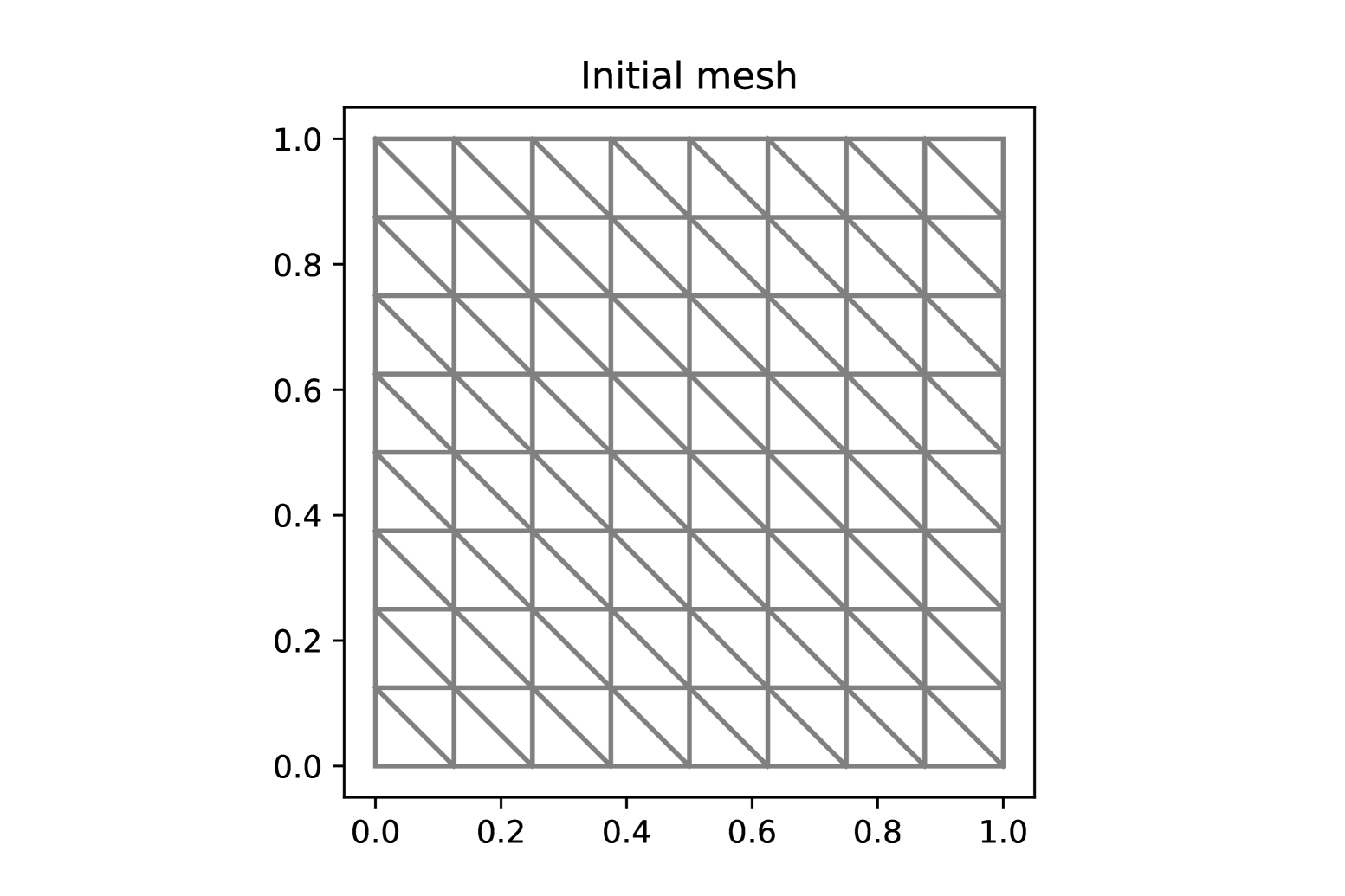
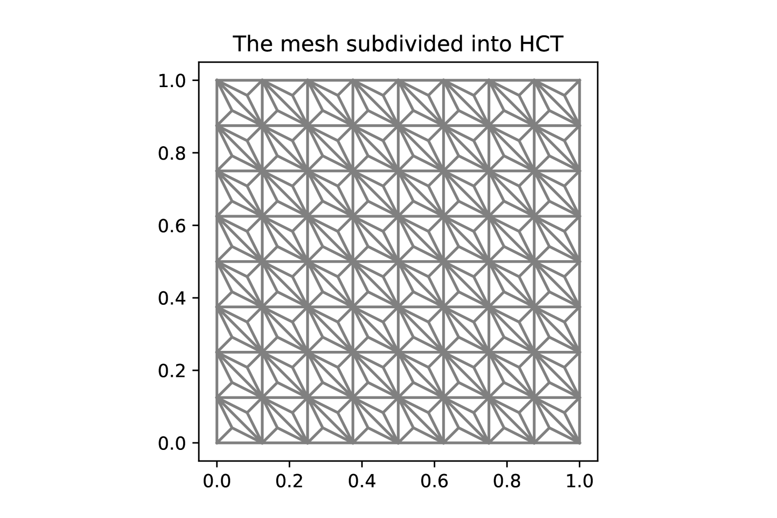
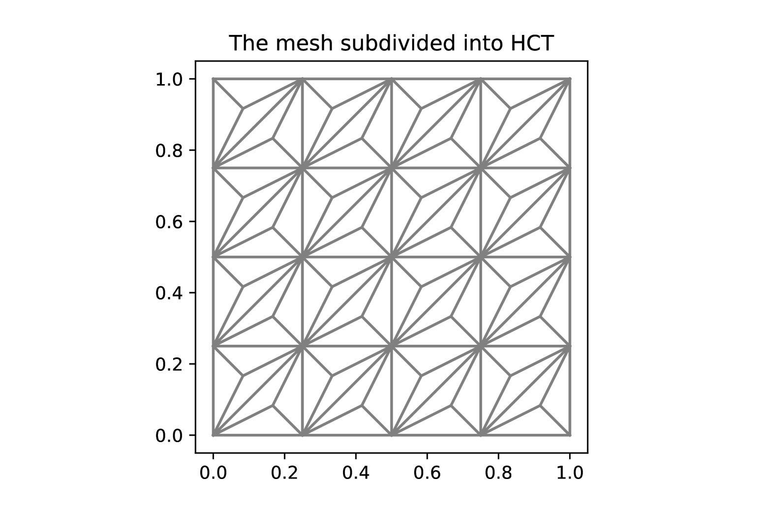
We use the FEniCs software [2], drawing inspiration from the work presented in the report [36]. For the unit square domain $\Omega=]0,1[^{2}$, we generate an initial triangulation (see Figure 6) and subsequently a Hsieh-Clough-Tocher mesh (see Figure 6). Considering a synthetic solution $u_{e}(x,y)=x^{2}(1-x)^{2}y^{2}(1-y)^{2}$ that satisfies the boundary conditions, we implement the following iterative fixed-point scheme with an initial solution $u^{0}_{h}=0.0069$:

(5.1) $$\begin{cases}\text{ Find }u^{n+1}_{h}\in V_{h}\text{ such that},\\ \int_{\Omega}\Delta u^{n+1}_{h}\Delta v_{h}dx+\lambda\int_{\Omega}|u^{n}_{h}|^{2p}u^{n+1}_{h}v_{h}dx=\langle f,v_{h}\rangle\ \forall v_{h}\in V_{h}\end{cases}.$$

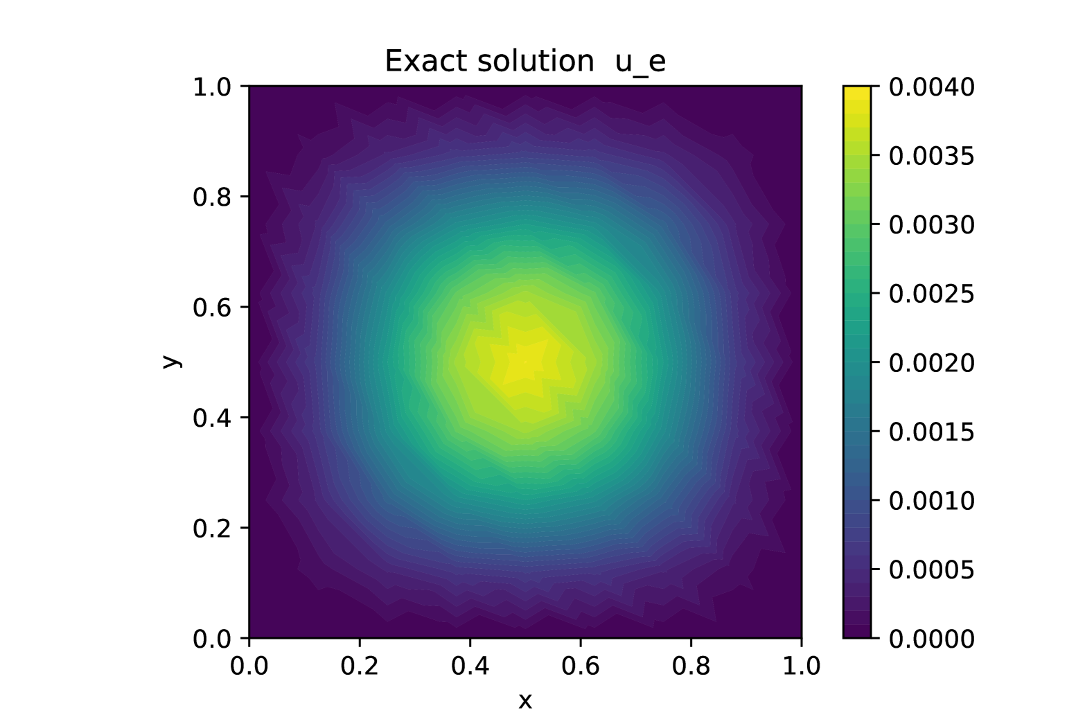
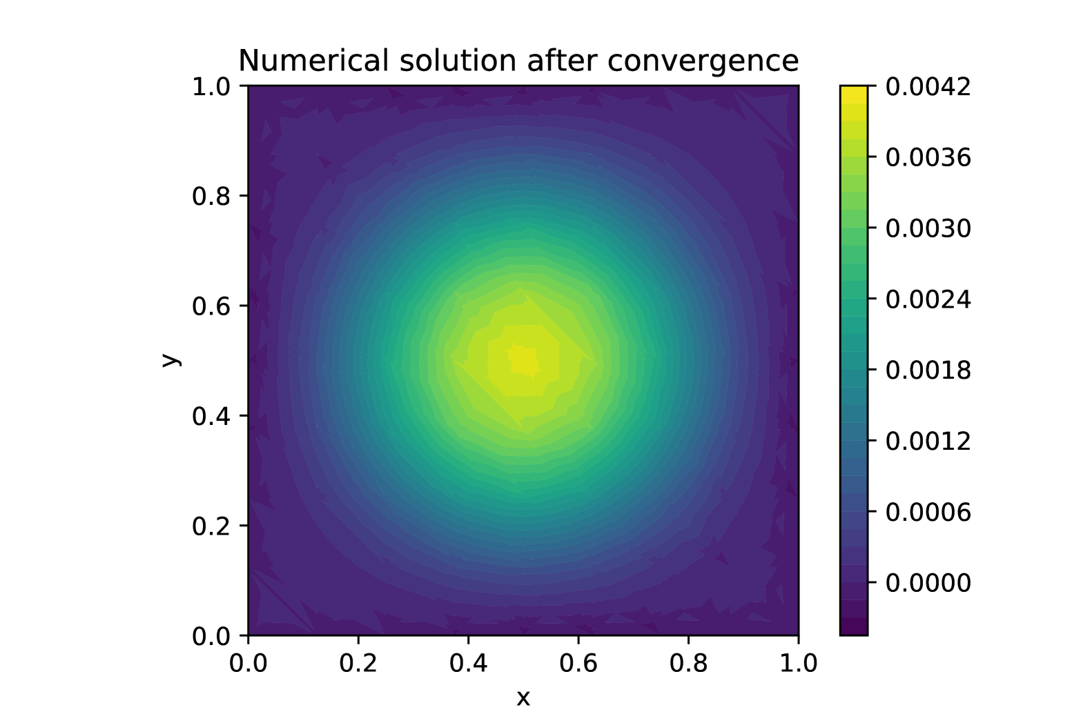
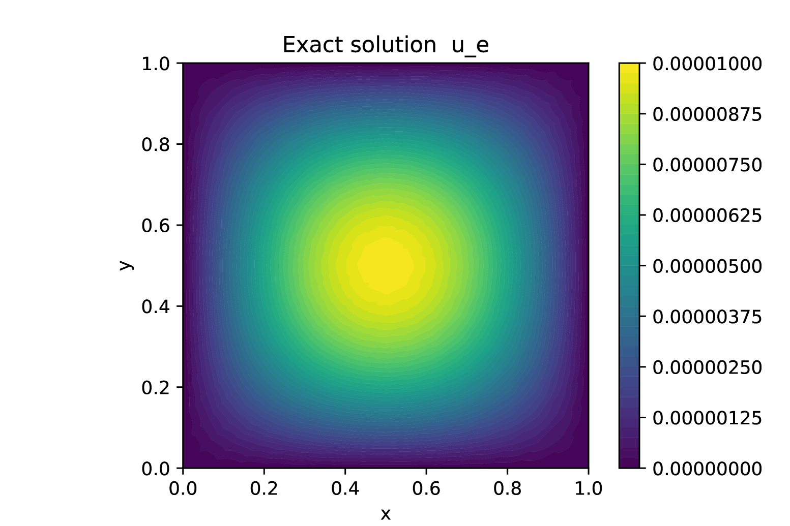
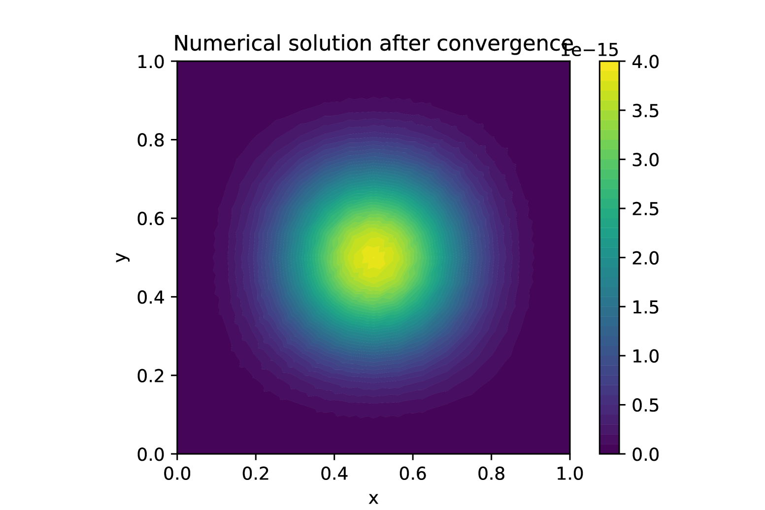
with the classical stopping criterion defined by $err_{L}=|u^{n+1}_{h}-u^{n}_{h}|_{2,\Omega}\leqslant 10^{-7}$. Figure 8 presents the synthetic solution and figure 8 presents the numerical solution after convergence, obtained after a few iterations in a mesh of $384$ cells and $3840$ degrees of freedom with an error in norm $L^{2}(\Omega)$ equal to $0.00010911603387915538$ and in norm $H^{2}_{0}(\Omega)$ equal to $0.005791626721615341$. This result is obtained for $p=1$ and $\lambda=10^{4}$.

Refer to caption
Figure 5. Initial mesh
Refer to caption
Figure 6. The mesh subdivided into HCT
Refer to caption
Figure 7. Exact solution
Refer to caption
Figure 8. Numerical solution

5.2. Test for a priori estimation

For error estimation, the errors are defined as:
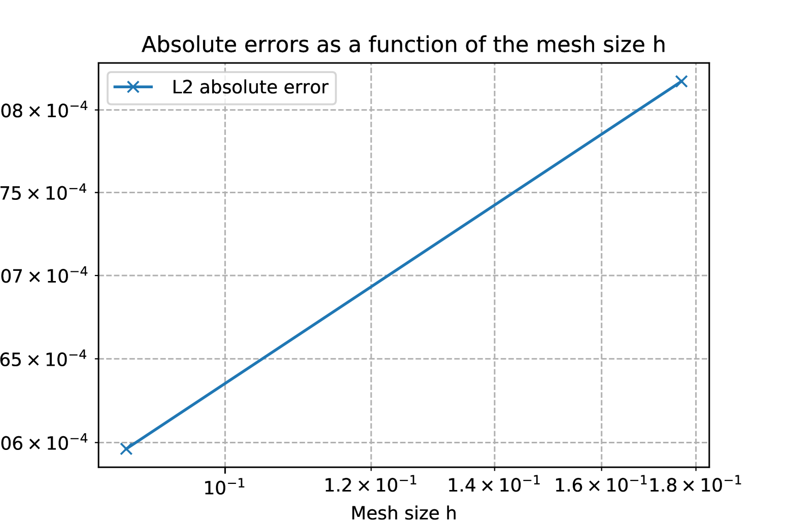
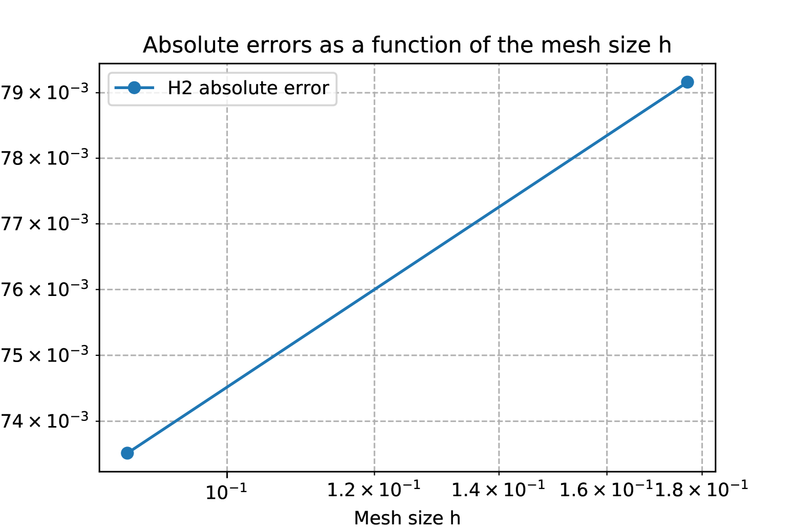
$\displaystyle err_{L2}=\|u-u^{n+1}_{h}\|_{L^{2}(\Omega)},$
$\displaystyle err_{H2}=|u-u^{n+1}_{h}|_{2,\Omega},\text{ where }$
$\displaystyle\|u\|_{L^{2}(\Omega)}=\left(\int_{\Omega}|u|^{2}dx\right)^{1/2}\text{ and }$
$\displaystyle|u|_{2,\Omega}=\left(\sum_{i,j=1}^{n}\left\|\dfrac{\partial^{2}u}{\partial x_{i}\partial x_{j}}\right\|^{2}_{L^{2}(\Omega)}\right)^{1/2}.$

The mapping $u\mapsto\|\Delta u\|_{L^{2}(\Omega)}$ is a norm equivalent to $|\cdot|_{2,\Omega}$ on $H^{2}_{0}(\Omega)$, and the latter is the one used for the computations. The curve in Figure 10 represents the absolute error in the $L^{2}(\Omega)$ norm, while the curve in Figure 10 represents the absolute error in the $H^{2}_{0}(\Omega)$ norm as a function of the mesh size $h$. We tested the algorithm on meshes with $384$ cells and $3840$ degrees of freedom, up to meshes with $1536$ cells and $15360$ degrees of freedom, for $\lambda=10^{4}$ and $p=1$.

Refer to caption
Figure 9. L2 absolute error curve $err_{L2}$.
Refer to caption
Figure 10. H2 absolute error curve $err_{H2}.$
Remark 5.1.

We observe that the error decreases as the discretization step tends to zero, with a slope of order $2.05$. This confirms the theoretical results and the second-order convergence established theoretically in the case of HCT meshes.

$p=1$ $p=2$ $p=3$ $p=10$
$\lambda=10^{-1}$ $0.05791626760487744$ $0.05791626760385732$ $0.05791626760385092$ $0.0579162676038548$
$\lambda=10^{2}$ $0.057916267600419936$ $0.057916267603858866$ $0.05791626760385854$ $0.0579162676038548$
$\lambda=10^{3}$ $0.057916267565529256$ $0.057916267603424186$ $0.05791626760385557$ $0.0579162676038548$
$\lambda=10^{4}$ $0.05791626721615341$ $0.057916267604456347$ $0.05791626760386138$ $0.0579162676038548$
$\lambda=10^{5}$ $0.05791626372236575$ $0.05791626760443946$ $0.057916267603848444$ $0.0579162676038548$
$\lambda=10^{6}$ $0.05791622878463318$ $0.057916267603997006$ $0.057916267603853336$ $0.0579162676038548$
$\lambda=10^{7}$ $0.057915879422095966$ $0.0579162676001085$ $0.05791626760385226$ $0.0579162676038548$
$\lambda=10^{8}$ $0.05790517600316137$ $0.057916267561317444$ $0.05791626760312156$ $0.0579162676038548$
$\lambda=10^{9}$ $div$ $0.05791626717354878$ $0.05791626760378498$ $0.0579162676038548$
$\lambda=10^{10}$ $div$ $0.057916263295906455$ $0.05791626760432593$ $0.0579162676038548$
Table 4. $err_{H2}=|u-u^{n+1}_{h}|_{2,\Omega}$

We denote ’div’ when the scheme does not converge after the maximum number of iterations.
The table 4 shows that the convergence of the iterative scheme indeed depends on the values of $p$ and $\lambda$. This confirms the theoretical result established in Theorem 3.2.

5.3. Test for a posteriori estimation

In this case, we consider the synthetic solution $u(x,y)=\sin(\pi x)\sin(\pi y)$ defined on the domain $\Omega=(0,1)^{2}$, which satisfies the boundary conditions. We implement the iterative fixed-point scheme 5.1. Let $u^{n+1}_{h}$ be the unique solution of 5.1. Then, the a posteriori error indicators are locally defined by:

(5.2) $$\eta^{(D)}_{n}:=\left(\sum_{K\in\mathcal{T}_{h}}[\eta^{(D)}_{K,n}]^{2}\right)^{1/2},$$
(5.3) $$\eta^{(L)}_{n}:=\left(\sum_{K\in\mathcal{T}_{h}}[\eta^{(L)}_{K,n}]^{2}\right)^{1/2},$$

where $\eta^{(D)}_{K,n}=\displaystyle h^{2}_{K}\|f_{h}-\Delta^{2}u^{n+1}_{h}-\lambda|u^{n}_{h}|^{2p}u^{n}_{h}\|_{L^{2}(K)}\\ \\ +\displaystyle\sum_{e\in\varepsilon(K)}\|\Delta u^{n+1}_{h}\|_{L^{2}(e)}+\displaystyle\frac{1}{2}\sum_{e\in\varepsilon(K)}h^{3/2}_{e}\|[\frac{\partial(\Delta u^{n+1}_{h})}{\partial n}]\|_{L^{2}(e)}$, denotes the discretization error indicator, while $\eta^{(L)}_{K,n}=\lambda h^{2}_{K}|u^{n}_{h}-u^{n+1}_{h}|_{2,K}$ represents the linearization error indicator. Let $\gamma$ be a positive parameter. We introduce a new linearization stopping criterion used in [26] as follows:

(5.4) $$\eta^{(L)}_{n}\leqslant\gamma\eta^{(D)}_{n}$$

and the classical stopping criterion

(5.5) $$\eta^{(L)}_{n}\leqslant 10^{-5}.$$

Next, we choose an arbitrary initial approximation $u^{0}_{h}$, and we introduce the following iterative algorithm: For $n\in\mathbb{N}$.

  1. (1)

    Given $u^{n}_{h}$

    1. (a)

      we solve the problem to compute $u^{n+1}_{h}$.

    2. (b)

      we calculate $\eta^{(D)}_{n}$ and $\eta^{(L)}_{n}$.

  2. (2)

    If the linearization error satisfies the stopping criteria 4.20 or 4.21, we terminate the iteration loop and proceed to step $(3)$; otherwise, we repeat step $(1)$.

  3. (3)

    For mesh adaptation:

    1. (a)

      If $\eta^{(D)}_{n}$ is below a specified tolerance $\varepsilon$, we stop the algorithm,

    2. (b)

      otherwise, we perform mesh adaptation, which can be described as follows: Let $\displaystyle\bar{\eta_{n}}^{(D)}=\frac{1}{n_{t}}\sum_{K\in\mathcal{T}_{h}}\eta^{(D)}_{K,n}$ (where $n_{t}$ is the number of triangles in the mesh) on a triangle $K$ of the mesh,

      1. (i)

        if $\eta^{(D)}_{K,n}$ is much smaller than $\bar{\eta_{n}}^{(D)}$, we coarsen the mesh around $K$.

      2. (ii)

        if $\eta^{(D)}_{K,n}$ is much larger than $\bar{\eta_{n}}^{(D)}$, we refine the mesh around $K$.

    3. (c)

      Subsequently, we return to step $(1)$.

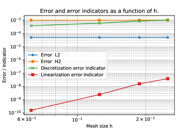
Using the criteria based on the local error indicators 5.4 and 5.5, we achieved convergence, and figure 12 displays the numerical solution after convergence compared to the exact solution presented in figure 12. This result is very satisfactory for $\lambda=10^{6}$ and $p=1$, highlighting once again the effectiveness of local error indicators in the numerical resolution of PDEs. Moreover, figure 13 presents the curve describing the evolution of the two errors and the two error indicators as a function of the discretization step size. Table 5 shows the repartition of $err_{H2}$ and $\eta^{(D)}_{n}$ values as a function of $h$.

Refer to caption
Figure 11. Exact solution
Refer to caption
Figure 12. Numerical solution
Refer to caption
Figure 13. Curve Error/ Indicator
$h$ $err_{H2}=|u-u^{n+1}_{h}|_{2,\Omega}$ $\eta^{(D)}_{n}$ $\eta^{(L)}_{n}$ $\dfrac{\left([\eta^{(D)}_{n}]^{2}+[\eta^{(L)}_{n}]^{2}\right)^{\frac{1}{2}}}{err_{H2}}$
$0.25$ $0.0010227068705228558$ $0.0010359541676476713$ $4.7967065729477115e-08$ $1.0129531722306075$
$0.1875$ $0.0010103485949389303$ $0.0008563221777400873$ $3.145699344479001e-08$ $0.8475512141130194$
$0.125$ $0.000996339947451816$ $0.0005881536238968676$ $1.2210650637519503e-08$ $0.590314205033984$
$0.0625$ $0.0009893373045555425$ $0.00038291768460119846$ $3.159212355349324e-09$ $0.3870446235586514$
Table 5. Repartition of $err_{H2}$ values according $\eta^{(D)}_{n}$ and $\eta^{(L)}_{n}$

Remark 5.2.

We observe that the results obtained in Figure 13 and Table 5 confirm the theoretical results established, demonstrating the reliability and efficiency of the family of local indicators.

5.4. Mesh adaptation

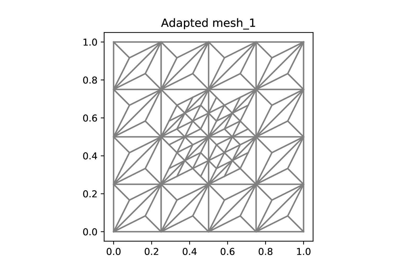
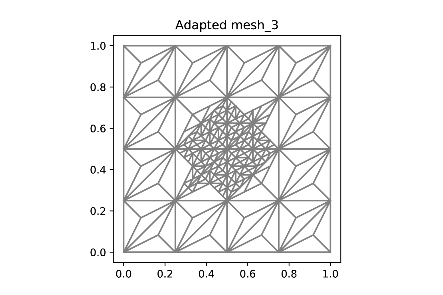
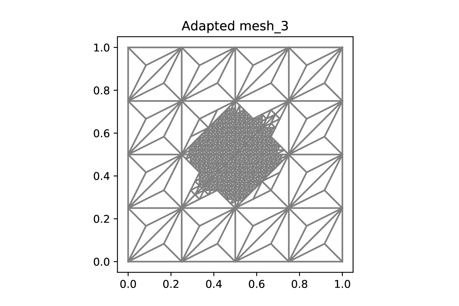
In this subsection, we illustrate the evolution of the mesh adaptation. Starting from an initial HCT mesh (Figure 15), Figures 15, 17, and 17 show the progression of the mesh over the iterations. A significant concentration of mesh adaptation is observed in the region where the solution is non-zero.

Refer to caption
Figure 14. Initial mesh HCT: 96 cells
Refer to caption
Figure 15. First adapted mesh: 144 cells
Refer to caption
Figure 16. Second adapted mesh: 300 cells
Refer to caption
Figure 17. Third adapted mesh: 894 cells

5.5. Discussions

In this subsection, we present the observations from the numerical tests and provide a discussion around them. The initial mesh (Figure 6) is a triangulation of the domain $\Omega=]0;1[^{2}$ and the figure (Figure 6) is the HCT mesh generated from this initial triangulation, while the adapted meshes(Figures 15 to 17) show a strong concentration in the areas where the solution presents significant variations. The obtained numerical solution (Figures 8 and 12) is visually close to the exact solution (Figures 8 and 12), with a rapid convergence after a few iterations. The error curves (Figures 10 and 10) show that the errors decrease monotonically with the mesh step $h$, and that of the figure (Figure13) presents the correlation between the error indicators and the errors. The analysis of the table 4 reveals that the values of the error $|u-u_{h}^{n+1}|_{2,\Omega}$ show a notable dependence on the parameters $p$ and $\lambda$ and that of the table 5 presents the distribution of the error indicators $\eta^{(D)}_{n}$ and of the errors $|u-u^{n+1}_{h}|_{2,\Omega}$ which shows a strong decrease with the mesh refinement.

The numerical results presented in this study highlight several key aspects that demonstrate their importance, both theoretically and practically. We can discuss:

  1. (1)

    Validation of theoretical predictions: The results confirm the theoretical predictions on second-order convergence for HCT meshes. This validation is essential because it ensures that the adopted methodology (HCT elements, error indicators, iterative scheme) is consistent with the established theoretical properties.

  2. (2)

    Effectiveness of a posteriori error estimators: The a posteriori error estimators, $\eta^{(D)}_{n}$ and $\eta^{(L)}_{n}$, were found to be crucial in establishing a stopping criterion based on the balance between discretization and linearization errors that proved robust in handling iterative convergence. They allowed identifying regions requiring mesh refinement. The efficient use of these indicators reduces computational costs while maintaining high accuracy, which is essential for complex nonlinear problems.

  3. (3)

    Impact of mesh adaptation: Mesh adaptation shows a concentration of cells in areas where the solution presents strong variations. This behavior is illustrated by the evolution of the mesh figures. The approach guarantees an optimal allocation of computational resources, making the method competitive even for complex problems.

6. Summary

We analyzed a posteriori residual error estimators of a fixed point iterative algorithm for the plate bending problem perturbed by a nonlinear term. This analysis allowed us to identify two sources of error: the discretization error and the linearization error. The local error indicators obtained are both reliable and efficient. The numerical results obtained fully corroborate the theoretical predictions, thereby validating the coherence and relevance of the proposed model. They demonstrate the efficiency, accuracy, and robustness of the developed method. Moreover, they provide strong experimental validation of the theoretical concepts, positioning this approach as a promising solution for complex nonlinear modeling problems. Many issues remain to be addressed in this area, let us mention other methods, namely, ADINI’s element [39] or nonconforming VIRTUAL element method for plate bending problems recently developed in [31].

7. Acknowledgments

We are thankful to the editor and the anonymous reviewers for many valuable suggestions to improve this paper.

References

  • [1] Adams, R.A. Sobolev spaces, Acadamic Press, INC, Waltham (1978)
  • [2] APA : Logg, A., Mardal, K.-A., Wells, G., and others. (2012). Automated Solution of Differential Equations by the Finite Element Method: The FEniCS Book (Vol. 84). Springer. https://doi.org/10.1007/978-3-642-23099-8
  • [3] S. M. Allen and J. W. Cahn. Ground state structures in ordered binary alloys with second neighbor interactions, Acta Metallurgica, 20(3):423-433, 1972.
  • [4] J. H. Argyris, I. Fried and D. W. Scharpf, The TUBA family of plate elements for the matrix displacement method, Aeronaut, J. Roy. Aeronaut. Soc., 72 (1968), 701-709.
  • [5] J. H. Argyris and D. W. Scharpf, Some general considerations on the natural mode technique, part 1 : Small displacements, Aeronaut, J. Roy. Aeronaut. Soc., 73 (1969), 218-226.
  • [6] K. Bell, A refined triangular plate bending finite element, Internat. J. Numer. Methods Engng., 1 (1969), 101–122.
  • [7] A. Bendali, Méthode des éléments finis , Toulouse, 2013
  • [8] Babuška, I., Rheinboldt, W.C. Error estimates for adaptive finite element computations, SIAM J. Numer. Anal. 4, 736–754 (1978)
  • [9] F. Brezzi and P. A. Raviart, Mixed finite element methods for 4th order elliptic equations, École Polytechnique, Rapport Interne No 9, mai 1976.v
  • [10] Brezzi, F., Rappaz, J., Raviart, P.-A. Finite dimensional approximation of nonlinear problems, part I: Branches of Nonsingular Solutions, Numer. Math. 36, 1–25 (1980).
  • [11] Brezis H.: Analyse Fonctionnelle, Théorie et Applications, Éditions Masson, Paris 1987.
  • [12] Chaillou, A.-L., Suri, M. Computable error estimators for the approximation of nonlinear problems by linearized models, Comput. Methods Appl. Mech. Eng. 196, 210–224 (2006)
  • [13] Chaillou, A.-L., Suri, M. A posteriori estimation of the linearization error for strongly monotone nonlinear operators, Comput. Methods Appl. Mech. Eng. 205, 72–87 (2007)
  • [14] Georges DJOUMNA Méthodes d’interpolation dans la résolution semi-Lagrangienne par éléments finis, des équations de SAINT-VENANT, PhD thesis,Université LAVAL QUÉBEC, 2006.
  • [15] J. W. Cahn and J. E. Hilliard. Free energy of a nonuniform system, I. Interfacial free energy. J. Chem. Phys, 28(2): 258-267, 1958.
  • [16] J.W. Cahn. On spinodal decomposition, Acta Metallurgica, 9(9):795-801, 1961.
  • [17] P. G. Ciarlet, Numerical Analysis of the Finite Element Method, Séminaires de Mathématiques Supérieures, Presses de l’Université de Montréal, 1975.
  • [18] P. G. Ciarlet and R. GLOWINSKI, Dual itérative techniques for solving a finite element approximation of the biharmonic équation, Computer Methods in Applied Mechanics and Engineering, 5,1975, p. 277–295.
  • [19] P. G. Ciarlet, P. A. Raviart, Interpolation theory over curved éléments with applications to finite element methods, Computer Methods in Applied Mechanics and Engineering, 1, 1972, p. 217–249.
  • [20] P. G. Ciarlet, P. A. Raviart, The combined effect of curved boundaries and numerical intégration in isoparametric finite element methods, 409–474, The Mathematical Foundations of the Finite Element Method with Applications to Partial Dijferential Equations, Ey. A- K. Aziz., Acayemic Press, 1972.
  • [21] P. G. Ciarlet, P. A. Raviart, A mixed finite element method for the biharmonic équation, 125–145, Mathematical Aspects of Finite Eléments in Partial Differential Equations, Academie Press, 1974.
  • [22] Philippe G. Ciarlet, Sur l’élément de clough et tocher. ESAIM : Mathematical Modelling and Numerical Analysis -Modélisation Mathématique et Analyse Numérique, 8(R2) :19–27, 1974
  • [23] Philippe G. Ciarlet. Interpolation error estimates for the reduced hsieh-clough-tocher triangle. Mathematics of Computation, 32(142) :335–344, 1978.
  • [24] P h . Clément approimation by finite element function using local regularization , RAIRO (9 e année, août 1975, R-2, p 77–84)
  • [25] Christine Bernardi, L’analyse a posteriori et ses applications, Laboratoire Jacques-Louis Lions, C.N.R.S. et Université Pierre et Marie Curie
  • [26] Christine Bernardi, Jad Dakroub, Gihane Mansour and Tony Sayah A posteriori analysis of iterative algorithms or a nonlinear problem, J.Sci.Comput, DOI 10.1007/s10915-014-9980-4,2015
  • [27] El Alaoui, L., Ern, A., Vohralík, M. Guaranteed and robust a posteriori error estimate and balancing discretization and linearization errore for monotone non linear problems, Comput. Methods Appl. Mech. Eng. 200, 2782–2795 (2011) (1980)
  • [28] Emily C., Christophe D. Cours : Analyse fonctionnelle, Master1-Maths, (2014-2015)
  • [29] S. K Esavan M. Vanninathan Sur une méthode d’éléments finis mixte pour l’équation biharmonique RAIRO. Analyse numérique, tome 11, (1977), p. 255–270.
  • [30] Kavian, O.: Introduction à la théorie des points critiques et applications aux problèmes elliptiques, Springer, Berlin-Heidelberg (1993).
  • [31] Jikun Zhao, Shaochun Chen and Bei Zhang, The nonconforming virtual element method for plate bending problems, Mathematical Models and Methods in Applied Sciences (Word Scientific), doi 10.1142/S02182025165005, 2016.
  • [32] K. W. Houédanou. Analyse d’erreur a posteriori pour quelques méthodes d’éléments finis mixtes pour le problème de transmission Stokes-Darcy: Discrétisations isotrope et anisotrope, PhD thesis, Université d’Abomey-Calavi, 2015.
  • [33] B. Lucquin, Équations aux dérivées partielles et leurs approximations, Collection Mathématiques à l’université, 240 pages, 2004.
  • [34] Marie Martin, Fluids modeling of fusion plasmas : approximation with C1 finite element of Bell. Theses, Université Nice Sophia Antipolis, June 2013
  • [35] Michel Bernadou and Kamal Hassan, Basis Functions for General HSIEH-CLOUGH-TOCHER Triangles, Complete or reduced,Institut National de Recherche en Informatique et en Automatique, Rapport de Recherche numéro 5, Janvier 1980.
  • [36] Michel Bernadou, Jean-Marie Boisserie, and Kamal Hassan, Sur l’implémentation des éléments finis de Hsieh-Clough-Tocher complet et réduit. Research Report RR-0004, INRIA, 1980.
  • [37] R.W. Clough and J.L. Tocher. Finite element stiness matrices for analysis of plates in bending, In Proc. Conf. Matrix Methods in Struct. Mech. , Air Force Inst of Tech., Wright Patterson A.F Base, Ohio, October 1965.
  • [38] Serge Nicaise, Analyse numérique et équations aux dérivées partielles, Cours et problèmes résolus, Édition DUNOD Paris 2000.
  • [39] Shaochun Chen, Yongcheng Zhao and Dongyang Shi, Anisotropic interpolation with application to nonconforming elements, Applied Numerical Mathematics (Elsevier), 49 : 135–152, 2004.
  • [40] Soglo Ambroise, Houédanou Koffi Wilfrid and Adetola Jamal, Mass Transportation approach for parabolic $p$-Biharmonic Equations, Aust. J. Math. Anal. Appl., 1 (21):1–23, 2024.
  • [41] Verfürth, R. A posteriori error estimation techniques for finite element methods, Oxford University Press, Oxford (2013)