When Do Transformers Outperform Feedforward and
Recurrent Networks? A Statistical Perspective

Abstract

Theoretical efforts to prove advantages of Transformers in comparison with classical architectures such as feedforward and recurrent neural networks have mostly focused on representational power. In this work, we take an alternative perspective and prove that even with infinite compute, feedforward and recurrent networks may suffer from larger sample complexity compared to Transformers, as the latter can adapt to a form of dynamic sparsity. Specifically, we consider a sequence-to-sequence data generating model on sequences of length $N$, in which the output at each position depends only on $q$ relevant tokens with $q\ll N$, and the positions of these tokens are described in the input prompt. We prove that a single-layer Transformer can learn this model if and only if its number of attention heads is at least $q$, in which case it achieves a sample complexity almost independent of $N$, while recurrent networks require $N^{\Omega(1)}$ samples on the same problem. If we simplify this model, recurrent networks may achieve a complexity almost independent of $N$, while feedforward networks still require $N$ samples. Consequently, our proposed sparse retrieval model illustrates a natural hierarchy in sample complexity across these architectures.

1 Introduction

Transformers [51], neural network architectures that are composed of attention and feedforward blocks, are now at the backbone of large models in machine learning across many different tasks [43, 17, 13]. The theoretical efforts surrounding the success of Transformers have so far demonstrated various capabilities like in-context learning [3, 49, 9, 59, 27, and others] and chain of thought along with its benefits [22, 37, 32, 28, and others] in various settings. There are fewer works that provide specific benefits of Transformers in comparison with feedforward and recurrent architectures. On the approximation side, there are tasks that Transformers can solve with size logarithmic in the input, while other architectures such as recurrent and feedforward networks require polynomial size [44, 45]. Based on these results, [55] showed a separation between Transformers and feedforward networks by providing further optimization guarantees for gradient-based training of Transformers on a sparse token selection task.

While most prior works focused on the approximation separation between Transformers and feedforward networks, in this work we focus on a purely statistical separation, and ask:

What function class can Transformers learn with fewer samples compared to
feedforward and recurrent networks, even with infinite compute?

[21] approached the above problem with random features, where the query-key matrix for the attention and the first layer weights for the two-layer feedforward network were fixed at random initialization. However, this only presents a partial picture, as neural networks can learn a significantly larger class of functions once “feature learning” is allowed, i.e., parameters are trained to adapt to the structure of the underlying task [6, 10, 19, 8, 18, 1, 35].

We evaluate the statistical efficiency of transformers and alternative architectures by characterizing how the sample complexity depends on the input sequence length. A benign sequence length dependence (e.g., sublinear) signifies the ability to achieve low test error in longer sequences, which is intuitively connected to the length generalization capability [4]. While Transformers have demonstrated this ability in certain structured logical tasks, they fail in other simple settings [58, 29]. Our generalization bounds for bounded-norm Transformers — along with our contrasts to RNNs and feedforward neural networks — provide theoretical insights into the statistical advantages of Transformers and lay the foundation for future rigorous investigations of length generalization.

Statistical Model	Feedforward	RNN	Transformer
Simple-$q\mathrm{STR}$	✗  (Theorem 6)	✓  (Theorem 7)	✓  (Theorem 4)
$q\mathrm{STR}$	✗  (Theorem 6)	✗  (Theorem 9)	✓  (Theorem 4)

Table 1: Summary of main contributions (see Theorem 1). ✓ indicates a sample complexity upper bound that is almost sequence length-free (up to polylogarithmic factors). ✗ indicates a lower bound of order $N^{\Omega(1)}$.

1.1 Our Contributions

We study the $q$-Sparse Token Regression ($q\mathrm{STR}$) data generating model, a sequence-to-sequence model where the output at every position depends on a sparse subset of the input tokens. Importantly, this dependence is dynamic, i.e., changes from prompt to prompt, and is described in the input itself. We prove that by employing the attention layer to retrieve relevant tokens at each position, single-layer Transformers can adapt to this dynamic sparsity, and learn $q\mathrm{STR}$ with a sample complexity almost independent of the length of the input sequence $N$, as long as the number of attention heads is at least $q$. On the other hand, we develop a new metric-entropy-based argument to derive norm and parameter-count lower bounds for RNNs approximating the $q\mathrm{STR}$ model. Thanks to lower bounds on weight norm, we also obtain a sample complexity lower bound of order $N^{\Omega(1)}$ for RNNs. Further, we show that RNNs can learn a subset of $q\mathrm{STR}$ models where the output is a constant sequence, which we call simple-$q\mathrm{STR}$, with a sample complexity polylogarithmic in $N$. Finally, we develop a novel lower bound technique for feedforward networks (FFNs) that takes advantage of the fully connected projection of the first layer to obtain a sample complexity lower bound linear in $N$, even when learning simple-$q\mathrm{STR}$ models. The following theorem and Table 1 summarize our main contributions.

Theorem 1 (Informal).

We have the following hierarchy of statistical efficiency for learning $q\mathrm{STR}$.

• A single-layer Transformer with $H\geq q$ heads can learn $q\mathrm{STR}$ with sample complexity almost independent of $N$, and cannot learn $q\mathrm{STR}$ when $H<q$ even with infinitely many samples.

• RNNs can learn simple-$q\mathrm{STR}$ models with sample complexity almost independent of $N$, but require at least $\Omega(N^{c})$ samples for some absolute constant $c>0$ to learn a generic $q\mathrm{STR}$ model, regardless of their size.

• Feedforward neural networks, regardless of their size, require $\Omega(Nd)$ samples to learn even simple-$q\mathrm{STR}$ models, where $d$ is input token dimension.

We experimentally validate the intuitions from Theorem 1 in Figure 1, where we observe that on a $1\mathrm{STR}$ task, both FFNs and RNNs suffer from a large sample complexity for larger $N$. However, for a simple-$1\mathrm{STR}$ model RNNs perform closer to Transformers with a much milder dependence on $N$ compared to FFNs.

1.2 Related Work

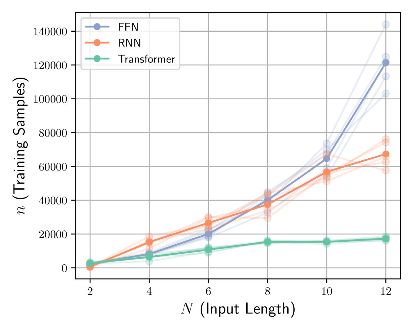
(a) Sample complexity (1STR)

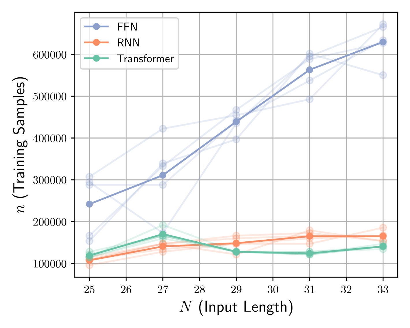
(b) Sample complexity (Simple-1STR)

Figure 1: Number of samples required to reach a certain test MSE loss threshold while training with online AdamW. We consider (1(a)) the $1\mathrm{STR}$ model with loss threshold $0.7$ and (1(b)) the simple-$1\mathrm{STR}$ model with loss threshold $0.02$, averaged over 5 experiments. We use a linear link function, standard Gaussian input, $d=10$ and $d_{e}=\lfloor 5\log(N)\rfloor$. Positional encodings are sampled uniformly from the unit hypercube. This observation is consistent with Theorem 1.

While generalization is a fundamental area of study in machine learning theory, theoretical work on the generalization capabilities of Transformers remains relatively sparse. Some works analyze the inductive biases of self-attention through connections to max-margin SVM classifiers [48]. Others quantify complexity in terms of the simplest programs in a formal language (such as the RASP model of [57]) that solve the task and relate that to Transformer generalization [58, 16]. The most relevant works to our own are [20, 47, 46], which employ covering numbers to bound the sample complexity of deep Transformers with bounded weights. They demonstrate a logarithmic scaling in the sequence length, depth, and width and apply their bounds to the learnability of sparse Boolean functions. We refine these covering number bounds to better characterize generalization in sequence-to-sequence learning with dynamic sparsity [44]. Our problems formalize long-context reasoning tasks, extending beyond simple retrieval to include challenges like multi-round coreference resolution [50].

Expressivity of Transformers.

The expressive power of Transformers has been extensively studied in prior works. Universality results establish that Transformers can approximate the output of any continuous function or Turing machine [56, 52], but complexity limitations remain for bounded-size models. Transformers with fixed model sizes are unable to solve even regular languages, such as Dyck and Parity [7, 23]. Further work [e.g. 36] relates Transformers to boolean circuits to establish the hardness of solving tasks like graph connectivity with even polynomial-width Transformers. Additionally, work on self-attention complexity explores how the embedding dimension and number of heads affects the ability of attention layers to approximate sparse matrices [30], recover nearest-neighbor associations [5], and compute sparse averages [44]. The final task closely resembles our $q$STR model and has been applied to relate the capabilities of deep Transformers to parallel algorithms [45]. Several works [e.g. 25, 12, 53] introduce sequential tasks where Transformers outperform RNNs or other state space models in parameter-efficient expressivity. We establish similar architectural separations with an added focus on differentiating the generalization capabilities of Transformers, RNNs, and FFNs.

Statistical Separation.

Our work is conceptually related to studies on feature learning and adaptivity in feedforward networks, particularly in learning models with sparsity and low-dimensional structures. Prior work has analyzed how neural networks and gradient-based optimization introduce inductive biases that facilitates the learning of low-rank and low-dimensional functions [33, 54, 14, 34, 39]. These studies often demonstrate favorable generalization properties based on certain structures of the solution such as large margin or low norm [11, 38, 40, 54]. Our goal is to extend efficient learning of low-dimensional concepts to sequential architectures, ensuring sample complexity remains efficient in both input dimension $d$ and context length $N$. Our approach, motivated by [44, 55], suggests that $q$STR is a sequential model whose sparsity serves as a low-dimensional structure, making it the primary determinant of generalization complexity for Transformers.

Notation.

For a natural number $n$, define $[n]\coloneqq\{1,\ldots,n\}$. We use $\mathopen{}\mathclose{{\left\|{\cdot}}}\right\|_{p}$ to denote the $\ell_{p}$ norm of vectors. For a matrix $\boldsymbol{A}\in\mathbb{R}^{m\times n}$, $\mathopen{}\mathclose{{\left\|{\boldsymbol{A}}}}\right\|_{p,q}\coloneqq\big{\|}\big{(}\mathopen{}\mathclose{{\left\|{\boldsymbol{A}_{:,1}}}}\right\|_{p},\ldots,\mathopen{}\mathclose{{\left\|{\boldsymbol{A}_{:,n}}}}\right\|_{p}\big{)}\big{\|}_{q}$, and $\mathopen{}\mathclose{{\left\|{\boldsymbol{A}}}}\right\|_{\mathrm{op}}$ denotes the operator norm of $\boldsymbol{A}$. We use $a\lesssim b$ and $a\leq\mathcal{O}(b)$ interchangeably, which means $a\leq Cb$ for some absolute constant $C$. We similarly define $\gtrsim$ and $\Omega$. $\tilde{\mathcal{O}}$ and $\tilde{\Omega}$ hide multiplicative constants that depend polylogarithmically on problem parameters. $\sigma$ denotes the ReLU activation.

2 Problem Setup

Statistical Model.

In this paper, we will focus on the ability of different architectures for learning the following data generating model.

Definition 2 ($q$-Sparse Token Regression).

Suppose $\boldsymbol{p},\boldsymbol{y}\sim\mathcal{P}$ where

$$\boldsymbol{p}=\mathopen{}\mathclose{{\left(\begin{pmatrix}\boldsymbol{x}_{1}\\ \boldsymbol{t}_{1}\end{pmatrix},\ldots,\begin{pmatrix}\boldsymbol{x}_{N}\\ \boldsymbol{t}_{N}\end{pmatrix}}}\right),$$

$\boldsymbol{t}_{i}\in[N]^{q}$ and $\boldsymbol{x}_{i}\in\mathbb{R}^{d}$ for $i\in[N]$. In the $q$-sparse token regression ($q$STR) data generating model, the output is given by $\boldsymbol{y}=(y_{1},\ldots,y_{N})^{\top}\in\mathbb{R}^{N}$, where

$$y_{i}=g(\boldsymbol{x}_{t_{i1}},\ldots,\boldsymbol{x}_{t_{iq}}),$$

for some $g:\mathbb{R}^{qd}\to\mathbb{R}$. We call this model simple-$q\mathrm{STR}$ if the data distribution is such that $\boldsymbol{t}_{i}=\boldsymbol{t}$ for all $i\in[N]$ and some $\boldsymbol{t}$ drawn from $[N]^{q}$.

The above defines a class of sequence-to-sequence functions, where the label at position $i$ in the output sequence depends only on a subsequence of size $q$ of the input data, determined by the set of indices $\boldsymbol{t}_{i}$. $\boldsymbol{p}$ in the above definition denotes the prompt or context. Given the large context length of modern architectures, we are interested in a setting where $q\ll N$. In this setting, the answer at each position only depends on a few tokens, however the tokens it depends on change based on the context. Therefore, we seek architectures that are adaptive to this form of dynamic sparsity in the true data generating process, with computational and sample complexity independent of $N$. As a special case, choosing the link function $g$ above as the tokens’ mean recovers the sparse averaging model proposed in [44], where the authors demonstrated a separation in terms of approximation power between Transformers and other architectures.

To obtain statistical guarantees, we will impose mild moment assumptions on the data, amounting to subGaussian inputs and link functions growing at most polynomially.

Assumption 1.

Suppose $\operatorname{\mathbb{E}}\mathopen{}\mathclose{{\left[{\mathopen{}\mathclose{{\left\|{\boldsymbol{x}_{i}}}}\right\|^{r}}}}\right]^{1/r}\leq\sqrt{C_{x}dr}$ and $\operatorname{\mathbb{E}}\mathopen{}\mathclose{{\left[{\mathopen{}\mathclose{{\left|y_{i}}}\right|^{r}}}}\right]^{1/r}\leq\sqrt{C_{y}r^{s}}$ for all $r\geq 1$, $i\in[N]$, and some absolute constants $s\geq 1$ and $C_{x},C_{y}>0$.

Learning the $q\mathrm{STR}$ model requires two steps: 1. extracting the relevant tokens at each position and 2. learning the link function $g$. We are interested in settings where the difficulty of learning is dominated by the first step, therefore we assume $g$ is well-approximated by a two-layer feedforward network.

Assumption 2.

There exist $m_{g}\in\mathbb{N}$, $\boldsymbol{a}_{g},\boldsymbol{b}_{g}\in\mathbb{R}^{m_{g}}$ and $\boldsymbol{W}_{g}\in\mathbb{R}^{m_{g}\times qd}$, such that $\mathopen{}\mathclose{{\left\|{\boldsymbol{a}_{g}}}}\right\|_{2}\leq r_{a}/\sqrt{m_{g}}$, and $\|(\boldsymbol{W}_{g},\boldsymbol{b}_{g})\|_{\mathrm{F}}\leq\sqrt{m_{g}}r_{w}$ for some constants $r_{a},r_{w}>0$, and

$$\sup_{\big{\{}\mathopen{}\mathclose{{\left\|{\boldsymbol{x}_{i}}}}\right\|_{2}\leq\sqrt{Cd\log(nN)},\,\forall i\in[q]\big{\}}}\mathopen{}\mathclose{{\left|g(\boldsymbol{x}_{1},\ldots,\boldsymbol{x}_{q})-\boldsymbol{a}_{g}^{\top}\sigma(\boldsymbol{W}_{g}(\boldsymbol{x}_{1}^{\top},\ldots,\boldsymbol{x}_{q}^{\top})^{\top}+\boldsymbol{b}_{g})}}\right|^{2}\leq\varepsilon_{{\texttt{2NN}}},$$

where $C=3C_{x}e$ and $\varepsilon_{{\texttt{2NN}}}$ is some absolute constant.

Ideally, $\varepsilon_{\texttt{2NN}}$ above is a small constant denoting the approximation error. This assumption can be verified using various universal approximation results for ReLU networks. For example, when $g$ is an additive model of $P$ Lipschitz functions, where each function depends only on a $k$-dimensional projection of the input, the above holds for every $\varepsilon_{\texttt{2NN}}>0$ and $m_{g}=\tilde{\mathcal{O}}\big{(}(P/\sqrt{\varepsilon_{\texttt{2NN}}})^{k}\big{)}$, $r_{a}=\tilde{\mathcal{O}}\big{(}(P/\sqrt{\varepsilon_{\texttt{2NN}}})^{(k+1)/2}\big{)}$, and $r_{w}=1$ (we can always have $r_{w}=1$ by homogeneity) [6].

Empirical Risk Minimization.

While Empirical Risk Minimization (ERM) is a standard abstract learning algorithm to use for generalization analysis, its standard formalizations use risk functions for scalar-valued predictions. Before introducing the notions of ERM that we employ, we first state several sequential risk formulations to evaluate a predictor $\hat{\boldsymbol{y}}_{{\texttt{arc}}}(\cdot;\boldsymbol{\Theta})\in\mathcal{F}_{\texttt{arc}}$ on i.i.d. training samples $\{\boldsymbol{p}^{(i)},{\boldsymbol{y}}^{(i)}\}_{i=1}^{n}$, where arc denotes a general architecture. We define the population risk, averaged empirical risk, and point-wise empirical risk respectively as

$$R^{{\texttt{arc}}}(\boldsymbol{\Theta}) \coloneqq\frac{1}{N}\operatorname{\mathbb{E}}\mathopen{}\mathclose{{\left[{\sum_{j=1}^{N}(\hat{y}_{{\texttt{arc}}}(\boldsymbol{p}^{(i)};\boldsymbol{\Theta})_{j}-y^{(i)}_{j})^{2}}}}\right]=\frac{1}{N}\operatorname{\mathbb{E}}\mathopen{}\mathclose{{\left[{\mathopen{}\mathclose{{\left\|{\hat{\boldsymbol{y}}_{{\texttt{arc}}}(\boldsymbol{p}^{(i)};\boldsymbol{\Theta})-\boldsymbol{y}^{(i)}}}}\right\|_{2}^{2}}}}\right],$$ (2.1)

$$\hat{R}^{{\texttt{arc}}}_{n,N}(\boldsymbol{\Theta}) \coloneqq\frac{1}{nN}\sum_{i=1}^{n}\sum_{j=1}^{N}\big{(}\hat{y}_{{\texttt{arc}}}(\boldsymbol{p}^{(i)};\boldsymbol{\Theta})_{j}-y^{(i)}_{j}\big{)}^{2},$$ (2.2)

$$\hat{R}^{{\texttt{arc}}}_{n}(\boldsymbol{\Theta}) \coloneqq\frac{1}{n}\sum_{i=1}^{n}\big{(}\hat{y}_{{\texttt{arc}}}(\boldsymbol{p}^{(i)};\boldsymbol{\Theta})_{j^{(i)}}-y^{(i)}_{j^{(i)}}\big{)}^{2},$$ (2.3)

where $\{j^{(i)}\}_{i=1}^{n}$ are i.i.d. position indices drawn from $\mathrm{Unif}([N])$.The goal is to minimize the population risk $R^{{\texttt{arc}}}(\boldsymbol{\Theta})$ by minimizing some empirical risk, potentially with weight regularization. We use three formalizations of learning algorithms to prove our results.

1. Constrained ERM minimizes an empirical risk $\hat{R}^{\texttt{arc}}$ subject to the model parameters belonging on some (e.g., norm-constrained) set $\varTheta$. Concretely, let

   $$\hat{\boldsymbol{\Theta}}\in\operatorname*{arg\,min}_{\boldsymbol{\Theta}\in\varTheta}\hat{R}^{{\texttt{arc}}}(\boldsymbol{\Theta}).$$

   Theorem 4 considers constrained ERM algorithms for bounded-weight transformers with point-wise risk $\hat{R}^{{\texttt{TR}}}_{n}(\boldsymbol{\Theta})$, and Theorem 7 uses $\hat{R}^{{\texttt{RNN}}}_{n}(\boldsymbol{\Theta})$ for RNNs. Note that the upper bounds proved for training with point-wise empirical risk $\hat{R}^{\texttt{arc}}_{n}$ readily transfer to training with averaged empirical risk $\hat{R}^{\texttt{arc}}_{n,N}$.

2. Min-norm $\varepsilon$-ERM minimizes the norm of the parameters, subject to sufficiently small loss:

   $$\hat{\boldsymbol{\Theta}}_{\varepsilon}\in\operatorname*{arg\,min}_{\{\boldsymbol{\Theta}:\hat{R}^{{\texttt{arc}}}(\boldsymbol{\Theta})-\min\hat{R}^{{\texttt{arc}}}\leq\varepsilon\}}\mathopen{}\mathclose{{\left\|{\operatorname{vec}(\boldsymbol{\Theta})}}}\right\|_{2}.$$ (2.4)

   Theorem 9 uses min-norm $\varepsilon$-ERM to place a lower bound on the sample complexity of RNNs with $\hat{R}^{{\texttt{RNN}}}_{n}(\boldsymbol{\Theta})$. The two formulations can be related by letting $\varepsilon_{\varTheta}$ denote the risk penalty for restricting parameters to $\varTheta$.

3. Beyond ERM, Theorem 6 also considers stationary points of the averaged or point-wise loss, with $\ell_{2}$ regularization. This learning algorithm is presented in greater detail in Definition 5.

3 Transformers

A single-layer Transformer is composed of an attention layer and a fully connected feedforward network that is applied in parallel to the outputs of attention. In the following, we describe our assumptions on the different components of the Transformer architecture.

Positional encoding.

To break the permutation equivaraince of Transformers, we append positional information to the input tokens. Given a prompt $\boldsymbol{p}$, we consider an encoding given by

$$\boldsymbol{Z}(\boldsymbol{p})=\begin{pmatrix}\boldsymbol{x}_{1}&\ldots&\boldsymbol{x}_{N}\\ \operatorname{enc}(1,\boldsymbol{t}_{1})&\ldots&\operatorname{enc}(N,\boldsymbol{t}_{N})\end{pmatrix}\in\mathbb{R}^{D_{e}\times N},$$

where $\operatorname{enc}:[N]\times[N]^{q}\to\mathbb{R}^{d_{\operatorname{enc}}}$ provides the encoding of the position and of $\boldsymbol{t}_{i}$, and $D_{e}\coloneqq d+d_{\operatorname{enc}}$. We use $\boldsymbol{z}_{i}$ to refer to the $i$th column above. We remark that allowing $\operatorname{enc}$ to take $\boldsymbol{t}_{i}$ as input allows specific encodings of the indices $\boldsymbol{t}_{i}$ that take advantage of the $q\mathrm{STR}$ structure; examples of this have been considered in prior works [55]. In practice, we expect such useful encodings to be learned automatically by previous layers in the Transformer. We remark that for a fair comparison, in our lower bounds for other architectures we allow arbitrary processing of $\boldsymbol{t}_{i}$ in their encoding procedure. To specify $\operatorname{enc}$, we use a set of vectors $\{\boldsymbol{\omega}_{i}\}_{i=1}^{N}$ in $\mathbb{R}^{d_{e}}$ that satisfy the following property.

Assumption 3.

We have $\mathopen{}\mathclose{{\left|\mathopen{}\mathclose{{\left\langle{\boldsymbol{\omega}_{i}},{\boldsymbol{\omega}_{j}}}}\right\rangle}}\right|\leq\frac{1}{2}$ for all $i\neq j$, and $\mathopen{}\mathclose{{\left\|{\boldsymbol{\omega}_{i}}}}\right\|^{2}=1$ for all $i$.

Such a set of vectors can be obtained e.g., by sampling random Rademacher vectors from the unit cube $\{\pm 1/\sqrt{d_{e}}\}^{d_{e}}$, with $d_{e}=\Theta(\log N)$, which is the scaling we assume throughout the paper. We can now define

$$\operatorname{enc}(i,\boldsymbol{t}_{i})=\sqrt{d/q}(\boldsymbol{\omega}_{i},\boldsymbol{\omega}_{t_{i1}},\ldots,\boldsymbol{\omega}_{t_{iq}})^{\top}\in\mathbb{R}^{(q+1)d_{e}},$$

hence $d_{\operatorname{enc}}=(q+1)d_{e}$ and $D_{e}=d+(q+1)d_{e}$. The $\sqrt{d/q}$ prefactor ensures that $\boldsymbol{x}_{i}$ and $\operatorname{enc}(i,\boldsymbol{t}_{i})$ will roughly have the same $\ell_{2}$ norm, resulting in a balanced input to the attention layer.

Multi-head attention.

Given a sequence $\{\boldsymbol{z}_{i}\}_{i=1}^{N}$ where $\boldsymbol{z}_{i}\in\mathbb{R}^{D_{e}}$ with $D_{e}$ as the embedding dimension, a single head of attention outputs another sequence of length $N$ in $\mathbb{R}^{D_{e}}$, given by

$$f_{{\texttt{Attn}}}(\boldsymbol{p};\boldsymbol{W}_{Q},\boldsymbol{W}_{K},\boldsymbol{W}_{V})=\mathopen{}\mathclose{{\left[\sum_{j=1}^{N}\boldsymbol{W}_{V}\boldsymbol{z}_{j}\frac{e^{\mathopen{}\mathclose{{\left\langle{\boldsymbol{W}_{Q}\boldsymbol{z}_{i}},{\boldsymbol{W}_{K}\boldsymbol{z}_{j}}}}\right\rangle}}{\sum_{l=1}^{N}e^{\mathopen{}\mathclose{{\left\langle{\boldsymbol{W}_{Q}\boldsymbol{z}_{i}},{\boldsymbol{W}_{K}\boldsymbol{z}_{l}}}}\right\rangle}}}}\right]_{i\in[N]}.$$

Where $\boldsymbol{W}_{K},\boldsymbol{W}_{Q},\boldsymbol{W}_{V}$ are the key, query, and value projection matrices respectively. We can simplify the presentation by replacing $\boldsymbol{W}_{Q}^{\top}\boldsymbol{W}_{K}$ with a single parameterizing matrix for query-key projections denoted by $\boldsymbol{W}_{\mathrm{QK}}\in\mathbb{R}^{D_{e}\times D_{e}}$, and absorbing $\boldsymbol{W}_{V}$ into the weights of the feedforward layer. This provides us with a simplified parameterization of attention, which we denote by $f_{\texttt{Attn}}(\boldsymbol{p};\boldsymbol{W}_{\mathrm{QK}})$. This simplification is standard in theoretical works (see e.g. [31, 2, 59, 55]). Our main separation results still apply when maintaining separate trainable projections; the above only simplifies the exposition.

We can concatenate the output of $H$ attention heads with separate key-query projection matrices to obtain a multi-head attention layer with $H$ heads. We denote the output of head $h\in[H]$ with $f_{{\texttt{Attn}}}(\boldsymbol{p};\boldsymbol{W}_{\mathrm{QK}}^{(h)})$. The output of the multi-head attention at position $i$ is then given by

$$f_{{\texttt{Attn}}}^{(H)}(\boldsymbol{p};\boldsymbol{W}^{(1)}_{\mathrm{QK}},\ldots,\boldsymbol{W}^{(H)}_{\mathrm{QK}})_{i}=(f_{\texttt{Attn}}(\boldsymbol{p};\boldsymbol{W}^{(1)}_{\mathrm{QK}})_{i},\ldots,f_{\texttt{Attn}}(\boldsymbol{p};\boldsymbol{W}^{(H)}_{\mathrm{QK}})_{i})^{\top}\in\mathbb{R}^{HD_{e}}.$$

We will denote by $\boldsymbol{\Theta}_{\mathrm{QK}}=(\boldsymbol{W}^{(1)}_{\mathrm{QK}},\ldots,\boldsymbol{W}^{(H)}_{\mathrm{QK}})$ the parameters of the multi-head attention.

Finally, a two-layer neural network acts on the output of the attention to generate labels. Given input $\boldsymbol{h}\in\mathbb{R}^{HD_{e}}$, the output of the network is given by

$$f_{{\texttt{2NN}}}(\boldsymbol{h};\boldsymbol{a}_{\texttt{2NN}},\boldsymbol{W}_{\texttt{2NN}},\boldsymbol{b}_{\texttt{2NN}})=\boldsymbol{a}_{\texttt{2NN}}^{\top}\sigma(\boldsymbol{W}_{\texttt{2NN}}\boldsymbol{h}+\boldsymbol{b}_{\texttt{2NN}}),$$

where $\boldsymbol{W}_{\texttt{2NN}}\in\mathbb{R}^{m\times HD_{e}}$ are the first layer weights, $\boldsymbol{b}_{\texttt{2NN}},\boldsymbol{a}_{\texttt{2NN}}\in\mathbb{R}^{m}$ are the second layer weights and biases, and $m$ is the width of the layer. We can also use the summarized notation $\boldsymbol{\Theta}_{\texttt{2NN}}=(\boldsymbol{a}_{\texttt{2NN}},\boldsymbol{W}_{\texttt{2NN}},\boldsymbol{b}_{\texttt{2NN}})$ to refer to the feedforward layer weights. As a result, the prediction of the transformer at position $i$ is given by

$$\hat{y}_{{\texttt{TR}}}(\boldsymbol{p};\boldsymbol{\Theta}_{{\texttt{TR}}})_{i}=f_{{\texttt{2NN}}}(f^{(H)}_{{\texttt{Attn}}}(\boldsymbol{p};\boldsymbol{\Theta}_{\mathrm{QK}})_{i};\boldsymbol{\Theta}_{\texttt{2NN}}),$$

where $\boldsymbol{\Theta}_{{\texttt{TR}}}=(\boldsymbol{\Theta}_{\mathrm{QK}},\boldsymbol{\Theta}_{\texttt{2NN}})$ denotes the overall trainable parameters of the Transformer. We will use the notation $\hat{\boldsymbol{y}}_{{\texttt{TR}}}(\boldsymbol{p};\boldsymbol{\Theta}_{{\texttt{TR}}})=(\hat{y}_{{\texttt{TR}}}(\boldsymbol{p};\boldsymbol{\Theta}_{{\texttt{TR}}})_{1},\ldots,\hat{y}_{{\texttt{TR}}}(\boldsymbol{p};\boldsymbol{\Theta}_{{\texttt{TR}}})_{N})^{\top}\in\mathbb{R}^{N}$ to denote the vectorized output.

3.1 Limitations of Transformers with Few Heads

In this section, we will demonstrate that $H\geq\Omega(q)$ is required to learn $q\mathrm{STR}$ models, even from a pure approximation perspective, i.e. with access to population distribution. In contrast to [5], we do not put any assumptions on the rank of the key-query projections, i.e. our lower bound applies even when the key-query projection matrix is full-rank.

Proposition 3.

Consider a $q\mathrm{STR}$ model where $y_{i}=\frac{1}{\sqrt{qd}}\sum_{j=1}^{q}\big{(}\|{\boldsymbol{x}_{t_{ij}}}\|^{2}-\operatorname{\mathbb{E}}\mathopen{}\mathclose{{\left[{\|{\boldsymbol{x}_{t_{ij}}}\|^{2}}}}\right]\big{)}$, $\boldsymbol{x}_{i}\sim\mathcal{N}(0,\boldsymbol{\Sigma}_{i})$ such that $\boldsymbol{\Sigma}_{i}=\mathbf{I}_{d}$ for $i<N/2$ and $\boldsymbol{\Sigma}_{i}=0$ for $i\geq N/2$. Then, there exists a distribution over $(\boldsymbol{t}_{i})_{i\in[N]}$ such that for any choice of $\boldsymbol{\Theta}_{\texttt{TR}}$ (including arbitrary $\{\boldsymbol{W}^{(h)}_{\mathrm{QK}}\}_{h\in[H]}$), we have

$$\frac{1}{N}\operatorname{\mathbb{E}}\mathopen{}\mathclose{{\left[{\mathopen{}\mathclose{{\left\|{\boldsymbol{y}-\hat{\boldsymbol{y}}_{{\texttt{TR}}}(\boldsymbol{p};\boldsymbol{\Theta}_{{\texttt{TR}}})}}}\right\|_{2}^{2}}}}\right]\geq 1-\frac{(q+d)H}{qd}.$$

Remark. We highlight the importance of the nonlinear dependence of $y_{i}$ on $\boldsymbol{x}$ for the above lower bound. In particular, for the sparse token averaging task introduced in [44], a single-head attention layer with a carefully constructed embedding suffices for approximation.

The above proposition implies that given sufficiently large dimensionality $d\gg q$, approximation alone necessitates at least $H=\Omega(q)$ heads. In Appendix A.2, we present the proof of Proposition 3, along with Proposition 21 which establishes an exact lower bound $H\geq q$ for all $d\geq 1$, at the expense of additional restrictions on the query-key projection matrix.

3.2 Learning Guarantees for Multi-Head Transformers

We consider the following parameter class $\varTheta_{{\texttt{TR}}}=\mathopen{}\mathclose{{\left\{\mathopen{}\mathclose{{\left\|{\operatorname{vec}(\boldsymbol{\Theta})}}}\right\|_{2}\leq R}}\right\}$ and provide a learning guarantee for empirical risk minimizers over $\varTheta_{{\texttt{TR}}}$, with its proof deferred to Appendix A.1.

Theorem 4.

Let $\hat{\boldsymbol{\Theta}}=\operatorname*{arg\,min}_{\boldsymbol{\Theta}\in\varTheta_{{\texttt{TR}}}}\hat{R}^{{\texttt{TR}}}_{n}(\boldsymbol{\Theta})$ and $m=m_{g}$. Suppose we set $H=q$ and $R^{2}=\tilde{\Theta}(r_{a}^{2}/m_{g}+m_{g}r_{w}^{2}+q^{2}/d)$. Under Assumptions 1, 2 and 3, we have

$$R^{{\texttt{TR}}}(\hat{\boldsymbol{\Theta}}_{n})\lesssim\varepsilon_{\texttt{2NN}}+\tilde{\mathcal{O}}\mathopen{}\mathclose{{\left(C_{1}\sqrt{\frac{m_{g}q(d+q)+q^{3}+qd^{2}}{n}}}}\right)$$

where $C_{1}=R^{2}qd$, with probability at least $1-n^{-c}$ for some absolute constant $c>0$.

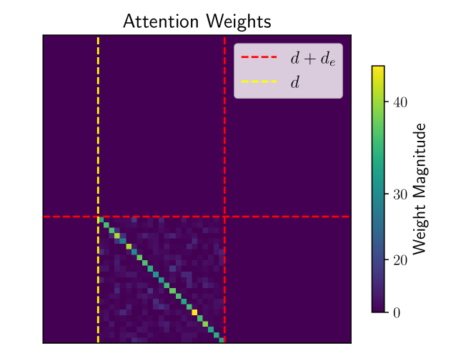
Figure 2: The trained attention weights $\boldsymbol{W}_{Q}^{\top}\boldsymbol{W}_{K}$ match our theoretical construction, see Equation (A.2). We use the $1\mathrm{STR}$ setup of Figure 1 with $N=100$.

We make the following remarks.

• First, the sample complexity above depends on $N$ only up to log factors as desired. Second, we can remove the $C_{1}$ factor by performing a clipping operation with a sufficiently large constant on the Transformer output. Note that the first and second terms in the RHS above denote the approximation and estimation errors respectively. Extending the above guarantee to cover $m\geq m_{g}$ and $H\geq q$ is straightforward.

• This bound provides guidance on the relative merits of scaling the parameter complexity of the feedforward versus the attention layer, which remains an active research area related to Transformer scaling laws [24, 26], by highlighting the trade-off between the two in achieving minimal generalization error. Concretely, $m_{g}\gg d+q$ represents a regime where the complexity is dominated by the feedforward layer learning the downstream task $g$, while $m_{g}\ll d+q$ signifies dominance of the attention layer learning to retrieve the relevant tokens.

• By incorporating additional structure in the ERM solution, it is possible to obtain improved sample complexities. A close study of the optimization dynamics may reveal such additional structure in the solution reached by gradient-based methods, pushing the sample complexity closer to the information-theoretic limit of $\Omega(qd)$. Figure 2 demonstrates that the attention weights achieved through standard optimization of a Transformer match our theoretical constructions (see Equation A.2), even while maintaining separate $\boldsymbol{W}_{Q}$ and $\boldsymbol{W}_{K}$ during training. We leave the study of optimization dynamics and the resulting sample complexity for future work.

4 Feedforward Neural Networks (FFNs)

In this section, we consider a general formulation of a feedforward network. Our only requirement will be that the first layer performs a fully-connected projection. The subsequent layers of the network can be arbitrarily implemented, e.g. using attention blocks or convolution filters. Specifically, the FFN will implement the mapping $\boldsymbol{p}\mapsto f(\boldsymbol{T},\boldsymbol{W}\boldsymbol{x})$ where $\boldsymbol{W}\in\mathbb{R}^{m_{1}\times Nd}$ is the weight matrix in the first layer, $\boldsymbol{x}=(\boldsymbol{x}_{1}^{\top},\ldots,\boldsymbol{x}_{N}^{\top})^{\top}\in\mathbb{R}^{Nd}$, and $f:[N]^{qN}\times\mathbb{R}^{m_{1}}\to\mathbb{R}^{N}$ implements the rest of the network. Unlike the Transformer architecture, here we give the network full information of $\boldsymbol{T}=(\boldsymbol{t}_{1},\ldots,\boldsymbol{t}_{N})$, and in particular the network can implement arbitrary encodings of the position variables $\boldsymbol{t}_{1},\ldots,\boldsymbol{t}_{N}$. This formulation covers usual approaches where encodings of $\boldsymbol{t}$ are added to or concatenated with $\boldsymbol{x}$.

For our negative result on feedforward networks, we can further restrict the class of $q\mathrm{STR}$ models, and only look at simple models, where a single set of indices $\boldsymbol{t}$ is shared at all positions. Note that for simple-$q\mathrm{STR}$ models, $\hat{R}_{n}$ of (2.3) and $\hat{R}_{n,N}$ of (2.2) will be equivalent, thus we only consider one of them. Additionally, the lower bound of this section holds regardless of the loss function used for training. Therefore, for some arbitrary loss $\ell:\mathbb{R}\times\mathbb{R}\to\mathbb{R}$, we define the empirical risk of the FFN as

$$\hat{\mathcal{L}}^{{\texttt{FFN}}}(f,\boldsymbol{W})\coloneqq\frac{1}{nN}\sum_{i=1}^{n}\sum_{j=1}^{N}\ell(y^{(i)}_{j},f(\boldsymbol{T}^{(i)},\boldsymbol{W}\boldsymbol{x}^{(i)})_{j}),$$

where $\boldsymbol{T}^{(i)}=(\boldsymbol{t}^{(i)}_{1},\ldots,\boldsymbol{t}^{(i)}_{N})$. We still use $R^{\texttt{FFN}}(f,\boldsymbol{W})$ for expected squared loss. Our lower bound covers a broad set of algorithms, characterized by the following definition.

Definition 5.

Let $\mathcal{A}_{\mathrm{SP}}$ denote the set of algorithms that return a stationary point of the regularized empirical risk of an FFN. Specifically, for every $A\in\mathcal{A}$, $A(S_{n})$ returns $f_{A(S_{n})}$ and $\boldsymbol{W}_{A(S_{n})}$, such that

$$\nabla_{\boldsymbol{W}}\hat{\mathcal{L}}^{{\texttt{FFN}}}(f_{A(S_{n})},\boldsymbol{W}_{A(S_{n})})+\lambda\boldsymbol{W}_{A(S_{n})}=0,$$

for some $\lambda>0$ depending on $A$. $S_{n}$ above denotes the training set. Let $\mathcal{A}_{\mathrm{ERM}}$ denote the set of algorithms that return the min-norm approximate ERM. Specifically, every $A\in\mathcal{A}_{\mathrm{ERM}}$ returns

$$A(S_{n})=\operatorname*{arg\,min}_{\{f,\boldsymbol{W}:\hat{\mathcal{L}}^{{\texttt{FFN}}}(f,\boldsymbol{W})\leq\varepsilon\}}\mathopen{}\mathclose{{\left\|{\boldsymbol{W}}}}\right\|_{\mathrm{F}},$$

for some $\varepsilon\geq 0$. Define $\mathcal{A}\coloneqq\mathcal{A}_{\mathrm{SP}}\cup\mathcal{A}_{\mathrm{ERM}}$.

In particular, $\mathcal{A}$ goes beyond constrained ERM in that it also includes the (ideal) output of first-order optimization algorithms with weight decay, or ERM with additional $\ell_{2}$ penalty on the weights. The following minimax lower bound shows that all algorithms in class $\mathcal{A}$ fail to learn even the subset of simple-$q\mathrm{STR}$ models with a sample complexity sublinear in $N$.

Theorem 6.

Suppose $\boldsymbol{x}\sim\mathcal{N}(0,\mathbf{I}_{Nd})$, and consider the simple-$1\mathrm{STR}$ model with $t_{i1}=t_{1}$ for all $i\in[N]$, where $t_{1}$ is drawn independently and uniformly in $[N]$, and a linear link function, i.e. $y=\mathopen{}\mathclose{{\left\langle{\boldsymbol{u}},{\boldsymbol{x}_{t_{1}}}}}\right\rangle$ for some $\boldsymbol{u}\in\mathbb{S}^{d-1}$. Let $\mathcal{A}$ be the class of algorithms in Definition 5. Then,

$$\inf_{A\in\mathcal{A}}\sup_{\boldsymbol{u}\in\mathbb{S}^{d-1}}R^{\texttt{FFN}}(f_{A(S_{n})},\boldsymbol{W}_{A(S_{n})})\geq 1-\frac{n}{Nd},$$

with probability $1$ over the training set $S_{n}$.

Remark. The above lower bound implies that learning the simple $1\mathrm{STR}$ model with FFNs requires at least $Nd$ samples. Note that here we do not have any assumption on $m_{1}$, i.e. the network can have infinite width. This is a crucial difference with the lower bounds in [44, 55], where the authors only prove a computational lower bound, i.e. arguing that a similar model cannot be learned unless $m_{1}\geq Nd$.

The main intuition is that from the stationarity property of Definition 5, the rows of the trained $\boldsymbol{W}$ will always be in the span of the training samples $\boldsymbol{x}^{(i)}$ for $i\in[n]$. This is an $n$-dimensional subspace, and the best predictor that only depends on this subspace still has a loss determined by the variance of $y$ conditioned on this subspace. By randomizing the target direction $\boldsymbol{u}$, we can observe that the label $y$ can depend on all $Nd$ target directions. As a result, as long as $n<Nd$, this variance will be bounded away from zero, leading to the failure of FFNs, even with infinite compute/width. For the detailed proof, we refer to Appendix B.

5 Recurrent Neural Networks

In this section, we first provide positive results for RNNs by proving that they can learn simple-$q\mathrm{STR}$ with a sample complexity only polylogarithmic in $N$, thus establishing a separation in their learning capability from feedforward networks. Next, we turn to general $q\mathrm{STR}$, where we provide a negative result on RNNs, proving that to learn such models their sample complexity must scale with $N^{\Omega(1)}$ regardless of model size, making them less statistically efficient than Transformers. Throughout this section, we focus on bidirectional RNNs, since the $q\mathrm{STR}$ model is not necessarily causal and the output at position $i$ may depend on future tokens.

5.1 RNNs can learn simple-$q\mathrm{STR}$

A bidirectional RNN maintains, for each position in the sequence, a forward and a reverse hidden state, denoted by $(\boldsymbol{h}^{\rightarrow}_{i})_{i=1}^{N}$ and $(\boldsymbol{h}^{\leftarrow}_{i})_{i=1}^{N}$, where $\boldsymbol{h}^{\rightarrow}_{i},\boldsymbol{h}^{\leftarrow}_{i}\in\mathbb{R}^{d_{h}}$. These hidden states are obtained by initializing $\boldsymbol{h}^{\rightarrow}_{1}=\boldsymbol{h}^{\leftarrow}_{N}=\boldsymbol{0}_{d_{h}}$ and recursively applying

$$\boldsymbol{h}^{\rightarrow}_{i} =\Pi_{r_{h}}\big{(}\boldsymbol{h}^{\rightarrow}_{i-1}+f^{\rightarrow}_{h}(\boldsymbol{h}^{\rightarrow}_{i-1},\boldsymbol{z}_{i-1};\boldsymbol{\Theta}^{\rightarrow}_{h})\big{)},\quad\forall i\in\{2,\ldots,N\}$$

$$\boldsymbol{h}^{\leftarrow}_{i} =\Pi_{r_{h}}\big{(}\boldsymbol{h}^{\leftarrow}_{i+1}+f^{\leftarrow}_{h}(\boldsymbol{h}^{\leftarrow}_{i+1},\boldsymbol{z}_{i+1};\boldsymbol{\Theta}^{\leftarrow}_{h})\big{)},\quad\forall i\in\{1,\ldots,N-1\},$$

where $\Pi_{r_{h}}:\mathbb{R}^{d_{h}}\to\mathbb{R}^{d_{h}}$ is the projection $\Pi_{r_{h}}\boldsymbol{h}=(1\wedge r_{h}/\mathopen{}\mathclose{{\left\|{\boldsymbol{h}}}}\right\|_{2})\boldsymbol{h}$, and $f^{\rightarrow}_{h}$ and $f^{\leftarrow}_{h}$ are implemented by feedforward networks, parameterized by $\boldsymbol{\Theta}^{\rightarrow}_{h}$ and $\boldsymbol{\Theta}^{\leftarrow}_{h}$ respectively. Recall $\boldsymbol{z}_{i}=(\boldsymbol{x}_{i}^{\top},\operatorname{enc}(i,\boldsymbol{t}_{i})^{\top})^{\top}$ is the encoding of $\boldsymbol{x}_{i}$. We remark that while we add $\Pi_{r_{h}}$ for technical reasons, it resembles layer normalization which ensures stability of the state transitions on very long inputs; a more involved analysis can replace $\Pi_{r_{h}}$ with standard formulations of layer normalization. Additionally, directly adding $\boldsymbol{h}^{\rightarrow}_{i-1}$ and $\boldsymbol{h}^{\leftarrow}_{i+1}$ to the output of transition functions represents residual or skip connections. The output at position $i$ is generated by

$$y_{i}=f_{y}(\boldsymbol{h}^{\rightarrow}_{i},\boldsymbol{h}^{\leftarrow}_{i},\boldsymbol{z}_{i};\boldsymbol{\Theta}_{y}),$$

which is another feedforward network. Specifically, we consider an RNN with deep transitions [41] and let $f^{\rightarrow}_{h}(\cdot;\boldsymbol{\Theta}^{\rightarrow}_{h})$ be an $L_{h}$ layer feedforward network, given by

$$f^{\rightarrow}_{h}(\cdot;\boldsymbol{\Theta}^{\rightarrow}_{h})=\boldsymbol{W}^{\rightarrow}_{L_{h}}\sigma\big{(}\boldsymbol{W}^{\rightarrow}_{L_{h}-1}\ldots\sigma(\boldsymbol{W}^{\rightarrow}_{2}\sigma(\boldsymbol{W}^{\rightarrow}_{1}(\cdot)+\boldsymbol{b}^{\rightarrow}_{1})+\boldsymbol{b}^{\rightarrow}_{2})\ldots+\boldsymbol{b}^{\rightarrow}_{L_{h}-1}\big{)},$$

therefore $\boldsymbol{\Theta}^{\rightarrow}_{h}=(\boldsymbol{W}^{\rightarrow}_{1},\boldsymbol{b}^{\rightarrow}_{1},\ldots,\boldsymbol{W}^{\rightarrow}_{L_{h}-1},\boldsymbol{b}^{\rightarrow}_{L_{h}-1},\boldsymbol{W}^{\rightarrow}_{L_{h}})$. We can similarly define $f^{\leftarrow}_{h}(\cdot;\boldsymbol{\Theta}^{\leftarrow}_{h})$ with depth $L_{h}$, and $f_{y}(\cdot;\boldsymbol{\Theta}_{y})$ with depth $L_{y}$. We denote the complete output of the RNN via

$$\hat{\boldsymbol{y}}_{\texttt{RNN}}(\boldsymbol{p};\boldsymbol{\Theta}_{\texttt{RNN}})=(f_{y}(\boldsymbol{h}^{\rightarrow}_{1},\boldsymbol{h}^{\leftarrow}_{1},\boldsymbol{z}_{1};\boldsymbol{\Theta}_{y}),\ldots,f_{y}(\boldsymbol{h}^{\rightarrow}_{N},\boldsymbol{h}^{\leftarrow}_{N},\boldsymbol{z}_{N};\boldsymbol{\Theta}_{y}))\in\mathbb{R}^{N}.$$

We now define the constraint set of this architecture. Let

$$\varTheta_{\texttt{RNN}}=\Big{\{}\boldsymbol{\Theta}\,:\,\mathopen{}\mathclose{{\left\|{\operatorname{vec}(\boldsymbol{\Theta})}}}\right\|_{2}\leq R,\mathopen{}\mathclose{{\left\|{\boldsymbol{W}^{\rightarrow}_{L_{h}}}}}\right\|_{\mathrm{op}}\ldots\mathopen{}\mathclose{{\left\|{\boldsymbol{W}^{\rightarrow}_{1,h}}}}\right\|_{\mathrm{op}}\leq\alpha_{N},\mathopen{}\mathclose{{\left\|{\boldsymbol{W}^{\leftarrow}_{L_{h}}}}}\right\|_{\mathrm{op}}\ldots\mathopen{}\mathclose{{\left\|{\boldsymbol{W}^{\leftarrow}_{1,h}}}}\right\|_{\mathrm{op}}\leq\alpha_{N}\Big{\}},$$

where $\boldsymbol{W}^{\rightarrow}_{1,h}$ contains the first $d_{h}$ columns of $\boldsymbol{W}^{\rightarrow}_{1}$, and the conditions above are introduced to ensure $f^{\rightarrow}_{h}$ and $f^{\leftarrow}_{h}$ are at most $\alpha_{N}$-Lipschitz with respect to the hidden state input. One way to meet this requirement is to multiply $\boldsymbol{W}^{\rightarrow}_{1,h}$ by a factor of $\alpha_{N}/\prod_{l=2}^{L_{h}}\mathopen{}\mathclose{{\left\|{\boldsymbol{W}^{\rightarrow}_{l}}}}\right\|_{\mathrm{op}}$ in the forward pass. Without this Lipschitzness constraint, current techniques for proving uniform RNN generalization bounds will suffer from a sample complexity linear in $N$, see e.g. [15]. We have the following guarantee for RNNs learning simple-$q\mathrm{STR}$ models.

Theorem 7.

Let $\hat{\boldsymbol{\Theta}}=\operatorname*{arg\,min}_{\boldsymbol{\Theta}\in\varTheta_{\texttt{RNN}}}\hat{R}^{\texttt{RNN}}_{n}(\boldsymbol{\Theta})$. Suppose Assumptions 1, 2 and 3 hold with the simple-$q\mathrm{STR}$ model, i.e. $\boldsymbol{t}_{i}=\boldsymbol{t}$ for all $i\in[N]$ and some $\boldsymbol{t}$ drawn from $[N]^{q}$. Then, with $L_{h},L_{y}=\mathcal{O}(1)$, $r_{h}=\tilde{\Theta}(\sqrt{qd})$, and for any $\alpha_{N}\leq N^{-1}$, we obtain

$$R^{\texttt{RNN}}(\hat{\boldsymbol{\Theta}})\lesssim\varepsilon_{\texttt{2NN}}+\sqrt{\frac{\operatorname{poly}(d,q,m_{g},r_{a},r_{w},\varepsilon_{\texttt{2NN}}^{-1},\log(nN))}{n}},$$

with probability at least $1-n^{-c}$ for some absolute constant $c>0$.

As desired, the above sample complexity depends on $N$ only up to polylogarithmic factors. In particular, we can choose $\alpha_{N}=0$ and fix $\boldsymbol{W}^{\rightarrow}_{1,h}=\boldsymbol{W}^{\leftarrow}_{1,h}=\boldsymbol{0}$, which would simplify the network parametrization. Namely, in our construction $f^{\rightarrow}$ and $f^{\leftarrow}$ do not need to depend on $\boldsymbol{h}^{\rightarrow}$ and $\boldsymbol{h}^{\leftarrow}$ respectively. The dimension of RNN weights, implicit in the formulation above, must have a similar polynomial scaling as evident by the proof of the above theorem in Appendix C.

5.2 RNNs cannot learn general $q\mathrm{STR}$

For our lower bound, we will consider a broad class of recurrent networks, without restricting to a specific form of parametrization. Specifically, we consider bidirectional RNNs chracterized by

$$\boldsymbol{h}^{\rightarrow}_{i+1} ={\mathrm{proj}}_{r_{h}}\big{(}f^{\rightarrow}_{h}(\boldsymbol{h}^{\rightarrow}_{i},\boldsymbol{x}_{i},\boldsymbol{t}_{i},i)\big{)},\quad\forall\,i\in\{1,\ldots,N-1\}$$

$$\boldsymbol{h}^{\leftarrow}_{i-1} ={\mathrm{proj}}_{r_{h}}\big{(}f^{\leftarrow}_{h}(\boldsymbol{h}^{\leftarrow}_{i},\boldsymbol{x}_{i},\boldsymbol{t}_{i},i)\big{)},\quad\forall\,i\in\{2,\ldots,N\}$$

$$y_{i} =f_{y}(\boldsymbol{U}^{\rightarrow}\boldsymbol{h}^{\rightarrow}_{i},\boldsymbol{U}^{\leftarrow}\boldsymbol{h}^{\leftarrow}_{i},\boldsymbol{x}_{i},\boldsymbol{t}_{i},i),\quad\forall i\in[N]$$

where $f_{y}:\mathbb{R}^{d_{h}}\times\mathbb{R}^{d_{h}}\times\mathbb{R}^{d}\times[N]^{q+1}\to\mathbb{R}$, $f^{\rightarrow}_{h},f^{\leftarrow}_{h}:\mathbb{R}^{d_{h}}\times\mathbb{R}^{d}\times[N]^{q+1}\to\mathbb{R}^{d_{h}}$, $\boldsymbol{U}^{\rightarrow},\boldsymbol{U}^{\leftarrow}\in\mathbb{R}^{d_{h}\times d_{h}}$, $d_{h}$ is the width of the model, and $r_{h}>0$ is some constant. Moreover, ${\mathrm{proj}}_{r_{h}}:\mathbb{R}^{d_{h}}\to\mathbb{R}^{d_{h}}$ is any mapping that guarantees $\mathopen{}\mathclose{{\left\|{{\mathrm{proj}}_{r_{h}}(\cdot)}}}\right\|_{2}\leq r_{h}$. As mentioned before, this operation mirrors the layer normalization to ensure that $\boldsymbol{h}_{i}$ remains stable. Further, we assume $f_{y}(\cdot,\boldsymbol{x},\boldsymbol{t})$ is $\mathfrak{L}/r_{h}$-Lipschitz for all $\boldsymbol{x}\in\mathbb{R}^{d}$ and $\boldsymbol{t}\in[N]^{q}$. This formulation covers different variants of (bidirectional) RNNs used in practice such as LSTM and GRU, and includes the RNN formulation of Section 5.1 as a special case. Define $\boldsymbol{U}\coloneqq(\boldsymbol{U}^{\rightarrow},\boldsymbol{U}^{\leftarrow})\in\mathbb{R}^{d_{h}\times 2d_{h}}$ for conciseness. Note that in practice $f_{y},f^{\rightarrow}_{h},f^{\leftarrow}_{h}$ are determined by additional parameters. However, the only weight that we explicitly denote in this formulation is $\boldsymbol{U}$, since our lower bound will directly involve this projection, and we keep the rest of the parameters implicit for our representational lower bound.

Our technique for proving a lower bound for RNNs differs significantly from that of FFNs, and in particular we will control the representation cost of the $q\mathrm{STR}$ model, i.e., a lower bound on the norm of $\boldsymbol{\Theta}_{{\texttt{RNN}}}$.

We will now present the RNN lower bound, with its proof deferred to Appendix C.3.

Proposition 8.

Consider the $1\mathrm{STR}$ model where $\boldsymbol{x}\sim\mathcal{N}(0,\mathbf{I}_{Nd})$ with a linear link function, i.e. $y_{j}=\mathopen{}\mathclose{{\left\langle{\boldsymbol{u}},{\boldsymbol{x}_{t_{j}}}}}\right\rangle$ for some $\boldsymbol{u}\in\mathbb{S}^{d-1}$. Further, $t_{i}$ is drawn independently from the rest of the prompt and uniformly from $[N]$ for all $i\in[N]$. Then, there exists an absolute constant $c>0$, such that

$$\frac{1}{N}\operatorname{\mathbb{E}}\mathopen{}\mathclose{{\left[{\mathopen{}\mathclose{{\left\|{\boldsymbol{y}-\hat{\boldsymbol{y}}_{{\texttt{RNN}}}(\boldsymbol{p})}}}\right\|^{2}}}}\right]\leq c,$$

implies

$$d_{h}\geq\Omega\Big{(}\frac{N}{\log(1+\mathfrak{L}^{2}\mathopen{}\mathclose{{\left\|{\boldsymbol{U}}}}\right\|_{\mathrm{op}}^{2})}\Big{)},\quad\text{and}\quad\mathopen{}\mathclose{{\left\|{\boldsymbol{U}}}}\right\|_{\mathrm{op}}^{2}\geq\Omega\Big{(}\frac{N}{\mathfrak{L}^{2}\log(1+d_{h})}\Big{)}.$$

Remark. Note that the unboundedness of Gaussian random variables is not an issue for approximation here, since $(g(\boldsymbol{x}_{1}),\ldots,g(\boldsymbol{x}_{N}))$ is highly concentrated around $\mathbb{S}^{N-1}(\sqrt{N})$. In fact, one can directly assume $(g(\boldsymbol{x}_{1}),\ldots,g(\boldsymbol{x}_{N}))\sim\textnormal{Unif}(\mathbb{S}^{N-1}(\sqrt{N}))$ and derive a similar lower bound. The choice of Gaussian above is only made to simplify the presentation of the proof.

The above proposition has two implications. First, it has a computational consequence, implying that any RNN representing the $q\mathrm{STR}$ models requires a width that grows at least linearly with the context-length $N$. A similar lower bound in terms of bit complexity was derived in [44] using different tools. More importantly, the norm lower bound $\mathopen{}\mathclose{{\left\|{\boldsymbol{U}}}}\right\|_{\mathrm{F}}\geq\tilde{\Omega}(\sqrt{N})$ has a generalization consequence, as it suggests that norm-based generalization bounds cannot guarantee a sample-complexity independent of $N$.

To translate the above representational cost result to a sample complexity lower bound, we now introduce the parametrization of the output function $f_{y}$. The exact parametrization of the transition functions will be unimportant, and we will use the notation $f^{\rightarrow}_{h}(\boldsymbol{h},\boldsymbol{x},\boldsymbol{t};\boldsymbol{\Theta}^{\rightarrow}_{h})$ to denote a general parameterized function (similarly with $f^{\leftarrow}$). We will assume $f_{y}$ is given by a feedforward network,

$$f_{y}(\boldsymbol{U}^{\rightarrow}\boldsymbol{h}^{\rightarrow},\boldsymbol{U}^{\leftarrow}\boldsymbol{h}^{\leftarrow},\boldsymbol{x},\boldsymbol{t};\boldsymbol{\Theta}_{y})=\boldsymbol{W}_{L_{y}}\sigma\big{(}\ldots\sigma(\boldsymbol{W}_{2}\sigma(\boldsymbol{U}\boldsymbol{h}+\boldsymbol{W}_{y}\boldsymbol{z}+\boldsymbol{b}_{y})+\boldsymbol{b}_{2})\ldots\big{)},$$

where $\boldsymbol{h}=(\boldsymbol{h}^{\rightarrow},\boldsymbol{h}^{\leftarrow})\in\mathbb{R}^{2d_{h}}$, $\boldsymbol{z}=(\boldsymbol{x}_{i},f_{E}(\boldsymbol{t}_{i},i))\in\mathbb{R}^{d+d_{E}}$. Here, $f_{E}(\boldsymbol{t}_{i},i)$ is an arbitrary encoding function with arbitrary dimension $d_{E}$. Then $\boldsymbol{\Theta}_{y}=(\boldsymbol{U},\boldsymbol{W}_{y},\boldsymbol{b}_{y},\boldsymbol{W}_{2},\boldsymbol{b}_{2},\ldots,\boldsymbol{W}_{L_{y}})$, and $\boldsymbol{\Theta}_{\texttt{RNN}}=(\boldsymbol{U},\boldsymbol{\Theta}_{y},\boldsymbol{\Theta}^{\rightarrow}_{h},\boldsymbol{\Theta}^{\leftarrow}_{h})$. Note that thanks to the homogeneity of ReLU, we can always reparameterize the network by taking $\bar{\boldsymbol{h}}=\boldsymbol{h}/r_{h}$, $\bar{\boldsymbol{W}}_{y}=\boldsymbol{W}_{y}/r_{h}$, $\bar{\boldsymbol{b}}_{y}=\boldsymbol{b}_{y}/r_{h}$, and $\bar{\boldsymbol{W}}_{2}=\boldsymbol{W}_{2}/r_{h}$ without changing the prediction function. Thus, in the following, we take $r_{h}=1$ without losing the expressive power of the network. We then have the following lower bound on the sample complexity of min-norm $\varepsilon$-ERM.

Theorem 9.

Consider the $1\mathrm{STR}$ model of Proposition 8. Suppose the size of the hidden state, the depth of the prediction function, and the weight norm respectively satisfy $d_{h}\leq e^{N^{c}}$, $2\leq L_{y}\leq C$, and $\mathopen{}\mathclose{{\left\|{\operatorname{vec}(\boldsymbol{\Theta}_{\texttt{RNN}})}}}\right\|_{2}\leq e^{N^{c}/L_{y}}$ for some absolute constants $c<1$ and $C\geq 2$, and recall we set $r_{h}=1$ due to homogeneity of the network. Let $\hat{\boldsymbol{\Theta}}_{\varepsilon}$ be the min-norm $\varepsilon$-ERM of $\hat{R}^{\texttt{RNN}}_{n}$, defined in (2.4). Then, there exist absolute constants $c_{1},c_{2},c_{3}>0$ such that if $n\leq\mathcal{O}(N^{c_{1}})$, for any $\varepsilon\geq 0$, with probability at least $c_{2}$ over the training set,

$$\frac{1}{N}\operatorname{\mathbb{E}}\mathopen{}\mathclose{{\left[{\mathopen{}\mathclose{{\left\|{\hat{\boldsymbol{y}}_{\texttt{RNN}}(\boldsymbol{p};\hat{\boldsymbol{\Theta}}_{n,\varepsilon})-\boldsymbol{y}}}}\right\|_{2}^{2}}}}\right]\geq c_{3}.$$

Remark. It is possible to remove the subexponential bound on $\mathopen{}\mathclose{{\left\|{\operatorname{vec}(\boldsymbol{\Theta}_{\texttt{RNN}})}}}\right\|$ by allowing the learner to search over families of RNN architectures with arbitrary $d_{h}\leq e^{N^{c}}$ rather than fixing a single $d_{h}$. In practice, even when fixing $d_{h}$, one would avoid solutions that violate this norm constraint due to numerical instability.

To prove the above theorem, we use the fact that an RNN that generalizes on the entire data distribution (hence approximates the $1\mathrm{STR}$ model) requires a weight norm that scales with $\sqrt{N}$, while overfitting on the $n$ samples in the training set with zero empirical risk is possible with a $\operatorname{poly}(n)$ weight norm. As a result, as long as $n\leq N^{c_{1}}$ for some small constant $c_{1}>0$, min-norm $\varepsilon$-ERM will choose models that overfit rather than generalize. A similar approach was taken in [42] to prove sample complexity separations between two and three-layer feedforward networks. The complete proof is presented in Appendix C.4.

6 Conclusion

In this paper, we established a sample complexity separation between Transformers and baseline architectures, namely feedforward and recurrent networks, for learning sequence-to-sequence models where the output at each position depends on a sparse subset of input tokens described in the input itself, coined the $q\mathrm{STR}$ model. We proved that Transformers can learn such a model with sample complexity almost independent of the length of the input sequence $N$, while feedforward and recurrent networks have sample complexity lower bounds of $N$ and $N^{\Omega(1)}$, respectively. Further, we established a separation between FFNs and RNNs by proving that recurrent networks can learn the subset of simple-$q\mathrm{STR}$ models where the output at all positions is identical, whereas feedforward networks require at least $N$ samples. An important direction for future work is to develop an understanding of the optimization dynamics of Transformers to learn $q\mathrm{STR}$ models, and to study sample complexity separations that highlight the role of depth in Transformers.

Appendix A Details of Section 3

Here we present the omitted results and proofs of Section 3. We begin by presenting the improved sample complexity for Transformers.

A.1 Proof of Theorem 4

To prove Theorem 4, we will prove the more general theorem below.

Theorem 10.

Let $\hat{\boldsymbol{\Theta}}\coloneqq\operatorname*{arg\,min}_{\boldsymbol{\Theta}\in\varTheta_{{\texttt{TR}}}}\hat{R}^{\texttt{TR}}_{n}(\boldsymbol{\Theta})$, where

$$\varTheta_{{\texttt{TR}}}\coloneqq\Big{\{} \mathopen{}\mathclose{{\left\|{\boldsymbol{a}_{\texttt{2NN}}}}}\right\|_{2}\leq r_{a}/\sqrt{m},\mathopen{}\mathclose{{\left\|{(\boldsymbol{W}_{{\texttt{2NN}}},\boldsymbol{b}_{\texttt{2NN}})}}}\right\|_{\mathrm{F}}\leq r_{w}\sqrt{m},\mathopen{}\mathclose{{\left\|{\boldsymbol{W}^{(h)}_{\mathrm{QK}}}}}\right\|_{2,1}\leq\alpha\,\,\forall h\in[H]\Big{\}}.$$

Suppose $H=q$, $m=m_{g}$, and $\alpha=\tilde{\Theta}(1)$ (given in Lemma 11). Then, under Assumptions 1, 2 and 3, with probability at least $1-n^{-c}$ for some absolute constant $c>0$, we have

$$R^{\texttt{TR}}(\hat{\boldsymbol{\Theta}})\leq\mathcal{O}(\varepsilon_{\mathrm{NN}}^{2})+\tilde{\mathcal{O}}\mathopen{}\mathclose{{\left(C_{1}\sqrt{\frac{(m_{g}q(d+q)+r_{z}^{6}r_{a}^{2}r_{w}^{2}q^{2}\wedge q(q^{2}+d^{2}))}{n}}}}\right),$$ (A.1)

where $C_{1}=qr_{a}^{2}r_{w}^{2}r_{z}^{2}$.

We begin with a lemma establishing the capability of Transformers in approximating $q\mathrm{STR}$ models.

Lemma 11.

Suppose Assumption 2 holds. Let $r_{x}=\sqrt{3C_{x}ed\log(nN)}$. Assume $H=q$ and $m_{g}=m$. Then, there exists $\boldsymbol{\Theta}_{\texttt{TR}}$ such that

$$\sup_{\{\mathopen{}\mathclose{{\left\|{\boldsymbol{x}_{j}}}}\right\|_{2}\leq r_{x},\,\forall j\in[N]\}}\mathopen{}\mathclose{{\left|g(\boldsymbol{x}_{t_{i1}},\ldots,\boldsymbol{x}_{t_{iq}})-\hat{y}_{\texttt{TR}}(\boldsymbol{p};\boldsymbol{\Theta}_{\texttt{TR}})_{i}}}\right|\leq 2\sqrt{\varepsilon_{\texttt{2NN}}},$$

and

$$\mathopen{}\mathclose{{\left\|{\boldsymbol{a}_{\texttt{2NN}}}}}\right\|_{2}\leq\frac{r_{a}}{\sqrt{m}},\quad\mathopen{}\mathclose{{\left\|{(\boldsymbol{W}_{\texttt{2NN}},\boldsymbol{b}_{\texttt{2NN}})}}}\right\|_{\mathrm{F}}\leq\sqrt{m}r_{w},\quad{\mathopen{}\mathclose{{\left\|{{\boldsymbol{W}^{(h)}_{\mathrm{QK}}}^{\top}}}}\right\|}_{2,1}\leq\frac{2d_{e}q}{d}\log\mathopen{}\mathclose{{\left(\frac{2r_{a}r_{w}r_{x}N\sqrt{q}}{\varepsilon_{\texttt{2NN}}}}}\right),$$

for all $h\in[H]$.

Proof.  In our construction, the goal of attention head $h$ at position $i$ will be to output $z_{t_{ih}}$. Namely, we want to achieve

$$f_{\texttt{Attn}}(\boldsymbol{p};\boldsymbol{W}^{(h)}_{\mathrm{QK}})_{i}\approx\boldsymbol{z}_{t_{ih}}.$$

Note that to do so, for each key token $\boldsymbol{z}_{j}$, we only need to compute $\mathopen{}\mathclose{{\left\langle{\boldsymbol{\omega}_{t_{ih}}},{\boldsymbol{\omega}_{j}}}}\right\rangle$. Therefore, most entries in $\boldsymbol{W}^{(h)}_{\mathrm{QK}}$ can be zero. We only require a block of $d_{e}\times d_{e}$, which corresponds to comparing $\boldsymbol{\omega}_{j}$ and $\boldsymbol{\omega}_{t_{ih}}$ when comparing query $\boldsymbol{z}_{i}$ and key $\boldsymbol{z}_{j}$. Thus, we let

$$\boldsymbol{W}^{(h)}_{\mathrm{QK}}=\begin{pmatrix}\boldsymbol{0}_{(d+hd_{e})\times d}&\boldsymbol{0}_{(d+hd_{e})\times d_{e}}&\boldsymbol{0}_{(d+hd_{e})\times qd_{e}}\\ \boldsymbol{0}_{d_{e}\times d}&\alpha\mathbf{I}_{d_{e}}&\boldsymbol{0}_{d_{e}\times qd_{e}}\\ \boldsymbol{0}_{(q-h)d_{e}\times d}&\boldsymbol{0}_{(q-h)d_{e}\times d_{e}}&\boldsymbol{0}_{(q-h)d_{e}\times qd_{e}}\end{pmatrix}$$ (A.2)

Then, we have $\mathopen{}\mathclose{{\left\langle{\boldsymbol{z}_{i}},{\boldsymbol{W}^{(h)}_{\mathrm{QK}}\boldsymbol{z}_{j}}}}\right\rangle=\alpha\mathopen{}\mathclose{{\left\langle{\boldsymbol{\omega}_{t_{ih}}},{\boldsymbol{\omega}_{j}}}}\right\rangle d/q$. We can then verify that

$$\mathopen{}\mathclose{{\left\|{\boldsymbol{A}f_{\texttt{Attn}}(\boldsymbol{p};\boldsymbol{W}^{(h)}_{\mathrm{QK}})_{i}-\boldsymbol{A}\boldsymbol{z}_{t_{ih}}}}}\right\|_{2} \leq\sum_{j\neq t_{ih}}e^{-\alpha d/(2q)}(\mathopen{}\mathclose{{\left\|{\boldsymbol{A}\boldsymbol{z}_{j}}}}\right\|+\mathopen{}\mathclose{{\left\|{\boldsymbol{A}\boldsymbol{z}_{t_{ih}}}}}\right\|_{2})$$

for every matrix $\boldsymbol{A}$. We will specifically choose $\boldsymbol{A}$ to be the projection onto the first $d$ coordinates in the following. Hence, $\alpha$ will control the error in the softmax attention approximating a “hard-max” attention that would exactly choose $\boldsymbol{z}_{t_{ih}}$.

To construct the weights of the feedforward layer $\boldsymbol{a}_{\texttt{2NN}},\boldsymbol{W}_{\texttt{2NN}},\boldsymbol{b}_{\texttt{2NN}}$, we let $\boldsymbol{a}_{\texttt{2NN}}=\boldsymbol{a}_{g}$ and $\boldsymbol{b}_{\texttt{2NN}}=\boldsymbol{b}_{g}$ from Assumption 2, and define $\boldsymbol{W}_{\texttt{2NN}}$ by extending $\boldsymbol{W}_{g}$ with zero entries such that

$$\boldsymbol{W}_{\texttt{2NN}}\begin{pmatrix}\boldsymbol{z}_{t_{i1}}\\ \ldots\\ \boldsymbol{z}_{t_{iq}}\end{pmatrix}=\boldsymbol{W}_{g}\begin{pmatrix}\boldsymbol{x}_{t_{i1}}\\ \ldots\\ \boldsymbol{x}_{t_{iq}}\end{pmatrix}.$$

Then $\mathopen{}\mathclose{{\left\|{\boldsymbol{W}_{\texttt{2NN}}}}}\right\|_{\mathrm{F}}=\mathopen{}\mathclose{{\left\|{\boldsymbol{W}_{g}}}}\right\|_{\mathrm{F}}$. Notice that $\cdot\mapsto\boldsymbol{a}^{\top}\sigma(\boldsymbol{W}(\cdot)+\boldsymbol{b})$ is $r_{a}r_{w}$ Lipschitz. As a result, for any $\boldsymbol{x}$ with $\mathopen{}\mathclose{{\left\|{\boldsymbol{x}}}}\right\|\leq r_{x}$ we have

$$\mathopen{}\mathclose{{\left|g(\boldsymbol{x}_{t_{i1}},\ldots,\boldsymbol{x}_{t_{iq}})-\hat{y}_{{\texttt{TR}}}(\boldsymbol{p};\boldsymbol{\Theta}_{{\texttt{TR}}})_{i}}}\right|\leq\sqrt{\varepsilon_{\texttt{2NN}}}+\varepsilon_{\texttt{Attn}},$$

where we recall

$$\mathopen{}\mathclose{{\left|g(\boldsymbol{x}_{t_{i1}},\ldots,\boldsymbol{x}_{t_{iq}})-f_{\texttt{2NN}}((\boldsymbol{z}_{t_{i1}},\ldots,\boldsymbol{z}_{t_{iq}});\boldsymbol{a}_{\texttt{2NN}},\boldsymbol{W}_{\texttt{2NN}},\boldsymbol{b}_{\texttt{2NN}})}}\right|\leq\sqrt{\varepsilon_{\texttt{2NN}}},$$

and

$$\varepsilon_{\texttt{Attn}} =\mathopen{}\mathclose{{\left|f_{\texttt{2NN}}((\boldsymbol{z}_{t_{i1}},\ldots,\boldsymbol{z}_{t_{iq}});\boldsymbol{\Theta}_{\texttt{2NN}})-f_{\texttt{2NN}}(f^{(q)}_{\texttt{Attn}}(\boldsymbol{p};\boldsymbol{\Theta}_{\mathrm{QK}});\boldsymbol{\Theta}_{\texttt{2NN}})}}\right|$$

$$\leq r_{a}r_{w}\sqrt{\sum_{h=1}^{q}\mathopen{}\mathclose{{\left\|{\boldsymbol{A}f_{\texttt{Attn}}(\boldsymbol{p};\boldsymbol{W}^{(h)}_{\mathrm{QK}})_{i}-\boldsymbol{A}\boldsymbol{z}_{t_{ih}}}}}\right\|_{2}^{2}}$$

$$\leq 2r_{a}r_{w}r_{x}N\sqrt{q}e^{-\alpha d/(2q)},$$

where we recall $\boldsymbol{A}\boldsymbol{z}_{j}=\boldsymbol{x}_{j}$. Thus, with

$$\alpha=2q\log(2r_{a}r_{w}r_{x}N\sqrt{q}/\sqrt{\varepsilon_{\texttt{2NN}}})/d$$

we can guarantee the distance is at most $2\sqrt{\varepsilon_{\texttt{2NN}}}$. ∎

Before proceeding to obtain statistical guarantees, we will show that we can consider the encodings $\boldsymbol{z}^{(i)}_{j}$ to be bounded with high probability. This will be a useful event to consider throughout the proofs of various sections.

Lemma 12.

Suppose $\{\boldsymbol{p}^{(i)}\}_{i=1}^{n}$ are $n$ input prompts (not necessarily independent) drawn from the input distribution, with tokens denoted by $\{(\boldsymbol{x}^{(i)}_{j})_{j=1}^{N}\}_{i=1}^{n}$. Under Assumption 1, for any $r_{x}>0$ we have

$$\mathbb{P}\mathopen{}\mathclose{{\left({\max_{i\in[n],j\in[N]}\mathopen{}\mathclose{{\left\|{\boldsymbol{x}^{(i)}_{j}}}}\right\|_{2}\geq r_{x}}}}\right)\leq nNe^{-r_{x}^{2}/(2C_{x}ed)}.$$

In particular, for $r_{x}=\sqrt{3C_{x}ed\log(nN)}$ we have

$$\mathbb{P}\mathopen{}\mathclose{{\left({\max_{i\in[n],j\in[N]}\mathopen{}\mathclose{{\left\|{\boldsymbol{x}^{(i)}_{j}}}}\right\|_{2}\geq r_{x}}}}\right)\leq\sqrt{\frac{1}{nN}}.$$

Proof.  Via Markov’s inequality, for any $p>0$ and $r_{x}>0$, we have

$$\mathbb{P}\mathopen{}\mathclose{{\left({\max_{i,j}\mathopen{}\mathclose{{\left\|{\boldsymbol{x}^{(i)}_{j}}}}\right\|_{2}\geq r_{x}}}}\right) \leq\frac{\operatorname{\mathbb{E}}\mathopen{}\mathclose{{\left[{\max_{i,j}\mathopen{}\mathclose{{\left\|{\boldsymbol{x}^{(i)}_{j}}}}\right\|_{2}^{p}}}}\right]}{r_{x}^{p}}\leq\frac{\operatorname{\mathbb{E}}\mathopen{}\mathclose{{\left[{\sum_{i,j}\mathopen{}\mathclose{{\left\|{\boldsymbol{x}^{(i)}_{j}}}}\right\|_{2}^{p}}}}\right]}{r_{x}^{p}}\leq\frac{Nn(C_{x}pd)^{p/2}}{r^{p}_{x}}.$$

Let $p=r_{x}^{2}/(C_{x}ed)$. Then,

$$\mathbb{P}\mathopen{}\mathclose{{\left({\max_{i,j}\mathopen{}\mathclose{{\left\|{\boldsymbol{x}^{(i)}_{j}}}}\right\|_{2}\geq r_{x}}}}\right)\leq nNe^{-r_{x}^{2}/(2C_{x}ed)},$$

which proves the first statement, and the second statement follows by plugging in the specific value of $r_{x}$. ∎

We are now ready to move to the generalization analysis of Transformers. First, we have to formally define the prediction function class of Transformers with a notation suitable for this section. We begin by defining the function class of attention. We have

$$\mathcal{F}_{{\texttt{Attn}}}=\{\boldsymbol{p},j\mapsto f^{(H)}_{{\texttt{Attn}}}(\boldsymbol{p};\boldsymbol{\Theta}_{\mathrm{QK}})_{j}:\boldsymbol{\Theta}_{\mathrm{QK}}\in\varTheta_{\mathrm{QK}}\},$$

where we will later specify $\varTheta_{\mathrm{QK}}$. Additionally, we define $\mathcal{F}_{{\texttt{2NN}}}$ by

$$\mathcal{F}_{{\texttt{2NN}}}=\{\boldsymbol{h}\mapsto f_{{\texttt{2NN}}}(\boldsymbol{h};\boldsymbol{\Theta}_{\texttt{2NN}})\,:\,\boldsymbol{\Theta}_{\texttt{2NN}}\in\varTheta_{\texttt{2NN}}\},$$

where $\boldsymbol{\Theta}_{\texttt{2NN}}=(\boldsymbol{a}_{\texttt{2NN}},\boldsymbol{W}_{\texttt{2NN}},\boldsymbol{b}_{\texttt{2NN}})$, and we will later specify $\varTheta_{\texttt{2NN}}$. Then the class $\mathcal{F}_{{\texttt{TR}}}$ can be defined as

$$\mathcal{F}_{{\texttt{TR}}}=\{\boldsymbol{p},j\mapsto f_{{\texttt{2NN}}}(f_{{\texttt{Attn}}}(\boldsymbol{p})_{j})\,:\,f_{\texttt{Attn}}\in\mathcal{F}_{{\texttt{Attn}}},f_{{\texttt{2NN}}}\in\mathcal{F}_{\texttt{2NN}}\}.$$

Recall we use the $S_{n}$ to denote the training set. To avoid extra indices, we will use the notation $\boldsymbol{p},j\in S_{n}$ to go over $\{\boldsymbol{p}^{(i)},j^{(i)}\}_{i=1}^{n}$. We can then define the following distances on the introduced function classes

$$d^{\texttt{TR}}_{\infty}(f,f^{\prime}) \coloneqq\sup_{\boldsymbol{p},j}\mathopen{}\mathclose{{\left|f(\boldsymbol{p})_{j}-f^{\prime}(\boldsymbol{p})_{j}}}\right|,\quad\forall f,f^{\prime}\in\mathcal{F}_{\texttt{TR}}$$

$$d^{\texttt{Attn}}_{\infty}(f,f^{\prime}) \coloneqq\sup_{\boldsymbol{p},j}\mathopen{}\mathclose{{\left\|{f(\boldsymbol{p})_{j}-f^{\prime}(\boldsymbol{p})_{j}}}}\right\|_{2},\quad\forall f,f^{\prime}\in\mathcal{F}_{\texttt{Attn}}$$

$$d^{\texttt{2NN}}_{\infty}(f,f^{\prime}) \coloneqq\sup_{\mathopen{}\mathclose{{\left\|{\cdot}}}\right\|_{2}\leq\sqrt{H}r_{z}}\mathopen{}\mathclose{{\left|f(\cdot)-f^{\prime}(\cdot)}}\right|,\quad\forall f,f^{\prime}\in\mathcal{F}_{\texttt{2NN}}.$$

We choose the radius $\sqrt{H}r_{z}$ for defining $d^{\texttt{2NN}}_{\infty}$ since on the event of Lemma 12, this will be the norm bound on the output of the attention layer at every position.

Recall that for a distance $d_{\infty}$ and a set $\mathcal{F}$, an $\epsilon$-covering $\hat{\mathcal{F}}$ is a set such that for every $f\in\mathcal{F}$, there exists $\hat{f}\in\hat{\mathcal{F}}$ such that $d_{\infty}(f,\hat{f})\leq\epsilon$. The $\epsilon$-covering number of $\mathcal{F}$, denoted by $\mathcal{C}(\mathcal{F},d_{\infty},\epsilon)$, is the number of elements of the smallest such $\hat{\mathcal{F}}$. The following lemma relates the covering number of $\mathcal{F}_{\texttt{TR}}$ to those of $\mathcal{F}_{\texttt{Attn}}$ and $\mathcal{F}_{\texttt{2NN}}$.

Lemma 13.

Suppose $f_{{\texttt{2NN}}}$ is $L_{f}$ Lipschitz for every $f_{{\texttt{2NN}}}\in\mathcal{F}_{{\texttt{2NN}}}$. Then, for any $\epsilon_{\texttt{2NN}},\epsilon_{\texttt{Attn}}>0$, on the event of Lemma 12 we have

$$\log\mathcal{C}(\mathcal{F}_{{\texttt{TR}}},d^{\texttt{TR}}_{\infty},\epsilon_{\texttt{2NN}}+L_{f}\epsilon_{\texttt{Attn}})\leq\log\mathcal{C}\mathopen{}\mathclose{{\left(\mathcal{F}_{{\texttt{2NN}}},d^{\texttt{2NN}}_{\infty},\epsilon_{\texttt{2NN}}}}\right)+\log\mathcal{C}\mathopen{}\mathclose{{\left(\mathcal{F}_{{\texttt{Attn}}},d^{\texttt{Attn}}_{\infty},\epsilon_{\texttt{Attn}}}}\right).$$

Proof.  The proof simply follows from the triangle inequality, namely

$$\sup_{\boldsymbol{p},j}\mathopen{}\mathclose{{\left|f_{{\texttt{TR}}}(\boldsymbol{p};\boldsymbol{\Theta}_{{\texttt{TR}}})_{j}-f_{{\texttt{TR}}}(\boldsymbol{p};\hat{\boldsymbol{\Theta}}_{{\texttt{TR}}})_{j}}}\right|\leq \sup_{\mathopen{}\mathclose{{\left\|{\boldsymbol{h}}}}\right\|_{2}\leq\sqrt{H}r_{z}}\mathopen{}\mathclose{{\left\|{f_{{\texttt{2NN}}}(\boldsymbol{h};\boldsymbol{\Theta}_{\mathrm{NN}})-f_{{\texttt{2NN}}}(\boldsymbol{h};\hat{\boldsymbol{\Theta}}_{\mathrm{NN}})}}}\right\|_{2}$$

$$+L_{f}\sup_{\boldsymbol{p},j}\mathopen{}\mathclose{{\left\|{f^{(H)}_{\texttt{Attn}}(\boldsymbol{p};\boldsymbol{\Theta}_{\mathrm{QK}})_{j}-f^{(H)}_{\texttt{Attn}}(\boldsymbol{p};\hat{\boldsymbol{\Theta}}_{\mathrm{QK}})_{j}}}}\right\|_{2}.$$

∎

We have the following estimate for the covering number of $\mathcal{F}_{{\texttt{2NN}}}$.

Lemma 14.

Suppose $\mathopen{}\mathclose{{\left\|{\operatorname{vec}(\boldsymbol{\Theta}_{\texttt{RNN}})}}}\right\|_{2}\leq R$ and $\mathopen{}\mathclose{{\left\|{\boldsymbol{z}^{(i)}_{j}}}}\right\|_{2}\leq R$ for all $i\in[n]$ and $j\in[N]$. Then,

$$\log\mathcal{C}\mathopen{}\mathclose{{\left(\mathcal{F}_{{\texttt{2NN}}},d^{\texttt{2NN}}_{\infty},\epsilon}}\right)\lesssim m_{g}HD_{e}\log(1+\operatorname{poly}(R)/\epsilon).$$

This is a special case of Lemma 30, proved in Appendix C.

For the next step, define the distance

$$d^{\mathrm{QK}}_{\infty}(\boldsymbol{\Theta}_{\mathrm{QK}},\boldsymbol{\Theta}^{\prime}_{\mathrm{QK}})\coloneqq\sup_{\boldsymbol{p},j}\mathopen{}\mathclose{{\left\|{\boldsymbol{\Theta}_{\mathrm{QK}}^{\top}\boldsymbol{z}_{j}-{\boldsymbol{\Theta}^{\prime}}_{\mathrm{QK}}^{\top}\boldsymbol{z}_{j}}}}\right\|_{2}$$

on $\varTheta_{\mathrm{QK}}$, where we recall $\boldsymbol{\Theta}_{\mathrm{QK}}=(\boldsymbol{W}^{(1)}_{\mathrm{QK}},\ldots,\boldsymbol{W}^{(H)}_{\mathrm{QK}})\in\mathbb{R}^{D_{e}\times HD_{e}}$. The following lemma relates the covering number of the multi-head attention layer to the matrix covering number of the class of attention parameters.

Lemma 15.

Suppose $\mathopen{}\mathclose{{\left\|{\boldsymbol{z}^{(i)}_{j}}}}\right\|_{2}\leq r_{z}$ for all $i\in[n]$ and $j\in[N]$. Then,

$$\log\mathcal{C}(\mathcal{F}_{\texttt{Attn}},d^{\texttt{Attn}}_{\infty},\epsilon)\leq\log\mathcal{C}\mathopen{}\mathclose{{\left(\varTheta_{\mathrm{QK}},d^{\mathrm{QK}}_{\infty},\frac{\epsilon}{2r_{z}^{2}}}}\right).$$

Proof.  We recall that $\boldsymbol{Z}\in\mathbb{R}^{N\times D_{e}}$ denotes the encoded prompt, and $\operatorname{softmax}$ is applied row-wise. For conciseness, Let $\Delta\coloneqq\sup_{\boldsymbol{p},j}\mathopen{}\mathclose{{\left\|{f^{(H)}_{\texttt{Attn}}(\boldsymbol{p};\boldsymbol{\Theta}_{\mathrm{QK}})_{j}-f^{(H)}_{\texttt{Attn}}(\boldsymbol{p};\hat{\boldsymbol{\Theta}}_{\mathrm{QK}})_{j}}}}\right\|_{2}^{2}$. Then we have

$$\Delta =\sup_{\boldsymbol{p},j\in S_{n}}\sum_{h\in[H]}\mathopen{}\mathclose{{\left\|{f_{\texttt{Attn}}(\boldsymbol{p};\boldsymbol{W}^{(h)}_{\mathrm{QK}})_{j}-f_{\texttt{Attn}}(\boldsymbol{p};\hat{\boldsymbol{W}}^{(h)}_{\mathrm{QK}})_{j}}}}\right\|_{2}^{2}$$

$$=\sup_{\boldsymbol{p},j\in S_{n}}\sum_{h\in[H]}\mathopen{}\mathclose{{\left\|{\operatorname{softmax}\big{(}\boldsymbol{z}_{j}^{\top}\boldsymbol{W}_{\mathrm{QK}}^{(h)}\boldsymbol{Z}^{\top}\big{)}\boldsymbol{Z}-\operatorname{softmax}\big{(}\boldsymbol{z}_{j}^{\top}\hat{\boldsymbol{W}}_{\mathrm{QK}}^{(h)}\boldsymbol{Z}^{\top}\big{)}\boldsymbol{Z}}}}\right\|_{2}^{2}$$

$$\leq\sup_{\boldsymbol{p},j\in S_{n}}\sum_{h\in[H]}\mathopen{}\mathclose{{\left\|{\boldsymbol{Z}^{\top}}}}\right\|_{2,\infty}^{2}\mathopen{}\mathclose{{\left\|{\operatorname{softmax}(\boldsymbol{z}_{j}^{\top}\boldsymbol{W}^{(h)}_{\mathrm{QK}}\boldsymbol{Z}^{\top})^{\top}-\operatorname{softmax}(\boldsymbol{z}_{j}^{\top}\hat{\boldsymbol{W}}^{(h)}_{\mathrm{QK}}\boldsymbol{Z}^{\top})^{\top}}}}\right\|_{1}^{2},$$

where we used Lemma 39 for the last inequality. Moreover, by [20, Corollary A.7],

$$\mathopen{}\mathclose{{\left\|{\operatorname{softmax}\big{(}\boldsymbol{z}_{j}^{\top}\boldsymbol{W}^{(h)}_{\mathrm{QK}}\boldsymbol{Z}^{\top}\big{)}^{\top}-\operatorname{softmax}\big{(}\boldsymbol{z}_{j}^{\top}\hat{\boldsymbol{W}}^{(h)}_{\mathrm{QK}}\boldsymbol{Z}^{\top}\big{)}}}}\right\|_{1} \leq 2\mathopen{}\mathclose{{\left\|{\boldsymbol{Z}{\boldsymbol{W}^{(h)}}^{\top}_{\mathrm{QK}}\boldsymbol{z}_{j}-\boldsymbol{Z}{\hat{\boldsymbol{W}}^{(h)}}{}^{\top}_{\mathrm{QK}}\boldsymbol{z}_{j}}}}\right\|_{\infty}$$

$$\leq 2\mathopen{}\mathclose{{\left\|{\boldsymbol{Z}^{\top}}}}\right\|_{2,\infty}\mathopen{}\mathclose{{\left\|{{\boldsymbol{W}^{(h)}}^{\top}_{\mathrm{QK}}\boldsymbol{z}_{j}-{\hat{\boldsymbol{W}}^{(h)}}{}^{\top}_{\mathrm{QK}}\boldsymbol{z}_{j}}}}\right\|_{2}.$$

Consequently,

$$\Delta \leq 4r_{z}^{4}\sup_{\boldsymbol{p},j\in S_{n}}\sum_{h\in[H]}\mathopen{}\mathclose{{\left\|{{\boldsymbol{W}^{(h)}_{\mathrm{QK}}}^{\top}\boldsymbol{z}_{j}-{\hat{\boldsymbol{W}}^{(h)}}{}^{\top}_{\mathrm{QK}}\boldsymbol{z}_{j}}}}\right\|_{2}^{2}$$

$$=4r_{z}^{4}\sup_{\boldsymbol{p},j\in S_{n}}\mathopen{}\mathclose{{\left\|{\boldsymbol{\Theta}_{\mathrm{QK}}^{\top}\boldsymbol{z}_{j}-{\hat{\boldsymbol{\Theta}}_{\mathrm{QK}}}^{\top}\boldsymbol{z}_{j}}}}\right\|_{2}^{2},$$

which completes the proof. ∎

Further, we have the following covering number estimate for $\varTheta_{\mathrm{QK}}$.

Lemma 16.

Suppose $\varTheta_{\mathrm{QK}}=\{\mathopen{}\mathclose{{\left\|{\boldsymbol{\Theta}_{\mathrm{QK}}}}}\right\|_{2,1}\leq R_{2,1},\,\mathopen{}\mathclose{{\left\|{\boldsymbol{\Theta}_{\mathrm{QK}}}}}\right\|_{\mathrm{F}}\leq R_{F}\}$ and $\mathopen{}\mathclose{{\left\|{\boldsymbol{z}^{(i)}_{j}}}}\right\|_{2}\leq r_{z}$ for all $i\in[n]$ and $j\in[N]$. Then,

$$\log\mathcal{C}\mathopen{}\mathclose{{\left(\varTheta_{\mathrm{QK}},d^{\mathrm{QK}}_{\infty},\epsilon}}\right)\lesssim\min\mathopen{}\mathclose{{\left(\frac{r_{z}^{2}R_{2,1}^{2}\log(2HD_{e}^{2})}{\epsilon^{2}},HD_{e}^{2}\log\Big{(}1+\frac{2R_{F}r_{z}}{\epsilon}\Big{)}}}\right).$$

Proof.  The first estimate comes from Maurey’s sparsification lemma [11, Lemma 3.2], while the second estimate is based on the inequality

$$\mathopen{}\mathclose{{\left\|{\boldsymbol{\Theta}_{\mathrm{QK}}^{\top}\boldsymbol{z}_{j}-{\hat{\boldsymbol{\Theta}}_{\mathrm{QK}}}^{\top}\boldsymbol{z}_{j}}}}\right\|_{2}\leq r_{z}\mathopen{}\mathclose{{\left\|{\boldsymbol{\Theta}_{\mathrm{QK}}-\hat{\boldsymbol{\Theta}}_{\mathrm{QK}}}}}\right\|_{\mathrm{F}},$$

and covering $\varTheta_{\mathrm{QK}}$ with the Frobenius norm, see e.g. Lemma 41. ∎

Finally, we obtain the following covering number for $\mathcal{F}_{{\texttt{TR}}}$.

Proposition 17.

Suppose $\mathopen{}\mathclose{{\left\|{\boldsymbol{a}_{\texttt{2NN}}}}}\right\|_{2}\leq r_{m,a}$, $\mathopen{}\mathclose{{\left\|{(\boldsymbol{W}_{\texttt{2NN}},\boldsymbol{b}_{\texttt{2NN}})}}}\right\|_{\mathrm{F}}\leq R_{m,w}$, and $\mathopen{}\mathclose{{\left\|{\boldsymbol{W}^{(h)}_{\mathrm{QK}}}}}\right\|_{2,1}\leq r_{\mathrm{QK}}$ for all $h\in[H]$. Further assume $\mathopen{}\mathclose{{\left\|{\boldsymbol{z}^{(i)}_{j}}}}\right\|_{2}\leq r_{z}$ for all $i\in[n]$ and $j\in[N]$. Let $R\coloneqq\max(r_{m,a},R_{m,w},r_{z})$. Then,

$$\log\mathcal{C}(\mathcal{F}_{{\texttt{TR}}},d_{\mathcal{F}},\epsilon)\lesssim m_{g}HD_{e}\log(1+R/\epsilon)$$

$$+\min\mathopen{}\mathclose{{\left(\frac{r_{z}^{6}r_{m,a}^{2}R_{m,w}^{2}H^{2}r_{QK}^{2}\log(HD_{e}^{2})}{\epsilon^{2}},HD_{e}^{2}\log\Big{(}1+\frac{\sqrt{H}r_{\mathrm{QK}}r_{z}^{3}r_{m,a}R_{m,w}}{\epsilon}\Big{)}}}\right).$$

Proof.  The proof follows from a number of observations. First, given the parameterization in the statement of the proposition, we have $L_{f}=r_{m,a}R_{m,w}$ in Lemma 13. Moreover, we have $R_{F}\leq\sqrt{H}r_{\mathrm{QK}}$ and $R_{2,1}\leq Hr_{\mathrm{QK}}$ in Lemma 16. The rest follows from combining the statements of the previous lemmas. ∎

Next, we will use the covering number bound to provide a bound for Rademacher complexity. Recall that for a class of loss functions $\mathcal{L}$, the empirical and population Rademacher complexities are defined as

$$\hat{\mathfrak{R}}_{n}(\mathcal{L})\coloneqq\operatorname{\mathbb{E}}\mathopen{}\mathclose{{\left[{\sup_{\ell\in\mathcal{L}}\frac{1}{n}\sum_{i=1}^{n}\xi_{i}\ell(\boldsymbol{p}^{(i)},\boldsymbol{y}^{(i)},j^{(i)})}}}\right],\quad\mathfrak{R}_{n}(\mathcal{L})\coloneqq\operatorname{\mathbb{E}}_{(\boldsymbol{p},\boldsymbol{y},j)}\mathopen{}\mathclose{{\left[\hat{\mathfrak{R}}_{n}(\mathcal{L})}}\right]$$

respectively, where $(\xi_{i})$ are i.i.d. Rademacher random variables. Let the class of loss functions be defined by

$$\mathcal{L}_{\tau}\coloneqq\{(\boldsymbol{p},\boldsymbol{y},j)\mapsto(f_{{\texttt{TR}}}(\boldsymbol{p})_{j}-y_{j})^{2}\wedge\tau\,:\,f_{{\texttt{TR}}}\in\mathcal{F}_{{\texttt{TR}}}\},$$ (A.3)

for some constant $\tau>0$ to be fixed later. We then have the following bound on Rademacher complexity.

Lemma 18.

Suppose $\max_{i\in[n],j\in[N]}\mathopen{}\mathclose{{\left\|{\boldsymbol{z}^{(i)}_{j}}}}\right\|_{2}\leq r_{z}$. For the loss class $\mathcal{L}_{\tau}$ given by (A.3), we have

$$\mathfrak{\hat{R}}_{n}(\mathcal{L}_{\tau})\leq\tilde{\mathcal{O}}\mathopen{}\mathclose{{\left(\tau\sqrt{\frac{C_{1}+(C_{2}\wedge C_{3})}{n}}}}\right),$$

where $C_{1}=m_{g}HD_{e}$, $C_{2}=r_{z}^{6}r_{m,a}^{2}R_{m,w}^{2}H^{2}r_{QK}^{2}$, and $C_{3}=HD_{e}^{2}$.

Proof.  Let $\mathcal{C}(\mathcal{L},d^{\mathcal{L}}_{\infty},\epsilon)$ denote the $\epsilon$-covering number of $\mathcal{L}$, where $\ell(\boldsymbol{p},\boldsymbol{y},j)=(f(\boldsymbol{p})_{j}-y_{j})^{2}\wedge\tau$ and $\ell^{\prime}(\boldsymbol{p},\boldsymbol{y},j)=(f^{\prime}(\boldsymbol{p})_{j}-y_{j})^{2}\wedge\tau$. Then, for any $\alpha\geq 0$, by a standard chaining argument,

$$\hat{\mathfrak{R}}_{n}(\mathcal{L}_{\tau}) \lesssim\alpha+\int_{\alpha}^{\tau}\sqrt{\frac{\log\mathcal{C}(\mathcal{L},d^{\mathcal{L}}_{\infty},\epsilon)}{n}}\mathrm{d}\epsilon.$$

$$\lesssim\alpha+\int_{\alpha}^{\tau}\sqrt{\frac{\log\mathcal{C}(\mathcal{F},d^{{\texttt{TR}}}_{\infty},\epsilon/(2\sqrt{\tau}))}{n}}$$

$$\lesssim\alpha+\int_{\alpha}^{\tau}\sqrt{\frac{C_{1}\log(R\sqrt{\tau}/\epsilon)}{n}}\mathrm{d}\epsilon+\mathopen{}\mathclose{{\left\{\int_{\alpha}^{\tau}\sqrt{\frac{\tau C_{2}\log(HD_{e}^{2})}{n\epsilon^{2}}}\mathrm{d}\epsilon}}\right\}\wedge\mathopen{}\mathclose{{\left\{\int_{\alpha}^{\tau}\sqrt{\frac{C_{3}\log(1+C_{4}\sqrt{\tau}/\epsilon)}{n}}\mathrm{d}\epsilon}}\right\}$$

$$\lesssim\alpha+\sqrt{\frac{\tau^{2}C_{1}\log(R\sqrt{\tau}/\alpha)}{n}}+\mathopen{}\mathclose{{\left\{\sqrt{\frac{\tau C_{2}\log(HD_{e}^{2})}{n}}\log\mathopen{}\mathclose{{\left(\frac{\tau}{\alpha}}}\right)}}\right\}\wedge\mathopen{}\mathclose{{\left\{\sqrt{\frac{\tau^{2}C_{3}\log(1+C_{4}\sqrt{\tau}/\alpha)}{n}}}}\right\},$$

where $(C_{i})_{i=1}^{3}$ are given in the statement of the lemma and $C_{4}=\sqrt{H}r_{\mathrm{QK}}r_{z}^{3}r_{m,a}R_{m,w}$. Choosing $\alpha=1/\sqrt{n}$ completes the proof. ∎

Using standard symmetrization techniques, the above immediately yields a high probability upper bound for the expected truncated loss of any estimator in $\varTheta_{{\texttt{TR}}}$.

Corollary 19.

Let $\hat{\boldsymbol{\Theta}}=\operatorname*{arg\,min}_{\boldsymbol{\Theta}\in\varTheta_{\texttt{TR}}}\hat{R}^{\texttt{TR}}_{n}(\boldsymbol{\Theta})$, where $\varTheta_{\texttt{TR}}$ is described in Proposition 17. Define $r_{z}=\sqrt{r_{x}^{2}+d(1+1/q)}$ where $r_{x}$ is defined in Lemma 12. Let $C_{1}$, $C_{2}$, and $C_{3}$ be defined as in Lemma 18. Then, with probability at least $1-\delta-(nN)^{-1/2}$ over $S_{n}$, we have

$$R^{\texttt{TR}}_{\tau}(\hat{\boldsymbol{\Theta}})-\hat{R}^{\texttt{TR}}_{n}(\hat{\boldsymbol{\Theta}})\leq\tilde{\mathcal{O}}\mathopen{}\mathclose{{\left(\tau\sqrt{\frac{(C_{1}+C_{2}\wedge C_{3})}{n}}}}\right)+\mathcal{O}\mathopen{}\mathclose{{\left(\tau\sqrt{\frac{\log(1/\delta)}{n}}}}\right),$$

where $R^{\texttt{RNN}}_{\tau}(\hat{\boldsymbol{\Theta}})\coloneqq\operatorname{\mathbb{E}}_{\boldsymbol{p},j,y}\mathopen{}\mathclose{{\left[(\hat{y}_{{\texttt{TR}}}(\boldsymbol{p};\hat{\boldsymbol{\Theta}})_{j}-y_{j})^{2}\wedge\tau}}\right]$

Proof.  The proof is a standard consequence of Rademacher-based generalization bounds, with the additional observation that

$$\frac{1}{n}\sum_{i=1}^{n}\big{(}\hat{y}_{{\texttt{TR}}}(\boldsymbol{p}^{(i)};\hat{\boldsymbol{\Theta}})_{j^{(i)}}-y^{(i)}_{j^{(i)}}\big{)}^{2}\wedge\tau\leq\hat{R}^{\texttt{TR}}_{n}(\hat{\boldsymbol{\Theta}}).$$

∎

The last step in the proof of the generalization bound is to bound $R^{\texttt{TR}}(\hat{\boldsymbol{\Theta}})$ with $R^{\texttt{TR}}_{\tau}(\hat{\boldsymbol{\Theta}})$. This is achieved by the following lemma.

Lemma 20.

Define $\kappa^{2}\coloneqq Hr_{m,a}^{2}R_{m,w}^{2}r_{z}^{2}$. Then, under Assumption 1, for $\tau\asymp\kappa^{2}\log(\kappa^{2}N\sqrt{n})+\log(\kappa^{2}\sqrt{n})^{s}$, we have

$$R^{\texttt{TR}}(\hat{\boldsymbol{\Theta}})-R^{\texttt{TR}}_{\tau}(\hat{\boldsymbol{\Theta}})\leq\sqrt{\frac{1}{n}}.$$

Proof.  For conciseness, define $\Delta_{y}\coloneqq\mathopen{}\mathclose{{\left|\hat{y}_{{\texttt{TR}}}(\boldsymbol{p};\hat{\boldsymbol{\Theta}})_{j}-y_{j}}}\right|$. By the Cuachy-Schwartz inequality, we have

$$R^{\texttt{TR}}(\hat{\boldsymbol{\Theta}}) =\operatorname{\mathbb{E}}\mathopen{}\mathclose{{\left[{\Delta_{y}^{2}\mathbbm{1}\mathopen{}\mathclose{{\left[\Delta_{y}\leq\sqrt{\tau}}}\right]}}}\right]+\operatorname{\mathbb{E}}\mathopen{}\mathclose{{\left[{\Delta_{y}^{2}\mathbbm{1}\mathopen{}\mathclose{{\left[\Delta_{y}>\sqrt{\tau}}}\right]}}}\right]$$

$$\leq R^{\texttt{TR}}_{\tau}(\hat{\boldsymbol{\Theta}})+\operatorname{\mathbb{E}}\mathopen{}\mathclose{{\left[{\Delta_{y}^{4}}}}\right]^{1/2}\mathbb{P}\mathopen{}\mathclose{{\left({\Delta_{y}\geq\sqrt{\tau}}}}\right)^{1/2}.$$

Moreover,

$$\operatorname{\mathbb{E}}\mathopen{}\mathclose{{\left[{\Delta_{y}^{4}}}}\right]^{1/2}\leq 2\operatorname{\mathbb{E}}\mathopen{}\mathclose{{\left[{y_{j}^{4}}}}\right]^{1/2}+2\operatorname{\mathbb{E}}\mathopen{}\mathclose{{\left[{\hat{y}(\boldsymbol{p};\hat{\boldsymbol{\Theta}})_{j}^{4}}}}\right]^{1/2}.$$

By Assumption 1, we have $\operatorname{\mathbb{E}}\mathopen{}\mathclose{{\left[{y_{j}^{4}}}}\right]^{1/2}\lesssim 1$. Additionally, note that

$$\mathopen{}\mathclose{{\left|\hat{y}(\boldsymbol{p};\hat{\boldsymbol{\Theta}})_{j}}}\right| \leq\mathopen{}\mathclose{{\left\|{\boldsymbol{a}_{\texttt{2NN}}}}}\right\|_{2}(\sqrt{H}\mathopen{}\mathclose{{\left\|{\boldsymbol{W}_{\texttt{2NN}}}}}\right\|_{\mathrm{F}}\max_{l\in[N]}\mathopen{}\mathclose{{\left\|{\boldsymbol{z}_{l}}}}\right\|_{2}+\mathopen{}\mathclose{{\left\|{\boldsymbol{b}_{\texttt{2NN}}}}}\right\|_{2})$$

$$\leq\sqrt{H}r_{m,a}R_{m,w}(1+\max_{l\in[N]}\mathopen{}\mathclose{{\left\|{\boldsymbol{z}_{l}}}}\right\|_{2}).$$

To bound $\max_{l\in[N]}\mathopen{}\mathclose{{\left\|{\boldsymbol{z}_{l}}}}\right\|_{2}$, we use the subGaussianity of $\mathopen{}\mathclose{{\left\|{\boldsymbol{x}_{l}}}}\right\|_{2}$ characterized in Assumption 1. Specifically, for all $r\geq 1$

$$\operatorname{\mathbb{E}}\mathopen{}\mathclose{{\left[{\max_{l\in[N]}\mathopen{}\mathclose{{\left\|{\boldsymbol{x}_{l}}}}\right\|_{2}^{4}}}}\right]\leq\operatorname{\mathbb{E}}\mathopen{}\mathclose{{\left[{\max_{l\in[N]}\mathopen{}\mathclose{{\left\|{\boldsymbol{x}_{l}}}}\right\|_{2}^{4r}}}}\right]^{1/r} \leq\operatorname{\mathbb{E}}\mathopen{}\mathclose{{\left[{\sum_{l=1}^{N}\mathopen{}\mathclose{{\left\|{\boldsymbol{x}_{l}}}}\right\|_{2}^{4r}}}}\right]^{1/r}$$

$$\leq N^{1/r}\operatorname{\mathbb{E}}\mathopen{}\mathclose{{\left[{\mathopen{}\mathclose{{\left\|{\boldsymbol{x}_{1}}}}\right\|_{2}^{4r}}}}\right]^{1/r}$$

$$\lesssim N^{1/r}C_{x}^{2}d^{2}r^{2}$$

$$\lesssim(C_{x}d\log(N))^{2},$$

where the last inequality follows from choosing $r=\log N$. As a result,

$$\operatorname{\mathbb{E}}\mathopen{}\mathclose{{\left[{\hat{y}(\boldsymbol{p};\hat{\boldsymbol{\Theta}})_{j}^{4}}}}\right]^{1/2}\lesssim Hr_{m,a}^{2}R_{m,w}^{2}r_{z}^{2}\log(N)^{2}\eqqcolon\kappa^{2}\log(N)^{2}.$$

We now turn to bounding the probability. We have

$$\mathbb{P}\mathopen{}\mathclose{{\left({\Delta_{y}\geq\sqrt{\tau}}}}\right) \leq\mathbb{P}\mathopen{}\mathclose{{\left({\mathopen{}\mathclose{{\left|y_{j}}}\right|\geq\frac{\sqrt{\tau}}{2}}}}\right)+\mathbb{P}\mathopen{}\mathclose{{\left({\mathopen{}\mathclose{{\left|\hat{y}(\boldsymbol{p};\hat{\boldsymbol{\Theta}})_{j}}}\right|\geq\frac{\sqrt{\tau}}{2}}}}\right)$$

$$\leq\exp\mathopen{}\mathclose{{\left(-\Omega(\tau^{1/s})}}\right)+N\exp\Big{(}-\Omega\Big{(}\frac{\tau}{Hr_{m,a}^{2}R_{m,w}^{2}r_{z}^{2}}\Big{)}\Big{)},$$

where the second inequality follows from sub-Weibull concentration bounds for $y$ and Lemma 12. Choosing $\tau=\Theta(\kappa^{2}\log(\kappa^{2}N\sqrt{n})+\log(\kappa^{2}\sqrt{n})^{s})$ completes the proof. ∎

Proof of Theorem 10.

The theorem follows immediately from the approximation guarantee of Lemma 11, the generalization bound of Corollary 19, and the truncation control of Lemma 20. ∎

A.2 Details on Limitations of Transformers with Few Heads

While Proposition 3 is only meaningful in the setting of $d=\Omega(q)$, the following proposition provides an exact lower bound $H\geq q$ on the number of heads for all $d$, at the expense of additional restrictions on the attention matrix.

Proposition 21.

Consider the $q\mathrm{STR}$ data model. Suppose $d=1$ and $y_{i}=\tfrac{1}{\sqrt{q}}\sum_{j=1}^{q}(x_{t_{ij}}^{2}-\mathbb{E}[x_{t_{ij}}^{2}])$. Assume $x_{i}\sim\mathcal{N}(0,\sigma_{i}^{2})$ independently, such that $\sigma_{i}=1$ for $i<N/2$ and $\sigma_{i}=0$ for $i\geq N/2$. Further, assume the attention weights between the data and positional encoding parts of the tokens are fixed at zero, i.e. $\boldsymbol{W}^{(h)}_{\mathrm{QK}}=\begin{pmatrix}\boldsymbol{W}^{(h)}_{\boldsymbol{x}}&\boldsymbol{0}_{d\times(q+1)d_{e}}\\ \boldsymbol{0}_{(q+1)d_{e}\times d}&\boldsymbol{W}^{(h)}_{\boldsymbol{\omega}}\end{pmatrix}$ where $\boldsymbol{W}^{(h)}_{\boldsymbol{x}}\in\mathbb{R}^{d\times d}$ and $\boldsymbol{W}^{(h)}_{\boldsymbol{\omega}}\in\mathbb{R}^{(q+1)d_{e}\times(q+1)d_{e}}$ are the attention parameters, for $i\in[H]$. Then, there exists a distribution over $(\boldsymbol{t}_{i})_{i\in[N]}$ such that for any choice of $\boldsymbol{\Theta}_{\texttt{TR}}$, we have

$$\frac{1}{N}\operatorname{\mathbb{E}}\mathopen{}\mathclose{{\left[{\mathopen{}\mathclose{{\left\|{\boldsymbol{y}-\hat{\boldsymbol{y}}_{{\texttt{TR}}}(\boldsymbol{p};\boldsymbol{\Theta}_{{\texttt{TR}}})}}}\right\|_{2}^{2}}}}\right]\geq 1-\frac{H}{q}.$$

Note that in our approximation constructions for learning $q\mathrm{STR}$, we always fixed the attention weights between data and positional components to be zero, which is why we assume the same in Proposition 21.

Proof of Proposition 21.

We will simply choose $\boldsymbol{t}_{i}=(1,\ldots,q)$ deterministically for $i\geq\frac{N}{2}$ and draw $\boldsymbol{t}_{i}$ from an arbitrary distribution for $i<N/2$. Note that we have

$$R^{\texttt{TR}}(\boldsymbol{\Theta}_{{\texttt{TR}}})=\frac{1}{N}\sum_{i=1}^{N}\operatorname{\mathbb{E}}\mathopen{}\mathclose{{\left[{(y_{i}-\hat{y}_{{\texttt{TR}}}(\boldsymbol{p};\boldsymbol{\Theta}_{{\texttt{TR}}})_{i})^{2}}}}\right]\geq\frac{1}{N}\sum_{i=N/2}^{N}\operatorname{\mathbb{E}}\mathopen{}\mathclose{{\left[{(y_{i}-\hat{y}_{{\texttt{TR}}}(\boldsymbol{p};\boldsymbol{\Theta}_{{\texttt{TR}}})_{i})^{2}}}}\right].$$

Let $\phi:\mathbb{R}^{HD_{e}}\to\mathbb{R}$ denote the mapping by the feedforward layer. Fix some $i\geq N/2$. Note that

$$\hat{y}_{{\texttt{TR}}}(\boldsymbol{p};\boldsymbol{\Theta}_{{\texttt{TR}}})_{i} =\phi(f^{(H)}_{\texttt{Attn}}(\boldsymbol{p};\boldsymbol{\Theta}_{\mathrm{QK}})_{i})$$

$$=\phi(\sum_{j=1}^{N}\alpha_{ij}^{(1)}\boldsymbol{z}_{j},\ldots,\sum_{j=1}^{N}\alpha_{ij}^{(H)}\boldsymbol{z}_{j})$$

$$=\tilde{\phi}\Big{(}\sum_{j=1}^{q}\alpha^{(1)}_{ij}x_{j},\ldots,\sum_{j=1}^{q}\alpha^{(H)}_{ij}x_{j},(\boldsymbol{z}_{l})_{l=q+1}^{N}\Big{)},$$

for some real-valued function $\tilde{\phi}$, where

$$\alpha^{(h)}_{ij}=\frac{e^{\mathopen{}\mathclose{{\left\langle{\boldsymbol{z}_{i}},{\boldsymbol{W}^{(h)}_{\mathrm{QK}}\boldsymbol{z}_{j}}}}\right\rangle}}{\sum_{l=1}^{N}e^{\mathopen{}\mathclose{{\left\langle{\boldsymbol{z}_{i}},{\boldsymbol{W}^{(h)}_{\mathrm{QK}}\boldsymbol{z}_{j}}}}\right\rangle}},$$

are the attention scores. Let $\boldsymbol{A}^{(i)}\in\mathbb{R}^{H\times q}$ be the matrix such that $A^{(i)}_{hj}=\alpha^{(h)}_{ij}$. Let $\boldsymbol{x}_{1:q}=(x_{1},\ldots,x_{q})^{\top}\in\mathbb{R}^{q}$. Then,

$$R^{\texttt{TR}}(\boldsymbol{\Theta}_{{\texttt{TR}}}) \geq\frac{1}{N}\sum_{i=N/2}^{N}\operatorname{\mathbb{E}}\mathopen{}\mathclose{{\left[{\mathopen{}\mathclose{{\left(y_{i}-\tilde{\phi}\Big{(}\boldsymbol{A}^{(i)}\boldsymbol{x}_{1:q},(\boldsymbol{z}_{l})_{l=q+1}^{N}\Big{)}}}\right)^{2}}}}\right]$$

$$\geq\frac{1}{Nq}\sum_{i=N/2}^{N}\operatorname{\mathbb{E}}\mathopen{}\mathclose{{\left[{\mathrm{Var}\mathopen{}\mathclose{{\left(\mathopen{}\mathclose{{\left\|{\boldsymbol{x}_{1:q}}}}\right\|^{2}\,|\,\boldsymbol{V}^{(i)}\boldsymbol{x}_{1:q}}}\right)}}}\right]$$ (A.4)

where $\boldsymbol{V}^{(i)}\in\mathbb{R}^{H\times q}$ is a matrix whose rows form an orthonormal basis of $\mathrm{span}(\boldsymbol{\alpha}^{(1)}_{i},\ldots,\boldsymbol{\alpha}^{(H)}_{i})$ where $\boldsymbol{\alpha}^{(h)}_{i}=(\alpha^{(h)}_{i1},\ldots,\alpha^{(h)}_{iq})^{\top}\in\mathbb{R}^{q}$ (note that $\boldsymbol{V}^{(i)}$ may have fewer than $H$ rows, we consider the worst-case for the lower bound which is having $H$ rows). The second inequality follows from the fact that $\boldsymbol{z}_{l}$ is independent of $\boldsymbol{x}_{1:q}$ for $l\geq q+1$, and the fact that best predictor of $y_{i}$ (in $L_{2}$ error) given $\boldsymbol{A}^{(i)}\boldsymbol{x}_{1:q}$ is $\operatorname{\mathbb{E}}\mathopen{}\mathclose{{\left[{y_{i}\,|\,\boldsymbol{V}^{(i)}\boldsymbol{x}_{1:q}}}}\right]$.

Next, thanks to the structural property of $\boldsymbol{W}^{(h)}_{\mathrm{QK}}$ in the assumption of the proposition and the fact that $x_{i}=0$ for $i\geq N/2$, $\alpha^{(h)}_{ij}$ does not depend on $(x_{l})_{l\in[q]}$ for all $h\in[H]$, $i\geq N/2$, and $j\in[q]$. As a result, $\boldsymbol{V}^{(i)}$ is independent of $\boldsymbol{x}_{1:q}$. Therefore,

$$\boldsymbol{x}_{1:q}\,|\,\boldsymbol{V}^{(i)}\boldsymbol{x}_{1:q}\sim\mathcal{N}({\boldsymbol{V}^{(i)}}^{\top}\boldsymbol{V}^{(i)}\boldsymbol{x}_{1:q},\mathbf{I}_{q}-{\boldsymbol{V}^{(i)}}^{\top}\boldsymbol{V}^{(i)}).$$

By Lemma 40, we have $\mathrm{Var}(\mathopen{}\mathclose{{\left\|{\boldsymbol{x}_{1:q}}}}\right\|^{2}\,|\,\boldsymbol{V}^{(i)}\boldsymbol{x}_{1:q})=2(q-H)$, which combined with (A.4) completes the proof. ∎

We now present the similarly structured proof of Proposition 3.

Proof of Proposition 3.

The choice of distribution over $(\boldsymbol{t}_{i})_{i\geq N/2}$ is similar to the one presented above, i.e. we let $\boldsymbol{t}_{i}=(1,\ldots,q)$ deterministically for $i\geq\frac{N}{2}$. However, for $i<\frac{N}{2}$, we draw $\boldsymbol{t}_{i}$ such that they are independent from $\boldsymbol{x}$. Once again, we use the fact that

$$R^{\texttt{TR}}(\boldsymbol{\Theta}_{{\texttt{TR}}})\geq\frac{1}{N}\sum_{i=N/2}^{N}\operatorname{\mathbb{E}}\mathopen{}\mathclose{{\left[{(y_{i}-\hat{y}_{{\texttt{TR}}}(\boldsymbol{p};\boldsymbol{\Theta}_{\texttt{TR}})_{i})^{2}}}}\right].$$

Recall $\boldsymbol{z}_{i}=(\boldsymbol{x}_{i}^{\top},\operatorname{enc}(i,\boldsymbol{t}_{i})^{\top})$. Fix some $i\geq N/2$, and define

$$\tilde{\alpha}^{(h)}_{ij}=e^{{\mathopen{}\mathclose{{\left\langle{\operatorname{enc}(i,\boldsymbol{t}_{i})},{\boldsymbol{W}^{(h,e,x)}_{\mathrm{QK}}\boldsymbol{x}_{j}}}}\right\rangle+\mathopen{}\mathclose{{\left\langle{\operatorname{enc}(i,\boldsymbol{t}_{i})},{\boldsymbol{W}^{(h,e,e)}_{\mathrm{QK}}\operatorname{enc}(j,\boldsymbol{t}_{j})}}}\right\rangle}},$$

where we use the notation

$$\boldsymbol{W}^{(h)}_{\mathrm{QK}}=\begin{pmatrix}\boldsymbol{W}^{(h,x,x)}_{\mathrm{QK}}&\boldsymbol{W}^{(h,x,e)}_{\mathrm{QK}}\\[5.0pt] \boldsymbol{W}^{(h,e,x)}_{\mathrm{QK}}&\boldsymbol{W}^{(h,e,e)}_{\mathrm{QK}}\end{pmatrix},$$

for the query-key matrix of each head. Recall that $\boldsymbol{x}_{i}=0$ for $i<N/2$, thus the attention weights are given by

$$\alpha^{(h)}_{ij}=\frac{\tilde{\alpha}^{(h)}_{ij}}{\sum_{l=1}^{N}\tilde{\alpha}^{(h)}_{il}}.$$

Recall from the proof of Proposition 21 that we denote the feedforward layer by $\phi:\mathbb{R}^{HD_{e}}\to\mathbb{R}$. With this notation, we have

$$\hat{y}_{{\texttt{TR}}}(\boldsymbol{p};\boldsymbol{\Theta}_{{\texttt{TR}}})_{i} =\phi(\sum_{j=1}^{N}\alpha^{(1)}_{ij}\boldsymbol{z}_{j},\ldots,\sum_{j=1}^{N}\alpha^{(H)}_{ij}\boldsymbol{z}_{j})$$

$$=\tilde{\phi}\Big{(}\sum_{j=1}^{q}\alpha^{(1)}_{ij}\boldsymbol{x}_{j},\ldots,\sum_{j=1}^{q}\alpha^{(H)}_{ij}\boldsymbol{x}_{j},(\tilde{\alpha}^{(h)}_{ij})_{h=1,j=1}^{h=H,j=N},(\boldsymbol{z}_{j})_{j=l+1}^{N}\Big{)}.$$

Therefore, using the fact that $\boldsymbol{z}_{j}$ and $\tilde{\alpha}^{(h)}_{ij}$ are independent of $\boldsymbol{x}_{1:q}$ for $j\geq l+1$, we have

$$R^{\texttt{TR}}(\boldsymbol{\Theta}_{{\texttt{TR}}}) =\frac{1}{N}\sum_{i=N/2}^{N}\operatorname{\mathbb{E}}\mathopen{}\mathclose{{\left[{\mathopen{}\mathclose{{\left(y_{i}-\tilde{\phi}\Big{(}\sum_{j=1}^{q}\alpha^{(1)}_{ij}\boldsymbol{x}_{j},\ldots,\sum_{j=1}^{q}\alpha^{(H)}_{ij}\boldsymbol{x}_{j},(\tilde{\alpha}^{(h)}_{ij})_{h=1,j=1}^{h=H,j=N},(\boldsymbol{z}_{j})_{j=l+1}^{N}\Big{)}}}\right)^{2}}}}\right]$$

$$\geq\frac{1}{Nqd}\sum_{i=N/2}^{N}\operatorname{\mathbb{E}}\mathopen{}\mathclose{{\left[{\mathrm{Var}\mathopen{}\mathclose{{\left(\mathopen{}\mathclose{{\left\|{\boldsymbol{x}_{1:q}}}}\right\|^{2}\,|\,\mathopen{}\mathclose{{\left(\mathopen{}\mathclose{{\left\langle{\boldsymbol{\alpha}^{(h,r)}_{i}},{\boldsymbol{x}_{1:q}}}}\right\rangle}}\right)_{h=1,r=1}^{h=H,r=d},(\tilde{\alpha}^{(h)}_{ij})_{h=1,j=1}^{h=H,j=q}}}\right)}}}\right]$$

$$\geq\frac{1}{Nqd}\sum_{i=N/2}^{N}\operatorname{\mathbb{E}}\mathopen{}\mathclose{{\left[{\mathrm{Var}\mathopen{}\mathclose{{\left(\mathopen{}\mathclose{{\left\|{\boldsymbol{x}_{1:q}}}}\right\|^{2}\,|\,\mathopen{}\mathclose{{\left(\mathopen{}\mathclose{{\left\langle{\boldsymbol{\alpha}^{(h,r)}_{i}},{\boldsymbol{x}_{1:q}}}}\right\rangle}}\right)_{h=1,r=1}^{h=H,r=d},\mathopen{}\mathclose{{\left(\mathopen{}\mathclose{{\left\langle{\boldsymbol{w}_{i,j}^{(h)}},{\boldsymbol{x}_{1:q}}}}\right\rangle}}\right)_{h=1,j=1}^{H,q}}}\right)}}}\right]$$

$$=\frac{1}{Nqd}\sum_{i=N/2}^{N}\operatorname{\mathbb{E}}\mathopen{}\mathclose{{\left[{\operatorname{var}\mathopen{}\mathclose{{\left(\mathopen{}\mathclose{{\left\|{\boldsymbol{x}_{1:q}}}}\right\|^{2}\,|\,\boldsymbol{V}^{(i)}\boldsymbol{x}_{1:q}}}\right)}}}\right],$$

where $\boldsymbol{\alpha}^{(h,r)}_{i}\in\mathbb{R}^{qd}$ such that

$$(\alpha^{(h,r)}_{i})_{jl}=\begin{cases}\alpha^{(h)}_{ij},&\mathrm{if}\,\,l=r\\ 0,&\mathrm{if}\,\,l\neq r,\end{cases}$$

which yields $\mathopen{}\mathclose{{\left\langle{\boldsymbol{\alpha}^{(h,r)}_{i}},{\boldsymbol{x}_{1:q}}}}\right\rangle=\sum_{j=1}^{q}\alpha^{(h)}_{ij}x_{jr}$, and $\boldsymbol{w}^{(h)}_{i,j}\in\mathbb{R}^{qd}$ such that

$$(w^{(h)}_{i,j})_{sl}=\begin{cases}\big{(}{\boldsymbol{W}_{\mathrm{QK}}^{(h,e,x)}}^{\top}\mathrm{enc}(i,\boldsymbol{t}_{i})\big{)}_{l},&\mathrm{if}\,\,s=j\\ 0&\mathrm{if}\,\,s\neq j,\end{cases}$$

which yields $\mathopen{}\mathclose{{\left\langle{\boldsymbol{w}^{(h)}_{i,j}},{\boldsymbol{x}_{1:q}}}}\right\rangle=\mathopen{}\mathclose{{\left\langle{{\boldsymbol{W}^{(h,e,x)}}^{\top}\operatorname{enc}(i,\boldsymbol{t}_{i})},{\boldsymbol{x}_{j}}}}\right\rangle$. Finally, $\boldsymbol{V}^{(i)}$ is a matrix whose rows form an orthonormal basis of $\mathrm{span}\Big{(}\big{(}\boldsymbol{\alpha}^{(h,r)}_{i}\big{)}_{h=1,r=1}^{h=H,r=d},\big{(}\boldsymbol{w}^{(h)}_{i,j}\big{)}_{h=1,j=1}^{h=H,j=q}\Big{)}$. Namely, $\boldsymbol{V}^{(i)}$ has at most $H(d+q)$ rows. Recall that

$$\boldsymbol{x}_{1:q}\,|\,\boldsymbol{V}^{(i)}\boldsymbol{x}_{1:q}\sim\mathcal{N}({\boldsymbol{V}^{(i)}}^{\top}\boldsymbol{V}^{(i)}\boldsymbol{x}_{1:q},\mathbf{I}_{qd}-{\boldsymbol{V}^{(i)}}^{\top}\boldsymbol{V}^{(i)}).$$

Once again, by Lemma 40, we conclude that $\operatorname{var}(\mathopen{}\mathclose{{\left\|{\boldsymbol{x}_{1:q}}}}\right\|^{2}\,|\,\boldsymbol{V}^{(i)}\boldsymbol{x}_{1:q})\geq 2(qd-H(q+d))$, which completes the proof. ∎

Appendix B Proof of Theorem 6

Let $\boldsymbol{u}$ be sampled uniformly from $\mathbb{S}^{d-1}$ independently from $\boldsymbol{p}=(t_{1},\boldsymbol{x})$, and note that we have

$$\sup_{\boldsymbol{u}\in\mathbb{S}^{d-1}}\operatorname{\mathbb{E}}\mathopen{}\mathclose{{\left[{(y_{j}-f_{A(S_{n})}(t_{1},\boldsymbol{W}_{A(S_{n})}\boldsymbol{x})_{j})^{2}}}}\right]\geq\operatorname{\mathbb{E}}_{\boldsymbol{u}\sim\textnormal{Unif}(\mathbb{S}^{d-1}),j,y,\boldsymbol{p}\sim\mathcal{P}}\mathopen{}\mathclose{{\left[(y_{j}-f_{A(S_{n})}(t_{1},\boldsymbol{W}_{A(S_{n})}\boldsymbol{x})_{j})^{2}}}\right],$$

for all $A\in\mathcal{A}$. From this point, we will simply use $f$ for $f_{A(S_{n})}$ and $\boldsymbol{W}$ for $\boldsymbol{W}_{A(S_{n})}$. Next, we argue that the output weights of any algorithm in $\mathcal{A}$ satisfy

$$\boldsymbol{w}_{k}=\sum_{i=1}^{n}\alpha^{(i)}_{k}\boldsymbol{x}^{(i)},\quad\forall k\in[m_{1}],$$

for some coefficients $(\alpha^{(i)}_{k})_{i\in[n],k\in[m_{1}]}$. This is straightforward to verify for $A\in\mathcal{A}_{\mathrm{SP}}$, as

$$\nabla_{\boldsymbol{w}_{k}}\hat{\mathcal{L}}^{\texttt{FFN}}(f,\boldsymbol{W})\in\operatorname{span}(\boldsymbol{x}^{(1)},\ldots,\boldsymbol{x}^{(n)}).$$

For $A\in\mathcal{A}_{\mathrm{ERM}}$, note that $\hat{\mathcal{L}}^{\texttt{FFN}}$ only depends on $\boldsymbol{w}_{k}$ through its projection on $\operatorname{span}(\boldsymbol{x}^{(1)},\ldots,\boldsymbol{x}^{(n)})$. As a result, any minimum-norm $\varepsilon$-ERM would satisfy $\boldsymbol{w}_{k}\in\operatorname{span}(\boldsymbol{x}^{(1)},\ldots,\boldsymbol{x}^{(n)})$.

Note that for $n\leq Nd$, the span of $\boldsymbol{x}^{(1)},\ldots,\boldsymbol{x}^{(n)}$ is $n$-dimensional with probability 1 over $S_{n}$. Let $\boldsymbol{v}^{(1)},\ldots,\boldsymbol{v}^{(n)}$ denote an orthonormal basis of $\operatorname{span}(\boldsymbol{x}^{(1)},\ldots,\boldsymbol{x}^{(n)})$, and let $\boldsymbol{V}=(\boldsymbol{v}^{(1)},\ldots,\boldsymbol{v}^{(n)})^{\top}\in\mathbb{R}^{n\times Nd}$. Recall that for the simple-$1\mathrm{STR}$ model considered here, $y_{j}=y=\mathopen{}\mathclose{{\left\langle{\boldsymbol{u}},{\boldsymbol{x}_{t_{q}}}}}\right\rangle$ for $j\in[N]$. Then,

$$\operatorname{\mathbb{E}}_{\boldsymbol{u},y,j,\boldsymbol{p}}\mathopen{}\mathclose{{\left[(y_{j}-f(t_{1},\boldsymbol{W}\boldsymbol{x})_{j})^{2}}}\right]\geq\operatorname{\mathbb{E}}_{\boldsymbol{u},t_{1},\boldsymbol{V}\boldsymbol{x}}\mathopen{}\mathclose{{\left[\mathrm{Var}(y\,|\,\boldsymbol{u},t_{1},\boldsymbol{V}\boldsymbol{x})}}\right]=\operatorname{\mathbb{E}}_{\boldsymbol{u},t_{1},\boldsymbol{V}\boldsymbol{x}}\mathopen{}\mathclose{{\left[\mathrm{Var}(\mathopen{}\mathclose{{\left\langle{\boldsymbol{P}_{t_{1}}\boldsymbol{u}},{\boldsymbol{x}}}}\right\rangle\,|\,\boldsymbol{u},t_{1},\boldsymbol{V}\boldsymbol{x})}}\right],$$

where $\boldsymbol{P}_{t_{1}}\in\mathbb{R}^{Nd\times d}$ has the form $\big{(}\underbrace{\boldsymbol{0}_{d},\ldots,\mathbf{I}_{d}}_{t_{1}},\ldots,\boldsymbol{0}_{d}\big{)}^{\top}$. The conditioning above comes from the fact that via training, $f$ and $\boldsymbol{W}$ can depend on $\boldsymbol{u}$, but the prediction depends on $\boldsymbol{x}$ only through $\boldsymbol{V}\boldsymbol{x}$. Consequently, we replace the predicition of the FFN by the best predictor having access to $\boldsymbol{u}$, $t_{1}$, and $\boldsymbol{V}\boldsymbol{x}$. Note that $t_{1}$, $\boldsymbol{u}$, and $\boldsymbol{V}\boldsymbol{x}$ are jointly independent, and the joint distribution $\big{(}\mathopen{}\mathclose{{\left\langle{\boldsymbol{P}_{t_{1}}\boldsymbol{u}},{\boldsymbol{x}}}}\right\rangle,\boldsymbol{V}\boldsymbol{x}\big{)}$ is given by $\mathcal{N}\mathopen{}\mathclose{{\left(0,\begin{pmatrix}1&\boldsymbol{V}\boldsymbol{P}_{t_{1}}\boldsymbol{u}\\ \boldsymbol{u}^{\top}\boldsymbol{P}_{t_{1}}^{\top}\boldsymbol{V}^{\top}&\mathbf{I}_{n}\end{pmatrix}}}\right)$, thus we have

$$\mathrm{Var}(\mathopen{}\mathclose{{\left\langle{\boldsymbol{P}_{t_{1}}\boldsymbol{u}},{\boldsymbol{x}}}}\right\rangle\,|\,\boldsymbol{u},t_{1},\boldsymbol{V}\boldsymbol{x})=1-\mathopen{}\mathclose{{\left\|{\boldsymbol{V}\boldsymbol{P}_{t_{1}}\boldsymbol{u}}}}\right\|^{2}.$$

In particular,

$$\operatorname{\mathbb{E}}_{\boldsymbol{u}}\mathopen{}\mathclose{{\left[\mathrm{Var}(\mathopen{}\mathclose{{\left\langle{\boldsymbol{P}_{t_{1}}\boldsymbol{u}},{\boldsymbol{x}}}}\right\rangle\,|\,\boldsymbol{u},t_{1},\boldsymbol{V}\boldsymbol{x})}}\right]=1-\frac{1}{d}\sum_{i=1}^{n}\mathopen{}\mathclose{{\left\|{\boldsymbol{P}^{\top}_{t_{1}}\boldsymbol{v}^{(i)}}}}\right\|^{2},$$

and

$$\operatorname{\mathbb{E}}_{\boldsymbol{u},t_{1}}\mathopen{}\mathclose{{\left[\mathrm{Var}(\mathopen{}\mathclose{{\left\langle{\boldsymbol{P}_{t_{1}}\boldsymbol{u}},{\boldsymbol{x}}}}\right\rangle\,|\,\boldsymbol{u},t_{1},\boldsymbol{V}\boldsymbol{x})}}\right] =1-\frac{1}{Nd}\sum_{t_{1}=1}^{N}\sum_{i=1}^{n}\mathopen{}\mathclose{{\left\|{\boldsymbol{P}^{\top}_{t_{1}}\boldsymbol{v}^{(i)}}}}\right\|^{2}$$

$$=1-\frac{1}{Nd}\sum_{i=1}^{n}\mathopen{}\mathclose{{\left\|{\boldsymbol{v}^{(i)}}}}\right\|^{2}=1-\frac{n}{Nd}.$$

∎

Appendix C Proofs of Section 5

The following is the roadmap we will take for the proof of Section 5.1. The goal here is to implement a bi-directional RNN in such a way that

$$\boldsymbol{h}^{\rightarrow}_{i}\approx\mathopen{}\mathclose{{\left(\boldsymbol{x}_{t_{1}}\mathbbm{1}[t_{1}<i],\ldots,\boldsymbol{x}_{t_{q}}\mathbbm{1}[t_{q}<i]}}\right),$$

and

$$\boldsymbol{h}^{\leftarrow}_{i}\approx\mathopen{}\mathclose{{\left(\boldsymbol{x}_{t_{1}}\mathbbm{1}[t_{1}>i],\ldots,\boldsymbol{x}_{t_{q}}\mathbbm{1}[t_{q}>i]}}\right).$$

Throughout this section, we will use the notation

$$\Psi(\boldsymbol{x},\boldsymbol{t},i)=(\boldsymbol{x}^{\top}\mathbbm{1}[t_{1}=i],\ldots,\boldsymbol{x}^{\top}\mathbbm{1}[t_{q}=i])^{\top}.$$

We can obtain the hidden states above through the following updates

$$\boldsymbol{h}^{\rightarrow}_{i+1}=\boldsymbol{h}^{\rightarrow}_{i}+\Psi(\boldsymbol{x}_{i},\boldsymbol{\omega}_{\boldsymbol{t}},\boldsymbol{\omega}_{i}),$$

and

$$\boldsymbol{h}^{\leftarrow}_{i-1}=\boldsymbol{h}^{\leftarrow}_{i}+\Psi(\boldsymbol{x}_{i},\boldsymbol{\omega}_{\boldsymbol{t}},\boldsymbol{\omega}_{i}).$$

where

$$\Psi(\boldsymbol{x}_{i},\boldsymbol{\omega}_{\boldsymbol{t}},\boldsymbol{\omega}_{i})_{l}=\frac{\boldsymbol{x}_{i}\sigma(\mathopen{}\mathclose{{\left\langle{\boldsymbol{\omega}_{i}},{\boldsymbol{\omega}_{t_{l}}}}}\right\rangle-\delta)}{1-\delta}=\boldsymbol{x}_{i}\mathbbm{1}[t_{l}=i],\quad\forall\,l\in[q]$$

where we recall $\boldsymbol{\omega}_{\boldsymbol{t}}=(\boldsymbol{\omega}_{t_{1}},\ldots,\boldsymbol{\omega}_{t_{q}})$, and $\sigma$ is ReLU. As a result, our network must approximate

$$f^{\rightarrow}_{h}(\boldsymbol{h}^{\rightarrow}_{i},\boldsymbol{x}_{i},\boldsymbol{\omega}_{\boldsymbol{t}},\boldsymbol{\omega}_{i};\boldsymbol{\Theta}^{\rightarrow}_{h})=f^{\leftarrow}_{h}(\boldsymbol{h}^{\leftarrow}_{i},\boldsymbol{x}_{i},\boldsymbol{\omega}_{\boldsymbol{t}},\boldsymbol{\omega}_{i};\boldsymbol{\Theta}^{\leftarrow}_{h})\approx\Psi(\boldsymbol{x}_{i},\boldsymbol{\omega}_{\boldsymbol{t}},\boldsymbol{\omega}_{i}).$$

A core challenge in this approximation is that if we simply control

$$\mathopen{}\mathclose{{\left\|{f^{\rightarrow}_{h}(\boldsymbol{h}^{\rightarrow}_{i},\boldsymbol{z}_{i};\boldsymbol{\Theta}^{\rightarrow}_{h})-\Psi(\boldsymbol{x}_{i},\boldsymbol{\omega}_{\boldsymbol{t}},\boldsymbol{\omega}_{i})}}}\right\|_{2}\leq\varepsilon,$$ (C.1)

this error will propoagte through the forward pass, and we will have

$$\mathopen{}\mathclose{{\left\|{\boldsymbol{h}^{\rightarrow}_{i}-\sum_{j=1}^{i-1}\Psi(\boldsymbol{x}_{j},\boldsymbol{\omega}_{\boldsymbol{t}},\boldsymbol{\omega}_{j})}}}\right\|_{2}\lesssim N\varepsilon.$$

As a result, we would like an implementation that satisfies the following

$$\mathopen{}\mathclose{{\left\|{f^{\rightarrow}_{h}(\boldsymbol{h}^{\rightarrow}_{i},\boldsymbol{z}_{i};\boldsymbol{\Theta}^{\rightarrow}_{h})_{l}-\Psi(\boldsymbol{x}_{i},\boldsymbol{\omega}_{\boldsymbol{t}},\boldsymbol{\omega}_{i})_{l}}}}\right\|_{2}\leq\begin{cases}0&t_{l}\neq i\\ \varepsilon&t_{l}=i.\end{cases}$$ (C.2)

Note that

$$\boldsymbol{h}^{\rightarrow}_{i}=\sum_{j=1}^{i-1}f^{\rightarrow}_{h}(\boldsymbol{h}^{\rightarrow}_{j},\boldsymbol{z}_{j};\boldsymbol{\Theta}^{\rightarrow}_{h}).$$

Since for each $l\in[q]$, $t_{l}=j$ is possible for at most one $j\in[N]$, (C.2) implies

$$\mathopen{}\mathclose{{\left\|{\boldsymbol{h}^{\rightarrow}_{i}-\sum_{j=1}^{i-1}\Psi(\boldsymbol{x}_{j},\boldsymbol{\omega}_{\boldsymbol{t}},\boldsymbol{\omega}_{j})}}}\right\|_{2}\leq\sqrt{q}\varepsilon,$$

for all $i\in[N]$, hence, we can avoid dependence on $N$.

We can implmenet $f^{\rightarrow}_{h}$ to satisfy (C.1) with a depth three network, where the first two layers implements $\mathopen{}\mathclose{{\left\langle{\boldsymbol{\omega}_{i}},{\boldsymbol{\omega}_{t_{j}}}}}\right\rangle$ (as a sum of Lipschitz 2-dimensional functions, an example of their approximation is given by [6, Proposition 6]), and the third performs coordinate-wise product between $\boldsymbol{x}_{i}$ and $\sigma(\mathopen{}\mathclose{{\left\langle{\boldsymbol{\omega}_{i}},{\boldsymbol{\omega}_{t_{j}}}}}\right\rangle-1/2)$ (which for each coordinate is a Lipschitz two-dimensional function). To ensure $f^{\rightarrow}_{h}$ satisfies (C.2), we can pass the outputs to a fourth layer which rectifies its input near zero to be exactly zero using ReLU activations.

To generate $y_{i}$ from $\boldsymbol{h}^{\rightarrow}_{i}$ and $\boldsymbol{h}^{\leftarrow}_{i}$, we first calculate

$$\boldsymbol{h}_{i} =f_{hh}(\boldsymbol{h}^{\rightarrow}_{i},\boldsymbol{h}^{\leftarrow}_{i},\boldsymbol{x}_{i},\boldsymbol{\omega}_{i},\boldsymbol{\omega}_{\boldsymbol{t}})$$

$$\approx\boldsymbol{h}_{i}^{\rightarrow}+\boldsymbol{h}_{i}^{\leftarrow}+\Psi(\boldsymbol{x}_{i},\boldsymbol{\omega}_{\boldsymbol{t}},\boldsymbol{\omega}_{i})$$

$$\approx(\boldsymbol{x}_{t_{1}},\ldots,\boldsymbol{x}_{t_{q}}).$$

Finally, $y_{i}$ can be generated from $\boldsymbol{h}_{i}$ by applying the two-layer neural network from Assumption 2 that approximates $y_{i}=g(\boldsymbol{x}_{\boldsymbol{t}})$.

Note that the construction above has a complexity $\operatorname{poly}(d,q,\log(nN))$ (both in terms of number and weight of parameters), only depending on $N$ up to log factors. As a result, by a simple parameter-counting approach, the sample complexity of regularized ERM would also be (almost) independent of $N$. We also simply use the encoding

$$\boldsymbol{z}_{i}=(\boldsymbol{x}_{i},\boldsymbol{\omega}_{i},\boldsymbol{\omega}_{t_{i1}},\ldots,\boldsymbol{\omega}_{t_{iq}})^{\top},$$

for the RNN positive result. The scaling difference with the encoding for Transofrmers is only made to simplify the exposition, as we no longer keep explicit dependence on $d$ and $q$.

C.1 Approximations

As explained above, to implement $f^{\rightarrow}_{h}$ we first construct a depth three neural network (with two layers of non-linearity) which approximately performs the following mapping

$$\begin{pmatrix}\boldsymbol{h}\\ \boldsymbol{x}\\ \boldsymbol{\omega}_{i}\\ \boldsymbol{\omega}_{t_{1}}\\ \vdots\\ \boldsymbol{\omega}_{t_{q}}\end{pmatrix}\mapsto\begin{pmatrix}\boldsymbol{x}\\ \mathopen{}\mathclose{{\left\langle{\boldsymbol{\omega}_{i}},{\boldsymbol{\omega}_{t_{1}}}}}\right\rangle\\ \vdots\\ \mathopen{}\mathclose{{\left\langle{\boldsymbol{\omega}_{i}},{\boldsymbol{\omega}_{t_{q}}}}}\right\rangle\end{pmatrix}\mapsto\begin{pmatrix}2\boldsymbol{x}\sigma(\mathopen{}\mathclose{{\left\langle{\boldsymbol{\omega}_{i}},{\boldsymbol{\omega}_{t_{1}}}}}\right\rangle-1/2)\\ \vdots\\ 2\boldsymbol{x}\sigma(\mathopen{}\mathclose{{\left\langle{\boldsymbol{\omega}_{i}},{\boldsymbol{\omega}_{t_{q}}}}}\right\rangle-1/2)\end{pmatrix}.$$

The first mapping will be provided by

$$\boldsymbol{\chi}_{1}=\boldsymbol{A}_{1}\sigma(\boldsymbol{W}_{1}\boldsymbol{\chi}_{0}+\boldsymbol{b}_{1}),$$

where $\boldsymbol{\chi}_{0}=(\boldsymbol{h}^{\top},\boldsymbol{x}^{\top},\boldsymbol{\omega}_{i}^{\top},\boldsymbol{\omega}_{t_{1}}^{\top},\ldots,\boldsymbol{\omega}_{t_{q}}^{\top})^{\top}\in\mathbb{R}^{d_{h}+d+(q+1)d_{e}}$, $\boldsymbol{W}_{1}\in\mathbb{R}^{m_{1}\times(d_{h}+d+(q+1)d_{e})}$, $\boldsymbol{b}_{1}\in\mathbb{R}^{m_{1}}$, and $\boldsymbol{A}_{1}\in\mathbb{R}^{(d+q)\times m_{1}}$, with $m_{1}$ as the width of the first layer. We will use the notation

$$\boldsymbol{\chi}_{1}=(\boldsymbol{\chi}^{\boldsymbol{x}}_{1},\chi^{\boldsymbol{\omega}}_{1}(1),\ldots,\chi^{\boldsymbol{\omega}}_{1}(q))$$

to refer for the first $d$ coordinates and the rest of the $q$ coordinates of $\boldsymbol{\chi}_{1}$ respectively, thus ideally $\boldsymbol{\chi}^{\boldsymbol{x}}_{1}=\boldsymbol{x}$ and $\chi^{\boldsymbol{\omega}}_{1}(l)=\mathopen{}\mathclose{{\left\langle{\boldsymbol{\omega}_{i}},{\boldsymbol{\omega}_{t_{l}}}}}\right\rangle$. The second mapping is provided by

$$\boldsymbol{\chi}_{2}=\boldsymbol{A}_{2}\sigma(\boldsymbol{W}_{2}\boldsymbol{\chi}_{1}+\boldsymbol{b}_{2}),$$

where $\boldsymbol{W}_{2}\in\mathbb{R}^{m_{2}\times(d+q)}$, $\boldsymbol{b}_{2}\in\mathbb{R}^{m_{2}}$, and $\boldsymbol{A}_{2}\in\mathbb{R}^{dq\times m_{2}}$. We will similarly use the notation $\boldsymbol{\chi}_{2}=(\boldsymbol{\chi}_{2}(1),\ldots,\boldsymbol{\chi}_{2}(q))$, where our goal is to have $\boldsymbol{\chi}_{2}(l)\approx 2\boldsymbol{x}\sigma(\mathopen{}\mathclose{{\left\langle{\boldsymbol{\omega}_{i}},{\boldsymbol{\omega}_{t_{l}}}}}\right\rangle-1/2)$. To implement the first mapping, we rely on the following lemma.

Lemma 22.

Let $\sigma$ be the ReLU activation. For any $\varepsilon>0$ and positive integer $d_{e}$, there exists $m=\mathcal{O}(d_{e}^{3}(\log(d_{e}/\varepsilon)/\varepsilon)^{2})$, $\boldsymbol{a}\in\mathbb{R}^{m}$, $\boldsymbol{W}\in\mathbb{R}^{m\times 2d_{e}}$, and $\boldsymbol{b}\in\mathbb{R}^{m}$, such that

$$\sup_{\boldsymbol{\omega}_{1},\boldsymbol{\omega}_{2}\in\mathbb{S}^{d_{e}-1}}\mathopen{}\mathclose{{\left|\mathopen{}\mathclose{{\left\langle{\boldsymbol{\omega}_{1}},{\boldsymbol{\omega}_{2}}}}\right\rangle-\boldsymbol{a}^{\top}\sigma\mathopen{}\mathclose{{\left(\boldsymbol{W}\begin{pmatrix}\boldsymbol{\omega}_{1}\\ \boldsymbol{\omega}_{2}\end{pmatrix}+\boldsymbol{b}}}\right)}}\right|\leq\varepsilon,$$

and

$$\mathopen{}\mathclose{{\left\|{\boldsymbol{a}}}}\right\|_{2}\leq\mathcal{O}\mathopen{}\mathclose{{\left(d_{e}^{5/2}(\log(d_{e}/\varepsilon)/\varepsilon)^{3/2}/\sqrt{m}}}\right),\quad\mathopen{}\mathclose{{\left\|{\boldsymbol{W}^{\top}}}}\right\|_{1,\infty}\leq 1,\quad\mathopen{}\mathclose{{\left\|{\boldsymbol{b}}}}\right\|_{\infty}\leq 1.$$

Proof.  Consider the mapping $e_{1j},e_{2j}\mapsto e_{1j}e_{2j}$. Note that when $\mathopen{}\mathclose{{\left|e_{1j}}}\right|\leq 1$ and $\mathopen{}\mathclose{{\left|e_{2j}}}\right|\leq 1$, this mapping is $\sqrt{2}$-Lipschitz, and the output is bounded between $[-1,1]$. Then, by Lemma 42, for every $\varepsilon_{j}>0$, there exists $m_{j}\leq\mathcal{O}((1/\varepsilon_{j}\log(1/\varepsilon_{j}))^{2})$, $\boldsymbol{a}_{j}\in\mathbb{R}^{m_{j}},\boldsymbol{W}_{j}\in\mathbb{R}^{m_{j}\times 2d_{e}}$, and $\boldsymbol{b}_{j}\in\mathbb{R}^{m_{j}}$, such that

$$\sup_{\mathopen{}\mathclose{{\left|e_{1j}}}\right|\leq 1,\mathopen{}\mathclose{{\left|e_{2j}}}\right|\leq 1}\mathopen{}\mathclose{{\left|e_{1j}e_{2j}-\sum_{l=1}^{m}a_{jl}\sigma\mathopen{}\mathclose{{\left(\mathopen{}\mathclose{{\left\langle{\boldsymbol{w}_{jl}},{(\boldsymbol{\omega}_{1}^{\top},\boldsymbol{\omega}_{2}^{\top})^{\top}}}}\right\rangle+b_{jl}}}\right)}}\right|\leq\varepsilon_{j},$$

$\mathopen{}\mathclose{{\left\|{\boldsymbol{a}_{j}}}}\right\|_{2}\leq\mathcal{O}\mathopen{}\mathclose{{\left((\log(1/\varepsilon_{j})/\varepsilon_{j})^{3/2}/\sqrt{m_{j}}}}\right)$, $\mathopen{}\mathclose{{\left\|{\boldsymbol{b}_{j}}}}\right\|_{\infty}\leq 1$, and $\mathopen{}\mathclose{{\left\|{\boldsymbol{w}_{jl}}}}\right\|_{1}\leq 1$. Specifically, the only non-zero coordinates of $\boldsymbol{w}_{jl}$ are the $j$th and $d_{e}+j$th coordinates.

Let $\varepsilon_{j}=\varepsilon/d_{e}$ and $m=\sum_{j=1}^{d_{e}}m_{j}=\mathcal{O}(d_{e}^{3}(\log(d_{e}/\varepsilon)/\varepsilon)^{2})$. Construct $\boldsymbol{a},\boldsymbol{b}\in\mathbb{R}^{m}$ and $\boldsymbol{W}\in\mathbb{R}^{m\times 2d_{e}}$ by concatenating $(\boldsymbol{a}_{j})$, $(\boldsymbol{b}_{j})$, and $(\boldsymbol{W}_{j})$ respectively. The resulting network satisfies

$$\sup_{\boldsymbol{\omega}_{1},\boldsymbol{\omega}_{2}\in\mathbb{S}^{d_{e}-1}}\mathopen{}\mathclose{{\left|\mathopen{}\mathclose{{\left\langle{\boldsymbol{\omega}_{1}},{\boldsymbol{\omega}_{2}}}}\right\rangle-\boldsymbol{a}^{\top}\sigma\mathopen{}\mathclose{{\left(\boldsymbol{W}\begin{pmatrix}\boldsymbol{\omega}_{1}\\ \boldsymbol{\omega}_{2}\end{pmatrix}+\boldsymbol{b}}}\right)}}\right|\leq\varepsilon,$$

while $\mathopen{}\mathclose{{\left\|{\boldsymbol{a}}}}\right\|_{2}\leq\mathcal{O}\big{(}d_{e}^{5/2}(\log(d_{e}/\varepsilon)/\varepsilon)^{3/2}/\sqrt{m}\big{)}$, $\mathopen{}\mathclose{{\left\|{\boldsymbol{b}}}}\right\|_{\infty}\leq 1$, and $\mathopen{}\mathclose{{\left\|{\boldsymbol{W}^{\top}}}}\right\|_{1,\infty}\leq 1$, completing the proof. ∎

We can now specify $\boldsymbol{A}_{1},\boldsymbol{W}_{1}$, and $\boldsymbol{b}_{1}$ in our construction.

Lemma 23.

For any $\varepsilon>0$, let $\bar{m}_{1}=\mathcal{O}(d_{e}^{3}(\log(d_{e}/\varepsilon)/\varepsilon)^{2})$ and $m_{1}=2d+q\bar{m}_{1}$. Then, there exist $\boldsymbol{A}_{1}\in\mathbb{R}^{(d+q)\times m_{1}}$, $\boldsymbol{W}_{1}\in\mathbb{R}^{m_{1}\times(d_{h}+d+(q+1)d_{e})}$, and $\boldsymbol{b}_{1}\in\mathbb{R}^{m_{1}}$, given by Equations C.3, C.4, C.5, C.6 and C.7, such that

$$\boldsymbol{\chi}_{1}^{\boldsymbol{x}}=\boldsymbol{x},\quad\mathopen{}\mathclose{{\left|\chi_{1}^{\boldsymbol{\omega}}(l)-\mathopen{}\mathclose{{\left\langle{\boldsymbol{\omega}_{i}},{\boldsymbol{\omega}_{t_{l}}}}}\right\rangle}}\right|\leq\varepsilon,$$

for all $\boldsymbol{h}\in\mathbb{R}^{d_{h}}$, $\boldsymbol{x}\in\mathbb{R}^{d}$, $\boldsymbol{\omega}_{i},(\boldsymbol{\omega}_{t_{j}})_{j\in[q]}\in\mathbb{S}^{d_{e}-1}$, and $l\in[q]$. Furthermore, we have the following guarantees

$$\mathopen{}\mathclose{{\left\|{\boldsymbol{W}_{1}^{\top}}}}\right\|_{1,\infty}\leq\mathcal{O}(1),\quad\mathopen{}\mathclose{{\left\|{\boldsymbol{b}_{1}}}}\right\|_{\infty}\leq\mathcal{O}(1),\quad\mathopen{}\mathclose{{\left\|{\boldsymbol{A}_{1}^{\top}}}}\right\|_{1,\infty}\leq\mathcal{O}(d_{e}^{5/2}(\log(d_{e}/\varepsilon)/\varepsilon)^{3/2}).$$

Proof.  We define the decompositions

$$\boldsymbol{W}_{1}=\begin{pmatrix}\boldsymbol{W}_{11}\\ \boldsymbol{W}_{12}\end{pmatrix},\quad\boldsymbol{b}_{1}=\begin{pmatrix}\boldsymbol{b}_{11}\\ \boldsymbol{b}_{12}\end{pmatrix},\quad\boldsymbol{A}_{1}=\begin{pmatrix}\boldsymbol{A}_{11}\\ \boldsymbol{A}_{12}\end{pmatrix},$$ (C.3)

where $\boldsymbol{W}_{11}\in\mathbb{R}^{2d\times(d_{h}+d+d_{e})}$, $\boldsymbol{W}_{12}\in\mathbb{R}^{q\bar{m}_{1}\times(d_{h}+d+d_{e})}$, $\boldsymbol{b}_{11}\in\mathbb{R}^{2d}$, $\boldsymbol{b}_{12}\in\mathbb{R}^{q\bar{m}_{1}}$, $\boldsymbol{A}_{11}\in\mathbb{R}^{d\times m_{1}}$, and $\boldsymbol{A}_{12}\in\mathbb{R}^{q\times m_{1}}$. Let $\boldsymbol{v}_{1},\ldots,\boldsymbol{v}_{d}$ denote the standard basis of $\mathbb{R}^{d}$, and notice that $\sigma(z)-\sigma(-z)=z$. Therefore, we can implement the identity part of the mapping by letting

$$\boldsymbol{W}_{11}=\begin{pmatrix}\boldsymbol{0}_{d_{h}}&\boldsymbol{v}_{1}^{\top}&\boldsymbol{0}_{(q+1)d_{e}}^{\top}\\ \boldsymbol{0}_{d_{h}}&-\boldsymbol{v}_{1}^{\top}&\boldsymbol{0}_{(q+1)d_{e}}^{\top}\\ \vdots&\vdots\\ \boldsymbol{0}_{d_{h}}&\boldsymbol{v}_{d}^{\top}&\boldsymbol{0}_{(q+1)d_{e}}^{\top}\\ \boldsymbol{0}_{d_{h}}&-\boldsymbol{v}_{d}^{\top}&\boldsymbol{0}_{(q+1)d_{e}}^{\top}\end{pmatrix},$$ (C.4)

as well as

$$\boldsymbol{b}_{1}=\boldsymbol{0}_{2d},\quad\mathrm{and}\quad\boldsymbol{A}_{11}=\begin{pmatrix}1&-1&0&0&\ldots&0&\boldsymbol{0}_{q\bar{m}_{1}}^{\top}\\ 0&0&1&-1&\ldots&0&\boldsymbol{0}_{q\bar{m}_{1}}^{\top}\\ \vdots&\vdots&\vdots&\vdots&\vdots&\vdots&\vdots\\ 0&\ldots&0&0&1&-1&\boldsymbol{0}_{q\bar{m}_{1}}^{\top}\\ \end{pmatrix}$$ (C.5)

Notice that $\mathopen{}\mathclose{{\left\|{\boldsymbol{W}^{\top}_{11}}}}\right\|_{1,\infty}=1$ and $\mathopen{}\mathclose{{\left\|{\boldsymbol{A}^{\top}_{11}}}}\right\|_{1,\infty}=2$. To implement the inner product part of the mapping, we take the construction of weights, biases, and second layer weights from Lemma 22, and rename them as $\tilde{\boldsymbol{W}}_{1}\in\mathbb{R}^{\bar{m}_{1}\times 2d_{e}}$, $\tilde{\boldsymbol{b}}_{1}\in\mathbb{R}^{\bar{m}_{1}}$, and $\tilde{\boldsymbol{a}}_{1}\in\mathbb{R}^{\bar{m}_{1}}$. Let us introduce the decomposition $\tilde{\boldsymbol{W}}_{1}=\begin{pmatrix}\tilde{\boldsymbol{W}}_{11}&\tilde{\boldsymbol{W}}_{12}\end{pmatrix},$ where $\tilde{\boldsymbol{W}}_{11},\tilde{\boldsymbol{W}}_{12}\in\mathbb{R}^{\bar{m}_{1}\times d_{e}}$. With this decomposition, we can separate the projections applied to the first and second vectors in Lemma 22. We can then define

$$\boldsymbol{W}_{12}=\begin{pmatrix}\boldsymbol{0}_{\bar{m}_{1}\times(d_{h}+d)}&\tilde{\boldsymbol{W}}_{11}&\tilde{\boldsymbol{W}}_{12}&\boldsymbol{0}_{\bar{m}_{1}\times d_{e}}&\ldots&\boldsymbol{0}_{\bar{m}_{1}\times d_{e}}\\ \boldsymbol{0}_{\bar{m}_{1}\times(d_{h}+d)}&\tilde{\boldsymbol{W}}_{11}&\boldsymbol{0}_{\bar{m}_{1}\times d_{e}}&\tilde{\boldsymbol{W}}_{12}&\ldots&\boldsymbol{0}_{\bar{m}_{1}\times d_{e}}\\ \vdots&\vdots&\vdots&\vdots&\vdots&\vdots\\ \boldsymbol{0}_{\bar{m}_{1}\times(d_{h}+d)}&\tilde{\boldsymbol{W}}_{11}&\boldsymbol{0}_{\bar{m}_{1}\times d_{e}}&\boldsymbol{0}_{\bar{m}_{1}\times d_{e}}&\ldots&\tilde{\boldsymbol{W}}_{12}\\ \end{pmatrix},$$ (C.6)

as well as

$$\boldsymbol{b}_{12}=\begin{pmatrix}\tilde{\boldsymbol{b}}_{1}\\ \vdots\\ \tilde{\boldsymbol{b}}_{1}\end{pmatrix},\quad\mathrm{and}\quad\boldsymbol{A}_{12}=\begin{pmatrix}\boldsymbol{0}_{2d}^{\top}&\tilde{\boldsymbol{a}}_{1}^{\top}&\boldsymbol{0}_{\bar{m}_{1}}^{\top}&\ldots&\boldsymbol{0}_{\bar{m}_{1}}^{\top}\\ \boldsymbol{0}_{2d}^{\top}&\boldsymbol{0}_{\bar{m}_{1}}^{\top}&\tilde{\boldsymbol{a}}_{1}^{\top}&\ldots&\boldsymbol{0}_{\bar{m}_{1}}^{\top}\\ \vdots&\vdots&\vdots&\vdots&\vdots\\ \boldsymbol{0}_{2d}^{\top}&\boldsymbol{0}_{\bar{m}_{1}}^{\top}&\ldots&\boldsymbol{0}_{\bar{m}_{1}}^{\top}&\tilde{\boldsymbol{a}}_{1}^{\top}\end{pmatrix}.$$ (C.7)

From Lemma 22, we have $\mathopen{}\mathclose{{\left\|{\boldsymbol{W}^{\top}_{12}}}}\right\|_{1,\infty}\leq 1$, $\mathopen{}\mathclose{{\left\|{\boldsymbol{b}_{12}}}}\right\|_{\infty}\leq 1$, and

$$\mathopen{}\mathclose{{\left\|{\boldsymbol{A}^{\top}_{12}}}}\right\|_{1,\infty}=\mathopen{}\mathclose{{\left\|{\tilde{\boldsymbol{a}}_{1}}}}\right\|_{1}\leq\mathcal{O}(d_{e}^{5/2}(\log(d_{e}/\varepsilon)/\varepsilon)^{3/2}),$$

which completes the proof. ∎

To introduce the construction of the next layer, we rely on the following lemma which establishes the desired approximation for a single coordinate, the proof of which is similar to that of Lemma 22.

Lemma 24.

Let $\sigma$ be the ReLU activation. Suppose $\mathopen{}\mathclose{{\left|h}}\right|\leq r^{h}_{\infty}$, $\mathopen{}\mathclose{{\left|x}}\right|\leq r^{x}_{\infty}$ and $\mathopen{}\mathclose{{\left|z}}\right|\leq 1$. Let $R\coloneqq\sqrt{1+{r^{x}_{\infty}}^{2}+{r^{h}_{\infty}}^{2}}$. For any $\varepsilon>0$, there exists $m=\mathcal{O}(R^{6}(\log(R/\varepsilon)/\varepsilon)^{3})$, $\boldsymbol{a}\in\mathbb{R}^{m}$, $\boldsymbol{W}\in\mathbb{R}^{m\times 2}$, and $\boldsymbol{b}\in\mathbb{R}^{m}$, such that

$$\sup_{\mathopen{}\mathclose{{\left|h}}\right|\leq r^{h}_{\infty},\mathopen{}\mathclose{{\left|x}}\right|\leq r^{x}_{\infty},\mathopen{}\mathclose{{\left|z}}\right|\leq 1}\mathopen{}\mathclose{{\left|h+2x\sigma(z-1/2)-\boldsymbol{a}^{\top}\sigma\mathopen{}\mathclose{{\left(\boldsymbol{W}(h,x,z)^{\top}+\boldsymbol{b}}}\right)}}\right|\leq\varepsilon$$

and

$$\mathopen{}\mathclose{{\left\|{\boldsymbol{a}}}}\right\|_{2}\leq\mathcal{O}\mathopen{}\mathclose{{\left(R^{6}(\log(R/\varepsilon)/\varepsilon)^{2}/\sqrt{m}}}\right),\quad\mathopen{}\mathclose{{\left\|{\boldsymbol{W}^{\top}}}}\right\|_{1,\infty}\leq R^{-1},\quad\mathopen{}\mathclose{{\left\|{\boldsymbol{b}}}}\right\|_{\infty}\leq 1.$$

Additionally, if $r^{h}_{\infty}=0$, we have the improved bounds

$$m=\mathcal{O}\big{(}R^{4}(\log(R/\varepsilon)/\varepsilon)^{2}\big{)},\quad\mathopen{}\mathclose{{\left\|{\boldsymbol{a}}}}\right\|_{2}\leq\mathcal{O}\big{(}R^{5}(\log(R/\varepsilon)/\varepsilon)^{3/2}/\sqrt{m}\big{)}$$

Proof.  Note that $(h,x,z)\mapsto h+2x\sigma(z-1/2)$ is $2R$-Lipschitz, and $\mathopen{}\mathclose{{\left|h+2x\sigma(z-1/2)}}\right|\leq R$. The proof follows from Lemma 42 with dimension 3 when $r^{h}_{\infty}\neq 0$ and dimension 2 otherwise. ∎

With that, we can now construct the weights for the second mapping in the network.

Lemma 25.

Suppose $\mathopen{}\mathclose{{\left\|{\boldsymbol{\chi}^{\boldsymbol{x}}_{1}}}}\right\|_{\infty}\leq r_{x}$ and $\max_{l}\mathopen{}\mathclose{{\left|\chi^{\boldsymbol{\omega}}(l)}}\right|\leq 1$. Let $R\coloneqq\sqrt{1+r_{x}^{2}}$. Then, for every $\varepsilon>0$ and absolute constant $\delta\in(0,1)$, there exists $\bar{m}_{2}\leq\mathcal{O}(R^{4}(\log(R/\varepsilon)/\varepsilon)^{3/2})$, $m_{2}\coloneqq qd\bar{m}_{2}$, and $\boldsymbol{A}_{2}\in\mathbb{R}^{d_{h}\times m_{2}}$, $\boldsymbol{W}_{2}\in\mathbb{R}^{m_{2}\times(d+q)}$, and $\boldsymbol{b}_{2}\in\mathbb{R}^{m_{2}}$ given by Equations C.8 and C.9 such that

$$\mathopen{}\mathclose{{\left\|{\boldsymbol{\chi}_{2}(l)-2\boldsymbol{\chi}^{\boldsymbol{x}}_{1}\sigma(\chi^{\boldsymbol{\omega}}_{1}(l)-1/2)}}}\right\|_{\infty}\leq\varepsilon,$$

for all such $\boldsymbol{\chi}_{1}$ and $l\in[q]$, where we recall $\boldsymbol{\chi}_{2}=\boldsymbol{A}_{2}\sigma(\boldsymbol{W}_{2}\boldsymbol{\chi}_{1}+\boldsymbol{b}_{2})$. Moreover, we have

$$\mathopen{}\mathclose{{\left\|{\boldsymbol{A}^{\top}_{2}}}}\right\|_{1,\infty}\leq\mathcal{O}(R^{4}(\log(R/\varepsilon)/\varepsilon)^{3/2}),\quad\mathopen{}\mathclose{{\left\|{\boldsymbol{W}_{2}^{\top}}}}\right\|_{1,\infty}\leq R^{-1},\quad\mathopen{}\mathclose{{\left\|{\boldsymbol{b}_{2}}}}\right\|_{\infty}\leq 1.$$

Proof.  Let $\tilde{\boldsymbol{W}}=\begin{pmatrix}\tilde{\boldsymbol{w}}_{21}&\tilde{\boldsymbol{w}}_{22}\end{pmatrix}$, $\tilde{\boldsymbol{b}}$, and $\tilde{\boldsymbol{a}}$ be the weights obtained from Lemma 24, where $\tilde{\boldsymbol{w}}_{21},\tilde{\boldsymbol{w}}_{22},\tilde{\boldsymbol{b}},\tilde{\boldsymbol{a}}\in\mathbb{R}^{\bar{m}_{2}}$. To construct $\boldsymbol{W}_{2}$ and $\boldsymbol{b}_{2}$, we let

$$\boldsymbol{W}_{2}=\begin{pmatrix}\boldsymbol{W}_{2}(1,1)\\ \vdots\\ \boldsymbol{W}_{2}(1,d)\\ \vdots\\ \boldsymbol{W}_{2}(q,1)\\ \vdots\\ \boldsymbol{W}_{2}(q,d)\end{pmatrix},\quad\boldsymbol{b}_{22}=\begin{pmatrix}\boldsymbol{b}_{2}(1,1)\\ \vdots\\ \boldsymbol{b}_{2}(1,d)\\ \vdots\\ \boldsymbol{b}_{2}(q,1)\\ \vdots\\ \boldsymbol{b}_{2}(q,d)\end{pmatrix}.$$ (C.8)

where $\boldsymbol{W}_{2}(l,j)\in\mathbb{R}^{\bar{m}_{2}\times(d+q)}$ is given by

$$\boldsymbol{W}_{2}(l,j)=\begin{pmatrix}\boldsymbol{0}_{\bar{m}_{2}\times(j-1)}&\tilde{\boldsymbol{w}}_{21}&\boldsymbol{0}_{\bar{m}_{2}\times(d-j)}&\boldsymbol{0}_{\bar{m}_{2}\times(l-1)}&\tilde{\boldsymbol{w}}_{22}&\boldsymbol{0}_{\bar{m}_{2}\times(q-l)}\end{pmatrix},$$

and $\boldsymbol{b}_{2}(l,j)=\tilde{\boldsymbol{b}}_{2}$. Consequently, $\mathopen{}\mathclose{{\left\|{\boldsymbol{W}^{\top}_{2}}}}\right\|_{1,\infty}\leq 1$ and $\mathopen{}\mathclose{{\left\|{\boldsymbol{b}_{2}}}}\right\|_{\infty}\leq 1$. Finally, we have

$$\boldsymbol{A}_{2}=\begin{pmatrix}\tilde{\boldsymbol{a}}_{2}^{\top}&\boldsymbol{0}_{\bar{m}_{2}}^{\top}&\ldots&\boldsymbol{0}_{\bar{m}_{2}}^{\top}\\ \boldsymbol{0}_{\bar{m}_{2}}^{\top}&\tilde{\boldsymbol{a}}_{2}^{\top}&\ldots&\boldsymbol{0}_{\bar{m}_{2}}^{\top}\\ \vdots&\vdots&\vdots&\vdots\\ \boldsymbol{0}_{\bar{m}_{2}}^{\top}&\ldots&\boldsymbol{0}_{\bar{m}_{2}}^{\top}&\tilde{\boldsymbol{a}}_{2}^{\top}\end{pmatrix}.$$ (C.9)

Consequently, we obtain $\mathopen{}\mathclose{{\left\|{\boldsymbol{A}^{\top}_{2}}}}\right\|_{1,\infty}\leq\mathcal{O}(R^{4}(\log(R/\varepsilon)/\varepsilon)^{3/2})$, completing the proof. ∎

We are now ready to provide the four-layer feedforward construction of $f^{\rightarrow}(\boldsymbol{h},\boldsymbol{x},\boldsymbol{t};\boldsymbol{\Theta}^{\rightarrow}_{h})$.

Proposition 26.

Let $\boldsymbol{z}=(\boldsymbol{x},\boldsymbol{\omega}_{i},\boldsymbol{\omega}_{t_{1}},\ldots,\boldsymbol{\omega}_{t_{q}})$. Then, for every $\varepsilon>0$, there exists a feedforward network with $L_{h}=4$ layers given by

$$f^{\rightarrow}(\boldsymbol{h},\boldsymbol{z};\boldsymbol{\Theta}^{\rightarrow}_{h})=\boldsymbol{W}_{L_{h}}\sigma\mathopen{}\mathclose{{\left(\ldots\sigma\big{(}\boldsymbol{W}_{2}\sigma\big{(}\boldsymbol{W}_{1}(\boldsymbol{h}^{\top},\boldsymbol{z}^{\top})^{\top}+\boldsymbol{b}_{1}\big{)}+\boldsymbol{b}_{2}\big{)}\ldots}}\right)$$

where $\boldsymbol{W}_{i}\in\mathbb{R}^{m_{i}\times m_{i-1}},\boldsymbol{b}_{i}\in\mathbb{R}^{m}_{i}$ for $i\in\{2,\ldots,L_{h}-1\}$, $\boldsymbol{W}_{1}\in\mathbb{R}^{m_{1}\times{d_{h}+d+(q+1)d_{e}}},\boldsymbol{b}_{1}\in\mathbb{R}^{m_{1}}$, and $\boldsymbol{W}_{L_{h}}\in\mathbb{R}^{d_{h}\times m_{L_{h}-1}}$ that satisfies the following:

1. If $t_{l}=i$, then

   $$\mathopen{}\mathclose{{\left\|{f^{\rightarrow}(\boldsymbol{h},\boldsymbol{z};\hat{\boldsymbol{\Theta}}^{\rightarrow}_{h})_{l}-\boldsymbol{x}}}}\right\|_{2}\leq\varepsilon$$

2. Else $f^{\rightarrow}(\boldsymbol{h},\boldsymbol{z};\hat{\boldsymbol{\Theta}}^{\rightarrow})_{l}=\boldsymbol{0}_{d}$,

for all $l\in[q]$, $\boldsymbol{h}\in\mathbb{R}^{d_{h}}$ and $\mathopen{}\mathclose{{\left\|{\boldsymbol{x}}}}\right\|_{2}\leq r_{x}$. Additionally $\mathopen{}\mathclose{{\left\|{\boldsymbol{W}_{i}}}}\right\|_{\mathrm{F}}\leq\operatorname{poly}(r_{x},D_{e},\varepsilon^{-1})$ for all $i\in[L_{h}]$ and $m_{i},\mathopen{}\mathclose{{\left\|{\boldsymbol{b}_{i}}}}\right\|_{2}\leq\operatorname{poly}(r_{x},D_{e},\varepsilon^{-1})$ for all $i\in[L_{h}-1]$, where we recall $D_{e}=d+(q+1)d_{e}$.

Proof.  Let $\tilde{\boldsymbol{A}}_{1}\in\mathbb{R}^{(d+q)\times m_{1}},\tilde{\boldsymbol{W}}_{1}\in\mathbb{R}^{m_{1}\times(d_{h}+d+(q+1)d_{e})},\tilde{\boldsymbol{b}}_{1}\in\mathbb{R}^{m_{1}}$ be given by Lemma 23 with error parameter $\varepsilon_{1}$ and $\tilde{\boldsymbol{A}}_{2}\in\mathbb{R}^{d_{h}\times m_{2}},\tilde{\boldsymbol{W}}_{2}\in\mathbb{R}^{m_{2}\times(d+q)},\tilde{\boldsymbol{b}}_{2}\in\mathbb{R}^{m_{2}}$ be given by Lemma 25 with error parameter $\varepsilon_{2}$. Recall that

$$\boldsymbol{\chi}_{1}=\tilde{\boldsymbol{A}}_{1}\sigma\big{(}\tilde{\boldsymbol{W}}_{1}\boldsymbol{\chi}_{0}+\tilde{\boldsymbol{b}}_{1}\big{)},\quad\boldsymbol{\chi}_{2}=\tilde{\boldsymbol{A}}_{2}\sigma\big{(}\tilde{\boldsymbol{W}}_{2}\boldsymbol{\chi}_{1}+\tilde{\boldsymbol{b}}_{2}\big{)}.$$

By the triangle inequality,

$$\mathopen{}\mathclose{{\left\|{\Psi(\boldsymbol{x},\boldsymbol{t},i)-\tilde{\boldsymbol{A}}_{2}\sigma\big{(}\tilde{\boldsymbol{W}}_{2}\boldsymbol{\chi}_{1}+\tilde{\boldsymbol{b}}_{2}\big{)}}}}\right\|_{\infty}\leq \mathopen{}\mathclose{{\left\|{\Psi(\boldsymbol{x},\boldsymbol{t},i)-\tilde{\boldsymbol{A}}_{2}\sigma\big{(}\tilde{\boldsymbol{W}}_{2}\bar{\boldsymbol{\chi}}_{1}+\tilde{\boldsymbol{b}}_{2}\big{)}}}}\right\|_{\infty}$$

$$+\mathopen{}\mathclose{{\left\|{\tilde{\boldsymbol{A}}_{2}\sigma\big{(}\tilde{\boldsymbol{W}}_{2}\bar{\boldsymbol{\chi}}_{1}+\tilde{\boldsymbol{b}}_{2}\big{)}-\tilde{\boldsymbol{A}}_{2}\sigma\big{(}\tilde{\boldsymbol{W}}_{2}\boldsymbol{\chi}_{1}+\tilde{\boldsymbol{b}}_{2}\big{)}}}}\right\|_{\infty}$$

$$\leq \varepsilon_{2}+\mathopen{}\mathclose{{\left\|{\tilde{\boldsymbol{A}}_{2}^{\top}}}}\right\|_{1,\infty}\mathopen{}\mathclose{{\left\|{\tilde{\boldsymbol{W}}_{2}}}}\right\|_{1,\infty}\mathopen{}\mathclose{{\left\|{\boldsymbol{\chi}_{1}-\bar{\boldsymbol{\chi}_{1}}}}}\right\|_{\infty}$$

$$\leq \varepsilon_{2}+\mathopen{}\mathclose{{\left\|{\tilde{\boldsymbol{A}}_{2}}}}\right\|_{1,\infty}\mathopen{}\mathclose{{\left\|{\tilde{\boldsymbol{W}_{2}}}}}\right\|_{1,\infty}\varepsilon_{1},$$

where $\bar{\boldsymbol{\chi}}_{1}=(\boldsymbol{x}^{\top},\mathopen{}\mathclose{{\left\langle{\boldsymbol{\omega}_{i}},{\boldsymbol{\omega}_{t_{1}}}}}\right\rangle,\ldots,\mathopen{}\mathclose{{\left\langle{\boldsymbol{\omega}_{i}},{\boldsymbol{\omega}_{t_{q}}}}}\right\rangle)^{\top}$. By letting $\varepsilon_{2}=\varepsilon/4$, we obtain

$$m_{2},\mathopen{}\mathclose{{\left\|{\tilde{\boldsymbol{A}}_{2}}}}\right\|_{\mathrm{F}},\mathopen{}\mathclose{{\left\|{\tilde{\boldsymbol{W}}_{2}}}}\right\|_{\mathrm{F}},\mathopen{}\mathclose{{\left\|{\tilde{\boldsymbol{b}}_{2}}}}\right\|_{2}\leq\operatorname{poly}(r_{x},D_{e},\varepsilon^{-1}).$$

Similarly, we can let $\varepsilon_{1}=\varepsilon/\big{(}4\mathopen{}\mathclose{{\left\|{\tilde{\boldsymbol{A}}_{2}}}}\right\|_{1,\infty}\mathopen{}\mathclose{{\left\|{\tilde{\boldsymbol{W}}_{2}}}}\right\|_{1,\infty}\big{)}$, which yields

$$m_{1},\mathopen{}\mathclose{{\left\|{\tilde{\boldsymbol{A}}_{2}}}}\right\|_{\mathrm{F}},\mathopen{}\mathclose{{\left\|{\tilde{\boldsymbol{W}}_{2}}}}\right\|_{\mathrm{F}},\mathopen{}\mathclose{{\left\|{\tilde{\boldsymbol{b}}_{2}}}}\right\|_{2}\leq\operatorname{poly}(r_{x},D_{e},\varepsilon^{-1}).$$

Let

$$\boldsymbol{W}_{2}=\tilde{\boldsymbol{W}}_{2}\tilde{\boldsymbol{A}}_{1}, \boldsymbol{W}_{1}=\tilde{\boldsymbol{W}}_{1}, \boldsymbol{b}_{1}=\tilde{\boldsymbol{b}}_{1}, \boldsymbol{b}_{2}=\tilde{\boldsymbol{b}}_{2}.$$

Then,

$$\boldsymbol{\chi}_{2}=\tilde{\boldsymbol{A}}_{2}\sigma(\boldsymbol{W}_{2}\sigma(\boldsymbol{W}_{1}(\boldsymbol{h}^{\top}\boldsymbol{z}^{\top})^{\top}+\boldsymbol{b}_{1})+\boldsymbol{b}_{2}),$$

satisfies $\mathopen{}\mathclose{{\left\|{\boldsymbol{\chi}_{2}-\Psi(\boldsymbol{x},\boldsymbol{t},i)}}}\right\|_{\infty}\leq\varepsilon/2$ for all $\mathopen{}\mathclose{{\left\|{\boldsymbol{x}}}}\right\|_{2}\leq r_{x}$.

Recall that when $t_{l}\neq i$ for some $l\in[q]$, we would like to guarantee the output of the network to be equal to $\Psi(\boldsymbol{x},\boldsymbol{t},i)_{l}=\boldsymbol{0}_{d}$. To do so, we rely on the fact that $z\mapsto\sigma(z-b)-\sigma(-z-b)$ is zero for $\mathopen{}\mathclose{{\left|z}}\right|\leq b$, and has an $L_{\infty}$ distance of $b$ from the identity, i.e. $\mathopen{}\mathclose{{\left|z-\sigma(z-b)+\sigma(-z-b)}}\right|\leq b$. This mapping needs to be applied element-wise to $\boldsymbol{\chi}_{2}$. Let $\tilde{\boldsymbol{W}}_{3}\in\mathbb{R}^{2d_{h}\times d_{h}},\boldsymbol{b}_{3}\in\mathbb{R}^{2d_{h}}$, and $\boldsymbol{W}_{4}\in\mathbb{R}^{d_{h}\times 2d_{h}}$ via

$$\tilde{\boldsymbol{W}}_{3}=\begin{pmatrix}\boldsymbol{v}_{1}^{\top}\\ -\boldsymbol{v}_{1}^{\top}\\ \vdots\\ \boldsymbol{v}_{d}^{\top}\\ -\boldsymbol{v}_{d}^{\top}\end{pmatrix},\quad\boldsymbol{b}_{3}=-\frac{\varepsilon}{2}\mathbf{1}_{2d_{h}},\quad\boldsymbol{W}_{4}=\begin{pmatrix}1&-1&0&0&\ldots&0&0\\ 0&0&1&-1&\ldots&0&0\\ 0&0&0&0&\ldots&1&-1\end{pmatrix}.$$

As a result, $\boldsymbol{\chi}_{3}=\boldsymbol{W}_{4}\sigma(\tilde{\boldsymbol{W}}_{3}\boldsymbol{\chi}_{2}+\boldsymbol{b}_{3})$ satisfies

$$\mathopen{}\mathclose{{\left|(\chi_{3})_{j}-(\chi_{2})_{j}}}\right|\leq\begin{cases}0&\mathopen{}\mathclose{{\left|(\chi_{2})_{j}}}\right|\leq\varepsilon/2\\ \varepsilon/2&\mathopen{}\mathclose{{\left|(\chi_{2})_{j}}}\right|>\varepsilon/2\end{cases},\quad\forall j\in[d_{h}].$$ (C.10)

We thus make two observations. First, $\mathopen{}\mathclose{{\left\|{\boldsymbol{\chi}_{3}-\boldsymbol{\chi}_{2}}}}\right\|_{\infty}\leq\varepsilon/2$, and consequently $\mathopen{}\mathclose{{\left\|{\boldsymbol{\chi}_{3}(l)-\Psi(\boldsymbol{x},\boldsymbol{t},i)_{l}}}}\right\|_{\infty}\leq\varepsilon$ for all $l\in[q]$. Second, when $t_{l}\neq i$, we have $\Psi(\boldsymbol{x},\boldsymbol{t},i)_{l}=\boldsymbol{0}_{d}$ and $\mathopen{}\mathclose{{\left|\chi_{2}(l)_{j}}}\right|\leq\varepsilon/2$ for all $j\in[d]$ since $\mathopen{}\mathclose{{\left\|{\boldsymbol{\chi}_{2}(l)-\Psi(\boldsymbol{x},\boldsymbol{t},i)_{l}}}}\right\|_{\infty}\leq\varepsilon/2$. Consequently, by the first case in (C.10), we have $\chi_{3}(l)_{j}=0$ for all $j\in[d]$. We can summarize these two observations as follows

$$\mathopen{}\mathclose{{\left\|{\boldsymbol{\chi}_{3}(l)-\Psi(\boldsymbol{x},\boldsymbol{t},i)_{l}}}}\right\|_{\infty}\leq\begin{cases}0&t_{l}\neq i\\ \varepsilon&t_{l}=i\end{cases},$$

which completes the proof. ∎

With the above implementation of $f^{\rightarrow}(\boldsymbol{h},\boldsymbol{z};\boldsymbol{\Theta}^{\rightarrow}_{h})$, we have the following guarantee on $\boldsymbol{h}^{\rightarrow}_{i}$ for all $i\in[N]$.

Corollary 27.

Let $f^{\rightarrow}_{h}$ be given by the construction in Proposition 26, and suppose $r_{h}\geq\sqrt{q}(r_{x}+\sqrt{d}\varepsilon)$. Then, $\boldsymbol{h}^{\rightarrow}_{i}$ satisfies the following guarantees for all $i\in[N]$ and $l\in[q]$:

1. If $t_{l}\geq i$, then $\boldsymbol{h}^{\rightarrow}_{i}(l)=\boldsymbol{0}_{d}$

2. If $t_{l}<i$, then $\mathopen{}\mathclose{{\left\|{\boldsymbol{h}^{\rightarrow}_{i}(l)-\boldsymbol{x}_{t_{l}}}}}\right\|_{\infty}\leq\varepsilon$.

Proof.  We can prove the statement by induction. Note that it holds for $i=1$ since $\boldsymbol{h}^{\rightarrow}_{1}=\boldsymbol{0}_{d}$. For the induction step, suppose it holds up to some $i$, and recall

$$\boldsymbol{h}^{\rightarrow}_{i+1}=\boldsymbol{h}^{\rightarrow}_{i}+f^{\rightarrow}_{h}(\boldsymbol{h}^{\rightarrow}_{i},\boldsymbol{z}_{i};\boldsymbol{\Theta}^{\rightarrow}_{h}).$$

• If $t_{l}\geq i+1$, then $\boldsymbol{h}^{\rightarrow}_{i}(l)=\boldsymbol{0}_{d}$ and $f^{\rightarrow}_{h}(\boldsymbol{h}^{\rightarrow}_{j},\boldsymbol{z}_{i};\boldsymbol{\Theta}^{\rightarrow}_{h})=\boldsymbol{0}_{d}$ by Proposition 26.

• If $t_{l}<i<i+1$, then $\mathopen{}\mathclose{{\left\|{\boldsymbol{h}^{\rightarrow}_{i}(l)-\boldsymbol{x}_{t_{l}}}}}\right\|_{\infty}\leq\varepsilon$ by induction hypothesis, and $f^{\rightarrow}_{h}(\boldsymbol{h}^{\rightarrow}_{j},\boldsymbol{z}_{j};\boldsymbol{\Theta}^{\rightarrow}_{h})=\boldsymbol{0}_{d}$.

• Finally, if $t_{l}=i<i+1$, then $\boldsymbol{h}^{\rightarrow}_{i}(l)=0$ and $\mathopen{}\mathclose{{\left\|{f^{\rightarrow}_{h}(\boldsymbol{h}^{\rightarrow}_{i},\boldsymbol{z}_{i};\boldsymbol{\Theta}^{\rightarrow}_{h})-\boldsymbol{x}_{t_{l}}}}}\right\|_{\infty}\leq\varepsilon$.

Note that since $\mathopen{}\mathclose{{\left\|{\boldsymbol{h}^{\rightarrow}_{j}}}}\right\|_{2}\leq r_{h}$ for all $j\in[N]$, the projection $\Pi_{r_{h}}$ will always be identity through the forward pass, concluding the proof. ∎

By symmetry, the same construction for $f^{\leftarrow}_{h}$ would yield a similar guarantee on $\boldsymbol{h}^{\leftarrow}_{j}$.

The last step is to design $f_{y}(\boldsymbol{h}^{\rightarrow},\boldsymbol{h}^{\leftarrow},\boldsymbol{z};\boldsymbol{\Theta}_{y})$ such that

$$f_{y}(\boldsymbol{h}^{\rightarrow},\boldsymbol{h}^{\leftarrow},\boldsymbol{z}_{i};\boldsymbol{\Theta}_{y})\approx g\big{(}\boldsymbol{h}^{\rightarrow}+\boldsymbol{h}^{\leftarrow}+(\boldsymbol{x}_{i}^{\top}\mathbbm{1}[t_{1}=i],\ldots,\boldsymbol{x}_{i}^{\top}\mathbbm{1}[t_{q}=i])^{\top}\big{)}.$$

The following proposition provides the end-to-end RNN guarantee for approximating simple $q\mathrm{STR}$ models.

Proposition 28.

Suppose $g$ satisfies Assumption 2. Then there exist RNN weights $\boldsymbol{\Theta}_{\texttt{RNN}}$ with $\operatorname{vec}(\boldsymbol{\Theta}_{\texttt{RNN}})\in\mathbb{R}^{p}$ (i.e. with $p$ parameters) and $r_{h}\geq\sqrt{q}r_{x}+\sqrt{\varepsilon_{\texttt{2NN}}}/(r_{a}r_{w})$, such that

$$\sup_{i\in[N]}\mathopen{}\mathclose{{\left|g(\boldsymbol{x}_{t_{1}},\ldots,\boldsymbol{x}_{t_{q}})-\hat{y}(\boldsymbol{p};\boldsymbol{\Theta}_{\texttt{RNN}})_{i}}}\right|^{2}\leq 4\varepsilon_{\texttt{2NN}}$$ (C.11)

for all $\boldsymbol{t}\in[N]^{q}$ and $\mathopen{}\mathclose{{\left\|{\boldsymbol{x}_{j}}}}\right\|_{2}\leq r_{x}$ for all $j\in[N]$. Additionally, we have

$$\mathopen{}\mathclose{{\left\|{\operatorname{vec}(\boldsymbol{\Theta}_{\texttt{RNN}})}}}\right\|_{2}\leq\operatorname{poly}(r_{x},D_{e},r_{w},r_{a},\varepsilon_{\texttt{2NN}}^{-1}),\quad p\leq\operatorname{poly}(r_{x},D_{e},m_{g},r_{w},r_{a},\varepsilon_{\texttt{2NN}}^{-1}),$$ (C.12)

and $f^{\rightarrow}_{h},f^{\leftarrow}_{h}$ do not depend on $\boldsymbol{h}^{\rightarrow}$ and $\boldsymbol{h}^{\leftarrow}$, namely the first $d_{h}$ columns of $\boldsymbol{W}^{\rightarrow}_{1}$ and $\boldsymbol{W}^{\leftarrow}_{1}$ that are multiplied by $\boldsymbol{h}^{\rightarrow}$ and $\boldsymbol{h}^{\leftarrow}$ respectively are zero.

Proof.  As the proof of this proposition mostly follows from the previous proofs in this section, we only state the procedure for obtaining the desired weights.

Let $(\boldsymbol{v}_{j})_{j=1}^{d_{h}}$ denote the standard basis of $\mathbb{R}^{d_{h}}$. Since $\sigma(z)-\sigma(-z)=z$, we can implement the identity mapping in $\mathbb{R}^{d_{h}}$ via a two-layer feedforward network with the following weights

$$\boldsymbol{W}_{\mathrm{id}}=\begin{pmatrix}\boldsymbol{v}_{1}^{\top}\\ -\boldsymbol{v}_{1}^{\top}\\ \vdots\\ \boldsymbol{v}_{d_{h}}^{\top}\\ -\boldsymbol{v}_{d_{h}}^{\top}\end{pmatrix},\quad\boldsymbol{b}_{\mathrm{id}}=\boldsymbol{0}_{2d_{h}},\boldsymbol{A}_{\mathrm{id}}=\begin{pmatrix}1&-1&0&0&\ldots&0&0\\ 0&0&1&-1&\ldots&0&0\\ 0&0&0&0&\ldots&1&-1\end{pmatrix},$$

where $\boldsymbol{W}_{\mathrm{id}}\in\mathbb{R}^{2d_{h}\times d_{h}}$, $\boldsymbol{b}_{\mathrm{id}}\in\mathbb{R}^{2d_{h}}$, and $\boldsymbol{A}_{\mathrm{id}}\in\mathbb{R}^{d_{h}\times 2d_{h}}$. Let $\boldsymbol{W}_{1},\boldsymbol{b}_{1},\tilde{\boldsymbol{A}}_{1},\tilde{\boldsymbol{W}}_{2},\boldsymbol{b}_{2},\tilde{\boldsymbol{A}}_{2}$ be given as in the proof of Proposition 26, for achieving an $L_{\infty}$ error of $\tilde{\varepsilon}$, to be fixed later. Recall $\boldsymbol{z}_{i}=(\boldsymbol{x}_{i}^{\top},\boldsymbol{\omega}_{i}^{\top},\boldsymbol{\omega}_{t_{1}}^{\top},\ldots,\boldsymbol{\omega}_{t_{q}}^{\top})^{\top}$. In the following, we remove the zero columns of $\boldsymbol{W}_{1}$ corresponding to the $\boldsymbol{h}$ part of the input (see Lemma 23), which does not change the resulting function. Our construction can then be denoted by

$$\begin{matrix}\boldsymbol{h}^{\rightarrow}_{i}&\xrightarrow{\boldsymbol{A}_{\mathrm{id}}\sigma(\boldsymbol{W}_{\mathrm{id}}\cdot)}&\boldsymbol{h}^{\rightarrow}_{i}&\xrightarrow{\boldsymbol{A}_{\mathrm{id}}\sigma(\boldsymbol{W}_{\mathrm{id}}\cdot)}&\boldsymbol{h}^{\rightarrow}_{i}&\searrow&&\\ \boldsymbol{h}^{\leftarrow}_{i}&\xrightarrow{\boldsymbol{A}_{\mathrm{id}}\sigma(\boldsymbol{W}_{\mathrm{id}}\cdot)}&\boldsymbol{h}^{\leftarrow}_{i}&\xrightarrow{\boldsymbol{A}_{\mathrm{id}}\sigma(\boldsymbol{W}_{\mathrm{id}}\cdot)}&\boldsymbol{h}^{\leftarrow}_{i}&\rightarrow&\boldsymbol{h}^{\rightarrow}_{i}+\boldsymbol{h}^{\leftarrow}_{i}+\boldsymbol{\chi}_{2}&\xrightarrow{\boldsymbol{a}_{g}^{\top}\sigma(\boldsymbol{W}_{g}\cdot+\boldsymbol{b}_{g})}\hat{y}_{{\texttt{RNN}}}(\boldsymbol{p};\boldsymbol{\Theta}_{\texttt{RNN}})_{i}\\ \boldsymbol{z}_{i}&\xrightarrow{\tilde{\boldsymbol{A}}_{1}\sigma(\boldsymbol{W}_{1}\cdot+\boldsymbol{b}_{1})}&\boldsymbol{\chi}_{1}&\xrightarrow{\tilde{\boldsymbol{A}}_{2}\sigma(\tilde{\boldsymbol{W}}_{2}\cdot+\boldsymbol{b}_{2})}&\boldsymbol{\chi}_{2}&\nearrow&&\end{matrix}$$

Note that the addition above can be implemented exactly by using the fact that $\sigma(z_{1}+z_{2}+z_{3})-\sigma(-z_{1}-z_{2}-z_{3})=z_{1}+z_{2}+z_{3}$. Specifically, the weights of this layer are given by

$$\boldsymbol{W}_{\mathrm{add}}=\begin{pmatrix}\boldsymbol{v}_{1}^{\top}&\boldsymbol{v}_{1}^{\top}&\boldsymbol{v}_{1}^{\top}\\ -\boldsymbol{v}_{1}^{\top}&-\boldsymbol{v}_{1}^{\top}&-\boldsymbol{v}_{1}^{\top}\\ \vdots&\vdots&\vdots\\ \boldsymbol{v}_{d_{h}}^{\top}&\boldsymbol{v}_{d_{h}}^{\top}&\boldsymbol{v}_{d_{h}}^{\top}\\ -\boldsymbol{v}_{d_{h}}^{\top}&-\boldsymbol{v}_{d_{h}}^{\top}&-\boldsymbol{v}_{d_{h}}^{\top}\end{pmatrix},\quad\boldsymbol{b}_{\mathrm{add}}=\boldsymbol{0}_{2d_{h}},\quad\boldsymbol{A}_{\mathrm{add}}=\boldsymbol{A}_{\mathrm{id}},$$

where $\boldsymbol{W}_{\mathrm{add}}\in\mathbb{R}^{2d_{h}\times 3d_{h}}$, $\boldsymbol{b}_{\mathrm{add}}\in\mathbb{R}^{2d_{h}}$, $\boldsymbol{A}_{\mathrm{add}}\in\mathbb{R}^{d_{h}\times 2d_{h}}$.

Let $\boldsymbol{\Theta}^{\rightarrow}_{h}$ (and similarly $\boldsymbol{\Theta}^{\leftarrow}_{h}$) be given by Proposition 26 with corresponding error $\varepsilon_{h}$. Using the shorthand notation $\boldsymbol{x}_{\boldsymbol{t}}=(\boldsymbol{x}_{t_{1}},\ldots,\boldsymbol{x}_{t_{q}})\in\mathbb{R}^{dq}$ and $\hat{\boldsymbol{x}}_{\boldsymbol{t}}=\boldsymbol{h}^{\rightarrow}_{i}+\boldsymbol{h}^{\leftarrow}_{i}+\boldsymbol{\chi}_{2}$, we have

$$\mathopen{}\mathclose{{\left\|{\boldsymbol{h}^{\rightarrow}_{i}+\boldsymbol{h}^{\leftarrow}_{i}+\boldsymbol{\chi}_{2}-\hat{\boldsymbol{x}}_{\boldsymbol{t}}}}}\right\|_{2} \leq\mathopen{}\mathclose{{\left\|{\boldsymbol{h}^{\rightarrow}_{i}-\sum_{j=1}^{i-1}\Psi(\boldsymbol{x}_{j},\boldsymbol{t},j)}}}\right\|_{2}+\mathopen{}\mathclose{{\left\|{\boldsymbol{h}^{\leftarrow}_{i}-\sum_{j=N}^{i+1}\Psi(\boldsymbol{x}_{j},\boldsymbol{t},j)}}}\right\|_{2}+\mathopen{}\mathclose{{\left\|{\boldsymbol{\chi}_{2}-\Psi(\boldsymbol{x}_{i},\boldsymbol{t},i)}}}\right\|_{2}$$

$$\leq\sqrt{qd}(2\varepsilon_{h}+\tilde{\varepsilon}),$$

which holds for all input prompts $\boldsymbol{p}$ with $\mathopen{}\mathclose{{\left\|{\boldsymbol{x}_{j}}}}\right\|_{2}\leq r_{x}$ for all $j\in[N]$. Finally, we have

$$\sup_{\mathopen{}\mathclose{{\left\|{\boldsymbol{x}_{j}}}}\right\|_{2}\leq r_{x},\,\forall j\in[N]}\mathopen{}\mathclose{{\left|g(\boldsymbol{x}_{\boldsymbol{t}})-\boldsymbol{a}_{g}^{\top}\sigma(\boldsymbol{W}_{g}\hat{\boldsymbol{x}}_{\boldsymbol{t}}+\boldsymbol{b}_{g})}}\right|\leq \sup_{\mathopen{}\mathclose{{\left\|{\boldsymbol{x}_{j}}}}\right\|_{2}\leq r_{x},\,\forall j\in[N]}\mathopen{}\mathclose{{\left|g(\boldsymbol{x}_{\boldsymbol{t}})-\boldsymbol{a}_{g}^{\top}\sigma(\boldsymbol{W}_{g}\boldsymbol{x}_{\boldsymbol{t}}+\boldsymbol{b}_{g})}}\right|$$

$$+\sup_{\mathopen{}\mathclose{{\left\|{\boldsymbol{x}_{j}}}}\right\|_{2}\leq r_{x},\,\forall j\in[N]}\mathopen{}\mathclose{{\left|\boldsymbol{a}_{g}^{\top}\sigma(\boldsymbol{W}_{g}\boldsymbol{x}_{\boldsymbol{t}}+\boldsymbol{b}_{g})-\boldsymbol{a}_{g}^{\top}\sigma(\boldsymbol{W}_{g}\hat{\boldsymbol{x}}_{\boldsymbol{t}}+\boldsymbol{b}_{g})}}\right|$$

$$\leq\sqrt{\varepsilon_{{\texttt{2NN}}}}+r_{a}r_{w}\sqrt{qd}(2\varepsilon_{h}+\tilde{\varepsilon}).$$

Choosing $\varepsilon_{h}=\sqrt{\varepsilon_{{\texttt{2NN}}}}/(4\sqrt{qd}r_{a}r_{w})$ and $\tilde{\varepsilon}=\sqrt{\varepsilon_{{\texttt{2NN}}}}/(2\sqrt{qd}r_{a}r_{w})$, we obtain RNN weights that saitsfy $\mathopen{}\mathclose{{\left\|{\operatorname{vec}(\boldsymbol{\Theta}_{\texttt{RNN}})}}}\right\|_{2}\leq\operatorname{poly}(r_{x},D_{e},r_{a},r_{w},\varepsilon_{{\texttt{2NN}}}^{-1})$, completing the proof. ∎

C.2 Generalization Upper Bounds for RNNs

Recall the state transitions

$$\boldsymbol{h}^{\rightarrow}_{j+1} =\Pi_{r_{h}}\big{(}\boldsymbol{h}^{\rightarrow}_{j}+f^{\rightarrow}_{h}(\boldsymbol{h}^{\rightarrow}_{j},\boldsymbol{z}_{j};\boldsymbol{\Theta}^{\rightarrow}_{h})\big{)}$$

$$\boldsymbol{h}^{\leftarrow}_{j-1} =\Pi_{r_{h}}\big{(}\boldsymbol{h}^{\leftarrow}_{j}+f^{\leftarrow}(\boldsymbol{h}^{\leftarrow},\boldsymbol{z}_{j};\boldsymbol{\Theta}^{\leftarrow})\big{)}.$$

We will use the notation $\boldsymbol{h}^{\rightarrow}_{j}(\boldsymbol{p};\boldsymbol{\Theta}^{\rightarrow}_{h})$ and $\boldsymbol{h}^{\leftarrow}_{j}(\boldsymbol{p};\boldsymbol{\Theta}^{\leftarrow}_{j})$ to highlight the dependence of the hidden states on the prompt $\boldsymbol{p}$ and parameters $\boldsymbol{\Theta}^{\rightarrow}_{h}$ and $\boldsymbol{\Theta}^{\leftarrow}_{h}$. We then define the prediction function as $F(\boldsymbol{p};\boldsymbol{\Theta}^{\rightarrow}_{h},\boldsymbol{\Theta}^{\leftarrow}_{h},\boldsymbol{\Theta}_{y})$ where

$$F(\boldsymbol{p};\boldsymbol{\Theta}^{\rightarrow}_{h},\boldsymbol{\Theta}^{\leftarrow}_{h},\boldsymbol{\Theta}_{y})_{j}=f_{y}(\boldsymbol{h}^{\rightarrow}_{j}(\boldsymbol{p};\boldsymbol{\Theta}^{\rightarrow}_{h}),\boldsymbol{h}^{\leftarrow}_{j}(\boldsymbol{p};\boldsymbol{\Theta}^{\leftarrow}_{h}),\boldsymbol{z}_{j};\boldsymbol{\Theta}_{y}).$$

We can now define the function class

$$\mathcal{F}_{\texttt{RNN}}=\{\boldsymbol{p},j\mapsto F(\boldsymbol{p};\boldsymbol{\Theta}^{\rightarrow}_{h},\boldsymbol{\Theta}^{\leftarrow}_{h},\boldsymbol{\Theta}_{y})_{j}\,:\,\boldsymbol{\Theta}^{\rightarrow}_{h},\boldsymbol{\Theta}^{\leftarrow}_{h},\boldsymbol{\Theta}_{y}\in\varTheta_{\texttt{RNN}}\}.$$

We can then define our distance function by going over $\{\boldsymbol{p},j\in S_{n}\}$,

$$d_{\infty}(F,\hat{F})=\sup_{\boldsymbol{p},j\in S_{n}}\mathopen{}\mathclose{{\left|F(\boldsymbol{p};\boldsymbol{\Theta}^{\rightarrow}_{h},\boldsymbol{\Theta}^{\leftarrow}_{h},\boldsymbol{\Theta}_{y})_{j}-F(\boldsymbol{p};\hat{\boldsymbol{\Theta}}^{\rightarrow}_{h},\hat{\boldsymbol{\Theta}}^{\leftarrow}_{h},\boldsymbol{\Theta}_{y})_{j}}}\right|.$$

We will further use the notation

$$f_{y}(\cdot;\boldsymbol{\Theta}_{y})=\boldsymbol{W}^{y}_{L_{y}}\sigma\big{(}\boldsymbol{W}^{y}_{L_{y}-1}\ldots\sigma(\boldsymbol{W}^{1}_{L_{1}}(\cdot)+\boldsymbol{b}^{y}_{1})\ldots+\boldsymbol{b}^{y}_{L_{y}-1}\big{)}\in\mathcal{F}^{y}_{\mathrm{NN},L_{y}},$$

and

$$f^{\rightarrow}_{h}(\cdot;\boldsymbol{\Theta}^{\rightarrow}_{h})=\boldsymbol{W}^{\rightarrow}_{L_{h}}\sigma(\boldsymbol{W}^{\rightarrow}_{L_{h}-1}\ldots\sigma(\boldsymbol{W}^{\rightarrow}_{1}(\cdot)+\boldsymbol{b}^{\rightarrow}_{1})\ldots+\boldsymbol{b}^{\rightarrow}_{L_{h}-1})\in\mathcal{F}^{\rightarrow}_{\mathrm{NN},L_{h}}.$$

We similarly define $\mathcal{F}^{\leftarrow}_{\mathrm{NN},L_{h}}$. The covering number of $\mathcal{F}_{\texttt{RNN}}$ can be related to that of $\mathcal{F}^{y}_{\mathrm{NN},L_{y}}$, $\mathcal{F}^{\rightarrow}_{\mathrm{NN},L_{h}}$, and $\mathcal{F}^{\rightarrow}_{\mathrm{NN},L_{y}}$, through the following lemma.

Lemma 29.

Suppose for every $\boldsymbol{\Theta}^{\rightarrow}_{h},\boldsymbol{\Theta}^{\leftarrow}_{h},\boldsymbol{\Theta}_{y}\in\varTheta_{\texttt{RNN}}$ we have

$$\mathopen{}\mathclose{{\left\|{\boldsymbol{W}^{y}_{L_{y}}\ldots\boldsymbol{W}^{y}_{1}}}}\right\|_{\mathrm{op}}\leq C^{y}_{W},\quad\mathopen{}\mathclose{{\left\|{\boldsymbol{W}^{\rightarrow}_{L_{h}}}}}\right\|_{\mathrm{op}}\ldots\mathopen{}\mathclose{{\left\|{\boldsymbol{W}^{\rightarrow}_{1,h}}}}\right\|_{\mathrm{op}}\leq\alpha_{N},\quad\mathopen{}\mathclose{{\left\|{\boldsymbol{W}^{\leftarrow}_{L_{h}}}}}\right\|_{\mathrm{op}}\ldots\mathopen{}\mathclose{{\left\|{\boldsymbol{W}^{\leftarrow}_{1,h}}}}\right\|_{\mathrm{op}}\leq\alpha_{N},$$

where $\alpha_{N}\leq N^{-1}$. Then,

$$\log\mathcal{C}(\mathcal{F}_{\texttt{RNN}},d_{\infty},\epsilon)\leq\log\mathcal{C}(\mathcal{F}^{y}_{\mathrm{NN},L_{y}},d_{\infty},\epsilon/2) +\log\mathcal{C}\mathopen{}\mathclose{{\left(\mathcal{F}^{\rightarrow}_{\mathrm{NN},L_{h}},d_{\infty},\frac{\epsilon}{4eC^{y}_{w}N}}}\right)$$

$$+\log\mathcal{C}\mathopen{}\mathclose{{\left(\mathcal{F}^{\leftarrow}_{\mathrm{NN},L_{h}},d_{\infty},\frac{\epsilon}{4eC^{y}_{w}N}}}\right)$$

Proof.  Throughout the proof, we will use the shorthand notation $\boldsymbol{h}^{\rightarrow}_{j}=\boldsymbol{h}^{\rightarrow}_{j}(\boldsymbol{p};\boldsymbol{\Theta}^{\rightarrow}_{h})$ and $\hat{\boldsymbol{h}}^{\rightarrow}_{j}=\boldsymbol{h}^{\rightarrow}_{j}(\boldsymbol{p};\hat{\boldsymbol{\Theta}}^{\rightarrow}_{h})$, with similarly define $\boldsymbol{h}^{\leftarrow}_{j}$ and $\hat{\boldsymbol{h}}^{\leftarrow}_{j}$. We begin by observing

$$\sup_{\boldsymbol{p},j\in S_{n}}\mathopen{}\mathclose{{\left|f_{y}(\boldsymbol{h}^{\rightarrow}_{j},\boldsymbol{h}^{\leftarrow}_{j},\boldsymbol{z}_{j};\boldsymbol{\Theta}_{y})-f_{y}(\hat{\boldsymbol{h}}^{\rightarrow}_{j},\hat{\boldsymbol{h}}^{\leftarrow}_{j},\boldsymbol{z}_{j};\hat{\boldsymbol{\Theta}}_{y})}}\right|\leq\mathcal{E}_{1}+\mathcal{E}_{2}$$

where

$$\mathcal{E}_{1} \coloneqq\sup_{\boldsymbol{p},j\in S_{n}}\mathopen{}\mathclose{{\left|f_{y}(\boldsymbol{h}^{\rightarrow}_{j},\boldsymbol{h}^{\leftarrow}_{j},\boldsymbol{z}_{j};\boldsymbol{\Theta}_{y})-f_{y}(\boldsymbol{h}^{\rightarrow}_{j},\boldsymbol{h}^{\leftarrow}_{j},\boldsymbol{z}_{j};\hat{\boldsymbol{\Theta}}_{y})}}\right|$$

$$\mathcal{E}_{2} \coloneqq\sup_{\boldsymbol{p},j\in S_{n}}\mathopen{}\mathclose{{\left|f_{y}(\boldsymbol{h}^{\rightarrow}_{j},\boldsymbol{h}^{\leftarrow}_{j},\boldsymbol{z}_{j};\hat{\boldsymbol{\Theta}}_{y})-f_{y}(\hat{\boldsymbol{h}}^{\rightarrow}_{j},\hat{\boldsymbol{h}}^{\leftarrow}_{j},\boldsymbol{z}_{j};\hat{\boldsymbol{\Theta}}_{y})}}\right|.$$

Then, we observe that $\mathcal{E}_{1}=d_{\infty}(f_{y}(\cdot;\boldsymbol{\Theta}_{y}),f_{y}(\cdot;\hat{\boldsymbol{\Theta}}_{y}))$.Thus, we can ensure $\mathcal{E}_{1}\leq\epsilon/2$ with a covering $\{\hat{\boldsymbol{\Theta}}_{y}\}$ of size $\mathcal{C}(\mathcal{F}^{y}_{\mathrm{NN},L_{y}},d_{\infty},\epsilon/2)$. Hence, we move to $\mathcal{E}_{2}$.

Using the Lipschitzness of $f_{y}$, we obtain

$$\mathcal{E}_{2} \leq\mathopen{}\mathclose{{\left\|{\boldsymbol{W}^{y}_{L_{y}}\ldots\boldsymbol{W}^{y}_{1}}}}\right\|_{\mathrm{op}}\mathopen{}\mathclose{{\left(\sup_{\boldsymbol{p},j}\mathopen{}\mathclose{{\left\|{\boldsymbol{h}^{\rightarrow}_{j}-\hat{\boldsymbol{h}^{\rightarrow}_{j}}}}}\right\|_{2}+\sup_{\boldsymbol{p},j}\mathopen{}\mathclose{{\left\|{\boldsymbol{h}^{\leftarrow}_{j}-\hat{\boldsymbol{h}}^{\leftarrow}_{j}}}}\right\|_{2}}}\right)$$

$$\leq C^{y}_{W}\mathopen{}\mathclose{{\left(\sup_{\boldsymbol{p},j}\mathopen{}\mathclose{{\left\|{\boldsymbol{h}^{\rightarrow}_{j}-\hat{\boldsymbol{h}}^{\rightarrow}_{j}}}}\right\|_{2}+\sup_{\boldsymbol{p},j}\mathopen{}\mathclose{{\left\|{\boldsymbol{h}^{\leftarrow}_{j}-\hat{\boldsymbol{h}}^{\leftarrow}_{j}}}}\right\|_{2}}}\right).$$

Further, by Lipschitzness of $\Pi_{r_{h}}$, we have

$$\sup_{\boldsymbol{p},j}\mathopen{}\mathclose{{\left\|{\boldsymbol{h}_{j}^{\rightarrow}-\hat{\boldsymbol{h}}_{j}^{\rightarrow}}}}\right\|_{2}\leq \sup_{\boldsymbol{p},j}\mathopen{}\mathclose{{\left\|{\boldsymbol{h}_{j-1}^{\rightarrow}-\hat{\boldsymbol{h}}_{j-1}^{\rightarrow}}}}\right\|_{2}+\underbrace{\sup_{\boldsymbol{p},j}\mathopen{}\mathclose{{\left\|{f^{\rightarrow}_{h}(\boldsymbol{h}^{\rightarrow}_{j-1},\boldsymbol{z}_{j-1};\hat{\boldsymbol{\Theta}}^{\rightarrow}_{h})-f^{\rightarrow}_{h}(\hat{\boldsymbol{h}}^{\rightarrow}_{j-1},\boldsymbol{z}_{j-1};\hat{\boldsymbol{\Theta}}^{\rightarrow}_{h})}}}\right\|_{2}}_{\eqqcolon\mathcal{E}^{h}_{1}}$$

$$+\underbrace{\sup_{\boldsymbol{p},j}\mathopen{}\mathclose{{\left\|{f^{\rightarrow}_{h}(\boldsymbol{h}^{\rightarrow}_{j-1},\boldsymbol{z}_{j-1};\boldsymbol{\Theta}^{\rightarrow}_{h})-f^{\rightarrow}_{h}(\boldsymbol{h}^{\rightarrow}_{j-1},\boldsymbol{z}_{j-1};\hat{\boldsymbol{\Theta}}^{\rightarrow}_{h})}}}\right\|_{2}}_{\eqqcolon\mathcal{E}^{h}_{2}}.$$

By the Lipschitzness of $f^{\rightarrow}_{h}$, for the second term we have

$$\mathcal{E}^{h}_{1}\leq\mathopen{}\mathclose{{\left\|{\hat{\boldsymbol{W}}^{\rightarrow}_{L_{h}}\ldots\hat{\boldsymbol{W}}^{\rightarrow}_{1,h}}}}\right\|_{\mathrm{op}}\mathopen{}\mathclose{{\left\|{\boldsymbol{h}^{\rightarrow}_{j-1}-\hat{\boldsymbol{h}}^{\rightarrow}_{j-1}}}}\right\|_{2}\leq\alpha_{N}\mathopen{}\mathclose{{\left\|{\boldsymbol{h}^{\rightarrow}_{j-1}-\hat{\boldsymbol{h}}^{\rightarrow}_{j-1}}}}\right\|_{2}.$$

Moreover, we have $\mathcal{E}^{h}_{2}\leq d_{\infty}(f^{\rightarrow}_{h}(\cdot;\boldsymbol{\Theta}^{\rightarrow}_{h}),f^{\rightarrow}_{h}(\cdot;\hat{\boldsymbol{\Theta}}^{\rightarrow}_{h}))$. Consequently, we obtain

$$\sup_{\boldsymbol{p},j}\mathopen{}\mathclose{{\left\|{\boldsymbol{h}^{\rightarrow}_{j}-\hat{\boldsymbol{h}}^{\rightarrow}_{j}}}}\right\|_{2} \leq(1+\alpha_{N})\sup_{\boldsymbol{p},j}\mathopen{}\mathclose{{\left\|{\boldsymbol{h}^{\rightarrow}_{j-1}-\hat{\boldsymbol{h}}^{\rightarrow}_{j-1}}}}\right\|_{2}+d_{\infty}(f^{\rightarrow}_{h}(\cdot;\boldsymbol{\Theta}^{\rightarrow}_{h}),f^{\rightarrow}_{h}(\cdot;\hat{\boldsymbol{\Theta}}^{\rightarrow}_{h}))$$

$$\leq\sum_{l=0}^{j-2}(1+\alpha_{N})^{l}d_{\infty}(f^{\rightarrow}_{h}(\cdot;\boldsymbol{\Theta}^{\rightarrow}_{h}),f^{\rightarrow}(\cdot;\hat{\boldsymbol{\Theta}}^{\rightarrow}_{h}))$$

$$\leq\frac{(1+\alpha_{N})^{j-1}-1}{\alpha_{N}}d_{\infty}(f^{\rightarrow}_{h}(\cdot;\boldsymbol{\Theta}^{\rightarrow}_{h}),f^{\rightarrow}_{h}(\cdot;\hat{\boldsymbol{\Theta}}^{\rightarrow}_{h}))$$

$$\leq eNd_{\infty}(f^{\rightarrow}_{h}(\cdot;\boldsymbol{\Theta}^{\rightarrow}_{h}),f^{\rightarrow}_{h}(\cdot;\hat{\boldsymbol{\Theta}}^{\rightarrow}_{h})).$$

We can similarly obtain an upper bound on $\sup_{\boldsymbol{p},j}\mathopen{}\mathclose{{\left\|{\boldsymbol{h}^{\leftarrow}_{j}-\hat{\boldsymbol{h}}^{\leftarrow}_{j}}}}\right\|_{2}$. Hence, we have

$$\mathcal{E}_{2}\leq eC^{y}_{w}N\mathopen{}\mathclose{{\left\{d_{\infty}(f^{\rightarrow}_{h}(\cdot;\boldsymbol{\Theta}^{\rightarrow}_{h}),f^{\rightarrow}_{h}(\cdot;\hat{\boldsymbol{\Theta}}^{\rightarrow}_{h}))+d_{\infty}(f^{\leftarrow}_{h}(\cdot;\boldsymbol{\Theta}^{\leftarrow}_{h}),f^{\leftarrow}_{h}(\cdot;\hat{\boldsymbol{\Theta}}^{\leftarrow}_{h}))}}\right\}.$$

Therefore, by constructing $\epsilon/(2eC^{y}_{w}N)$ coverings $\{\hat{\boldsymbol{\Theta}}^{\rightarrow}_{h}\}$ and $\{\hat{\boldsymbol{\Theta}}^{\leftarrow}_{h}\}$ which have sizes

$$\mathcal{C}(\mathcal{F}^{\rightarrow}_{\mathrm{NN},L_{h}},\epsilon/(4eC^{y}_{w}N)),\quad\mathrm{and},\quad\mathcal{C}(\mathcal{F}^{\leftarrow}_{\mathrm{NN},L_{h}},\epsilon/(4eC^{y}_{w}N))$$

respectively, we complete the covering of $\mathcal{F}_{\texttt{RNN}}$. ∎

The next step is to bound the covering number of the class of feedforward networks, as performed by the following lemma.

Lemma 30.

Let

$$\mathcal{F}_{\mathrm{NN},L}=\mathopen{}\mathclose{{\left\{\boldsymbol{x}\mapsto\boldsymbol{W}_{L}\sigma(\boldsymbol{W}_{L-1}\sigma(\ldots\boldsymbol{W}_{2}(\sigma(\boldsymbol{W}_{1}\boldsymbol{x}+\boldsymbol{b}_{1})\ldots+\boldsymbol{b}_{L-1})\,:\,\boldsymbol{\Theta}_{\mathrm{NN}}\in\varTheta_{\mathrm{NN}}}}\right\},$$

where $\boldsymbol{\Theta}_{\mathrm{NN}}=(\boldsymbol{W}_{1},\boldsymbol{b}_{1},\ldots,\boldsymbol{W}_{L-1},\boldsymbol{b}_{L-1},\boldsymbol{W}_{L})$ and $\operatorname{vec}(\boldsymbol{\Theta}_{\mathrm{NN}})\in\mathbb{R}^{p}$. Further, define the distance function

$$d_{\infty}(f,f^{\prime})=\sup_{\mathopen{}\mathclose{{\left\|{\boldsymbol{x}}}}\right\|\leq R}\mathopen{}\mathclose{{\left|f(\boldsymbol{x})-f^{\prime}(\boldsymbol{x})}}\right|,\quad\forall f,f^{\prime}\in\mathcal{F}_{\mathrm{NN},L}.$$

Suppose $\mathopen{}\mathclose{{\left\|{\boldsymbol{W}_{l}}}}\right\|_{\mathrm{F}},\mathopen{}\mathclose{{\left\|{\boldsymbol{b}_{l}}}}\right\|_{2}\leq R$ for all $l$. Then, for any absolute constant depth $L=\mathcal{O}(1)$, we have

$$\log\mathcal{C}(\mathcal{F}_{\mathrm{NN},L},d_{\infty},\epsilon)\leq p\log(1+\operatorname{poly}(R)/\epsilon).$$

Proof.  Let $\boldsymbol{x}_{0}=\boldsymbol{x}$, $\boldsymbol{x}_{l}=\sigma(\boldsymbol{W}_{l}\boldsymbol{x}_{l-1}+\boldsymbol{b}_{l})$ for $l\in[L-1]$, and $\boldsymbol{x}_{L}=\boldsymbol{W}_{L}\boldsymbol{x}_{L-1}$. Also let $(\hat{\boldsymbol{x}}_{l})$ be the corresponding definitions under weights and biases $(\hat{\boldsymbol{W}}_{l})$ and $(\hat{\boldsymbol{b}}_{l})$. First, we remark that for $l\in[L-1]$,

$$\mathopen{}\mathclose{{\left\|{\boldsymbol{x}_{l}}}}\right\|_{2} \leq\mathopen{}\mathclose{{\left\|{\boldsymbol{W}_{l}}}}\right\|_{\mathrm{op}}\mathopen{}\mathclose{{\left\|{\boldsymbol{x}_{l-1}}}}\right\|_{2}+\mathopen{}\mathclose{{\left\|{\boldsymbol{b}_{l}}}}\right\|_{2}$$ (C.13)

$$\leq\prod_{i=1}^{l}\mathopen{}\mathclose{{\left\|{\boldsymbol{W}_{i}}}}\right\|_{\mathrm{op}}\mathopen{}\mathclose{{\left\|{\boldsymbol{x}_{0}}}}\right\|_{2}+\sum_{i=0}^{l-1}\mathopen{}\mathclose{{\left\|{\boldsymbol{b}_{l-i-1}}}}\right\|_{2}\prod_{j=0}^{i}\mathopen{}\mathclose{{\left\|{\boldsymbol{W}_{l-j}}}}\right\|_{\mathrm{op}}+\mathopen{}\mathclose{{\left\|{\boldsymbol{b}_{l}}}}\right\|_{2}$$

$$\leq\operatorname{poly}(R),$$ (C.14)

where we used the fact that $L$ is an absolute constant. Next, for $l\in[L-1]$, we have

$$\mathopen{}\mathclose{{\left\|{\boldsymbol{x}_{l}-\hat{\boldsymbol{x}}_{l}}}}\right\|_{2} \leq\mathopen{}\mathclose{{\left\|{\boldsymbol{W}_{l}\boldsymbol{x}_{l-1}-\hat{\boldsymbol{W}}_{l}\hat{\boldsymbol{x}}_{l-1}}}}\right\|_{2}+\mathopen{}\mathclose{{\left\|{\boldsymbol{b}_{l}-\hat{\boldsymbol{b}}_{l}}}}\right\|_{2}$$

$$\leq\mathopen{}\mathclose{{\left\|{\boldsymbol{W}_{l}}}}\right\|_{\mathrm{op}}\mathopen{}\mathclose{{\left\|{\boldsymbol{x}_{l-1}-\hat{\boldsymbol{x}}_{l-1}}}}\right\|_{2}+\mathopen{}\mathclose{{\left\|{\hat{\boldsymbol{x}}_{l-1}}}}\right\|_{2}\mathopen{}\mathclose{{\left\|{\boldsymbol{W}_{l}-\hat{\boldsymbol{W}}_{l}}}}\right\|_{\mathrm{op}}+\mathopen{}\mathclose{{\left\|{\boldsymbol{b}_{l}-\hat{\boldsymbol{b}}_{l}}}}\right\|_{2}$$

$$\leq\operatorname{poly}(R)\mathopen{}\mathclose{{\left\{\mathopen{}\mathclose{{\left\|{\boldsymbol{x}_{l-1}-\hat{\boldsymbol{x}}_{l-1}}}}\right\|_{2}+\mathopen{}\mathclose{{\left\|{\boldsymbol{W}_{l}-\hat{\boldsymbol{W}}_{l}}}}\right\|_{\mathrm{F}}+\mathopen{}\mathclose{{\left\|{\boldsymbol{b}_{l}-\hat{\boldsymbol{b}}_{l}}}}\right\|_{2}}}\right\}.$$

Once again, using the fact that $L$ is an absolute constant and by expnaind the above inequality, we obtain

$$\mathopen{}\mathclose{{\left\|{\boldsymbol{x}_{l}-\hat{\boldsymbol{x}}_{l}}}}\right\|_{2}\leq\operatorname{poly}(R)\mathopen{}\mathclose{{\left\{\sum_{i=1}^{l}\mathopen{}\mathclose{{\left\|{\boldsymbol{W}_{i}-\hat{\boldsymbol{W}}_{i}}}}\right\|_{\mathrm{F}}+\mathopen{}\mathclose{{\left\|{\boldsymbol{b}_{i}-\hat{\boldsymbol{b}}_{i}}}}\right\|_{2}}}\right\}.$$

Finally, we have the bound

$$\mathopen{}\mathclose{{\left\|{\boldsymbol{x}_{L}-\hat{\boldsymbol{x}}_{L}}}}\right\|_{2} \leq\mathopen{}\mathclose{{\left\|{\boldsymbol{W}_{L}}}}\right\|_{\mathrm{op}}\mathopen{}\mathclose{{\left\|{\boldsymbol{x}_{L-1}-\hat{\boldsymbol{x}}_{L-1}}}}\right\|_{2}+\mathopen{}\mathclose{{\left\|{\hat{\boldsymbol{x}}_{L-1}}}}\right\|_{2}\mathopen{}\mathclose{{\left\|{\boldsymbol{W}_{L}-\hat{\boldsymbol{W}}_{L}}}}\right\|_{\mathrm{op}}$$

$$\leq\operatorname{poly}(R)\mathopen{}\mathclose{{\left\|{\operatorname{vec}(\boldsymbol{\Theta}_{\mathrm{NN}})-\operatorname{vec}(\hat{\boldsymbol{\Theta}}_{\mathrm{NN}})}}}\right\|_{2}.$$

Consequently, we have

$$\log\mathcal{C}(\mathcal{F}_{\mathrm{NN},L},d_{\infty},\epsilon) \leq\log\mathcal{C}\mathopen{}\mathclose{{\left(\{\boldsymbol{\Theta}\in\mathbb{R}^{p}\,:\,\mathopen{}\mathclose{{\left\|{\boldsymbol{\Theta}}}}\right\|_{2}\leq\operatorname{poly}(d,q)\},\mathopen{}\mathclose{{\left\|{\cdot}}}\right\|_{2},\epsilon/\operatorname{poly}(R)}}\right)$$

$$\leq p\log(1+\operatorname{poly}(R)/\epsilon),$$

where the last inequality follows from Lemma 41. ∎

Therefore, we immediately obtain the following bound on the covering number of $\mathcal{F}_{\texttt{RNN}}$.

Corollary 31.

Suppose $\varTheta_{\texttt{RNN}}\subseteq\{\boldsymbol{\Theta}\in\mathbb{R}^{p}:\mathopen{}\mathclose{{\left\|{\operatorname{vec}(\boldsymbol{\Theta})}}}\right\|_{2}\leq R\}$ and $\mathopen{}\mathclose{{\left\|{\boldsymbol{z}^{(i)}_{j}}}}\right\|_{2}\leq R$ for all $i\in[n]$ and $j\in[N]$. Then,

$$\log\mathcal{C}(\mathcal{F}_{\texttt{RNN}},d_{\infty},\epsilon)\leq p\log(1+\operatorname{poly}(R)N/\epsilon).$$

We can now proceed with standard Rademacher complexity based arguments. Similar to the argument in Appendix A.1, we define a truncated version of the loss by considering the loss class

$$\mathcal{L}^{\texttt{RNN}}_{\tau}=\{(\boldsymbol{p},\boldsymbol{y},j)\mapsto(f_{\texttt{RNN}}(\boldsymbol{p})_{j}-y_{j})^{2}\wedge\tau\,:\,f_{\texttt{RNN}}\in\mathcal{F}_{\texttt{RNN}}\},$$

where the constant $\tau>0$ will be chosen later. We then have the following bound on the empirical Rademacher complexity of $\mathcal{L}^{\texttt{RNN}}_{\tau}$.

Lemma 32.

In the same setting as Corollary 31 and with $\tau\geq 1$, we have

$$\hat{\mathfrak{R}}_{n}(\mathcal{L}^{\texttt{RNN}}_{\tau})\leq\mathcal{O}\mathopen{}\mathclose{{\left(\tau\sqrt{\frac{p\log(RNn\tau\big{)}}{n}}}}\right).$$

Proof.  By a standard discretization bound for Rademacher complexity, for all $\epsilon>0$ we have

$$\hat{\mathfrak{R}}_{n}(\mathcal{L}^{\texttt{RNN}}_{\tau}) \leq\epsilon+\tau\sqrt{\frac{2\log\mathcal{C}(\mathcal{L}^{\texttt{RNN}}_{\tau},d_{\infty},\epsilon)}{n}}$$

$$\leq\epsilon+\tau\sqrt{\frac{2\log\mathcal{C}(\mathcal{F}_{\texttt{RNN}},d_{\infty},\epsilon/(2\sqrt{\tau}))}{n}}$$

$$\leq\epsilon+\tau\sqrt{\frac{2p\log(1+\operatorname{poly}(R)N\sqrt{\tau}/\epsilon)}{n}},$$

where the second inequality follows from Lipschitzness of $(\cdot)^{2}\wedge\tau$. We conclude the proof by choosing $\epsilon=1/\sqrt{n}$. ∎

We can directly turn the above bound on the empirical Rademacher complexity into a bound on generalization gap.

Corollary 33.

Let $\hat{\boldsymbol{\Theta}}=\operatorname*{arg\,min}_{\boldsymbol{\Theta}\in\varTheta_{\texttt{RNN}}}\hat{R}^{\texttt{RNN}}_{n}(\boldsymbol{\Theta})$. Suppose $\varTheta_{\texttt{RNN}}\subseteq\{\boldsymbol{\Theta}\in\mathbb{R}^{p}\,:\,\mathopen{}\mathclose{{\left\|{\operatorname{vec}(\boldsymbol{\Theta})}}}\right\|_{2}\leq R\}$, and additionally $\sqrt{3C_{x}ed\log(nN)+q+1}\leq R$. Then, for every $\delta>0$, with probability at least $1-\delta-(nN)^{-1/2}$ over the training set, we have

$$R^{\texttt{RNN}}_{\tau}(\hat{\boldsymbol{\Theta}})-\hat{R}^{\texttt{RNN}}_{\tau}(\hat{\boldsymbol{\Theta}})\leq\mathcal{O}\mathopen{}\mathclose{{\left(\tau\sqrt{\frac{p\log(RNn\tau)}{n}}+\tau\sqrt{\frac{\log(1/\delta)}{n}}}}\right).$$

Proof.  We highlight that for the specified $R$, Lemma 12 guarantees $\mathopen{}\mathclose{{\left\|{\boldsymbol{z}^{(i)}_{j}}}}\right\|_{2}\leq R$ for all $i\in[n]$ and $j\in[N]$ with probability at least $1-(nN)^{-1/2}$. Standard Rademacher complexity generalization arguments applied to Lemma 32 complete the proof. ∎

Note that $\hat{R}^{\texttt{RNN}}_{\tau}(\hat{\boldsymbol{\Theta}})\leq\hat{R}^{\texttt{RNN}}_{n}(\hat{\boldsymbol{\Theta}})$ which is further controlled in the approximation section by Proposition 28. Therefore, the last step is to demonstrate that choosing $\tau=\operatorname{poly}(d,q,\log n)$ suffices to achieve a desirable bound on $R^{\texttt{RNN}}(\hat{\boldsymbol{\Theta}})$ through $R^{\texttt{RNN}}_{\tau}(\hat{\boldsymbol{\Theta}})$.

Lemma 34.

Consider the setting of Corollary 33, and additionally assume $R\geq r_{h}$. Then, for some $\tau=\operatorname{poly}(R,\log n)$, we have

$$R^{\texttt{RNN}}(\hat{\boldsymbol{\Theta}})-R^{\texttt{RNN}}_{\tau}(\hat{\boldsymbol{\Theta}})\leq\sqrt{\frac{1}{n}}.$$

.

Proof.  The proof of this lemma proceeds similarly to the proof of Lemma 20. By defining

$$\Delta_{y}\coloneqq\mathopen{}\mathclose{{\left|\hat{y}_{\texttt{RNN}}(\boldsymbol{p};\hat{\boldsymbol{\Theta}})_{j}-y_{j}}}\right|$$

and following the same steps (where we recall $j\sim\textnormal{Unif}([N])$), we obtain

$$R^{\texttt{RNN}}(\hat{\boldsymbol{\Theta}}) =\operatorname{\mathbb{E}}\mathopen{}\mathclose{{\left[{\Delta_{y}^{2}\mathbbm{1}[\Delta_{y}\leq\sqrt{\tau}]}}}\right]+\operatorname{\mathbb{E}}\mathopen{}\mathclose{{\left[{\Delta_{y}^{2}\mathbbm{1}[\Delta_{y}>\sqrt{\tau}]}}}\right]$$

$$\leq R^{\texttt{RNN}}_{\tau}(\hat{\boldsymbol{\Theta}})+\operatorname{\mathbb{E}}\mathopen{}\mathclose{{\left[{\Delta_{y}^{4}}}}\right]^{1/2}\mathbb{P}\mathopen{}\mathclose{{\left({\Delta_{y}\geq\sqrt{\tau}}}}\right)^{1/2},$$

where

$$\operatorname{\mathbb{E}}\mathopen{}\mathclose{{\left[{\Delta_{y}^{4}}}}\right]^{1/2}\leq 2\operatorname{\mathbb{E}}\mathopen{}\mathclose{{\left[{y_{j}^{4}}}}\right]^{1/2}+2\operatorname{\mathbb{E}}\mathopen{}\mathclose{{\left[{\hat{y}_{\texttt{RNN}}(\boldsymbol{p};\hat{\boldsymbol{\Theta}})_{j}^{4}}}}\right]^{1/2}$$

and

$$\mathbb{P}\mathopen{}\mathclose{{\left({\Delta_{y}>\sqrt{\tau}}}}\right)\leq\mathbb{P}\mathopen{}\mathclose{{\left({\mathopen{}\mathclose{{\left|y_{j}}}\right|\geq\frac{\sqrt{\tau}}{2}}}}\right)+\mathbb{P}\mathopen{}\mathclose{{\left({\mathopen{}\mathclose{{\left|\hat{y}_{\texttt{RNN}}(\boldsymbol{p};\hat{\boldsymbol{\Theta}})_{j}}}\right|\geq\frac{\sqrt{\tau}}{2}}}}\right)$$

From Assumption 1, we have $\operatorname{\mathbb{E}}\mathopen{}\mathclose{{\left[{y_{j}^{4}}}}\right]^{1/2}\lesssim 1$ and $\mathbb{P}\mathopen{}\mathclose{{\left({\mathopen{}\mathclose{{\left|y_{j}}}\right|\geq\sqrt{\tau}/2}}}\right)\leq e^{-\Omega(\tau^{1/s})}$. For the prediction of the RNN, we have the following bound (see (C.14) for the derivation)

$$\mathopen{}\mathclose{{\left|\hat{y}_{\texttt{RNN}}(\boldsymbol{p};\hat{\boldsymbol{\Theta}})_{j}}}\right|\leq\prod_{l=1}^{L_{y}}\mathopen{}\mathclose{{\left\|{\boldsymbol{W}^{y}_{l}}}}\right\|_{\mathrm{op}}\mathopen{}\mathclose{{\left\|{(\boldsymbol{h}^{\rightarrow}_{j},\boldsymbol{h}^{\leftarrow}_{j},\boldsymbol{z}_{j})}}}\right\|_{2}+\sum_{i=0}^{L_{y}-1}\mathopen{}\mathclose{{\left\|{\boldsymbol{b}^{y}_{L_{y}-i-1}}}}\right\|_{2}\prod_{l=0}^{i}\mathopen{}\mathclose{{\left\|{\boldsymbol{W}^{y}_{L_{y}-l}}}}\right\|_{\mathrm{op}}.$$

As a result,

$$\mathopen{}\mathclose{{\left|\hat{y}_{\texttt{RNN}}(\boldsymbol{p};\hat{\boldsymbol{\Theta}})_{j}}}\right|\leq\operatorname{poly}(R)\mathopen{}\mathclose{{\left(1+r_{h}+\mathopen{}\mathclose{{\left\|{\boldsymbol{z}_{j}}}}\right\|}}\right).$$

As a result, by the fact that $r_{h}\leq R$ and Assumption 1, after taking an expectation, we immediately have

$$\operatorname{\mathbb{E}}\mathopen{}\mathclose{{\left[{\hat{y}_{\texttt{RNN}}(\boldsymbol{p};\hat{\boldsymbol{\Theta}})_{j}^{4}}}}\right]^{1/2}\leq\operatorname{poly}(R).$$

On the other hand, from Lemma 12 (with $n=N=1$), we obtain

$$\mathbb{P}\mathopen{}\mathclose{{\left({\mathopen{}\mathclose{{\left|\hat{y}_{\texttt{RNN}}(\boldsymbol{p};\hat{\boldsymbol{\Theta}})}}\right|\geq\frac{\sqrt{\tau}}{2}}}}\right)\leq e^{-\Omega(\tau/\operatorname{poly}(R))}$$

Therefore, for some $\tau=\operatorname{poly}(R,\log n)$ we can obtain the bound stated in the lemma. ∎

We can summarize the above facts into the proof of Theorem 7.

Proof of Theorem 7.

From the approximation bound of Proposition 28, we know that for some $R=\operatorname{poly}(d,q,r_{a},r_{w},\varepsilon_{\texttt{2NN}}^{-1},\log(nN))$ and the constraint set

$$\varTheta_{\texttt{RNN}}=\Big{\{}\boldsymbol{\Theta}\,:\,\mathopen{}\mathclose{{\left\|{\operatorname{vec}(\boldsymbol{\Theta})}}}\right\|_{2}\leq R,\mathopen{}\mathclose{{\left\|{\boldsymbol{W}^{\rightarrow}_{L_{h}}}}}\right\|_{\mathrm{op}}\ldots\mathopen{}\mathclose{{\left\|{\boldsymbol{W}^{\rightarrow}_{1,h}}}}\right\|_{\mathrm{op}}\leq\alpha_{N},\mathopen{}\mathclose{{\left\|{\boldsymbol{W}^{\leftarrow}_{L_{h}}}}}\right\|_{\mathrm{op}}\ldots\mathopen{}\mathclose{{\left\|{\boldsymbol{W}^{\leftarrow}_{1,h}}}}\right\|_{\mathrm{op}}\leq\alpha_{N}\Big{\}}$$

with any $\alpha_{N}\leq N^{-1}$, we have $\hat{R}^{\texttt{RNN}}(\hat{\boldsymbol{\Theta}})\lesssim\varepsilon_{\texttt{2NN}}$. The proof is then completed by letting $r_{h}=\sqrt{q}r_{x}+\sqrt{\varepsilon_{\texttt{2NN}}}/(r_{a}r_{w})$, invoking the generalization bound of Corollary 33, and the bound on truncation error given in Lemma 34, with $R=\operatorname{poly}(d,q,r_{a},r_{w},\varepsilon_{\texttt{2NN}}^{-1},\log(nN))$.

∎

C.3 Proof of Proposition 8

The crux of the proof of Proposition 8 is to show the following position, which provides a lower bound on the prediction error at any fixed position in the prompt.

Proposition 35.

Consider the same setting as in Proposition 8. There exists an absolute constant $c>0$, such that for any fixed $j\in[N]$, if

$$\operatorname{\mathbb{E}}\mathopen{}\mathclose{{\left[{(\hat{y}_{\texttt{RNN}}(\boldsymbol{p})_{j}-y_{j})^{2}}}}\right]\leq c,$$

then

$$d_{h}\geq\Omega\Big{(}\frac{N}{\log(1+\mathfrak{L}^{2}\mathopen{}\mathclose{{\left\|{\boldsymbol{U}}}}\right\|_{\mathrm{op}}^{2})}\Big{)},\quad\text{and}\quad\mathopen{}\mathclose{{\left\|{\boldsymbol{U}}}}\right\|_{\mathrm{op}}^{2}\geq\Omega\Big{(}\frac{N}{\mathfrak{L}^{2}\log(1+d_{h})}\Big{)}.$$

We shortly remark that the statement of Proposition 8 directly follows from that of Proposition 35.

Proof of Proposition 8.

Let $c$ be the constant given by Proposition 35. Suppose that

$$\frac{1}{N}\operatorname{\mathbb{E}}\mathopen{}\mathclose{{\left[{\mathopen{}\mathclose{{\left\|{\hat{\boldsymbol{y}}_{\texttt{RNN}}(\boldsymbol{p})-\boldsymbol{y}}}}\right\|_{2}^{2}}}}\right]\leq c.$$

Then,

$$\min_{j\in[N]}\operatorname{\mathbb{E}}\mathopen{}\mathclose{{\left[{(\hat{y}_{\texttt{RNN}}(\boldsymbol{p})_{j}-y_{j})^{2}}}}\right]\leq\frac{1}{N}\sum_{j=1}^{N}\operatorname{\mathbb{E}}\mathopen{}\mathclose{{\left[{(\hat{y}_{\texttt{RNN}}(\boldsymbol{p})_{j}-y_{j})^{2}}}}\right]\leq c.$$

As a result, there exists some $j\in[N]$ such that $\operatorname{\mathbb{E}}\mathopen{}\mathclose{{\left[{(\hat{y}_{\texttt{RNN}}(\boldsymbol{p})_{j}-y_{j})^{2}}}}\right]\leq c$. We can then invoke Proposition 35 to obtain lower bounds on $d_{h}$ and $\mathopen{}\mathclose{{\left\|{\boldsymbol{U}}}}\right\|_{\mathrm{op}}$, completing the proof of Proposition 8. ∎

We now present the proof of Proposition 35.

Proof of Proposition 35.

Let $\boldsymbol{h}_{j}=(\boldsymbol{U}^{\rightarrow}\boldsymbol{h}^{\rightarrow}_{j},\boldsymbol{U}^{\leftarrow}\boldsymbol{h}^{\leftarrow}_{j})\in\mathbb{R}^{2d_{h}}$, and define

$$\Phi(\boldsymbol{h}_{j})\coloneqq\Big{(}f_{y}(\boldsymbol{h}_{j},\boldsymbol{x}_{j},(1),j),\ldots,f_{y}(\boldsymbol{h}_{j},\boldsymbol{x}_{j},(j-1),j),f_{y}(\boldsymbol{h}_{j},\boldsymbol{x}_{j},(j+1),j),\ldots,f_{y}(\boldsymbol{h}_{j},\boldsymbol{x}_{j},(N),j)\Big{)}^{\top}\in\mathbb{R}^{N-1}.$$

In other words, $\Phi:\mathbb{R}^{2d_{h}}\to\mathbb{R}^{N-1}$ captures all possible outcomes of $\hat{y}_{\texttt{RNN}}(\boldsymbol{p})_{j}$ depending on the value of $t_{j}$ (excluding the case where $t_{j}=j$). Ideally, we must have $f_{y}(\boldsymbol{h}_{j},\boldsymbol{x}_{j},(k),j)\approx g(\boldsymbol{x}_{k})$.

Let $\boldsymbol{p}^{(1)},\ldots,\boldsymbol{p}^{(P)}$ be an i.i.d. sequence of prompts, then modify them to share the $j$th input token, i.e. $\boldsymbol{x}^{(i)}_{j}=\boldsymbol{x}^{(1)}_{j}$ for all $i\in[P]$, with $P$ to be determined later. Note that by our assumption on prompt distribution, this operation does not change the marginal distribution of each $\boldsymbol{p}^{(i)}$. Similarly, define

$$\boldsymbol{g}^{(i)}\coloneqq(\boldsymbol{g}(\boldsymbol{x}^{(i)}_{1}),\ldots,\boldsymbol{g}(\boldsymbol{x}^{(i)}_{j-1}),\boldsymbol{g}(\boldsymbol{x}^{(i)}_{j+1}),\ldots,\boldsymbol{g}(\boldsymbol{x}^{(i)}_{N}))^{\top}\in\mathbb{R}^{N-1}$$

for each prompt. We also let ${\boldsymbol{h}^{(i)}}^{\rightarrow}_{j},{\boldsymbol{h}^{(i)}}^{\leftarrow}_{j}$ be the corresponding hidden states obtained from passing these prompts through the RNN, and define $\boldsymbol{h}^{(i)}_{j}$ using them. Note that $\boldsymbol{g}^{(1)},\ldots,\boldsymbol{g}^{(P)}$ is an i.i.d. sequence of vectors drawn from $\mathcal{N}(0,\mathbf{I}_{N-1})$.

We now define two events $E_{1}$ and $E_{2}$, where

$$E_{1}=\mathopen{}\mathclose{{\left\{\forall\,i\neq k,\quad\mathopen{}\mathclose{{\left\|{\boldsymbol{g}^{(i)}-\boldsymbol{g}^{(k)}}}}\right\|_{2}\geq\varepsilon_{g}\sqrt{N-1}}}\right\},$$

and

$$E_{2}=\mathopen{}\mathclose{{\left\{\sum_{i=1}^{P}\mathbbm{1}\mathopen{}\mathclose{{\left[\mathopen{}\mathclose{{\left\|{\Phi(\boldsymbol{h}^{(i)}_{j})-\boldsymbol{g}^{(i)}}}}\right\|_{2}\geq\frac{\varepsilon\sqrt{N}}{\delta}}}\right]\leq 2\delta^{2}P}}\right\},$$

where $\delta\in(0,1)$ will be chosen later. In other words, $E_{1}$ is the event in which $\boldsymbol{g}^{(i)}$ are “packed” in the space, while $E_{2}$ is the event where the RNN will be “wrong” at position $j$ on at most $2\delta^{2}$ fraction of the prompts. We will now attempt to lower bound $\mathbb{P}\mathopen{}\mathclose{{\left({E_{1}\cap E_{2}}}}\right)$.

Note that $\boldsymbol{g}^{(i)}-\boldsymbol{g}^{(k)}\stackrel{{\scriptstyle(d)}}{{=}}\sqrt{2}\boldsymbol{g}$ where $\boldsymbol{g}\sim\mathcal{N}(0,\mathbf{I}_{N-1})$. By a union bound we have

$$\mathbb{P}\mathopen{}\mathclose{{\left({E_{1}^{C}}}}\right) \leq\sum_{i\neq k}\mathbb{P}\mathopen{}\mathclose{{\left({\mathopen{}\mathclose{{\left\|{\boldsymbol{g}^{(i)}-\boldsymbol{g}^{(k)}}}}\right\|_{2}\leq\varepsilon_{g}\sqrt{N-1}}}}\right)$$

$$\leq P^{2}\mathbb{P}\mathopen{}\mathclose{{\left({\sqrt{2}\mathopen{}\mathclose{{\left\|{\boldsymbol{g}}}}\right\|_{2}\leq\varepsilon_{g}\sqrt{N-1}}}}\right)$$

$$\leq P^{2}\mathbb{P}\mathopen{}\mathclose{{\left({\mathopen{}\mathclose{{\left\|{\boldsymbol{g}}}}\right\|_{2}-\operatorname{\mathbb{E}}\mathopen{}\mathclose{{\left[{\mathopen{}\mathclose{{\left\|{\boldsymbol{g}}}}\right\|_{2}}}}\right]\leq\big{(}\frac{\varepsilon_{g}}{\sqrt{2}}-c\big{)}\sqrt{N-1}}}}\right)$$

$$\leq P^{2}e^{-(c-\varepsilon_{g}/\sqrt{2})^{2}(N-1)/2},$$

for all $\varepsilon_{g}\leq c\sqrt{2}$, where $c>0$ is an absolute constant such that $c\sqrt{N-1}\leq\operatorname{\mathbb{E}}\mathopen{}\mathclose{{\left[{\mathopen{}\mathclose{{\left\|{\boldsymbol{g}}}}\right\|}}}\right]$, and the last inequality holds by subGaussianity of the norm of a standard Gaussian random vector. From here on, we will choose $\varepsilon_{g}=c/\sqrt{2}$ (and simply denote $\varepsilon_{g}\asymp 1$), which implies $\mathbb{P}\mathopen{}\mathclose{{\left({E_{1}^{C}}}}\right)\leq P^{2}e^{-c^{2}(N-1)/8}$.

To lower bound $\mathbb{P}\mathopen{}\mathclose{{\left({E_{2}}}}\right)$, consider a random prompt-label pair $\boldsymbol{p},\boldsymbol{y}$ and the corresponding $\boldsymbol{g}$. Note that in the prompt $\boldsymbol{p}$, the index $t_{j}$ is drawn independently of the rest of $\boldsymbol{p}$, and has a uniform distribution in $[N]$. Let $\boldsymbol{p}[t_{j}\mapsto k]$ denote a modification of $\boldsymbol{p}$ where we set $t_{j}$ equal to $k$, and let $\boldsymbol{y}[t_{j}\mapsto k]$ be the labels corresponding to this modified prompt. We then have

$$\frac{1}{N}\mathopen{}\mathclose{{\left\|{\Phi(\boldsymbol{h}_{j})-\boldsymbol{g}}}}\right\|_{2}^{2} =\frac{1}{N}\sum_{k\neq j}\big{(}\hat{y}_{\texttt{RNN}}(\boldsymbol{p}[t_{j}\mapsto k])_{j}-g(\boldsymbol{x}_{k})\big{)}^{2}$$

$$\leq\frac{1}{N}\sum_{k=1}^{N}\big{(}\hat{y}_{\texttt{RNN}}(\boldsymbol{p}[t_{j}\mapsto k])_{j}-y(\boldsymbol{p}[t_{j}\mapsto k])_{j}\big{)}^{2}$$

$$=\operatorname{\mathbb{E}}_{t_{j}}\mathopen{}\mathclose{{\left[(\hat{y}_{\texttt{RNN}}(\boldsymbol{p})_{j}-y_{j})^{2}}}\right]$$

As a result, via a Markov inequality, we obtain

$$\mathbb{P}\mathopen{}\mathclose{{\left({\frac{1}{N}\mathopen{}\mathclose{{\left\|{\Phi(\boldsymbol{h}_{j})-\boldsymbol{g}}}}\right\|_{2}^{2}\geq\frac{\varepsilon^{2}}{\delta^{2}}}}}\right) =\mathbb{P}\mathopen{}\mathclose{{\left({\operatorname{\mathbb{E}}_{t_{j}}\mathopen{}\mathclose{{\left[(\hat{y}_{\texttt{RNN}}(\boldsymbol{p})_{j}-y_{j})^{2}}}\right]\geq\frac{\varepsilon^{2}}{\delta^{2}}}}}\right)$$

$$\leq\frac{\delta^{2}\operatorname{\mathbb{E}}\mathopen{}\mathclose{{\left[{(\hat{y}_{\texttt{RNN}}(\boldsymbol{p})_{j}-y_{j})^{2}}}}\right]}{\varepsilon^{2}}$$

$$\leq\delta^{2}.$$

Going back to our lower bound on $\mathbb{P}\mathopen{}\mathclose{{\left({E_{2}}}}\right)$, define the Bernoulli random variable

$$z^{(i)}=\mathbbm{1}\mathopen{}\mathclose{{\left[\mathopen{}\mathclose{{\left\|{\Phi({\boldsymbol{h}}^{(i)}_{j})-\boldsymbol{g}^{(i)}}}}\right\|_{2}\geq\frac{\varepsilon\sqrt{N}}{\delta}}}\right].$$

Note that $(z^{(i)})$ are i.i.d. since $\boldsymbol{h}^{(i)}_{j}$ and $\boldsymbol{g}^{(i)}$ do not depend on $\boldsymbol{x}_{j}$. Then, by Hoeffding’s inequality,

$$\mathbb{P}\mathopen{}\mathclose{{\left({E_{2}^{C}}}}\right)=\mathbb{P}\mathopen{}\mathclose{{\left({\sum_{j=1}^{P}z^{(i)}\geq 2\delta^{2}P}}}\right)\leq e^{-2P\delta^{4}}.$$

We now have our desired lower bound on $\mathbb{P}\mathopen{}\mathclose{{\left({E_{1}\cap E_{2}}}}\right)$, given by

$$\mathbb{P}\mathopen{}\mathclose{{\left({E_{1}\cap E_{2}}}}\right)\geq 1-\mathbb{P}\mathopen{}\mathclose{{\left({E_{1}^{C}}}}\right)-\mathbb{P}\mathopen{}\mathclose{{\left({E_{2}^{C}}}}\right)\geq 1-e^{-2P\delta^{4}}-P^{2}e^{-c^{2}(N-1)/8}.$$

Suppose $\delta\geq e^{-c^{\prime}N}$ for some absolute constant $c^{\prime}>0$. Then, choosing $P=\lfloor e^{c^{\prime\prime}N}\rfloor$ for some absolute constant $c^{\prime\prime}>0$ would ensure $\mathbb{P}\mathopen{}\mathclose{{\left({E_{1}\cap E_{2}}}}\right)>0$, and allows us to look at this intersection.

Let $\mathcal{I}=\{i:z^{(i)}=0\}$. On $E_{1}$, and for $i,k\in\mathcal{I}$ with $i\neq k$ we have

$$\mathopen{}\mathclose{{\left\|{\Phi(\boldsymbol{h}^{(i)}_{j})-\Phi(\boldsymbol{h}^{(k)}_{j})}}}\right\|_{2} \geq\mathopen{}\mathclose{{\left\|{\boldsymbol{g}^{(i)}-\boldsymbol{g}^{(k)}}}}\right\|_{2}-\mathopen{}\mathclose{{\left\|{\Phi(\boldsymbol{h}^{(i)}_{j})-\boldsymbol{g}^{(i)}}}}\right\|_{2}-\mathopen{}\mathclose{{\left\|{\Phi(\boldsymbol{h}^{(k)}_{j})-\boldsymbol{g}^{(k)}}}}\right\|_{2}$$

$$\geq\varepsilon_{g}\sqrt{N-1}-\frac{2\varepsilon\sqrt{N}}{\delta}\eqqcolon\mathfrak{L}\sqrt{N}\varepsilon_{h}.$$

Note that from the Lipschitzness of $f_{y}$, we have $\mathopen{}\mathclose{{\left\|{\Phi({\boldsymbol{h}}^{(i)}_{j})-\Phi(\boldsymbol{h}^{(k)}_{j})}}}\right\|_{2}\leq\frac{\mathfrak{L}\sqrt{N}}{r_{h}}\mathopen{}\mathclose{{\left\|{\boldsymbol{h}^{(i)}_{j}-\boldsymbol{h}^{(k)}_{j}}}}\right\|_{2}$. As a result, the set $\mathopen{}\mathclose{{\left\{\boldsymbol{h}^{(i)}_{j}\,:\,i\in\mathcal{I}}}\right\}$ is an $r_{h}\varepsilon_{h}$-packing for $\{\boldsymbol{h}:\mathopen{}\mathclose{{\left\|{\boldsymbol{h}}}}\right\|_{2}\leq\sqrt{2}\mathopen{}\mathclose{{\left\|{\boldsymbol{U}}}}\right\|_{\mathrm{op}}r_{h}\}$. Using Lemma 41, the log packing number can be bounded by

$$\log\mathcal{I}\leq\mathopen{}\mathclose{{\left\{d_{h}\log\mathopen{}\mathclose{{\left(1+\frac{2\sqrt{2}\mathopen{}\mathclose{{\left\|{\boldsymbol{U}}}}\right\|_{\mathrm{op}}}{\varepsilon_{h}}}}\right)}}\right\}\wedge\mathopen{}\mathclose{{\left\{\frac{2\mathopen{}\mathclose{{\left\|{\boldsymbol{U}}}}\right\|_{\mathrm{op}}^{2}}{\varepsilon_{h}^{2}}\mathopen{}\mathclose{{\left(1+\log\mathopen{}\mathclose{{\left(1+\frac{M\varepsilon_{h}^{2}}{2\mathopen{}\mathclose{{\left\|{\boldsymbol{U}}}}\right\|_{\mathrm{op}}^{2}}}}\right)}}\right)}}\right\}.$$

On $E_{1}\cap E_{2}$, we have $\mathcal{I}\geq(1-2\delta^{2})P\geq(1-2\delta^{2})e^{cN}$ for some absolute constant $c>0$. Therefore,

$$\frac{\log(1-2\delta^{2})+cN}{\log(1+2\sqrt{2}\mathopen{}\mathclose{{\left\|{\boldsymbol{U}}}}\right\|_{\mathrm{op}}/\varepsilon_{h})}\leq d_{h},$$

and

$$\frac{\varepsilon_{h}^{2}\mathopen{}\mathclose{{\left(\log(1-2\delta^{2})+cN}}\right)}{2+2\log(1+d_{h}\varepsilon_{h}^{2}/(2\mathopen{}\mathclose{{\left\|{\boldsymbol{U}}}}\right\|_{\mathrm{op}}^{2}))}\leq\mathopen{}\mathclose{{\left\|{\boldsymbol{U}}}}\right\|_{\mathrm{op}}^{2}.$$

Choosing $\delta=1/2$ and recalling $\varepsilon_{g}\asymp 1$, we obtain $\varepsilon_{h}\gtrsim(1-C\varepsilon)/\mathfrak{L}$ for some absolute constant $C>0$, which concludes the proof. ∎

C.4 Proof of Theorem 9

We first provide an estimate for the capacity of two-layer feedforward networks to interpolate $n$ samples.

Lemma 36.

Suppose $\{\boldsymbol{x}^{(i)}\}_{i=1}^{n}\stackrel{{\scriptstyle\mathrm{i.i.d.}}}{{\sim}}\mathcal{N}(0,\mathbf{I}_{d})$ and let $y^{(i)}=\mathopen{}\mathclose{{\left\langle{\boldsymbol{u}},{\boldsymbol{x}_{t_{i}}}}}\right\rangle$ for arbitrary $t_{i}\in[N]$ and $\boldsymbol{u}\in\mathbb{S}^{d-1}$. Then, there exists an absolute constant $c>0$ such that for all $m\geq n$ and with probability at least $c$, there exist data dependent weights $\boldsymbol{a},\boldsymbol{b}\in\mathbb{R}^{m}$ and $\boldsymbol{W}\in\mathbb{R}^{m\times d}$, such that

$$\boldsymbol{a}^{\top}\sigma(\boldsymbol{W}\boldsymbol{x}^{(i)}+\boldsymbol{b})=y^{(i)},\quad\forall\,i\in[n]$$

and

$$\mathopen{}\mathclose{{\left\|{\boldsymbol{a}}}}\right\|_{2}^{2}+\mathopen{}\mathclose{{\left\|{\boldsymbol{W}}}}\right\|_{\mathrm{F}}^{2}+\mathopen{}\mathclose{{\left\|{\boldsymbol{b}}}}\right\|_{2}^{2}\leq\mathcal{O}(n^{3}).$$

Proof.  The proof of Lemma 36 is an immediate consequence of two lemmas.

1. Lemma 37 shows that the inputs $\boldsymbol{x}^{(1)},\dots,\boldsymbol{x}^{(n)}$ can be projected to sufficiently separated scalar values with a unit vector $\boldsymbol{v}$.

2. Lemma 38 perfectly fits $n$ univariate samples using a two-layer ReLU neural network. When invoking this lemma, we use $\mathopen{}\mathclose{{\left\|{\boldsymbol{z}}}}\right\|_{2}=\mathcal{O}(\sqrt{n})$ and $\epsilon=\Omega(1/n^{2})$ as given by Lemma 37.

The only missing piece is to upper bound $\mathopen{}\mathclose{{\left\|{\boldsymbol{y}}}}\right\|_{2}$ appearing in the final bound of Lemma 38. To that end, we apply the following Markov inequality,

$$\mathbb{P}\mathopen{}\mathclose{{\left({\mathopen{}\mathclose{{\left\|{\boldsymbol{y}}}}\right\|_{2}^{2}\geq 6n}}}\right)\leq\frac{\operatorname{\mathbb{E}}\mathopen{}\mathclose{{\left[{\mathopen{}\mathclose{{\left\|{\boldsymbol{y}}}}\right\|_{2}^{2}}}}\right]}{6n}\leq\frac{1}{6}.$$

As the statement of Lemma 37 holds with probability at least $\frac{1}{3}$, this suggests that the statement of Lemma 36 holds with probability at least $\frac{1}{6}$, concluding the proof. ∎

Lemma 37.

Suppose $\{\boldsymbol{x}^{(i)}\}_{i=1}^{n}\stackrel{{\scriptstyle\mathrm{i.i.d.}}}{{\sim}}\mathcal{N}(0,\mathbf{I}_{d})$. Then, with probability at least $1/3$, there exists some $\boldsymbol{v}\in\mathbb{S}^{d-1}$ (dependent on $\{\boldsymbol{x}^{(i)}\}$) such that for all $i\neq j$,

$$\mathopen{}\mathclose{{\left|\boldsymbol{v}^{\top}\boldsymbol{x}^{(i)}-\boldsymbol{v}^{\top}\boldsymbol{x}^{(j)}}}\right|=\Omega\mathopen{}\mathclose{{\left(\frac{1}{n^{2}}}}\right).$$ (C.15)

and $\sum_{i=1}^{n}(\boldsymbol{v}^{\top}\boldsymbol{x}^{(i)})^{2}=\mathcal{O}(n)$.

Proof.  The proof follows the probabilistic method. Sample $\boldsymbol{v}\sim\textnormal{Unif}(\mathbb{S}^{d-1})$ independent of $\{\boldsymbol{x}^{(i)}\}$. For each $i\neq j$, let

$$a_{i,j}=\boldsymbol{u}^{\top}(\boldsymbol{x}^{(i)}-\boldsymbol{x}^{(j)})$$

and note that $a_{i,j}\,|\,\boldsymbol{v}\sim\mathcal{N}(0,2)$. We apply basic Gaussian anti-concentration to place a lower bound on the probability of any $a_{i,j}$ being close to zero,

$$\mathbb{P}\mathopen{}\mathclose{{\left({\exists i,j\ \text{s.t.}\ |a_{i,j}|\leq\epsilon}}}\right)\leq\sum_{i\neq j}\mathbb{P}\mathopen{}\mathclose{{\left({|a_{i,j}|\leq\epsilon}}}\right)=\sum_{i\neq j}\operatorname{\mathbb{E}}\mathopen{}\mathclose{{\left[{\mathbb{P}\mathopen{}\mathclose{{\left({\mathopen{}\mathclose{{\left|a_{i,j}}}\right|\leq\epsilon\,|\,\boldsymbol{v}}}}\right)}}}\right]\leq\frac{n^{2}\epsilon}{\sqrt{\pi}}\leq\frac{1}{3},$$

where the last inequality follows by taking $\epsilon=\sqrt{\pi}/(3n^{2})$. Furthermore,

$$\mathbb{P}\mathopen{}\mathclose{{\left({\sum_{i=1}^{n}(\boldsymbol{v}^{\top}\boldsymbol{x}^{(i)})^{2}\geq 3n}}}\right)\leq\frac{\sum_{i=1}^{n}\operatorname{\mathbb{E}}\mathopen{}\mathclose{{\left[{(\boldsymbol{v}^{\top}\boldsymbol{x}^{(i)})^{2}}}}\right]}{3n}=\frac{1}{3},$$

by Markov’s inequality. Combining the two events completes the proof. ∎

Lemma 38.

Consider some $\boldsymbol{z}=(z^{(1)},\ldots,z^{(n)})^{\top}\in\mathbb{R}^{n}$ and $\boldsymbol{y}=(y^{(1)},\ldots,y^{(n)})^{\top}\in\mathbb{R}^{n}$, such that $\mathopen{}\mathclose{{\left|z^{(i)}-z^{(j)}}}\right|\geq\epsilon$ for all $i\neq j$. For simplicity, assume $\epsilon\leq 1$. Then, there exists a two-layer ReLU neural network

$$g(t)=\sum_{j=1}^{m}a_{j}\sigma(w_{j}t+b_{j})$$

that satisfies $g(z^{(i)})=y^{(i)}$ for all $i\in[n]$, $m=n$, and

$$\|\boldsymbol{a}\|_{2}^{2}+\|\boldsymbol{w}\|_{2}^{2}+\|\boldsymbol{b}\|_{2}^{2}=\mathcal{O}\mathopen{}\mathclose{{\left(\frac{\mathopen{}\mathclose{{\left\|{\boldsymbol{y}}}}\right\|_{2}\sqrt{n+\mathopen{}\mathclose{{\left\|{\boldsymbol{z}}}}\right\|_{2}^{2}}}{\epsilon}}}\right).$$ (C.16)

Proof.  Without loss of generality, we assume that $z^{(1)}\leq\dots\leq z^{(n)}$. Then, we define the neural network $g$ as follows:

$$g(t)=\sum_{i=1}^{n}a_{i}^{\prime}\sigma(w_{i}^{\prime}t-b_{i}^{\prime})=y^{(1)}\sigma(t-z^{(1)}+1)+\mathopen{}\mathclose{{\left(\frac{y^{(2)}-y^{(1)}}{z^{(2)}-z^{(1)}}-y^{(1)}}}\right)\sigma(t-z^{(1)})\\ +\sum_{i=3}^{n}\mathopen{}\mathclose{{\left(\frac{y^{(i)}-y^{(i-1)}}{z^{(i)}-z^{(i-1)}}-\frac{y^{(i-1)}-y^{(i-2)}}{z^{(i-1)}-z^{(i-2)}}}}\right)\sigma(t-z^{(i-1)}).$$

One can verify by induction that $g(z^{(i)})=y^{(i)}$ for every $i$ by noting that the slope of $g$ is

$$({y^{(i)}-y^{(i-1)}})/({z^{(i)}-z^{(i-1)}})$$

between $(z^{(i-1)},y^{(i-1)})$ and $(z^{(i)},y^{(i)})$. From the above, we have $w^{\prime}_{i}=1$, $\mathopen{}\mathclose{{\left\|{\boldsymbol{b}^{\prime}}}}\right\|_{2}^{2}\lesssim\mathopen{}\mathclose{{\left\|{\boldsymbol{z}}}}\right\|_{2}^{2}+1$, and $\mathopen{}\mathclose{{\left\|{\boldsymbol{a}^{\prime}}}}\right\|_{2}^{2}\lesssim\mathopen{}\mathclose{{\left\|{\boldsymbol{y}}}}\right\|_{2}^{2}/\epsilon^{2}$. For $\alpha=\big{(}(\mathopen{}\mathclose{{\left\|{\boldsymbol{z}}}}\right\|_{2}^{2}+n)\epsilon^{2}/\mathopen{}\mathclose{{\left\|{\boldsymbol{y}}}}\right\|_{2}^{2}\big{)}^{1/4}$, let $\boldsymbol{u}=\alpha\boldsymbol{u}^{\prime}$, $\boldsymbol{w}=\boldsymbol{w}^{\prime}/\alpha$, and $\boldsymbol{b}=\boldsymbol{b}^{\prime}/\alpha$. By homogeneity, the neural network with weights $(\boldsymbol{u},\boldsymbol{w},\boldsymbol{b})$ has identical outputs to that of $(\boldsymbol{u}^{\prime},\boldsymbol{w}^{\prime},\boldsymbol{b}^{\prime})$ and satisfies (C.16), completing the proof. ∎

We are now ready to present the proof of the sample complexity lower bound for RNNs.

Proof of Theorem 9.

First, consider the case where $d_{h}<n$. Note that as a function of $\boldsymbol{U}\boldsymbol{h}=(\boldsymbol{U}^{\rightarrow}\boldsymbol{h}^{\rightarrow},\boldsymbol{U}^{\leftarrow}\boldsymbol{h}^{\leftarrow})$, $f_{y}$ is $\mathfrak{L}$-Lipschitz with

$$\mathfrak{L}=\mathopen{}\mathclose{{\left\|{\boldsymbol{W}_{L_{y}}}}}\right\|_{\mathrm{op}}\mathopen{}\mathclose{{\left\|{\boldsymbol{W}_{L_{y}-1}}}}\right\|_{\mathrm{op}}\ldots\mathopen{}\mathclose{{\left\|{\boldsymbol{W}_{2}}}}\right\|_{\mathrm{op}}.$$

Using the AM-GM inequality,

$$\mathopen{}\mathclose{{\left(\mathfrak{L}^{2}\mathopen{}\mathclose{{\left\|{\boldsymbol{U}}}}\right\|_{\mathrm{op}}^{2}}}\right)^{1/L_{y}}\leq\frac{1}{L_{y}}\mathopen{}\mathclose{{\left\|{\operatorname{vec}(\boldsymbol{\Theta})}}}\right\|_{2}^{2}\leq e^{N^{c}/L_{y}}.$$

As a result, we have $\mathfrak{L}\mathopen{}\mathclose{{\left\|{\boldsymbol{U}}}}\right\|_{\mathrm{op}}\leq e^{N^{c}/2}$. By invoking Proposition 26, to obtain population risk less than some absolute constant $c_{3}>0$, we need

$$d_{h}\geq\Omega\mathopen{}\mathclose{{\left(\frac{N}{\log(1+\mathfrak{L}^{2}\mathopen{}\mathclose{{\left\|{\boldsymbol{U}}}}\right\|_{\mathrm{op}}^{2})}}}\right)\geq\Omega(N^{1-c}).$$

This implies $n\geq d_{h}\geq\Omega(N^{1-c})$. By taking $c_{1}$ in the theorem statement to be less than $1-c$, we obtain a contradiction. Therefore, we must have either a population risk at least $c_{3}$ or $d_{h}\geq n$.

Suppose now that $d_{h}\geq n$. We show that with constant probability, we can construct an RNN that interpolates the $n$ training samples with norm independent of $n$. We simply let $\boldsymbol{\Theta}^{\rightarrow}_{h}=\boldsymbol{0}$, $\boldsymbol{\Theta}^{\leftarrow}_{h}=\boldsymbol{0}$, $\boldsymbol{U}=\boldsymbol{0}$, and describe the construction of $\boldsymbol{W}_{L_{y}},\ldots,\boldsymbol{W}_{2},\boldsymbol{W}_{y}$, and $(\boldsymbol{b}_{l})$ in the following. Using the construction of Lemma 36, we can let

$$\boldsymbol{W}_{y}=\begin{pmatrix}\boldsymbol{W}&\boldsymbol{0}_{n\times d_{E}}\\ \boldsymbol{0}_{(m-n)\times d}&\boldsymbol{0}_{(m-n)\times d_{E}}\end{pmatrix},\quad\boldsymbol{b}_{1}=\begin{pmatrix}\boldsymbol{b}\\ \boldsymbol{0}_{m-n}\end{pmatrix},\quad\boldsymbol{W}_{2}=\begin{pmatrix}\boldsymbol{a}^{\top}&\boldsymbol{0}_{m-n}^{\top}\\ -\boldsymbol{a}^{\top}&\boldsymbol{0}_{m-n}^{\top}\\ \boldsymbol{0}_{(m-2)\times n}&\boldsymbol{0}_{(m-2)\times(m-n)}\end{pmatrix},$$

where $\boldsymbol{W}\in\mathbb{R}^{n\times d}$, and $\boldsymbol{a},\boldsymbol{b}\in\mathbb{R}^{n}$ are given by Lemma 36. Then,

$$\boldsymbol{W}_{2}^{\top}\sigma(\boldsymbol{W}_{y}\boldsymbol{x}^{(i)}_{j^{(i)}}+\boldsymbol{b}_{y})=(y^{(i)}_{j^{(i)}},-y^{(i)}_{j^{(i)}},0,\ldots,0)^{\top}.$$

For $(\boldsymbol{W}_{l})_{l=3}^{L_{y}-1}$, we let $(W_{l})_{11}=(W_{l})_{22}=1$, and choose the rest of the coordinates of $\boldsymbol{W}_{l}$ to be zero. Therefore, the output of the $l$th layer is given by

$$(\sigma(y^{(i)}_{j^{(i)}}),\sigma(-y^{(i)}_{j^{(i)}}),0,\ldots,0)^{\top}.$$

For the final layer, we let $\boldsymbol{W}_{L_{y}}=(1,-1,0,\ldots,0)$. Using the fact that $\sigma(z)-\sigma(-z)=z$, we obtain

$$f_{y}(\boldsymbol{U}^{\rightarrow}\boldsymbol{h}^{\rightarrow}_{j},\boldsymbol{U}^{\leftarrow}\boldsymbol{h}^{\leftarrow}_{j},\boldsymbol{z}^{(i)}_{j^{(i)}};\boldsymbol{\Theta}_{y})=y^{(i)}_{j^{(i)}}$$

We have found $\boldsymbol{\Theta}$ such that $\hat{R}^{\texttt{RNN}}_{n}(\boldsymbol{\Theta})=0$ and $\mathopen{}\mathclose{{\left\|{\operatorname{vec}(\boldsymbol{\Theta})}}}\right\|_{2}^{2}\leq\mathcal{O}(n^{3})$ (recall that $L_{y}\leq\mathcal{O}(1)$). As a result, $\hat{\boldsymbol{\Theta}}_{\varepsilon}$ must also satisfy $\mathopen{}\mathclose{{\left\|{\operatorname{vec}(\hat{\boldsymbol{\Theta}}_{\varepsilon})}}}\right\|_{2}^{2}\leq\mathcal{O}(n^{3})$.

On the other hand, notice that as a function of $\boldsymbol{U}\boldsymbol{h}=(\boldsymbol{U}^{\rightarrow}\boldsymbol{h}^{\rightarrow},\boldsymbol{U}^{\leftarrow}\boldsymbol{h}^{\leftarrow})$, $f_{y}$ is $\mathfrak{L}$-Lipschitz with

$$\mathfrak{L}=\mathopen{}\mathclose{{\left\|{\boldsymbol{W}_{L_{y}}}}}\right\|_{\mathrm{op}}\mathopen{}\mathclose{{\left\|{\boldsymbol{W}_{L_{y}-1}}}}\right\|_{\mathrm{op}}\ldots\mathopen{}\mathclose{{\left\|{\boldsymbol{W}_{2}}}}\right\|_{\mathrm{op}}.$$

From Proposition 8, using the fact that $\mathopen{}\mathclose{{\left\|{\cdot}}}\right\|_{\mathrm{op}}\leq\mathopen{}\mathclose{{\left\|{\cdot}}}\right\|_{\mathrm{F}}$ and the AM-GM inequality, we obtain

$$\frac{1}{L_{y}}\mathopen{}\mathclose{{\left\|{\operatorname{vec}(\boldsymbol{\Theta})}}}\right\|_{2}^{2}\geq\mathopen{}\mathclose{{\left(\mathfrak{L}^{2}\mathopen{}\mathclose{{\left\|{\boldsymbol{U}}}}\right\|_{\mathrm{op}}^{2}}}\right)^{1/L_{y}}\geq\Omega\mathopen{}\mathclose{{\left(\mathopen{}\mathclose{{\left(\frac{N}{\log d_{h}}}}\right)^{1/L_{y}}}}\right)$$

to achieve population risk less than some absolute constant $c_{3}>0$. Recall that $\log d_{h}\leq N^{c}$ for some $c<1$. The proof is completed by noticing that unless $n\geq\Omega(N^{c_{1}})$ for some absolute constant $c_{1}>0$, $\mathopen{}\mathclose{{\left\|{\operatorname{vec}(\hat{\boldsymbol{\Theta}}_{\varepsilon})}}}\right\|_{2}$ will always be less than the lower bound above, with some absolute constant probability $c_{2}>0$ over the training set. ∎

Appendix D Auxiliary Lemmas

Lemma 39.

Suppose $\boldsymbol{A}\in\mathbb{R}^{d_{1}\times d_{2}}$ and $\boldsymbol{B}\in\mathbb{R}^{d_{2}\times d_{3}}$. Then, for all $r,s\geq 1$ and $p,q\geq 1$ such that $1/p+1/q=1$, we have

$$\mathopen{}\mathclose{{\left\|{\boldsymbol{A}\boldsymbol{B}}}}\right\|_{r,s}\leq\mathopen{}\mathclose{{\left\|{\boldsymbol{A}}}}\right\|_{r,p}\mathopen{}\mathclose{{\left\|{\boldsymbol{B}}}}\right\|_{q,s}.$$

Proof.  First, we note that for any vector $\boldsymbol{b}\in\mathbb{R}^{d_{2}}$ we have

$$\mathopen{}\mathclose{{\left\|{\boldsymbol{A}\boldsymbol{b}}}}\right\|_{r}=\mathopen{}\mathclose{{\left\|{\sum_{j=1}^{d_{2}}b_{j}\boldsymbol{A}_{:,j}}}}\right\|_{r}\leq\sum_{j=1}^{d_{2}}\mathopen{}\mathclose{{\left|b_{j}}}\right|\mathopen{}\mathclose{{\left\|{\boldsymbol{A}_{:,j}}}}\right\|_{r}\leq\mathopen{}\mathclose{{\left\|{\boldsymbol{A}}}}\right\|_{r,p}\mathopen{}\mathclose{{\left\|{\boldsymbol{b}}}}\right\|_{q},$$

where the last inequality holds for all conjugate indices $p,q$ and follows from Hölder’s inequality. We now have

$$\mathopen{}\mathclose{{\left\|{\boldsymbol{A}\boldsymbol{B}}}}\right\|_{r,s}^{s}=\sum_{j=1}^{d_{3}}\mathopen{}\mathclose{{\left\|{\boldsymbol{A}\boldsymbol{B}_{:,j}}}}\right\|_{r}^{s}\leq\sum_{j=1}^{d_{3}}\mathopen{}\mathclose{{\left\|{\boldsymbol{A}}}}\right\|_{r,p}^{s}\mathopen{}\mathclose{{\left\|{\boldsymbol{B}_{:,j}}}}\right\|_{q}^{s}=\mathopen{}\mathclose{{\left\|{\boldsymbol{A}}}}\right\|_{r,p}\mathopen{}\mathclose{{\left\|{\boldsymbol{B}}}}\right\|_{q,s}.$$

∎

The next lemma follows from standard Gaussian integration.

Lemma 40.

Suppose $\boldsymbol{x}\sim\mathcal{N}(\boldsymbol{\mu},\boldsymbol{\Sigma})$. Then $\mathrm{Var}(\mathopen{}\mathclose{{\left\|{\boldsymbol{x}}}}\right\|^{2})=2\mathop{\mathrm{tr}}(\boldsymbol{\Sigma}^{\top}\boldsymbol{\Sigma})+4\boldsymbol{\mu}^{\top}\boldsymbol{\Sigma}\boldsymbol{\mu}$.

The following lemma combines two different techniques for establishing a packing number over the unit ball, the first construction uses volume comparison, whereas the second construction uses Maurey’s sparsification lemma, both of which are well-established in the literature.

Lemma 41.

Let $\mathcal{P}$ denote the $\epsilon$-packing number of the unit ball in $\mathbb{R}^{d}$. We have

$$\log\mathcal{P}\leq\mathopen{}\mathclose{{\left\{d\log\mathopen{}\mathclose{{\left(1+\frac{2}{\epsilon}}}\right)}}\right\}\wedge\mathopen{}\mathclose{{\left\{\frac{1}{\epsilon^{2}}(1+\log(1+2d\epsilon^{2}))}}\right\}.$$

Finally, the lemma below allows us to approximate arbitrary Lipschitz functions with two-layer feedforward networks.

Lemma 42 ([6, Propositions 1 and 6]).

Suppose $f:\mathbb{R}^{d}\to\mathbb{R}$ satisfies $\mathopen{}\mathclose{{\left|f(\boldsymbol{x})}}\right|\leq LR$ and $\mathopen{}\mathclose{{\left|f(\boldsymbol{x})-f(\boldsymbol{x}^{\prime})}}\right|\leq L\mathopen{}\mathclose{{\left\|{\boldsymbol{x}-\boldsymbol{x}^{\prime}}}}\right\|_{2}$ for all $\boldsymbol{x},\boldsymbol{x}^{\prime}\in\mathbb{R}^{d}$ with $\mathopen{}\mathclose{{\left\|{\boldsymbol{x}}}}\right\|_{2}\leq R$ and $\mathopen{}\mathclose{{\left\|{\boldsymbol{x}^{\prime}}}}\right\|_{2}\leq R$ and some constants $L,R>0$. Then, for every $\varepsilon>0$, there exists a positive integer $m$ and $\boldsymbol{W}\in\mathbb{R}^{m\times d}$, $\boldsymbol{b}\in\mathbb{R}^{m}$, and $\boldsymbol{a}\in\mathbb{R}^{m}$, such that

$$\sup_{\mathopen{}\mathclose{{\left\|{\boldsymbol{x}}}}\right\|_{2}\leq R}\mathopen{}\mathclose{{\left|f(\boldsymbol{x})-\boldsymbol{a}^{\top}\sigma(\boldsymbol{W}\boldsymbol{x}+\boldsymbol{b})}}\right|\leq\varepsilon.$$

Additionally, we have

$$m\leq C_{d}\Big{(}\frac{LR(1+\log(LR/\varepsilon))}{\varepsilon}\Big{)}^{d},\quad\mathopen{}\mathclose{{\left\|{\boldsymbol{W}^{\top}}}}\right\|_{2,\infty}\leq\frac{1}{R},\quad\mathopen{}\mathclose{{\left\|{\boldsymbol{b}}}}\right\|_{\infty}\leq 1,\quad\mathopen{}\mathclose{{\left\|{\boldsymbol{a}}}}\right\|_{2}\leq\frac{C_{d}LR}{\sqrt{m}}\cdot\mathopen{}\mathclose{{\left(\frac{LR(1+\log(LR/\varepsilon))}{\varepsilon}}}\right)^{\tfrac{d+1}{2}}.$$

References

• AAM [23] Emmanuel Abbe, Enric Boix Adsera, and Theodor Misiakiewicz. Sgd learning on neural networks: leap complexity and saddle-to-saddle dynamics. In The Thirty Sixth Annual Conference on Learning Theory, pages 2552–2623. PMLR, 2023.
• ACDS [23] Kwangjun Ahn, Xiang Cheng, Hadi Daneshmand, and Suvrit Sra. Transformers learn to implement preconditioned gradient descent for in-context learning. Advances in Neural Information Processing Systems, 37:45614–45650, 2023.
• ASA+ [23] Ekin Akyürek, Dale Schuurmans, Jacob Andreas, Tengyu Ma, and Denny Zhou. What learning algorithm is in-context learning? investigations with linear models. In The Eleventh International Conference on Learning Representations, 2023.
• AWA+ [22] Cem Anil, Yuhuai Wu, Anders Andreassen, Aitor Lewkowycz, Vedant Misra, Vinay Ramasesh, Ambrose Slone, Guy Gur-Ari, Ethan Dyer, and Behnam Neyshabur. Exploring length generalization in large language models. Advances in Neural Information Processing Systems, 35:38546–38556, 2022.
• AYB [24] Noah Amsel, Gilad Yehudai, and Joan Bruna. On the benefits of rank in attention layers. arXiv preprint arXiv:2407.16153, 2024.
• Bac [17] Francis Bach. Breaking the curse of dimensionality with convex neural networks. Journal of Machine Learning Research, 18(19):1–53, 2017.
• BAG [20] S. Bhattamishra, Kabir Ahuja, and Navin Goyal. On the ability and limitations of transformers to recognize formal languages. In Conference on Empirical Methods in Natural Language Processing, 2020.
• BBSS [22] Alberto Bietti, Joan Bruna, Clayton Sanford, and Min Jae Song. Learning single-index models with shallow neural networks. In Advances in Neural Information Processing Systems, 2022.
• BCW+ [23] Yu Bai, Fan Chen, Huan Wang, Caiming Xiong, and Song Mei. Transformers as statisticians: Provable in-context learning with in-context algorithm selection. Advances in neural information processing systems, 36, 2023.
• BES+ [22] Jimmy Ba, Murat A Erdogdu, Taiji Suzuki, Zhichao Wang, Denny Wu, and Greg Yang. High-dimensional Asymptotics of Feature Learning: How One Gradient Step Improves the Representation. arXiv preprint arXiv:2205.01445, 2022.
• BFT [17] Peter L Bartlett, Dylan J Foster, and Matus J Telgarsky. Spectrally-normalized margin bounds for neural networks. Advances in neural information processing systems, 30, 2017.
• BHBK [24] Satwik Bhattamishra, Michael Hahn, Phil Blunsom, and Varun Kanade. Separations in the representational capabilities of transformers and recurrent architectures, 2024.
• BMR+ [20] Tom Brown, Benjamin Mann, Nick Ryder, Melanie Subbiah, Jared D Kaplan, Prafulla Dhariwal, Arvind Neelakantan, Pranav Shyam, Girish Sastry, Amanda Askell, et al. Language models are few-shot learners. Advances in neural information processing systems, 33:1877–1901, 2020.
• CB [20] Lenaic Chizat and Francis Bach. Implicit bias of gradient descent for wide two-layer neural networks trained with the logistic loss, 2020.
• CLZ [20] Minshuo Chen, Xingguo Li, and Tuo Zhao. On generalization bounds of a family of recurrent neural networks. In Proceedings of the Twenty Third International Conference on Artificial Intelligence and Statistics, volume 108 of Proceedings of Machine Learning Research, pages 1233–1243. PMLR, 2020.
• CS [24] Sourav Chatterjee and Timothy Sudijono. Neural networks generalize on low complexity data. ArXiv, abs/2409.12446, 2024.
• DBK+ [20] Alexey Dosovitskiy, Lucas Beyer, Alexander Kolesnikov, Dirk Weissenborn, Xiaohua Zhai, Thomas Unterthiner, Mostafa Dehghani, Matthias Minderer, Georg Heigold, Sylvain Gelly, et al. An image is worth 16x16 words: Transformers for image recognition at scale. arXiv preprint arXiv:2010.11929, 2020.
• DKL+ [23] Yatin Dandi, Florent Krzakala, Bruno Loureiro, Luca Pesce, and Ludovic Stephan. Learning two-layer neural networks, one (giant) step at a time. arXiv preprint arXiv:2305.18270, 2023.
• DLS [22] Alexandru Damian, Jason Lee, and Mahdi Soltanolkotabi. Neural Networks can Learn Representations with Gradient Descent. In Conference on Learning Theory, 2022.
• EGKZ [22] Benjamin L Edelman, Surbhi Goel, Sham Kakade, and Cyril Zhang. Inductive biases and variable creation in self-attention mechanisms. In International Conference on Machine Learning, pages 5793–5831. PMLR, 2022.
• FGBM [23] Hengyu Fu, Tianyu Guo, Yu Bai, and Song Mei. What can a single attention layer learn? a study through the random features lens. Advances in Neural Information Processing Systems, 36, 2023.
• FZG+ [23] Guhao Feng, Bohang Zhang, Yuntian Gu, Haotian Ye, Di He, and Liwei Wang. Towards revealing the mystery behind chain of thought: a theoretical perspective. Advances in Neural Information Processing Systems, 36, 2023.
• Hah [20] Michael Hahn. Theoretical limitations of self-attention in neural sequence models. Transactions of the Association for Computational Linguistics, 8:156–171, December 2020.
• HSSL [24] Shwai He, Guoheng Sun, Zheyu Shen, and Ang Li. What matters in transformers? not all attention is needed, 2024.
• JBKM [24] Samy Jelassi, David Brandfonbrener, Sham M. Kakade, and Eran Malach. Repeat after me: Transformers are better than state space models at copying. ArXiv, abs/2402.01032, 2024.
• JMB+ [24] Samy Jelassi, Clara Mohri, David Brandfonbrener, Alex Gu, Nikhil Vyas, Nikhil Anand, David Alvarez-Melis, Yuanzhi Li, Sham M. Kakade, and Eran Malach. Mixture of parrots: Experts improve memorization more than reasoning, 2024.
• KNS [24] Juno Kim, Tai Nakamaki, and Taiji Suzuki. Transformers are minimax optimal nonparametric in-context learners. In ICML 2024 Workshop on In-Context Learning, 2024.
• KS [24] Juno Kim and Taiji Suzuki. Transformers provably solve parity efficiently with chain of thought. arXiv preprint arXiv:2410.08633, 2024.
• LAG+ [23] Bingbin Liu, Jordan T. Ash, Surbhi Goel, Akshay Krishnamurthy, and Cyril Zhang. Exposing attention glitches with flip-flop language modeling, 2023.
• LCW [21] Valerii Likhosherstov, Krzysztof Choromanski, and Adrian Weller. On the expressive power of self-attention matrices. ArXiv, abs/2106.03764, 2021.
• LIPO [23] Yingcong Li, Muhammed Emrullah Ildiz, Dimitris Papailiopoulos, and Samet Oymak. Transformers as algorithms: Generalization and stability in in-context learning. In International Conference on Machine Learning, pages 19565–19594. PMLR, 2023.
• LLZM [24] Zhiyuan Li, Hong Liu, Denny Zhou, and Tengyu Ma. Chain of thought empowers transformers to solve inherently serial problems. In The Twelfth International Conference on Learning Representations, 2024.
• LMZ [18] Yuanzhi Li, Tengyu Ma, and Hongyang Zhang. Algorithmic regularization in over-parameterized matrix sensing and neural networks with quadratic activations. In Conference On Learning Theory, pages 2–47. PMLR, 2018.
• MHPG+ [23] Alireza Mousavi-Hosseini, Sejun Park, Manuela Girotti, Ioannis Mitliagkas, and Murat A Erdogdu. Neural networks efficiently learn low-dimensional representations with sgd. In The Eleventh International Conference on Learning Representations, 2023.
• MHWE [24] Alireza Mousavi-Hosseini, Denny Wu, and Murat A Erdogdu. Learning multi-index models with neural networks via mean-field langevin dynamics. arXiv preprint arXiv:2408.07254, 2024.
• MS [23] William Merrill and Ashish Sabharwal. The expressive power of transformers with chain of thought, 2023.
• MS [24] William Merrill and Ashish Sabharwal. The expressive power of transformers with chain of thought. In The Twelfth International Conference on Learning Representations, 2024.
• NLB+ [18] Behnam Neyshabur, Zhiyuan Li, Srinadh Bhojanapalli, Yann LeCun, and Nathan Srebro. Towards understanding the role of over-parametrization in generalization of neural networks. arXiv preprint arXiv:1805.12076, 2018.
• OSSW [24] Kazusato Oko, Yujin Song, Taiji Suzuki, and Denny Wu. Pretrained transformer efficiently learns low-dimensional target functions in-context. arXiv preprint arXiv:2411.02544, 2024.
• OWSS [19] Greg Ongie, Rebecca Willett, Daniel Soudry, and Nathan Srebro. A function space view of bounded norm infinite width relu nets: The multivariate case, 2019.
• PGCB [13] Razvan Pascanu, Caglar Gulcehre, Kyunghyun Cho, and Yoshua Bengio. How to construct deep recurrent neural networks. arXiv preprint arXiv:1312.6026, 2013.
• POW+ [24] Suzanna Parkinson, Greg Ongie, Rebecca Willett, Ohad Shamir, and Nathan Srebro. Depth separation in norm-bounded infinite-width neural networks. In The Thirty Seventh Annual Conference on Learning Theory, pages 4082–4114. PMLR, 2024.
• RNSS [18] Alec Radford, Karthik Narasimhan, Tim Salimans, and Ilya Sutskever. Improving language understanding by generative pre-training. OpenAI Blog, 2018.
• SHT [23] Clayton Sanford, Daniel J Hsu, and Matus Telgarsky. Representational strengths and limitations of transformers. Advances in Neural Information Processing Systems, 36, 2023.
• SHT [24] Clayton Sanford, Daniel Hsu, and Matus Telgarsky. Transformers, parallel computation, and logarithmic depth. In Proceedings of the 41st International Conference on Machine Learning, 2024.
• Tru [24] Lan V Truong. On rank-dependent generalisation error bounds for transformers. arXiv preprint arXiv:2410.11500, 2024.
• TT [23] Jacob Trauger and Ambuj Tewari. Sequence length independent norm-based generalization bounds for transformers, 2023.
• VDT [24] Bhavya Vasudeva, Puneesh Deora, and Christos Thrampoulidis. Implicit bias and fast convergence rates for self-attention. ArXiv, abs/2402.05738, 2024.
• VONR+ [23] Johannes Von Oswald, Eyvind Niklasson, Ettore Randazzo, João Sacramento, Alexander Mordvintsev, Andrey Zhmoginov, and Max Vladymyrov. Transformers learn in-context by gradient descent. In International Conference on Machine Learning, pages 35151–35174. PMLR, 2023.
• VOT+ [24] Kiran Vodrahalli, Santiago Ontanon, Nilesh Tripuraneni, Kelvin Xu, Sanil Jain, Rakesh Shivanna, Jeffrey Hui, Nishanth Dikkala, Mehran Kazemi, Bahare Fatemi, Rohan Anil, Ethan Dyer, Siamak Shakeri, Roopali Vij, Harsh Mehta, Vinay Ramasesh, Quoc Le, Ed Chi, Yifeng Lu, Orhan Firat, Angeliki Lazaridou, Jean-Baptiste Lespiau, Nithya Attaluri, and Kate Olszewska. Michelangelo: Long context evaluations beyond haystacks via latent structure queries, 2024.
• VSP+ [17] Ashish Vaswani, Noam Shazeer, Niki Parmar, Jakob Uszkoreit, Llion Jones, Aidan N Gomez, Łukasz Kaiser, and Illia Polosukhin. Attention is all you need. In Advances in Neural Information Processing Systems, volume 30, 2017.
• WCM [21] Colin Wei, Yining Chen, and Tengyu Ma. Statistically meaningful approximation: a case study on approximating turing machines with transformers, 2021.
• WDL [24] Kaiyue Wen, Xingyu Dang, and Kaifeng Lyu. Rnns are not transformers (yet): The key bottleneck on in-context retrieval, 2024.
• WLLM [19] Colin Wei, Jason D Lee, Qiang Liu, and Tengyu Ma. Regularization matters: Generalization and optimization of neural nets vs their induced kernel. Advances in Neural Information Processing Systems, 32, 2019.
• WWHL [24] Zixuan Wang, Stanley Wei, Daniel Hsu, and Jason D. Lee. Transformers provably learn sparse token selection while fully-connected nets cannot. In Proceedings of the 41st International Conference on Machine Learning, 2024.
• YBR+ [19] Chulhee Yun, Srinadh Bhojanapalli, Ankit Singh Rawat, Sashank J. Reddi, and Sanjiv Kumar. Are transformers universal approximators of sequence-to-sequence functions?, 2019.
• YCA [23] Andy Yang, David Chiang, and Dana Angluin. Masked hard-attention transformers recognize exactly the star-free languages, 2023.
• ZBL+ [23] Hattie Zhou, Arwen Bradley, Etai Littwin, Noam Razin, Omid Saremi, Josh Susskind, Samy Bengio, and Preetum Nakkiran. What algorithms can transformers learn? a study in length generalization. ArXiv, abs/2310.16028, 2023.
• ZFB [24] Ruiqi Zhang, Spencer Frei, and Peter L Bartlett. Trained transformers learn linear models in-context. Journal of Machine Learning Research, 25(49):1–55, 2024.