On the emergence and properties of weird quasiperiodic attractors

Abstract

We recently described a specific type of attractors of two-dimensional discontinuous piecewise linear maps, characterized by two discontinuity lines dividing the phase plane into three partitions, related to economic applications. To our knowledge, this type of attractor, which we call a weird quasiperiodic attractor, has not yet been studied in detail. They have a rather complex geometric structure and other interesting properties that are worth understanding better. To this end, we consider a simpler map that can also possess weird quasiperiodic attractors, namely, a 2D discontinuous piecewise linear map $F$ with a single discontinuity line dividing the phase plane into two partitions, where two different homogeneous linear maps are defined. Map $F$ depends on four parameters – the traces and determinants of the two Jacobian matrices. In the parameter space of map $F$, we obtain specific regions associated with the existence of weird quasiperiodic attractors; describe some characteristic properties of these attractors; and explain one of the possible mechanisms of their appearance.

Keywords: 2D piecewise linear discontinuous maps; Weird quasiperiodic attractors.

MSC: 37G35, 37G15, 37E99, 37N40, 91B55, 91B64.

1 Introduction

Two-dimensional (2D) piecewise linear continuous maps generating rotational dynamics have been extensively studied in recent decades. In particular, many researchers have considered the family of conservative maps defined as $M=$ $M_{L}:(x,y)\rightarrow(\tau_{L}x-y,x)$ for $x\leq 0,$ and $M=M_{R}:(x,y)\rightarrow(\tau_{R}x-y,x)$ for $x\geq 0,$ depending on two real parameters, $\tau_{R}$ and $\tau_{L},$ which are the traces of the two Jacobian matrices (see [3], [29], [18], [19], [20], [14], [23]). Since straight lines through the origin (also called rays) are mapped by map $M$ into straight lines trough the origin, the dynamics of map $M$ can be described by a circle map with well-defined rotation number $\theta(\tau_{R},\tau_{L})$. It was shown that in the $(\tau_{R},\tau_{L})$-parameter plane, there exist sausage-like resonance regions, corresponding to a rational rotation number $\theta(\tau_{R},\tau_{L})$ of the associated circle map. For parameters in those regions, each point of the $(x,y)$-phase plane is periodic. When $\theta(\tau_{R},\tau_{L})$ is irrational, there is a topological conjugacy between the circle map and a rigid rotation, leading to quasiperiodic trajectories, that is, each point of the $(x,y)$-phase plane belongs to a quasiperiodic trajectory (see, e.g., [29], [14]).

A more general linearly homogeneous map satisfying $g(\alpha X)=\alpha g(X)$ for all $X\in\mathbb{R}^{d}$ and $\alpha\geq 0$ is considered in [28]. In the 2D case, this class of maps is associated with the well-known border collision form $G_{\mu}$ for $\mu=0.$ We denote this map as $G_{0}$. Recall that the 2D border collision normal form is defined as

$$G_{\mu}=\left\{\begin{tabular}[c]{l}$G_{L}:(x,y)\rightarrow(\tau_{L}x+y+\mu,-\delta_{L}x)$ for $x\leq 0$\\ $G_{R}:(x,y)\rightarrow(\tau_{R}x+y+\mu,-\delta_{R}x)$ for $x\geq 0$\end{tabular}\ \ \right.$$ (1)

This map depends on parameters $\tau_{L},$ $\delta_{L},$ $\tau_{R},$ and $\delta_{R},$ which are the trace and determinant of the Jacobian matrix in partition $L$ (with $x\leq 0$) and partition $R$ (with $x\geq 0$), respectively; parameter $\mu\neq 0$ is usually scaled out by fixing it as $\mu=1.$ Since map $G_{\mu}$ is quite important not only for various applications, but also for the bifurcation theory of nonsmooth maps, its dynamics has been studied by many researchers (see, e.g., [22], [30], [4], [25], [26], [34]). In [28], map $G_{0}$ is considered, whose dynamics can be characterized by the values on the unit circle $S^{1}=\{x\in\mathbb{R}^{2}:||x||=1\}$. Introducing the polar coordinates $(x,y)=(\rho\cos(\theta),\rho\sin(\theta)),$ the action of map $G_{0}$ can be split into a radial expansion described by a scalar function $\rho$ and a rotation on circle $S^{1}.$ For $\delta_{R}\delta_{L}\leq 0,$ the map is noninvertible, and one of the aims of [28] is to show that even in this low-dimensional case, it is not a trivial task to determine the stability of the fixed point in the origin. For $\delta_{R}\delta_{L}>0,$ the map is invertible, and the stability of the fixed point is not guaranteed even if this fixed point is attracting for both linear maps $G_{L}$ and $G_{R}$. As a result, there are regions in the parameter space associated with divergence and so-called dangerous bifurcation (see, e.g., [5], [6], [9], [10], [2]).

The dynamics of 2D piecewise linear homogeneous discontinuous maps, which can be quite intricate, is little studied as yet. Such maps appear in some applications (see, e.g., [17], [11], [13]). In particular, in [11] an economic model is considered where the phase space is separated into three partitions by two vertical discontinuity lines. One linear homogeneous map acts in the middle partition, while the other acts in the two external partitions. The origin is a fixed point for both maps, but since it belongs to the middle partition, it is a virtual fixed point for the external linear map. In the cited work, the existence of attractors that have a special weird structure – not observed in other maps – is highlighted. In [11] and [13] these attractors are called weird quasiperiodic attractors.

The goal of our paper is twofold. First, we analyze a mechanism for the appearance of weird quasiperiodic attractors. Second, we describe their basic properties. To simplify the analysis, one could consider the 2D border collision normal form $G_{0}$. However, in order to introduce discontinuity, some offset must be added to $G_{0}$ that destroys the property of homogeneity. Instead, we consider the 2D piecewise linear map $F$ defined by the same linear functions as in map $G_{0},$ but with the border line shifted from $x=0$ to $x=h,$ $h\neq 0$. In this way, map $F$ remains homogeneous but becomes discontinuous:

$$F=\left\{\begin{tabular}[c]{l}$F_{L}:(x,y)\rightarrow(\tau_{L}x+y,-\delta_{L}x)$ for $x<h$\\ $F_{R}:(x,y)\rightarrow(\tau_{R}x+y,-\delta_{R}x)$ for $x>h$\end{tabular}\ \ \ \ \ \right.$$ (2)

Examples of the attractors of map $F$ for $h=-1,$ shown in Fig. 1, justify the use of the word weird. Moreover, weird quasiperiodic attractors can coexist, and in such cases their basins may also appear weird, as shown in Fig. 2. At first glance, it is hard to believe that these attractors are not chaotic. However, the characteristic property of map $F$ is that both its components, maps $F_{L}$ and $F_{R},$ are homogeneous, with the same fixed point in the origin, and it is quite straightforward to prove that map $F$ cannot have hyperbolic cycles. This property facilitates the analysis of its dynamics; in particular, one can immediately exclude the possibility that its attractors are chaotic. Obviously, a similar property holds also for a 2D piecewise linear map defined by several nonhomogeneous linear maps having the same (nonzero) fixed point, which, via a change of variables, can be translated to the origin. In our companion paper [12], we discuss other classes of piecewise linear discontinuous maps with weird quasiperiodic attractors. We think that similar attractors may also be observed in other discontinuous maps, not only piecewise linear ones.

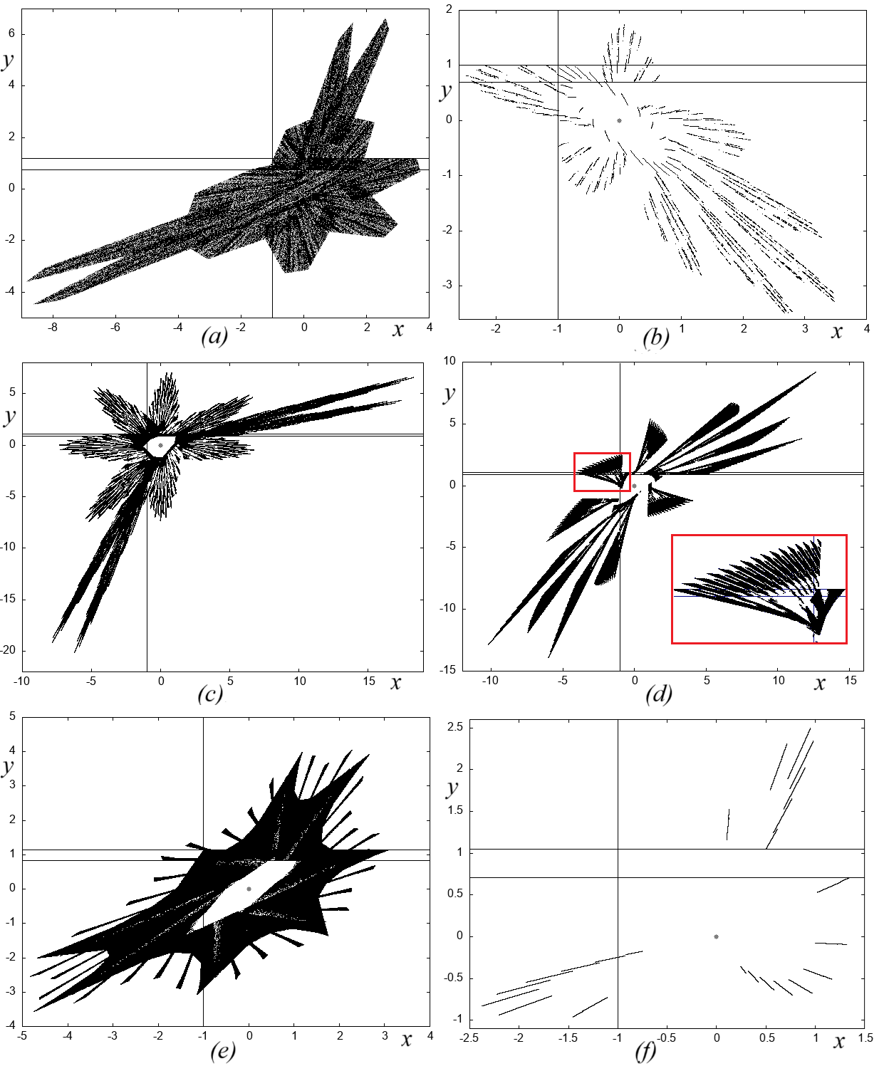
Figure 1: Attractors of map $F$ for (a) $\delta_{L}=0.75$, $\delta_{R}=1.2$, $\tau_{L}=-0.7$, $\tau_{R}=-2.5$; (b) $\delta_{L}=0.7$, $\delta_{R}=1.001$, $\tau_{L}=0.3$, $\tau_{R}=0.71$; (c) $\delta_{L}=0.9$, $\delta_{R}=1.1$, $\tau_{L}=-2.5$, $\tau_{R}=-0.7$; (d) $\delta_{L}=0.9$, $\delta_{R}=1.1$, $\tau_{L}=-2.5$, $\tau_{R}=-1.2$; (e) $\delta_{L}=0.84$, $\delta_{R}=1.15$, $\tau_{L}=-1$, $\tau_{R}=-1.9$; (f) $\delta_{L}=1.05$, $\delta_{R}=0.7$, $\tau_{L}=-0.75$, $\tau_{R}=-1.6$. Discontinuity line $x=-1$ and its images, $y=\delta_{L}$ and $y=\delta_{R},$ by maps $F_{L}$ and $F_{R},$ respectively, are also shown.

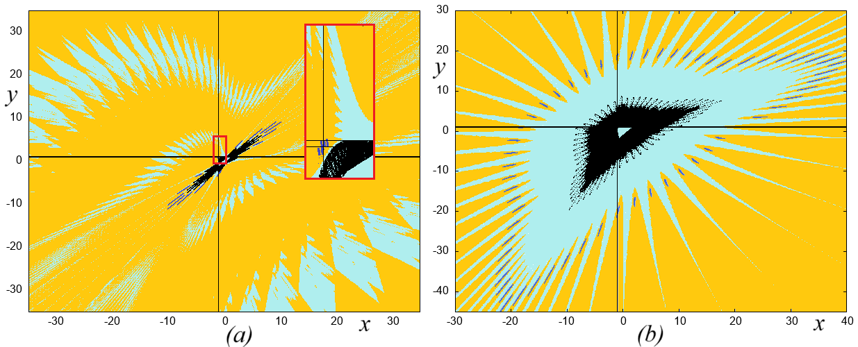
Figure 2: Two coexisting weird quasiperiodic attractors (shown in black and dark blue) of map $F$ and their basins (in light blue and yellow) for (a) $\delta_{L}=0.9$, $\delta_{R}=1.1$, $\tau_{L}=0.3$, $\tau_{R}=0.71;$ (b) $\delta_{L}=0.9$, $\delta_{R}=1.11$, $\tau_{L}=-2$, $\tau_{R}=-1.91$.

In the present paper, we consider map $F$ given in (2) as the simplest representative of a class of 2D discontinuous piecewise linear maps, defined by a finite number of linear homogeneous functions in different partitions of the phase plane, separated by smooth discontinuity curves.

A weird quasiperiodic attractor (WQA for short) $\mathcal{A}$ of map $F$ is an attractor (a closed invariant attracting set with a dense trajectory) with a rather complicated, say, weird, structure, which does not include periodic points. Thus, $\mathcal{A}$ is neither an attracting cycle nor a chaotic attractor: it is the closure of quasiperiodic trajectories. To clarify, it is worth adding a few comments:

$\bullet$ By invariance we mean that $F(\mathcal{A})=\mathcal{A}$.

$\bullet$ We use the standard (topological) definition of an attracting set, namely, a closed invariant set $A$ is attracting if there exists a neighborhood $U(A)$ of $A$ such that $T(U(A))\subset U(A)$ and ${\displaystyle\bigcap\limits_{i=0}^{\infty}}T^{i}(U(A))=A$. An attractor $\mathcal{A}$ is an attracting set with a dense trajectory.

$\bullet$ As already mentioned, for map $F$ given in (2), it is easy to show that it cannot have hyperbolic cycles (see Property 5 in the next section). This property is straightforward also for other piecewise linear homogeneous maps.

$\bullet$ It is interesting to compare a WQA with other known kinds of attractors that are also associated with quasiperiodic dynamics such as a Cantor set attractor (it can be observed, e.g., in a Lorenz map when it is a gap map, see [1]), or a critical attractor (as, e.g., in the logistic map at the Feigenbaum accumulation points, see [24]), or a strange nonchaotic attractor (SNA for short, observed in maps with quasiperiodic forcing, as described, e.g., in [15], [8] for smooth maps or in [32], [33], [7] for piecewise smooth maps). All these attractors have a fractal structure. As for the structure of a WQA, the examples shown in Figs. 1 and 2 have no fractal structure (see also other examples of WQAs in the next sections). We think that it is a characteristic property of the attractors of the considered class of maps, although it is not an easy task to prove it in a generic case.

$\bullet$ In some special cases, map $F$ can have an attractor with a rather simple structure (e.g., consisting of a finite number of segments), which can be studied by means of a 1D map (a first return map on one of the segments). We do not call such an attractor a WQA. For example, such a nongeneric case may be observed for parameter values $\delta_{L}=0$ or $\delta_{R}=0,$ when the entire partition defined by $x<0$ or $x>0,$ respectively, is mapped into the straight line $y=0.$ As shown in our companion paper [12], if a 1D first return map to a suitable segment of this straight line exists, with a finite number of discontinuity points, then this map is topologically conjugated to a piecewise linear circle map with a rational or irrational rotation number.

The paper is organized as follows. In the next section, several properties of map $F$ are stated that are useful for describing its dynamics. In Sec. 3, we present two examples of the bifurcation structure of the parameter space of map $F,$ in the $(\tau_{L},\tau_{R})$-parameter plane for $\delta_{L}=0.9,$ $\delta_{R}=0.7,$ and in the $(\delta_{R},\tau_{R})$-parameter plane for $\delta_{L}=0.9$, $\tau_{L}=-2.5$, with the regions related to the attracting fixed point in the origin, weird quasiperiodic attractors, and divergence. We obtain analytical expressions for the boundaries of the divergence regions in the simplest case related to the basic and complementary to basic symbolic sequences. In Sec. 4, we consider in detail the bifurcation structure near two specific divergence regions and discuss, by means of several examples of the phase portrait of map $F$, a mechanism of appearance of WQAs for parameters values taken near those divergence regions. Some concluding remarks are presented in Sec. 5.

2 Preliminaries

We consider a 2D discontinuous piecewise linear map $F:\mathbb{R}^{2}\rightarrow\mathbb{R}^{2},$ defined as follows:

$$F=\left\{\begin{tabular}[c]{ll}$F_{L}:\left(\begin{array}[c]{c}x\\ y\end{array}\right)\rightarrow J_{L}\left(\begin{array}[c]{c}x\\ y\end{array}\right)$&if $x<-1$\\ $F_{R}:\left(\begin{array}[c]{c}x\\ y\end{array}\right)\rightarrow J_{R}\left(\begin{array}[c]{c}x\\ y\end{array}\right)$&if $x>-1$\end{tabular}\ \ \ \ \ \ \ \right.$$ (3)

where

$$J_{L}=\left(\begin{array}[c]{cc}\tau_{L}&1\\ -\delta_{L}&0\end{array}\right),\ J_{R}=\left(\begin{array}[c]{cc}\tau_{R}&1\\ -\delta_{R}&0\end{array}\right)$$ (4)

Here, $\delta_{i}=\det J_{i},$ $\tau_{i}=trJ_{i},$ $i=L,R,$ are real parameters. Note that we could choose any vertical line defined by $x=h,$ $h\neq 0,$ as a discontinuity line, as parameter $h$ can be scaled out. Indexes $L$ and $R$ in (3) and (4) refer to the left and right partitions of the phase plane,

$$D_{L}=\left\{(x,y):x<-1\right\},\ \ D_{R}=\left\{(x,y):x>-1\right\}$$

separated by the discontinuity line

$$C_{-1}=\{(x,y):x=-1\}$$

The images of $C_{-1}$ are denoted as

$$C^{L}=F_{L}(C_{-1})=\{(x,y):y=\delta_{L}\},\ C^{R}=F_{R}(C_{-1})=\{(x,y):y=\delta_{R}\}$$

We call the discontinuity line $C_{-1},$ as well as its images and preimages, critical lines (of corresponding rank), following [21].

Let us state several properties of map $F$ that are easy to verify:

Property 1.

The fixed point $O=(0,0)\in D_{R}$ of map $F_{R}$ is the unique fixed point of map $F,$ provided no eigenvalue of $F_{R}$ equals $1,$ i.e., $1-\tau_{R}+\delta_{R}\neq 0.$

Property 2.

Invertibility of map $F$ is of

(a) $Z_{1}-Z_{0}-Z_{1}$ type for $0<\delta_{R}<\delta_{L},\$or $\delta_{L}<\delta_{R}<0;$

(b) $Z_{1}-Z_{2}-Z_{1}$ type for $\delta_{R}<\delta_{L}<0,$ or $0<\delta_{L}<\delta_{R};$

(c) $Z_{0}-Z_{1}-Z_{2}$ type for $\delta_{L}\delta_{R}<0;$

(d) $Z_{1}-Z_{\infty}-Z_{1}-Z_{0}$ type for $\delta_{L}=0,$ $\delta_{R}\neq 0;$

(e) $Z_{0}-Z_{\infty}-Z_{0}-Z_{1}$ type for $\delta_{R}=0,$ $\delta_{L}\neq 0;$

(f) $Z_{1}-Z_{2}-Z_{1}$ type for $\delta_{R}=\delta_{L}.$

This property can be verified by considering the images of halfplanes $D_{L}$ and $D_{R},$ which define regions called zones $Z_{j},$ where index $j$ indicates the number of preimages of a point in zone $Z_{j}.$ In generic cases (a), (b), or (c), zones $Z_{j}$ are separated by the critical lines $C^{L}$ and $C^{R}$. In the nongeneric cases (d) and (e), $Z_{\infty}$ is the critical line $C^{L}$ and $C^{R},$ respectively. Each point of these lines has an infinite number of preimages (a straight line), since the complete halfplane $D_{L}$ or $D_{R}$ is mapped into one straight line, $C^{L}$ or $C^{R},$ respectively. In the nongeneric case (f), $Z_{2}$ is the critical line $C^{L}=C^{R},$ whose points have two distinct preimages. For example, map $F$ has $Z_{1}-Z_{2}-Z_{1}$ type of invertibility in Figs. 1(a-e) and $Z_{1}-Z_{0}-Z_{1}$ type of invertibility in Fig. 1(f).

Property 3.

In the $(\delta_{i},\tau_{i})$-parameter plane, $i=L,R,$ the eigenvalues $\lambda_{1,2}^{i}=\frac{1}{2}(\tau_{i}\pm\sqrt{\tau_{i}^{2}-4\delta_{i}})$ of matrix $J_{i}$ satisfy $\left|\lambda_{1,2}^{i}\right|<1$ in the stability triangle $T^{i},$ defined as

$$T^{i}=\{(\delta_{i},\tau_{i}):\delta_{i}<1,\ -1-\delta_{i}<\tau_{i}<1+\delta_{i}\}$$ (5)

This triangle is bounded by the segments of the straight lines $\tau_{i}=1+\delta_{i}$ (related to $\lambda_{1}^{i}=1$), $\tau_{i}=-1-\delta_{i}$ (related to $\lambda_{2}^{i}=-1$), and $\delta_{i}=1$ (related to complex-conjugate eigenvalues $|\lambda_{1,2}^{i}|=1$).

Property 4.

For the fixed point $O,$ the boundary of the stability domain $T^{R}$ defined by $\tau_{R}=1+\delta_{R}$ corresponds to a degenerate $+1$ bifurcation, at which any point of halfline $S^{R}=\{(x,y):x>-1,\ y=-\delta_{R}x\}$ is fixed, while the boundary defined by $\tau_{R}=-1-\delta_{R}$ corresponds to a degenerate flip bifurcation, at which any point (except the fixed point $O$) of segment $S^{R^{2}}=\{(x,y):-1<x<1,\ y=\delta_{R}x\}$ is $2$-periodic. The boundary defined by $\delta_{R}=1$ corresponds to a center bifurcation of the fixed point $O,$ at which for a rational rotation number $\rho=m/n$ of matrix $J_{R},$ i.e., for $\tau_{R}=2\cos(2\pi m/n),$ there exists an invariant polygon with $n$ sides filled with nonhyperbolic cycles having rotation number $m/n,$ while if $\rho$ is irrational, there then exists an invariant region filled with quasiperiodic trajectories and bounded by an invariant ellipse tangent to the discontinuity line $C_{-1}$.

For more details on degenerate bifurcations in piecewise linear maps, we refer to [31].

Let $F_{\sigma}$ denote a composite map, $F_{\sigma}=F_{\sigma_{0}}\circ F_{\sigma_{1}}...\circ F_{\sigma_{n-1}},$ where $\sigma=\sigma_{0}\sigma_{1}...\sigma_{n-1}$ is a symbolic sequence with $\sigma_{j}\in\{L,R\},$ $n\geq 2.$ The corresponding Jacobian matrix is denoted by $J_{\sigma}$, where $J_{\sigma}={\displaystyle\prod\limits_{j=0}^{n-1}}J_{\sigma_{j}},$ and its characteristic polynomial is $P_{\sigma}(\lambda)=\lambda^{2}-trJ_{\sigma}\lambda+\det J_{\sigma}=0.$ It is easy to see that the fixed point equation $F_{\sigma}(x,y)=(x,y)$ has a unique solution $(x,y)=(0,0),$ provided that $P_{\sigma}(1)\neq 0$ (i.e., matrix $J_{\sigma}$ has no eigenvalue $1$), so that the unique hyperbolic fixed point of $F_{\sigma}$ for any $\sigma$ is the fixed point $O.$ Thus, the following property holds:

Property 5.

Map $F$ cannot have cycles of period $n$ for any $n\geq 2,$ except for nonhyperbolic $n$-cycles with an eigenvalue equal to $1$.

Nonhyperbolic $n$-cycles with one eigenvalue equal to $1$ (not related to the fixed point $O$), associated with condition $P_{\sigma}(1)=0,$ fill densely specific segments, bounded or one-side unbounded. More precisely, let the eigenvalues of matrix $J_{\sigma}$ be real and distinct (i.e., $(trJ_{\sigma})^{2}-4\det J_{\sigma}>0$), and let the corresponding eigenvectors be denoted by $V^{\sigma}$ and $W^{\sigma}.$ Consider eigenvector $V^{\sigma}$ and its $n-1$ images by map $F$ (all these sets obviously belong to straight lines through the origin). Suppose the following admissibility property is satisfied: there exists a subset of $V^{\sigma}$ located in partition $D_{\sigma_{0}}$ such that its $n-1$ images by $F$ are all located in the proper partitions, according to the symbolic sequence $\sigma$. Let $\{V_{j}^{\sigma}\}_{j=0}^{n-1}$ be a maximal admissible set. This means that there is a subset of $V^{\sigma}$ denoted by $V_{0}^{\sigma}$ belonging to $D_{\sigma_{0}}$ such that $F^{j}(V_{0}^{\sigma})=:$ $V_{j}^{\sigma}\subset D_{\sigma_{j}}$ for all $j=\overline{1,n-1},$ moreover, one boundary point of (at least) one of the sets $V_{j}^{\sigma}$ belongs to the discontinuity line $C_{-1}.$ The latter property implies that all the other boundary points of the sets $V_{j}^{\sigma}$ are images of this point (or these points). Now, let $P_{\sigma}(1)=0,$ i.e., one eigenvalue of matrix $J_{\sigma}$ equals $1,$ and let $V^{\sigma}$ be the corresponding eigenvector (for matrix $J_{\sigma}$ it is a straight line through the origin filled with the fixed points). Then we can state the following

Property 6.

Map $F$ has a maximal admissible set of $n$ cyclic segments (bounded or one-side unbounded), say, $S^{\sigma}=\{S_{j}^{\sigma}\}_{j=0}^{n-1},$ $n\geq 2,$ filled with nonhyperbolic $n$-cycles (with eigenvalue $+1$) having symbolic sequence $\sigma,$ provided that $P_{\sigma}(1)=0,$ $\det J_{\sigma}\neq 1,$ and $S_{j}^{\sigma}=V_{j}^{\sigma}\subset D_{\sigma_{j}}$ for all $j=\overline{0,n-1}.$

Obviously, set $S^{\sigma}$ is not robust, i.e., it does not persist under parameter perturbations. Put differently, the Lebesgue measure of the parameter set satisfying $P_{\sigma}(1)=0$ is zero. Below, for short, we denote a nonhyperbolic cycle having symbolic sequence $\sigma$ as $\sigma$-cycle. Examples of one-side unbounded segments $\{S_{j}^{\sigma}\}_{j=0}^{n-1}$ for various $\sigma$ can be seen in Fig. 6(b),(e), Fig. 7(a), and Fig. 9(a), while bounded segments are shown in Fig. 10(a) and Fig. 13(a).

Since map $F$ cannot have hyperbolic cycles, it cannot have chaotic attractors either. Thus, we can state that in a generic case, a bounded attractor of map $F$ is either the fixed point $O$ or a WQA. Note that set $S^{\sigma},$ consisting of $n$ cyclic segments filled with nonhyperbolic $\sigma$-cycles (see Property 6), may be an attracting set, but it is not an attractor since it does not include a dense trajectory. As mentioned in the Introduction, an example of a nongeneric case may also be related to parameter values $\delta_{R}=0$ or $\delta_{L}=0,$ when an attractor of map $F$ may be studied by means of a 1D first return map (see [12] for details).

With regard to the possible coexistence of attractors of map $F$, examples of two coexisting WQAs are presented in Figs. 2 and 12(b), while examples of an attracting fixed point $O$ coexisting with a WQA are shown in Figs. 6(c),(f), 9(b), and 10(b).

As we will demonstrate in the next section, some boundaries of a region in the parameter space, associated with WQAs of map $F$, are related to the existence of specific sets $S^{\sigma}.$ As an example, we will consider basic symbolic sequences, $\sigma=LR^{n-1}$ and $\sigma=RL^{n-1},$ $n\geq 3,$ assuming the simplest case of rotation number $\rho=1/n,$ as well as symbolic sequences that are complementary to these sequences, namely, $\sigma=L^{2}R^{n-2}$ and $\sigma=R^{2}L^{n-2},$ respectively. Here, considering a (nonhyperbolic) cycle with a symbolic sequence $\sigma,$ by its rotation number $\rho=m/n,$ we mean that along the cycle the trajectory makes $m$ turns around the origin in $n$ iterations.

3 Bifurcation structure of map $F$:
weird quasiperiodic attractors and divergence

In Fig. 3(a), we present the bifurcation structure of map $F$ in the $(\tau_{L},\tau_{R})$-parameter plane for $\delta_{L}=0.9,$ $\delta_{R}=0.7$. Similarly, Fig. 3(b) shows the bifurcation structure of map $F$ in the $(\delta_{R},\tau_{R})$-parameter plane for $\delta_{L}=0.9,$ $\tau_{L}=-2.5.$ In these figures, blue and yellow regions indicate convergence of an initial point to the fixed point $O$ and to a WQA, respectively, while gray regions indicate divergence. For parameter values as in Fig. 3(a), map $F$ has $Z_{1}-Z_{0}-Z_{1}$ invertibility type since $0<\delta_{R}<\delta_{L}$ (see Property 2(a)). In Fig. 3(b), map $F$ has $Z_{0}-Z_{1}-Z_{2}$ invertibility type for $\delta_{R}<0$ (Property 2(c)), $Z_{1}-Z_{0}-Z_{1}$ invertibility type for $0<\delta_{R}<0.9$ (Property 2(a)), $Z_{1}-Z_{2}-Z_{1}$ invertibility type for $\delta_{R}>0.9$ (Property 2(b)), and in special cases, it is of $Z_{0}-Z_{\infty}-Z_{0}-Z_{1}$ invertibility type for $\delta_{R}=0$ (Property 2(e)), and $Z_{1}-Z_{2}-Z_{1}$ invertibility type for $\delta_{R}=\delta_{L}=0.9$ (Property 2(f)).

For $\delta_{R}=0.7,$ as in Fig. 3(a), the fixed point $O$ is attracting in the horizontal strip $-1.7<\tau_{R}<1.7,$ while in Fig. 3(b), it is attracting for parameter values belonging to the indicated stability triangle $T^{R}$ (see (5)). In both figures, the fixed point $O$ can be globally attracting or coexisting either with a WQA, with divergent trajectories, or with segments filled with nonhyperbolic cycles.

In fact, the boundaries of the divergence regions that satisfy conditions $P_{\sigma}(1)=0$ for specific $\sigma$ are related to the existence of $n$ cyclic halflines, $S^{\sigma}=\{S_{j}^{\sigma}\}_{j=0}^{n-1},$ $n\geq 2,$ filled with points of nonhyperbolic $\sigma$-cycles (see Property 6). Below we obtain the boundaries of the divergence regions, denoted by $D_{1/n}^{R},$ associated with the basic and complementary to basic symbolic sequences $\sigma=LR^{n-1}$ and $\sigma=L^{2}R^{n-2}$, as well as the boundaries of the divergence regions, denoted by $D_{1/n}^{L},$ associated with symbolic sequences $\sigma=RL^{n-1}$ and $\sigma=R^{2}L^{n-2}$. The lower index $1/n$ means that in the considered case, the rotation number is $\rho=1/n.$ The boundaries of regions $D_{1/n}^{R}$ and $D_{1/n}^{L}$ in Fig. 3(a) and the boundaries of regions $D_{1/n}^{R}$ in Fig. 3(b) are shown for $n=2,...,9.$ In Fig. 4, the 1D bifurcation diagrams, showing $x$ versus $\tau_{L}$ in (a) and $y$ versus $\tau_{L}$ in (b), illustrate the dynamics of map $F$ for fixed $\tau_{R}=-2$ and increasing $\tau_{L}.$ It can be seen that the divergence regions $D_{1/n}^{L}$ (with no bounded dynamics) are crossed, and the regions between them correspond to WQAs. Note that for $\tau_{R}=-2,$ the fixed point $O$ is a saddle.

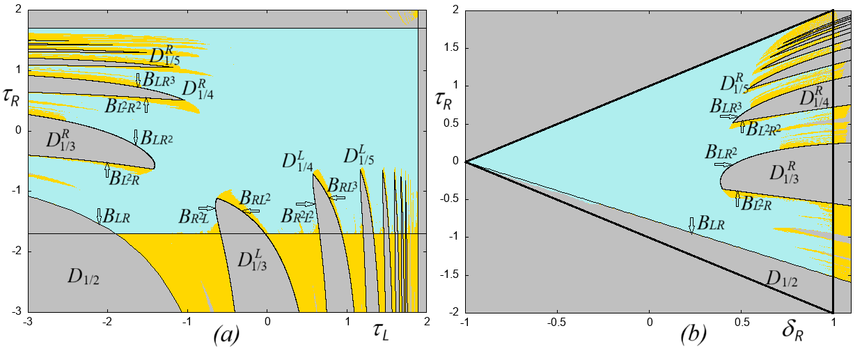
Figure 3: Bifurcation structure of map $F$ (a) in the $(\tau_{L},\tau_{R})$-parameter plane for $\delta_{L}=0.9,$ $\delta_{R}=0.7$ , and (b) in the $(\delta_{R},\tau_{R})$-parameter plane for $\delta_{L}=0.9,$ $\tau_{L}=-2.5$. The boundaries $B_{LR^{n-1}}$ and $B_{L^{2}R^{n-2}}$ of the divergence region $D_{1/n}^{R},$ defined in (12) and (13), respectively, and the boundaries $B_{RL^{n-1}}$ and $B_{R^{2}L^{n-2}}$ of the divergence region $D_{1/n}^{L}$ defined in (16) and (18), respectively, are shown for $n=2,...,9.$ Blue and yellow parameter regions indicate convergence to the fixed point $O$ and to a WQA, respectively. Gray regions indicate divergence.

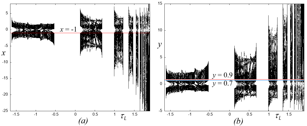
Figure 4: A 1D bifurcation diagram of map $F$ showing $x$ versus $\tau_{L}$ in (a), and $y$ versus $\tau_{L}$ in (b) for $\delta_{L}=0.9,$ $\delta_{R}=0.7,$ and $\tau_{R}=-2.$

The divergence regions mentioned above are closely related to the so-called dangerous bifurcations occurring in the 2D border collision normal form $G_{\mu}$. These bifurcations were studied quite intensively due to their importance in the applied context (see, e.g., [16], [9], [5], [6], [10], [2]). Recall that in the 2D border collision normal form $G_{\mu}$ defined in (1), a dangerous bifurcation occurs at $\mu=0$ if for $\mu<0$ and for $\mu>0$ an attractor or several attractors of map $G_{\mu}$ coexist with divergent trajectories (i.e., with an attractor at infinity). In this case, as $\mu$ tends to $0,$ any attractor and its basin decrease in size linearly with respect to $\mu$, and at $\mu=0,$ they shrink to point $(x,y)=(0,0).$ At $\mu=0,$ the generic trajectory thus diverges. As a result, there exists one or several attractors before and after the bifurcation, i.e., for $\mu<0$ and $\mu>0,$ but near $\mu=0,$ the basins of bounded trajectories become quite small, so that even small perturbations may lead to divergence, motivating the name dangerous bifurcation.

A necessary condition for a dangerous bifurcation to occur is the coexistence of a bounded attractor with an attractor at infinity, which can be studied using compactification of the phase plane (see, e.g., [27]). Recall that in the parameter space of map $G_{\mu},$ the boundaries of the divergence regions related to dangerous bifurcations satisfy conditions $P_{\sigma}(1)=0$ for specific symbolic sequences $\sigma,$ as well as the corresponding admissibility conditions. Crossing the boundary of a divergence region defined by $P_{\sigma}(1)=0$ for some fixed $\mu\neq 0,$ an $n$-cycle of map $G_{\mu}$ with symbolic sequence $\sigma$ undergoes a degenerate transcritical bifurcation: its points tend to infinity while an eigenvalue tends to $1.$ For $\mu=0,$ a kind of degenerate $+1$ bifurcation occurs: there are $n$ stable and $n$ unstable invariant halflines issuing from the fixed point in the origin, and these halflines are filled with points of nonhyperbolic $\sigma$-cycles. We refer to [9], [10], and [2] for more details related to the dangerous bifurcation in map $G_{\mu},$ occurring at $\mu=0.$ In any case, condition $P_{\sigma}(1)=0$ depends only on the parameters of matrices $J_{L}$ and $J_{R}$, i.e., from $\tau_{i}$ and $\delta_{i},$ $i=L,R.$ These matrices are defined in the same way for both maps $G_{\mu}$ and $F$, confirming an intuitive idea about the similarity of the dynamics of maps $G_{\mu}$ and $F$ at infinity. However, map $F$ is discontinuous, and its border line is not $x=0$ but $x=-1,$ which leads to some specific new properties mentioned below.

Let us obtain the boundaries of the divergence regions (satisfying conditions $P_{\sigma}(1)=0$) in the parameter space of map $F$ by considering the simplest case, namely, regions $D_{1/n}^{R}$ associated with symbolic sequences $\sigma=LR^{n-1}$ and $\sigma=L^{2}R^{n-2},$ $n\geq 3,$ and regions $D_{1/n}^{L}$ associated with $\sigma=RL^{n-1}$ and $\sigma=R^{2}L^{n-2}.$

3.1 $\sigma=LR^{n-1},$ $n\geq 3$

Consider first a composite map $F_{\sigma}$ with $\sigma=LR^{n-1},$ $n\geq 3.$ Matrix $J_{LR^{n-1}}=J_{R}^{n-1}J_{L}$ can be defined as follows:

$$J_{LR^{n-1}}=\left(\begin{array}[c]{cc}a_{n-1}&a_{n-2}\\ -\delta_{R}a_{n-2}&-\delta_{R}a_{n-3}\end{array}\right)\left(\begin{array}[c]{cc}\tau_{L}&1\\ -\delta_{L}&0\end{array}\right)=$$

$$\left(\begin{array}[c]{cc}\tau_{L}a_{n-1}-\delta_{L}a_{n-2}&a_{n-1}\\ -\tau_{L}\delta_{R}a_{n-2}+\delta_{L}\delta_{R}a_{n-3}&-\delta_{R}a_{n-2}\end{array}\right)$$

where $a_{k}$ is the solution of the second-order homogeneous linear difference equation

$$a_{k}=\tau_{R}a_{k-1}-\delta_{R}a_{k-2},\ \ a_{0}=1,\ \ a_{1}=\tau_{R},\ k=2,3,...$$

The eigenvalues

$$\lambda_{1,2}^{LR^{n-1}}=0.5(\tau_{L}a_{n-1}-(\delta_{L}+\delta_{R})a_{n-2}\pm\sqrt{(\tau_{L}a_{n-1}-(\delta_{L}+\delta_{R})a_{n-2})^{2}-4\delta_{L}\delta_{R}^{n-1}})$$

of matrix $J_{LR^{n-1}}$ are real if $(\tau_{L}a_{n-1}-(\delta_{L}+\delta_{R})a_{n-2})^{2}-4\delta_{L}\delta_{R}^{n-1}>0,$ and the corresponding eigenvectors have slopes

$$K_{i}^{LR^{n-1}}=\frac{\delta_{R}(\delta_{L}a_{n-3}-\tau_{L}a_{n-2})}{\delta_{R}a_{n-2}+\lambda_{i}},\ i=1,2$$ (6)

Transition from real to complex-conjugate eigenvalues occurs crossing a parameter set denoted $E_{LR^{n-1}}$ and defined as follows:

$$E_{LR^{n-1}}:\ \ (\tau_{L}a_{n-1}-(\delta_{L}+\delta_{R})a_{n-2})^{2}-4\delta_{L}\delta_{R}^{n-1}=0$$ (7)

The characteristic polynomial of $J_{LR^{n-1}}$ can be written as follows:

$$P_{LR^{n-1}}(\lambda)=\lambda^{2}+\left(-\tau_{L}a_{n-1}+(\delta_{L}+\delta_{R})a_{n-2}\right)\lambda+\delta_{L}\delta_{R}^{n-1}$$ (8)

Considering the linear map $F_{LR^{n-1}},$ i.e., map $F_{LR^{n-1}}:(x,y)\rightarrow J_{LR^{n-1}}(x,y),$ without its relation to the piecewise linear map $F$, condition $P_{LR^{n-1}}(1)=0$ (for $\delta_{L}\delta_{R}^{n-1}\neq 1$) means that map $F_{LR^{n-1}}$ has an eigenvalue equal to $1$ and the straight line through the origin, say $y=K^{LR^{n-1}}x,$ associated with the corresponding eigenvector, is filled with fixed points, where

$$K^{LR^{n-1}}=\frac{\delta_{R}(\delta_{L}a_{n-3}-\tau_{L}a_{n-2})}{\delta_{R}a_{n-2}+1}$$ (9)

However, considering the piecewise linear map $F$, condition

$$P_{LR^{n-1}}(1)=1-\tau_{L}a_{n-1}+(\delta_{L}+\delta_{R})a_{n-2}+\delta_{L}\delta_{R}^{n-1}=0$$ (10)

is necessary but not sufficient for the existence of set $S^{LR^{n-1}}$ consisting of $n$ segments filled with points of nonhyperbolic $LR^{n-1}$-cycles. According to Property 6, the admissibility conditions must be satisfied, that is, these segments must be located in the proper partitions. Here we are interested in the boundaries of the divergence regions, so these segments are halflines and their ”end points at infinity” are, for the compactified map, periodic as well, with symbolic sequence $LR^{n-1}.$ In the considered case, denoting the starting halfline belonging to $D_{L}$ as $S_{0}^{LR^{n-1}},$ so that

$$S_{0}^{LR^{n-1}}=\{(x,y):y=K^{LR^{n-1}}x,\ x<-1\}$$

(assuming $K^{LR^{n-1}}\neq\infty,$ that is, $\delta_{R}a_{n-2}+1\neq 0$, see (9), that holds for $\delta_{R}\neq 1$), its images $S_{j}^{LR^{n-1}}=F(S_{j-1}^{LR^{n-1}})$ for $j=\overline{1,n-1}$ must be completely located in partition $D_{R}$. For short, we denote these admissibility conditions as $(A^{LR^{n-1}})$, that is,

$$(A^{LR^{n-1}}):\ \ S_{0}^{LR^{n-1}}\subset D_{L},\ S_{j}^{LR^{n-1}}\subset D_{R},\ \text{ }j=\overline{1,n-1}$$ (11)

(an example of admissible set $S^{LR^{4}}$ consisting of five halflines filled with nonhyperbolic $LR^{4}$-cycles is shown in Fig. 6(a)).

In contrast to the map $G_{0}$, map $F$ can also have a set $S^{LR^{n-1}}$ satisfying condition $P_{LR^{n-1}}(1)=0$ and admissibility conditions $(A^{LR^{n-1}})$, but consisting of bounded segments (see Fig. 7(a) for an example), and in such a case the corresponding parameter set is not associated with the boundary of a divergence region (see the point marked $g$ in Fig. 5(a) corresponding to Fig. 7(a)). In fact, comparing with map $G_{0}$, in map $F$ the border line is shifted to the left, from $x=0$ to $x=-1,$ so that partition $D_{R}$ is enlarged, providing additional space for the segments of set $S^{LR^{n-1}}$ to be still admissible, which in the case of map $G_{0}$ would be not admissible (or, in other words, virtual).

To summarize, we can state that among the parameter values satisfying $P_{LR^{n-1}}(1)=0$ given in (10), there may be a subset denoted $B_{LR^{n-1}}$ that satisfies the admissibility conditions $(A^{LR^{n-1}})$ given in (11):

$$B_{LR^{n-1}}:\ \ 1-\tau_{L}a_{n-1}+(\delta_{L}+\delta_{R})a_{n-2}+\delta_{L}\delta_{R}^{n-1}=0\text{ and }(A^{LR^{n-1}})\text{ holds}$$ (12)

where segments $S_{j}^{LR^{n-1}},\$ $j=\overline{1,n-1},$ in $(A^{LR^{n-1}})$ can be either one-side unbounded (then $B_{LR^{n-1}}$ belongs to a boundary of the divergence region $D_{1/n}^{R}$), or bounded.

3.2 $\sigma=L^{2}R^{n-2},$ $n\geq 3$

Following analogous steps for the complementary symbolic sequence $\sigma=L^{2}R^{n-2},$ we obtain a set of parameter values, denoted by $B_{L^{2}R^{n-2}},$ satisfying $P_{L^{2}R^{n-2}}(1)=0,$ and the corresponding admissibility conditions:

$$B_{L^{2}R^{n-2}}:\ \ 1+(\tau_{L}(\delta_{L}+\delta_{R})-\delta_{L}\tau_{R})a_{n-3}-(\tau_{L}^{2}-2\delta_{L})a_{n-2}+\delta_{L}^{2}\delta_{R}^{n-2}=0$$

$$\text{ and }(A^{L^{2}R^{n-2}})\text{ holds}$$ (13)

where

$$(A^{L^{2}R^{n-2}}):\ \ S_{0}^{L^{2}R^{n-2}}\subset D_{L},\ S_{1}^{L^{2}R^{n-2}}\subset D_{L},\ S_{j}^{L^{2}R^{n-2}}\subset D_{R},\text{ }j=\overline{2,n-1}$$

and

$$S_{0}^{L^{2}R^{n-2}}=\{(x,y):y=K^{L^{2}R^{n-2}}x,\ x<-1\}$$

with

$$K^{L^{2}R^{n-2}}=\frac{\delta_{R}(\delta_{L}a_{n-3}+\tau_{L}\left(\delta_{L}a_{n-4}-\tau_{L}a_{n-3}\right))}{\delta_{R}(\tau_{L}a_{n-3}-\delta_{L}a_{n-4})+1}$$

(see an example of set $S^{L^{2}R^{3}}$ consisting of five halflines filled with nonhyperbolic $L^{2}R^{3}$-cycles in Fig. 6(d)).

In this way, two boundaries, $B_{LR^{n-1}}$ and $B_{L^{2}R^{n-2}},$ of the divergence region $D_{1/n}^{R},$ $n\geq 3,$ are obtained (see Fig. 3).

Note that for a parameter point belonging to region $D_{1/n}^{R},$ map $F$ has an attracting $n$-cycle at infinity with symbolic sequence either $LR^{n-1}$ or $L^{2}R^{n-2},$ associated with the unstable eigenvector of matrix $J_{LR^{n-1}}$ or $J_{L^{2}R^{n-2}},$ respectively, and its $n-1$ images by map $F$ (see, e.g., vectors $V_{j}^{LR^{4}}$ and $V_{j}^{L^{2}R^{3}},$ $j=\overline{0,4}$, in Fig. 6(a) and (d), respectively). A boundary, say $H_{LR^{n-1}},$ separating the corresponding subregions of region $D_{1/n}^{R}$ can be defined by the condition that the eigenvector of matrix $J_{LR^{n-1}}$ has slope $0$ (and, thus, the slope of its preimage by $F_{R}$ is equal to infinity). Then, for a parameter point belonging to region $D_{1/n}^{R},$ we have the following:

$\bullet$ on one side of boundary $H_{LR^{n-1}},$ it holds that the unstable eigenvectors $V_{j}^{LR^{n-1}}$ are admissible, while eigenvectors $V_{j}^{L^{2}R^{n-2}}$ are not admissible (so that an attracting $LR^{n-1}$-cycle at infinity exists, while the $L^{2}R^{n-2}$-cycle is virtual);

$\bullet$ on the other side of boundary $H_{LR^{n-1}}$, the unstable eigenvectors $V_{j}^{L^{2}R^{n-2}}$ are admissible, while eigenvectors $V_{j}^{LR^{n-1}}$ are not admissible (so that an attracting $L^{2}R^{n-2}$-cycle at infinity exists, while the $LR^{n-1}$-cycle is virtual).

So, assuming that in (6) $\delta_{R}\neq 0,$ from $K_{i}^{LR^{n-1}}=0$ boundary $H_{LR^{n-1}}$ can be defined as follows:

$$H_{LR^{n-1}}:\ \ \delta_{L}a_{n-3}-\tau_{L}a_{n-2}=0,\ \ H_{LR^{n-1}}\subset D_{1/n}^{R}$$ (14)

Transition from real to complex-conjugate eigenvalues of matrix $J_{L^{2}R^{n-2}}$ (when map $F$ has no cycles at infinity) occurs crossing a parameter set

$$E_{L^{2}R^{n-2}}:\ ((\delta_{L}\tau_{R}-\tau_{L}(\delta_{L}+\delta_{R}))a_{n-3}+(\tau_{L}^{2}-2\delta_{L})a_{n-2})-4\delta_{L}^{2}\delta_{R}^{n-2}=0$$ (15)

As an example, region $D_{1/5}^{R}$ is shown magnified in Fig. 5(a), where besides its boundaries $B_{LR^{4}}$ and $B_{L^{2}R^{3}},$ also curves $H_{LR^{4}},$ $E_{LR^{4}},$ and $E_{L^{2}R^{3}}$ are shown, given in (14), (7), and (15), respectively.

3.3 $\sigma=RL^{n-1}$ and $\sigma=R^{2}L^{n-2},$ $n\geq 3$

Analogous boundaries associated with the divergence regions $D_{1/n}^{L}$ and symbolic sequences $\sigma=RL^{n-1}$ and $\sigma=R^{2}L^{n-2}$ can be obtained by changing $L\leftrightarrow R$ in all the above notations. In particular, the boundary $B_{RL^{n-1}}$ of divergence regions $D_{1/n}^{L}$ can be defined as

$$B_{RL^{n-1}}:\ \ 1-\tau_{R}b_{n-1}+(\delta_{R}+\delta_{L})b_{n-2}+\delta_{R}\delta_{L}^{n-1}=0\text{ and }(A^{RL^{n-1}})\text{ holds}$$ (16)

where the admissibility conditions $(A^{RL^{n-1}})$ are as follows:

$$(A^{RL^{n-1}}):\ \ S_{0}^{RL^{n-1}}\subset D_{R},\ S_{j}^{RL^{n-1}}\subset D_{L},\ \text{ }j=\overline{1,n-1}$$

and $b_{k}$ is a solution of the second-order homogeneous linear difference equation

$$b_{k}=\tau_{L}b_{k-1}-\delta_{L}b_{k-2},\ \ b_{0}=1,\ \ b_{1}=\tau_{L},\ \ k=2,3,...$$

Transition from real to complex-conjugate eigenvalues of matrix $J_{RL^{n}}$ is associated with crossing a parameter set $E_{RL^{n-1}}$ satisfying

$$E_{RL^{n-1}}:\ \ (\tau_{R}b_{n-1}-(\delta_{L}+\delta_{R})b_{n-2})^{2}-4\delta_{R}\delta_{L}^{n-1}=0$$ (17)

The boundary $B_{R^{2}L^{n-2}}$ of divergence regions $D_{1/n}^{L}$ can be defined as

$$B_{R^{2}L^{n-2}}:\ \ 1+(\tau_{R}(\delta_{L}+\delta_{R})-\delta_{R}\tau_{L})b_{n-3}-(\tau_{R}^{2}-2\delta_{R})b_{n-2}+\delta_{R}^{2}\delta_{L}^{n-2}=0$$

$$\text{ \ and }(A^{R^{2}L^{n-2}})\text{ holds}$$ (18)

where

$$(A^{R^{2}L^{n-2}}):\ \ S_{0}^{R^{2}L^{n-2}}\subset D_{R},\ S_{1}^{R^{2}L^{n-2}}\subset D_{R},\ S_{j}^{R^{2}L^{n-2}}\subset D_{L},\text{ }j=\overline{2,n-1}$$

Transition from real to complex-conjugate eigenvalues of matrix $J_{R^{2}L^{n-2}}$ are associated with a parameter set

$$E_{R^{2}L^{n-2}}:\ ((\delta_{R}\tau_{L}-\tau_{R}(\delta_{R}+\delta_{L}))b_{n-3}+(\tau_{R}^{2}-2\delta_{R})b_{n-2})-4\delta_{R}^{2}\delta_{L}^{n-2}=0$$ (19)

and boundary $H_{RL^{n-1}}$ can be defined as follows:

$$H_{RL^{n-1}}:\ \ \delta_{R}b_{n-3}-\tau_{R}b_{n-2}=0,\ \ H_{RL^{n-1}}\subset D_{1/n}^{L}$$ (20)

Figure 8(a) presents an example of the divergence region $D_{1/5}^{L}$ together with its boundaries $B_{RL^{4}}$ and $B_{R^{2}L^{3}},$ as well as the curves $H_{RL^{4}},\ E_{RL^{4}},$ and $E_{R^{2}L^{3}}$, given in (16), (18), (17), (19), and (20), respectively.

Note that substituting $n=2$ either to (12) or (16) the boundary $B_{LR}$ of the divergence region $D_{1/2}$ can be obtained:

$$B_{LR}:\ \ 1-\tau_{R}\tau_{L}+\delta_{R}+\delta_{L}+\delta_{R}\delta_{L}=0,\text{ \ }S_{0}^{LR}\in D_{L},\ S_{1}^{LR}\in D_{R}$$

(see Fig. 3), where $S_{0}^{LR}=\{(x,y):y=-\frac{\tau_{L}\delta_{R}}{1+\delta_{R}}x,\ x<-1\}$ and $S_{1}^{LR}=\{(x,y):y=-\frac{\tau_{R}\delta_{L}}{1+\delta_{L}}x,\ x>-\frac{\tau_{L}}{1+\delta_{R}}\}.$

In the next section, the dynamics near regions $D_{1/5}^{R}$ and $D_{1/5}^{L},$ associated with WQAs, is described in more detail.

4 Appearance of weird quasiperiodic attractors near divergence regions

4.1 Dynamics of map $F$ near the divergence region $D_{1/5}^{R}$

Let us describe the dynamics of map $F$ near the divergence region $D_{1/5}^{R}$ by considering this region in the $(\tau_{L},\tau_{R})$-parameter plane for $\delta_{L}=0.9,$ $\delta_{R}=0.7$ to see how its boundaries, $B_{LR^{4}}$ given in (12) and $B_{L^{2}R^{3}}$ given in (13), are related to the appearance of WQAs. In Fig. 5(a), the bifurcation structure near the divergence region $D_{1/5}^{R}$ is shown magnified. Besides curves $B_{LR^{4}}$ and $B_{L^{2}R^{3}},$ also curves $H_{LR^{4}}$, $E_{LR^{4}}$ and $E_{L^{2}R^{2}}$ given in (14), (7), and (15), respectively, are shown. Note that in the considered case, the complete region $D_{1/5}^{R}$ is inside the stability domain of the fixed point $O,$ so that in all the examples below the fixed point $O$ is attracting. Note also that map $F$ has $Z_{1}-Z_{0}-Z_{1}$ type of invertibility (see Property 2(a)), and it is not difficult to show that any invariant set of map $F$ cannot have points in zone $Z_{0}$ (i.e., in the strip between the critical lines $C^{R}$ and $C^{L}$), or in any image of $Z_{0}$.

Figure 5(b) illustrates the dynamics by means of a 1D bifurcation diagram showing $x$ versus $\tau_{R}$ for fixed $\tau_{L}=-2.$ At first glance, this bifurcation diagram can be misleading because the attractors here seem chaotic. However, as already mentioned, map $F$ cannot have chaotic attractors, and the limit sets we observe here are WQAs born when either boundary $B_{LR^{4}}$ (for increasing $\tau_{R}$ from a point inside the region) or boundary $B_{L^{2}R^{3}}$ (for decreasing $\tau_{R}$) is crossed. The mechanism of appearance of such attractors is illustrated in Fig. 6(a),(b),…,(f), presenting phase portraits of map $F$ at the parameter values marked in Fig. 5(a) by $a,$ $b$, …, $f,$ respectively. One more example is shown in Fig. 7, associated with the parameter point marked in Fig. 5(a) by $g$. In all these figures, the basin of the fixed point $O$ is shown in light blue, the basin of a WQA in dark yellow, the basin of a set of segments filled with nonhyperbolic cycles in light yellow, and the basin of diverging trajectories in gray.

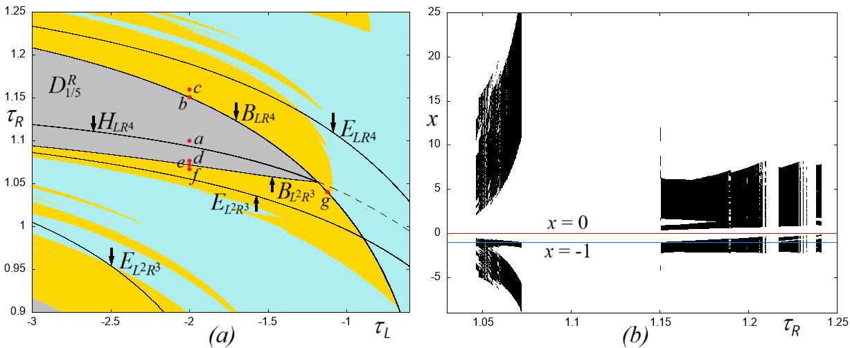
Figure 5: (a) The existence regions (in yellow) of the WQAs near the divergence region $D_{1/5}^{R}$ (in gray) bounded by curves $B_{LR^{4}}$ and $B_{L^{2}R^{3}}$ in the $(\tau_{L},\tau_{R})$-parameter plane for $\delta_{L}=0.9,$ $\delta_{R}=0.7;$ (b) 1D bifurcation diagram $x$ versus $\tau_{R}$ for $\tau_{L}=-2$. The phase portrait of map $F$ at parameter points marked in (a) by $a,$ $b,$ …, $f$ is shown in Fig. 6(a),(b),…,(f), respectively, and by $g$ in Fig. 7(a).

$\bullet$ Let us begin with the parameter point $a.$ The corresponding phase portrait of map $F$ is shown in Fig. 6(a). The parameter point $a$ is located below curve $B_{LR^{4}}$ but above curve $H_{LR^{4}}$. In this subregion of $D_{1/5}^{R},$ the attracting fixed point $O$ coexists with divergent trajectories. More precisely, it holds that $P_{LR^{4}}(1)<0,$ i.e., one eigenvalue of matrix $J_{LR^{4}}$ is larger than $1$ (the second eigenvalue is obviously positive and less than $1$); moreover, the corresponding invariant unstable halflines of map $F$ (shown in dark blue in Fig. 6(a)) are located in the proper partitions: $V_{0}^{LR^{4}}\subset D_{L}$, $V_{j}^{LR^{4}}\subset D_{R},$ $j=\overline{1,4}.$

The left column in Fig. 6 illustrates how the phase portrait of map $F$ changes for increasing values of $\tau_{R},$ when the parameter point approaches boundary $B_{LR^{4}}$ (at which $P_{LR^{4}}(1)=0$) and crosses it (so that $P_{LR^{4}}(1)>0$ holds).

$\bullet$ Parameter point $b.$ Fig. 6(b) shows the corresponding phase portrait of map $F$, where besides the attracting fixed point $O$ there exists a set $S^{LR^{4}}$ consisting of five cyclic halflines, $S_{0}^{LR^{4}}\subset D_{L}$ and $S_{j}^{LR^{4}}\subset D_{R},$ $j=\overline{1,4},$ filled with nonhyperbolic $LR^{4}$-cycles, $S_{j}^{LR^{4}}=V_{j}^{LR^{4}}$ (see Property 6).

$\bullet$ Parameter point $c.$ Fig. 6(c) presents the phase portrait after crossing boundary $B_{LR^{4}}$, where the attracting fixed point $O$ coexists with a WQA denoted $\mathcal{A}$, which appears after crossing $B_{LR^{4}}$. The mechanism of creation of attractor $\mathcal{A}$ can be outlined as follows. First, note that the parameter point $c$ is above curve $B_{LR^{4}}$ but below curve $E_{LR^{4}}$. Hence, the eigenvalues of matrix $J_{LR^{4}}$ are both real, positive, and less than $1.$ Eigenvectors $V_{j}^{LR^{4}},$ $j=\overline{0,4},$ which were forward invariant and repelling before the crossing $B_{LR^{4}}$, become attracting after the crossing. Consider halfline $V_{0}^{LR^{4}}\subset D_{L}$ (shown in blue in the inset in Fig. 6(c)). Its image $V_{5}^{LR^{4}}=F_{LR^{4}}(V_{0}^{LR^{4}})$ necessarily intersects the discontinuity line. Then, under further iterations, a part of halfline $V_{5}^{LR^{4}}$ located in $D_{L},$ say, halfline $V_{5}^{LR^{4}}|_{D_{L}},$ is mapped as before by $F_{L}$ into a halfline issuing from $C^{L}$ in $D_{R},$ while a segment of halfline $V_{5}^{LR^{4}}$ located in $D_{R},$ say segment $V_{5}^{LR^{4}}|_{D_{R}},$ is mapped by $F_{R}$ into a new segment issuing from $C^{R},$ which in this example belongs to $D_{L}.$ Next iterations of segment $V_{5}^{LR^{4}}|_{D_{R}}$ lead to further new segments approaching $V_{j}^{LR^{4}}$, $j=\overline{0,4}$, as the number of iterations tends to infinity (but they are never mapped exactly into these halflines). The resulting attractor $\mathcal{A}$ is a WQA, and it can be seen as a limit set of this iteration process. Note that it could happen that immediately after crossing the curve $B_{LR^{4}},$ segment $V_{5}^{LR^{4}}|_{D_{R}}$ belongs to the basin of the attracting fixed point $O,$ and in this case a WQA is not created.

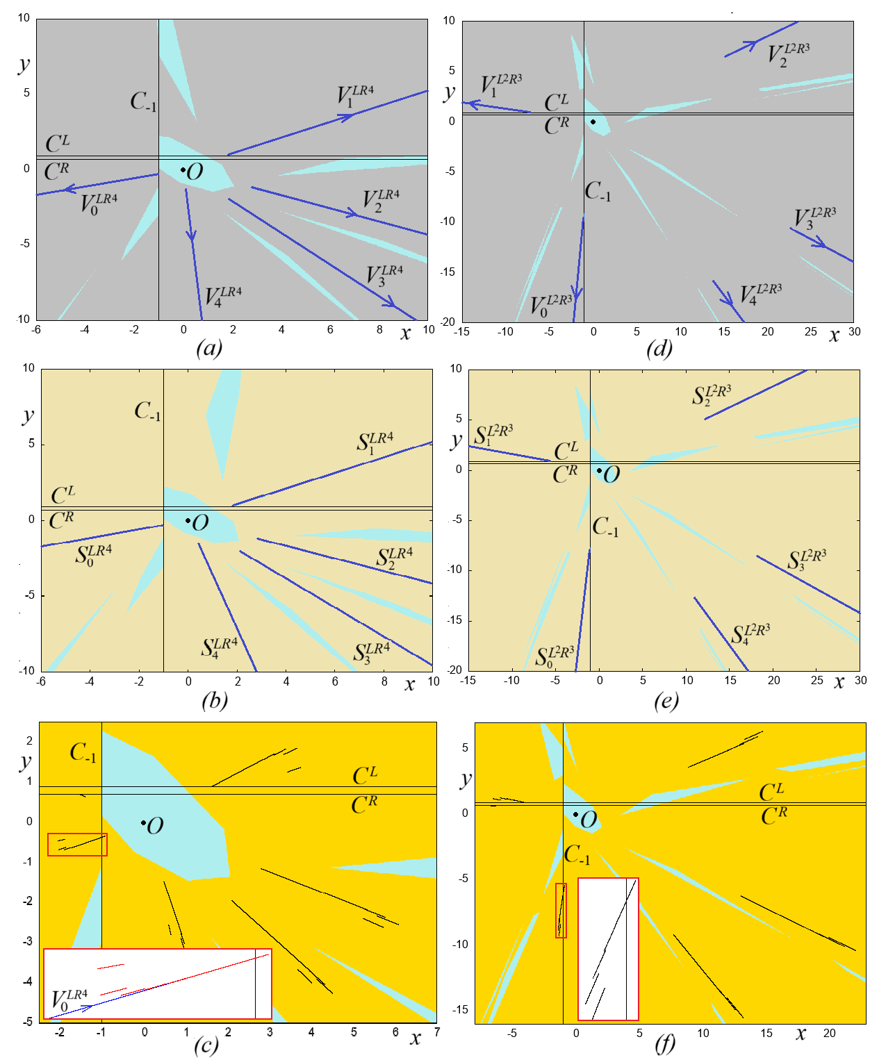
Figure 6: Phase portrait of map $F$ at $\delta_{L}=0.9,$ $\delta_{R}=0.7,$ $\tau_{L}=-2$ and (a) $\tau_{R}=1.1;$ (b) $\tau_{R}=1.15045;$ (c) $\tau_{R}=1.16;$ (d) $\tau_{R}=1.075;$ (e) $\tau_{R}=1.0719;$ (f) $\tau_{R}=1.067.$ The related parameter points are marked in Fig. 5 by $a$, $b$, …, $f$, respectively. The insets in (c) and (f) show the marked windows magnified.

$\bullet$ Let us now turn to the parameter point $d$ located above curve $B_{L^{2}R^{3}}$ but below curve $H_{LR^{4}}.$ The related phase portrait is shown in Fig. 6(d). In this case, the fixed point $O$ coexists with divergent trajectories; more precisely, it holds that $P_{L^{2}R^{3}}(1)<0$, that is, one eigenvalue of matrix $J_{L^{2}R^{3}}$ is larger than $1$, and the corresponding forward invariant repelling eigenvectors of map $F$ are located in the proper partitions: $V_{0,1}^{L^{2}R^{3}}\subset D_{L},$ $V_{j}^{L^{2}R^{3}}\subset D_{R},$ $j=\overline{2,4}$ (in Fig. 6(d), these eigenvectors are shown in dark blue).

The right column in Fig. 6 illustrates how the phase portrait of map $F$ changes for decreasing values of $\tau_{R}$ when the parameter point crosses boundary $B_{L^{2}R^{3}}.$

$\bullet$ Parameter point $e.$ Fig. 6(e) shows the related phase portrait. It holds that $(\tau_{L},\tau_{R})\in B_{L^{2}R^{3}}$, thus $P_{L^{2}R^{3}}(1)=0,$ and besides the attracting fixed point $O,$ there exists a set $S^{L^{3}R^{3}}$ consisting of $5$-cyclic halflines, $S_{0,1}^{L^{3}R^{3}}\subset D_{L}$ and $S_{j}^{L^{2}R^{3}}\subset D_{R},$ $j=\overline{2,4}$ ($S^{L^{3}R^{3}}=V_{j}^{L^{2}R^{3}}$), filled with nonhyperbolic $L^{2}R^{3}$-cycles (see Property 6);

$\bullet$ Parameter point $f.$ Fig. 6(f) presents the corresponding phase portrait. The parameter point $f$ is below $B_{L^{2}R^{3}}$, so that $P_{L^{2}R^{3}}(1)>0,$ and the attracting fixed point $O$ coexists with a WQA denoted $\mathcal{A}$, born after crossing boundary $B_{L^{2}R^{3}}$. The mechanism of its creation is similar to the one described in the previous example. Note that in this case, the parameter point is below curve $B_{L^{2}R^{3}}$ but above curve $E_{L^{2}R^{3}}$. Hence, the eigenvalues of matrix $J_{L^{2}R^{3}}$ are both real, positive, and less than $1$.

It is interesting to compare the WQAs shown in Figs. 6(c) and 6(f). Considering map $F^{5},$ it can be determined that the attractor in Fig. 6(f) consists of five cyclic blocks, unlike the attractor shown in Fig. 6(c), which is not cyclic. In fact, the complete block shown magnified in the inset in Fig. 6(f) is mapped in one block in partition $D_{L},$ while the block of the attractor shown magnified in the inset in Fig. 6(c) is mapped partially in $D_{L}$ and partially in $D_{R},$ breaking the cyclicity of this attractor.

$\bullet$ Parameter point $g$. This example is related to the case when the $(\tau_{L},\tau_{R})$-parameter point belongs to curve $B_{LR^{4}}.$ Since this point is below curve $H_{LR^{4}},$ the $LR^{4}$-cycle at infinity does not exist and curve $B_{LR^{4}}$ no longer serves as a boundary of the divergence region $D_{1/5}^{R}.$ However, an admissible set $S^{LR^{4}}$ still exists: it consists of five cyclic bounded segments, $S_{0}^{LR^{4}}\subset D_{L}$ and $S_{j}^{LR^{4}}\subset D_{R},$ $j=\overline{1,4},$ filled with nonhyperbolic $LR^{4}$-cycles. Figure 7(a) presents the phase portrait of map $F$, where the attracting fixed point $O$ coexists with segments $S_{j}^{LR^{4}},$ $j=\overline{0,4},$ shown in dark blue.

Starting from the case show in Fig. 7(a), a WQA denoted $\mathcal{A}$ appears for both increasing and decreasing values of $\tau_{R}$, as in Fig. 7(b) and Fig. 7(c), respectively. In particular, after crossing $B_{LR^{4}}$ for increasing $\tau_{R}$ (see Fig. 7(b)), eigenvectors $V_{j}^{LR^{4}}$ become attracting, so that segment $F^{5}(V_{0}^{LR^{4}})$ necessarily intersects the discontinuity line $C_{-1}$ and the mechanism of creation of attractor $\mathcal{A}$ is similar to the one illustrated in Figs. 6(b) and (c). Note that for further increasing $\tau_{R},$ attractor $\mathcal{A}$ disappears quite quickly due to a contact with the basin boundary of the fixed point $O$. In contrast, crossing $B_{LR^{4}}$ for decreasing $\tau_{R}$ (see Fig. 7(c)), eigenvectors $V_{j}^{LR^{4}}$ become repelling, so that segment $F^{5}(V_{4}^{LR^{4}})$ necessarily intersects the discontinuity line $C_{-1}$, and the mechanism of creation of a WQA is associated with further images of segment $F^{5}(V_{4}^{LR^{4}})|_{D_{L}}.$

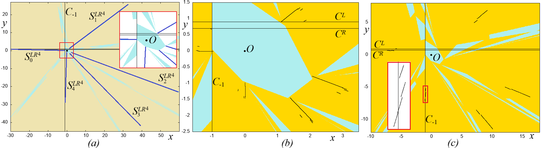
Figure 7: Phase portrait of map $F$ at $\delta_{L}=0.9,$ $\delta_{R}=0.7,$ $\tau_{L}=-1.125$ and (a) $\tau_{R}=1.04053,$ (b) $\tau_{R}=1.05$, (c) $\tau_{R}=1.02$. The parameter point related to (a) is marked in Fig. 5(a) by $g$. In (c), the inset shows the indicated window magnified.

4.2 Dynamics of map $F$ near the divergence region $D_{1/5}^{L}$

We now turn to an example of the bifurcation structure near the divergence region $D_{1/5}^{L}$. Figure 8(a) shows the $(\tau_{L},\tau_{R})$-parameter plane for $\delta_{L}=0.9,$ $\delta_{R}=0.7$, where besides curves $B_{RL^{4}}$ and $B_{R^{2}L^{3}},$ given in (16) and (18), also curves $H_{RL^{4}}$, $E_{RL^{4}},$ and $E_{R^{2}L^{3}},$ given in (20), (17), and (19), respectively, are shown. Comparing with the divergence region $D_{1/5}^{R}$ in Fig. 5(a), region $D_{1/5}^{L}$ in Fig. 8(a) is located not entirely in the stability domain of the fixed point $O,$ but also in the region below the straight line $\tau_{R}=-1.7,$ where the fixed point $O$ is a saddle. Figure 8(b) and its magnified part in the right panel present a 1D bifurcation diagram for $y$ versus $\tau_{L},$ setting $\tau_{R}=-2.$ The corresponding parameter path is indicated in Fig. 8(a) by the red horizontal segment. This diagram confirms, in particular, that attractors of map $F$ have no points in the strip between the critical lines $C^{R}$ and $C^{L}$ (zone $Z_{0}$ in Property 2(a)), defined in the considered case by $y=0.7$ and $y=0.9$, respectively (see two horizontal straight lines in Fig. 8(b)). Below, we give a few examples related to Fig. 8(b).

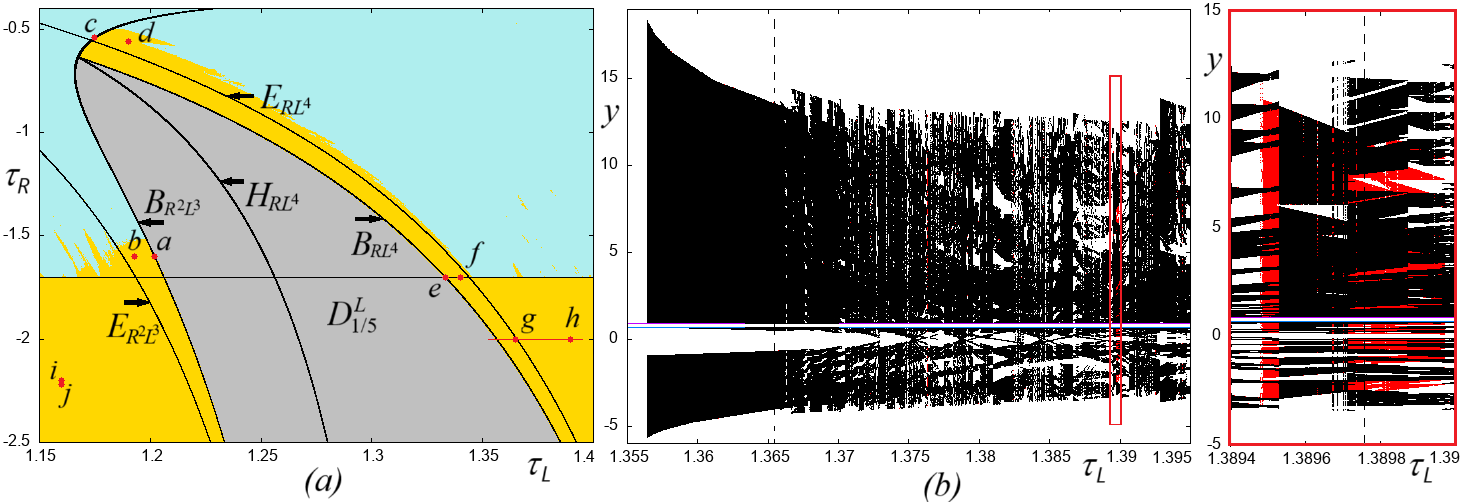
Figure 8: (a) The existence regions (in yellow) of the WQAs near the divergence region $D_{1/5}^{L}$ (in gray) bounded by curves $B_{RL^{4}}$ and $B_{R^{2}L^{3}}$ in the $(\tau_{L},\tau_{R})$-parameter plane for $\delta_{L}=0.9,$ $\delta_{R}=0.7;$ (b) 1D bifurcation diagram $y$ versus $\tau_{L}$ for $\tau_{R}=-2$. The rightmost figure presents a magnified window indicated in (b), where coexisting WQAs (shown in red and black) are better visible. The phase portraits of map $F$ at parameter points marked by $a,$ $b,$ …, $j$ are shown in Figs. 9(a),(b), 10(a),(b), 11(a),(b), 12(a),(b), and 13(a),(b), respectively.

To illustrate the dynamics of map $F$ near the divergence region $D_{1/5}^{L},$ we present the phase portraits of map $F$ for parameter values indicated in Fig. 8(a) by $a,$ $b,$ $c,$…, $j.$ The following should be noted:

$\bullet$ Parameter points $a$ and $b$. In Fig. 9(a), related to the parameter point $a$ belonging to curve $B_{R^{2}L^{3}}$, besides the attracting fixed point $O,$ there exists a set $S^{R^{2}L^{3}}$ consisting of five cyclic halflines, $S_{0,1}^{R^{2}L^{3}}\subset D_{R}$ and $S_{j}^{R^{2}L^{3}}\subset D_{L},$ $j=\overline{2,4}$ ($S_{j}^{R^{2}L^{3}}=V_{j}^{R^{2}L^{3}}$), filled with nonhyperbolic $R^{2}L^{3}$-cycles (see Property 6). Unlike crossing boundary $B_{RL^{4}}$, crossing boundary $B_{R^{2}L^{3}}$ may not lead to a WQA. In fact, after crossing $B_{RL^{4}},$ eigenvectors $V_{j}^{R^{2}L^{3}},$ $j=\overline{0,4},$ become attracting, thus after five iterations, halfline $F^{5}(V_{4}^{R^{2}L^{3}})$ and/or $F^{5}(V_{2}^{R^{2}L^{3}})$ necessarily intersects partition $D_{R}.$ It may happen that the segment(s) of $F^{5}(V_{4}^{R^{2}L^{3}})$ and/or $F^{5}(V_{2}^{R^{2}L^{3}})$ located in $D_{R}$ immediately after the bifurcation enter(s) the basin of the attracting fixed point $O,$ and thus no WQA appears. It can be seen in Fig. 9(a) that segments $S_{j}^{R^{2}L^{3}}$ are relatively far from the basin of the fixed point $O,$ and for decreasing $\tau_{L}$ a WQA, as, e.g., in Fig. 9(b), is created. Note that the related parameter point $b$ in Fig. 8(a) is located between curves $B_{R^{2}L^{3}}$ and $E_{R^{2}L^{3}},$ where the eigenvalues of the matrix $J_{R^{2}L^{3}}$ are both real, positive, and less than $1$.

Figure 9: Phase portrait of map $F$ at $\delta_{L}=0.9,$ $\delta_{R}=0.7,$ $\tau_{R}=-1.6$ and (a) $\tau_{L}=1.201945,$ (b) $\tau_{L}=1.193.$ In Fig. 8(a), the related parameter points are marked by $a$ and $b$, respectively.

$\bullet$ Parameter points $c$ and $d$. In Fig. 10(a), the phase portrait of map $F$ is shown for the parameter point $c$ belonging to curve $B_{R^{2}L^{3}}$. In contrast to the case in Fig. 9(a), the parameter point is above curve $H_{RL^{4}}.$ In this region, an $R^{2}L^{3}$-cycle at infinity does not exist, and this part of curve $B_{R^{2}L^{3}}$ is not at the boundary of the divergence region $D_{1/5}^{L}.$ However, an admissible set $S^{R^{2}L^{3}}$ still exists, consisting of five cyclic bounded segments, $S_{0,1}^{R^{2}L^{3}}\subset D_{R}$ and $S_{j}^{R^{2}L^{3}}\subset D_{L},$ $j=\overline{2,4}$ ($S_{j}^{R^{2}L^{3}}=V_{j}^{R^{2}L^{3}}$) filled with nonhyperbolic $R^{2}L^{3}$-cycles (see Property 6). An example of a WQA existing for the parameter values on the right of curve $B_{R^{2}L^{3}}$ is shown in Fig. 10(b). Note that the related parameter point $d$ in Fig. 8(a) belongs to the region where eigenvectors $V_{j}^{R^{2}L^{3}},$ $j=\overline{0,4},$ are repelling. Comparing with the example in Fig. 9, boundary $B_{R^{2}L^{3}}$ is crossed in the opposite direction: segment $F^{5}(V_{0}^{R^{2}L^{3}})$ necessarily intersects partition $D_{L}$ (see the inset in Fig. 10(b)). Further iterations of segment $F^{5}(V_{0}^{R^{2}L^{3}})|_{D_{L}}$ lead to new segments, and the WQA can be seen as a limit set of this process.

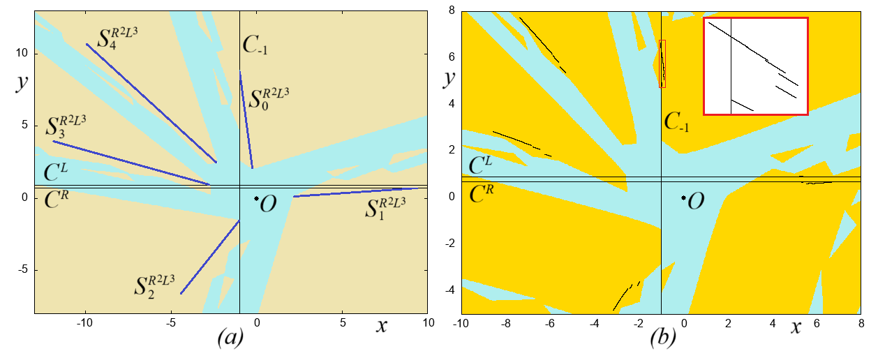
Figure 10: Phase portrait of map $F$ at $\delta_{L}=0.9,$ $\delta_{R}=0.7$ and (a) $\tau_{L}=1.175,$ $\tau_{R}=-0.543,$ (b) $\tau_{L}=1.19,$ $\tau_{R}=-0.56.$ In Fig. 8(a), the related parameter points are marked by $c$ and $d$, respectively.

$\bullet$ Parameter points $e$ and $f.$ In Fig. 11(a) a special case is illustrated where parameter point $e$ belongs to curve $B_{RL^{4}}$ and $\tau_{R}=-1.7$. Recall that at $\tau_{R}=-1.7,$ the fixed point $O$ undergoes a degenerate flip bifurcation (see Property 4): there is a segment $S^{R^{2}}=\{(x,y):-1<x<1,\ y=0.7x\}$ filled with points of nonhyperbolic $2$-cycles (except the fixed point $O$), and this segment coexists with a set $S^{RL^{4}}$ consisting of five cyclic halflines, $S_{0}^{RL^{4}}\subset D_{R}$ and $S_{j}^{RL^{4}}\subset D_{L},$ $j=\overline{1,4},$ filled with nonhyperbolic $RL^{4}$-cycles. An example of a WQA born on the right side of curve $B_{RL^{3}}$ and coexisting with segment $S^{R^{2}}$ is shown in Fig. 11(b). The related parameter point is marked $f$ in Fig. 8(a).

Figure 11: Phase portrait of map $F$ at $\delta_{L}=0.9,$ $\delta_{R}=0.7,$ $\tau_{R}=-1.7$ and (a) $\tau_{L}=1.333153,$ (b) $\tau_{L}=1.34.$ In Fig. 8(a), the related parameter points are marked by $e$ and $f$, respectively.

$\bullet$ Parameter points $g$ and $h$. In Fig. 12, two examples of the phase portrait of map $F$ are shown related to the 1D bifurcation diagram in Fig. 8(b). It is easy to verify that the WQA shown in Fig. 12(a) related to the parameter point $g$, consists of five cyclic blocks, that is, each block is $F^{5}$-invariant. In this case, only one block intersects the discontinuity line, and this entire block is mapped into the same partition $D_{R}.$ The cyclicity is not lost immediately but soon after crossing curve $E_{RL^{4}}$ (at $\tau_{L}\approx 1.36540484,$ see the dashed vertical line in Fig. 8(b)), when the eigenvalues of matrix $J_{RL^{4}}$ become complex-conjugate. Figure 12(b) related to the parameter point $h$, illustrates two coexisting WQAs and their basins at $\tau_{L}=1.38975$ (see the dashed vertical line in the right panel of Fig. 8(b)). As can be seen in the right panel of Fig. 8(b), there are several intervals of bistability, confirming that the coexistence of two WQAs may be persistent under parameter perturbations.

Figure 12: Phase portrait of map $F$ at $\delta_{L}=0.9,$ $\delta_{R}=0.7,$ $\tau_{R}=-2$ and (a) $\tau_{L}=1.365,$ (b) $\tau_{L}=1.38975.$ In Fig. 8(a), the related parameter points are marked by $g$ and $h$, respectively.

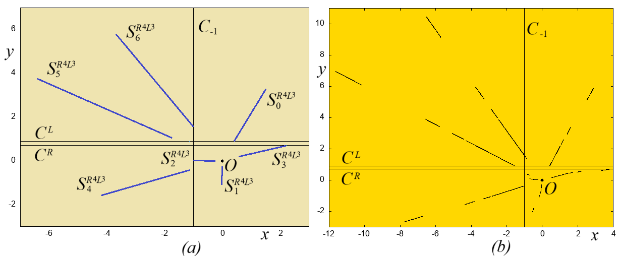
Figure 13: Phase portrait of map $F$ at $\delta_{L}=0.9,$ $\delta_{R}=0.7,$ $\tau_{L}=1.16$ and (a) $\tau_{R}=-2.199528,$ (b) $\tau_{L}=-2.219.$ In Fig. 8(a), the related parameter points are marked by $i$ and $j$, respectively.

$\bullet$ Parameter points $i$ and $j.$ Finally, it is worth noting that in the $(\tau_{L},\tau_{R})$-parameter plane in Fig. 8(a), there are parameter values associated with segments filled with nonhyperbolic cycles having symbolic sequences that are different from those considered above, i.e., from the basic and complementary symbolic sequences. An example is shown in Fig. 13(a), in the case when map $F$ has a set of seven cyclic segments $S_{j}^{R^{4}L^{3}},$ $j=\overline{0,6},$ filled with nonhyperbolic $R^{4}L^{3}$-cycles (the related point is marked $i$). A WQA appearing for decreasing $\tau_{R},$ e.g., at the parameter point $j$, is shown in Fig. 13(b). A mechanism of creation of this attractor is associated with segment $V_{6}^{R^{4}L^{3}}\subset D_{L},$ which now, after seven iterations, intersects the discontinuity line that leads to a new segment in $D_{R},$ whose images approach, as $n\rightarrow\infty,$ segments $V_{j}^{R^{4}L^{3}}.$ The WQA is a limit set of this process. This is not surprising, since we have shown only a few curves in the parameter space associated with $P_{\sigma}(1)=0,$ but clearly there are infinitely many such curves (although they all have zero Lebesgue measure), and they may be associated with the appearance of WQAs.

5 Conclusions

We considered a 2D piecewise linear map defined by two linear homogeneous functions in two partitions of the phase plane separated by a vertical discontinuity line. This map can have a new type of attractor, which we call a weird quasiperiodic attractor. This type of attractor was first observed in applied models (see, e.g., [17], [11], [13]). A WQA may consist of an infinite number of segments, fill some 2D subsets of the phase plane in a (seemingly) dense manner, or have a mixed structure. At first glance, a WQA may be misinterpreted as a chaotic attractor due to its intricate (weird) structure. However, chaos cannot be observed in the considered map since it cannot have hyperbolic cycles. The complex structure of the attractor is primarily related to the discontinuity of the map and the homogeneity of its linear components.

The present paper can be seen as a first step towards understanding the basic properties of WQAs and the mechanisms of their emergence. We described the bifurcation structure of the parameter space of map $F$ and analytically obtained some boundaries of the divergence regions, crossing which a WQA can appear. Special attention was paid to the case when map $F$ has $Z_{1}-Z_{0}-Z_{1}$ type of invertibility (an analog of a 1D gap map). To illustrate how a WQA can appear/disappear, we described in detail the corresponding transformations of the phase portrait of the map.

However, many issues remain unresolved. The first set of questions concerns the class of maps that can have WQAs. It is clear that this class includes discontinuous piecewise linear maps of dimension two or higher, defined by two or more homogeneous linear functions, or linear functions with the same fixed point (which can be translated to the origin, leading to the homogeneous case). It is also clear that discontinuity is a necessary element for the existence of a WQA. However, it remains an open problem whether linearity of the map components is a necessary condition or whether the functions defining the map can be nonlinear. There are also questions related to the structure of WQAs. For example, we conjecture that the structure of a WQA cannot be fractal, but it is not easy to prove this statement in the general case. One of the main questions is related to the quasiperiodicity of the trajectory on the attractor. It is well known that for the standard quasiperiodic attractor, such as an attracting closed invariant curve in the case of irrational rotation, the maximum Lyapunov exponent is zero, and there is no sensitive dependence on initial conditions. In the case of WQA, dependence on initial conditions is inevitable due to the discontinuity of the map. Taking two adjacent points belonging to the attractor but on opposite sides of the discontinuity line will necessarily lead to two images of these points that are distant from each other. In [17], this property is called weak sensitive dependence on initial conditions. The question is how weak this dependence is and whether the maximum Lyapunov exponent remains zero (numerically it is slightly positive, but we think this may be a numerical problem). It is also worth mentioning an interesting problem related to the mechanism of the emergence of WQAs and their properties when the map is noninvertible of $Z_{1}-Z_{2}-Z_{1}$ type. Some of the aforementioned problems are addressed in our companion paper [12], while others are left for further research.

Acknowledgements

Laura Gardini thanks the Czech Science Foundation (Project 22-28882S), the VSB—Technical University of Ostrava (SGS Research Project SP2024/047), the European Union (REFRESH Project-Research Excellence for Region Sustainability and High-Tech Industries of the European Just Transition Fund, Grant CZ.10.03.01/00/22 003/000004). Davide Radi thanks the Gruppo Nazionale di Fisica Matematica GNFM-INdAM for their financial support. The work of Davide Radi and Iryna Sushko was funded by the European Union - Next Generation EU, Mission 4: ”Education and Research” – Component 2: ”From research to business”, through PRIN 2022 under the Italian Ministry of University and Research (MUR). Project: 2022JRY7EF – Qnt4Green – Quantitative Approaches for Green Bond Market: Risk Assessment, Agency Problems and Policy Incentives - CUP: J53D23004700008.

References

- [1] V. Avrutin, L. Gardini, I. Sushko and F. Tramontana, Continuous and discontinuous piecewise-smooth one-dimensional maps: invariant sets and bifurcation structures. World Scientific, Singapore, 2019.
- [2] V. Avrutin, Zh.T. Zhusubaliyev, A. Saha, S. Banerjee, I. Sushko and L. Gardini, Dangerous Bifurcations Revisited, International Journal of Bifurcation and Chaos, Vol. 26, No. 14 (2016) 1630040 (24 pages).
- [3] A.F. Beardon, S.R. Bullett, and P.J. Rippon, Periodic orbits of difference equations, Proc. Roy. Soc. Edinburgh 125 (1995) 657–674.
- [4] M. di Bernardo, C.J. Budd, A.R. Champneys and P. Kowalczyk, Piecewise-Smooth Dynamical Systems: Theory and Applications, Appl. Math. Sci. 163, Springer, New York, 2008.
- [5] Y. Do and H.K. Baek, Dangerous border-collision bifurcations of a piecewise-smooth map, Commun. Pure Appl. Anal. 5, 493 (2006).
- [6] Y. Do, A mechanism for dangerous border collision bifurcations, Chaos Solit. Fract. 32 (2007) 352–362
- [7] J. Duan, Z. Wei, G. Li, D. Li and C. Grebogi, Strange nonchaotic attractors in a class of quasiperiodically forced piecewise smooth systems. Nonlinear Dyn 112 (2024) 12565–12577, https://doi.org/10.1007/s11071-024-09678-6
- [8] U. Feudel, S. Kuznetsov and A. Pikovsky, Strange nonchaotic attractors: dynamics between order and chaos in quasiperiodically forced systems. World Scientific. Singapore, 2006.
- [9] A. Ganguli and S. Banerjee, Dangerous bifurcation at border collision: When does it occur? Phys. Rev. E 71, 057202-1–057202-4, 2005.
- [10] L. Gardini, V. Avrutin and M. Schanz, Connection between bifurcations on the Poincarè equator and dangerous bifurcations, Iteration Theory, eds. Sharkovsky, A. and Sushko, I. (Grazer Math. Ber.) 53–72, 2009.
- [11] L. Gardini, D. Radi, N. Schmitt, I. Sushko and F. Westerhoff. On the limits of informationally efficient stock markets: New insights from a chartist-fundamentalist model, https://doi.org/10.48550/arXiv.2410.21198.
- [12] L. Gardini, D. Radi, N. Schmitt, I. Sushko and F. Westerhoff. Abundance of weird quasiperiodic attractors in PWL maps, Working Paper, University of Bamberg, 2025.
- [13] L. Gardini, D. Radi, N. Schmitt, I. Sushko and F. Westerhoff. How risk aversion may shape the dynamics of stock markets: a chartist-fundamentalist approach. Working Paper, University of Bamberg, 2025.
- [14] L.B. Garcia-Morato, E. Freire Macias, E. Ponce Nuñez and F. Torres Perat, Bifurcation patterns in homogeneous area-preserving piecewise-linear map, Qual. Theory Dyn. Syst. 18 (2019) 547–582.
- [15] C. Grebogi, E. Ott, S. Pelikan, and J.A. Yorke, Strange attractors that are not chaotic, Physica D 13 (1984) 261–268.
- [16] M.A. Hassouneh, E.H. Abed and H.E. Nusse, Robust dangerous border-collision bifurcations in piecewise smooth systems, Phys. Rev. Lett. 92 (2004) 070201.
- [17] L.E. Kollar, G. Stepan, and J. Turi, Dynamics of piecewise linear discontinuous maps. Int. J. Bif. Chaos, 14 (2004) 2341-2351.
- [18] J.C. Lagarias and E. Rains, Dynamics of a family of piecewise-linear area-preserving plane maps I. Rational rotation numbers, J. Difference Equ. Appl. 11 (2005) 1089–1108.
- [19] J.C. Lagarias and E. Rains, Dynamics of a family of piecewise-linear area-preserving plane maps II. Invariant circles, J. Difference Equ. Appl. 11 (2005) 1137–1163.
- [20] J.C. Lagarias and E. Rains, Dynamics of a family of piecewise-linear area-preserving plane maps III. Cantor set spectra, J. Differ. Equ. Appl. 11 (2005) 1205–1224.
- [21] C. Mira, L. Gardini, A. Barugola and J. C. Cathala, Chaotic Dynamics in Two-Dimensional Noninvertible Maps, World Scientific, Singapore, 1996.
- [22] H.E. Nusse and J.A. Yorke, Border-collision bifurcations including ‘period two to period three’ bifurcation for piecewise smooth systems, Physica D 57 (1992) 39–57.
- [23] J.A.G. Roberts, A. Saito and F. Vivaldi, Critical curves of rotations, Indagationes Mathematicae 35 (2024) 989–1008.
- [24] A. Sharkovsky, S. Kolyada, A. Sivak, and V. Fedorenko, Dynamics of One-dimensional Maps, Kluer Academic, Dorbrecht, 1997.
- [25] D. Simpson and J. Meiss, Neimark-Sacker bifurcations in planar, piecewise-smooth, continuous maps, SIAM J. Applied Dynamical Systems 7 (2008) 795–824.
- [26] D. Simpson, Bifurcations in Piecewise-Smooth Continuous Systems, World Scientific Series on Nonlinear Science, Vol. 70, World Scientific, Singapore, 2010.
- [27] D.J.W. Simpson, Border-Collision Bifurcations in , SIAM Review, 58, 2 (2016) 177–226.
- [28] D.J.W. Simpson, The Stability of Fixed Points on Switching Manifolds of Piecewise-Smooth Continuous Maps, Journal of Dynamics and Differential Equations 32 (2020) 1527–1552.
- [29] A.G. Sivak, Periodicity of Recursive Sequences and the Dynamics of Homogeneous Piecewise Linear Maps of the Plane, Journal of Difference Equations and Applications, Vol. 0 (2001) 1-24.
- [30] I. Sushko and L. Gardini, Center bifurcation for two-dimensional border-collision normal form, Int.J. Bifur. Chaos 18 (2008) 1029–1050.
- [31] I. Sushko and L. Gardini, Degenerate bifurcations and border collisions in piecewise smooth 1D and 2D maps, Int. J. Bifur. Chaos, 20 (2010) 2045–2070.
- [32] G. Li, Y. Yue, J. Xie, and C. Grebogi, Strange nonchaotic attractors in a nonsmooth dynamical system, Commun. Nonlinear Sci. Numer. Simul. 78 (2019) 104858.
- [33] G. Li, Y. Yue, J. Xie, and C. Grebogi, Multistability in a quasiperiodically forced piecewise smooth dynamical system, Commun. Nonlinear Sci. Numer. Simul. 84 (2020) 105165.
- [34] Zh T. Zhusubaliyev and E. Mosekilde, Bifurcations and Chaos in Piecewise-Smooth Dynamical Systems, World Sci. Ser. Nonlinear Sci. Ser. A Monogr. Treatises 44, World Scientific, Hackensack, NJ, 2003.