CRPS-Based Targeted Sequential Design with Application in Chemical Space

Abstract

Sequential design of real and computer experiments via Gaussian Process (GP) models has proven useful for parsimonious, goal-oriented data acquisition purposes. In this work, we focus on acquisition strategies for a GP model that needs to be accurate within a predefined range of the response of interest. Such an approach is useful in various fields including synthetic chemistry, where finding molecules with particular properties is essential for developing useful materials and effective medications. GP modeling and sequential design of experiments have been successfully applied to a plethora of domains, including molecule research. Our main contribution here is to use the threshold-weighted Continuous Ranked Probability Score (CRPS) as a basic building block for acquisition functions employed within sequential design. We study pointwise and integral criteria relying on two different weighting measures and benchmark them against competitors, demonstrating improved performance with respect to considered goals. The resulting acquisition strategies are applicable to a wide range of fields and pave the way to further developing sequential design relying on scoring rules.

Keywords: Active Learning, Excursion Set Estimation, Gaussian Processes, Scoring Rules, Stepwise Uncertainty Reduction, Uncertainty Quantification

1 Introduction

Gaussian Process (GP) modeling, originating from the geostatistical interpolation method known as kriging (Krige,, 1951), extends its application beyond geostatistics (Rasmussen and Williams,, 2006). Its fundamental concept revolves around modeling a target function $f:\mathcal{X}\rightarrow\mathbb{R}$ from a set of input locations $\mathcal{X}$ to the real numbers; in the case of co-kriging or multitask GP models, the function can also produce vector-valued outputs. Given a finite number of evaluations of $f$ or of by-products thereof (e.g., evaluations of derivatives of $f$), the objective is typically to predict $f$ at arbitrary locations. GP modeling is favored for its suitability with a limited amount of training data, provision of a full predictive distribution enabling uncertainty quantification, and capability to also handle non-Euclidean inputs through appropriate covariance kernels. In terms of the latter, the selection of kernels can be tailored to specific data types and applications. In scenarios where data collection is resource-intensive, efficiently selecting and expanding the training dataset is crucial. In this context, we employ targeted sequential design strategies, with a focus on an excursion set of the form $\Gamma:=\{x\in\mathcal{X}:f(x)\geq t\}$, using some prescribed thereshold $t\in\mathbb{R}$. In doing so, we follow the now established framework of GP-based excursion set estimation (e.g., French and Sain,, 2013; Chevalier et al., 2013a, ; Bolin and Lindgren,, 2015; Azzimonti,, 2016, and references therein) and focus on two interconnected elements: suitable evaluation metrics and targeted acquisition criteria.

Scoring rules (Gneiting and Raftery,, 2007) are widely used tools for assessing probabilistic forecasts by comparing a predictive distribution with a single value (the materialized response). Scoring rules evaluate both the statistical consistency between predictions and observations (calibration) and the sharpness of the prediction. An interesting category of scoring rules for goal-oriented prediction evaluation consists of weighted scoring rules, allowing to emphasize particular outcomes by incorporating a weighting measure (Gneiting and Ranjan,, 2011). In this study, we focus on the Continuous Ranked Probability Score (CRPS; Matheson and Winkler, 1976), for which Allen et al., 2023b outline three potential approaches to use a weighting measure. Here, we consider the threshold-weighted CRPS introduced by Matheson and Winkler, (1976) and Gneiting and Ranjan, (2011), which has been widely used for evaluating forecasts of extreme weather events (e.g., Lerch and Thorarinsdottir,, 2013). To reflect the special importance of predictions in/near the excursion set $\Gamma$, we consider both an indicator weight on $\Gamma$, and a Gaussian weight centered at $t$.

In terms of data acquisition, we aim to extend the training set by strategically adding promising candidates, thereby improving the model with respect to our goals. While in the field of Bayesian global optimization (Kushner,, 1964; Močkus et al.,, 1978; Močkus,, 1989), the focus is on finding the optimum or an optimizer of $f$, we are focusing on the excursion set $\Gamma$. We rely on a sequential design strategy with selecting each training point as if it were the final one, known as a one-step look-ahead (or myopic) strategy. There exist different criteria to choose the next point, depending on the objective of interest. For a focus on the excursion set $\Gamma$, we distinguish between pointwise criteria, and integral criteria. Pointwise criteria focus solely on local GP predictions, with popular examples including the Targeted Mean Square Error (TMSE; Picheny et al., 2010) and entropy-based criteria (Cole et al.,, 2023). Integral criteria consider the predictive distribution over the entire domain $\mathcal{X}$ and well-known approaches include the Targeted Integrated Mean Square Error (TIMSE; Picheny et al.,, 2010) and Stepwise Uncertainty Reduction (SUR; Bect et al., 2012) criteria such as the Integrated Bernoulli Variance (IBV; Bect et al.,, 2019).

Given that the threshold-weighted CRPS, with an appropriate weighting measure, evaluates the GP model’s performance while emphasizing excursions, it also provides a promising foundation for designing targeted acquisition criteria. However, in their original form, scoring rules compare the prediction with the materialized response, which is unavailable during data acquisition. Yet, one may rely on the expected scoring rule by integrating the score of forecasting $y$ by $F$ under the assumption that $y$ is random with distribution $F$. This is also known as the entropy function of the score (Gneiting and Raftery,, 2007). The main contribution of this paper is the introduction and development of new pointwise and SUR data acquisition criteria based on the expected threshold-weighted CRPS. The CRPS has already been used in the realm of GP modeling; however, to the best of our knowledge, its application has been limited to parameter selection (e.g., Petit et al.,, 2023).

We showcase and compare the derived criteria and resulting sequential strategies on chemical test cases revolving around the Photoswitch dataset (Thawani et al.,, 2020). GP models have demonstrated indeed promising results in predicting molecular properties, as highlighted for instance in the work of Thawani et al., (2020), Deringer et al., (2021) and Griffiths et al., (2023). Thereby, the choice of kernel heavily depends on the molecule representation used to encode chemical structures. We consider molecules represented by molecular fingerprints (Christie et al.,, 1993; Johnson and Maggiora,, 1990), which encode the presence or absence of characteristic substructures using binary digits. For fingerprint representations, the Tanimoto kernel (Gower,, 1971) is widely utilized (e.g., Ralaivola et al.,, 2005; Miyao and Funatsu,, 2019; Tripp et al.,, 2023), favored due to its simplicity, efficiency, and effectiveness in measuring the overlap between the presence or absence of molecular features. By combining the Tanimoto kernel with our targeted CRPS-based criteria, we demonstrate how scoring rules can be leveraged for efficient sequential design towards uncovering molecules of interest.

The structure of the remaining paper is as follows: Section 2 reviews the fundamentals of GP modeling, excursion set estimation and targeted sequential design. While Section 3 is dedicated to the threshold-weighted CRPS and the development of the acquisition criteria based thereon, the numerical tests are introduced in Section 4 and the results are presented in Section 5. Section 6 wraps up the main body with a discussion and concluding words.

2 Gaussian Process Modeling and Sequential Design

2.1 Gaussian process modeling and excursion set estimation

Gaussian Processes (GPs) provide a flexible probabilistic framework for modeling unknown functions. A GP $\boldsymbol{\xi}=\left(\xi(\boldsymbol{x})\right)_{\boldsymbol{x}\in\mathcal{X}}$ is a collection of real-valued random variables $\xi(\boldsymbol{x})$ defined on a common probability space, such that for any finite subset $\{\boldsymbol{x}_{1},\dots,\boldsymbol{x}_{n}\}\subset\mathcal{X}$ with $n\geq 1$, the random vector $(\xi(\boldsymbol{x}_{1}),\dots,\xi(\boldsymbol{x}_{n}))$ follows a multivariate Gaussian distribution. The distribution of a GP is characterized by its mean $m:\mathcal{X}\to\mathbb{R}$, $m(\boldsymbol{x}):=\mathbb{E}[\xi(\boldsymbol{x})]$ and covariance function $k:\mathcal{X}\times\mathcal{X}\to\mathbb{R}$, $k(\boldsymbol{x},\boldsymbol{x}^{\prime}):=Cov(\xi(\boldsymbol{x}),\xi(\boldsymbol{x^{\prime}}))$.

In GP modeling, an unknown function $f:\mathcal{X}\rightarrow\mathbb{R}$ is assumed to be a realization of a GP $\boldsymbol{\xi}$. Here, we assume we observe noisy evaluations of $f$ at $n$ input locations $\{\boldsymbol{x}_{1},\dots,\boldsymbol{x}_{n}\}\subset\mathcal{X}$, yielding the observations: $Z_{i}=f(\boldsymbol{x_{i}})+\varepsilon_{i},\ \text{where }\varepsilon_{i}\sim\mathcal{N}(0,\tau^{2})\ \text{i.i.d.}$. Conditioning the GP on the observation event denoted as $\mathcal{A}_{n}=\{\boldsymbol{Z}_{n}=\boldsymbol{z}_{n}\}$ results in a posterior Gaussian distribution characterized by its predictive mean $m_{n}(\boldsymbol{x})$ and posterior covariance function $k_{n}(\boldsymbol{x},\boldsymbol{x^{\prime}})$, whose expressions are recalled in Appendix A.1.

A key advantage of GPs in our context is their ability to support the analysis of excursion sets of the form $\Gamma:=\{\boldsymbol{x}\in\mathcal{X}:f(x)\geq t\}$, where $t\in\mathbb{R}$ is prescribed. Indeed, we can compute the excursion probability at any location $\boldsymbol{x}\in\mathcal{X}$ in closed form:

$$p_{n}(\boldsymbol{x})=\mathbb{P}\left(\xi_{n}(\boldsymbol{x})\geq t\right)=\mathbb{P}\left(\frac{\xi_{n}(\boldsymbol{x})-m_{n}(\boldsymbol{x})}{\sqrt{k_{n}(\boldsymbol{x},\boldsymbol{x})}}\geq\frac{t-m_{n}(\boldsymbol{x})}{\sqrt{k_{n}(\boldsymbol{x},\boldsymbol{x})}}\right)=\Phi\left(\frac{m_{n}(\boldsymbol{x})-t}{\sqrt{k_{n}(\boldsymbol{x},\boldsymbol{x})}}\right),$$ (1)

where $\Phi(\cdot)$ is the CDF of the univariate standard Gaussian distribution.

The excursion probability can be utilized for classification purposes (Bect et al.,, 2012). Considering a hard classifier $\eta_{n}:\mathcal{X}\rightarrow\{0,1\}$, we denote the probability of misclassifications by $\tau_{n}(\boldsymbol{x})=\mathbb{P}(\eta_{n}(\boldsymbol{x})\neq\mathbbm{1}\{\xi(\boldsymbol{x})\geq t\})$. It holds that $\tau_{n}(\boldsymbol{x})=p_{n}(\boldsymbol{x})+(1-2p_{n}(\boldsymbol{x}))\eta_{n}(\boldsymbol{x})$, which is minimized if $\eta_{n}(\boldsymbol{x})=\mathbbm{1}\{p_{n}(\boldsymbol{x})\geq 0.5\}$. Using this classifier, we thus arrive at the following estimator for the excursion set (Bect et al.,, 2012):

$$\hat{\Gamma}:=\{\boldsymbol{x}\in\mathcal{X}:p_{n}(\boldsymbol{x})\geq 0.5\}=\{\boldsymbol{x}\in\mathcal{X}:m_{n}(\boldsymbol{x})\geq t\}.$$ (2)

Depending on the specific objectives of the application, an alternative threshold than $0.5$ might be of interest. If sensitivity is prioritized, a threshold below $0.5$ might be of interest, such that more locations are classified as in the excursion set. Conversely, raising it above $0.5$ shifts the focus on specificity, leading to a more conservative classification (Azzimonti et al.,, 2019).

GP-based excursion set estimation extends beyond binary classification. The full probabilistic predictions provide richer information, including uncertainty quantification, and can be leveraged in various ways. In particular, this uncertainty can guide active learning strategies through targeted sequential design, ensuring that new evaluations refine the GP model with respect to the excursion set. Additionally, it can be incorporated into scoring-based approaches to evaluate, and ultimately improve, predictions.

2.2 Targeted Sequential Design

To refine the GP model with a focus on the excursion set, it is essential to carefully choose added training points. We consider one-step look-ahead (or myopic) strategies, which rely on a similar basic brick: from the ‘current’ conditional distribution of $\boldsymbol{\xi_{n}}$ given $\mathcal{A}_{n}$ based on the initial $n$ training points, choose the next point $\boldsymbol{x_{n+1}}$ by optimizing a selection criterion, a.k.a. acquisition function. Subsequently, the noise-contaminated $Z_{n+1}$ is collected and $\mathcal{A}_{n}$ is augmented into $\mathcal{A}_{n+1}$, leading to an update of the GP to $\boldsymbol{\xi_{n+1}}$. There exist a variety of selection criteria for sequential design; we distinguish between pointwise and SUR criteria.

Pointwise selection criteria

Given a GP $\boldsymbol{\xi_{n}}=\left(\xi_{n}(\boldsymbol{x})\right)_{\boldsymbol{x}\in\mathcal{X}}$, a pointwise selection criterion considers the marginal distributions and selects the next acquisition point $\boldsymbol{x}_{n+1}\in\mathcal{X}$ by maximizing

$$\boldsymbol{x}\mapsto G_{n}(\boldsymbol{x})=\mathcal{G}(\xi_{n}(\boldsymbol{x})),$$ (3)

where $\mathcal{G}(\cdot)$ maps the marginal Gaussian $\xi_{n}(\boldsymbol{x})\sim\mathcal{N}(m_{n}(\boldsymbol{x}),k_{n}(\boldsymbol{x},\boldsymbol{x}))$ to a real value. A very simplistic approach would be to consider the variance $G_{n}(\boldsymbol{x})=k_{n}(\boldsymbol{x},\boldsymbol{x})$ of all candidate points $\boldsymbol{x}\in\mathcal{X}$ and select one with highest variance as $\boldsymbol{x_{n+1}}$. For targeted sequential design focused on the excursion set $\Gamma$ , the objective is to define a local criterion that balances the trade-off between proximity to $\Gamma$ and high predictive uncertainty (Chevalier et al.,, 2014, Sections 3.2 and 4.5).

SUR selection criteria

Stepwise Uncertainty Reduction (SUR; Bect et al., 2019) criteria build upon notions of uncertainty that may involve the GP model on the entire domain rather than at a single point, and consider how such a measure of uncertainty evolves at time $n+1$ if the next evaluation is conducted at $\boldsymbol{x_{n+1}}=\boldsymbol{x}$. Given a GP model $\boldsymbol{\xi_{n}}$ at time $n$, a SUR criterion selects the next acquisition point by minimizing:

$$\boldsymbol{x}\mapsto J_{n}(\boldsymbol{x})=\mathbb{E}_{n,\boldsymbol{x}}[\mathcal{H}(\boldsymbol{\xi}_{n+1})],$$ (4)

where $\boldsymbol{\xi}_{n+1}\sim\mathrm{GP}(m_{n+1},k_{n+1})$ is the future GP conditioned on $\mathcal{A}_{n+1}$. Here $\mathcal{H}(\cdot)$ stands for an uncertainty functional that maps the whole (updated) GP model to a real-valued variable that summarizes the remaining uncertainty. Furthermore, $\mathbb{E}_{n,\boldsymbol{x}}(\cdot)$ denotes the conditional expectation with respect to $\boldsymbol{\xi_{n}}$ when $\boldsymbol{x_{n+1}}=\boldsymbol{x}$. For a simplistic acquisition approach based on variance, we could employ the integrated future variance $J_{n}(\boldsymbol{x})=\int k_{n+1}(\boldsymbol{x^{\prime}},\boldsymbol{x^{\prime}})\mathbb{P}_{\mathcal{X}}(\mathrm{d}\boldsymbol{x^{\prime}})$. SUR criteria targeting response-dependent regions are discussed in Sections 3.3 and 4.5.

3 Threshold-weighted CRPS for Sequential Design

3.1 Threshold-weighted CRPS

Scoring rules (Gneiting and Raftery,, 2007) provide a tool for evaluating probabilistic forecasts by measuring the alignment between a predictive distribution and the materialized value. One very popular scoring rule is the Continuous Ranked Probability Score (CRPS; Matheson and Winkler,, 1976), which for a predictive distribution with CDF $F(\cdot)$ and a materialized value $y$ is defined as,

$$\mathrm{CRPS}(F,y)=\int_{-\infty}^{\infty}[F(u)-\mathbbm{1}\{y\leq u\}]^{2}\,\mathrm{d}u.$$ (5)

In GP modeling, we would like to evaluate the performance of $\xi_{n}(\boldsymbol{x^{\prime}})\sim\mathcal{N}\left(m_{n}(\boldsymbol{x^{\prime}}),k_{n}(\boldsymbol{x^{\prime}},\boldsymbol{x^{\prime}})\right)$ in point $\boldsymbol{x^{\prime}}\in\mathcal{X}$ with respect to $f(\boldsymbol{x^{\prime}})$. We only consider one point $\boldsymbol{x^{\prime}}$ at a time (univariate), for which we use $\Phi_{\mu,\sigma^{2}}$ to denote the Gaussian predictive distribution with mean $\mu=m_{n}(\boldsymbol{x^{\prime}})$ and variance $\sigma^{2}=k_{n}(\boldsymbol{x^{\prime},\boldsymbol{x^{\prime}}})$. As in the traditional setting, we use $y=f(\boldsymbol{x^{\prime}})$ to denote the materialized value. In this setting, the CRPS writes as (Gneiting and Raftery,, 2007),

$$\mathrm{CRPS}\left(\Phi_{\mu,\sigma^{2}},y\right)=\sigma\left[\widetilde{y}\left(2\Phi\left(\widetilde{y}\right)-1\right)+2\phi\left(\widetilde{y}\right)-\frac{1}{\sqrt{\pi}},\right].$$ (6)

using $\widetilde{y}=(y-\mu)/\sigma$. The CRPS is negatively oriented, meaning that better predictions correspond to lower scores.

Weighted scoring rules enable a targeted assessment of forecasts. The threshold-weighted CRPS (Matheson and Winkler,, 1976; Gneiting and Ranjan,, 2011) extends the CRPS by considering a weighting measure $\nu$, which emphasizes the values of interest:

$$\mathrm{CRPS}_{\nu}(F,y)=\int_{-\infty}^{\infty}[F(u)-\mathbbm{1}\{y\leq u\}]^{2}\,\mathrm{d}\nu(u).$$ (7)

While $\nu$ may potentially be taken as any Borel measure on $\mathbb{R}$, in our excursion setting, we consider two types of weighting measures (characterized by their densities with respect to the Lebesgue measure $\lambda$). The first weighting measure $\nu_{1}$ only considers values above the threshold $t$ and is characterized by $\mathrm{d}\nu_{1}(u)=\mathbbm{1}\{t\leq u\}\mathrm{d}\lambda(u)$. The second weighting measure $\nu_{2}$ admits a Gaussian probability density centered on the threshold $t$ and with variance $\sigma_{\nu}^{2}>0$: $\mathrm{d}\nu_{2}(u)=\frac{1}{\sigma_{\nu}}\phi\left(\frac{u-t}{\sigma_{\nu}}\right)\mathrm{d}\lambda(u)$, where $\phi:\mathbb{R}\rightarrow(0,\infty),\phi(v):=\frac{1}{\sqrt{2\pi}}\exp^{-\frac{v^{2}}{2}}$.

Theorem 1.

For a predictive distribution $\Phi_{\mu,\sigma^{2}}$, it holds with weighting measure $\nu_{1}$ that

$$\mathrm{CRPS}_{\nu_{1}}(\Phi_{\mu,\sigma^{2}},y)=\sigma\left[-\widetilde{t}\Phi(\widetilde{t})^{2}+\widetilde{y^{t}}\left(2\Phi(\widetilde{y^{t}})-1\right)+\left(2\phi\left(\widetilde{y^{t}}\right)-2\phi\left(\widetilde{t}\right)\Phi(\widetilde{t})\right)-\frac{1}{\sqrt{\pi}}\left(1-\Phi(\widetilde{t}\sqrt{2})\right)\right],$$

where $\widetilde{t}=(t-\mu)/\sigma$ and $\widetilde{y^{t}}=\Big{(}\max(y,t)-\mu\Big{)}/\sigma$.

For the weighting measure $\nu_{2}$ (with mean $t$ and variance $\sigma_{\nu}^{2}$), one obtains

$$\mathrm{CRPS}_{\nu_{2}}(\Phi_{\mu,\sigma^{2}},y) =\Phi\left(\begin{pmatrix}0\\ 0\end{pmatrix};\begin{pmatrix}\mu-t\\ \mu-t\end{pmatrix},\begin{pmatrix}\sigma_{\nu}^{2}+\sigma^{2}&\sigma_{\nu}^{2}\\ \sigma_{\nu}^{2}&\sigma_{\nu}^{2}+\sigma^{2}\end{pmatrix}\right)$$

$$\quad\quad-2\Phi\left(\begin{pmatrix}0\\ 0\end{pmatrix};\begin{pmatrix}\mu-t\\ y-t\end{pmatrix},\begin{pmatrix}\sigma_{\nu}^{2}+\sigma^{2}&\sigma_{\nu}^{2}\\ \sigma_{\nu}^{2}&\sigma_{\nu}^{2}\end{pmatrix}\right)+\Phi\left(\frac{t-y}{\sigma_{\nu}}\right),$$

where $\Phi(\cdot;\boldsymbol{\mu},\boldsymbol{\Sigma})$ is the bivariate Gaussian CDF with parameters $\boldsymbol{\mu}\in\mathbb{R}^{2}$ and $\boldsymbol{\Sigma}\in\mathbb{R}^{2\times 2}$.

Proof.

See Appendix A.3.1. ∎

For illustration purposes, Figure 1 depicts the discussed versions of the CRPS for a Gaussian $\Phi_{\mu,\sigma^{2}}$ (black solid line), showing the area under the integral for the CRPS (a and d), $\mathrm{CRPS}_{\nu_{1}}$ (b and e), and $\mathrm{CRPS}_{\nu_{2}}$ (c and f) across two scenarios: In the first row (a-c) we consider $y<t<\mu$, referring to a point which does not lie in the excursion set ($y<t$), but is falsely predicted to be in the excursion set ($\mu>t$, see Eq. 2). In the second row (d-f), we use $\mu<t<y$, such that the point does lie in the excursion set ($y>t$), but is falsely predicted to be not ($\mu<t$). Notably, both the (unweighted) CRPS and $\mathrm{CRPS}_{\nu_{2}}$ are symmetric, yielding the same value for both scenarios. Contrarily, the $\mathrm{CRPS}_{\nu_{1}}$ has a higher value in the second scenario.

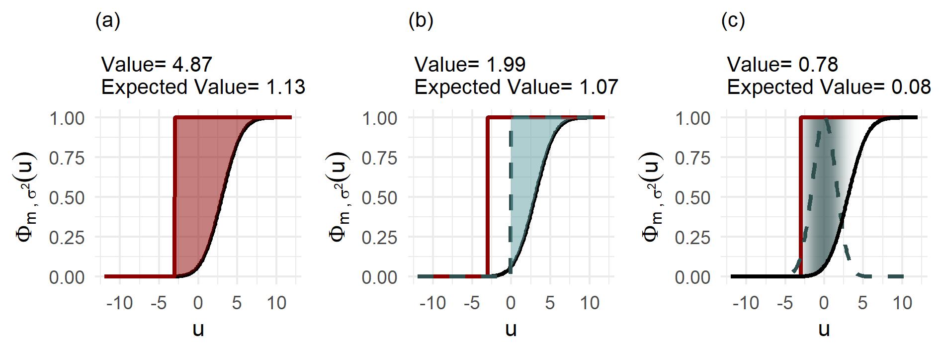
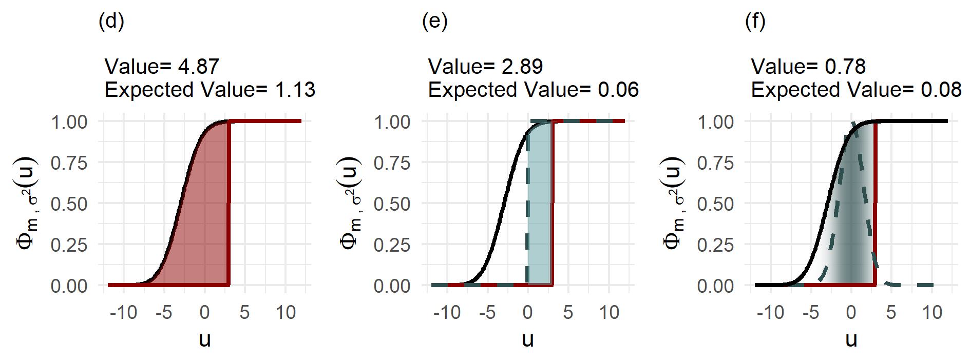
Figure 1: Illustrations of the $\mathrm{CRPS}\left(\Phi_{\mu,\sigma^{2}},y\right)$ and $\mathrm{CRPS}_{\nu}\left(\Phi_{\mu,\sigma^{2}},y\right)$ for a Gaussian CDF $\Phi_{\mu,\sigma^{2}}(u)$ (black solid line), an observation $y$ (solid indicator line) and a threshold $t$. In the first row (a-c) we have $y=-3,t=0,\mu=3$ and in the second row (d-f) we have $\mu=-3,t=0,y=3$; we use $\sigma=2$ for the predictive Gaussian. The individual plots display the area under the integral for the CRPS (a and d), $\mathrm{CRPS}_{\nu_{1}}$ (b and e) and $\mathrm{CRPS}_{\nu_{2}}$ (c and f; $\sigma_{\nu}=1.5$), with the dashed lines indicating the weighting measures $\nu_{1}$ and $\nu_{2}$. The numbers refer to the value and expected value of the respective criterion.

3.2 Pointwise selection criteria

Given that the threshold-weighted CRPS evaluates both accuracy and uncertainty of the GP model with respect to the excursion set of interest, it is a promising basis for an acquisition criterion. For a pointwise criterion, we consider the threshold-weighted CRPS of all the candidate points, and add the one to the training set which has the highest score (Eq. 3). However, in its original form for evaluation (Eq. 7), the threshold-weighted CRPS relies on the materialized value $y$ in the candidate point, which is unavailable during data acquisition. Therefore, we consider an expected version, where the expectation is taken with respect to the current predictive distribution. This is also known as the expected score or entropy function for proper scoring rules (Gneiting and Raftery,, 2007). The expected threshold-weighted CRPS with weighting measure $\nu$ for predictive CDF $F$ is defined as,

$$\mathrm{CRPS}_{\nu}(F)=\int_{-\infty}^{\infty}\mathrm{CRPS}_{\nu}(F,y^{\prime})\mathrm{d}F(y^{\prime}).$$ (8)

The following theorem provides an alternative representation of this expected threshold-weighted CRPS and derives explicit formulas for Gaussian predictive distributions with weighting measures $\nu_{1}$ and $\nu_{2}$.

Theorem 2.

For a predictive CDF $F(\cdot)$ and a weighting measure $\nu$, it holds,

$$\mathrm{CRPS}_{\nu}(F)=\int F(u)\left(1-F(u)\right)\mathrm{d}\nu(u).$$

Particularly, for $F=\Phi_{\mu,\sigma^{2}}$ and $\mathrm{d}\nu_{1}(u)=\mathbbm{1}\{t\leq u\}\mathrm{d}\lambda(u)$, one obtains,

$$\mathrm{CRPS}_{\nu_{1}}(\Phi_{\mu,\sigma^{2}})=\sigma\Big{[}\widetilde{t}\Phi(\widetilde{t})^{2}-\widetilde{t}\Phi(\widetilde{t})+\frac{1}{\sqrt{\pi}}-\frac{1}{\sqrt{\pi}}\Phi(\widetilde{t}\sqrt{2})+2\phi(\widetilde{t})\Phi(\widetilde{t})-\phi(\widetilde{t})\Big{]},$$

with $\widetilde{t}=(t-\mu)/\sigma$. An alternative representation is,

$$\mathrm{CRPS}_{\nu_{1}}(\Phi_{\mu,\sigma^{2}})=\sigma\mathbb{E}\left[\left(\widetilde{N}-\max\left(N,\frac{t-\mu}{\sigma}\right)\right)_{+}\right],$$

for $N,\widetilde{N}\overset{i.i.d.}{\sim}\mathcal{N}(0,1)$. For $\mathrm{d}\nu_{2}(u)=\frac{1}{\sigma_{\nu}}\phi\left(\frac{u-t}{\sigma_{\nu}}\right)\mathrm{d}\lambda(u)$, we get,

$$\mathrm{CRPS}_{\nu_{2}}(\Phi_{\mu,\sigma^{2}}) =\Phi\left(\begin{pmatrix}0\\ 0\end{pmatrix};\begin{pmatrix}\mu-t\\ t-\mu\end{pmatrix},\begin{pmatrix}\sigma_{\nu}^{2}+\sigma^{2}&-\sigma_{\nu}^{2}\\ -\sigma_{\nu}^{2}&\sigma_{\nu}^{2}+\sigma^{2}\end{pmatrix}\right).$$

Proof.

Appendix A.3.2; the first result generalizes the corresponding expression for the traditional CRPS (Gneiting and Raftery,, 2007). ∎

To use this for pointwise selection criteria (Eq. 3), we can set $G_{n}(\boldsymbol{x})=\mathrm{CRPS}_{\nu}(\Phi_{\mu,\sigma^{2}})$, where $\mu=m_{n}(\boldsymbol{x})$ and $\sigma^{2}=k_{n}(\boldsymbol{x,\boldsymbol{x}})$. To better understand the resulting behavior, we return to Figure 1, in which we also denote the expected score values. Both CRPS and $\mathrm{CRPS}_{\nu_{2}}$ maintain symmetry in their expected scores (a, c, d, f), while $\mathrm{CRPS}_{\nu_{1}}$ remains asymmetric but with a reversed orientation. In the original scoring rule relying on $y$, a missed point within the excursion set results in a higher score. In the expected score, a point mistakenly classified as being within the excursion set yields a higher expected score. In general, the $\mathrm{CRPS}_{\nu_{1}}$ is higher for cases where $\Phi_{\mu,\sigma^{2}}$ has $m>t$, regardless of whether the prediction is correct (since the correct outcome is unknown). Figure 2a shows this relationship for $\Phi_{\mu,\sigma^{2}}$ with a fixed $t=0$. Both the values of $\mathrm{CRPS}_{\nu_{1}}$ and $\mathrm{CRPS}_{\nu_{2}}$ increase with higher uncertainty ($\sigma$) for the same $\mu$. However, while $\mathrm{CRPS}_{\nu_{1}}$ continuously increases with rising $\mu$ when $\sigma$ is fixed, $\mathrm{CRPS}_{\nu_{2}}$ remains symmetric around the threshold $t$ for varying $\mu$.

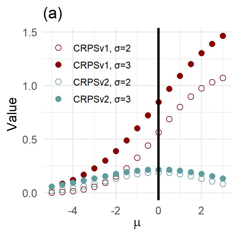
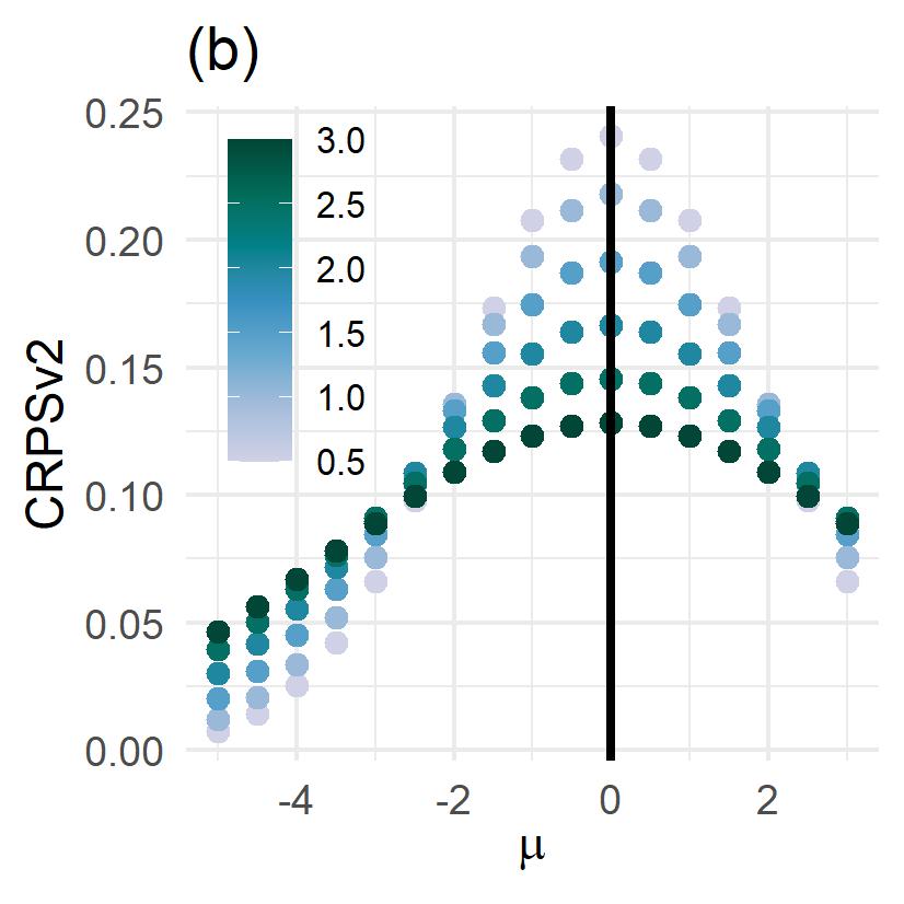
Figure 2: Illustrations of the expected $\mathrm{CRPS}_{\nu_{1}}$ and $\mathrm{CRPS}_{\nu_{2}}$ for a Gaussian $\Phi_{\mu,\sigma^{2}}$ depending on the predictive mean $\mu$: (a) Expected $\mathrm{CRPS}_{\nu_{1}}$ and $\mathrm{CRPS}_{\nu_{2}}$ ($\sigma_{\nu}=1.5$) and (b) Expected $\mathrm{CRPS}_{\nu_{2}}$ for different values of $\sigma_{\nu}$ ($\sigma=2$). In both plots, the vertical solid line indicate the threshold $t=0$.

While the indicator density of $\mathrm{CRPS}_{\nu_{1}}$ is fixed (although a shift would be thinkable), the density of $\mathrm{CRPS}_{\nu_{2}}$ is influenced by the parameter $\sigma_{\nu}$, which controls the width of the weight around the threshold $t$. Figure 2b illustrates the dependence of $\mathrm{CRPS}_{\nu_{2}}$ on the predictive mean $\mu$ for different values of $\sigma_{\nu}$ with $t=0$. A lower value of $\sigma_{\nu}$ places greater emphasis on the region near the threshold, while a higher value results in more uniform values across different $\mu$.

3.3 SUR selection criteria

In pointwise selection, we consider the marginal Gaussians, whereas a SUR criterion takes into account the uncertainty of the whole GP. Relying on the expected threshold-weighted CRPS, we propose the following SUR functional (Eq. 4) and select $\boldsymbol{x_{n+1}}$ to minimize:

$$J_{n}(\boldsymbol{x}) =\mathbb{E}_{n,\boldsymbol{x}}[\mathcal{H}(\boldsymbol{\xi}_{n+1})]$$ (9)

$$=\mathbb{E}_{n,\boldsymbol{x}}\left[\int\mathrm{CRPS}_{\nu}((\xi_{n+1}(\boldsymbol{x^{\prime}}))\mathbb{P}_{\mathcal{X}}(\mathrm{d}\boldsymbol{x^{\prime}})\right]$$

$$=\int\mathbb{E}_{n,\boldsymbol{x}}\left[\mathrm{CRPS}_{\nu}((\xi_{n+1}(\boldsymbol{x^{\prime}}))\right]\mathbb{P}_{\mathcal{X}}(\mathrm{d}\boldsymbol{x^{\prime}}).$$

This means we want to select $\boldsymbol{x_{n+1}}$ such that it minimizes the expected integrated future $\mathrm{CRPS}_{\nu}(\boldsymbol{\xi}_{n+1})$. We continue by deriving expressions for the integrand, keeping $\boldsymbol{x}$ and $\boldsymbol{x^{\prime}}$ fixed. In doing so, we consider the marginal Gaussian $\xi_{n+1}(\boldsymbol{x^{\prime}})\sim\mathcal{N}(m_{n+1}(\boldsymbol{x^{\prime}}),k_{n+1}(\boldsymbol{x^{\prime}},\boldsymbol{x^{\prime}}))$. While the updated variance $k_{n+1}(\boldsymbol{x^{\prime}},\boldsymbol{x^{\prime}})$ only depends on $\boldsymbol{x_{n+1}}=\boldsymbol{x}$, the updated mean $m_{n+1}(\boldsymbol{x^{\prime}})$ also depends on the noise-contaminated corresponding value $z_{n+1}=f(\boldsymbol{x_{n+1}})+\epsilon_{n+1}$ (Eq. 20). When we consider adding $\boldsymbol{x_{n+1}}=\boldsymbol{x}$, we neither can nor want to evaluate all candidate points in advance, so we do not yet know $z_{n+1}$. However, using the expectation $\mathbb{E}_{n,\boldsymbol{x}}$ with respect to $\boldsymbol{\xi_{n}}$, we can write $Z_{n+1}=m_{n}(\boldsymbol{x})+\sqrt{k_{n}(\boldsymbol{x},\boldsymbol{x})+\tau^{2}}V$ with $V\sim\mathcal{N}(0,1)$ such that

$$m_{n+1}(\boldsymbol{x^{\prime}})|V=m_{n}(\boldsymbol{x^{\prime}})+\alpha_{n}(\boldsymbol{x^{\prime}})V,\quad\text{with }\alpha_{n}(\boldsymbol{x^{\prime}})=\frac{k_{n}(\boldsymbol{x},\boldsymbol{x^{\prime}})}{\sqrt{k_{n}(\boldsymbol{x},\boldsymbol{x})+\tau^{2}}}.$$ (10)

This leads to the following theorem:

Theorem 3.

We consider the conditional GP $\boldsymbol{\xi}_{n+1}\sim\mathrm{GP}(m_{n+1},k_{n+1})$ and its predecessor $\boldsymbol{\xi_{n}}\sim\mathrm{GP}(m_{n},k_{n})$. For fixed $\boldsymbol{x},\boldsymbol{x^{\prime}}\in\mathcal{X}$ and using $\sigma^{2}_{n+1}=k_{n+1}(\boldsymbol{x^{\prime}},\boldsymbol{x^{\prime}})$, $\mu_{n}=m_{n}(\boldsymbol{x^{\prime}})$, $\alpha_{n}=\alpha_{n}(\boldsymbol{x^{\prime}})$, we obtain for $\nu_{1}$:

$$\mathbb{E}_{n,\boldsymbol{x}}\left[\mathrm{CRPS}_{\nu_{1}}(\xi_{n+1}(\boldsymbol{x^{\prime}}))\right]=\sigma_{n+1}\mathbb{E}\left[\left(N-\max\left(\widetilde{N},\frac{t-\mu_{n}-\alpha_{n}V}{\sigma_{n+1}}\}\right)\right)_{+}\right],$$

with $N,\widetilde{N},V\overset{i.i.d.}{\sim}\mathcal{N}(0,1)$. For $\nu_{2}$, one derives,

$$\mathbb{E}_{n,\boldsymbol{x}}\left[\mathrm{CRPS}_{\nu_{2}}(\xi_{n+1}(\boldsymbol{x^{\prime}}))\right] =\Phi\left(\begin{pmatrix}0\\ 0\end{pmatrix};\begin{pmatrix}\mu_{n}-t\\ t-\mu_{n}\end{pmatrix},\begin{pmatrix}\sigma_{n+1}^{2}+\alpha_{n}^{2}+\sigma_{\nu}^{2}&-\alpha_{n}^{2}-\sigma_{\nu}^{2}\\ -\alpha_{n}^{2}-\sigma_{\nu}^{2}&\sigma_{n+1}^{2}+\alpha_{n}^{2}+\sigma_{\nu}^{2}\end{pmatrix}\right).$$

Proof.

Appendix A.3.3. ∎

Using these formulas for the integrand, the SUR criteria $J_{n}(\boldsymbol{x})$ can be calculated by integrating over $\boldsymbol{x^{\prime}}\in\mathcal{X}$. In a discrete molecular space, this corresponds to taking the mean of the molecules. We refer to the SUR criteria, which are based on integration, with $\mathrm{ICRPS}_{\nu_{1}}$ and $\mathrm{ICRPS}_{\nu_{2}}$.

4 Test cases, implementation and evaluation

4.1 Test cases

Both of our test cases revolve around the Photoswitch dataset (Thawani et al.,, 2020). Photoswitches represent a category of molecules capable of undergoing a reversible transformation between various structural states when exposed to light. Their versatility extends to applications in fields such as medicine and renewable energy, where their effectiveness hinges on their electronic transition wavelength. Our dataset comprises 392 molecules, each featuring the experimentally determined transition wavelength of its E isomer. We represent the molecules by Morgan fingerprints with a length of 2048 bits and a radius of 3.

The original Photoswitch dataset only provides noisy observations, meaning that the ground truth of the function $f$ and the excursion set $\Gamma$ are unavailable. Before using this ’real’ test case, we also construct a synthetic version to provide a more controlled benchmark for the new acquisition criteria. To generate the synthetic version of the dataset, we fit a GP using all the molecules. Then, we assume that the resulting $m_{N}$ represents the ground truth $f$. To generate the noisy observations $Z_{i}$, we add i.i.d. Gaussian noise, with the variance determined by the GP fit. We emphasize that the synthetic version of the dataset ensures that the data corresponds to the GP model, which may not necessarily be the case in practice.

4.2 Tanimoto Kernel

Following Thawani et al., (2020), we use fingerprints as input representations. Given the nature of these high-dimensional binary inputs, we not only consider popular traditional kernels (as presented in Appendix A.2), but also kernels that are specialized for such non-continuous input spaces. For a comprehensive comparison of kernels, including alternative molecular representations, we refer to Griffiths et al., (2023).

The Tanimoto kernel, originally introduced by Gower, (1971) as a similarity measure for binary attributes, is well suited to our setting. For $\boldsymbol{x},\boldsymbol{x^{\prime}}\in\{0,1\}^{d}$, $d\geq 1$ it can be defined as,

$$k_{\mathrm{TAN}}(\boldsymbol{x},\boldsymbol{x^{\prime}}):=\left\{\begin{array}[]{ll}\sigma_{k}^{2}&\text{ if }\langle\boldsymbol{x},\boldsymbol{x}\rangle=\langle\boldsymbol{x^{\prime}},\boldsymbol{x^{\prime}}\rangle=0,\\ \sigma_{k}^{2}\frac{\langle\boldsymbol{x},\boldsymbol{x^{\prime}}\rangle}{||\boldsymbol{x}||^{2}+||\boldsymbol{x^{\prime}}||^{2}-\langle\boldsymbol{x},\boldsymbol{x^{\prime}}\rangle}&\text{ else, }\end{array}\right.$$ (11)

where $\langle\boldsymbol{x},\boldsymbol{x}\rangle=\boldsymbol{x}^{\top}\boldsymbol{x}$ and $\sigma_{k}^{2}>0$ is a variance parameter. If the binary elements of the vectors stand for the presence and absence of features or properties of an object, the Tanimoto kernel is counting the number of common features normalized by the total number of features present. It is also known as Jaccard’s index (Jaccard,, 1901) in the literature.

4.3 Implementation and configuration

The main code for this study can be found on GitHub
(https://github.com/LeaFrie/GP_sequentialCRPS)
and the original Photoswitch dataset is publicly available
(see e.g., https://paperswithcode.com/dataset/photoswitch).
For implementing the GP models, we utilized the R-package kergp (Deville et al.,, 2021). This is a package for GP regression where some pre-defined kernels are available, and it is also possible to define customized kernels through a formula mechanism. The latter was employed in the case of the Tanimoto kernel. We consider the variance term of the kernel (such as the integral scale if there is one) as hyperparameters, estimated simultaneously using maximum likelihood estimation with numerical optimization via gradient based methods. In the test case concerning the original data with the noise being unknown, we consider its variance as an additional hyperparameter. For the sequential data acquisition, we implemented the different criteria manually. For the integral criteria, we calculate the integrals by averaging over the candidate set. Furthermore, for $\mathrm{ICRPS}_{\nu_{1}}$, we employ Monte Carlo sampling of the standard-normally distributed random variables.

The synthetic test case is constructed using a Tanimoto kernel, so we naturally also use it in the later numerical experiments. For the choice of kernel used on the original dataset, we compared the performance of the Tanimoto, Gaussian and Exponential kernels using $10,20,30\%$ of the datasets for training (Appendix A.2). Given the consistently good performance of the Tanimoto kernel, even with small training datasets, we continue focusing on this kernel, also for the original dataset. For the threshold $t$ specifying the excursion set, we employ the empirical 0.8-quantile of the distribution of the numerical response of interest to ensure that we have a reasonable number of molecules with the desired property in the dataset.

4.4 Performance evaluation

To prevent a scenario where all excursion set molecules are sequentially added to the training set, leaving no examples in the test set, we first reserve a subset of molecules for validation in each trial. This leads to a split of the data into three sets: the initial training set with points $\boldsymbol{x_{1}},\dots,\boldsymbol{x_{n}}$, the candidate training set $\boldsymbol{x_{n+1}},\dots,\boldsymbol{x_{m}}$ and the validation set with points $\boldsymbol{x_{m+1}},\dots,\boldsymbol{x_{N}}$. We specify the number of validation points as $M=N-m=100$ in both test cases. Eventually, the predictive performance of a model is evaluated on the validation set by considering the mean metric of the validation points.

In the test case which we constructed such that the ground truth is known, we consider the following metrics: Naturally, we use the CRPS-based evaluation metrics (Section 3), wherein we compare the latent GP $\Phi_{\mu,\sigma^{2}}$ with mean $\mu=m_{n}(\boldsymbol{x})$ and variance $\sigma^{2}=k_{n}(\boldsymbol{x,\boldsymbol{x}})$ with the ground truth $y=f(\boldsymbol{x})$. To avoid confusion, we denote the threshold-weighted CRPS evaluation metrics as $\overline{\mathrm{CRPS}}_{\nu_{1}}$ and $\overline{\mathrm{CRPS}}_{\nu_{2}}$, indicating that we consider the mean value over the validation molecules. Furthermore, we consider the precision and sensitivity of the model given by,

$$\mathrm{Sensitivity}=\frac{\mathrm{TP}}{\mathrm{TP}+\mathrm{FN}},\quad\mathrm{Precision}=\frac{\mathrm{TP}}{\mathrm{TP}+\mathrm{FP}},$$ (12)

where we use the numbers of true positives (TP; $|\hat{\Gamma}\cap\Gamma|$), false positives (FP; $|\hat{\Gamma}\cap\Gamma^{c}|$), true negatives (TN; $|\hat{\Gamma}^{c}\cap\Gamma^{c}|$) and false negatives (FN; $|\hat{\Gamma}^{c}\cap\Gamma|$), with $|A|$ denoting the cardinality of set $A$ and $A^{c}$ representing its complement. Additionally, we consider two versions of the Root Mean Squared Error (RMSE), which should not be confused with the acquisition criterion based on the Mean Squared Error (kriging variance). The first version exclusively considers molecules actually lying in the excursion set,

$$\mathrm{RMSE_{\Gamma}}=\sqrt{\frac{1}{M_{\Gamma}}\sum_{i=m+1}^{N}(m_{n}(\boldsymbol{x_{i}})-f(\boldsymbol{x_{i}}))^{2}\,\mathbbm{1}\{\boldsymbol{x_{i}}\in\Gamma\}},$$ (13)

with $M_{\Gamma}=\sum_{i=m+1}^{N}\mathbbm{1}\{\boldsymbol{x_{i}}\in\Gamma\}$. The second version only accounts for molecules, which are classified by the GP to be in the excursion set,

$$\mathrm{RMSE_{p}}=\sqrt{\frac{1}{M_{p}}\sum_{i=m+1}^{N}(m_{n}(\boldsymbol{x_{i}})-f(\boldsymbol{x_{i}}))^{2}\,\mathbbm{1}\{\boldsymbol{x_{i}}\in\hat{\Gamma}\}},$$ (14)

where $M_{p}=\sum_{i=m+1}^{N}\mathbbm{1}\{\boldsymbol{x_{i}}\in\hat{\Gamma}\}$. Please note that $\mathrm{RMSE_{p}}$ equals zero for a model with zero sensitivity and, therefore, should only be used in conjunction with a sensitivity measure. While $\mathrm{RMSE_{\Gamma}}$ represents a version of RMSE linked to sensitivity and the performance on the actual excursion set, $\mathrm{RMSE_{p}}$ focuses on precision by evaluating the model’s performance specifically for molecules classified by the GP to be within the excursion set.

In the test case using the original dataset, the ground truth for $f$ and $\Gamma$ is unknown, making classification less straightforward. Consequently, we focus exclusively on the CRPS-based evaluation metrics outlined in Section 3. The GP $\boldsymbol{\xi_{n}}$ acts as a predictor for the (noiseless) function $f$. To evaluate it in the presence of noisy data, we employ the observational GP model, where the covariance function is extended to $k_{n}+\tau^{2}$.

4.5 Alternative selection criteria

The Targeted Mean Square Error (TMSE) criterion, introduced by Picheny et al., (2010), is a pointwise selection criterion and aims to minimize the kriging variance (Mean Square Error), particularly in regions where $m_{n}$ closely approximates the threshold $t$. It relies on a Gaussian PDF around the threshold and aims to maximize,

$$G_{n}(\boldsymbol{x})=k_{n}(\boldsymbol{x},\boldsymbol{x})\frac{1}{\sqrt{k_{n}(\boldsymbol{x},\boldsymbol{x})+\zeta^{2}}}\phi\left(\frac{m_{n}(\boldsymbol{x})-t}{\sqrt{k_{n}(\boldsymbol{x},\boldsymbol{x})+\zeta^{2}}}\right)$$ (15)

with $\zeta\geq 0$ being a parameter tuning the bandwidth of a window of interest around the threshold $t$ (here we use $\zeta=0$). As a second pointwise criterion, we consider the entropy-based criterion discussed in Cole et al., (2023). It takes into account the excursion probability $p_{n}(\boldsymbol{x})$ and focuses on,

$$G_{n}(\boldsymbol{x})=-p_{n}(\boldsymbol{x})\log(p_{n}(\boldsymbol{x}))-(1-p_{n}(\boldsymbol{x}))\log(1-p_{n}(\boldsymbol{x})).$$ (16)

As a first alternative SUR criterion, we consider the Targeted Integrated Mean Square Error (TIMSE; e.g., Picheny et al.,, 2010), which can be considered as the integral version of TMSE (Eq. 15). The TIMSE for point $\boldsymbol{x}$ aims to minimize,

$$J_{n}(\boldsymbol{x})=\int_{\mathcal{X}}k_{n+1}(\boldsymbol{x^{\prime}},\boldsymbol{x^{\prime}})W_{n}(\boldsymbol{x^{\prime}})\mathbb{P}_{\mathcal{X}}(\mathrm{d}\boldsymbol{x^{\prime}}),$$ (17)

with $k_{n+1}(\boldsymbol{x^{\prime}},\boldsymbol{x^{\prime}})$ denoting the kriging variance at point $\boldsymbol{x^{\prime}}$ once point $\boldsymbol{x_{n+1}}=\boldsymbol{x}$ has been added. Furthermore, $W_{n}(\boldsymbol{x^{\prime}})$ is a weight function in accordance with the definition of the TMSE (Eq. 15, we use $\zeta=0$). The second SUR criterion under consideration is again guided by the principle that our objective is to achieve clear classification for each point $\boldsymbol{x}\in\mathcal{X}$, with $p_{n}(\boldsymbol{x})$ taking values of either 0 or 1. Hence, we adopt the approach proposed by Bect et al., (2012), referred to as Integrated Bernoulli Variance (IBV; Bect et al.,, 2019). This criterion is looks for an $\boldsymbol{x}\in\mathcal{X}$, which minimizes:

$$J_{n}(\boldsymbol{x})=\mathbb{E}_{n,\boldsymbol{x}}\left[\int_{\mathcal{X}}p_{n+1}(\boldsymbol{x^{\prime}})(1-p_{n+1}(\boldsymbol{x^{\prime}}))\mathbb{P}_{\mathcal{X}}(\mathrm{d}x^{\prime})\right],$$ (18)

with $p_{n+1}(\boldsymbol{x^{\prime}})$ denoting the excursion probability (Eq. 1) when $\boldsymbol{x_{n+1}}=\boldsymbol{x}$ has been added. Similarly, as for the threshold-weighted CRPS (Section 3.3), this functional depends on the value in location $\boldsymbol{x}$. Fortunately, for a predictive GP, the IBV criterion can also be simplified with a closed-form expression for the integrand, see Chevalier et al., (2014).

5 Results

In this section, we evaluate the performance of the new acquisition strategies and compare it against state-of-the-art methods and a random approach, where the additional training molecules are selected without an acquisition function. To make reading easier amidst the collection of threshold-weighted CRPS terms, we recall that $\overline{\mathrm{CRPS}}_{\nu_{1}}$ and $\overline{\mathrm{CRPS}}_{\nu_{2}}$ are used to denote the evaluation metrics (Section 3.1), $\mathrm{CRPS}{\nu_{1}}$ and $\mathrm{CRPS}{\nu_{2}}$ refer to the pointwise acquisition criteria (Section 3.2) and $\mathrm{ICRPS}{\nu_{1}}$ and $\mathrm{ICRPS}{\nu_{2}}$ to the SUR criteria (Section 3.3).

5.1 Synthetic dataset

We start with the synthetic test case. Figure 3 shows the evolution of the evaluation metrics with $n=30$ initial molecules and adding $\widetilde{n}=50$ more molecules. We depict the mean over 60 repetitions, which are all started with another random initial training set. We observe that, with few exceptions, the acquisition criteria consistently yield better results compared to the random approach. In terms of (a) $\overline{\mathrm{CRPS}}_{\nu_{1}}$ and (d) $\overline{\mathrm{CRPS}}_{\nu_{2}}$ ($\sigma_{\nu}=33$), the corresponding $\mathrm{ICRPS}{\nu_{1}}$ and $\mathrm{ICRPS}{\nu_{2}}$ ($\sigma_{\nu}=33$) perform the best. However, the difference between the pointwise and SUR criteria is more pronounced for $\overline{\mathrm{CRPS}}_{\nu_{2}}$, while for $\overline{\mathrm{CRPS}}_{\nu_{1}}$, they perform comparably after 15 steps. Furthermore, after 20 steps, the pointwise criterion $\mathrm{CRPS}{\nu_{1}}$ performs best with respect to (b) $\mathrm{RMSE}_{p}$ and (e) precision, but worst for (f) sensitivity and (d) $\overline{\mathrm{CRPS}}_{\nu_{2}}$. Regarding (e) $\mathrm{RMSE}_{\Gamma}$, both $\mathrm{ICRPS}{\nu_{1}}$ and $\mathrm{ICRPS}{\nu_{2}}$ perform about equally well and better than the pointwise criteria, while for (f) sensitivity, $\mathrm{CRPS}{\nu_{2}}$ followed by $\mathrm{ICRPS}{\nu_{2}}$ achieve the highest values.

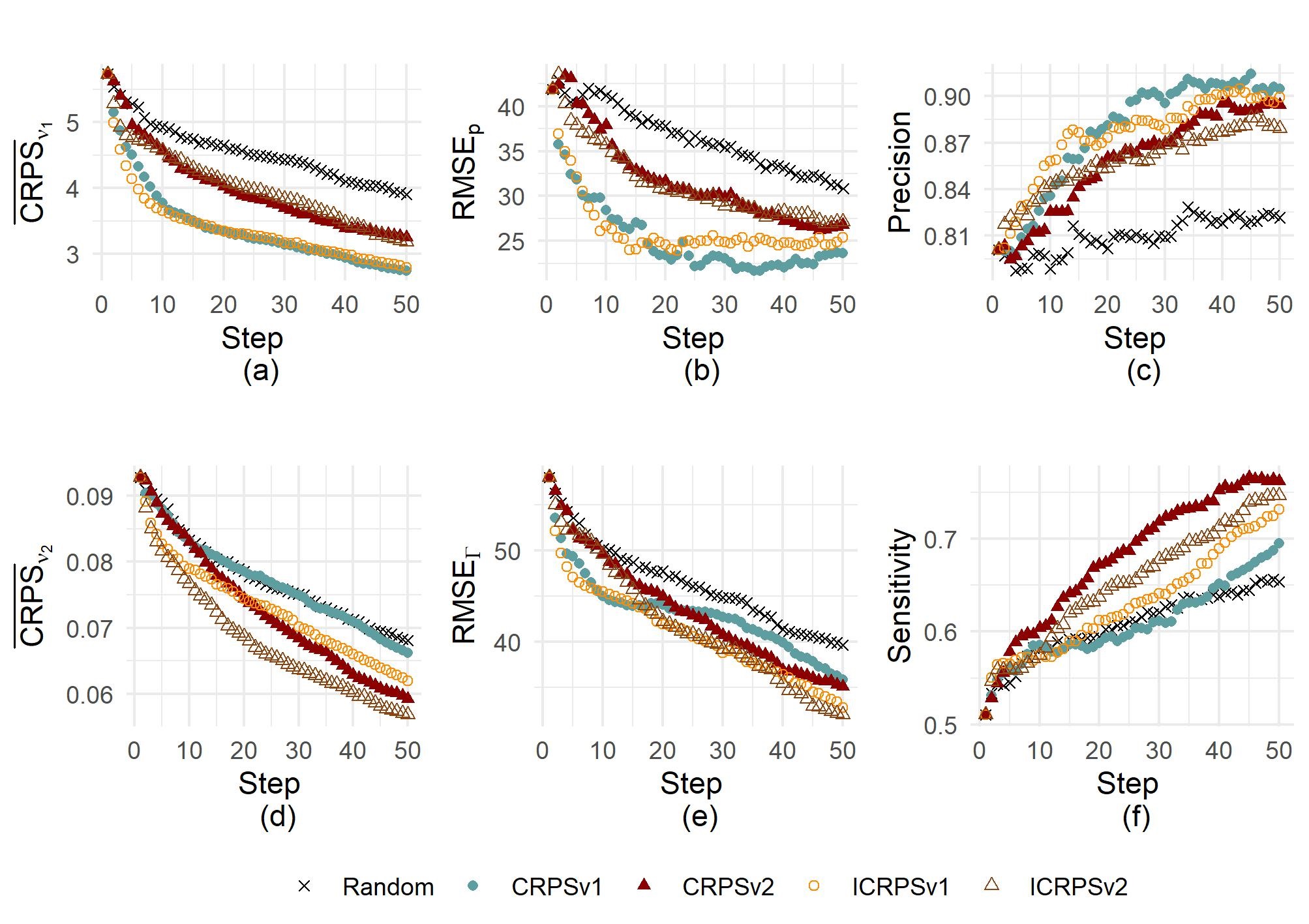
Figure 3: The sequential performance on the synthetic dataset with $M=100$ validation molecules, $n=30$ and $\widetilde{n}=50$; the mean over 60 repetitions is depicted.

To better understand the process, Figure 4 shows an example of an (a) initial model and the evolving performance for $\widetilde{n}=20$ using (b) $\mathrm{CRPS}{\nu_{1}}$ (c) and $\mathrm{CRPS}{\nu_{2}}$. The dark red dots represent the original (noisy) training set, the blue crosses indicate the predicted mean for the $M=100$ validation molecules, the light red circles indicate the added molecules, and the gray dots show the ground truth $f$. It can be clearly seen that while $\mathrm{CRPS}{\nu_{1}}$ excels in accurately predicting the responses of the TP, it is less sensitive and still has more FN compared to $\mathrm{CRPS}{\nu_{2}}$. We observe that $\mathrm{CRPS}{\nu_{1}}$ primarily adds molecules from the excursion set, while $\mathrm{CRPS}{\nu_{2}}$ focuses on molecules near the threshold, as expected based on the two weighting measures.

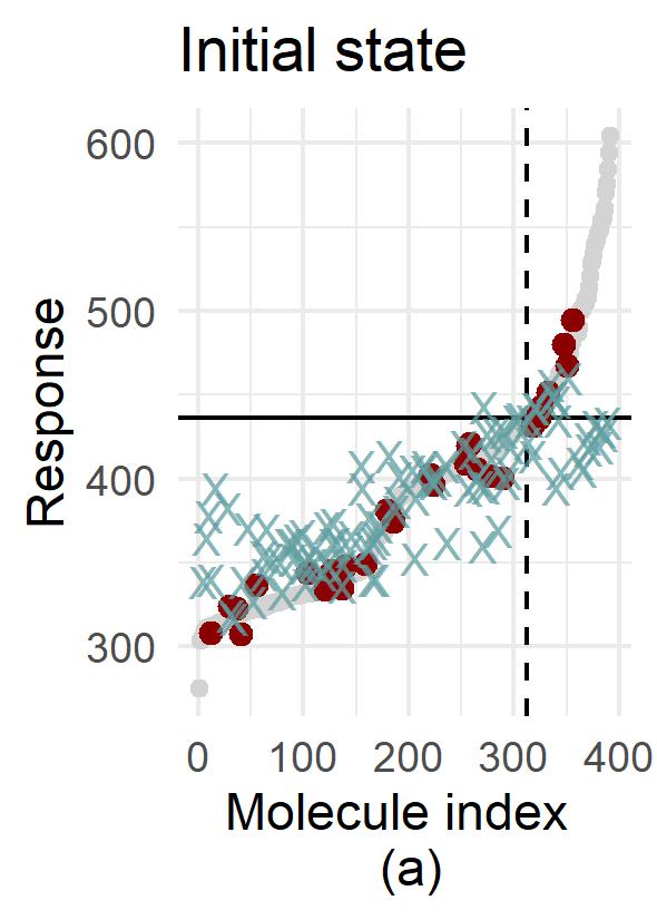
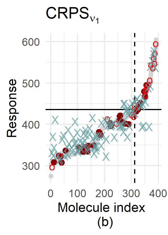
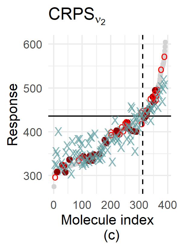
Figure 4: One illustrative example with the synthetic dataset, starting from (a) $n=30$ and adding $\widetilde{n}=20$ molecules with (b) $\mathrm{CRPS}_{\nu_{1}}$ and (c) $\mathrm{CRPS}_{\nu_{2}}$. The darkred dots show the original (noisy) training set, the blue crosses the predictive mean for the $M=100$ validation molecules, the lightred circles the added molecules and the grey dots in the back ground the ground truth $f$.

Figure 5 shows the performance of $\mathrm{CRPS}_{\nu_{2}}$ and $\mathrm{ICRPS}_{\nu_{2}}$ as a function of $\sigma_{\nu}$. For both criteria, the traditional CRPS in Figure 5(a) decreases as expected with increasing $\sigma_{\nu}$ (because then the criteria focus more and more on the whole domain, as the CRPS does). The pointwise $\mathrm{CRPS}_{\nu_{2}}$ shows a clear improvement in (b) sensitivity and a deterioration in (c) precision with increasing $\sigma_{\nu}$ (after an increase in the first point for the later). The same is also present for the SUR criterion with respect to precision, less so for sensitivity. In all previous and following results we use $\sigma_{\nu}=33$, which is half the standard deviation of the responses of the whole dataset.

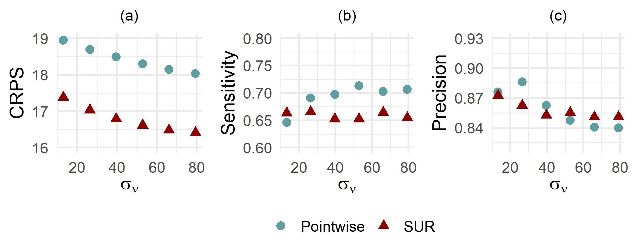
Figure 5: Performance of $\mathrm{CRPS}_{\nu_{2}}$ and $\mathrm{ICRPS}_{\nu_{2}}$ using different $\sigma_{\nu}$ for the synthetic dataset; $M=100$ validation molecules, mean over 60 repetitions, $n=30$ and $\widetilde{n}=25$.

In Figure 6, we compare the performance of the new acquisition criteria against the state-of-the-art methods. The box and whiskers plots display the distribution of the metrics obtained in 60 repetitions, highlighting the range, median and quartiles. Also in comparison with the alternative methods, the pointwise $\mathrm{CRPS}_{\nu_{1}}$ performs best with respect to the (a) $\overline{\mathrm{CRPS}}_{\nu_{1}}$ (reduction of the median compared to the random strategy by about 25 %), (b) $\mathrm{RMSE}_{p}$ (minus 40 % compared to random) and (c) precision (10 % higher than random). However, $\mathrm{ICRPS}_{\nu_{1}}$ leads to a similar performance with respect to the median in $\overline{\mathrm{CRPS}}_{\nu_{1}}$ and precision. For (d) $\overline{\mathrm{CRPS}}_{\nu_{2}}$, the performance of $\mathrm{ICRPS}_{\nu_{2}}$ is comparable to that of TIMSE, which makes sense since TIMSE also relies on a Gaussian weight around the threshold. Both reduce the median value of the random strategy by about 15 %. Regarding (e) $\mathrm{RMSE}_{\Gamma}$, the best median value is observed for TMSE (minus 20 %). The median of the (f) sensitivity is the highest for TMSE (15 % higher than for random), followed by $\mathrm{CRPS}_{\nu_{2}}$ and TIMSE.

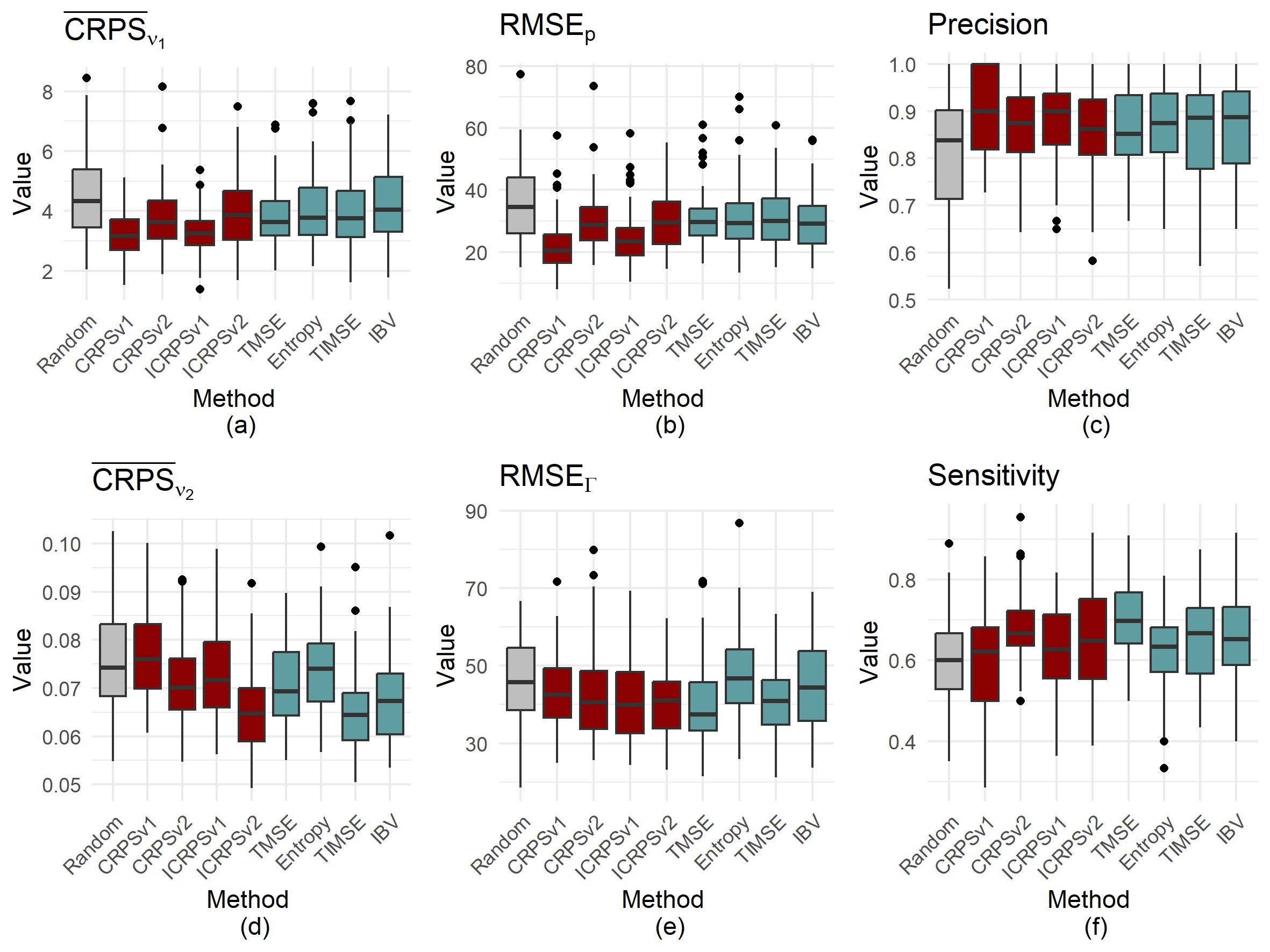
Figure 6: Performance comparison between $\mathrm{CRPS}_{\nu_{1}}$, $\mathrm{CRPS}_{\nu_{2}}$, $\mathrm{ICRPS}_{\nu_{1}}$ and $\mathrm{ICRPS}_{\nu_{2}}$ against alternative selection criteria using the synthetic dataset and $M=100$ validation molecules (60 repetitions, $n=30$ and $\widetilde{n}=25$). The box and whiskers plots depict the median, quartiles, two whiskers and all ’outlying’ points. The whiskers extend from the quartiles to the smallest / highest value at most 1.5 $\times$ the interquartile range away from the quartile, beyond which points are considered outliers.

5.2 Original dataset

For the original dataset, we only consider the box and whiskers plot for comparison (Fig. 7), with focusing solely on (a) $\overline{\mathrm{CRPS}}_{\nu_{1}}$ and (b) $\overline{\mathrm{CRPS}}_{\nu_{2}}$ (as the ground truth is not available, see Section 4.4). The pointwise $\mathrm{CRPS}_{\nu_{1}}$ also performs best for $\overline{\mathrm{CRPS}}_{\nu_{1}}$ in the original dataset and reduces the median value of the random strategy by 25 %. For $\overline{\mathrm{CRPS}}_{\nu_{2}}$, as in the synthetic case, $\mathrm{ICRPS}_{\nu_{2}}$ and TIMSE lead to similar results, with a slightly lower median for $\mathrm{ICRPS}_{\nu_{2}}$, which reduces the value of the random strategy by 15 %.

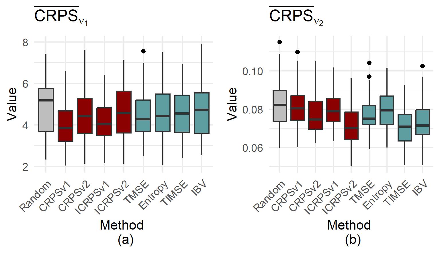
Figure 7: Comparison of the data acquisition methods using the original dataset and $M=100$ validation molecules, 60 repetitions, $n=30$ and $\widetilde{n}=25$. The box and whiskers plots depict the median, quartiles, two whiskers and all ’outlying’ points. The whiskers extend from the quartiles to the smallest / highest value at most 1.5 $\times$ the interquartile range away from the quartile, beyond which points are considered outliers.

6 Discussion and Conclusions

In this study, we use a Gaussian Process (GP) approach to model a target function, with a particular focus on an excursion set. We employ targeted sequential design strategies to efficiently select and extend the training dataset, addressing challenges in scenarios where data collection is resource intensive or costly. We introduce novel pointwise and SUR selection criteria based on the threshold-weighted CRPS, using the expected score values. The new criteria show promising performance in both a synthetic and real molecular test case, outperforming or competing with state-of-the-art methods (Fig. 6 and 7).

The test case using the synthetic version of the Photoswitch dataset highlights the following strengths and weaknesses of the new selection criteria: In terms of classification, $\mathrm{CRPS}{\nu_{1}}$ and $\mathrm{ICRPS}{\nu_{1}}$ are more precise, while $\mathrm{CRPS}{\nu_{2}}$ and $\mathrm{ICRPS}{\nu_{2}}$ are more sensitive (Fig. 3 c and f). For precision, $\mathrm{CRPS}{\nu_{1}}$ performs best, while $\mathrm{ICRPS}{\nu_{1}}$ remains precise but also outperforms the random approach in sensitivity. Regarding $\mathrm{CRPS}{\nu_{2}}$, the pointwise criterion is both more precise and sensitive. Regarding the prediction for the points identified as part of the excursion set, $\mathrm{CRPS}_{\nu_{1}}$ is highly accurate, both when considering the mean alone ($\mathrm{RMSE}_{p}$, Fig. 3b) and the predictive distribution ($\overline{\mathrm{CRPS}}_{\nu_{1}}$, Fig. 3a). But again, as for precision, $\mathrm{ICRPS}_{\nu_{1}}$ shows a similar performance and is at the same time more sensitive. Considering the points actually lying in the excursion set, $\mathrm{ICRPS}_{\nu_{2}}$ shows the strongest performance ($\overline{\mathrm{CRPS}}_{\nu_{2}}$ and $\mathrm{RMSE}_{\Gamma}$, Fig. 3d+e). Focusing on sensitivity only, $\mathrm{CRPS}{\nu_{2}}$ performs better, but $\mathrm{ICRPS}{\nu_{2}}$ does a better job when also considering the full predictive distribution.

When comparing the new criteria to state-of-the-art methods (Fig. 6), we observe that the performance of $\mathrm{CRPS}{\nu_{2}}$ and $\mathrm{ICRPS}{\nu_{2}}$ is similar to the existing TMSE and TIMSE criteria, even in terms of $\overline{\mathrm{CRPS}}_{\nu_{2}}$. This is expected, as all these methods rely on a Gaussian PDF around the threshold for targeted acquisition. On the other hand, $\mathrm{CRPS}{\nu_{1}}$ and $\mathrm{ICRPS}{\nu_{1}}$ outperform the other criteria in terms of $\overline{\mathrm{CRPS}}_{\nu_{1}}$, $\mathrm{RMSE}_{p}$, and precision (Fig. 3a-c). Entropy performed badly across all criteria, with both entropy and IBV showing notably poor performance in $\mathrm{RMSE}_{\Gamma}$ (Fig. 6e). In the real test case, where no ground truth was available (Fig. 7), we relied on $\overline{\mathrm{CRPS}}_{\nu_{1}}$ and $\overline{\mathrm{CRPS}}_{\nu_{2}}$, observing results similar to those in the synthetic test case, which helped confirm the conclusions.

There are several directions in which the presented work can be extended and deepened. Other acquisition criteria, related to expected scoring rules, can also be explored. For instance, the entropy-based criterion (Cole et al.,, 2023) is equivalent to the expected log score for a binary predictor. Similarly, the integrand of the IBV is the Bernoulli variance, which corresponds to the expectation of the Brier Score (Brier,, 1950; Murphy,, 1973). Future work could explore further alternatives to the CRPS, including multivariate scoring rules (e.g., Allen et al., 2023b, ). Within the threshold-weighted CRPS, alternative weighting measures could be explored, such as the corresponding CDF of the Gaussian $\nu_{2}$ (Allen,, 2024). This would result in a criterion that is less similar to TMSE and TIMSE. As for the criteria based on $\mathrm{CRPS}_{\nu_{1}}$, we could adjust the threshold in the weighting measure to incorporate the region around the threshold, thereby enhancing the method’s sensitivity. Next, k-step look-ahead strategies could be explored as an alternative to myopic ones. Furthermore, the initial design is currently random, what could be leveraged by employing a space-filling approach.

Declaration of Interest

The authors report there are no competing interests to declare.

Appendix A Appendix

A.1 More on Gaussian Process modeling

Here, we expand on Section 2.1 and provide additional details on the distribution of a GP $\boldsymbol{\xi}$ conditioned on $\mathcal{A}_{n}$, denoted by $\boldsymbol{\xi_{n}}=\left(\xi_{n}(\boldsymbol{x})\right)_{\boldsymbol{x}\in\mathcal{X}}$. Under mild conditions (invertibility of the matrix $\boldsymbol{K_{\mathrm{obs}}}$), $\boldsymbol{\xi_{n}}$ remains a GP. Indeed, if the mean $m$ of the prior GP $\boldsymbol{\xi}$ is assumed to be known and constant, this refers to the setting of simple kriging (Chiles and Delfiner,, 2012). In practice, the mean function may be unknown, which motivates so-called ordinary kriging with a constant unknown mean and universal kriging, where the mean is assumed to be a linear combination of prescribed basis functions with unknown coefficients. In this work, we focus on the case of ordinary kriging, where $\boldsymbol{\xi_{n}}\sim\mathrm{GP}\left(m_{n},k_{n}\right)$ with the conditional mean function $m_{n}:\mathcal{X}\to\mathbb{R}$ and conditional covariance function $k_{n}:\mathcal{X}\times\mathcal{X}\to\mathbb{R}$ being defined as (for $\boldsymbol{x},\boldsymbol{x^{\prime}}\in\mathcal{X}$):

$$m_{n}(\boldsymbol{x})=\hat{\beta}+\boldsymbol{K}^{\top}_{\mathrm{cross}}(\boldsymbol{x})\boldsymbol{K}_{\mathrm{obs}}^{-1}(\boldsymbol{z_{n}}-\hat{\beta}\mathbf{1}_{n}),$$ (19)

$$k_{n}(\boldsymbol{x},\boldsymbol{x^{\prime}})=k(\boldsymbol{x},\boldsymbol{x^{\prime}})-\boldsymbol{K}^{\top}_{\mathrm{cross}}(\boldsymbol{x})\boldsymbol{K}_{\mathrm{obs}}^{-1}\boldsymbol{K}_{\mathrm{cross}}(\boldsymbol{x^{\prime}})$$

$$\hskip 52.0pt+\frac{\left(1-\boldsymbol{K}^{\top}_{\mathrm{cross}}(\boldsymbol{x})\boldsymbol{K}_{\mathrm{obs}}^{-1}\mathbf{1}_{n}\right)^{\top}\left(1-\boldsymbol{K}^{\top}_{\mathrm{cross}}(\boldsymbol{x^{\prime}})\boldsymbol{K}_{\mathrm{obs}}^{-1}\mathbf{1}_{n}\right)}{\mathbf{1}^{\top}_{n}\boldsymbol{K}_{\mathrm{obs}}^{-1}\mathbf{1}_{n}},$$

with $\mathbf{1}_{n}$ denoting the vector of $1$s of size $n$, $\boldsymbol{K}_{\mathrm{cross}}(\boldsymbol{x})=[k(\boldsymbol{x},\boldsymbol{x_{i}})]_{1\leq i\leq n}$ and the estimator of the mean $\hat{\beta}=\frac{\mathbf{1}^{\top}_{n}\boldsymbol{K}_{\mathrm{obs}}^{-1}\boldsymbol{z_{n}}}{\mathbf{1}^{\top}_{n}\boldsymbol{K}_{\mathrm{obs}}^{-1}\mathbf{1}_{n}}$.

In the context of sequential data acquisition, we can facilitate the computations by considering updating formulas (Emery,, 2009; Chevalier et al., 2013b, ). Considering the expanded observation event $\mathcal{A}_{n+1}=\{\boldsymbol{Z_{n}}=\boldsymbol{z_{n}},Z_{n+1}=z_{n+1}\}$ with $z_{n+1}=f(\boldsymbol{x_{n+1}})+\epsilon_{n+1}$, the mean and covariance function of $\boldsymbol{\xi_{n+1}}\sim\mathrm{GP}(m_{n+1},k_{n+1})$ can be updated as:

$$m_{n+1}(\boldsymbol{x})=m_{n}(\boldsymbol{x})+\frac{k_{n}(\boldsymbol{x_{n+1}},\boldsymbol{x})}{(k_{n}(\boldsymbol{x_{n+1}},\boldsymbol{x_{n+1}})+\tau^{2})}\left(z_{n+1}-m_{n}(\boldsymbol{x_{n+1}})\right),$$ (20)

$$k_{n+1}(\boldsymbol{x},\boldsymbol{x^{\prime}})=k_{n}(\boldsymbol{x},\boldsymbol{x^{\prime}})-\frac{k_{n}(\boldsymbol{x_{n+1}},\boldsymbol{x})k_{n}(\boldsymbol{x_{n+1}},\boldsymbol{x^{\prime}})}{(k_{n}(\boldsymbol{x_{n+1}},\boldsymbol{x_{n+1}})+\tau^{2})}.$$

A.2 Kernel comparison with the (original) Photoswitch dataset

Classically used families of covariance kernels for Euclidean input spaces include notably the family of isotropic Matérn kernels, encompassing the isotropic exponential and Gaussian (or square-exponential) covariance kernels as limiting cases (Stein,, 2012). Isotropy means in this context that kernel values between pairs of locations depend on the Euclidean distance between them. In multidimensional settings, anisotropic extensions of such kernels are also commonplace. The isotropic exponential and Gaussian kernels are given by,

$$k_{\mathrm{EXP}}(\boldsymbol{x},\boldsymbol{x^{\prime}})=\sigma_{k}^{2}\exp\left(-\frac{||\boldsymbol{x}-\boldsymbol{x^{\prime}}||}{\theta_{k}}\right),\quad k_{\mathrm{GAU}}(\boldsymbol{x},\boldsymbol{x^{\prime}})=\sigma_{k}^{2}\exp\left(-\frac{||\boldsymbol{x}-\boldsymbol{x^{\prime}}||^{2}}{2\theta_{k}^{2}}\right),$$ (21)

using the Euclidean distance between the input locations, $||\boldsymbol{x}-\boldsymbol{x^{\prime}}||=\sqrt{(\boldsymbol{x}-\boldsymbol{x^{\prime}})^{\top}(\boldsymbol{x}-\boldsymbol{x^{\prime}})}$ and the variance parameter $\sigma_{k}^{2}>0$ and correlation length $\theta_{k}>0$.

For the choice of kernel used on the original dataset, we compare the performance of the Tanimoto, Gaussian and Exponential kernels using $10,20,30\%$ of the points for training, as shown in Table 1. The Tanimoto kernel consistently outperforms the Exponential kernel in all scenarios for RMSE and CRPS. Interestingly, while the Gaussian kernel showed comparable performance to the Tanimoto kernel when trained on 20 or 30 $\%$ of the data, it performed exceptionally poorly with only 10$\%$. This may be due to difficulties in estimating the hyperparameters of the kernel with only $n=39$ molecules. Given the consistent performance of the Tanimoto kernel, even with small training datasets, we use it for our sequential work on molecules, especially as it is more interpretable than a stationary kernel in this context.

Kernel	$k_{\mathrm{TAN}}$	$k_{\mathrm{EXP}}$	$k_{\mathrm{GAU}}$	$k_{\mathrm{TAN}}$	$k_{\mathrm{EXP}}$	$k_{\mathrm{GAU}}$	$k_{\mathrm{TAN}}$	$k_{\mathrm{EXP}}$	$k_{\mathrm{GAU}}$
$n$	$10\%$			$20\%$			$30\%$
RMSE	40.07	41.37	55.65	33.32	34.62	35.44	29.70	30.94	29.90
CRPS	21.65	22.60	31.52	17.78	18.87	18.96	15.74	16.83	15.62

Table 1: RMSE and CRPS values for different train/test splits using the Tanimoto, exponential, and Gaussian kernels (averaged over the same 30 random splits for each).

A.3 Proofs threshold-weighted CRPS

A.3.1 Theorem 1: Scoring Rules

It holds that,

$$\mathrm{CRPS}_{\nu_{1}}(\Phi_{\mu,\sigma^{2}},y)=\int_{-\infty}^{\infty}\left[\Phi\left(\frac{u-\mu}{\sigma}\right)-\mathbbm{1}\{y\leq u\}\right]^{2}\mathbbm{1}\{t\leq u\}\,\mathrm{d}u=\mathrm{CRPS}(\Phi_{\mu,\sigma^{2}}^{t},y^{t}),$$

with the traditional CRPS for the left-censored Gaussian $\Phi_{\mu,\sigma^{2}}^{t}(u)=\Phi\left(\frac{u-\mu}{\sigma}\right)\mathbbm{1}\{u\geq t\}$ and censored value $y^{t}=\max(y,t)$ (Allen et al., 2023a, ):

$$\mathrm{CRPS}(\Phi_{\mu,\sigma^{2}}^{t},y^{t}) =\int_{-\infty}^{\infty}\left[\Phi\left(\frac{u-\mu}{\sigma}\right)\mathbbm{1}\{t\leq u\}-\mathbbm{1}\{\max(y,t)\leq u\}\right]^{2}\,\mathrm{d}u$$

$$=\int_{-\infty}^{t}\mathbbm{1}\{\max(y,t)\leq u\}\,\mathrm{d}u+\int_{t}^{\infty}\left[\Phi\left(\frac{u-\mu}{\sigma}\right)-\mathbbm{1}\{\max(y,t)\leq u\}\right]^{2}\,\mathrm{d}u$$

$$=\int_{\infty}^{\infty}\left[\Phi\left(\frac{u-\mu}{\sigma}\right)-\mathbbm{1}\{\max(y,t)\leq u\}\right]^{2}\mathbbm{1}\{u\geq t\}\,\mathrm{d}u$$

$$=\int_{\infty}^{\infty}\left[\Phi\left(\frac{u-\mu}{\sigma}\right)-\mathbbm{1}\{y\leq u\}\mathbbm{1}\{t\leq u\}\right]^{2}\mathbbm{1}\{u\geq t\}\,\mathrm{d}u$$

$$=\int_{-\infty}^{\infty}\left[\Phi\left(\frac{u-\mu}{\sigma}\right)-\mathbbm{1}\{y\leq u\}\right]^{2}\mathbbm{1}\{u\geq t\}\,\mathrm{d}u.$$

The CRPS for a censored normal distribution has an analytical formula (Jordan et al.,, 2019). For a left-censored standard normal distribution $\Phi^{t}$ with upper bound $\infty$, lower bound $t$ and a point mass of $L$ at the lower bound, it holds,

$$\mathrm{CRPS}(\Phi^{t},y^{t}) =-tL^{2}+\frac{(1-L)}{\left(1-\Phi(t)\right)}y^{t}\left(2\Phi(y^{t})-\frac{(1-2L)+\Phi(t)}{1-L}\right)$$

$$\quad\quad+\frac{(1-L)}{\left(1-\Phi(t)\right)}\left(2\phi\left(y^{t}\right)-2\phi\left(t\right)L\right)$$

$$\quad\quad-\left(\frac{(1-L)}{\left(1-\Phi(t)\right)}\right)^{2}\frac{1}{\sqrt{\pi}}\left(1-\Phi(t\sqrt{2})\right).$$

By using the transformation formula for a censored normal distribution $\Phi_{\mu,\sigma^{2}}^{t}$ (Jordan et al.,, 2019) and the point mass in $t$ being $L=\Phi_{\mu,\sigma^{2}}(t)=\Phi(\widetilde{t})$ for $\widetilde{t}=(t-\mu)/\sigma$, we denote by $\widetilde{y^{t}}=\Big{(}\max(y,t)-\mu\Big{)}/\sigma$ and get,

$$\mathrm{CRPS}_{\nu_{1}}(\Phi_{\mu,\sigma^{2}},y) =\mathrm{CRPS}(\Phi_{\mu,\sigma^{2}}^{t},y^{t})=\sigma\;\mathrm{CRPS}\left(\Phi^{\widetilde{t}},\widetilde{y^{t}}\right)$$

$$=\sigma\left[-\widetilde{t}\Phi(\widetilde{t})^{2}+\frac{\left(1-\Phi(\widetilde{t})\right)}{\left(1-\Phi(\widetilde{t})\right)}\widetilde{y^{t}}\left(2\Phi(\widetilde{y^{t}})-\frac{\left(1-2\Phi(\widetilde{t})\right)+\Phi(\widetilde{t})}{1-\Phi(\widetilde{t})}\right)\right.$$

$$\quad\quad+\frac{\left(1-\Phi(\widetilde{t})\right)}{\left(1-\Phi(\widetilde{t})\right)}\left(2\phi\left(\widetilde{y^{t}}\right)-2\phi\left(\widetilde{t}\right)\Phi(\widetilde{t})\right)\left.-\left(\frac{\left(1-\Phi(\widetilde{t})\right)}{\left(1-\Phi(\widetilde{t})\right)}\right)^{2}\frac{1}{\sqrt{\pi}}\left(1-\Phi(\widetilde{t}\sqrt{2})\right)\right]$$

$$=\sigma\left[-\widetilde{t}\Phi(\widetilde{t})^{2}+\widetilde{y^{t}}\left(2\Phi(\widetilde{y^{t}})-1\right)+\left(2\phi\left(\widetilde{y^{t}}\right)-2\phi\left(\widetilde{t}\right)\Phi(\widetilde{t})\right)-\frac{1}{\sqrt{\pi}}\left(1-\Phi(\widetilde{t}\sqrt{2})\right)\right].$$

For $\nu_{2}$, we derive:

$$\mathrm{CRPS}_{\nu_{2}}(\Phi_{\mu,\sigma^{2}},y) =\int_{-\infty}^{\infty}\left[\Phi\left(\frac{u-\mu}{\sigma}\right)-\mathbbm{1}\{y\leq u\}\right]^{2}\phi\left(\frac{u-t}{\sigma_{\nu}}\right)\frac{1}{\sigma_{\nu}}\,\mathrm{d}u$$

$$=\underbrace{\int_{-\infty}^{\infty}\Phi\left(\frac{u-\mu}{\sigma}\right)^{2}\phi\left(\frac{u-t}{\sigma_{\nu}}\right)\frac{1}{\sigma_{\nu}}\,\mathrm{d}u}_{(1)}$$

$$\quad\quad-2\underbrace{\int_{-\infty}^{\infty}\Phi\left(\frac{u-\mu}{\sigma}\right)\mathbbm{1}\{y\leq u\}\phi\left(\frac{u-t}{\sigma_{\nu}}\right)\frac{1}{\sigma_{\nu}}\,\mathrm{d}u}_{(2)}$$

$$\quad\quad+\underbrace{\int_{-\infty}^{\infty}\mathbbm{1}\{y\leq u\}\phi\left(\frac{u-t}{\sigma_{\nu}}\right)\frac{1}{\sigma_{\nu}}\,\mathrm{d}u}_{(3)}.$$

The three parts can be simplified as follows:
(1) For $N,\widetilde{N},U^{\prime}\overset{i.i.d.}{\sim}\mathcal{N}(0,1)$ and using a variable transform $u^{\prime}=\frac{u-t}{\sigma_{\nu}}$:

$$\int_{-\infty}^{\infty}\Phi\left(\frac{u-\mu}{\sigma}\right)^{2}\frac{1}{\sigma_{\nu}}\phi\left(\frac{u-t}{\sigma_{\nu}}\right)\,\mathrm{d}u =\int_{-\infty}^{\infty}\Phi\left(\frac{\sigma_{\nu}u^{\prime}+t-\mu}{\sigma}\right)^{2}\phi\left(u^{\prime}\right)\,\mathrm{d}u^{\prime}$$

$$=\int_{-\infty}^{\infty}\mathbb{P}\left(N\leq\frac{\sigma_{\nu}u^{\prime}+t-\mu}{\sigma}\right)\mathbb{P}\left(\widetilde{N}\leq\frac{\sigma_{\nu}u^{\prime}+t-\mu}{\sigma}\right)\phi\left(u^{\prime}\right)\,\mathrm{d}u^{\prime}$$

$$=\mathbb{P}\left(\sigma N-t+\mu-\sigma_{\nu}U^{\prime}\leq 0,\sigma\widetilde{N}-t+\mu-\sigma_{\nu}U^{\prime}\leq 0\right)$$

$$=\Phi\left(\begin{pmatrix}0\\ 0\end{pmatrix};\begin{pmatrix}\mu-t\\ \mu-t\end{pmatrix},\begin{pmatrix}\sigma_{\nu}^{2}+\sigma^{2}&\sigma_{\nu}^{2}\\ \sigma_{\nu}^{2}&\sigma_{\nu}^{2}+\sigma^{2}\end{pmatrix}\right)$$

(2) For $V,U^{\prime}\overset{i.i.d.}{\sim}\mathcal{N}(0,1)$ and using again $u^{\prime}=\frac{u-t}{\sigma_{\nu}}$:

$$\int_{-\infty}^{\infty} \Phi\left(\frac{u-\mu}{\sigma}\right)\mathbbm{1}\{y\leq u\}\phi\left(\frac{u-t}{\sigma_{\nu}}\right)\frac{1}{\sigma_{\nu}}\,\mathrm{d}u$$

$$=\int_{-\infty}^{\infty}\Phi\left(\frac{\sigma_{\nu}u^{\prime}+t-\mu}{\sigma}\right)\mathbbm{1}\{y\leq\sigma_{\nu}u^{\prime}+t\}\;\phi\left(u^{\prime}\right)\,\mathrm{d}u^{\prime}$$

$$=\int_{-\infty}^{\infty}\int_{-\infty}^{\infty}\mathbbm{1}\{v\leq\frac{\sigma_{\nu}u^{\prime}+t-\mu}{\sigma}\}\,\phi(v)\,\mathrm{d}v\,\mathbbm{1}\{y\leq\sigma_{\nu}u^{\prime}+t\}\;\phi\left(u^{\prime}\right)\,\mathrm{d}u^{\prime}$$

$$=\mathbb{P}\left(\sigma V-\sigma_{\nu}U^{\prime}+\mu-t\leq 0,y-\sigma_{\nu}U^{\prime}-t\leq 0\right)$$

$$=\Phi\left(\begin{pmatrix}0\\ 0\end{pmatrix};\begin{pmatrix}\mu-t\\ y-t\end{pmatrix},\begin{pmatrix}\sigma_{\nu}^{2}+\sigma^{2}&\sigma_{\nu}^{2}\\ \sigma_{\nu}^{2}&\sigma_{\nu}^{2}\end{pmatrix}\right)$$

(3) Reusing $u^{\prime}=\frac{u-t}{\sigma_{\nu}}$, it holds that:

$$\int_{-\infty}^{\infty}\mathbbm{1}\{y\leq u\}\phi\left(\frac{u-t}{\sigma_{\nu}}\right)\frac{1}{\sigma_{\nu}}\,\mathrm{d}u=\int_{-\infty}^{\infty}\mathbbm{1}\{\frac{y-t}{\sigma_{\nu}}\leq u^{\prime}\}\phi\left(u^{\prime}\right)\mathrm{d}u^{\prime}=\Phi\left(\frac{t-y}{\sigma_{\nu}}\right)$$

Eventually, we obtain:

$$\mathrm{CRPS}_{\nu_{2}}(\Phi_{\mu,\sigma^{2}},y) =\Phi\left(\begin{pmatrix}0\\ 0\end{pmatrix};\begin{pmatrix}\mu-t\\ \mu-t\end{pmatrix},\begin{pmatrix}\sigma_{\nu}^{2}+\sigma^{2}&\sigma_{\nu}^{2}\\ \sigma_{\nu}^{2}&\sigma_{\nu}^{2}+\sigma^{2}\end{pmatrix}\right)$$

$$\quad\quad-2\Phi\left(\begin{pmatrix}0\\ 0\end{pmatrix};\begin{pmatrix}\mu-t\\ y-t\end{pmatrix},\begin{pmatrix}\sigma_{\nu}^{2}+\sigma^{2}&\sigma_{\nu}^{2}\\ \sigma_{\nu}^{2}&\sigma_{\nu}^{2}\end{pmatrix}\right)+\Phi\left(\frac{t-y}{\sigma_{\nu}}\right).$$

A.3.2 Theorem 2: Pointwise criteria

Let us start with the general result, where $\rho(\cdot)$ denotes the PDF $F$:

$$\mathrm{CRPS}_{\nu}(F) =\int_{-\infty}^{\infty}\mathrm{CRPS}_{\nu}(F,y^{\prime})\rho(y^{\prime})\,\mathrm{d}y^{\prime}$$

$$=\int_{-\infty}^{\infty}\int_{-\infty}^{\infty}[F(u)-\mathbbm{1}\{y^{\prime}\leq u\}]^{2}\,\mathrm{d}\nu(u)\,\rho(y^{\prime})\,\mathrm{d}y^{\prime}$$

$$=\int_{-\infty}^{\infty}\int_{-\infty}^{\infty}\left[F(u)^{2}-2F(u)\mathbbm{1}\{y^{\prime}\leq u\}+\mathbbm{1}\{y^{\prime}\leq u\}\right]\,\rho(y^{\prime})\,\mathrm{d}y^{\prime}\,\mathrm{d}\nu(u)$$

$$=\int_{-\infty}^{\infty}\left[F(u)^{2}-2F(u)^{2}+F(u)\right]\,\mathrm{d}\nu(u)$$

$$=\int F(u)\left(1-F(u)\right)\,\mathrm{d}\nu(u)$$

Let us consider $F=\Phi_{\mu,\sigma^{2}}$ and the first representation for $\nu_{1}$. With defining $u^{\left(\widetilde{t}\right)}=\max(u,\widetilde{t})$ and transforming $u=\frac{y^{\prime}-\mu}{\sigma}$, we get:

$$\mathrm{CRPS}_{\nu_{1}}(\Phi_{\mu,\sigma^{2}}) =\int\mathrm{CRPS}_{\nu_{1}}(\Phi_{\mu,\sigma^{2}},y^{\prime})\phi_{\mu,\sigma^{2}}(y^{\prime})\mathrm{d}y^{\prime}$$

$$=\int\mathrm{CRPS}(\Phi_{\mu,\sigma^{2}}^{t},\max(y^{\prime},t))\phi\left(\frac{y^{\prime}-\mu}{\sigma}\right)\frac{1}{\sigma}\mathrm{d}y^{\prime}$$

$$=\int\mathrm{CRPS}(\Phi_{\mu,\sigma^{2}}^{t},\max(\sigma u+\mu,t))\phi(u)\mathrm{d}u$$

$$=\int\sigma\mathrm{CRPS}\left(\Phi^{\widetilde{t}},u^{\left(\widetilde{t}\right)}\right)\phi(u)\mathrm{d}u$$

$$=\int\sigma\Big{[}-\widetilde{t}\Phi(\widetilde{t})^{2}+u^{\left(\widetilde{t}\right)}\left(2\Phi\left(u^{\left(\widetilde{t}\right)}\right)-1\right)+\left(2\phi\left(u^{\left(\widetilde{t}\right)}\right)-2\phi\left(\widetilde{t}\right)\Phi(\widetilde{t})\right)$$

$$\quad\quad-\frac{1}{\sqrt{\pi}}\left(1-\Phi(\widetilde{t}\sqrt{2})\right)\Big{]}\phi(u)\mathrm{d}u$$

$$=\sigma\underbrace{\int-\widetilde{t}\Phi(\widetilde{t})^{2}\phi(u)\mathrm{d}u}_{=-\widetilde{t}\Phi(\widetilde{t})^{2}}+\sigma\underbrace{\int u^{\left(\widetilde{t}\right)}\left(2\Phi(u^{\left(\widetilde{t}\right)})-1\right)\phi(u)\mathrm{d}u}_{(1)}$$

$$\quad\quad+\sigma\underbrace{\int\left(2\phi\left(u^{\left(\widetilde{t}\right)}\right)-2\phi\left(\widetilde{t}\right)\Phi(\widetilde{t})\right)\phi(u)\mathrm{d}u}_{(2)}-\sigma\underbrace{\int\frac{1}{\sqrt{\pi}}\left(1-\Phi(\widetilde{t}\sqrt{2})\right)\phi(u)\mathrm{d}u}_{=\frac{1}{\sqrt{\pi}}\left(1-\Phi(\widetilde{t}\sqrt{2})\right)}.$$

The details for the two numbered parts are as follows:
(1) Using Owen, (1980) Equations (1011.1) and (11):

$$\int u^{\left(\widetilde{t}\right)} \left(2\Phi\left(u^{\left(\widetilde{t}\right)}\right)-1\right)\phi(u)\mathrm{d}u=\int_{-\infty}^{\widetilde{t}}\widetilde{t}\left(2\Phi(\widetilde{t})-1\right)\phi(u)\mathrm{d}u+\int_{\widetilde{t}}^{\infty}u\left(2\Phi(u)-1\right)\phi(u)\mathrm{d}u$$

$$=\widetilde{t}\left(2\Phi(\widetilde{t})-1\right)\Phi(\widetilde{t})+2\int_{\widetilde{t}}^{\infty}u\Phi(u)\phi(u)\mathrm{d}u-\int_{\widetilde{t}}^{\infty}u\phi(u)\mathrm{d}$$

$$=\widetilde{t}\left(2\Phi(\widetilde{t})-1\right)\Phi(\widetilde{t})+2\Big{[}\frac{1}{2\sqrt{\pi}}\Phi(u\sqrt{2})-\phi(u)\Phi(u)\Big{]}_{\widetilde{t}}^{\infty}-\Big{[}-\phi(u)\Big{]}_{\widetilde{t}}^{\infty}$$

$$=\widetilde{t}\left(2\Phi(\widetilde{t})-1\right)\Phi(\widetilde{t})+\frac{1}{\sqrt{\pi}}-\frac{1}{\sqrt{\pi}}\Phi(\widetilde{t}\sqrt{2})+2\phi(\widetilde{t})\Phi(\widetilde{t})-\phi(\widetilde{t})$$

$$=2\widetilde{t}\Phi(\widetilde{t})^{2}-\widetilde{t}\Phi(\widetilde{t})+\frac{1}{\sqrt{\pi}}-\frac{1}{\sqrt{\pi}}\Phi(\widetilde{t}\sqrt{2})+2\phi(\widetilde{t})\Phi(\widetilde{t})-\phi(\widetilde{t})$$

(2) Using Owen, (1980) Equation (20)

$$\int \left(2\phi\left(u^{\left(\widetilde{t}\right)}\right)-2\phi\left(\widetilde{t}\right)\Phi(\widetilde{t})\right)\phi(u)\mathrm{d}u$$

$$=\int_{-\infty}^{\widetilde{t}}\left(2\phi\left(\widetilde{t}\right)-2\phi\left(\widetilde{t}\right)\Phi(\widetilde{t})\right)\phi(u)\mathrm{d}u+\int_{\widetilde{t}}^{\infty}\left(2\phi\left(u\right)-2\phi\left(\widetilde{t}\right)\Phi(\widetilde{t})\right)\phi(u)\mathrm{d}u$$

$$=\left(2\phi\left(\widetilde{t}\right)-2\phi\left(\widetilde{t}\right)\Phi(\widetilde{t})\right)\Phi(\widetilde{t})+2\int_{\widetilde{t}}^{\infty}\phi\left(u\right)^{2}\mathrm{d}u-2\phi\left(\widetilde{t}\right)\Phi(\widetilde{t})\int_{\widetilde{t}}^{\infty}\phi(u)\mathrm{d}u$$

$$=\left(2\phi\left(\widetilde{t}\right)-2\phi\left(\widetilde{t}\right)\Phi(\widetilde{t})\right)\Phi(\widetilde{t})+2\Big{[}\frac{1}{2\sqrt{\pi}}\Phi(u\sqrt{2})\Big{]}_{\widetilde{t}}^{\infty}-2\phi\left(\widetilde{t}\right)\Phi(\widetilde{t})(1-\Phi(\widetilde{t}))$$

$$=\left(2\phi\left(\widetilde{t}\right)-2\phi\left(\widetilde{t}\right)\Phi(\widetilde{t})\right)\Phi(\widetilde{t})+\frac{1}{\sqrt{\pi}}\left(1-\Phi(\widetilde{t}\sqrt{2})\right)-2\phi\left(\widetilde{t}\right)\Phi(\widetilde{t})(1-\Phi(\widetilde{t}))$$

$$=2\phi\left(\widetilde{t}\right)\Phi(\widetilde{t})-2\phi\left(\widetilde{t}\right)\Phi(\widetilde{t})^{2}+\frac{1}{\sqrt{\pi}}\left(1-\Phi(\widetilde{t}\sqrt{2})\right)-2\phi\left(\widetilde{t}\right)\Phi(\widetilde{t})+2\phi\left(\widetilde{t}\right)\Phi(\widetilde{t})^{2}$$

$$=\frac{1}{\sqrt{\pi}}\left(1-\Phi(\widetilde{t}\sqrt{2})\right)$$

Eventually, we get:

$$\mathrm{CRPS}_{\nu_{1}}(\Phi_{\mu,\sigma^{2}}) =\sigma\Big{[}-\widetilde{t}\Phi(\widetilde{t})^{2}+2\widetilde{t}\Phi(\widetilde{t})^{2}-\widetilde{t}\Phi(\widetilde{t})+\frac{1}{\sqrt{\pi}}-\frac{1}{\sqrt{\pi}}\Phi(\widetilde{t}\sqrt{2})+2\phi(\widetilde{t})\Phi(\widetilde{t})-\phi(\widetilde{t})$$

$$\quad\quad+\frac{1}{\sqrt{\pi}}\left(1-\Phi(\widetilde{t}\sqrt{2})\right)-\frac{1}{\sqrt{\pi}}\left(1-\Phi(\widetilde{t}\sqrt{2})\right)\Big{]}$$

$$=\sigma\Big{[}\widetilde{t}\Phi(\widetilde{t})^{2}-\widetilde{t}\Phi(\widetilde{t})+\frac{1}{\sqrt{\pi}}-\frac{1}{\sqrt{\pi}}\Phi(\widetilde{t}\sqrt{2})+2\phi(\widetilde{t})\Phi(\widetilde{t})-\phi(\widetilde{t})\Big{]}$$

The alternative representation is obtained using $N,\widetilde{N}\overset{i.i.d.}{\sim}\mathcal{N}(0,1)$ and $u^{\prime}=\frac{u-\mu}{\sigma}$:

$$\mathrm{CRPS}_{\nu_{1}}(\Phi_{\mu,\sigma^{2}}) =\int_{t}^{\infty}\Phi\left(\frac{u-\mu}{\sigma}\right)\left(1-\Phi\left(\frac{u-\mu}{\sigma}\right)\right)\,\mathrm{d}u$$

$$=\int_{t}^{\infty}\mathbb{P}\left(N\leq\frac{u-\mu}{\sigma}\right)\mathbb{P}\left(\widetilde{N}\geq\frac{u-\mu}{\sigma}\right)\,\mathrm{d}u$$

$$=\int_{t}^{\infty}\mathbb{E}\left[\mathbbm{1}\left(N\leq\frac{u-\mu}{\sigma}\leq\widetilde{N}\right)\right]\,\mathrm{d}u$$

$$=\mathbb{E}\left[\int\mathbbm{1}\left(\max\left(N,\frac{t-\mu}{\sigma}\right)\leq\frac{u-\mu}{\sigma}\leq\widetilde{N}\right)\,\mathrm{d}u\right]$$

$$=\mathbb{E}\left[\sigma\int\mathbbm{1}\left(\max\left(N,\frac{t-\mu}{\sigma}\right)\leq u^{\prime}\leq\widetilde{N}\right)\,\mathrm{d}u^{\prime}\right]$$

$$=\sigma\mathbb{E}\left[\left(\widetilde{N}-\max\left(N,\frac{t-\mu}{\sigma}\right)\right)_{+}\right].$$

For $\nu_{2}$, assuming $N,\widetilde{N},N^{\prime}\sim\mathcal{N}(0,1)$ independent and transform $n^{\prime}=\frac{u-t}{\sigma_{\nu}}$, we get:

$$\mathrm{CRPS}_{\nu_{2}}(\Phi_{\mu,\sigma^{2}}) =\int\Phi\left(\frac{u-\mu}{\sigma}\right)\left(1-\Phi\left(\frac{u-\mu}{\sigma}\right)\right)\frac{1}{\sigma_{\nu}}\phi\left(\frac{u-t}{\sigma_{\nu}}\right)\,\mathrm{d}u$$

$$=\int\mathbb{P}\left(N\leq\frac{u-\mu}{\sigma}\right)\mathbb{P}\left(\widetilde{N}\leq-\frac{u-\mu}{\sigma}\right)\frac{1}{\sigma_{\nu}}\phi\left(\frac{u-t}{\sigma_{\nu}}\right)\,\mathrm{d}u$$

$$=\int\mathbb{P}\left(N\leq\frac{t+\sigma_{\nu}n^{\prime}-\mu}{\sigma}\right)\mathbb{P}\left(\widetilde{N}\leq-\frac{t+\sigma_{\nu}n^{\prime}-\mu}{\sigma}\right)\phi\left(n^{\prime}\right)\,\mathrm{d}n^{\prime}$$

$$=\mathbb{P}\left(N^{\prime}\geq\frac{\sigma N-t+\mu}{\sigma_{\nu}},N^{\prime}\leq\frac{-\sigma\widetilde{N}-t+\mu}{\sigma_{\nu}}\right)$$

$$=\mathbb{P}\left(\sigma N-t+\mu-\sigma_{\nu}N^{\prime}\leq 0,\sigma\widetilde{N}+t-\mu+\sigma_{\nu}N^{\prime}\leq 0\right)$$

$$=\Phi\left(\begin{pmatrix}0\\ 0\end{pmatrix};\begin{pmatrix}\mu-t\\ t-\mu\end{pmatrix},\begin{pmatrix}\sigma_{\nu}^{2}+\sigma^{2}&-\sigma_{\nu}^{2}\\ -\sigma_{\nu}^{2}&\sigma_{\nu}^{2}+\sigma^{2}\end{pmatrix}\right)$$

A.3.3 Theorem 3: SUR criteria

Recall that we consider the conditional GP $\boldsymbol{\xi}_{n+1}\sim\mathrm{GP}(m_{n+1},k_{n+1})$ and its predecessor $\boldsymbol{\xi_{n}}\sim\mathrm{GP}(m_{n},k_{n})$. For fixed $\boldsymbol{x^{\prime}}\in\mathcal{X}$ and using $\sigma^{2}_{n+1}=k_{n+1}(\boldsymbol{x^{\prime}},\boldsymbol{x^{\prime}})$, $\mu_{n}=m_{n}(\boldsymbol{x^{\prime}})$, $\alpha_{n}=\alpha_{n}(\boldsymbol{x^{\prime}})$, we start with some general reformulations ($N,\widetilde{N},V\overset{i.i.d.}{\sim}\mathcal{N}(0,1)$):

$$\mathbb{E}_{n,\boldsymbol{x}}\left[\mathrm{CRPS}_{\nu}(\xi_{n+1}(\boldsymbol{x^{\prime}}))\right] =\int\mathrm{CRPS}_{\nu}(\Phi_{\mu_{n}+\alpha_{n}v,\sigma_{n+1}^{2}})\phi(v)\;\mathrm{d}v$$

$$=\int\int\Phi\left(\frac{u-\mu_{n}-\alpha_{n}v}{\sigma_{n+1}}\right)\left(1-\Phi\left(\frac{u-\mu_{n}-\alpha_{n}v}{\sigma_{n+1}}\right)\right)\phi(v)\;\mathrm{d}v\;\mathrm{d}\nu(u)$$

$$=\int\int\mathbb{P}\left(\widetilde{N}\leq\frac{u-\mu_{n}-\alpha_{n}v}{\sigma_{n+1}}\right)\mathbb{P}\left(N\geq\frac{u-\mu_{n}-\alpha_{n}v}{\sigma_{n+1}}\right)\phi(v)\;\mathrm{d}v\;\mathrm{d}\nu(u)$$

$$=\int\mathbb{P}\left(\widetilde{N}\leq\frac{u-\mu_{n}-\alpha_{n}V}{\sigma_{n+1}}\right)\mathbb{P}\left(N\geq\frac{u-\mu_{n}-\alpha_{n}V}{\sigma_{n+1}}\right)\;\mathrm{d}\nu(u)$$

Moving to $\nu_{1}$, we use $u^{\prime}=\frac{u-\mu_{n}-\alpha_{n}V}{\sigma_{n+1}}$ and obtains:

$$\mathbb{E}_{n,\boldsymbol{x}}\left[\mathrm{CRPS}_{\nu_{1}}(\xi_{n+1}(\boldsymbol{x^{\prime}}))\right]$$

$$=\int_{t}^{\infty}\mathbb{E}\left[\mathbbm{1}\{\widetilde{N}\leq\frac{u-\mu_{n}-\alpha_{n}V}{\sigma_{n+1}}\leq N\}\right]\;\mathrm{d}u$$

$$=\sigma_{n+1}\mathbb{E}\left[\int_{\infty}^{\infty}\mathbbm{1}\{\max\left(\widetilde{N},\frac{t-\mu_{n}-\alpha_{n}V}{\sigma_{n+1}}\}\right)\leq u^{\prime}\leq N\}\;\mathrm{d}u^{\prime}\right]$$

$$=\sigma_{n+1}\mathbb{E}\left[\left(N-\max\left(\widetilde{N},\frac{t-\mu_{n}-\alpha_{n}V}{\sigma_{n+1}}\}\right)\right)_{+}\right]$$

Eventually, for $\nu_{2}$ using $N,\widetilde{N},V,U^{\prime}\overset{i.i.d.}{\sim}\mathcal{N}(0,1)$ and $u^{\prime}=\frac{u-t}{\sigma_{\nu}}$:

$$\mathbb{E}_{n,\boldsymbol{x}}\left[\mathrm{CRPS}_{\nu_{2}}(\xi_{n+1}(\boldsymbol{x^{\prime}}))\right]=\int\mathbb{P}\left(\sigma_{n+1}\widetilde{N}+\alpha_{n}V+\mu_{n}\leq u\leq\sigma_{n+1}N+\mu_{n}+\alpha_{n}V\right)\;\phi\left(\frac{u-t}{\sigma_{\nu}}\right)\frac{1}{\sigma_{\nu}}\;\mathrm{d}u$$

$$=\int\mathbb{P}\left(\sigma_{n+1}\widetilde{N}+\alpha_{n}V+\mu_{n}\leq\sigma_{\nu}u^{\prime}+t\leq\sigma_{n+1}N+\mu_{n}+\alpha_{n}V\right)\phi\left(u^{\prime}\right)\;\mathrm{d}u^{\prime}$$

$$=\mathbb{P}\left(\sigma_{n+1}\widetilde{N}+\alpha_{n}V+\mu_{n}-\sigma_{\nu}U^{\prime}-t\leq 0,\sigma_{\nu}U^{\prime}+t-\sigma_{n+1}N-\mu_{n}-\alpha_{n}V\leq 0\right)$$

$$=\Phi\left(\begin{pmatrix}0\\ 0\end{pmatrix};\begin{pmatrix}\mu_{n}-t\\ t-\mu_{n}\end{pmatrix},\begin{pmatrix}\sigma_{n+1}^{2}+\alpha_{n}^{2}+\sigma_{\nu}^{2}&-\alpha_{n}^{2}-\sigma_{\nu}^{2}\\ -\alpha_{n}^{2}-\sigma_{\nu}^{2}&\sigma_{n+1}^{2}+\alpha_{n}^{2}+\sigma_{\nu}^{2}\end{pmatrix}\right)$$

References

- Allen, (2024) Allen, S. (2024). Weighted scoringrules: Emphasizing particular outcomes when evaluating probabilistic forecasts. Journal of Statistical Software, 110(8):1–26.
- (2) Allen, S., Bhend, J., Martius, O., and Ziegel, J. (2023a). Weighted verification tools to evaluate univariate and multivariate probabilistic forecasts for high-impact weather events. Weather and Forecasting, 38(3):499–516.
- (3) Allen, S., Ginsbourger, D., and Ziegel, J. (2023b). Evaluating forecasts for high-impact events using transformed kernel scores. SIAM/ASA Journal on Uncertainty Quantification, 11(3):906–940.
- Azzimonti et al., (2019) Azzimonti, D., Ginsbourger, D., Chevalier, C., Bect, J., and Richet, Y. (2019). Adaptive design of experiments for conservative estimation of excursion sets. Technometrics, 63(1):13–26.
- Azzimonti, (2016) Azzimonti, D. F. (2016). Contributions to Bayesian set estimation relying on random field priors. PhD thesis, Philosophisch-naturwissenschaftliche Fakultät der Universität Bern.
- Bect et al., (2019) Bect, J., Bachoc, F., and Ginsbourger, D. (2019). A supermartingale approach to Gaussian process based sequential design of experiments. Bernoulli, 25(4A):2883–2919.
- Bect et al., (2012) Bect, J., Ginsbourger, D., Li, L., Picheny, V., and Vazquez, E. (2012). Sequential design of computer experiments for the estimation of a probability of failure. Statistics and Computing, 22:773–793.
- Bolin and Lindgren, (2015) Bolin, D. and Lindgren, F. (2015). Excursion and contour uncertainty regions for latent gaussian models. Journal of the Royal Statistical Society. Series B (Statistical Methodology), 77(1):85–106.
- Brier, (1950) Brier, G. W. (1950). Verification of forecasts expressed in terms of probability. Monthly Weather Review, 78(1):1–3.
- Chevalier et al., (2014) Chevalier, C., Bect, J., Ginsbourger, D., Vazquez, E., Picheny, V., and Richet, Y. (2014). Fast parallel kriging-based stepwise uncertainty reduction with application to the identification of an excursion set. Technometrics, 56(4):455–465.
- (11) Chevalier, C., Ginsbourger, D., Bect, J., and Molchanov, I. (2013a). Estimating and quantifying uncertainties on level sets using the Vorob’ev expectation and deviation with Gaussian process models. In mODa 10–Advances in Model-Oriented Design and Analysis: Proceedings of the 10th International Workshop in Model-Oriented Design and Analysis Held in Łagów Lubuski, Poland, June 10–14, 2013, pages 35–43. Springer.
- (12) Chevalier, C., Ginsbourger, D., and Emery, X. (2013b). Corrected kriging update formulae for batch-sequential data assimilation. In Mathematics of Planet Earth: Proceedings of the 15th Annual Conference of the International Association for Mathematical Geosciences, pages 119–122. Springer.
- Chiles and Delfiner, (2012) Chiles, J.-P. and Delfiner, P. (2012). Geostatistics: Modeling Spatial Uncertainty, volume 713. John Wiley & Sons.
- Christie et al., (1993) Christie, B. D., Leland, B. A., and Nourse, J. G. (1993). Structure searching in chemical databases by direct lookup methods. Journal of Chemical Information and Computer Sciences, 33(4):545–547.
- Cole et al., (2023) Cole, D. A., Gramacy, R. B., Warner, J. E., Bomarito, G. F., Leser, P. E., and Leser, W. P. (2023). Entropy-based adaptive design for contour finding and estimating reliability. Journal of Quality Technology, 55(1):43–60.
- Deringer et al., (2021) Deringer, V. L., Bartók, A. P., Bernstein, N., Wilkins, D. M., Ceriotti, M., and Csányi, G. (2021). Gaussian process regression for materials and molecules. Chemical Reviews, 121(16):10073–10141.
- Deville et al., (2021) Deville, Y., Ginsbourger, D., and Durrande., O. R. C. N. (2021). kergp: Gaussian Process Laboratory. R package version 0.5.5.
- Emery, (2009) Emery, X. (2009). The kriging update equations and their application to the selection of neighboring data. Computational Geosciences, 13:269–280.
- French and Sain, (2013) French, J. P. and Sain, S. R. (2013). Spatio-temporal exceedance locations and confidence regions. The Annals of Applied Statistics, 7:1421–1449.
- Gneiting and Raftery, (2007) Gneiting, T. and Raftery, A. E. (2007). Strictly proper scoring rules, prediction, and estimation. Journal of the American Statistical Association, 102(477):359–378.
- Gneiting and Ranjan, (2011) Gneiting, T. and Ranjan, R. (2011). Comparing density forecasts using threshold-and quantile-weighted scoring rules. Journal of Business & Economic Statistics, 29(3):411–422.
- Gower, (1971) Gower, J. C. (1971). A general coefficient of similarity and some of its properties. Biometrics, 27(4):857–871.
- Griffiths et al., (2023) Griffiths, R.-R., Klarner, L., Moss, H., Ravuri, A., Truong, S., Du, Y., Stanton, S., Tom, G., Rankovic, B., Jamasb, A., Deshwal, A., Schwartz, J., Tripp, A., Kell, G., Frieder, S., Bourached, A., Chan, A., Moss, J., Guo, C., Dürholt, J. P., Chaurasia, S., Park, J. W., Strieth-Kalthoff, F., Lee, A., Cheng, B., Aspuru-Guzik, A., Schwaller, P., and Tang, J. (2023). Gauche: A library for gaussian processes in chemistry. In Oh, A., Naumann, T., Globerson, A., Saenko, K., Hardt, M., and Levine, S., editors, Advances in Neural Information Processing Systems, volume 36, pages 76923–76946. Curran Associates, Inc.
- Jaccard, (1901) Jaccard, P. (1901). Étude comparative de la distribution florale dans une portion des alpes et des jura. Bulletin de la Societe Vaudoise des Sciences Naturelles, 37:547–579.
- Johnson and Maggiora, (1990) Johnson, M. A. and Maggiora, G. M. (1990). Concepts and Applications of Molecular Similarity. Wiley.
- Jordan et al., (2019) Jordan, A., Krüger, F., and Lerch, S. (2019). Evaluating probabilistic forecasts with scoringrules. Journal of Statistical Software, 90:1–37.
- Krige, (1951) Krige, D. G. (1951). A statistical approach to some basic mine valuation problems on the witwatersrand. Journal of the Southern African Institute of Mining and Metallurgy, 52(6):119–139.
- Kushner, (1964) Kushner, H. J. (1964). A new method of locating the maximum point of an arbitrary multipeak curve in the presence of noise. Journal of Basic Engineering, 86:97–106.
- Lerch and Thorarinsdottir, (2013) Lerch, S. and Thorarinsdottir, T. L. (2013). Comparison of non-homogeneous regression models for probabilistic wind speed forecasting. Tellus A: Dynamic Meteorology and Oceanography, 65(1):21206.
- Matheson and Winkler, (1976) Matheson, J. E. and Winkler, R. L. (1976). Scoring rules for continuous probability distributions. Management Science, 22(10):1087–1096.
- Miyao and Funatsu, (2019) Miyao, T. and Funatsu, K. (2019). Iterative screening methods for identification of chemical compounds with specific values of various properties. Journal of Chemical Information and Modeling, 59(6):2626–2641.
- Močkus, (1989) Močkus, J. (1989). Bayesian Approach to Global Optimization: Theory and Applications. Springer Dordrecht.
- Močkus et al., (1978) Močkus, J., Tiesis, V., and Žilinskas, A. (1978). The application of Bayesian methods for seeking the extremum. Towards global optimization, 2:117–129.
- Murphy, (1973) Murphy, A. H. (1973). A new vector partition of the probability score. Journal of Applied Meteorology and Climatology, 12(4):595–600.
- Owen, (1980) Owen, D. B. (1980). A table of normal integrals: A table. Communications in Statistics-Simulation and Computation, 9(4):389–419.
- Petit et al., (2023) Petit, S. J., Bect, J., Feliot, P., and Vazquez, E. (2023). Parameter selection in gaussian process interpolation: an empirical study of selection criteria. SIAM/ASA Journal on Uncertainty Quantification, 11(4):1308–1328.
- Picheny et al., (2010) Picheny, V., Ginsbourger, D., Roustant, O., Haftka, R. T., and Kim, N.-H. (2010). Adaptive designs of experiments for accurate approximation of a target region. Journal of Mechanical Design, 132(7):071008.
- Ralaivola et al., (2005) Ralaivola, L., Swamidass, S. J., Saigo, H., and Baldi, P. (2005). Graph kernels for chemical informatics. Neural Networks, 18(8):1093–1110.
- Rasmussen and Williams, (2006) Rasmussen, C. E. and Williams, C. K. I. (2006). Gaussian Processes for Machine Learning. The MIT Press.
- Stein, (2012) Stein, M. L. (2012). Interpolation of Spatial Data: Some Theory for Kriging. Springer Science & Business Media.
- Thawani et al., (2020) Thawani, A. R., Griffiths, R.-R., Jamasb, A., Bourached, A., Jones, P., McCorkindale, W., Aldrick, A. A., and Lee, A. A. (2020). The Photoswitch Dataset: A molecular machine learning benchmark for the advancement of synthetic chemistry. ChemRxiv, doi:10.26434/chemrxiv.12609899.v1. This content is a preprint and has not been peer-reviewed.
- Tripp et al., (2023) Tripp, A., Bacallado, S., Singh, S., and Hernández-Lobato, J. M. (2023). Tanimoto random features for scalable molecular machine learning. In Oh, A., Naumann, T., Globerson, A., Saenko, K., Hardt, M., and Levine, S., editors, Advances in Neural Information Processing Systems, volume 36, pages 33656–33686. Curran Associates, Inc.