Deep Lossless Image Compression via Masked Sampling and Coarse-to-Fine Auto-Regression

Abstract.

Learning-based lossless image compression employs pixel-based or subimage-based auto-regression for probability estimation, which achieves desirable performances. However, the existing works only consider context dependencies in one direction, namely, those symbols that appear before the current symbol in raster order. We believe that the dependencies between the current and future symbols should be further considered. In this work, we propose a deep lossless image compression via masked sampling and coarse-to-fine auto-regression. It combines lossy reconstruction and progressive residual compression, which fuses contexts from various directions and is more consistent with human perception. Specifically, the residuals are decomposed via $T$ iterative masked sampling, and each sampling consists of three steps: 1) probability estimation, 2) mask computation, and 3) arithmetic coding. The iterative process progressively refines our prediction and gradually presents a real image. Extensive experimental results show that compared with the existing traditional and learned lossless compression, our method achieves comparable compression performance on extensive datasets with competitive coding speed and more flexibility.

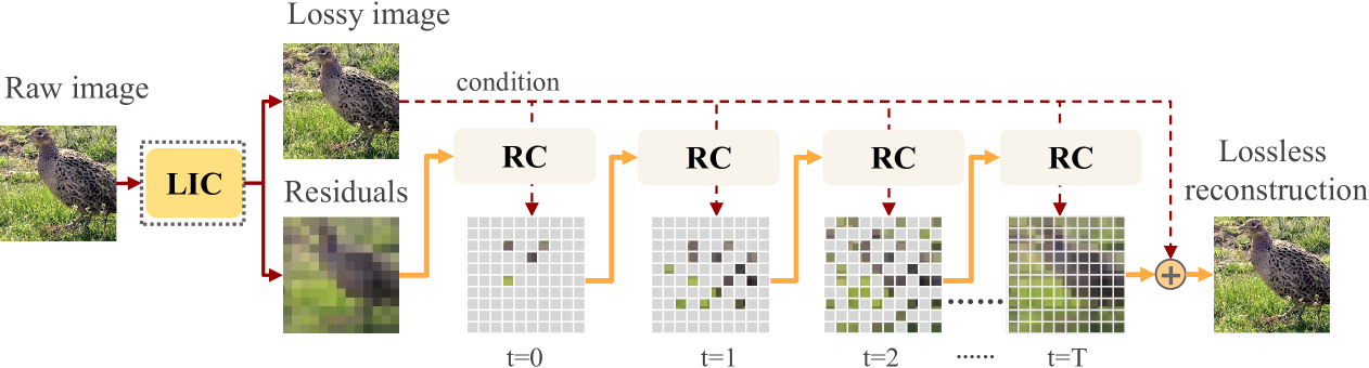
Figure 1. Overview of our masked sampling model. LIC is the learning-based lossy image compressor. RC is the proposed residual compressor. The gray parts are masked residuals during each sampling. For each iteration t, only unmasked residuals are encoded into bitstreams. After iterative $T$ times masked sampling, we finally get the whole residual image and add it to the lossy image to get the raw image.

1. Introduction

For some application scenarios such as remote disease diagnosis and remote sensing, mathematically lossless image compression is essential for image data transmission and storage. In recent years, end-to-end deep lossy (Ballé et al., 2018; He et al., 2022; Cheng et al., 2020), and lossless (Mentzer et al., 2019; Ma et al., 2020; Cao et al., 2020; Hoogeboom et al., 2019; Luo et al., 2023; Mentzer et al., 2020; Bai et al., 2022, 2024; Rhee et al., 2022) image compression have been witnessed with great progresses. They demonstrate superior compression performance to the conventional image codecs and great potential to achieve lower time complexity by efficient parallel computing. Following Shannon’s source coding theorem (Shannon, 1948), the low bound of expected code length is given by the real probability distribution of image data, i.e., the information entropy. Consequently, even the state-of-the-art lossless image compressors only have a 2x $\sim$ 3x compression rate, in contrast to 50x for lossy compression.

The existing learning-based lossless image compression works (Salimans et al., 2017; Mentzer et al., 2020; Bai et al., 2022; Ma et al., 2020) rely heavily on sophisticated auto-regressive models to estimate the probability distribution of pixels conditioned on decoded symbols, achieving remarkable compression with long decoding time. For practicality, recent works LC-FDNET(Luo et al., 2023) and DLPR (Bai et al., 2024) proposed some parallelization mechanisms, such as encoding in the unit of subimage or patch rather than individual pixels. However, regardless of pixel, patch, or subimage as the basic coding unit (CU), these works still strictly encode/decode an image in raster scan order, which is not consistent with the way humans perceive images. Moreover, previous works only consider one-directional contexts, ignoring other contextual dependencies in other directions. The mechanism is suitable for one-dimensional sequential data like texts, but not optimal or efficient for two-dimensional non-sequential images. Recent image diffusion models gradually denoise from a noisy image and finally obtain a clean image. Inspired by this, we treat image coding as a gradual process by masked sampling, which progressively refines the probability distribution of residuals for improved lossless compression. Furthermore, we propose a multi-direction auto-regression framework via masked sampling, which considers the dependencies among previous, current, and future symbols for better probability estimation of residuals in a coarse-to-fine manner. In summary, we follow the idea of deep lossy plus residuals coding for lossless image compression, but the residual coding is performed by iteratively refining the probability estimation. As shown in Figure 1, a lossy image $\hat{X}$ is obtained by a lossy image compressor (LIC), and then the residual $R=X-\hat{X}$ is lossless encoded conditioned on $\hat{X}$ and the contexts (unmasked symbols) by the residual compressor (RC) with $T$ iterations. At each iteration $t$, we sequentially perform: $probability\ estimation\ (P)\to mask\ generation\ (M)\to arithmetic\ coding\ (E)$. Specifically, masks are generated according to the estimated probability distribution, which is used to select partial symbols from the whole residuals for coding. Thus, this process is called masked sampling. During each sampling, the spatial locations of the final symbols for coding are variable and scattered in multi-direction, which makes the probability estimation for the next sampling be conditioned on more direction contexts. Only the symbols with high confidence in their probabilistic predictions are unmasked for the entropy coding. We can adjust the optimization granularity (fineness of the probability estimation) and speed (running time) of the model by controlling the variable T. A bigger T implies a more refined iterative optimization process but a longer running time, and vice versa. As a result, T benefits compromising between compression rate and coding runtime. Moreover, the proposed approach is suitable for the lossless compression of grayscale and color images with a single model since it treats each component separately. In summary, the contributions of this work are three-fold.

• We propose a deep lossless image compression approach via iterative masked sampling and coarse-to-fine auto-regression. Through $T$ times masked sampling, the autoregressive context modeling is extended from one direction to multiple directions and can be progressively conditioned on more contextual dependencies for enhanced performance.

• Scalable lossless image compression is achieved by adjusting T, which controls the granularity and runtime of probability estimation of the residuals.

• The proposed approach is suitable for the compression of grayscale and color images with a single trained model. And it achieves competitive performance on various benchmark datasets.

2. RELATED WORKS

2.1. Hand-crafted Codec

Conventional image codecs exploit hand-crafted image statistics to remove spatial redundancies among neighboring pixels. Specifically, they achieve compression by reducing redundancies with reversible transform coding, prediction coding, and residual coding. The representative works include Discrete Wavelet Transform (DWT) (Mallat, 1989) based JPEG2000 (Taubman et al., 2002), PNG (Boutell, 1997), BPG (Bellard, 2017) and JPEG XL (Alakuijala et al., 2019). These codecs heavily rely on hand-crafted linear transformations and have limitations when representing nonlinear correlations.

2.2. Learnable Lossy Compression

LIC has gained increasing interest due to its superior performance to conventional codecs. Taking advantage of sophisticated deep generative models, existing works (Ballé et al., 2016, 2018; Cheng et al., 2020; He et al., 2022) train Variational AutoEncoder (VAE) to transform raw pixels into compact latent representations (the dimension is set to be much less than the number of pixels), and then model the probability distribution parameters of quantized representations via auto-regressive context models. The probabilities are calculated by a single or mixture distribution model and then are fed to an arithmetic coder to output bitstreams. Arithmetic coding is lossless, but the transform from pixels to latent representations by VAE and the quantization incur information loss. Benefiting from the likelihood-based generative model’s ability to learn the unknown probability distribution of given data, the learning-based lossy image compression achieves high fidelity and a desirable compression ratio. In this work, we integrate a sophisticated lossy image compression, followed by a customized residual coding for lossless image compression.

2.3. Learnable Lossless Compression

The conventional lossless compression of given symbols can usually be solved in two stages: 1) statistical model the probability distribution $\sim p$ of symbols; 2) according to the statistical distribution $\sim p$, encode the symbols into bitstreams with arithmetic coder. Deep generative models are mainly trained to complete the first-stage task. Among them, the pixel-wise autoregressive model, i.e, PixelCNN++ (Salimans et al., 2017) models the distribution as $p(x)=\prod_{i}p(x_{i}|x_{1},\dots,x_{i-1})$. Despite the notable compression rate, its sequential decoding process makes it time-consuming and impractical. The subimage-wise models address this issue by modeling the distribution in a coarse granularity as $p(S_{i})=p(S_{i}|S_{1},\dots,S_{i-1})$. L3C (Mentzer et al., 2019) and SRec (Cao et al., 2020) use convolution layers and average pooling to decompose the image $X$ into subimages ${\{S_{1},S_{2},\dots S_{n}\}}$ of multiple scales, respectively. LC-FDNet (Rhee et al., 2022) performs spatial downsampling (space-to-depth) on image $X$ to obtain subimages with the same scale. However, their compression ratios are inferior to pixel-wise models. iWave++ (Ma et al., 2020) exploits a multi-level lifting scheme (Sweldens, 1996) to learn reversible integer DWT and models the probability of each wavelet subband via PixelCNN++ (Salimans et al., 2017). But subbands are serially decoded and each wavelet coefficient in subband is pixel-by-pixel, making it time-consuming. Joint lossy compression and residual coding models (Mentzer et al., 2020), Near-lossless (Bai et al., 2022) and its extension work DLPR (Bai et al., 2024) derive the probability distribution of an image $X$ conditioned on the lossy reconstruction $\hat{X}$ from traditional codec and learned codec, respectively. In this paper, we also join lossy compression with a few bits and then design a novel residual coding framework to encode the remaining residuals in a coarse-to-fine manner.

3. Methodology

3.1. Overview

We present a lossless image compression framework by integrating lossy image compression with residual coding. As shown in Figure 1, we first obtain a lossy image $\hat{X}$ with the existing lossy image compressor ELIC (He et al., 2022). Secondly, we construct a residual coding system that progressively encodes/decodes residuals by iterative masked sampling. Specifically, we decompose 9-bit residual into 5-bit plane $R_{1:5}$ (MSB) and 4-bit plane $R_{6:9}$ (LSB). In addition, there is a 1-bit flag to signal whether MSB should be encoded. Only when the flag is 1, we need to encode MSB by Run-length Coding (RLE) (Meyr et al., 1974). Next, we encode the LSB with T times masked sampling. At each iteration $t$, we cascade 3 operations: $P\to M\to E$, as shown in Figure 3. The $P$ operator sends the lossy image $\hat{X}$ condition, channel condition $C_{ch}$ and space condition $C_{sp}$ into the proposed probability estimation network $\Phi$ to output $p^{(t)}$, the logits of symbols over all possible values in time $t$. The $M$ operator receives $p^{(t)}$ to generate a mask matrix $M\in R^{H\times w}$, which is used to select the symbols to be encoded (the red points of Mask in Figure 2) in time $t$, which are subsequently encoded into the bitstream by the operator $E$. After $T$ iterations, $R$ is fully encoded.

Existing lossless image compression works mainly use integrated color components as input and are incapable of supporting grayscale images with a single model. In contrast, our model is more flexible and compatible with grayscale images and color images with a single-trained model. To support multiple format inputs, we separately process each image component with the above pipeline. To accelerate coding, we run each component’s network in parallel during inference.

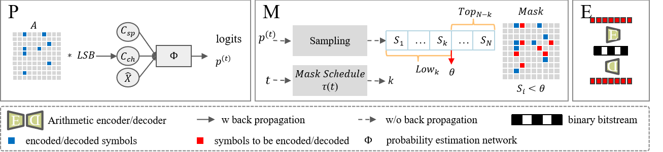
Figure 2. Main components of the proposed framework RC via $T$ times masked sampling.

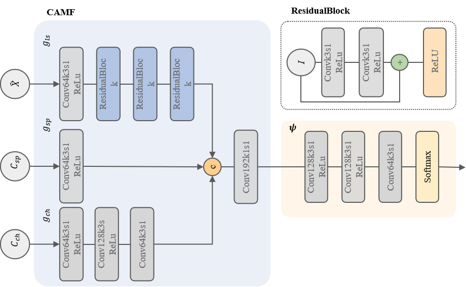
Figure 3. Detailed architecture of the residual probability estimation network $\Phi$ .

3.2. Lossy Compression

Our compression framework exhibits compatibility with arbitrary lossy image codecs. For experimental validation, we adopt the well-established end-to-end learned image compressor ELIC (He et al., 2022), which synergistically combines a hyperprior model with a context model to achieve state-of-the-art rate-distortion performance.

3.3. Residual Compression

Since the superiority of LIC, the theoretical interval [-255, 255] of $R=X-\hat{X}$ can hardly be filled up in practice. We linearly transform and decompose the residuals into high 5-bit

(1) $$MSB=\left\lfloor\frac{R-R_{min}}{2^{4}}\right\rfloor$$

and the low 4-bit plane (LSB)

(2) $$LSB=(R-R_{min})\bmod\ {2^{4}}.$$

In particular, when the offset residual ${R-R_{min}}$ completely falls in the range of [0,63], MSB is all 0, meaning there is no information to be compressed. Therefore, setting a 1-bit $flag$ can greatly simplify computation and storage. MSB’s sparsity arising from the narrow range of residuals makes it unsuitable and uneconomical for modeling through neural networks. Hence, we choose simple and straightforward RLE (Meyr et al., 1974) to encode MSB when $flag=1$.

LSB mainly contains visually important data and contributes to finer textual details. Consequently, we compress it with the designed neural model RC, comprising three operations as shown in Figure 3. The pipeline for coding the LSB is summarized as the following three steps.

Softmax-likelihood Probability estimation. We employ the flexible softmax likelihood-based non-parametric probability model $\Phi$, as shown in Figure 3. $\Phi$ is composed of the backbone Context-aware Multi-domain Fusion Module (CAMF) and the probability predictor $\psi$. A forward of $\Phi$ outputs the probability mass function (PMF) of whole LSB of $R$, namely logits $p^{(t)}\in{R^{H\times W\times 64}}$ on possible value for each symbol in time $t$. The derived logits share height and width with $R$, and the channels are 64. CAMF integrates information from three pipelines: lossy reconstruction prior $\hat{X}$, spatial context $C_{sp}$, and channel context $C_{ch}$. In previous works, a spatial context often refers to the currently observable neighbors of $i-th$ coding symbols. It is limited as symbols before $r_{i}$ in a predefined raster scan order (i.e., from left to right line by line), namely $r_{<i}=\{r_{1},\dots,r_{i-1}\}$. Our method expands them to symbols coming from all directions,

(3) $$C_{sp}=\{r_{j}|j\in N,A_{j}=1\},$$

where $A$ is the binary matrix plotted in Figure LABEL:fig and $A_{j}=1$ indicates the encoded/decoded symbols (blue points).

The spatial context $C_{sp}$ is perceived by the spatial context model $g_{sp}$, and rich neighborhood information $F_{sp}$ is extracted to promote the PMF estimation of symbols.

(4) $$F_{sp}=g_{sp}(C_{sp}).$$

Channel context $C_{ch}$ refers to the observable neighboring components. For chrominance components, it leverages cross-channel correlations:

(5) $$F_{ch}=g_{ch}(C_{ch}).$$

Lossy reconstruction prior $F_{ls}$ is extracted from the lossy image $\hat{X}$ by the lossy context model $g_{ls}$, composed of continuously stacked residual blocks for increasing the receptive field.

(6) $$F_{ls}=g_{ls}(\hat{X}).$$

The fusion module combines these contexts via $1\times 1$ convolution followed by softmax-based probability prediction:

(7) $$p^{(t)}=\text{Softmax}\left(\psi\left(\text{Conv}{1\times 1}(F_{sp},F_{{ch}},F_{{ls}})\right)\right)$$

where $\psi$ implements lightweight (64-channel) convolution for parameter efficiency. It directly outputs 64 numbers per symbol describing the logits on the 64 potential values for each symbol.

Mask generator. At time $t$, we only encode $k$ symbols with high-confidence probability prediction. We sample a value matrix $V^{(t)}\in R^{H\times W}$ by the probability $p^{(t)}$ predicted by $\Phi$ and calculate a confidence score matrix $S^{(t)}\in R^{H\times W}$, which indicates the confidence of probability prediction in each spatial location (i,j). The $k$ locations with lower scores ($S^{(t)}_{i,j}\leq\theta$) are masked ($M^{(t)}_{i,j}=1$). The $N-k$ locations with $S^{(t)}_{i,j}>\theta$ (the blue and red point in Mask in the Figure 3) are reserved ($M^{(t)}_{i,j}=0$).

The training objective of $\Phi$ minimizes masked cross-entropy of predicted distribution $p$ and the marginal distribution $\tilde{p}$ of symbols to be encoded:

(8) $$\begin{split}L_{M^{(t)}_{i,j}=1}=\sum_{r_{i,j}\in R}\tilde{p}(r_{i,j})\log p^{(t)}(r_{i,j}).          \end{split}$$

Note that during training, the model only performs the single-pass mask implementation that enables efficient training without iterative refinement.

Arithmetic coding. After operator $M$, we obtain the locations of symbols with high confidence scores. We maintain an anchor matrix $A$ to record the location of encoded/decoded symbols (blue points), which is updated cumulatively in each sampling. We use torchac(Mentzer et al., 2019) as an arithmetic coder to encode/decode the red points.

3.4. Iterative masked sampling

Motivated by the MaskGIT (Chang et al., 2022) that iteratively generates the latent tokens by a mask schedule, we adapt iterative masked sampling to residual compression in the pixel domain. As described in Algorithm 1, at initilization ($t=1$), we initialize the $A=0$ and $M^{(}1)=1$, representing no known symbols for context. At iteration $t$, we first compute $k=\tau(t)\times H\times W$, the number of symbols to be masked according to the mask scheduler $\tau(t)$ and the total number of pixels $H\times W$ .Secondly, we sample $V^{(t)}$ by probability $p^{(t)}$ to replace the unknown symbols ($A_{i,j}=0$) with $V^{(t)}_{i,j}$. We get the probability $p^{(t)}_{i,j,V^{(t)}_{i,j}}$, a scalar representing the probability of the location (i,j) valued $V^{(t)}_{i,j}$, which is then used to compute a score matrix $S^{(t)}$ by

(9) $$S^{(t)}_{i,j}=\left\{\begin{matrix}p^{(t)}_{i,j,V^{(t)}_{i,j}}+\beta*z,z\sim N(0,1)&ifA_{i,j}=0\\ 1&ifA_{i,j}=1,\end{matrix}\right.$$

where $\beta$ is a temperature factor to regulate the degree of added random noise $z$. The $k$ lowest-score positions are masked ($M^{(t)}_{(i,j)}$) for subsequent refinement. The decoding is described in Algorithm 2. The T-step iterative encoding/decoding process progressively converts coarse initial estimates into fine-grained reconstructions.

3.5. Coarse to Fine and Multi-directional Autoregression

Following the raster scan ordering, pixel/subimage-based autoregressive models sequentially decode an image with slow speeds. Usually, these autoregressive models employ $k\times k$ masked convolution to mask out further information, ensuring strictly causal dependency - the conditional probability estimation of current symbols only depends on decoded symbols. In this paper, we propose a coarse-to-fine and multi-directional auto-regressive context model. The mask scheduling function $\tau(t)$ controls the coarse-to-fine refinement process through following critical properties. $\tau(1)=1$ initiates full masking (coarse estimation) and $\tau(T)=0$ ensures complete refinement (fine details). $\tau(t)\downarrow$ as $t$ increases maintains progressive information accumulation, where probability prediction is more confident and fine-grained because of incorporating more contextual information. We finally take the monotonically decreasing and positive part of the cosine function:

(10) $$\tau(t)=\left\{\begin{matrix}cos(\frac{t\pi}{2T})&if\enspace inference\\ cos(\frac{\epsilon\pi}{2})&if\enspace training\end{matrix}\right.$$

where $\epsilon\in(0,1)$ is a random number.

When training, we only perform one masked sampling for each component. The $k$ is decided by the random ratio $\epsilon$. We generate $k$ positions (i,j) with the lowest values from a matrix obeying a uniform distribution $U\sim(0,1)$ and masks them $M_{i,j}=1$. When encoding/decoding, we iteratively sample T times, and the $k$ and $M^{(t)}$ are calculated as Algorithm 1 and Algorithm 2. At each time $t$, the probability modeling of the unknown symbols is conditioned on the encoded/decoded symbols in previous times $<t$,

(11) $$p^{(t)}_{{A_{i,j}=0}}(x)=p^{(t)}(x_{i,j}|x_{m,n},A_{m,n}=1)$$

The known symbols from multiple directions facilitate effectively learning the pattern of residual by T iterations.

Algorithm 1 algorithm of encoding

0: $T$, $H,W$, $\hat{X}$,$\beta$,$R$$\quad A\leftarrow\textbf{0}$, $M^{(1)}\leftarrow\textbf{1}$ Set the random number seed;

0: $bitstream$

1: for $t=1$ to $T$ do

2:  $k=\tau(t)\times H\times W$  

3:  $C_{sp}=A\cdot R$

4:  if $C_{ch}=\emptyset$  then

5:   $C_{ch}=C_{sp}$

6:  end if

7:  $p^{(t)}=Softmax(\psi(g_{ls}(\hat{X}),g_{sp}(C_{sp}),g_{ch}(C_{ch}))$

8:  $V^{(t)}\leftarrow$ probabilistic sampling from $by\sim p^{(t)}$

9:  if $A_{i,j}=0$ then

10:   $\tilde{p}^{(t)}_{i,j}=inf$

11:  else

12:   $\tilde{p}^{(t)}_{i,j}=p^{(t)}(i,j,V^{(t)}_{i,j})$

13:  end if

14:  $S^{(t)}_{i,j}=\log{\tilde{p}^{(t)}(i,j)}+\beta*z,z\sim N(0,1)$

15:  Flatten $S^{(t)}$ and sort it in ascending order

16:  $\theta=S^{(t)}[k]$

17:  if $S^{(t)}_{i,j}<\theta$ then

18:   $M^{(t)}_{i,j}=1$

19:  else

20:   $M^{(t)}_{i,j}=0$

21:  end if

22:  $symbol=(A\oplus M^{(t)})\cdot R,pdf=(A\oplus M^{(t)})\cdot p^{(t)}$

23:  $bitstream+=E(symbol,pdf)$

24:  $A=A||M^{(t)}$

25: end for

26: return  $bitstream$

Algorithm 2 algorithm of decoding

0: $bitstream,T$, $H,W$, $\hat{X}$,$\beta$,$\quad A\leftarrow\textbf{0}$, $M^{(1)}\leftarrow\textbf{1},R\leftarrow\textbf{0}$ Set the random number seed.

0: $R$

1: for $t=1$ to $T$ do

2:  $k=\tau(t)\times H\times W$, $C_{sp}=A\cdot R$

3:  if $C_{ch}=\emptyset$  then

4:   $C_{ch}=C_{sp}$

5:  end if

6:  $p^{(t)}=Softmax(\psi(g_{ls}(\hat{X}),g_{sp}(C_{sp}),g_{ch}(C_{ch}))$

7:  $V^{(t)}\leftarrow$ probabilistic sampling by$\sim p^{(t)}$

8:  calculate $S^{(t)}_{i,j}$ by Equation 9

9:  Flatten $S^{(t)}$ and sort it in ascending order, $\theta=S^{(t)}[k]$

10:  if $S^{(t)}_{i,j}<\theta$ then

11:   $M^{(t)}_{i,j}=1$

12:  else

13:   $M^{(t)}_{i,j}=0$

14:  end if

15:  $pdf=(A\oplus M^{(t)})\cdot p^{(t)}$

16:  $R_{(A\oplus M^{(t)})=1}=D(bitstream,pdf)$

17:  $A=A||M^{(t)}$

18: end for

19: return  $R$

3.6. Rate-Latency Scalability

Differing from existing approaches in computational scalability, our framework introduces tunable rate-latency tradeoffs through adaptive iteration control. DLPR (Bai et al., 2024) splits the $H\times W$ image into multiple non-overlapping $P\times P$ patches and codes all patches in parallel. Since the context of each pixel is limited to a patch, the $H\times W$ times sequential context computations can be finished with $P^{2}$ times forward computation latency, a significant reduction compared with $H\times W$ times runtime of PixelCnn++ (Salimans et al., 2017). In contrast, our method only costs $T\in\{1,2,\dots,12\}$ times forward computation latency. $P^{2}$($P=64$ in DLPR) is usually greater than $T$. During each sampling, the probability of all symbols in $R$ is generated simultaneously in parallel. As shown in Figure 4, the time overhead of the three operators $P,M,E$ in each sampling are denoted as $t_{P},t_{M},t_{e}$. When encoding, we minimize runtime by cascading three operators. Specifically, once the $M$ operator is executed at time $t-1$, the $P$ operator at time $t$ can commence without waiting for the completion of the $E$ operator at $t-1$. As a result, we get a latency of $T*(t_{P}+t_{M})+t_{E}$. When decoding, the probability estimation operator $P$ at time $t+1$ can only be operated after the arithmetic decoding operator $E$ at time $t$ is completed. Consequently, decoding requires strict serialization with a latency of $T*(t_{P}+t_{M}+t_{E})$. In addition, the iteration count T controls the rate-latency tradeoffs. A larger T corresponds to finer coding, lower bit rates, and increased latency, while a smaller T leads to coarser coding, higher bit rates, and decreased latency, and vice versa. We can flexibly trade off the rate and latency of compression by fine-tuning an appropriate T , which is a significant advantage of our method over other lossless compression methods.

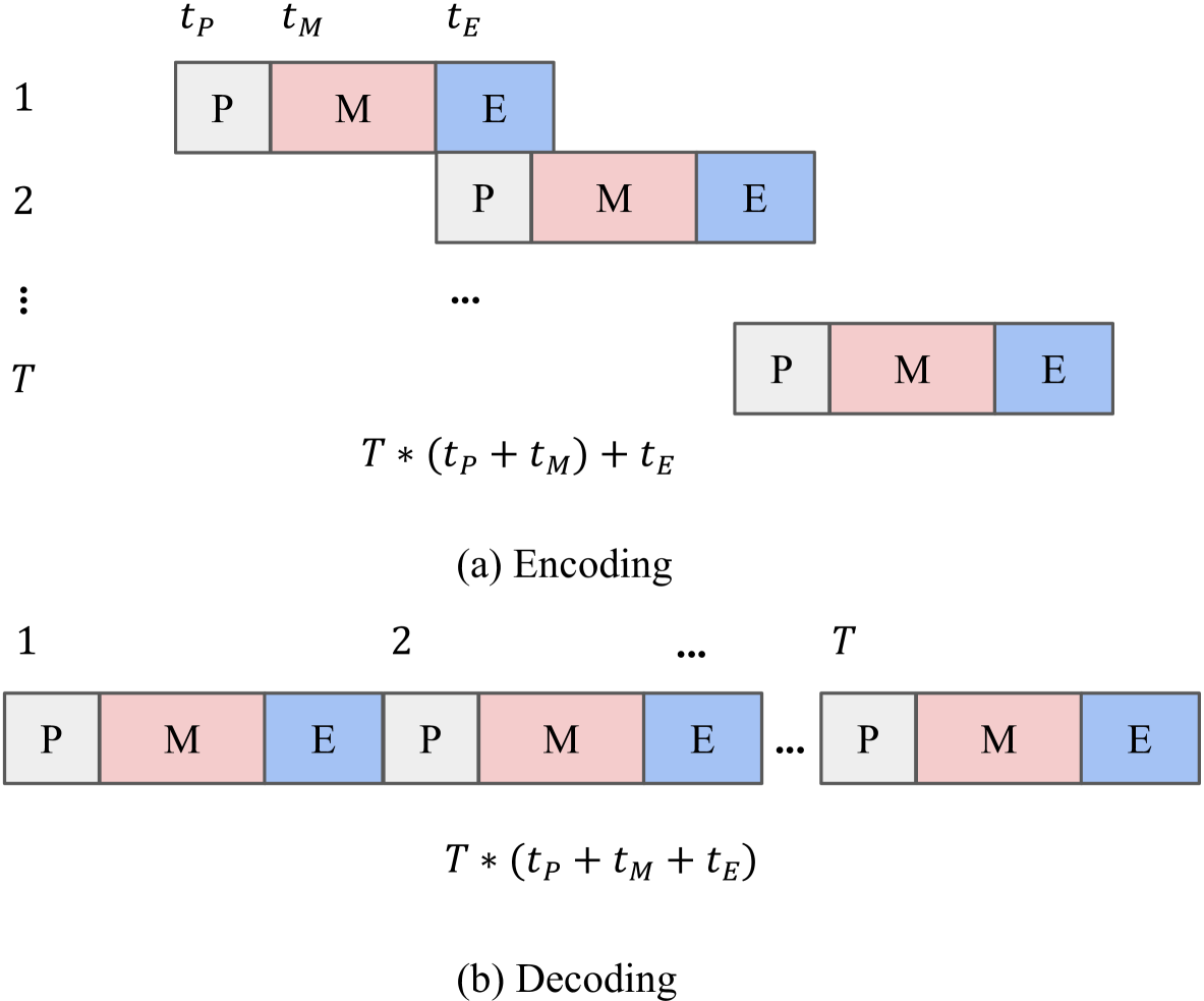
Figure 4. Latency analysis

4. Experiments

Table 1. Lossless image compression performance (bpp) of our proposed coding system, compared with other lossless image codecs on all evaluation sets. The bpp of our method in the table contains the sum of all parts. The best performance is highlighted in bold, and the second-best performance is denoted with *. “-” indicates that the result is not available because of the availability of code or training weights

Codec	ImageNet64	Open Images	CLIC.m	CLIC.p	DIV2K	Kodak
PNG (Boutell, 1997)	17.22	12.09	11.79	11.79	12.69	13.05
JPEG2000 (Taubman et al., 2002)	15.57	9.18	8.13	8.79	8.97	9.57
WebP (Version, 2000)	13.92	9.09	8.19	8.7	9.33	9.54
BPG (Bellard, 2017)	13.26	12.98	8.52	9.24	9.84	10.14
FLIF (Sneyers and Wuille, 2016)	13.62	8.61	7.44	8.16	8.73	11.7
JPEG-XL (Alakuijala et al., 2019)	14.82	8.28	7.2	8.19	8.49	$8.61^{*}$
JPEG-LS	13.35	-	7.59	8.46	8.97	9.48
LCIC (Kim and Cho, 2013)	-	-	7.88	9.02	9.35	-
L3C (Mentzer et al., 2019)	13.26	8.97	7.92	8.82	9.27	9.78
SRec (Cao et al., 2020)	12.87	$8.10^{*}$	7.94	9.12	9.30	9.93
RC (Mentzer et al., 2020)	-	-	7.62	8.79	9.24	-
IDF (Hoogeboom et al., 2019)	11.7	8.28	-	-		-
IDF+	11.43	-	-	-	-	-
Near-Lossless (Bai et al., 2022)	-	-	7.53	7.98	8.43	9.12
iwave++ (Ma et al., 2020)	12.5		10.51	10.34		11.87
Bit-Swap (Kingma et al., 2019)	15.18	-	-	-	-	-
HiLLoC (Townsend et al., 2019)	11.7	-	-	-	-	-
iFlow (Zhang et al., 2021)	$10.95^{*}$	-	6.78	$7.32$	7.71	-
DLPR (Bai et al., 2024)	11.07	7.47	6.48	7.14	$7.65^{*}$	8.58
Ours (T=12)	10.14	8.19	6.98	7.94	7.62	8.97

Table 2. Average running time (s) of other codecs and ours ($T=12$) on Kodak ($728\times 512$) dataset.

runtime(s)	JPEG-LS	BPG	FLIF	JPEG-XL	L3C	Minnen	iWave++	DLPR	Ours
Encode	0.12	2.38	0.9	0.73	8.17	2.55	158	1.26	1.12
Decode	0.12	0.13	0.16	0.08	7.89	5.18	-	1.8	3.54

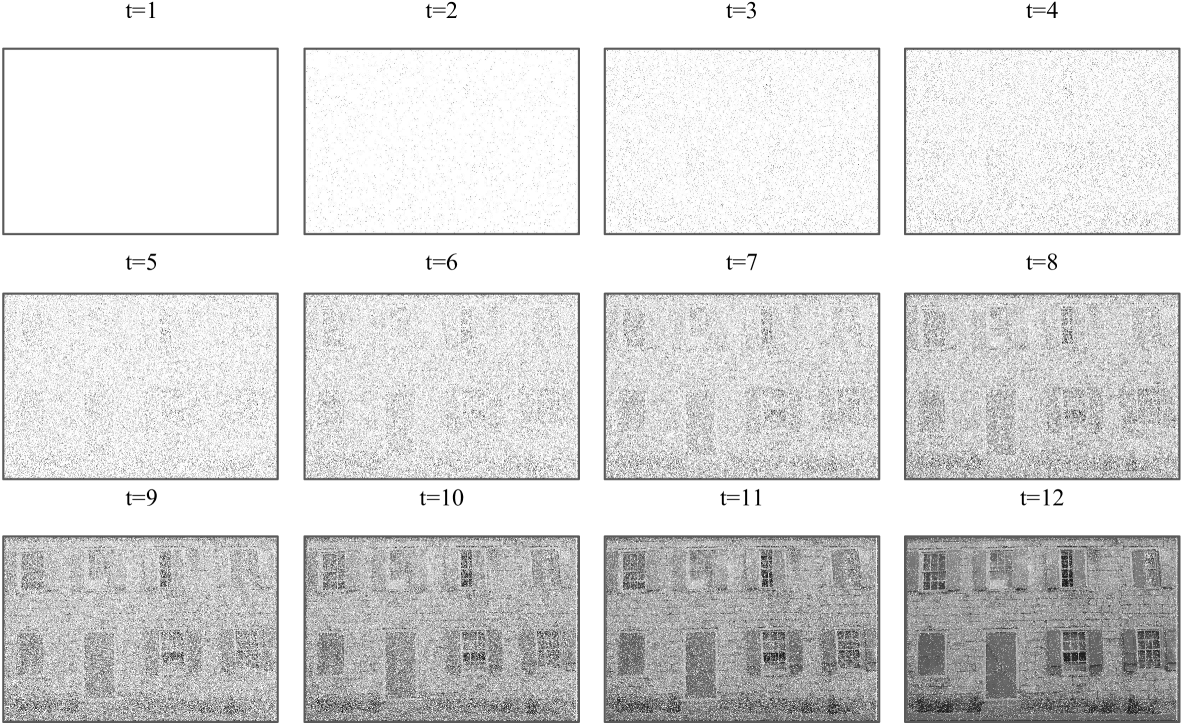
Figure 5. Visualization of coarse-to-fine auto-regressive models. We show the context conditioned on at time $t$, i.e., the encoded/decoded symbols. Unknown symbols are replaced by white pixel dots.

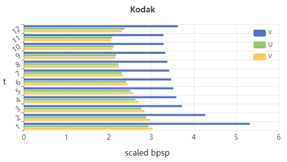
Figure 6. Comparison results (scaled bpsp) for each component and each iteration of the Kodak dataset. The scaled bpsp is the total bits per iteration $t$ divided by the number of coded symbols per iteration $t$ rather than the total number of pixels $N$.

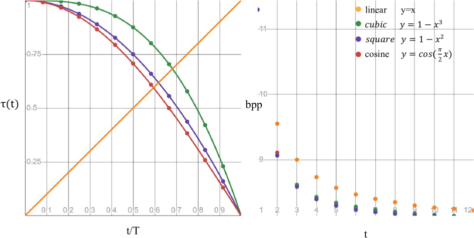
Figure 7. Choices of Mask Scheduling Functions $\tau(t)$ during inference. The right figure shows the compression results (bpp) on the Kodak dataset with different mask functions ($T=12,\beta=10.5$).

4.1. Experimental Setup

Datasets. We conduct a comprehensive evaluation across six benchmark datasets representing diverse image characteristics.

• Kodak: Kodak dataset consists of 24 uncompressed $768\times 512$ color image.

• Open Images: The 500 color images selected from the Open Images validation dataset (Krasin et al., 2017).

• DIV2K: DIV2K high resolution validation dataset (Agustsson and Timofte, 2017) consists of 100 2K color images.

• CLIC.p: CLIC professional validation dataset (Toderici et al., 2020) consists of 41 color images, of which most are in 2K resolution.

• CLIC.m: CLIC mobile validation dataset (Toderici et al., 2020) consists of 61 2K resolution color images.

• ImageNet64: ImageNet64 validation dataset is a downsampled variant of the ImageNet validation dataset, consisting of 50000 images of size $64\times 64$.

Training. We train our network on 18000 images chosen from the ImageNet (Deng et al., 2009) validation set. During training, we randomly rotate the images and crop patches of the size $256\times 256$. The Adam optimizer (Kingma and Ba, 2014) is used, with the batch-size 16 and initial learning rate $1\times 10^{-4}$ for 600 epochs. For the sake of stability, we apply gradient clipping (clip max norm =1.0) and decay learning rate to $1\times 7.5^{-5}$ for the last 300 epochs. We use the ELIC (He et al., 2022) as our lossy image compressor and freeze it during our training of the residual compressor. Our coding system is trained and evaluated on Intel(R) Core(TM) i7-9800X CPU @ 3.80GHz, 62G RAM, NVIDIA RTX2080 Ti. We set the same random seed to ensure that each random operation gets replicable results. We set $T=12,\beta=10.5$, leading to the best lossless image compression performance.

4.2. Evaluation Results

We evaluate the lossless image compression performance of our coding system with the bit per pixel (bpp). Like DLPR, we also compare with eight traditional lossless image codecs: including PNG (Boutell, 1997), JPEG-LS (Weinberger et al., 2000), CALIC (Wu and Memon, 1997), JPEG2000 (Taubman et al., 2002), LCIC (Kim and Cho, 2013), WebP (Version, 2000), BPG (Bellard, 2017), FLIF (Sneyers and Wuille, 2016) and JPEG-XL (Alakuijala et al., 2019), and 11 recent learning-based lossless image compression methods including: L3C (Mentzer et al., 2019), RC (Mentzer et al., 2020)], Bit-Swap (Kingma et al., 2019), HiLLoC (Townsend et al., 2019), IDF (Hoogeboom et al., 2019) [14], IDF++ (Berg et al., 2020), LBB (Ho et al., 2019), iFlow (Zhang et al., 2021), iWave (Ma et al., 2020), DLPR (Bai et al., 2024) and its predecessors Near-Lossless (Bai et al., 2022).

As reported in Table 1, our approach achieves 7.62 bpp, outperforming the previous best DLPR (7.65 bpp) by 0.39%. This improvement stems from our multidirectional context aggregation that better captures long-range dependencies in high-resolution images. For the ImageNet64 dataset ($64\times 64$), we set a new benchmark of 10.14 bpp - an 8.4% reduction compared to DLPR’s 11.07 bpp. This demonstrates the exceptional effectiveness of our method on small images. For other datasets, our method is inferior to DLPR performance but comparable to traditional codecs. The above results demonstrate that our coding system achieves competitive lossless image compression performance and can be effectively generalized to images of various domains.

4.3. Computational Efficiency

We measure the average runtime required for encoding/decoding the Kodak dataset ($768\times 512$). As reported in Table 2, our coding system has superiority over other learned codecs when encoding due to the parallel processing of each component and the pipelined cascade of three operators at each sampling. Since the dependencies between components must be handled serially, our decoding time is longer than DLPR but still comparable to the remaining learning codecs. In detail, for the loss image $\hat{X}$, the average encoding and decoding times are 193 ms and 317 ms. For the residual image $R$, three components can be encoded in parallel, and the total encoding time is 927 ms. The decoding time is 3228 ms due to the serial processing of three components. Together with the lossy image, the total encoding and decoding times are 1120 ms and 3545 ms.

4.4. Coarse-to-fine modeling

We quantitatively and qualitatively demonstrate the effectiveness of masked sampling in enhancing compression performance. We first report the compression results of each component and iteration in Figure 6. We observe that the compression effects of each component enhance with the increase of t. This is straightforward since more information from more directions becomes available as the iteration proceeds. From the perspective of channels, better compression is presented in the order of $Y\to U\to V$. This can be attributed to our channel context model capturing more dependencies between color components. Subsequently, we visualize the progressive contexts at each iteration $t$ in Figure 5. The reconstructed image becomes clearer over time $t$, which visually demonstrates the learning and enhancement process of our model.

4.5. Ablation Study

Different mask schedulers. We find that the compression bitrate is affected by the mask schedule function $\tau(t)$. As visualized in Figure 7, we consider several functions $\tau(t)$ that satisfy the constraint: $\tau(t)\in[0,1]and\enspace\tau\downarrow$. The $\tau(t)$ controls the mask ratio in each iteration and influences the $k=\tau(T)=\tau(t)*N$. We observe that the cosine function and square function perform better overall. The linear function performs the worst because it is incapable of scheduling the $k$ well enough to accommodate our coarse-to-fine process.

Rate-latency tradeoff Analysis . We show the results of adjusting variable T to trade off bitrate and coding runtime in Table 3. As $T$ increases, the bpp decreases, and the coding runtime increases. When T increases to a certain extent, the reduction of bpp slows down and the growth of runtime accelerates. Therefore, we cannot continue to increase $T$ to reduce bpp at this point, which will bring a large increase in running time. All things considered, $T=12$ is a good balance between rate and runtime.

Table 3. The effects of different T for bpp and runtime (s) on Kodak with cosine mask schedule function and temperature coefficient $\beta=10.5$ (only including the residual part of image).

	1	2	5	8	12	32
bpp	11.30	9.11	8.30	8.17	8.11	8.04
Encode (s)	0.272	0.380	0.458	0.733	0.933	2.451
Decode (s)	0.760	1.236	1.368	2.189	3.246	8.758

5. Conclusion

In this paper, we have proposed a scalable lossless image compression framework that supports single/multiple-component images with a single-trained model. Our framework consists of a lossy image compressor and a specialized residual compressor, which decomposes the whole residual compression into $T$ times masked sampling. With the mask design, we propose the multiple-direction auto-regressive context model for probability estimation of residual. The $T$ times masked sampling proceeds in a coarse-to-fine manner, which progressively refines the probability estimation of residual. Furthermore, our framework enables tunable rate-latency tradeoffs through adaptive iteration times $T$. Experiments demonstrate that our coding framework implements competitive lossless compression performance with practical complexity on various full-resolution images.

5.1. Discussion

Due to the training cost, we freeze the lossy compression network and only train the proposed residual network. If these models are trained jointly, the compression performance will be further improved. In addition, how to train the residual compressor generalized to residuals of different distributions produced by various lossy compression networks, which is also the direction of our efforts.

References

- (1)
- Agustsson and Timofte (2017) Eirikur Agustsson and Radu Timofte. 2017. Ntire 2017 challenge on single image super-resolution: Dataset and study. In Proceedings of the IEEE conference on computer vision and pattern recognition workshops. 126–135.
- Alakuijala et al. (2019) Jyrki Alakuijala, Ruud Van Asseldonk, Sami Boukortt, Martin Bruse, Iulia-Maria Comșa, Moritz Firsching, Thomas Fischbacher, Evgenii Kliuchnikov, Sebastian Gomez, Robert Obryk, et al. 2019. JPEG XL next-generation image compression architecture and coding tools. In Applications of Digital Image Processing XLII, Vol. 11137. SPIE, 112–124.
- Bai et al. (2022) Yuanchao Bai, Xianming Liu, Kai Wang, Xiangyang Ji, Xiaolin Wu, and Wen Gao. 2022. Deep Lossy Plus Residual Coding for Lossless and Near-lossless Image Compression. arXiv preprint arXiv:2209.04847 (2022).
- Bai et al. (2024) Yuanchao Bai, Xianming Liu, Kai Wang, Xiangyang Ji, Xiaolin Wu, and Wen Gao. 2024. Deep lossy plus residual coding for lossless and near-lossless image compression. IEEE Transactions on Pattern Analysis and Machine Intelligence (2024).
- Ballé et al. (2016) Johannes Ballé, Valero Laparra, and Eero P Simoncelli. 2016. End-to-end optimized image compression. arXiv preprint arXiv:1611.01704 (2016).
- Ballé et al. (2018) Johannes Ballé, David Minnen, Saurabh Singh, Sung Jin Hwang, and Nick Johnston. 2018. Variational image compression with a scale hyperprior. arXiv preprint arXiv:1802.01436 (2018).
- Bellard (2017) F Bellard. 2017. BPG image format (http://bellard. org/bpg/).
- Berg et al. (2020) Rianne van den Berg, Alexey A Gritsenko, Mostafa Dehghani, Casper Kaae Sønderby, and Tim Salimans. 2020. Idf++: Analyzing and improving integer discrete flows for lossless compression. arXiv preprint arXiv:2006.12459 (2020).
- Boutell (1997) Thomas Boutell. 1997. Png (portable network graphics) specification version 1.0. Technical Report.
- Cao et al. (2020) Sheng Cao, Chao-Yuan Wu, and Philipp Krähenbühl. 2020. Lossless image compression through super-resolution. arXiv preprint arXiv:2004.02872 (2020).
- Chang et al. (2022) Huiwen Chang, Han Zhang, Lu Jiang, Ce Liu, and William T Freeman. 2022. Maskgit: Masked generative image transformer. In Proceedings of the IEEE/CVF Conference on Computer Vision and Pattern Recognition. 11315–11325.
- Cheng et al. (2020) Zhengxue Cheng, Heming Sun, Masaru Takeuchi, and Jiro Katto. 2020. Learned image compression with discretized gaussian mixture likelihoods and attention modules. In Proceedings of the IEEE/CVF conference on computer vision and pattern recognition. 7939–7948.
- Deng et al. (2009) Jia Deng, Wei Dong, Richard Socher, Li-Jia Li, Kai Li, and Li Fei-Fei. 2009. Imagenet: A large-scale hierarchical image database. In 2009 IEEE conference on computer vision and pattern recognition. Ieee, 248–255.
- He et al. (2022) Dailan He, Ziming Yang, Weikun Peng, Rui Ma, Hongwei Qin, and Yan Wang. 2022. Elic: Efficient learned image compression with unevenly grouped space-channel contextual adaptive coding. In Proceedings of the IEEE/CVF Conference on Computer Vision and Pattern Recognition. 5718–5727.
- Ho et al. (2019) Jonathan Ho, Evan Lohn, and Pieter Abbeel. 2019. Compression with flows via local bits-back coding. Advances in Neural Information Processing Systems 32 (2019).
- Hoogeboom et al. (2019) Emiel Hoogeboom, Jorn Peters, Rianne Van Den Berg, and Max Welling. 2019. Integer discrete flows and lossless compression. Advances in Neural Information Processing Systems 32 (2019).
- Kim and Cho (2013) Seyun Kim and Nam Ik Cho. 2013. Hierarchical prediction and context adaptive coding for lossless color image compression. IEEE Transactions on image processing 23, 1 (2013), 445–449.
- Kingma and Ba (2014) Diederik P Kingma and Jimmy Ba. 2014. Adam: A method for stochastic optimization. arXiv preprint arXiv:1412.6980 (2014).
- Kingma et al. (2019) Friso Kingma, Pieter Abbeel, and Jonathan Ho. 2019. Bit-swap: Recursive bits-back coding for lossless compression with hierarchical latent variables. In International Conference on Machine Learning. PMLR, 3408–3417.
- Krasin et al. (2017) I Krasin, T Duerig, N Alldrin, V Ferrari, S Abu-El-Haija, A Kuznetsova, H Rom, J Uijlings, S Popov, A Veit, et al. 2017. Openimages: a public dataset for large-scale multi-label and multi-class image classification. Dataset (2017).
- Luo et al. (2023) Jixiang Luo, Shaohui Li, Wenrui Dai, Chenglin Li, Junni Zou, and Hongkai Xiong. 2023. Learned Lossless Compression for JPEG via Frequency-Domain Prediction. arXiv preprint arXiv:2303.02666 (2023).
- Ma et al. (2020) Haichuan Ma, Dong Liu, Ning Yan, Houqiang Li, and Feng Wu. 2020. End-to-end optimized versatile image compression with wavelet-like transform. IEEE Transactions on Pattern Analysis and Machine Intelligence 44, 3 (2020), 1247–1263.
- Mallat (1989) Stephane G Mallat. 1989. A theory for multiresolution signal decomposition: the wavelet representation. IEEE transactions on pattern analysis and machine intelligence 11, 7 (1989), 674–693.
- Mentzer et al. (2019) Fabian Mentzer, Eirikur Agustsson, Michael Tschannen, Radu Timofte, and Luc Van Gool. 2019. Practical full resolution learned lossless image compression. In Proceedings of the IEEE/CVF conference on computer vision and pattern recognition. 10629–10638.
- Mentzer et al. (2020) Fabian Mentzer, Luc Van Gool, and Michael Tschannen. 2020. Learning better lossless compression using lossy compression. In Proceedings of the IEEE/CVF Conference on Computer Vision and Pattern Recognition. 6638–6647.
- Meyr et al. (1974) H Meyr, H Rosdolsky, and T Huang. 1974. Optimum run length codes. IEEE transactions on Communications 22, 6 (1974), 826–835.
- Rhee et al. (2022) Hochang Rhee, Yeong Il Jang, Seyun Kim, and Nam Ik Cho. 2022. LC-FDNet: Learned Lossless Image Compression with Frequency Decomposition Network. In Proceedings of the IEEE/CVF Conference on Computer Vision and Pattern Recognition. 6033–6042.
- Salimans et al. (2017) Tim Salimans, Andrej Karpathy, Xi Chen, and Diederik P Kingma. 2017. Pixelcnn++: Improving the pixelcnn with discretized logistic mixture likelihood and other modifications. arXiv preprint arXiv:1701.05517 (2017).
- Shannon (1948) Claude Elwood Shannon. 1948. A mathematical theory of communication. The Bell system technical journal 27, 3 (1948), 379–423.
- Sneyers and Wuille (2016) Jon Sneyers and Pieter Wuille. 2016. FLIF: Free lossless image format based on MANIAC compression. In 2016 IEEE international conference on image processing (ICIP). IEEE, 66–70.
- Sweldens (1996) Wim Sweldens. 1996. The lifting scheme: A custom-design construction of biorthogonal wavelets. Applied and computational harmonic analysis 3, 2 (1996), 186–200.
- Taubman et al. (2002) David S Taubman, Michael W Marcellin, and Majid Rabbani. 2002. JPEG2000: Image compression fundamentals, standards and practice. Journal of Electronic Imaging 11, 2 (2002), 286–287.
- Toderici et al. (2020) George Toderici, Wenzhe Shi, Radu Timofte, Lucas Theis, Johannes Balle, Eirikur Agustsson, Nick Johnston, and Fabian Mentzer. 2020. Workshop and challenge on learned image compression (clic2020). In CVPR.
- Townsend et al. (2019) James Townsend, Thomas Bird, Julius Kunze, and David Barber. 2019. Hilloc: Lossless image compression with hierarchical latent variable models. arXiv preprint arXiv:1912.09953 (2019).
- Version (2000) WebEngines Blazer Platform Version. 2000. 1.0 hardware reference guide, xp-002202892, network engines. Inc., Jun 1, 92 (2000), 6.
- Weinberger et al. (2000) Marcelo J Weinberger, Gadiel Seroussi, and Guillermo Sapiro. 2000. The LOCO-I lossless image compression algorithm: Principles and standardization into JPEG-LS. IEEE Transactions on Image processing 9, 8 (2000), 1309–1324.
- Wu and Memon (1997) Xiaolin Wu and Nasir Memon. 1997. Context-based, adaptive, lossless image coding. IEEE transactions on Communications 45, 4 (1997), 437–444.
- Zhang et al. (2021) Shifeng Zhang, Ning Kang, Tom Ryder, and Zhenguo Li. 2021. iflow: Numerically invertible flows for efficient lossless compression via a uniform coder. Advances in Neural Information Processing Systems 34 (2021), 5822–5833.