Technologies on Effectiveness and Efficiency: A Survey of State Spaces Models

Abstract

State Space Models (SSMs) have emerged as a promising alternative to the popular transformer-based models and have been increasingly gaining attention. Compared to transformers, SSMs excel at tasks with sequential data or longer contexts, demonstrating comparable performances with significant efficiency gains. In this survey, we provide a coherent and systematic overview for SSMs, including their theoretical motivations, mathematical formulations, comparison with existing model classes, and various applications. We divide the SSM series into three main sections, providing a detailed introduction to the original SSM, the structured SSM represented by S4, and the selective SSM typified by Mamba. We put an emphasis on technicality, and highlight the various key techniques introduced to address the effectiveness and efficiency of SSMs. We hope this manuscript serves as an introduction for researchers to explore the theoretical foundations of SSMs.

1 Introduction

Large language models are playing an increasingly significant role in various aspects of real-world applications. Although the Transformer architecture (vaswani2017attention) remains the dominant framework for mainstream language models, alternative architectures have emerged, aiming to address some of the inherent limitations of Transformers. Among these non-Transformer architectures, the State Space Model (SSM), particularly Mamba (gu2023mamba) and its variants, has attracted considerable attention and gained widespread application. Compared to Transformers, state space model-based algorithms exhibit immense potential for computational efficiency, excelling in handling long-text tasks. Moreover, the SSM series of models have undergone extensive development and refinement, enabling them to handle various data formats that can be serialized, such as text, images, audio, and video. Their performance on these practical tasks often rivals that of Transformers. Consequently, these models have found widespread use in domains such as healthcare, conversational assistants, and the film industry (wang2024mambaunetunetlikepurevisual; yang2024vivimvideovisionmamba; guo2024mambamorphmambabasedframeworkmedical; li20243dmambacompleteexploringstructuredstate; ma2024umambaenhancinglongrangedependency; xing2024segmambalongrangesequentialmodeling; elgazzar2022fmris4learningshortlongrange; du2024spikingstructuredstatespace).

The development of the SSM series can be broadly categorized into three distinct stages, marked by three milestone models: the original SSM, the Structured State Space Sequence Model (S4) (gu2021efficiently), and Mamba (gu2023mamba). Initially, the SSM formulation was proposed to describe physical systems in continuous time. The SSMs are then discretized for computer analysis with tractable computations. After discretization, the SSMs can model sequence data, which marks the first stage of the SSM’s development. However, these early SSMs were rudimentary and faced several limitations, including weak data-fitting capabilities, lack of parallel computation, and susceptibility to overfitting, making them inadequate for practical applications. Despite these shortcomings, these models offered advantages such as low computational complexity, flexible core formulas that allowed for derivation into various forms, and significant potential for future improvements. S4 and its variant models represent the second stage in the development of the SSM series. S4 took into account the time-invariant situation and utilized the convolutional expression form of the core formula of SSM, dramatically reducing computational complexity and enabling efficient computation. This advancement resolved challenges such as exponential memory decay and the inability to capture long-range dependencies effectively, significantly improving the utility of SSMs. Building on the S4 architecture, optimized models like DSS (gupta2022diagonalstatespaceseffective) and S4D (gu2022parameterizationinitializationdiagonalstate) were introduced. Nevertheless, S4 hardly had any optimizations for the underlying computing hardware and usually struggled to achieve satisfactory performance in practical tasks. The third stage began with the advent of Mamba. By introducing selectivity, optimizing the underlying hardware, and improving the calculation formulas, Mamba achieved a better adaptation to current computing hardware and attained practical task performances close to those of the Transformer. Based on Mamba, numerous model architectures developed for practical application scenarios have been continuously proposed, and models that combine the Mamba architecture with the Transformer architecture are also being explored.

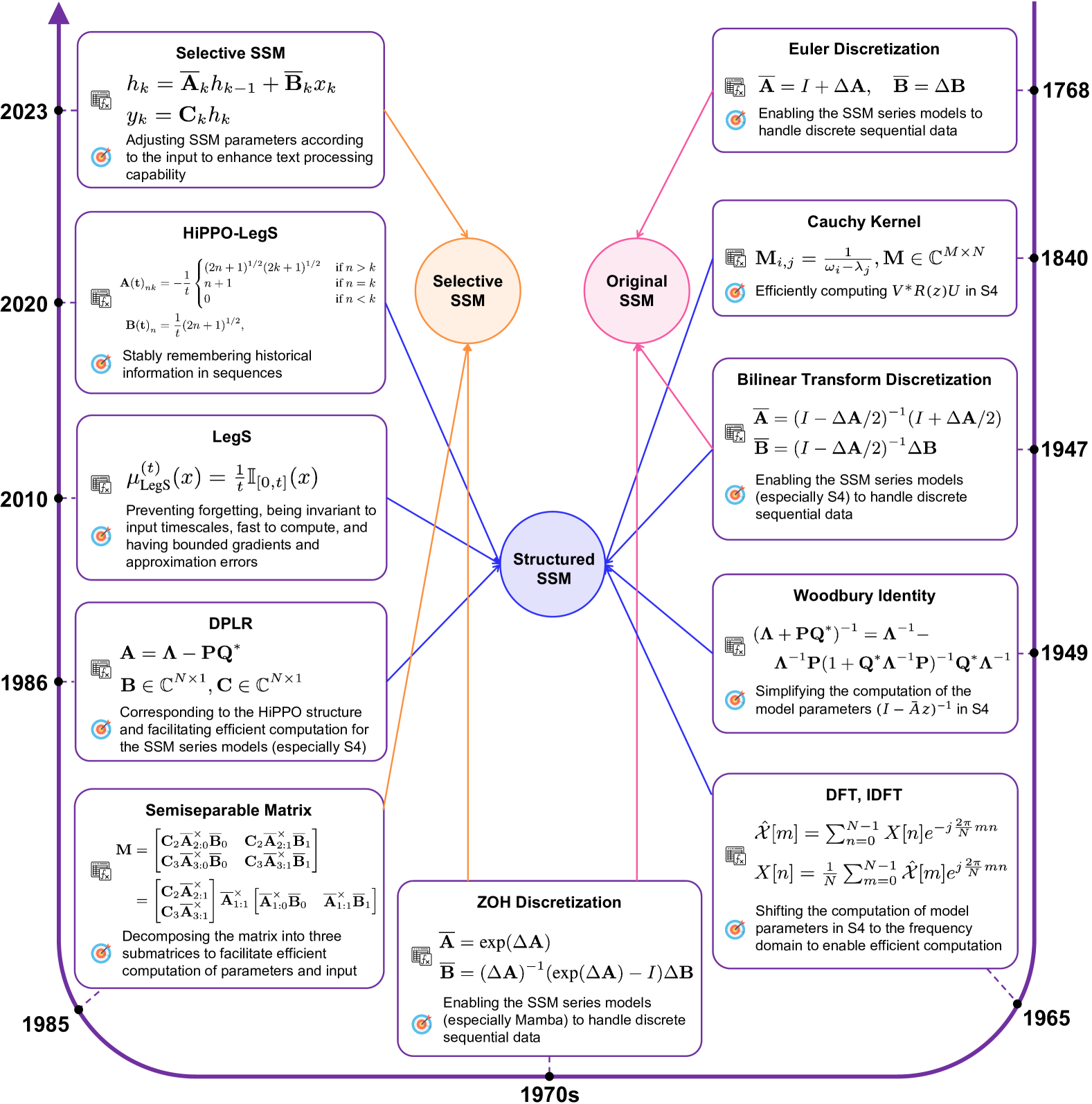
Figure 1: Technologies of SSM Series and their corresponding relationships. Each technical description card includes the technique’s name, mathematical formulation, and objective.

Several key techniques have provided technical support and ensured the development of the SSM series. Methods such as Euler’s method (euler1794institutiones), zero-order hold (ZOH), and bilinear transform (tustin1947method) discretization enable the transformation of SSMs from continuous-time to discrete-time, allowing these models to effectively handle discrete sequential data. To enhance the performance of SSMs, researchers have introduced mathematical techniques like LegS (hosny2010refined), HiPPO (gu2020hippo), and selective SSM (dao2024transformers). These techniques enable stable retention of historical sequence information and significantly improve the models’ text processing capabilities. In terms of efficiency, techniques such as DPLR (antoulas1986scalar), DFT, IDFT (cooley1969finite), semi-separable matrices (gohberg1985linear) lay the foundation for faster computations, and tools like the Woodbury identity (woodbury1949stability) and Cauchy kernel (cauchy1840exercices) streamline the computational processes. Together, these recent advancements greatly improve the computational efficiency of SSMs with little to no loss in performance. Figure 1 presents these techniques and their corresponding relationships with different models in chronological order.

In this survey, We first introduce the mathematical formulation of SSMs in Section 2. Next, Section 3 explores additional structures in SSMs with works such as S4, Section 4 introduces selectivity for SSMs leading with Mamba. These sections focus on detailing core techniques, summarizing optimization strategies in model architectures, and discussing theoretical analyses. Section LABEL:SSM_and_Other_Model_Architecture explores the relationship between SSMs and other model structures, particularly Transformer, and examines the trends in SSM architecture optimization. Section LABEL:Application highlights the applications of SSMs across various domains, including video processing, molecular modeling, speech and audio analysis, and so on.

for tree= forked edges, grow’=0, draw, rounded corners, node options=align=center,, text width=2.7cm, s sep=6pt, calign=child edge, calign child=(n_children()+1)/2, , [SSM Series, fill=gray!45, parent [Original SSM, for tree=fill=green!45, o_ssm [Architecture Variants, o_ssm [Deep SSM (NEURIPS2018_5cf68969); LOCOST (bronnec2024locost);2D-SSM (baron2024a);Spectral State Space Models (agarwal2024spectral);SpaceTime (zhang2023effectively);LMUFFT (10289082), o_ssm_work] ] [Application, o_ssm [Point2SSM (adams2024pointssm);NCDSSM (ansari2023neuralcontinuousdiscretestatespace),o_ssm_work] ] ] [Structured SSM, for tree=fill=red!45,s4 [Architecture Variants, s4 [S4 (gu2021efficiently); S4D (gu2022parameterizationinitializationdiagonalstate);S4ND (nguyen2022s4ndmodelingimagesvideos);DSS (gupta2022diagonalstatespaceseffective);S5 (smith2023simplifiedstatespacelayers);Liquid-S4 (hasani2022liquid);BiGS (wang2023pretraining);GSS (mehta2022long);SMA (ren2023sparse);BST (fathi2023block-state);SPADE (zuo2022efficient);
GateLoop (katsch2024gateloop);Decision S4 (bardavid2023decisions4efficientsequencebased);ConvS5 (smith2023convolutionalstatespacemodels), s4_work] ] [Appication, s4 [LS4 (zhou2023deeplatentstatespace);SaShiMi (goel2022itsrawaudiogeneration);TranS4mer (islam2023efficientmoviescenedetection);DSSformer (saon2023diagonalstatespaceaugmented);
S4M (chen2023neuralstatespacemodelapproach);ViS4mer (islam2023longmovieclipclassification);DiffuSSM (yan2023diffusionmodelsattention);Hieros (mattes2024hieroshierarchicalimaginationstructured);
R2I (samsami2024masteringmemorytasksworld);GraphS4mer (tang2023modelingmultivariatebiosignalsgraph);Graph-S4 (gazzar2022improvingdiagnosispsychiatricdisorders);fMRI-S4 (elgazzar2022fmris4learningshortlongrange);Spiking-S4 (du2024spikingstructuredstatespace), s4_work] ] ] [Selective SSM, for tree=fill=blue!45, mamba [Architecture Variants, mamba [General[Mamba (gu2023mamba); Jamba (lieber2024jamba);MambaMixer (behrouz2024mambamixer);
MoE-Mamba (Pioro2024MoEMambaES);BlackMamba (Anthony2024BlackMambaMO);
DenseMamba (He2024DenseMambaSS);Hierarchical SSM (Bhirangi2024HierarchicalSS);SIMBA (patro2024simbasimplifiedmambabasedarchitecture);Mamba4Rec (liu2024mamba4recefficientsequentialrecommendation);
MambaFormer (park2024mambalearnlearncomparative);ReMamba (yuan2024remambaequipmambaeffective);
Samba (ren2024sambasimplehybridstate),mamba_work] ] [Vision [Vision Mamba (zhu2024visionmambaefficientvisual);VMamba (liu2024vmambavisualstatespace);Graph-Mamba (wang2024graphmambalongrangegraphsequence);Mamba-ND (li2024mambandselectivestatespace);Gamba (shen2024gambamarrygaussiansplatting);Pan-Mamba (he2024panmambaeffectivepansharpeningstate);MambaIR (guo2024mambairsimplebaselineimage);VL-Mamba (qiao2024vlmambaexploringstatespace);SpikeMba (li2024spikembamultimodalspikingsaliency);
Video Mamba Suite (chen2024videomambasuitestate);
Zigma (hu2024zigmaditstylezigzagmamba);LocalMamba (huang2024localmambavisualstatespace);Plain-Mamba (yang2024plainmambaimprovingnonhierarchicalmamba),mamba_work] ] [Multi-Modal [Cobra (zhao2024cobraextendingmambamultimodal);Sigma (wan2024sigmasiamesemambanetwork);Fusion-Mamba (dong2024fusionmambacrossmodalityobjectdetection),mamba_work] ] ] [Application, mamba [Medical [ Mamba-UNet (wang2024mambaunetunetlikepurevisual);
Vivim (yang2024vivimvideovisionmamba);MambaMorph (guo2024mambamorphmambabasedframeworkmedical);
VM-UNet (ruan2024vmunetvisionmambaunet);Swin-UMamba (liu2024swinumambamambabasedunetimagenetbased);nnMamba (gong2024nnmamba3dbiomedicalimage);FD-Vision Mamba (zheng2024fdvisionmambaendoscopicexposure);Semi-Mamba-UNet (ma2024semimambaunetpixellevelcontrastivepixellevel);P-Mamba (ye2024pmambamarryingperonamalik);MamaMIR (huang2024mambamirarbitrarymaskedmambajoint);Weak-Mamba-UNet (wang2024weakmambaunetvisualmambamakes);CMT-MMH (zhang2024motionguideddualcameratrackerendoscope);Caduceus (schiff2024caduceusbidirectionalequivariantlongrange);MambaMIL (yang2024mambamilenhancinglongsequence);
CMViM (yang2024cmvimcontrastivemaskedvim);T-Mamba (hao2024tmambaunifiedframeworklongrange);
ProMamba (xie2024promambapromptmambapolypsegmentation), mamba_sub_work ]] [Point Cloud [3DMambaComplete (li20243dmambacompleteexploringstructuredstate);
PointMamba (liang2024pointmambasimplestatespace);Point Cloud Mamba (zhang2024pointcloudmambapoint),mamba_sub_work] ] [Others [U-Mamba (ma2024umambaenhancinglongrangedependency);SegMamba (xing2024segmambalongrangesequentialmodeling);Res-VMamba (chen2024resvmambafinegrainedfoodcategory);O-Mamba (dong2024omambaoshapestatespacemodel);
Motion Mamba (zhang2024motionmambaefficientlong);STG-Mamba (li2024stgmambaspatialtemporalgraphlearning);RS3Mamba (ma2024rs3mambavisualstatespace);
MambaTab (ahamed2024mambatab);MambaByte (Wang2024MambaByteTS);
MambaStock (shi2024mambastockselectivestatespace);HARMamba (li2024harmambaefficientlightweightwearable);
RhythmMamba (zou2024rhythmmambafastremotephysiological),mamba_sub_work] ] ] ] ]

Figure 2: Typology of SSM Series. The “Architecture Variants” presents the common SSM architectures, while the “Application” shows the practical implementations of SSMs in real-world scenarios.

2 State Space Models: From Continuous To Discrete

The concept of state space, along with the state space model, holds a significant historical backdrop. The continuous-time state space model is a pivotal and versatile tool for describing dynamical systems. Early applications of state space models include theoretical physics, communication signal processing, system control, and allied fields (findlay1904phase; bubnicki2005modern). Notably, Kalman (kalman1960new) employs state space models to characterize linear dynamic systems and resolve the optimal estimation problem. By directly discretizing the continuous-time SSM, we obtain the discrete-time SSM, also referred to as the original SSM in this survey. The discrete-time SSM is capable of handling a series of discrete input data and has been increasingly gaining attention as a sequence model.

In this chapter, Section 2.1 introduces the continuous-time State Space Model. Section 2.2 presents the discretization methods and the resulting discrete-time SSM. Section 2.3 discusses several fundamental properties of SSMs, while Section 2.4 explores some model structures with the original SSM.

2.1 Continuous-Time State Space Models

The classical linear continuous-time state space model (SSM) was first widely employed in control system theory (kalman1960new). It describes dynamical systems through specific differential equations, and can be expressed as the following:

$$h^{\prime}(t)=\mathbf{A}(t)h(t)+\mathbf{B}(t)x(t),$$ (1)

$$y(t)=\mathbf{C}(t)h(t)+\mathbf{D}(t)x(t),$$ (2)

where $x(t)\in\mathbb{R}^{N_{\text{in}}}$ is the input vector signal, $h(t)\in\mathbb{R}^{N_{\text{s}}}$ is the hidden state vector signal, and $y(t)\in\mathbb{R}^{N_{\text{out}}}$ is the output vector signal. The matrices $\mathbf{A}(t)$, $\mathbf{B}(t)$, $\mathbf{C}(t)$, and $\mathbf{D}(t)$ represent the parameter matrices of the state space model. Specifically, $\mathbf{A}(t)\in\mathbb{R}^{N_{\text{s}}\times N_{\text{s}}}$ is the system matrix, which describes how the current state influences its rate of change. $\mathbf{B}(t)\in\mathbb{R}^{N_{\text{s}}\times N_{\text{in}}}$, the control matrix, represents the effect of the input on the state change. $\mathbf{C}(t)\in\mathbb{R}^{N_{\text{out}}\times N_{\text{s}}}$, the output matrix, captures how the system states affect the output. $\mathbf{D}(t)\in\mathbb{R}^{N_{\text{out}}\times N_{\text{in}}}$, the feed-forward matrix, illustrates direct input-output relationships, circumventing system states. Generally, in control systems or real-world physical systems, these parameters are either determined by the inherent characteristics of the system or acquired through conventional statistical inference methods.

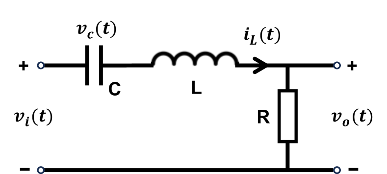
Figure 3: The illustration of a RC oscillator circuit, where $L$, $C$, and $R$ denote the inductance, capacitance and resistance, respectively.

The classical continuous-time SSM can capture many systems in a wide range of subjects. For instance, it can model the RC oscillator circuit system shown in Figure 3, where $v$, $i$, $L$, $C$, and $R$ represent the voltage, current, inductance, capacitance and resistance, respectively. Let the input signal be the system’s input voltage $[v_{i}(t)]=x(t)$, the output signal be the system’s output voltage $[v_{o}(t)]=y(t)$, and the two components of the system’s hidden state be the current in the inductor and the voltage across the capacitor $[i_{L}(t),v_{c}(t)]^{T}=h(t)$. Derived from fundamental physical principles such as Ohm’s law and Kirchhoff’s circuit laws, the state space model for this system can be expressed as:

$$h^{\prime}(t)=\mathbf{A}(t)h(t)+\mathbf{B}(t)x(t)=\bigg{[}\begin{matrix}-R&0\\ 0&-1\end{matrix}\bigg{]}h(t)+[1]x(t),$$ (3)

$$y(t)=\mathbf{C}(t)h(t)+\mathbf{D}(t)x(t)=\bigg{[}\begin{matrix}-L\nabla_{t}&0\\ 0&-1\end{matrix}\bigg{]}h(t)+[1]x(t).$$ (4)

SSM effectively describes how systems evolve over time. Much like tracking a moving object, the model uses its current position (state) to predict where it will go next. Since every change in the system follows clear mathematical rules, it is possible to predict future behavior or estimate hidden information from partial observations. Furthermore, SSM is particularly suitable for describing complex systems, as it can simultaneously handle multiple inputs and outputs. For example, when tracking a rocket, inputs might include factors like fuel and wind speed, states could represent position and velocity, and outputs could correspond to the measurements recorded by the sensors.

2.2 Discretization of Continuous-Time SSMs

The above SSM described by Eq. 1,2 is termed the continuous-time SSM because $x(t)$, $h(t)$, and $y(t)$ represent continuous-time signals. However, in most practical applications, the model inputs, hidden states, and outputs are instead discrete sequences, denoted as $x=(x_{0},x_{1},x_{2},\dots)$, $h=(h_{0},h_{1},h_{2},\dots)$, $y=(y_{0},y_{1},y_{2},\dots)$. For instance, when processing natural language, the input and output of the model are token embeddings, which are discrete values rather than continuous functions. Directly applying the continuous-time SSM to discrete data requires fitting the discrete data points into continuous signals, a complex and rarely used process. Instead, a more effective and practical approach is to discretize the SSM.

Essentially, the discrete-time SSM parameters $\overline{\mathbf{A}}$ and $\overline{\mathbf{B}}$ are expressed in terms of the continuous-time SSM parameters $\mathbf{A}$, $\mathbf{B}$, and an additional time-step parameter $\Delta$. And the discretization of SSMs generally involves addressing the ordinary differential equation (ODE) within the model representation. The discrete-time SSM can be represented by the following difference equations:

$$h_{k}=\overline{\mathbf{A}}h_{k-1}+\overline{\mathbf{B}}x_{k},$$ (5)

$$y_{k}=\mathbf{C}h_{k}+\mathbf{D}x_{k},$$ (6)

where $x_{k}\in\mathbb{R}^{N_{\text{in}}}$, $h_{k}\in\mathbb{R}^{N_{\text{s}}}$ and $y_{k}\in\mathbb{R}^{N_{\text{out}}}$ denote one single data point of the input, hidden state, and output data sequences respectively. $\overline{\mathbf{A}}\in\mathbb{R}^{N_{\text{s}}\times N_{\text{s}}}$, $\overline{\mathbf{B}}\in\mathbb{R}^{N_{\text{s}}\times N_{\text{in}}}$, $\mathbf{C}\in\mathbb{R}^{N_{\text{out}}\times N_{\text{s}}}$, and $\mathbf{D}\in\mathbb{R}^{N_{\text{out}}\times N_{\text{in}}}$ are model parameters of the discrete-time SSM.

Notably, the parameter matrix $\mathbf{D}$, when researched as a sequence model, is often disregarded. This is because $\mathbf{D}$ is generally viewed as a skip connection and does not directly influence the state $h$. Usually, $\mathbf{D}$ is easy to compute, and can be approximated by other structures. Consequently, Eq. 5,6 are commonly expressed as

$$h_{k}=\overline{\mathbf{A}}h_{k-1}+\overline{\mathbf{B}}x_{k},$$ (7)

$$y_{k}=\mathbf{C}h_{k}$$ (8)

Common discretization methods include Euler’s method (euler1794institutiones), zero-order hold (ZOH), and the bilinear transform (gu2023modeling):

$$\textbf{(Euler)}\quad\quad\overline{\mathbf{A}}=I+\Delta\mathbf{A},\quad\quad\overline{\mathbf{B}}=\Delta\mathbf{B},$$ (9)

$$\textbf{(ZOH)}\quad\quad\overline{\mathbf{A}}=\text{exp}(\Delta\mathbf{A}),\quad\quad\overline{\mathbf{B}}=(\Delta\mathbf{A})^{-1}(\text{exp}(\Delta\mathbf{A})-I)\Delta\mathbf{B},$$ (10)

$$\textbf{(Bilinear)}\quad\overline{\mathbf{A}}=(I-\Delta\mathbf{A}/2)^{-1}(I+\Delta\mathbf{A}/2),\quad\quad\overline{\mathbf{B}}=(I-\Delta\mathbf{A}/2)^{-1}\Delta\mathbf{B}.$$ (11)

The discrete-time SSM can be used as a sequence model to model and process data that can be serialized. For example, in natural language processing, given an input sequence $x=(x_{0},x_{1},x_{2},\dots)$ where each $x_{i}$ represents the embedding vector of a linguistic token, the SSM can iteratively apply Eq. 7,8 to compute the hidden state-output pairs $(h_{0},y_{0}),(h_{1},y_{1}),\dots$ This recurrent computation process ultimately generates the output token representations $y=(y_{0},y_{1},y_{2},\dots)$. When both the input token embeddings and the corresponding desired output token representations are provided, the SSM can be trained to model the relationship between them. This establishes its capability for modeling sequential linguistic information. In this paper, we focus on SSMs as sequence models and use "SSM" to refer to the discrete-time SSM unless otherwise specified.

2.3 Fundamental Properties of SSMs

The discrete-time SSM described by Eq. 7,8 can handle discrete sequential data and serve as a sequence model. We next discuss some fundamental properties of SSMs in this context.

A crucial property of the discrete-time SSM is its linearity. Specifically, when emphasizing the input and output and simplifying Eq. 7,8 to $y=\text{SSM}(\overline{\mathbf{A}},\overline{\mathbf{B}},\mathbf{C})(x)$, it follows that

$$\text{SSM}(\overline{\mathbf{A}},\overline{\mathbf{B}},\mathbf{C})(x^{1}+x^{2})=\text{SSM}(\overline{\mathbf{A}},\overline{\mathbf{B}},\mathbf{C})(x^{1})+\text{SSM}(\overline{\mathbf{A}},\overline{\mathbf{B}},\mathbf{C})(x^{2}),$$ (12)

where $x^{1}=(x^{1}_{0},x^{1}_{1},x^{1}_{2},\dots)$, $x^{2}=(x^{2}_{0},x^{2}_{1},x^{2}_{2},\dots)$ represent two different sets of input data. Another characteristic of linearity is that the model parameters $\overline{\mathbf{A}},\overline{\mathbf{B}},\mathbf{C}$ are independent of the input data $x$. On one hand, this linearity enables optimizations for computational efficiency and parallelization, which will be discussed in Chapter 3. On the other hand, linear models often struggle with fitting complex data. Chapter 4 will provide a detailed discussion of enabling input-dependent parameterization of model parameters $\overline{\mathbf{A}},\overline{\mathbf{B}},\mathbf{C}$, thereby transforming the SSM into a nonlinear architecture with enhanced selectivity.

Another fundamental property of SSM is that its expression can be derived into various forms. For instance, Eq. 7,8 naturally align with the representation format of recurrent models. These expressions can also lead to the derivation of convolutional forms, such that:

$$y=x*\overline{{\mathbf{K}}}\quad where\quad x=(x_{0},x_{1},x_{2},\dots),\overline{\mathbf{K}}=(\mathbf{C}\overline{\mathbf{B}},\mathbf{C}\overline{\mathbf{AB}},\mathbf{C}\overline{\mathbf{A}}^{2}\overline{\mathbf{B}},\dots).$$ (13)

This convolutional structure creates the conditions necessary for the efficient computational algorithms introduced in Chapter 3. This diversity of SSM expressions opens up flexibility in architectural modifications.

Furthermore, the SSM has several inherent limitations, including non-parallelizable computations, instability in capturing long sequence dependencies, and constrained approximation capacity. These challenges can be addressed by incorporating structured parameters and selectivity, as will be elaborated in Chapters 3 and 4. In this paper, we refer to the SSM described by Eq. 7,8 as the "original SSM" or the "vanilla SSM".

2.4 Models with Original SSMs

Despite its limitations, the original SSM remains widely used in some studies, including recent works, due to its simplicity and ease of implementation. This section presents some models that incorporate the original SSM. These model structures either embed the original discrete SSM within other architectures or integrate new computational modules into the SSM structure. These modifications improve performance on tasks such as time series forecasting, long-text summarization, and two-dimensional data processing.

To accomplish long document abstractive summarization, Bronnec et al. (bronnec2024locost) construct an encoder layer with an SSM as its central component, termed the LOCOST. Starting from the convolutional representation of SSM, they introduce the Bidirectional SSM, which incorporates causal convolution and cross-correlation to simultaneously consider contextual information before and after each token in the sequence. This architecture builds upon the low computational complexity and superior long sequence handling of SSMs and further achieves improved context capture. Baron et al. (baron20232) propose a 2-D SSM layer based on Roesser’s SSM model (givone1972multidimensional). It expands states to capture both horizontal and vertical information, enhancing the SSM’s understanding of two-dimensional data. Agarwal et al. (agarwal2024spectral) apply the Spectral Filtering algorithm to learn linear dynamical systems. The proposed Spectral SSM employs fixed spectral filters that obviate the need for learning. It therefore effectively maps input sequences to a new representation space and captures long-term dependencies in sequential data. These features improve the model’s prediction performance and stability, especially in sequences containing long-range dependencies. Zhang et al. (zhang2023effectively) introduce a closed-loop prediction mechanism to SSMs, where the SSM at the decoder layer not only receives information from the encoder layer but also incorporates feedback from its own output. This design improves the model’s flexibility and accuracy in handling long-term prediction tasks.

3 Structured State Space Models

The introduction of structured parameters to SSMs is considered to be one of the most remarkable recent advancements for sequence modeling. By the application of various structures to the parameters in SSMs, the effectiveness and efficiency of these models are improved. As one of the most prominent structured SSMs, S4 has garnered widespread attention and influence (gu2021efficiently). Within this chapter, we first discuss the structures of model parameters introduced by S4 with an emphasis on its theoretical motivations. Next, we consider other structural mechanisms beyond S4. Lastly, we explore the role SSMs play as a part of more sophisticated models. Section 3.1 provides an overview of the structured SSM, especially S4, from an accessible perspective without delving into details. Sections 3.2, 3.3 elaborate on S4 from a theoretical perspective, focusing on its effectiveness and efficiency, respectively. Section 3.4 summarizes alternative structures to which the parameters of SSMs are restricted. Section 3.5 reviews models that integrate structured SSM as a core component.

3.1 Overview of Structured State Space Models

The term structured SSM refers to SSMs where specific structures have been applied to their system dynamics. The exact structures can be formulated by a number of sophisticated methods such as initialization, parameterization or placing explicit constraints on parameters. For example, consider a model parameter matrix $\mathbf{W}\in\mathbb{R}^{N\times N}$. When its off-diagonal elements are restricted to zero, $\mathbf{W}$ becomes a diagonal matrix and thus qualifies as a structured parameter. This diagonal structure reduces storage overhead and computational cost. In contrast to original unconstrained SSMs, structured SSMs such as S4 exhibit a number of desirable mathematical properties, which greatly enhance their effectiveness and efficiency.

Specifically, S4 demonstrated exceptional performance across a wide range of sequence modeling tasks. This is achieved by introducing a series of structural features: S4 first leverages HiPPO (gu2020hippo) to constrain parameters to the Legendre memory unit (discussed in detail in Section 3.2). This specific structure enables S4 to address challenges associated with memory retention for long-range dependencies and alleviate issues such as gradient vanishing. Additionally, S4 employs the Diagonal Plus Low-Rank (DPLR) (antoulas1986scalar) structure (elaborated in Section 3.3), which facilitates the use of efficient algorithms. These algorithms enable parallel training and boost computational efficiency and stability. With the introduction of DPLR, the computational complexity is reduced from $O(LN_{\text{s}}^{2})$ to $O(L+N)$. Beyond S4, alternative structured SSM variants employ different structural constraints. These modifications seek to refine and simplify the structured SSM framework and address the various inherent challenges in SSMs, including exponential memory decay, gradient vanishing, gradient explosion, instability in capturing long sequence dependencies, low training efficiency, and limited parallel computing capabilities.

3.2 Effectiveness: High-Order Polynomial Projection Operators (HiPPO)

The traditional discrete-time SSM framework suffers from suboptimal performance, with issues such as exponential memory decay and instability in capturing long sequence dependencies. These issues stem from the model’s inability to effectively retain the input history. S4 seeks to address these issues by utilizing structured parameters, the specific structure of which is derived through the HiPPO framework (gu2020hippo).

Conceptually speaking, HiPPO addresses the following core problem: How to efficiently reconstruct the history of input $x$ using state $h$? This problem can be formulated precisely as an online function approximation problem, which is investigated in HiPPO. In this subsection, we provide a detailed exposition of the HiPPO framework, discuss its specific instances and advantages, and explore the relationship between HiPPO and S4.

Gu et al. (gu2020hippo) specifically define memory through the online function approximation problem, which involves representing a function by storing coefficients of a set of basis functions. Mathematically, given a function $f(t)\in\mathbb{R}$ on $t\geq 0$ and a probability measure $\mu$, the distance between two functions $f$ and $g$ can be expressed as $\left\langle f,g\right\rangle_{\mu}=\int_{0}^{\infty}f(x)g(x)d\mu(x)$, and the norm of function $f$ can be defined as $\left\|f\right\|_{L_{2}(\mu)}=\left\langle f,f\right\rangle_{\mu}^{1/2}$. Moreover, the cumulative history is typically represented as $f_{\leq t}:=f(s)|_{s\leq t}$.  Solving the online approximation problem in this setup involves seeking $g^{(t)}\in\mathcal{G}$, typically a subspace spanned by orthogonal bases, that minimizes $\|f_{\leq t}-g^{(t)}\|_{L_{2}(\mu^{(t)})}$. The HiPPO framework aims to optimize this approximation at every timestep t.

Specifically, given an input function $f(t):\mathbb{R}^{+}\rightarrow\mathbb{R}$ on $t\geq 0$ and a time-varying measure family $\mu^{(t)}$, the HiPPO framework consists of the following three steps:

1. Obtain the Set of Bases.  The first step in HiPPO is to generate a suitable set of basis functions $\{g_{n}^{(t)}\}_{n\in\{0,1,\dots,N-1\}}$ according to $\mu^{(t)}$. $\{g_{n}^{(t)}\}$ should satisfy $\langle g_{n}^{(t)},g_{m}^{(t)}\rangle_{\mu^{(t)}}=\lambda_{n}^{2}\delta_{n,m}$, where $\delta$ is the impulse function. $\lambda_{n}$ is typically set to $\pm 1$ to ensure $\{g_{n}^{(t)}\}$ forms the orthogonal bases. This set of bases spans an N-dimensional subspace $\mathcal{G}$.

2. Calculate the Optimal Coefficients.  Given the generated basis set $\{g_{n}^{(t)}\}$, the next step is finding the optimal representation of input signal $f_{\leq t}:=f(s)|_{s\leq t}$ in the form of a polynomial $g^{(t)}={\sum_{n=0}^{N-1}}c_{n}(t)g_{n}^{(t)}$. Here, $c_{n}(t)$ denotes the optimal coefficients to construct polynomial $g^{(t)}=\text{argmin}_{g\in\mathcal{G}}\|f_{\leq t}-g\|_{\mu^{(t)}}$. With the orthogonality of the bases, the optimal coefficients can be computed through the following,

   $$c_{n}(t)=\left\langle f_{\leq t},g_{n}^{(t)}\right\rangle_{\mu^{(t)}}.$$ (14)

   The HiPPO paper denotes the results of the calculations, $g^{(t)}$ and $c(t):=(c_{n}(t))_{0\leq n<N}$ as $\text{proj}_{t}$ and $\text{coef}_{t}$, respectively.

3. Differentiate Equation 14 and Yield the ODE.  The last equation shows how to calculate $c(t)$ given a signal $f(t)$. However, in a continuous-time state space system, $c(t)$ denotes the state and $f(t)$ denotes the input which changes over time. In order to establish a closer connection with the expression of SSM (Equation 1), it is necessary to find the optimal matrices $\mathbf{A}$ and $\mathbf{B}$, Furthermore, $\mathbf{A}$ and $\mathbf{B}$ should remain independent of $f(t)$. This can be achieved by taking the derivative of the previous equation. Given the Equation 14, the differentiation of state $c(t)$ is calculated with respect to the input function $f(t)$. This is depicted by the following ordinary differential equation (ODE):

   $$\frac{d}{dt}c(t)=\mathbf{A}(t)c(t)+\mathbf{B}(t)f(t),$$ (15)

   where $\mathbf{A}(t)\in\mathbb{R}^{N\times N}$ and $\mathbf{B}(t)\in\mathbb{R}^{N\times 1}$ often remain independent of $f(t)$ and are solely related to the measure $\mu^{(t)}$ and the orthogonal subspace $\mathcal{G}$. Equation 15 offers a general strategy for computing coefficients $c(t)$.

In essence, HiPPO can be conceptualized as a system: given a function $f(t)$ and a measure $\mu^{(t)}$, it outputs the optimal representation coefficients $c(t)$ of $f(t)$ under $\mu^{(t)}$. It is worth noting that, in most cases, researchers are primarily interested in the dynamic relationships between $f(t)$ and $c(t)$, which are represented by $\mathbf{A}(t)$ and $\mathbf{B}(t)$. Hence, HiPPO can also be viewed as a black box: given a measure $\mu^{(t)}$, it outputs the corresponding structured parameter matrices $\mathbf{A}(t)$ and $\mathbf{B}(t)$ satisfying the OED Equation 15 and yielding the optimal representation coefficients $c(t)$.

Given specific measure, the HiPPO framework is able to generate optimal state-space equations. We discuss two notable SSM-related HiPPO instances, LegT and LegS. The first variant entails the use of the translated Legendre (LegT) measures. LegT can be expressed as $\mu^{(t)}_{\text{LegT}}(x)=\frac{1}{\theta}\mathbb{I}_{\left[t-\theta,t\right]}(x)$, where $\theta$ denotes the length of the history being memorized. This measure assigns uniform weights to nearby histories. Through the HiPPO framework, the structured parameter matrices $\mathbf{A}$ and $\mathbf{B}$ corresponding to LegT can be determined as

$$\mathbf{A}_{nk}=-\frac{1}{\theta}\begin{cases}(-1)^{n-k}(2n+1)&\text{ if }n\geq k\\ 2n+1&\text{ if }n\leq k\end{cases},\quad\mathbf{B}_{n}=\frac{1}{\theta}(2n+1)(-1)^{n},$$ (16)

which is exactly the parameter matrices of the Legendre Memory Unit (LMU) (voelker2019legendre), an improved model of RNN.

The second example comprises the scaled Legendre (LegS) measures (hosny2010refined), denoted as $\mu^{(t)}_{\text{LegS}}(x)=\frac{1}{t}\mathbb{I}_{\left[0,t\right]}(x)$, for which the corresponding structured parameter matrices $\mathbf{A}$ and $\mathbf{B}$ satisfy:

$$t\mathbf{A}(t)_{nk}=-\begin{cases}(2n+1)^{1/2}(2k+1)^{1/2}&\text{ if }n>k\\ n+1&\text{ if }n=k\\ 0&\text{ if }n<k\end{cases},\quad t\mathbf{B}(t)_{n}=(2n+1)^{1/2},$$ (17)

obtained through the HiPPO framework. LegS is an optimization over LegT. It scales the window over time and assigns uniform weights to all history. Advantages of LegS include mitigation of forgetting, invariance to input timescale, faster computations, and bounded gradients and approximation errors.

The HiPPO framework outputs the structured parameter matrices $\mathbf{A}(t)$ and $\mathbf{B}(t)$ that satisfy Equation 15 and yield the optimal coefficients $c(t)$ for representing $f(t)$. In other words, setting the same $\mathbf{A}(t)$ and $\mathbf{B}(t)$ or similar parameter matrices in Equation 1 enables the state $h(t)$ to optimally represent the input $x(t)$, thereby achieving the memorization of history.

S4 utilizes the specific structures generated by HiPPO to help with its long-range dependencies. Although the matrices in Equation 17 are optimal in theory, empirical results have shown that making parameters $\mathbf{A}(t)$ and $\mathbf{B}(t)$ trainable can further improves performance in general. In S4, if the parameters $\mathbf{A}$ and $\mathbf{B}$ are not trained, they are restricted to specific structures through HiPPO. However, training the parameters generally yields better results, hence HiPPO is commonly used for initialization. Typically, initialization often involves using the $t\mathbf{A}(t)$ and $t\mathbf{B}(t)$ corresponding to the LegS (i.e. Equation 17) and discretizing through Equation 11 in S4.

3.3 Efficiency: Diagonal Plus Low-Rank

Another crucial challenge addressed by S4 is computational efficiency. The complexity of the calculating the original SSM in Eq. 7,8 is $O(LN^{2})$. And its training process lacks parallelizability. S4 overcomes this limitation by introducing of a special structure named Diagonal Plus Low-Rank (DPLR) (antoulas1986scalar) and employing a series of algorithms designed for parallel training and efficient computation.

The SSM with DPLR structure satisfies $\mathbf{A}=\mathbf{\Lambda}-\mathbf{P}\mathbf{Q}^{*},\mathbf{B}\in\mathbb{C}^{N\times 1},\mathbf{C}\in\mathbb{C}^{1\times N}$, where $\mathbf{\Lambda}\in\mathbb{C}^{N\times N}$ is diagonal and $\mathbf{P},\mathbf{Q}\in\mathbb{C}^{N\times 1}$ is low-rank. The corresponding algorithm begins with the convolutional representation of SSM: by recursively applying Equation 5,8, $y_{k}=\mathbf{C}\overline{\mathbf{A}}^{k}\overline{\mathbf{B}}x_{0}+\mathbf{C}\overline{\mathbf{A}}^{k-1}\overline{\mathbf{B}}x_{1}+\dots+\mathbf{C}\overline{\mathbf{AB}}x_{k-1}+\mathbf{C}\overline{\mathbf{B}}x_{k}$ can be derived This equation leads to

$$y=\overline{\mathbf{K}}*x,\quad\overline{\mathbf{K}}\in\mathbb{R}^{L}:=(\mathbf{C}\overline{\mathbf{A}}^{n}\overline{\mathbf{B}})_{n\in[L]}=(\mathbf{C}\overline{\mathbf{B}},\mathbf{C}\overline{\mathbf{AB}},\dots,\mathbf{C}\overline{\mathbf{A}}^{L-1}\overline{\mathbf{B}})$$ (18)

where $x=(x_{0},x_{1},\dots,x_{L-1})$ is an input of length L. In Equation 18, the complexity of computing $\overline{\mathbf{K}}$ is $O(LN^{2})$, making the efficient computation of $\overline{\mathbf{K}}$ a central aspect of the algorithm.

The first pivotal step of this algorithm involves shifting the computation of $\overline{\mathbf{K}}$ to the frequency domain by computing its Discrete Fourier Transform (DFT) (cooley1969finite). This can be denoted as

$$\hat{\mathcal{K}}_{L}(z;\overline{\mathbf{A}},\overline{\mathbf{B}},\mathbf{C})\in\mathbb{C}:=\sum_{n=0}^{L-1}\bar{\mathbf{C}}\overline{\mathbf{A}}^{n}\overline{\mathbf{B}}z^{n}=\bar{\mathbf{C}}(\mathbf{I}-\overline{\mathbf{A}}^{L}z^{L})(\mathbf{I}-\overline{\mathbf{A}}z)^{-1}\overline{\mathbf{B}}=\tilde{\mathbf{C}}(\mathbf{I}-\overline{\mathbf{A}}z)^{-1}\overline{\mathbf{B}},$$ (19)

where $\bar{\mathbf{C}}$ denotes the conjugate of $\mathbf{C}$, $z\in\Omega=\left\{\text{exp}(-2\pi i\frac{k}{L}):k\in[L]\right\}$, $\tilde{\mathbf{C}}=\bar{\mathbf{C}}(\mathbf{I}-\overline{\mathbf{A}}^{L}z^{L})=\bar{\mathbf{C}}(\mathbf{I}-\overline{\mathbf{A}}^{L})$. After obtaining the DFT, $\overline{\mathbf{K}}$ can be computed using the Fast Fourier Transform (FFT) algorithm, requiring $O(L\text{log}L)$ operations. It’s worth noting that in S4, $\tilde{\mathbf{C}}$ is directly learned via parameterization, obviating the need for computing $\tilde{\mathbf{C}}=\bar{\mathbf{C}}(\mathbf{I}-\overline{\mathbf{A}}^{L})$. This step replaces matrix power operations with efficient low-rank matrix inversions, presented as the subsequent step.

The second integral step of this algorithm simplifies the computation of $(\mathbf{I}-\overline{\mathbf{A}}z)^{-1}$ through using the Woodbury identity (woodbury1949stability). In the low-rank scenario, the Woodbury identity is

$$(\mathbf{\Lambda}+\mathbf{PQ}^{*})^{-1}=\mathbf{\Lambda}^{-1}-\mathbf{\Lambda}^{-1}\mathbf{P}(1+\mathbf{Q}^{*}\mathbf{\Lambda}^{-1}\mathbf{P})^{-1}\mathbf{Q}^{*}\mathbf{\Lambda}^{-1},$$ (20)

where $\mathbf{\Lambda}\in\mathbb{C}^{N\times N}$ is diagonal, $\mathbf{P},\mathbf{Q}\in\mathbb{C}^{N\times 1}$, and $(\mathbf{\Lambda}+\mathbf{PQ}^{*})^{-1}$ is invertible. Applying Equation 11,

$$\hat{\mathcal{K}}_{L}(z;\overline{\mathbf{A}},\overline{\mathbf{B}},\mathbf{C})=\tilde{\mathbf{C}}(\mathbf{I}-\overline{\mathbf{A}}z)^{-1}\overline{\mathbf{B}}=\frac{2}{1+z}\tilde{\mathbf{C}}\left(\frac{2}{\Delta}\frac{1-z}{1+z}-\mathbf{A}\right)^{-1}\mathbf{B}$$ (21)

can be derived. By leveraging the Woodbury identity and $\mathbf{A}=\mathbf{\Lambda}-\mathbf{P}\mathbf{Q}^{*}$ in the DPLR structure,

$$\hat{\mathcal{K}}_{L}(z;\overline{\mathbf{A}},\overline{\mathbf{B}},\mathbf{C}) =\frac{2}{1+z}\tilde{\mathbf{C}}\left(\frac{2}{\Delta}\frac{1-z}{1+z}-\mathbf{\Lambda}+\mathbf{P}\mathbf{Q}^{*}\right)^{-1}\mathbf{B}$$ (22)

$$=\frac{2}{1+z}\left[\tilde{\mathbf{C}}\mathbf{R}(z)\mathbf{B}-\tilde{\mathbf{C}}\mathbf{R}(z)\mathbf{P}(1+\mathbf{Q}^{*}\mathbf{R}(z)\mathbf{P})^{-1}\mathbf{Q}^{*}\mathbf{R}(z)\mathbf{B}\right],$$

where $\mathbf{R}(z)=\left(\frac{2}{\Delta}\frac{1-z}{1+z}-\mathbf{\Lambda}\right)^{-1}$. This step transforms the computation of $(\mathbf{I}-\overline{\mathbf{A}}z)^{-1}$ into the inversion of the diagonal matrix, streamlining the calculation process.

The final step of this algorithm focuses on efficiently computing $\mathbf{V}^{*}\mathbf{R}(z)\mathbf{U}$ using the Cauchy kernel (cauchy1840exercices). Leveraging the previous steps, the computation of $\overline{\mathbf{K}}$ is transformed into calculating four expressions in the format of $\mathbf{V}^{*}\mathbf{R}(z)\mathbf{U}$ (i.e. $\tilde{\mathbf{C}}\mathbf{R}(z)\mathbf{B}$, $\tilde{\mathbf{C}}\mathbf{R}(z)\mathbf{P}$, $\mathbf{Q}^{*}\mathbf{R}(z)\mathbf{P}$, $\mathbf{Q}^{*}\mathbf{R}(z)\mathbf{B}$). Given $\mathbf{V}^{*}\mathbf{R}(z)\mathbf{U}={\textstyle\sum_{n}}\frac{v_{n}^{*}u_{n}}{z-\lambda_{n}}$, computing $\mathbf{V}^{*}\mathbf{R}(z)\mathbf{U}$ for all $z\in\Omega=\left\{\text{exp}(-2\pi i\frac{k}{L}):k\in[L]\right\}$ entails a Cauchy matrix-vector multiplication. This process has been extensively researched and requires only $\tilde{O}(L+N)$ operations.

S4 constrains the parameter matrices to adhere to the DPLR structure. However, the limited expressivity of DPLR does not compromise the effectiveness of models such as S4 since techniques such as the HiPPO framework inherently satisfy this structure. Specifically, the HiPPO matrices adhere to the Normal Plus Low-Rank (NPLR) structure: $\mathbf{A}=\mathbf{V}\mathbf{\Lambda}\mathbf{V}^{*}-\mathbf{P}\mathbf{Q}^{*}=\mathbf{V}(\mathbf{\Lambda}-(\mathbf{V}^{*}\mathbf{P})(\mathbf{V}^{*}\mathbf{Q})^{*})\mathbf{V}^{*}$, where $\mathbf{V}\in\mathbb{C}^{N\times N}$ is unitary, $\mathbf{\Lambda}$ is diagonal, and $\mathbf{P},\mathbf{Q}\in\mathbb{R}^{N\times r}$. Particularly, the HiPPO matrices corresponding to LegS satisfy $r=1$. In this scenario, the NPLR structure is unitarily equivalent to DPLR.

In summary, S4 introduces the DPLR structure, shifts computations from time to frequency domain using the SSM’s convolutional expression, and simplifies calculations through the Woodbury identity and Cauchy kernel. It achieves parallel computation and reduces training complexity to $O(N(\tilde{N}+\tilde{L}))$.

3.4 Additional Structural Constraints for Structured SSMs

Sections 3.2 and 3.3 introduce two types of structured parameters in S4: the LegS structure derived from the HiPPO framework and the DPLR structure. In addition to these two types of structural constraints on model parameters, several other structural constraints have been proposed for structured SSMs. In this section, we examine additional structured parameters and their corresponding Structured SSMs, specifically S4D (gu2022parameterizationinitializationdiagonalstate) and DSS (gupta2022diagonalstatespaceseffective). A comparative analysis of these two structured SSMs is also presented.

The Diagonal State Space (DSS) (gupta2022diagonalstatespaceseffective) removes the low-rank component of the DPLR structure, retaining only the diagonalizable term $\mathbf{\Lambda}$. Compared to S4, DSS further reduces computational complexity with no significant loss of performance. Empirically, it achieves an average accuracy of 81.88 across six tasks in the Long Range Arena (LRA) benchmark (tay2020long), closely rivaling the 80.21 of S4. Its kernel from Eq. 13 can be derived and denoted as:

$$\mathbf{K} =\bar{\mathbf{K}}_{\mathbf{\Delta},L}\left(\mathbf{\Lambda},(1)_{1\leqslant i\leqslant N},\widetilde{w}\right)=\widetilde{w}\cdot\mathbf{\Lambda}^{-1}\left(e^{\mathbf{\Lambda}\mathbf{\Delta}}-I\right)\cdot\text{elementwise-exp}(\mathbf{P}),$$ (23)

where $\mathbf{K}\in\mathbb{R}^{1\times L}$ represents the kernel of length $L$ with a sampling interval $\mathbf{\Delta}>0$. $\widetilde{w}\in\mathbb{C}^{1\times N}$ is the parameter matrix. Matrix $\mathbf{P}\in\mathbb{C}^{N\times L}$ is defined as $\mathbf{P}_{i,k}=\lambda_{i}k\mathbf{\Delta}$. $\mathbf{\Lambda}$ is the diagonal matrix consisting of $\lambda_{1},\ldots,\lambda_{N}$, with all $\lambda_{i}\neq 0$. The DSS eliminates the need for matrix powers and instead only requires a structured matrix-vector product.

S4D (gu2022parameterizationinitializationdiagonalstate) restricts the parameter matrix $\mathbf{A}$ to a diagonal structure, and its kernel computation method is simplified:

$$\mathbf{K}=(\overline{\mathbf{B}}^{\top}\circ\mathbf{C})\cdot\mathcal{V}_{L}(\overline{\mathbf{A}})\quad\text{where}\quad\mathcal{V}_{L}(\overline{\mathbf{A}})_{n,\ell}=\overline{\mathbf{A}}_{n}^{\ell},$$ (24)

where $\mathbf{A}$ is a diagonal matrix, $\circ$ signifies the Hadamard product, and $\mathcal{V}$ denotes a Vandermonde matrix that shares the same $O(N+L)$ complexity with the Cauchy kernel used in the S4 algorithm.

Compared to S4, DSS and S4D also varies in terms of methods of discretization. DSS adopts ZOH and S4D can use either ZOH or Bilinear discretization method. During the training process, the real parts of the diagonal matrix’s elements might turn positive. This change possibly leads to instability, especially when facing longer input sequences. To circumvent this, DSS imposes constraints to ensure the real part of $\mathbf{\Lambda}_{Re}$ remains negative or substitutes the elementwise $\exp(\mathbf{P})$ (as in Eq. 23) with $\operatorname{row}-\operatorname{softmax}(P)$. The operation of $\operatorname{row}-\operatorname{softmax}(P)$ normalizes each row of elementwise $\exp(\mathbf{P})$ by the sum of its elements. However, the softmax kernel adds complexity, faces challenges with varying input sequence lengths, and incurs additional memory costs. S4D also imposes constraints on the real component $\mathbf{A}_{Re}$ of its matrix $\mathbf{A}$, keeping it negative either by encapsulating it within an exponential function $\mathbf{A}=-\exp(\mathbf{A}_{Re})+i\cdot\mathbf{A}_{Im}$ or by employing a negative-bounding activation function such as ReLU. Differing from S4D, which may either freeze the $\mathbf{B}$ matrix or train both $\mathbf{B}$ and $\mathbf{C}$ independently, DSS directly parameterizes and jointly trains the product of $\mathbf{B}$ and $\mathbf{C}$ as $\widetilde{w}$. In essence, S4D provides a comprehensive array of optimization strategies for diagonal state space-based models, catering to the varied demands of these algorithms. The following table presents an overview of the configuration differences between DSS and S4D:

	DSS	S4D
Discretization Method	Zero-Order Hold (ZOH)	ZOH or Bilinear
Training Constraints	Negative $\mathbf{\Lambda}_{Re}$ or softmax kernel	Negative $\mathbf{A}_{Re}$ (via exp or ReLU)
Trainable $\mathbf{B}$, $\mathbf{C}$ matrices	Jointly trained $\mathbf{B}\circ\mathbf{C}$ as $\widetilde{w}$	Independently trained $\mathbf{B}$, $\mathbf{C}$ or $\mathbf{C}$ alone

3.5 Integration of Structured SSMs with Other Models

Combining the structured SSM and other models or methods has allowed researchers to exploit the long-context abilities and efficiency of structured SSM in diverse scenarios. This section introduces methods for integrating structured SSM with Liquid-Time Constant SSMs (LTCs), gating mechanisms, and transformer architectures.

Hasani et al. (hasani2022liquid) scale LTCs to long sequences by adopting reparameterization strategies used in S4 and showing that the additional liquid kernel can be efficiently computed based on the S4 kernel. This formulation combines the efficiency of S4s with the input-dependent state transitions of LTCs, achieving state-of-the-art results on several sequence modeling tasks.

To fuse S4-based models with gating mechanisms, Mehta et al. (mehta2022long) replace the attention module in a Gated Attention Unit (GAU) with a simplified DSS module. The resulting Gated State Space (GSS) layer performs on par with transformer-based models, is more efficient than DSS models, and showcases promising length generalization abilities. In Ren et al. (ren2023sparse), an SSM module is one of the core components of Sparse Modular Activation (SMA) implementation in the proposed model SeqBoat. The SSM produces state representations that control the sparse activation of the subsequent GAU. Wang et al. (wang2023pretraining) use bidirectional pairs of S4D modules to replace attention in both transformers and gated units, achieving pretraining without attention. The latter configuration achieves performance similar to BERT. Katsch (katsch2024gateloop) introduces data-controlled input, output, and hidden state gates, arriving at a unified and generalized formulation of linear recurrent models such as S4. Compared with vanilla S4, the proposed GateLoop improves the model’s expressiveness, leading to better autoregressive language modeling performance.

Methods incorporating S4 into transformers commonly use S4 to provide global context while lowering the quadratic computational complexity of attention mechanisms, thus producing architectures practical for modeling long sequences. Zuo et al. (zuo2022efficient) introduce the State Space Augmented Transformer (SPADE), which augments efficient transformers with a global context. SPADE’s bottommost global layer integrates the outputs of both an S4 module and a local attention module. Fathi et al. (fathi2023block-state) propose a hybrid Block-State Transformer (BST) layer, which combines self-attention over input embeddings with cross-attention between inputs and context states. The context states, obtained from SSMs, allow the BST to maintain a grasp of the full global context despite only attending to short subsequences.

4 Selective State Space Models

In addition to incorporating structured parameters, another key optimization strategy for the SSM series involves the introduction of selectivity: allowing the model to dynamically prioritize specific segments of the input sequence. Mamba (gu2023mamba) is a representative example of a model centered on Selective SSM, and its introduction has garnered significant attention for the SSM series. Mamba demonstrates marked improvements in both model capability and task performance, driving its widespread adoption in real-world applications. In this chapter, Section 4.1 provides an overview of selective SSM. Section 4.2 elaborates on relevant selective mechanisms. Sections 4.3 and 4.4 introduce optimizations in computational efficiency for the selective SSM in Mamba and Mamba2 (dao2024transformers), respectively. Section 4.5 discusses the overall framework, core components, and variants of Mamba, while Section LABEL:sec:_mamba_Theoretical_Analysis presents analyses on selective SSM.

4.1 Overview of Selective State Space Models

Gu and Dao (gu2023mamba) introduced selectivity mechanisms into SSM to enhance its capability in processing input sequences. The proposed selective SSM, or S6, adjusts model parameters in response to input sequences, enabling dynamic prioritization of specific input segments. In the selective SSM, parameters $\overline{\mathbf{A}}$, $\overline{\mathbf{B}}$, and $\mathbf{C}$ become context-dependent variables that adjust based on input characteristics. We discuss this mechanism in detail in the next section.

The selective SSM, combined with additional components including projection layers, activation functions, and one-dimensional convolutional layers, forms the foundation of the influential SSM series, which includes Mamba. The framework of Mamba will be detailed in Section 4.5. As the computational core of Mamba and its derivatives, selective SSM enhances data modeling capabilities and introduces selective attention mechanisms that enable token prioritization.

4.2 Effectiveness: Selectivity

Mathematically, selectivity is implemented by dynamically deriving the parameters $\overline{\mathbf{A}}$, $\overline{\mathbf{B}}$, and $\mathbf{C}$ (denoted as $\overline{\mathbf{A}}_{k}$, $\overline{\mathbf{B}}_{k}$, and $\mathbf{C}_{k}$ in the selective SSM) from the input. Specifically, for the data $x_{k}$ of the $k$-th input token, $x_{k}$ is processed through a linear network to generate parameters $\Delta_{k}$, $\mathbf{B}_{k}$, and $\mathbf{C}_{k}$. These are subsequently transformed using the zero-order hold (ZOH) discretization method, yielding $\overline{\mathbf{A}}_{k}=\text{exp}(\Delta_{k}\mathbf{A})$ and $\overline{\mathbf{B}}_{k}=(\Delta_{k}\mathbf{A})^{-1}(\text{exp}(\Delta_{k}\mathbf{A})-I)\Delta_{k}\mathbf{B}_{k}$. Through this approach, parameters $\overline{\mathbf{A}}_{k}$, $\overline{\mathbf{B}}_{k}$, and $\mathbf{C}_{k}$ become input-dependent. The computational formula for the selective SSM is as follows:

$$h_{k}=\overline{\mathbf{A}}_{k}h_{k-1}+\overline{\mathbf{B}}_{k}x_{k},$$ (25)

$$y_{k}=\mathbf{C}_{k}h_{k}.$$ (26)

By correlating model parameters with the input, the selective SSM has the ability to assign higher parameter weights to key inputs. It thereby prioritizes critical information and filters out irrelevant noisy tokens within the input sequence. However, this input-dependent parameterization fundamentally alters the computational constraints discussed in Section 3.3. In particular, it invalidates the preconditions for the efficient computation of algorithms. Therefore, two recent approaches have been proposed to improve the efficiency of selective SSMs: the hardware-aware state expansion technique introduced in Mamba and the semiseparable matrices employed in Mamba2. These methods will be discussed in the following two sections.

4.3 Efficiency: Hardware-aware State Expansion

Hardware-aware state expansion is a strategy proposed in Mamba for the efficient computation of Selective SSM. Since model parameters $\overline{\mathbf{A}}$, $\overline{\mathbf{B}}$ and $\mathbf{C}$ are influenced by the input, previous conditions for efficient computations no longer hold. Consequently, Mamba has to revert to the original recurrence method to handle computations associated with SSMs. It optimizes the algorithms related to the underlying hardware to achieve efficient computation.

The optimization of mamba is related to the computational architecture of modern GPUs. On one hand, Mamba performs the discretization of SSM parameters and recurrence computation directly in the GPU SRAM (Static Random-Access Memory), rather than in the GPU HBM (High-Bandwidth Memory). SRAM has a higher speed but a smaller memory capacity, whereas HBM offers a larger storage capacity but lower speeds. Mamba first loads $\mathbf{A}$, $\mathbf{B}$, $\mathbf{C}$, and $\Delta$ from the slow HBM to the fast SRAM. This involves $O(BLD+DN)$ bytes of memory, where $B$, $L$, $D$, and $N$ represent the batch size, sequence length, token embedding dimension, and hidden state dimension. Within the SRAM, it then discretizes $\mathbf{A}$ and $\mathbf{B}$ into $\overline{\mathbf{A}}$ and $\overline{\mathbf{B}}$, as described in Section 4.2. Next, a parallel associative scan in the SRAM computes the hidden state and ultimately produces the output $y\in\mathbb{R}^{B\times L\times D}$. Finally, the output is written back to the HBM. This algorithm reduces the complexity of IOs from $O(BLDN)$ to $O(BLD)$, resulting in a 20-40 time speedup in practice. Notably, when the input sequence is too long to fit entirely into the SRAM, Mamba splits the sequence and applies the algorithm to each segment, using the hidden state to connect the computations of individual segments.

On the other hand, Mamba also employs classical recomputation techniques to reduce memory consumption. During the forward pass, Mamba discards the hidden states of size $(B,L,D,N)$ and recomputes them during the backward pass, conserving memory required for storing hidden states. By computing hidden states directly in the SRAM rather than reading them from the HBM, this approach also reduces IOs during the backward pass.

4.4 Efficiency: Semiseparable Matrices

Mamba2 improves computational efficiency by refining the optimization of the selective SSM formula. It first reformulates the SSM equation into the form $y=\mathbf{M}x$ and then leverages the properties of $\mathbf{M}$ as a semiseparable matrix to further streamline computations. This improvement enables Mamba2 to exploit the parallelism and computational optimizations of the Transformer architecture and underlying hardware.

Unlike the iterative computations in Mamba, Mamba2 reformulates the SSM computation (Eq. 25) into the form $y=\mathbf{M}x$. Specifically, when setting $h_{0}=\overline{\mathbf{B}}_{0}x_{0}$, iterating Equation 25 can yield

$$h_{k} =\overline{\mathbf{A}}_{k}h_{k-1}+\overline{\mathbf{B}}_{k}x_{k}$$ (27)

$$=\overline{\mathbf{A}}_{k}\dots\overline{\mathbf{A}}_{1}\overline{\mathbf{B}}_{0}x_{0}+\overline{\mathbf{A}}_{k}\dots\overline{\mathbf{A}}_{2}\overline{\mathbf{B}}_{1}x_{1}+\dots+\overline{\mathbf{A}}_{k}\overline{\mathbf{A}}_{k-1}\overline{\mathbf{B}}_{k-2}x_{k-2}+\overline{\mathbf{A}}_{k}\overline{\mathbf{B}}_{k-1}x_{k-1}+\overline{\mathbf{B}}_{k}x_{k}$$

$$=\sum_{s=0}^{k}\overline{\mathbf{A}}_{k:s}^{\times}\overline{\mathbf{B}}_{s}x_{s},$$

where $\overline{\mathbf{A}}_{k:s}^{\times}:=\overline{\mathbf{A}}_{k}\dots\overline{\mathbf{A}}_{(s+1)}$, for $s=k$, $\overline{\mathbf{A}}_{k:k}^{\times}:=I$. Substituting the above result into Equation 26,

$$y_{k}=\mathbf{C}_{k}h_{k}=\sum_{s=0}^{k}\mathbf{C}_{k}\overline{\mathbf{A}}_{k:s}^{\times}\overline{\mathbf{B}}_{s}x_{s}$$ (28)

can be generated. Equivalently, the relationship between overall output $y$ and input $x$ can be expressed as

$$y=\mathbf{M}x,$$ (29)

where $\mathbf{C}_{k}\in\mathbb{R}^{1\times N}$ and $\mathbf{M}_{ji}=\mathbf{C}_{j}\overline{\mathbf{A}}_{j:i}^{\times}\overline{\mathbf{B}}_{i}$.

$\mathbf{M}$ is the semiseparable matrix, which can be decomposed into several submatrices. To further optimize computation, Mamba2 uses the blocking and decomposition of matrix $\mathbf{M}$. Specifically, for a large matrix $\mathbf{M}\in\mathbb{R}^{N\times N}$, an appropriate value $n_{1}$ can be chosen such that $N\mod n_{1}=0$. This allows $\mathbf{M}$ to be decomposed into several submatrices $\mathbf{M}_{i}\in\mathbb{R}^{n_{1}\times n_{1}}$. Equation 30 illustrates this approach for $N=4$ and $n_{1}=2$. For diagonal submatrices, given that their parameter structure aligns with that of $\mathbf{M}$ but on a smaller scale, the same method can be applied iteratively for further decomposition. For off-diagonal submatrices, Mamba2 decomposes them into three parts as shown in Equation 30. This enables efficient matrix multiplication with $x$ using the corresponding algorithm and also allows parallel computation.

$$\begin{array}{ccccc}\hfill 𝐌& =cc|cc[cell-space-limits=2pt]𝐂{}_0\overline{𝐀}{}_{0:0}{}^{\times }\overline{𝐁}{}_0\hfill & & & \\ \hfill 𝐂{}_1\overline{𝐀}{}_{1:0}{}^{\times }\overline{𝐁}{}_0& 𝐂{}_1\overline{𝐀}{}_{1:1}{}^{\times }\overline{𝐁}{}_1\hfill & & \\ & \\ \hfill 𝐂{}_2\overline{𝐀}{}_{2:0}{}^{\times }\overline{𝐁}{}_0& 𝐂{}_2\overline{𝐀}{}_{2:1}{}^{\times }\overline{𝐁}{}_1\hfill & \hfill 𝐂{}_2\overline{𝐀}{}_{2:2}{}^{\times }\overline{𝐁}{}_2& \\ \hfill 𝐂{}_3\overline{𝐀}{}_{3:0}{}^{\times }\overline{𝐁}{}_0& 𝐂{}_3\overline{𝐀}{}_{3:1}{}^{\times }\overline{𝐁}{}_1\hfill & \hfill 𝐂{}_3\overline{𝐀}{}_{3:2}{}^{\times }\overline{𝐁}{}_2& 𝐂{}_3\overline{𝐀}{}_{3:3}{}^{\times }\overline{𝐁}{}_3\hfill \\ \\ & =cc|cc[cell-space-limits=2pt,columns-width=6.7em]𝐂{}_0\overline{𝐀}{}_{0:0}{}^{\times }\overline{𝐁}{}_0\hfill & & & \\ \hfill 𝐂{}_1\overline{𝐀}{}_{1:0}{}^{\times }\overline{𝐁}{}_0& 𝐂{}_1\overline{𝐀}{}_{1:1}{}^{\times }\overline{𝐁}{}_1\hfill & & \\ & \\ \hfill 2-2\left[\begin{array}{c}𝐂{}_2\overline{𝐀}{}_{2:1}{}^{\times }\\ 𝐂{}_3\overline{𝐀}{}_{3:1}{}^{\times }\end{array}\right]\overline{𝐀}{}_{1:1}{}^{\times }\left[\begin{array}{cc}\overline{𝐀}{}_{1:0}{}^{\times }\overline{𝐁}{}_0& \overline{𝐀}{}_{1:1}{}^{\times }\overline{𝐁}{}_1\end{array}\right]& & \hfill 𝐂{}_2\overline{𝐀}{}_{2:2}{}^{\times }\overline{𝐁}{}_2& \\ & & \hfill 𝐂{}_3\overline{𝐀}{}_{3:2}{}^{\times }\overline{𝐁}{}_2& 𝐂{}_3\overline{𝐀}{}_{3:3}{}^{\times }\overline{𝐁}{}_3\hfill \\ \end{array}Thesetwoimprovementsreducecomputationalcomplexityand,moreimportantly,aligntheunderlyingcomputationallogicofselectiveSSMwiththatoftheTransformerarchitecture.ThisallowsMamba2tobenefitfromefficienthardwareoptimizationsandparallelizationforlarge-scaletraining.\text{4.5subsection 4.5§§§§§§4.5§4.54.5MambaArchitectureandItsVariants}Withitsintrinsicselectivityandcomputationalefficiencyoptimizations,theselectiveSSMoffersbotheffectivenessandefficiencyinlanguage-relatedtasks.LeveragingselectiveSSMasitscorecomponent,Mambademonstratesrobustmodelcapabilities.ThissectionprovidesacomprehensiveoverviewofMamba\mathrm{’}sarchitecturalframeworkandkeymechanisms,followedbyasummaryofitsvariousvariants.SimilartotheTransformer,Mamba\mathrm{’}sdesignincludeselementssuchasmappinglayersandactivationfunctions.ItskeydistinctionistheintegrationoftheselectiveSSMmodule.Inputdataisprocessedinparallelthroughtwoseparatepathways,whicharethencombinedviaactivationormultiplicationfunctionsbeforebeingpassedthroughafinaldown-projectionlayertoproducetheoutput.Thefirstpathwayconsistsofaninputup-projectionlayer,aone-dimensionalconvolutionallayer,anactivationfunction,andtheSSMmodule.Thesecondpathwayincludesonlyaninputup-projectionlayerfollowedbyanactivationfunction.ThereareseveralhybridarchitecturesandvariantsofMamba.Amongthese,Mamba-transformermodelsrepresentapromisingapproachcombiningpowerfulpre-trainedTransformersandefficientSSMstatus.Specifically,the\text{O(n^2)}complexityofself-attentioninTransformermodelsleadstohighmemoryusageforlongsequencemodeling,whiletheSSMarchitecturedesignbypassesthisissue.Jamba\text{<cite class="ltx\_cite ltx\_citemacro\_citep">(<span class="ltx\_ref ltx\_missing\_citation ltx\_ref\_self">lieber2024jamba</span>)</cite>}proposedahybridmodelthatintegratesvanillaTransformerlayers,Mambalayers,andMoElayers,achievingacontextlengthof256Ktokensonasingle80GBGPU.Xuetal.\text{<cite class="ltx\_cite ltx\_citemacro\_citep">(<span class="ltx\_ref ltx\_missing\_citation ltx\_ref\_self">Xu2024SSTMH</span>)</cite>}employedMambatocapturebroadtrendsinlong-rangesequencesandLocalWindowTransformerforfinerdetailsinshort-rangedata.Furthermore,Wangetal.\text{<cite class="ltx\_cite ltx\_citemacro\_citep">(<span class="ltx\_ref ltx\_missing\_citation ltx\_ref\_self">wang2024mamba</span>)</cite>}distilledpre-trainedtransformers,suchasLlama,intoalinearRNNbyprojectingself-attentionweights.ThisallowspowerfulLLMstoserveastheinitialparametersforSSMstates.BesidesintegratingMambawithTransformers,recentworkshavealsooptimizedMambainternally,adaptingittospecifictaskrequirements.Behrouzetal.\text{<cite class="ltx\_cite ltx\_citemacro\_citep">(<span class="ltx\_ref ltx\_missing\_citation ltx\_ref\_self">behrouz2024mambamixer</span>)</cite>}introduceaweightedaveragingmechanismtoconnectselectivemixers,allowinglayerstodirectlyattendtoearly-stagefeatures.Pi\mathrm{’}oroetal.\text{<cite class="ltx\_cite ltx\_citemacro\_citep">(<span class="ltx\_ref ltx\_missing\_citation ltx\_ref\_self">Pioro2024MoEMambaES</span>)</cite>}andAnthonyetal.\text{<cite class="ltx\_cite ltx\_citemacro\_citep">(<span class="ltx\_ref ltx\_missing\_citation ltx\_ref\_self">Anthony2024BlackMambaMO</span>)</cite>}combineSSMswithMoEstoimprovescalabilityinsequentialmodeling,achievingimprovementsininferenceandtrainingFLOPs.DenseSSM\text{<cite class="ltx\_cite ltx\_citemacro\_citep">(<span class="ltx\_ref ltx\_missing\_citation ltx\_ref\_self">He2024DenseMambaSS</span>)</cite>}injectsshallow-layerstatesintodeeperlayers,thuspreservingfine-graineddetailswhilemaintainingtrainingparallelizabilityandinferenceefficiency.HiSS\text{<cite class="ltx\_cite ltx\_citemacro\_citep">(<span class="ltx\_ref ltx\_missing\_citation ltx\_ref\_self">Bhirangi2024HierarchicalSS</span>)</cite>}constructsatemporalhierarchybystackingstructuredSSMsforcontinuoussequentialprediction,whichsignificantlyimprovesperformanceoverstate-of-the-artsequencemodels.AhamedandCheng\text{<cite class="ltx\_cite ltx\_citemacro\_citep">(<span class="ltx\_ref ltx\_missing\_citation ltx\_ref\_self">Ahamed2024MambaTabAP</span>)</cite>}fine-tunestructuredSSMsspecificallyfortabulardata.Additionally,Wangetal.\text{<cite class="ltx\_cite ltx\_citemacro\_citep">(<span class="ltx\_ref ltx\_missing\_citation ltx\_ref\_self">Wang2024MambaByteTS</span>)</cite>}introduceMambaByte,amodeltraineddirectlyonbytesequencesforlanguagemodeling.Byincorporatingspeculativedecoding,MambaByteachieveda\text{2.6×}inferencespeedup.\text{4.6subsection 4.6§§§§§§4.6§4.64.6AnalysesofSelective}$$ (30)