Determination of unpolarized TMD distributions from the fit of Drell-Yan and SIDIS data at N⁴LL

Abstract

We present a fit of the transverse momentum spectrum for Drell-Yan and semi-inclusive deep inelastic scattering data, based on transverse momentum dependent (TMD) factorization at N⁴LL accuracy. Our analysis shows good agreement with the data and confirms the findings of previous studies. Based on this, we extract the unpolarized TMD parton distribution functions, the TMD fragmentation functions, and the Collins-Soper kernel. Compared to earlier works, our study incorporates several improvements, including large-$x$ resummation, flavor and fragmentation function dependence, among others. Additionally, we supplement our extraction with an analysis of the transverse momentum moments of the extracted distributions.

1 Introduction

A fundamental property of a partonic distribution is universality, i.e., the same distribution describes experiments of different nature, such as the Drell-Yan (DY) process in hadron-hadron collisions or the deep inelastic scattering (DIS) process in lepton-proton interactions. Universality has been extensively tested in integrated cross sections, which depend on the collinear parton distribution functions (PDFs) and fragmentation functions (FFs). The transverse momentum dependent (TMD) factorization theorem Collins:1981uk ; Collins:1981va ; Collins:1989gx ; Collins:2011zzd ; Becher:2010tm ; Echevarria:2011epo ; Chiu:2012ir ; Vladimirov:2021hdn describes processes differential in transverse momentum and claims the universality of TMD distributions,which can be confirmed via simultaneous analyses of DY and semi-inclusive DIS (SIDIS). Such global studies were conducted in refs. Bacchetta:2017gcc ; Scimemi:2019cmh ; Bacchetta:2022awv ; Bacchetta:2024qre and confirmed the universality properties of TMD distributions. Concurrently, it was demonstrated that newer studies Bacchetta:2022awv ; Bacchetta:2024qre face problems in describing SIDIS data, whereas older ones Bacchetta:2017gcc ; Scimemi:2019cmh do not. In this work we present a new joint analysis of DY and SIDIS data, which incorporates all the latest theoretical improvements and demonstrates the consistency of SIDIS and DY data within TMD factorization.

Ideologically, this work follows up on the series of studies analyzing TMD distributions using artemideartemide . Initiated in ref. Scimemi:2017etj , this chain of extractions includes many studies Bertone:2019nxa ; Scimemi:2019cmh ; Vladimirov:2019bfa ; Bury:2020vhj ; Bury:2021sue ; Bury:2022czx ; Horstmann:2022xkk ; Moos:2023yfa , unified not only by their technical foundation but also by the objective of accurately separating different non-perturbative components and applying the most precise theoretical setup. The latest iteration of this analysis is based on N⁴LL order (a precise definition of this order is given in sec.2) and includes the extraction of the unpolarized TMDPDF from global DY data in ref. Moos:2023yfa . In the following, this extraction is labeled as ART23 and serves as the main reference for the present study, as a significant portion of the current implementation is inherited from ART23. In some sense, this work can be seen as an update of ART23 through the inclusion of TMDFF and SIDIS data in the analysis.

Let us summarize the main modifications made in this study in comparison to the previous analyses of DY and SIDIS conducted by our group in ref. Scimemi:2019cmh .

• Following the ART23 program, we extend the computation of the SIDIS observable for the extraction of unpolarized TMD distributions from next-to-next-to-leading logarithm (N²LL) and N³LL order of perturbative accuracy (used in the previous generation of extractions Scimemi:2017etj ; Bacchetta:2019sam ; Bertone:2019nxa ; Scimemi:2019cmh ; Bacchetta:2022awv ) to three-loop accuracy for the perturbatively calculable parts and even higher for anomalous dimensions. For shortness, we refer to this perturbative setup as N⁴LL order—a precise definition is given in sec. 2.

• Moreover, we include the large-$x$ resummation recently computed in ref. delRio:2025qgz for the perturbatively calculable part of the TMD. This change, however, does not prove to be significant for the present extraction because the perturbative calculations are performed at a very high order.

• We implement a flavor-dependent ansatz for the non-perturbative part of the TMD distributions (both TMDPDF and TMDFF) (see also ref. Bacchetta:2024qre ). This improvement is required to mitigate the bias arising from the selection of a particular collinear distribution as a reference. This effect is known as the PDF-bias and has been studied in detail in Bury:2022czx .

• We include the collinear distribution uncertainties in the analyses by performing the fitting procedure multiple times using randomly selected replicas of the input distribution. This helps to properly determine the uncertainty of distributions and also further reduces the PDF-bias effect.

On top of this, these analyses incorporate multiple small corrections and improvements in the code that have been collected over the last few years of usage of artemide.

Another distinctive feature of this study is that we supplement it with the determination of transverse momentum moments (TMMs), a theory recently presented in ref. delRio:2024vvq . The TMMs are integrals of TMD distributions that are related to particular collinear distributions. As such, the zeroth TMM is identical to the collinear distributions and it can be used as a cross-check of the extraction, since it demonstrates the backward compatibility between TMD and collinear distributions. The second TMM can be naively interpreted as the average value of the transverse-momentum-squared, $\langle\bm{k}_{T}^{2}\rangle$. For the first time, TMMs are studied for fragmentation functions, and it is demonstrated that this tool is consistent and very useful for building physical intuition about TMD distributions.

The article is organized as follows. In sec. 2, we review the theoretical foundation of the analysis: the DY and SIDIS cross-sections in TMD factorization (secs. 2.1 and 2.2), as well as the modeling of TMD distributions and their non-perturbative (NP) parts (sec. 2.3). The data and their kinematic cuts are presented in sec. 3, while the fitting procedure, similar to previous instances, is briefly described in sec. 4. The main section of this article is sec. 5, which is dedicated to a detailed study of the results of our extraction, including the presentation of the TMD distributions and the Collins-Soper kernel, the computation of TMMs, and a comparison with earlier works. Concluding remarks can be found in sec. 6, and the full collection of data/comparison plots are given in the appendices.

2 Theory

The theoretical formulas used to describe the data in this analysis are equivalent to those employed by our group in earlier fits (see refs. Bertone:2019nxa ; Vladimirov:2019bfa ; Scimemi:2019cmh ; Bury:2022czx ; Moos:2023yfa ), specifically the standard leading-power expressions for TMD factorization within the $\zeta$-prescription Scimemi:2018xaf . The main theoretical update in this work is the use of the highest possible perturbative order (N⁴LL) and modifications to the model for TMD distributions, as described in sec. 2.3.

The theoretical calculations include a number of perturbative series and non-perturbative functions, which are determined through the fit. A summary of the theoretical input is presented in Table 1. This perturbative configuration has been used in refs. Moos:2023yfa ; Bacchetta:2024qre and is referred to as N⁴LL, as it is consistent with TMD resummation/evolution counting (see Table 1). The total number of non-perturbative parameters is 22: 10 for TMDPDF, 5 for pion TMDFF, 5 for kaon TMDFF, and 2 for the Collins-Soper (CS) kernel. In the following sections, we describe this table and present the main expressions for the cross-sections and TMD distributions.

Element	Symbol	Comment	Reference
Common constants
Mass and width of $Z$	$M_{Z}$, $\Gamma_{Z}$	$M_{Z}=91.1876$ GeV, $\Gamma_{Z}=2.4942$ GeV	ParticleDataGroup:2022pth
Mass and width of $W$	$M_{W}$, $\Gamma_{W}$	$M_{W}=80.379$ GeV, $\Gamma_{W}=2.089$ GeV	ParticleDataGroup:2022pth
Sine $\theta$-Weinberg	$s_{W}$	$s^{2}_{W}=0.2312$ GeV	ParticleDataGroup:2022pth
Quark masses	$m_{q}$	$m_{c}=1.40$ GeV, $m_{b}=4.75$ GeV same as in MSHT20	Bailey:2020ooq
QED coupling const.	$\alpha_{\text{EM}}$	$\alpha^{-1}_{\text{EM}}(M_{Z})=127.955$	ParticleDataGroup:2022pth
QCD coupling const.	$\displaystyle\alpha_{s}\equiv 4\pi a_{s}$	$\alpha_{s}(M_{Z})=0.118$ taken from MSHT20	Bailey:2020ooq
Hadron tensor				(9, 23)
Hard coef.function	$\mathcal{C}_{\text{DY}}$, $\mathcal{C}_{\text{SIDIS}}$	N4LO ($a_{s}^{4}$)	Lee:2022nhh
Cusp AD	$\Gamma_{\text{cusp}}$	N4LO ($a_{s}^{5}$)	Moch:2018wjh ; Herzog:2018kwj
TMD AD	$\gamma_{V}$	N3LO ($a_{s}^{4}$)	Lee:2022nhh
Factoriz. scales	$\mu_{H}$, $\zeta$, $\bar{\zeta}$	$\mu_{H}^{2}=\zeta=\bar{\zeta}=Q^{2}$	(8)
Special $\zeta$-line	$\zeta_{\mu}(b)$	Exact solution at $a_{s}^{4}$	Vladimirov:2019bfa ; Scimemi:2019cmh
Collins-Soper kernel				(25)
Pert.part	$\mathcal{D}_{\text{perp}}$	N3LO ($a_{s}^{4}$)	Moult:2022xzt ; Duhr:2022yyp
NP part	$\mathcal{D}_{\text{NP}}$	2 parameters $\{c_{0},c_{1}\}$	(27)
Defining scale	$\mu^{*}$		(26)
$b$-prescription	$b^{*}$		(26)
Unpolarized TMDPDF $f_{1}$				(28)
Matching coef.	$C_{f\leftarrow f^{\prime}}$	N3LO ($a_{s}^{3}$) + N4LLx ($a_{s}^{4}$)	Luo:2019szz ; Luo:2019hmp ; Ebert:2020qef ; delRio:2024vvq
Unpol. PDF	$f_{1}$	MSHT20 at N2LO ($a_{s}^{3}$)	Bailey:2020ooq
NP part	$F_{\text{NP}}^{f}$	10 parameters $\lambda_{i}^{f}$	(32)
OPE scale	$\mu_{\text{OPE}}$		(30)
$b$-prescription	$b^{*}_{\text{OPE}}$		(31)
Unpolarized TMDFF $D_{1}$				(33)
Matching coef.	$\mathbb{C}_{f\to f^{\prime}}$	N3LO ($a_{s}^{3}$) + N4LLx ($a_{s}^{4}$)	Luo:2019hmp ; Ebert:2020yqt ; delRio:2024vvq
Unpol. FF for $\pi^{+}$	$d_{1}^{\pi}$	MAPFF1.0 at N2LO ($a_{s}^{3}$)	Khalek:2021gxf ; AbdulKhalek:2022laj
Unpol. FF for $K^{+}$	$d_{1}^{K}$	MAPFF1.0 at N2LO ($a_{s}^{3}$)	AbdulKhalek:2022laj
NP part for $\pi^{+}$	$D^{\pi,f}_{\text{NP}}$	5 parameters $\eta_{0,1}^{\pi,f}$	(36)
NP part for $K^{+}$	$D^{K,f}_{\text{NP}}$	5 parameters $\eta_{0,1}^{K,f}$	(36)
OPE scale	$\mu^{\text{FF}}_{\text{OPE}}$		(34)
$b$-prescription	$b^{*(\text{FF})}_{\text{OPE}}$		(35)

Table 1: Summary of elements that enter the theoretical input. The perturbative order is given with respect to the leading term of the expressions (i.e. leading term is LO). To avoid confusion, in parentheses we designate the power of $\alpha_{s}$ for the last included perturbative term.

2.1 DY cross-section in TMD factorization

The DY reaction is defined as

$$h_{1}(p_{1})+h_{2}(p_{2})\longrightarrow\gamma^{*}/Z/W(q)+X\longrightarrow\ell(l)+\ell^{\prime}(l^{\prime})+X,$$ (1)

with the momentum of each particle indicated in parentheses. The relevant kinematic variables for the DY reaction are

$$s=(p_{1}+p_{2})^{2},\qquad Q^{2}=q^{2},\qquad y=\frac{1}{2}\ln\left(\frac{q^{+}}{q^{-}}\right).$$ (2)

In what follows we assume that hadrons are massless $p_{1}^{2}=p_{2}^{2}=0$. The directions of the momenta of the hadrons define standard light-vectors $n$ and $\bar{n}$,

$$p_{1}^{\mu}=\bar{n}^{\mu}p_{1}^{+},\qquad p_{2}^{\mu}=n^{\mu}p_{2}^{-},\qquad(n\bar{n})=1,$$ (3)

where, as usual, $p^{+}=(np)$ and $p^{-}=(\bar{n}p)$. The transverse direction is defined relative to the plane $(n,\bar{n})$ with the help of the tensor

$$g_{T}^{\mu\nu}=g^{\mu\nu}-n^{\mu}\bar{n}^{\nu}-\bar{n}^{\mu}n^{\nu}.$$ (4)

Correspondingly, the transverse momentum is $q_{T}^{2}=g_{T}^{\mu\nu}q_{\mu}q_{\nu}=-\bm{q}_{T}^{2}<0$.

The differential cross-section for the DY scattering can be written in the following form

$$\frac{d\sigma}{dQ^{2}dyd\bm{q}_{T}^{2}} = \frac{2\pi\alpha_{\text{em}}^{2}(Q)}{3N_{c}sQ^{2}}\left(1+\frac{\bm{q}_{T}^{2}}{2Q^{2}}\right)\mathcal{P}\sum_{ff^{\prime}}z^{G}_{ff^{\prime}}W_{f_{1}f_{1}}^{ff^{\prime}}+\mathcal{O}\left(\frac{\bm{q}_{T}^{2}}{Q^{2}},\frac{M^{2}}{Q^{2}}\right),$$ (5)

where $\alpha_{\text{em}}$ is the QED coupling constant, $\mathcal{P}$ is the lepton fiducial cut factor, $z$ is the composition of EW coupling constants and propagators associated with the intermediate gauge-boson $G$. $W$ is the part that encapsulates the QCD functions, namely

$$W_{f_{1}f_{1}}^{ff^{\prime}} = C_{\text{DY}}\left(\frac{Q}{\mu_{H}}\right)\int_{0}^{\infty}db\,b\,J_{0}(b|q_{T}|)f_{1,f\leftarrow h_{1}}(x_{1},b;\mu_{H},\zeta)f_{1,f^{\prime}\leftarrow h_{2}}(x_{2},b;\mu_{H},\bar{\zeta}),$$ (6)

where $J_{0}$ is the Bessel function, $C_{\text{DY}}$ is the hard coefficient function, and $f_{1}$ is the unpolarized TMDPDF. The variables $x_{1,2}$ parametrize the collinear momentum fractions. The leading power TMD factorization fixes the values of $x_{1,2}$ as

$$x_{1}=\frac{q^{+}}{p_{1}^{+}}=\frac{\sqrt{Q^{2}+\bm{q}_{T}^{2}}}{s}e^{y},\qquad x_{2}=\frac{q^{-}}{p_{2}^{-}}=\frac{\sqrt{Q^{2}+\bm{q}_{T}^{2}}}{s}e^{-y}.$$ (7)

The scale $\mu_{H}$ is the scale of the hard factorization and eq. (6) is formally independent of $\mu_{H}$. The scales $\zeta,\;\bar{\zeta}$ must satisfy $\zeta\bar{\zeta}=Q^{4}$. Following the common practice, we fix these scales as

$$\mu_{H}^{2}=\zeta=\bar{\zeta}=Q^{2}.$$ (8)

The dependence of the TMD distribution on the scales $(\mu,\zeta)$ is dictated by the TMD evolution equations Aybat:2011zv ; Chiu:2012ir . Using these, one evolves the TMD distributions to selected scales, at which their values are determined. In our case, we use the so-called optimal definition, where the defining scale is the saddle-point of field of anomalous dimensions (for details, see ref. Scimemi:2018xaf ). At this point, the CS kernel is exactly equal to zero, and thus maximally decorrelated from other non-perturbative functions. In this scheme (commonly known as $\zeta$-prescription) the expression for $W$ reads

$$W_{f_{1}f_{1}}^{ff^{\prime}} = C_{\text{DY}}\int_{0}^{\infty}db\,b\,J_{0}(b|q_{T}|)\left(\frac{Q^{2}}{\zeta_{Q}(b)}\right)^{-2\mathcal{D}(b,Q)}f_{1,f\leftarrow h_{1}}(x_{1},b)f_{1,f^{\prime}\leftarrow h_{2}}(x_{2},b),$$ (9)

where we have applied eq. (8), $C_{\text{DY}}=C_{\text{DY}}(1)$, $\zeta_{Q}(b)$ is the value of equi-evolution line that passes through the saddle-point Scimemi:2018xaf , and $f_{1}(x,b)$ (without scaling arguments) is the optimal unpolarized TMDPDF. Notice that the value of $\zeta_{Q}(b)$ is dependent on the value of $\mathcal{D}$, and can be computed as a function of $\mathcal{D}$ order by order in $a_{s}(Q)\gg 1$ (see appendix C.2 in ref. Scimemi:2019cmh ).

The function $z_{ff^{\prime}}^{G}$ in eq. (5) is the composition of the EW coupling constants and the weak-boson propagators. In the present study we distinguish three cases for the DY reaction: with photon, neutral vector boson or charged vector boson as intermediate state. In these instances, the function $z_{ff^{\prime}}^{GG^{\prime}}$ reads

$$z_{ff^{\prime}}^{\gamma} = \delta_{ff^{\prime}}|e_{f}|^{2},$$ (10)

$$z_{ff^{\prime}}^{\gamma/Z} = \delta_{ff^{\prime}}\Big{(}|e_{f}|^{2}+\frac{T_{3}-2e_{f}s_{W}^{2}}{2s_{W}^{2}c_{W}^{2}}\frac{2Q^{2}(Q^{2}-M_{Z}^{2})}{(Q^{2}-M_{Z}^{2})^{2}+M_{Z}^{2}\Gamma_{Z}^{2}}$$

$$\qquad+\frac{(1-2|e_{f}|s_{W}^{2})^{2}+4e_{f}^{2}s_{W}^{4}}{8s_{W}^{2}c_{W}^{2}}\frac{Q^{4}}{(Q^{2}-M_{Z}^{2})^{2}+M_{Z}^{2}\Gamma_{Z}^{2}}\Big{)},$$

$$z_{ff^{\prime}}^{W} = \frac{|V_{ff^{\prime}}|^{2}}{4s_{W}^{2}}\frac{Q^{4}}{(Q^{2}-M_{W}^{2})^{2}+M_{W}^{2}\Gamma_{W}^{2}},$$ (12)

where $e_{f}$ and $T_{3}$ are the charge and isospin of flavor $f$, $V_{ff^{\prime}}$ are the elements of the Cabibbo-Kobayashi-Maskawa (CKM) matrix for quarks, $s_{W}$ and $c_{W}$ are the sine and cosine of the Weinberg angle, $M_{Z,W}$ and $\Gamma_{Z,W}$ are the mass and width of the $Z$ and $W$ bosons, correspondingly. All these values are taken from the Particle Data Group (ed. 2022) ParticleDataGroup:2022pth .

The dimensionless factor $\mathcal{P}$ is the fiducial factor for the lepton pair. It differs from unity only if the final state leptons are measured with limited acceptance (fiducial region), which, for our data selection, occurs only for the LHC measurements. In general, this factor reads

$$\mathcal{P}=\int\frac{d^{3}l}{2E}\frac{d^{3}l^{\prime}}{2E^{\prime}}\delta^{(4)}(l+l^{\prime}-q)\left((ll^{\prime})-(ll^{\prime})_{T}\right)\theta(\text{cuts})\Big{/}\left[\frac{\pi}{6}Q^{2}\left(1+\frac{\bm{q}_{T}^{2}}{2Q^{2}}\right)\right],$$ (13)

where $E$ and $E^{\prime}$ are the energy components of the leptonic momenta. The function $\theta(\text{cuts})$ is the Heaviside function that defines the fiducial region. For details about the derivation and implementation of this factor see refs. Scimemi:2019cmh ; Bacchetta:2019sam ; Piloneta:2024aac . In the absence of restrictions

$$\mathcal{P}\left(\text{no cuts}\right)=1.$$ (14)

Let us remark the appearance of the factor $(1+\bm{q}_{T}^{2}/2Q^{2})$ in eq. (5). It results from the convolution of the lepton tensor with the leading power hadron tensor $\sim g_{T}^{\mu\nu}$. In many works the correction $\bm{q}^{2}_{T}/2Q^{2}$, corresponding to the convolution with $g_{\mu\nu}$, is neglected. Such an approximation is incorrect, however, as the difference between $g_{T}^{\mu\nu}$ and $g^{\mu\nu}$ is not a power correction. Notice that both cases violate charge conservation and the frame-invariance of hadron tensor at $\bm{q}_{T}^{2}/Q^{2}$-order. The complete invariant expression is more complicated and involves also modifications for the integral convolution. For detailed discussions we refer the reader to Vladimirov:2023aot ; Piloneta:2024aac .

2.2 SIDIS cross-section in TMD factorization

The Semi-Inclusive Deep-Inelastic scattering (SIDIS) reaction is defined as

$$h(P)+\ell(l)\longrightarrow\ell(l^{\prime})+h(p_{h})+X,$$ (15)

where we indicate the momenta of particles in parentheses. The momentum of the virtual photon is $q=l-l^{\prime}$. The relevant kinematic variables for SIDIS are

$$Q^{2}=-q^{2},\qquad x=\frac{Q^{2}}{2(Pq)},\qquad y=\frac{(Pq)}{(Pl)},\qquad z=\frac{(Pp_{h})}{(Pq)},\qquad\varepsilon=\frac{1-y}{1-y+\frac{y^{2}}{2}}.$$ (16)

In what follows we assume that hadrons are massless $P^{2}=p_{h}^{2}=0$. In contrast to the DY case, this approximation is rather weak because the majority of the data is taken at low-energies. Target-mass corrections could be significant for these data; however, currently it is not understood how to consistently include target-mass corrections in the TMD factorization. Consequently, we have to work in the massless approximation.

Similarly to the DY case, the momenta of the hadron define standard light-vectors $n$ and $\bar{n}$,

$$P^{\mu}=\bar{n}^{\mu}P^{+},\qquad p_{h}^{\mu}=n^{\mu}p_{h}^{-},\qquad(n\bar{n})=1.$$ (17)

The factorization is derived in the limit $\bm{q}_{T}^{2}\ll Q^{2}$. Traditionally, the kinematics of SIDIS is defined with respect to the system of vectors $P$ and $q$ Bacchetta:2006tn . In this case, the perpendicular plane is defined via the tensor

$$g_{\perp}^{\mu\nu}=g^{\mu\nu}-\frac{q^{\mu}P^{\nu}+P^{\mu}q^{\nu}}{(Pq)}.$$ (18)

The corresponding transverse vector is $\bm{p}_{\perp}^{2}=-p_{h}^{\mu}p_{h}^{\nu}g_{\perp}^{\mu\nu}>0$. It is related to $\bm{q}_{T}^{2}$ as

$$\bm{q}_{T}^{2}=\frac{\bm{p}_{\perp}^{2}}{z^{2}},$$ (19)

and defines the TMD factorization limit for SIDIS as $\bm{p}_{\perp}^{2}\ll z^{2}Q^{2}$.

The cross-section for SIDIS can be written as Scimemi:2019cmh ; Bacchetta:2006tn

$$\frac{d\sigma}{dxdzdQ^{2}d\bm{p}_{\perp}^{2}}=\frac{\pi\alpha^{2}_{\text{em}}(Q)}{Q^{4}}\frac{y^{2}}{1-\varepsilon}\left(1+\varepsilon\frac{\bm{p}_{\perp}^{2}}{z^{2}Q^{2}}\right)\sum_{f}e_{f}^{2}W_{f_{1}D_{1}}^{ff}+\mathcal{O}\left(\frac{\bm{p}_{\perp}^{2}}{Q^{2}},\frac{M^{2}}{Q^{2}}\right),$$ (20)

where $\alpha_{\text{em}}$ is the QED coupling constant, $W^{ff}_{f_{1}D_{1}}$ is the part involving TMD distributions, and $e_{f}$ are the charges of quarks with flavor $f$. Similarly to the DY case, the factor $(1+\varepsilon\bm{p}_{\perp}^{2}/(zQ)^{2})$ results from the convolution of pure leading-power hadron tensor with the lepton tensor.

The function $W^{ff^{\prime}}_{f_{1}D_{1}}$ is defined as

$$W_{f_{1}D_{1}}^{ff^{\prime}} = \frac{z_{S}}{z}C_{\text{SIDIS}}\left(\frac{Q}{\mu_{H}}\right)\int_{0}^{\infty}db\,b\,J_{0}\left(\frac{b|p_{\perp}|}{z}\right)f_{1,f\leftarrow H}(x_{S},b;\mu_{H},\zeta)D_{1,h\to f^{\prime}}(z_{S},b;\mu_{H},\bar{\zeta})\;,\quad\;$$ (21)

where $C_{\text{SIDIS}}$ is the hard coefficient function, and $D_{1}$ is the unpolarized TMDFF. The variables $x_{S}$ and $z_{S}$ parametrize the collinear momentum fractions. The leading power TMD factorization fixes these values as

$$x_{S}=-\frac{q^{+}}{P^{+}}=x\left(1-\frac{\bm{p}_{\perp}^{2}}{z^{2}Q^{2}}\right),\qquad z_{S}=\frac{q^{-}}{p_{h}^{-}}=z.$$ (22)

The scales $\mu_{H}$ and $\zeta$ are defined analogously to the DY case and we fix them in the same manner as in eq. (8). Likewise, we use the $\zeta$-prescription to fix the initial scale for evolution and obtain

$$W_{f_{1}D_{1}}^{ff^{\prime}} = C_{\text{SIDIS}}\int_{0}^{\infty}db\,b\,J_{0}\left(\frac{b|p_{\perp}|}{z}\right)\left(\frac{Q^{2}}{\zeta_{Q}(b)}\right)^{-2D(b,Q)}f_{1,f\leftarrow H}(x_{S},b)D_{1,h\to f^{\prime}}(z,b),$$ (23)

where we have applied convention eq. (8) and $z_{S}=z$, $C_{\text{SIDIS}}=C_{\text{SIDIS}}(1)$, and $D_{1}(z,b)$ (without scaling arguments) is the optimal unpolarized TMDFF.

The hard functions $C_{\text{DY}}$ and $C_{\text{SIDIS}}$ are derived from the vector form factor of quarks $C_{V}$ as

$$C_{\text{SIDIS}}\left(\frac{Q}{\mu}\right)=\big{|}C_{V}(Q^{2},\mu)\big{|}^{2},\qquad C_{\text{DY}}\left(\frac{Q}{\mu}\right)=\big{|}C_{V}(-Q^{2},\mu)\big{|}^{2}.$$ (24)

The difference between these expressions appears only due to the complex part of logarithms (see for instance appendix A in ref. Scimemi:2019cmh . In our fit we use the expressions for these functions up to (including) terms $\sim a_{s}^{4}$, which are computed in ref. Lee:2022nhh .

2.3 Models for TMD distributions

There are three principal objects that encode the QCD dynamics in our study: the Collins-Soper kernel $\mathcal{D}(b,\mu)$, the unpolarized TMDPDF $f_{1}(x,b)$, and the unpolarized TMDFF $D_{1}(x,b)$. Furthermore, TMDPDFs and TMDFFs for different quarks and hadrons (where we distinguish between TMDFFs for pions and kaons) are independent functions, and thus we model them separately. The models for these distributions consist of two components. At small values of $b$, all distributions are “semi”-perturbative and can be computed in terms of the QCD coupling constant and the collinear distributions. At larger values of $b$, power corrections to the perturbative part appear and eventually become dominant. This is modeled by a function with a few parameters, which are determined in the fit. Together, these components form the non-perturbative TMD distributions. Below, we present the detailed construction for each distribution.

2.3.1 Collins-Soper kernel

The CS kernel describes the soft-gluon exchange between hadrons. It is given by the vacuum matrix element of the gluon field-strength tensor with a particular composition of Wilson lines (see the definition in ref. Vladimirov:2020umg ). At small values of $b$, the CS kernel can be determined from the rapidity-divergent part of the TMD soft factor Echevarria:2015byo . Currently, this part of the CS kernel is known up to four-loop order Li:2016ctv ; Vladimirov:2016dll ; Duhr:2022yyp ; Moult:2022xzt . The power correction is proportional to $\sim\bm{b}^{2}$, as demonstrated by analyses of the renormalon structure Korchemsky:1994is ; Scimemi:2016ffw and by direct computation Vladimirov:2020umg .

The model for the CS kernel in the present work reads

$$\mathcal{D}(b,\mu)=\mathcal{D}_{\text{pert}}(b^{*},\mu^{*})+\int_{\mu^{*}}^{\mu}\frac{d\mu^{\prime}}{\mu^{\prime}}\Gamma_{\text{cusp}}(\mu^{\prime})+\mathcal{D}_{\text{NP}}(b),$$ (25)

where

$$b^{*}(b)=\frac{b}{\sqrt{1+\frac{\bm{b}^{2}}{B^{2}_{\text{NP}}}}},\qquad\mu^{*}(b)=\frac{2e^{-\gamma_{E}}}{b^{*}(b)},$$ (26)

with

$$B_{\text{NP}}=1.5\text{ GeV}^{-1}$$

Here, $\mathcal{D}_{\text{pert}}$ is the perturbative expression of the CS kernel at N³LO Moult:2022xzt ; Duhr:2022yyp , and $\mathcal{D}_{\text{NP}}$ is the part that models power and non-perturbative corrections

$$\mathcal{D}_{\text{NP}}(b)=bb^{*}\left[c_{0}+c_{1}\ln\left(\frac{b^{*}}{B_{\text{NP}}}\right)\right],$$ (27)

with $c_{0}$ and $c_{1}$ free parameters. At small-$b$, this model is perturbative. The replacement of $b$ by $b^{*}$ guarantees that the perturbative part freezes at $b\sim B_{\text{NP}}$ before approaching too closely to the Landau pole. The corrections induced by $b^{*}$ are proportional to $(b^{2}/B_{\text{NP}}^{2})$ and, thus, are treated as part of the power corrections. The large-$b$ part is dominated by $\mathcal{D}_{\text{NP}}$. The integral term describes the evolution from the scale $\mu^{*}$ to $\mu$. Formally, the expression is independent of $\mu^{*}$; however, there is a residual $\mathcal{O}(a_{s}^{5})$ scale dependence. The scale $\mu^{*}$ is used to numerically stabilize the $b\to 0$ limit, since $\mathcal{D}_{\text{pert}}$ contains logarithms of $(\mu b)$.

This model for the CS kernel is almost identical to the one used in ART23 Moos:2023yfa . The only difference between the two implementations is that the value of $B_{\text{NP}}$ is fixed here, whereas it was a fitting parameter in ART23. The ART23 fit determined $B_{\text{NP}}=1.56_{-0.09}^{+0.13}$ GeV^-1 and demonstrated the existence of a large correlation between this parameter and $c_{0,1}$. Therefore, we decided to keep it fixed.

Notice that since $\mu^{*}$ depends on $b$, it crosses the quark threshold values $m_{c}$ and $m_{b}$ at certain points, $b_{c}$ and $b_{b}$. At these points, we change the value of $N_{f}$ (the active number of flavors) both in $\Gamma_{\text{cusp}}$ and $\mathcal{D}_{\text{pert}}$. The same prescription is used for the TMD distributions. Although this is a commonly accepted method, it leads to tiny discontinuities in the CS kernel and the TMD distributions at $b_{c}$ and $b_{b}$, which produce small oscillations after performing the Fourier transform. This is a standard problem that requires a dedicated study.

Using the given expression for the CS kernel, one calculates the $\zeta_{\mu}(b)[\mathcal{D}]$-line, as described in ref. Vladimirov:2019bfa . In this work, we use the exact value of $\zeta_{\mu}$ without any modifications at small-$b$ (as in ART23, and differently from SV19). Notice that $\zeta_{\mu}$ is a functional of $\mathcal{D}$ and, thus, must be recalculated for each modification of the parameters $c_{0,1}$ during the fitting process.

2.3.2 Unpolarized TMDPDF

The (optimal) unpolarized TMDPDF is defined by the following expression

$$f_{1,f\leftarrow h}(x,b) = \sum_{f^{\prime}}C_{f\leftarrow f^{\prime}}(x,b^{*}_{\text{OPE}},\mu_{\text{OPE}})\otimes f_{1,f^{\prime}\leftarrow h}(x,\mu_{\text{OPE}})F_{\text{NP}}^{f}(x,b),$$ (28)

where $f_{1}(x,\mu)$ is the unpolarized collinear PDF, $C$ is the matching function and $f_{\text{NP}}$ is the function parameterizing the large-$b$ behavior. The symbol $\otimes$ denotes the Mellin convolution. These ingredients are defined in detail below.

The matching coefficient is taken at N³LO Luo:2019szz ; Luo:2019hmp ; Ebert:2020yqt accuracy. Furthermore, we utilize the large-$x$ resummed form of the coefficient function which reads delRio:2025qgz

$$C_{f\leftarrow f^{\prime}}(x,b,\mu)=\delta_{ff^{\prime}}\left(\delta(1-x)-\frac{2\mathcal{D}_{\text{pert}}(b,\mu)}{(1-x)_{+}^{2\mathcal{D}_{\text{pert}}(b,\mu)}}\right)e^{\overline{\mathcal{E}}(b,\mu)}+\Delta C_{f\leftarrow f^{\prime}}(x,b,\mu),$$ (29)

where $\mathcal{D}_{\text{pert}}$ is the perturbative part of the CS kernel, and $\overline{\mathcal{E}}$ is a combination of the renormalized soft-factor and $\mathcal{D}_{\text{pert}}$ (see definition in ref. delRio:2025qgz , and explicit expressions in appendix A of delRio:2025qgz ). The function $\Delta C$ is the remnant of the coefficient function after elimination of all singular $\sim(\ln^{k}(1-x)/(1-x))_{+}$ and $\sim\delta(1-x)$ terms. In ref. delRio:2025qgz it is demonstrated that the application of the resummed formula improves the convergence of the perturbative series. For the present case, however, the improvement is limited because the perturbative series is already known at very high order (N³LO).

The scale $\mu_{\text{OPE}}$ is the scale of the operator product expansion. We use the same form for $\mu_{\text{OPE}}$ as in ART23,

$$\mu_{\text{OPE}}(b)=\frac{2e^{-\gamma_{E}}}{b}+5\text{ GeV}.$$ (30)

This offset is used to prevent $\mu_{\text{OPE}}$ from approaching the Landau pole. In this work, we use the 5 GeV offset (in ART23, the offset is 2 GeV) and to keep $\mu_{\text{OPE}}$ above the quark thresholds $m_{c,b}$, avoiding problems with discontinuities and oscillations. The function $b^{*}$ must behave as $b$ at $b\to 0$, and can deviate from it at larger values of $b$. Moreover, the usage of resummed coefficient functions sets constraints to $b^{*}_{\text{OPE}}$ delRio:2025qgz . Namely, $b^{*}_{\text{OPE}}$ must deviate from $b$ at large-$b$ such that $2\mathcal{D}_{\text{pert}}<1$, otherwise the Mellin-convolution integral eq. (28) diverges at 1. We use the following $b^{*}_{\text{OPE}}$

$$b^{*}_{\text{OPE}}(b)=be^{-ab^{2}}+\frac{2e^{-\gamma_{E}}}{\mu_{\text{OPE}}(b)}\left(1-e^{-ab^{2}}\right),$$ (31)

with $a=0.04$ GeV² (fixed). At small values of $b$ this expression behaves as $b+\mathcal{O}(b^{4})$, i.e., it modifies the pure perturbative expression by a correction $\sim b^{2}/\mu_{\text{OPE}}$, and thus can be treated as a part of the non-perturbative model.

The non-perturbative part $F_{\text{NP}}^{f}(x,b)$ is defined as

$$F^{f}_{\text{NP}}(x,b)=\frac{1}{\cosh\left[\left(\lambda^{f}_{1}(1-x)^{\lambda^{f}_{3}}+\lambda^{f}_{2}x\right)b\right]}.$$ (32)

This model is inherited from ART23 with minimal modifications. The parameters $\lambda_{1,2,3}$ are responsible for different parts of the distributions. Specifically:

• The parameters $\lambda_{1}^{f}$ describe the distributions at small-$x$. Practically, they dominate the argument of $\cosh$ for $x\lesssim 10^{-1}$. It is expected that valence distributions (i.e., $q-\bar{q}$ combinations) have a finite integral over $x$ delRio:2024vvq . To guarantee this, we set $\lambda_{1}^{u}=\lambda_{1}^{\bar{u}}$ and $\lambda_{1}^{d}=\lambda_{1}^{\bar{d}}$.

• The parameters $\lambda_{2}^{f}$ describe the distributions at large-$x$, $x\gtrsim 10^{-1}$. We use independent parameters for $u$, $d$, $\bar{u}$, $\bar{d}$, and sea flavors (sea includes $s$, $\bar{s}$, $c$, $\bar{c}$, $b$, and $\bar{b}$ flavors). These parameters help mitigate the tension between the PDFs and the TMD data, as pointed out in ref. Bury:2022czx .

• The parameters $\lambda_{3}^{f}$ are introduced to provide better flexibility and sensitivity to the fine structure at smaller $x$ for the valence (and thus the most precise) distributions. However, the data that influence these parameters are dominated by $Z$-boson production and do not allow any flavor separation. Therefore, the parameters $\lambda_{3}$ are set to 1 for all flavors except $u$ and $d$ (the valence flavors).

In total we have 10 parameters

$$\{\lambda_{1}^{u},\lambda_{2}^{u},\lambda_{3}^{u},\lambda_{2}^{\bar{u}},\lambda_{1}^{d},\lambda_{2}^{d},\lambda_{3}^{d},\lambda_{2}^{\bar{d}},\lambda_{1}^{\text{sea}},\lambda_{2}^{\text{sea}}\}.$$

While it is possible to introduce a more detailed ansatz, it can easily lead to an overfitting problem, since the data are not very constraining for some parts of the distributions.

2.3.3 Unpolarized TMDFF

The model for unpolarized TMDFF follows the same general pattern as for unpolarized TMDPDF. The (optimal) unpolarized TMDFF has the from

$$D_{1,f\to h}(z,b) = \sum_{f^{\prime}}\mathbb{C}_{f\to f^{\prime}}(z,b^{*(\text{FF})}_{\text{OPE}},\mu^{\text{FF}}_{\text{OPE}})\otimes d_{1,f^{\prime}\to h}(z,\mu^{\text{FF}}_{\text{OPE}})D_{\text{NP}}^{f/h}(z,b),$$ (33)

where $d_{1}(z,\mu)$ is the unpolarized collinear FF, $\mathbb{C}$ is the matching function and $D_{\text{NP}}$ is the function parameterizing the large-$b$ behavior. The symbol $\otimes$ denotes the Mellin convolution. The matching coefficient is taken at N³LO accuracy Luo:2019hmp ; Ebert:2020qef . The large-$x$ asymptotic behaviours of unpolarized TMDPDF and TMDFF coincide delRio:2025qgz . Thus, the resummed coefficient function is described by the same expression eq. (29), with $\Delta\mathbb{C}$ being the remnant of $\mathbb{C}$. The scale $\mu^{\text{FF}}_{\text{OPE}}$ is the scale of operator product expansion for TMDFF, and is entirely independent. The same holds for $b^{*}_{\text{OPE}}$ for TMDFF, which can be also selected independently, with the same restrictions as for the TMDPDF. We use the setup similar to TMDPDF, eq. (30, 31), with an additional rescaling of $\mu_{\text{OPE}}$ by $z$, which helps to cancel $\ln(z)$-terms in the coefficient function. The functions $\mu_{\text{OPE}}^{\text{FF}}$ and $b^{*(\text{FF})}_{\text{OPE}}$ are

$$\mu_{\text{OPE}}^{\text{FF}}(b) = \mu_{\text{OPE}}\left(\frac{b}{z}\right)=\frac{2e^{-\gamma_{E}}\,z}{b}+5\text{ GeV},$$ (34)

$$b^{*(\text{FF})}_{\text{OPE}}(b) = be^{-ab^{2}}+\frac{2e^{-\gamma_{E}}}{\mu^{\text{FF}}_{\text{OPE}}(b)}\left(1-e^{-ab^{2}}\right),$$ (35)

with $a=0.04$ GeV² (fixed). Conceptually, this choice is not important because these modifications can be absorbed into the non-perturbative part. The offset 5 GeV is used in similarity to TMDPDF, in order to avoid problems with cross-passing the quark-masses thresholds.

The non-perturbative part $D_{\text{NP}}^{f}(x,b)$ is defined as

$$D^{f/h}_{\text{NP}}(z,b)=\frac{1+\eta_{1}^{h,f}\frac{b^{2}}{z^{2}}}{\cosh\left(\eta_{0}^{h}\frac{b}{z}\right)}.$$ (36)

This model is similar to the one used in SV19 Scimemi:2019cmh , but with additional flavor-dependence: in the present fit, the parameters are distinct for different flavors and types of hadrons.

• Parameters $\eta_{0}^{h}$ describe the general fall-off of the TMD distribution. They are common for all flavors of a given hadron. Since our data provide only pion and kaon measurements, we have two parameters, $\eta_{0}^{\pi}$ and $\eta_{0}^{K}$.

• Parameters $\eta_{1}^{\pi}$ control the $\sim b^{2}$ part of the distributions for positive pions. We distinguish separately: valence $u$, $\bar{d}$ flavors, $\bar{u}$ flavor, and $r$ (for all remaining) flavors.

• Parameters $\eta_{1}^{K}$ control the $\sim b^{2}$ part of the distributions for positive kaons. We distinguish separately: valence $u$, $\bar{s}$ flavors, $\bar{u}$ flavor, and $r$ (for all remaining) flavors.

The parameterization is done for $\pi^{+}$ and $K^{+}$, while the TMDFF for $\pi^{-}$ and $K^{-}$ are obtained by flavor conjugation. Notice that in both cases we specifically selected the $\bar{u}$-flavor. We have found that the introduction of a separate parameter for the $\bar{u}$-flavor significantly improves the fit. This is due to the fact that the production of $\pi^{-}$ and $K^{-}$ is coupled to the $u$-distribution, and thus $d_{1}^{u,\pi^{-}}=d_{1}^{\bar{u},\pi^{+}}$ (similarly for kaons), which provides the dominant contribution. In total, we have 10 parameters.

$$\{\eta_{0}^{\pi},\eta_{1}^{\pi,u},\eta_{1}^{\pi,\bar{d}},\eta_{1}^{\pi,\bar{u}},\eta_{1}^{\pi,r},\eta_{0}^{K},\eta_{1}^{K,u},\eta_{1}^{K,\bar{d}},\eta_{1}^{K,\bar{u}},\eta_{1}^{K,r}\}.$$

The ansatz in eq. (36) has a distinctive feature that differentiates it from the ansatz used for the TMDPDF in eq. (32) or from the ansatzes used by other groups, such as MAP22 Bacchetta:2022awv , Pavia19 Bacchetta:2019sam , or Pavia17 Bacchetta:2017gcc . Specifically, its non-perturbative part can have a maximum/minimum at positive values of $b$ (other ansatzes typically have a maximum only at $b=0$). The drawback of this ansatz is that an extreme point at positive $b$ could lead to a node in momentum space, which might cause the resulting TMDFF to become negative. This is an undesirable feature, as it violates the naive interpretation of TMD distributions as probability densities. Still, TMD distributions are not strictly probability densities beyond this naive approximation, meaning there are no theoretical constraints on the sign of these functions. Furthermore, we observed (as was already noticed in SV19 Scimemi:2019cmh ) that the introduction of such terms greatly improves the quality of the fit.

3 Review of data selection

The TMD factorization is established in a kinematic regime where power corrections are negligible. Consequently, one can describe only a part of the data presented by the experiments. The main criteria for the data selection is the parameter $\delta$ defined as

$$\frac{\langle q_{T}\rangle}{\langle Q\rangle}\equiv\delta,$$ (37)

where the bin-average values for $q_{T}$ and $Q$ are used. In SIDIS, $q_{T}$ is related to the measured variable $p_{T}$ as in eq. (19). TMD factorization holds when $q_{T}/Q$ is sufficiently small, such that power corrections may be neglected. Therefore, we primary select the data points that satisfy

$$\delta<0.25.$$ (38)

The validity of this choice has been analyzed in refs. Scimemi:2017etj ; Scimemi:2019cmh ; Bacchetta:2019sam ; Bacchetta:2022awv , and also confirmed independently in this study (see sec. 5.3).

In addition to the restriction in eq. (38), one could impose extra conditions depending on the features of particular measurement. These criteria were analyzed in SV19 Scimemi:2019cmh for all SIDIS data and in ART23 Moos:2023yfa for DY data. We adopt them without modifications, and thus our data set coincides with SV19 (for the SIDIS part) and with ART23 (for the DY part). For completeness, we summarize the details of the data selection below.

Given that the SIDIS data here considered are the same as in SV19, we limit ourselves to a succinct discussion. SIDIS data are provided by the HERMES HERMES:2012uyd and COMPASS COMPASS:2017mvk collaborations. For these measurements, we impose cuts additionally to eqn. (38). Namely, we select the data points with

$$\langle Q\rangle >2\text{ GeV},\quad z<0.8.$$ (39)

The first condition is due to the general requirement of any factorization theorem to have the factorization scale much larger than typical QCD hadronic scales. The second condition is to eliminate the bins measured at the edge of available phase-space, for which the measurements have large systematic uncertainty. Furthermore, we disregard data bins of very large size for which extreme bin region significantly violate eq. (37), even though the bin averages fulfill it. This is decided by the following constraint

$$\frac{\langle q_{T,\text{max}}\rangle}{\langle Q\rangle}<0.5,$$ (40)

where $q_{T,\text{max}}$ is the maximum value of $q_{T}$ for the bin.

The HERMES and COMPASS data are presented in several variants. From the HERMES sets in HERMES:2012uyd , we select data binned in $p_{T}$, because it provide extra sensitivity to the TMD effects, and with subtracted vector-boson contribution. These data are divided into six bins for the range $0.023<x<0.6$, in 8 bins for $0.1<z<1.1$, and in 7 bins for $0\text{GeV}<p_{T}<1.2\text{GeV}$. For the COMPASS sets presented in COMPASS:2017mvk , we select the data with subtracted vector-boson contribution, analogously to the HERMES case. These data are given in four-fold differential binning in the variables $Q$, $x$, $z$ and $p_{T}^{2}$. They are provided in the kinematic ranges of $0.003<x<0.4$ (8 bins), $1.0\,\text{GeV}^{2}<Q^{2}<81\,\text{GeV}^{2}$ (5 bins), $0.2<z<0.8$ (4 bins), and $0.02\text{ GeV}^{2}<p_{T}^{2}<3.0\text{ GeV}^{2}$ (30 bins). The synopsis of the SIDIS data is reported in table 2.

In both cases, the experiment provide the values for multiplicities, which are defined as SIDIS cross-section normalized to the DIS cross-section at the same value of $Q$ and $x$. The corresponding DIS cross-sections were computed using the code from the MMHT group Harland-Lang:2014zoa ; webpage::MMHT together with MHST20 collinear PDFs. We decides to use this code, as it was used to extract these collinear PDFs. The uncertainty of the collinear PDFs propagates into the normalization. This effect is much smaller than the uncertainty of the measurement and thus ignored.

The multiplicities in the HERMES data distinguish between charged pions and kaons, while the COMPASS collaboration provides the data as sum of pions, kaons and (anti-)protons, which they label as $h^{\pm}$. In this fit, we explicitly distinguish pion and kaon TMDFFs by using different non-perturbative parameters, and corresponding collinear PDFs. The $h^{\pm}$ state is approximated by the sum of pion and kaon contributions $h^{\pm}=\pi^{\pm}+K^{\pm}$, i.e. we assume that contribution of other charged particles is negligible. This assumption is supported by experimental observations.

Experiment	ref.	$\sqrt{s}\,$[GeV]	kinematic coverage	channel	$N_{\text{pt}}$
HERMES	HERMES:2012uyd	7.3	$1<Q^{2}/\text{GeV}^{2}<20$	$p\rightarrow\pi^{+}$	24
				$p\rightarrow\pi^{-}$	24
			$0.2<x<0.6$	$p\rightarrow K^{+}$	24
				$p\rightarrow K^{-}$	24
			$0.2<z<0.8$	$d\rightarrow\pi^{+}$	24
				$d\rightarrow\pi^{-}$	24
			$0<p_{T}/\text{GeV}<0.45$	$d\rightarrow K^{+}$	24
				$d\rightarrow K^{-}$	24
COMPASS	COMPASS:2017mvk	17.4	$3<Q^{2}/\text{GeV}^{2}<81$ $0.013<x<0.4{\color[rgb]{1,1,1}1}{\color[rgb]{1,1,1}1}$ $0.2<z<0.8$ $0.02<p_{T}^{2}/\text{GeV}^{2}<0.68$	$d\rightarrow h^{+}$	195
				$d\rightarrow h^{-}$	195
SIDIS total:					582

Table 2: Summary of the SIDIS data used in our analysis. The experiments are listed in the separate channels, characterized by initial state (proton/deuterium) and final state hadron. For all channels, we report the kinematic coverage by the data points as well as the number of points that are included in the analysis due to the constraints.

The criteria to include the a DY data point in the fit procedure are eq. (37) and, additionally,

$$\delta^{2}<2\sigma\quad\text{or}\quad\langle q_{T}\rangle<10\,\text{GeV},$$ (41)

where $\sigma$ is the uncertainty of the point. This criterium excludes the points for which the estimated size of power correction is larger than the measured uncertainty. Furthermore, we exclude the data with $10\text{ GeV}<Q<12$ GeV, since they are contaminated by the $\Upsilon$-resonance. The summary of the DY data is given in table 3.

In total, this analysis includes 627 data points from DY process production and 582 data points from SIDIS measurements. The kinematic coverage of the included data is depicted in figure 1. In total, we have data that cover the range of energy from $Q\sim 2$ GeV up to $Q\sim 1000$ GeV, with most part of data grouped around low values of $Q$ and $Z$-boson mass. The range of $x$ covers from $x\sim 10^{-4}$ (at LHCb) up to $x\sim 1$, with the most concentration of data at $x\sim 10^{-2}$ (Z-boson measurements) and $x\sim 10^{-1}$ (low energy measurements). The DY part of the data is identical to the one in the ART23 study and the largest used for analyses of TMD distributions. The SIDIS part is identical to SV19 study. It is three times smaller than the data set used by MAP collaboration ($1547$ points in ref. Bacchetta:2024qre ) due to more conservative cuts for $Q$ and $p_{\perp}$.

Experiment	ref.	$\sqrt{s}$ [GeV]	$Q$ [GeV]	$y$ / $x_{F}$	$N_{\text{pt}}$
E228 (200)	Ito:1980ev	19.4	1114 – 9 in 1 GeV bins*	$0.1<x_{F}<0.7$	43
E228 (300)	Ito:1980ev	23.8	11114 – 12 in 1 GeV bins*	$-0.09<x_{F}<0.51{\color[rgb]{1,1,1}-}$	53
E228 (400)	Ito:1980ev	27.4	11115 – 14 in 1 GeV bins*	$-0.27<x_{F}<0.33{\color[rgb]{1,1,1}-}$	79
E605	Moreno:1990sf	38.8	11117 – 18 in 5 bins*	$-0.1<x_{F}<0.2{\color[rgb]{1,1,1}-}$	53
E772	E772:1994cpf	38.8	11111 – 15 in 8 bins*	$0.1<x_{F}<0.3$	35
DY fixed-target total:			14 – 18		363
PHENIX	PHENIX:2018dwt	200	4.8 – 8.2	$1.2<y<2.2$	3
STAR	STAR:2023jwh	510	173 – 114	$-1.0<y<1.0{\color[rgb]{1,1,1}-}$	11
CDF (run1)	CDF:1999bpw	1800	166 – 116	-	33
CDF (run2)	CDF:2012brb	1960	166 – 116	-	45
D0 (run1)	D0:2007lmg	1800	175 – 105	-	16
D0 (run2)	D0:1999jba	1960	170 – 110	-	9
D0 (run2)μ	D0:2010dbl	1960	165 – 115	-	4
ATLAS (8 TeV)	ATLAS:2015iiu	8000	46 – 66	$|y|<2.4$	5
ATLAS (8 TeV)	ATLAS:2015iiu	8000	166 – 116	111$|y|<2.4$ in 6 bins	30
ATLAS (8 TeV)	ATLAS:2015iiu	8000	116 – 150	$|y|<2.4$	9
ATLAS (13 TeV)	ATLAS:2019zci	13000	166 – 116	$|y|<2.5$	5
CMS (7 TeV)	CMS:2011wyd	7000	160 – 120	$|y|<2.1$	8
CMS (8 TeV)	CMS:2016mwa	8000	160 – 120	$|y|<2.1$	8
CMS (13 TeV)	CMS:2019raw	13000	176 – 106	111$|y|<2.4$ in 5 bins	64
CMS (13 TeV)	CMS:2022ubq	13000	111106 – 170 111170 – 350 1350 – 1000	$|y|<2.4$	33
LHCb (7 TeV)	LHCb:2015okr	7000	160 – 120	$2.0<|y|<4.5$	10
LHCb (8 TeV)	LHCb:2015mad	8000	160 – 120	$2.0<|y|<4.5$	9
LHCb (13 TeV)	LHCb:2021huf	13000	160 – 120	1.$2.0<|y|<4.5$ in 5 bins	49
CDF ($W$-boson)	CDF:1991pgi	1800	$Q>40$	-	6
D0 ($W$-boson)	D0:1998thd	1800	$Q>50$	-	7
DY collider total:			114.8 – 1000.		364
DY total:			1114 – 1000		627

The marked(*) $Q$ ranges are without the $\Upsilon$ resonance bins, which are neglected in this analysis.

Table 3: Summary of the DY data used in the present work. $N_{\text{pt}}$ is the number of data that matches the criteria discussed in section 3 and is considered in this analysis.

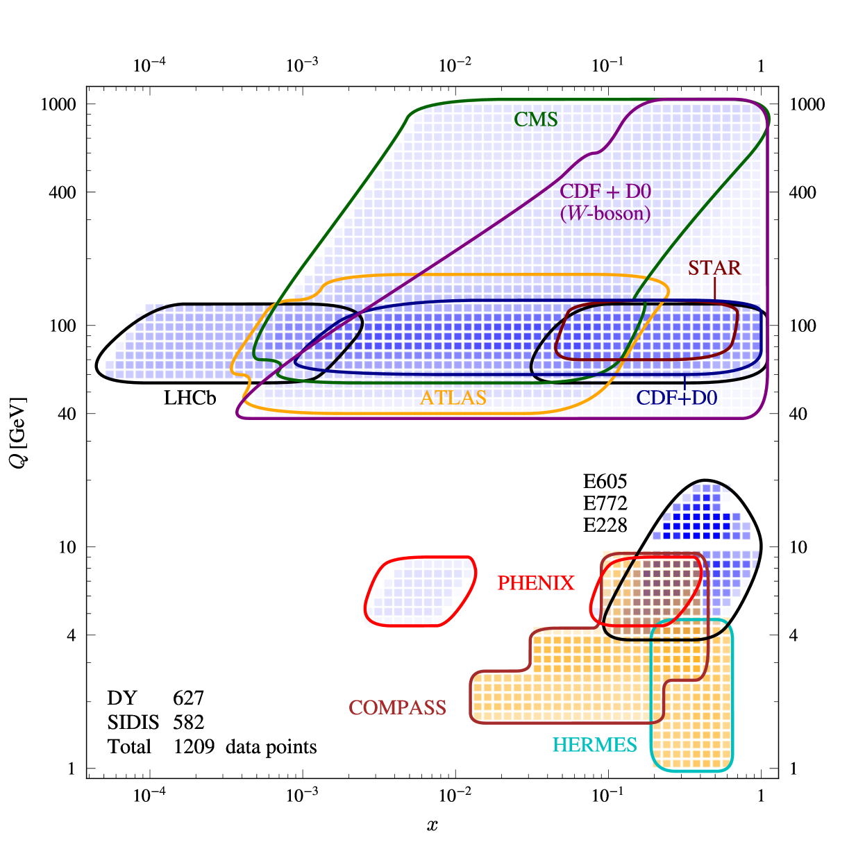
Figure 1: The kinematic range in $Q$ and $x$ covered by the used data. A darker shade indicates a denser distribution of data.

4 Fitting procedure

The fitting procedure and the method of estimation of uncertainties are identical to the ones employed in ART23 Moos:2023yfa , which in turn are inherited from our earlier studies Bury:2022czx ; Scimemi:2019cmh . For completeness, we present the main elements of this analyses here, referring the reader to the mentioned articles for any missing detail.

We use the standard definition of the $\chi^{2}$-test function adopted from the fits of collinear PDFs in refs. Ball:2008by ; Ball:2012wy . It is defined as

$$\chi^{2}_{test}=\sum_{i,j\in\text{data}}(m_{i}-t_{i})V^{-1}_{ij}(m_{j}-t_{j}),$$ (42)

where $i$ and $j$ run over all data points included in the fit, $m_{i}$ and $t_{i}$ are the experimental value and theoretical prediction for point $i$, respectively, and $V^{-1}_{ij}$ is the inverse of the covariance matrix. The covariance matrix is defined as

$$V_{ij}=\delta_{ij}\Delta_{i,\text{uncorr}.}^{2}+\sum_{l}\Delta_{i,\text{corr}.}^{(l)}\Delta_{j,\text{corr}.}^{(l)},$$ (43)

where $\Delta_{i,\text{uncorr}.}$ is the uncorrelated uncertainty of measurement $i$, and $\Delta_{i,\text{corr}.}^{(l)}$ is the $l$-th correlated uncertainty. If the data have a normalization uncertainty (usually due to the uncertainty in the measured luminosity), it is included in the $\chi^{2}$ as one of the correlated uncertainties. Such definition of the covariance matrix and the $\chi^{2}$-test function is also used, e.g., in the fits of the MAP collaboration Bacchetta:2022awv ; Bacchetta:2019sam ; Bacchetta:2024qre .

This definition of $\chi^{2}$ allows for a determination of correlated and uncorrelated contributions to the $\chi^{2}$-function  Ball:2012wy :

$$\chi^{2}=\chi^{2}_{D}+\chi^{2}_{\lambda},$$ (44)

where $\chi^{2}_{D}$ ($\chi^{2}_{\lambda}$) is the contribution due to the uncorrelated (correlated) uncertainties of the measurement. The mathematical definition of these terms can be found in ref. Ball:2012wy . This decomposition is often useful for analysis and visualization because the correlated (normalization) uncertainty is generally much larger than the uncorrelated one. Hence, in some plots, we show the comparison of the data with the part of prediction that contributes only to $\chi^{2}_{D}$ (and hence has “perfect” normalization). It allows to visually confirm the “goodness” of the $\chi^{2}$ values.

The ansätze for the TMD distributions and the CS kernel contain a total of 22 parameters, which we denote as $\overrightarrow{\lambda}$. To find the optimal values of $\overrightarrow{\lambda}$, we minimize the $\chi^{2}$ as a function of this vector. The resulting value, $\overrightarrow{\lambda}_{\text{center}}$, is called the central value fit. This central value can be used for quick estimations, but it lacks information about the correlation between parameters and uncertainties.

The estimation of uncertainties for the TMD distributions is the most time-consuming part of the computation. As in our earlier works, we employ the resampling method to carry out this task. We distinguish two sources of uncertainties: (i) the experimental uncertainties and (ii) the collinear PDF and FF uncertainties. Other sources of uncertainties (such as uncertainties in $M_{Z}$ or $\alpha_{s}$, or uncertainties due to missed higher perturbative orders) are considered negligible.

These two types of uncertainties are treated simultaneously in the analysis, but with different approaches. The experimental uncertainties are incorporated by performing fits to multiple instances of pseudo-data, which are created by adding Gaussian noise to the measured values. The description of the generation of pseudo-data can be found in ref. Ball:2008by . Simultaneously, the theoretical uncertainty from the collinear distributions is propagated by using a random independent replica (i.e., an element from the PDF/FF sample distribution) for the unpolarized PDFs, and for the FFs in the case of $\pi$ and $K$.

Each minimization results in the vector $\Lambda_{i}=\{\overrightarrow{\lambda}_{i},\overrightarrow{n}_{i}\}$, where $\overrightarrow{n}_{i}$ are three integers that identify the replicas of collinear distributions. The ensemble of $\Lambda$’s fully describes the TMD distributions and the CS kernel. This ensemble is then used in all further calculations. The list of values of $\Lambda_{i}$ can be found in the artemide repository artemide , in a format suitable for automatic processing by the DataProcessor. Notice that the $0$’th element of the set, $\Lambda_{0}$, is defined as the result of minimization for the central values of the data (without additional noise) and for the mean replicas, i.e., $\overrightarrow{n}_{0}=\overrightarrow{0}$.

Using the ensemble $\Lambda$, we can find then all type of quantities (TMD distributions, cross-sections, values of parameters, etc) and their associated uncertainties. For a quantity $F$, the procedure is as follows. We evaluate $F$ for each element $i$ of $\Lambda$, obtaining the ensemble $F_{i}=F[\Lambda_{i}]$. The mean value is then the mean $\langle F_{i}\rangle$, and the 68% confidence interval (CI) uncertainty band is found by the resampling method by computation of the 16% and 84% quantiles. The procedure described above allows to correctly propagate all correlations. Notice that for ideal (symmetric and independent) distributions the mean value would coincide with the central one. However, naturally one has $\langle F[\Lambda_{i}]\rangle\neq F[\Lambda_{0}]$, due to the correlations between members of $\Lambda$, asymmetries etc. Nonetheless, for many tests we employ central values assuming that they are close enough to the mean values. The reason is that the computation of the central value requires only one minimization while the computation of the mean requires multiple minimizations.

The computation of the theoretical predictions and related values (such as TMMs) for a given set of NP parameters is done by artemide (v.3.01), which is publicly available at artemide . artemide has a PYTHON interface, which is used to compute the $\chi^{2}$ value with the DataProcessor library DataProcessor . The minimization is made with the iminuit package iminuit . The analysis program and supplementary codes, together with the collection of the experimental data points can be found in DataProcessor .

5 Results

In this section, we present the results of our fit. We begin by discussing technical aspects such as the values of the non-perturbative parameters and the quality of the data description. We then move on to the discussion of the physical results. We provide a detailed presentation of the CS kernel, TMDPDF, and TMDFF in both position and momentum space, including comparisons with their earlier determinations. Finally, we discuss the values of the zeroth and second TMMs obtained from our extraction. Due to the large number of graphical materials, some plots are presented in the appendices. In particular, appendix A contains a collection of plots comparing our results with the data, while appendix B provides a collection of plots comparing TMDPDF and TMDFFs from different extractions.

5.1 Values for non-perturbative parameters

We begin by presenting the values of the NP parameters along with their uncertainties in table 4. These values are obtained from the parameter distribution as the mean and the 68%CI, following the procedure outlined in the previous section.

From the table, one can see that the TMDPDF parameters $\lambda_{1}^{i}$ are well determined. The same applies to $\lambda_{2}^{u}$ and $\lambda_{2}^{d}$. In contrast, $\lambda_{2}^{\text{sea}}$ is poorly constrained, with its lower uncertainty being comparable in size to its mean value. Interestingly, $\lambda_{2}^{\bar{u}}$ deviates from the typically small values of the other $\lambda_{2}$ parameters. As we demonstrate later, this larger value leads to some undesired features in the distributions (e.g., an unrealistically large second TMM at $x\sim 0.1$). A similarly large $\lambda_{2}^{\bar{u}}$ was also observed in the ART23 fit. At present, it is difficult to determine whether this behavior genuinely reflects a property of the anti-up quark TMDPDF or if it serves to compensate for the collinear distribution. The $\lambda_{3}^{i}$ parameters also exhibit similar mean values, with the up-quark parameter having smaller uncertainties.

Regarding the parameters associated with the pion TMDFF, the values of $\eta_{1}^{\pi,j}$ are of similar magnitude ($\sim 0.6$), except for the down-quark parameter, which is not well determined, and $\eta_{1}^{\pi,r}$. This is expected, as collinear FFs typically distinguish between valence quarks, sea quarks, heavy quarks, and gluons, while in this case, we are grouping the latter three contributions together with other sea densities. Current TMD SIDIS data are not sensitive enough to allow further differentiation, but in the future, it may be possible to separate the “rest” into individual TMD densities. A similar pattern is observed for the kaon TMDFFs.

	Collins-Soper kernel
Parameter	$c_{0}$			$c_{1}$
Value	$0.0859^{+0.0023}_{-0.0017}$			$0.0303^{+0.0038}_{-0.0041}$
	Unpolarized TMDPDF
Parameter	$\lambda_{1}^{u}$	$\lambda_{2}^{u}$	$\lambda_{3}^{u}$	$\lambda_{2}^{\bar{u}}$
Value	$0.486^{+0.048}_{-0.049}$	$0.041^{+0.007}_{-0.036}$	$5.26^{+0.54}_{-0.77}$	$21.1^{+1.5}_{-4.2}$
Parameter	$\lambda_{1}^{d}$	$\lambda_{2}^{d}$	$\lambda_{3}^{d}$	$\lambda_{2}^{\bar{d}}$	$\lambda_{1}^{sea}$	$\lambda_{2}^{sea}$
Value	$0.569^{+0.035}_{-0.045}$	$0.15^{+0.01}_{-0.11}$	$7.7^{+2.0}_{-4.5}$	$0.16^{+0.01}_{-0.15}$	$0.240^{+0.035}_{-0.083}$	$0.07^{+0.00}_{-0.07}$
	Unpolarized TMDFF for $\pi$
Parameter	$\eta_{0}^{\pi}$		$\eta_{1}^{\pi,u}$	$\eta_{1}^{\pi,\bar{d}}$	$\eta_{1}^{\pi,\bar{u}}$	$\eta_{1}^{\pi,r}$
Value	$0.696^{+0.011}_{-0.006}$		$0.626^{+0.047}_{-0.027}$	$0.003^{+0.081}_{-0.080}$	$0.610^{+0.028}_{-0.028}$	$-0.47^{+0.14}_{-0.18}$
	Unpolarized TMDFF for $K$
Parameter	$\eta_{0}^{K}$		$\eta_{1}^{K,u}$	$\eta_{1}^{K,\bar{s}}$	$\eta_{1}^{K,\bar{u}}$	$\eta_{1}^{K,r}$
Value	$0.884^{+0.020}_{-0.032}$		$0.882^{+0.055}_{-0.147}$	$1.74^{+0.16}_{-0.28}$	$1.15^{+0.11}_{-0.28}$	$-0.10^{+0.36}_{-0.30}$

Table 4: Mean values of parameters obtained in the fit and their uncertainties, obtained from the distribution of replicas.

The correlation matrix of the parameters is presented in Fig. 2. Several features of this matrix are worth highlighting:

• Parameters $c_{0}$ and $c_{1}$ are highly correlated, which is expected since $c_{1}$ was introduced to fine-tune the CS kernel for high-energy experiments. It is possible to achieve a “good” fit using a single parameter.

• Within its own block, the parameters for each TMDFF are strongly correlated. In both cases ($\pi$ and $K$), the general scale parameter $\eta_{0}$ is highly correlated with the valence parameter $\eta_{1}^{u}$. This is likely because the SIDIS data are concentrated in a limited kinematical range, making them insensitive to the wide-range characteristics of the distributions.

• In general, all distributions are anti-correlated with the parameters $c_{0,1}$. This is natural since the CS kernel introduces a global suppression factor, which can also be mimicked by the non-perturbative parts of the distributions. A distinctive feature of the CS kernel is its non-trivial dependence on $Q$. Typically, large-$Q$ data have reduced sensitivity to large-$b$ values (i.e., $b\gtrsim 1$–$1.5$ GeV^-1).

• The parameter blocks for the TMDPDF and TMDFF are practically uncorrelated, which is a positive characteristic. The most correlated parameter pairs are $(\lambda_{1}^{u},\eta_{1}^{K\bar{u}})$ and $(\lambda_{1}^{d},\eta_{1}^{K\bar{s}})$. The first correlation arises from fine-tuning the $K^{-}$-production data, while the second is an indirect effect caused by internal correlations within the TMDFF block.

• There is a significant anti-correlation between $\pi$ and $K$ blocks, due to the COMPASS data being measured with $h=\pi+K$.

Generally, the correlation matrix demonstrate that the parametrical form of the distributions is sufficiently consistent.

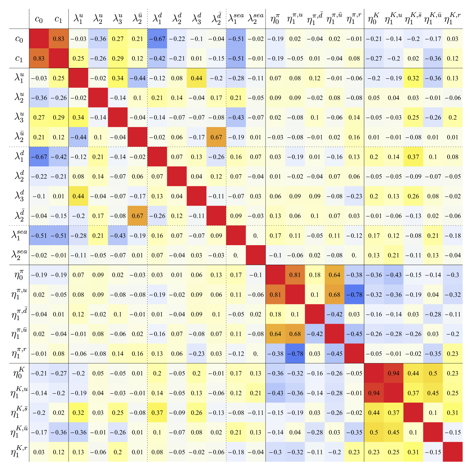
Figure 2: Correlation matrix for parameters of the fit.

5.2 Quality of the data description

Let us now examine the quality of the data description, as quantified by the $\chi^{2}$ value. The breakdown of $\chi^{2}$ across different data subsets is presented in table 5. This table can be compared with analogous tables from previous fits, including SV19, ART23, Pavia19, MAP22, and MAP24, showing overall agreement between with them. The reported values correspond to $\chi^{2}$ calculations using the mean values of the parameters listed in table 4.

Data set	$N_{\text{pt}}$	$\chi_{D}^{2}/N_{\text{pt}}$	$\chi_{\lambda}^{2}/N_{\text{pt}}$	$\chi^{2}/N_{\text{pt}}$
CDF	84	2.06	0.07	2.13
D0	36	2.20	0.08	2.28
ATLAS	49	1.43	0.25	1.68
CMS	113	0.69	0.13	0.82
LHCb	68	1.06	0.26	1.32
PHENIX	3	0.41	0.08	0.48
STAR	11	1.15	0.16	1.32
DY collider total:	364	1.34	0.15	1.49
E228	175	0.67	0.02	0.69
E772	35	1.25	0.12	1.37
E605	53	0.31	0.12	0.42
DY fixed-target total:	263	0.67	0.05	0.73
DY total:	627	1.06	0.11	1.17
HERMES $\pi^{+}$	48	1.62	0.08	1.70
HERMES $\pi^{-}$	48	1.17	0.12	1.29
HERMES $K^{+}$	48	0.47	0.00	0.47
HERMES $K^{-}$	48	1.31	0.03	1.34
COMPASS $h^{+}$	195	0.65	0.02	0.67
COMPASS $h^{-}$	195	0.91	0.00	0.91
SIDIS total:	582	0.90	0.02	0.92
Total:	1209	0.98	0.07	1.05

Table 5: Breakdown of $\chi^{2}$ values for different experiments. $N_{\text{pt}}$ is the number of points in the data sub-set. $\chi_{D}^{2}$ and $\chi_{\lambda}^{2}$ are the components associated with contribution to $\chi^{2}$ due to disagreement in the shape (uncorrelated uncertainties) and normalization (correlated uncertainties), correspondingly. The numbers are obtained using the mean values of the parameters.

The total resulting $\chi^{2}/N_{\text{pt}}$ is

$$\frac{\chi^{2}}{N_{\text{pt}}}=1.17_{\text{ DY}}\oplus 0.92_{\text{ SIDIS}}=1.05.$$ (45)

We emphasize that this value is computed using the mean values of the parameters. The central value fit (i.e. the fit to the undisturbed data with only central replica of collinear distributions) results into

$$\text{central value fit:}\qquad\qquad\frac{\chi^{2}}{N_{\text{pt}}}=1.16_{\text{ DY}}\oplus 0.86_{\text{ SIDIS}}=1.01~.$$ (46)

It is also instructive to consider the DY and SIDIS data sets separately. Naturally, the values of $\chi^{2}$ for these fits are smaller. We obtained

$$\text{separate fits:}\qquad\frac{\chi^{2}}{N_{\text{pt}}}\Big{|}_{\text{ DY-only}}=1.02,\qquad\frac{\chi^{2}}{N_{\text{pt}}}\Big{|}_{\text{ SIDIS-only}}=0.79.$$ (47)

Simultaneously, if we use the values of parameters obtained in separate fits for other set (i.e. the values obtained in SIDIS-only fit for DY data, or values of TMDPDFs obtained in DY-only fit for SIDIS data) we obtain $\chi^{2}/N_{\text{pt}}\sim 2-3$. Due to it, we conclude that in the simultaneous fit of DY and SIDIS it is important to balance the different parts of the NP ansatz.

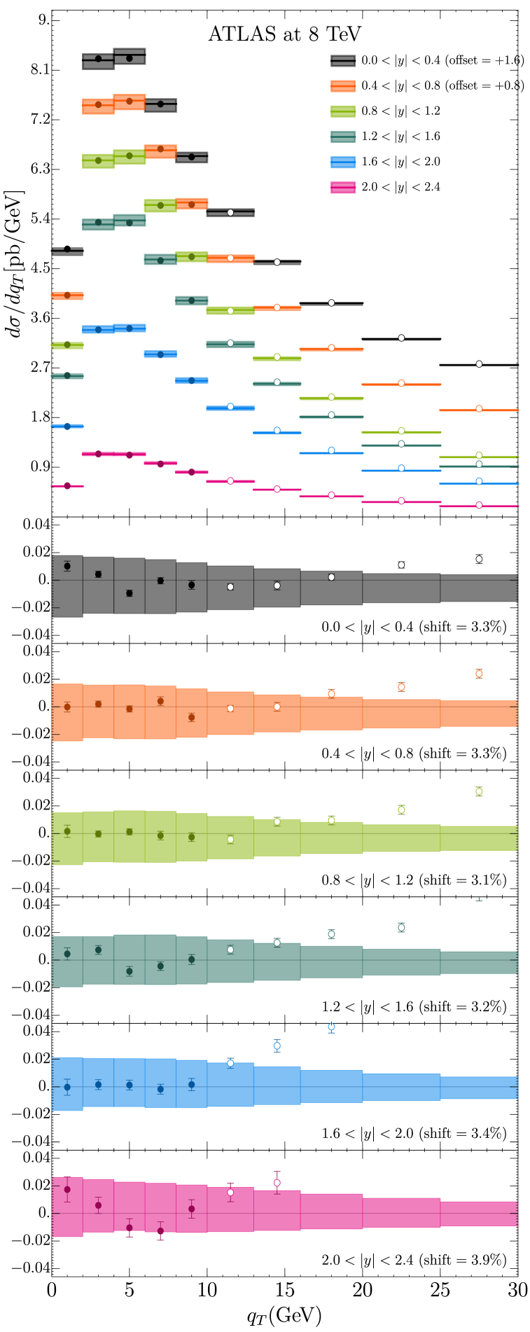
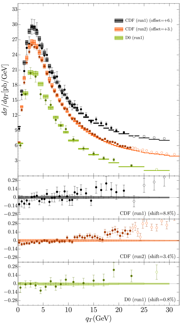
Figure 25: Left panel: comparison of ART25 prediction with measurements of Z-boson production at different values of rapidity made by ATLAS at $\sqrt{s}=8$ TeV ATLAS:2015iiu . Right panel: comparison of ART25 prediction with measurements of Z-boson production at Tevatron CDF:1999bpw ; CDF:2012brb ; D0:2007lmg .

The plots comparing data with theoretical predictions are presented in appendix A. The typical uncertainty band for DY in the vicinity of the $Z$-boson mass is around 2%. In some cases, it is significantly larger than the uncertainty of the data points (see the ATLAS measurements in fig. 25 and 27). According to detailed studies in refs. Bury:2022czx ; Moos:2023yfa , the dominant source of this uncertainty is the collinear PDF uncertainty, which cannot be reduced within the present fit. For the SIDIS data, the typical uncertainty is around 5%. These uncertainty bands account only for non-perturbative parameters and collinear inputs, and do not include uncertainties arising from missing higher-order perturbative corrections or other theoretical sources.

5.3 Limits of data description

We observe an excellent description of both DY and SIDIS data included in the fit (represented by filled points in the plots). Moreover, in many cases, the theoretical predictions accurately capture the behavior of data even beyond the applicability range of the factorization theorem (these points are shown as empty circles). In general, for points with $\delta>0.25$, the theoretical predictions tend to fall below the data, which is a well-known property of the TMD factorization approach.

To systematically test the limits of TMD factorization, we performed multiple fits with different values of the cut parameter $\delta$ (only considering central fits). The corresponding values of $\chi^{2}/N_{\text{pt}}$ are shown in Fig. 3. It is evident that the agreement with the theory decreases significantly for $\delta>0.25$. Interestingly, for SIDIS measurements the level of disagreement grows faster. This result confirms that our choice of $\delta=0.25$ is supported by the data. The same test and conclusion were also reported in refs. Scimemi:2017etj ; Scimemi:2019cmh ; Bacchetta:2019sam ; Bacchetta:2022awv .

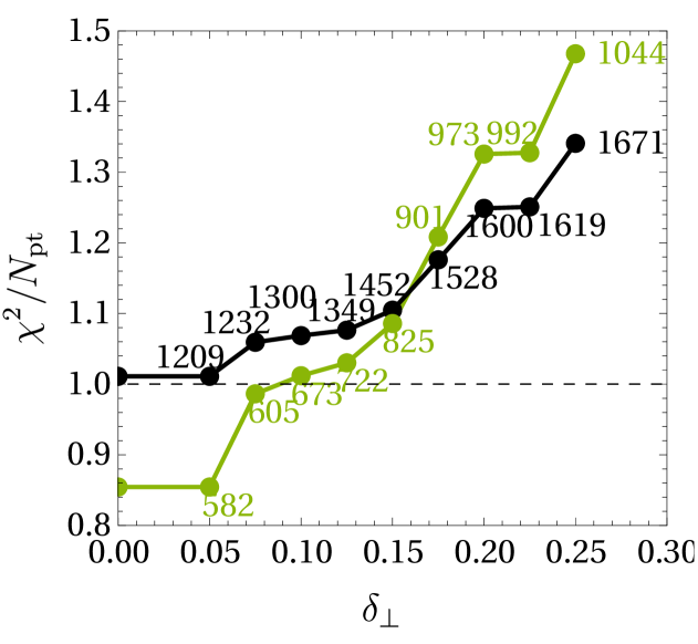
Figure 3: The values of $\chi^{2}/N_{\text{pt}}$ obtained for fits with sets of data selected with different values of cut parameters $\delta$, eq. (37), and $\delta_{\perp}$, eq. (48). The black (orange, green) points indicate the values for total (only DY, only SIDIS) data set. The numbers indicate the number of data points for each case.

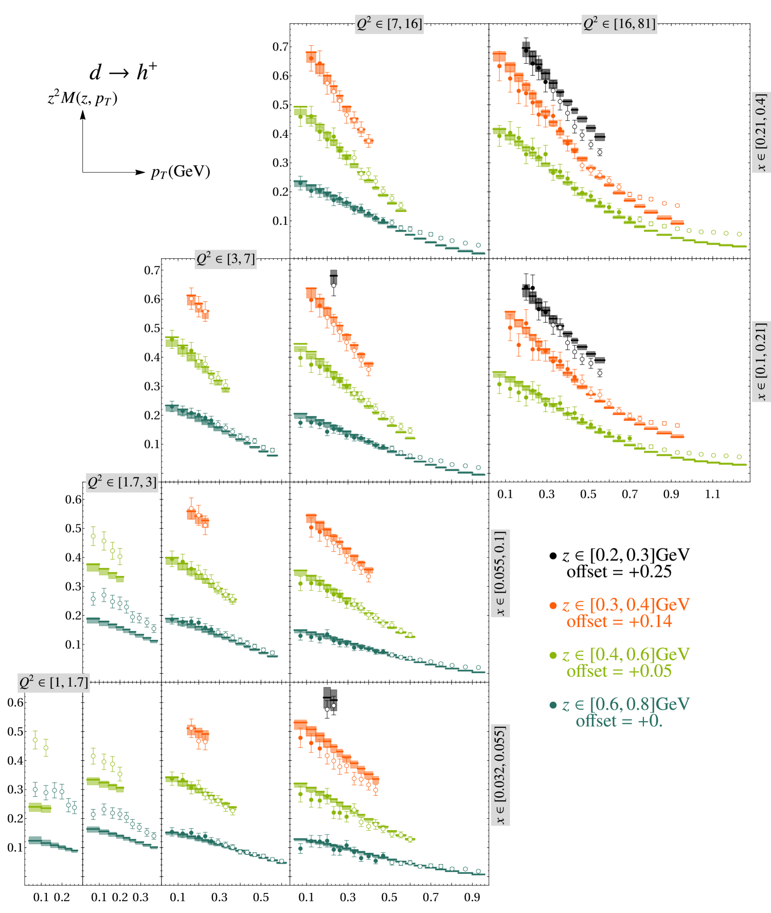
Figure 30: Comparison of ART25 prediction for $h^{+}$ production in SIDIS measured at COMPASS COMPASS:2017mvk . For better visibility, points with different bins in $z$ are shifted by a common value indicated in the legend. The bins with lower values of $x$ are shown in fig. 32.

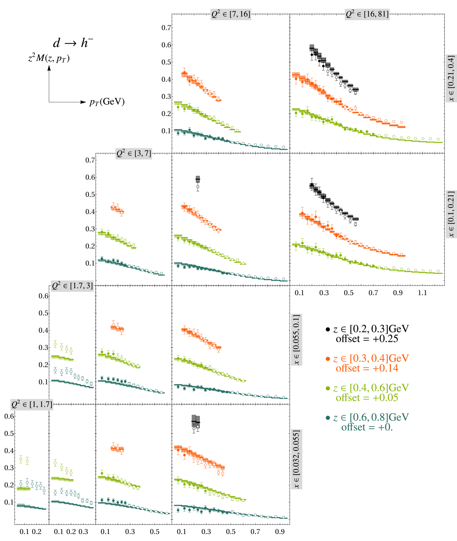
Figure 31: Comparison of ART25 prediction for $h^{-}$ production in SIDIS measured at COMPASS COMPASS:2017mvk . For better visibility, points with different bins in $z$ are shifted by a common value indicated in the legend. The bins with lower values of $x$ are shown in fig. 32.

We also observed that, for some SIDIS measurements, data points with lower $z$ are well described over a larger range (see, for instance, figures 30 and 31). This suggests the possibility that TMD factorization remains valid at higher values of $p_{\perp}$, contrary to theoretical expectations. To test this hypothesis, we performed fits for SIDIS data (with fixed uTMDPDF and DY parts), including additional SIDIS data points with

$$\delta_{\perp}=\langle p_{\perp}\rangle/\langle Q\rangle$$ (48)

below a certain threshold, in addition to the main dataset selected with $\delta<0.25$. This is similar to the selection criterion used in fits by the MAP collaboration Bacchetta:2022awv ; Bacchetta:2024qre . The corresponding values of $\chi^{2}/N_{\text{pt}}$ are shown in the right panel of fig. 3. This plot demonstrates that including such points leads to an increase in $\chi^{2}$ without a plateau. Consequently, such a selection criterion does not agree with the TMD factorization approach.

Inspecting the plots comparing theory predictions with SIDIS data, one can observe that the predictive power of the theory deteriorates for $Q<2$ GeV. Already at $\sim 1.5$ GeV, the theoretical predictions are almost a factor of two smaller than the data. This discrepancy is particularly pronounced in the COMPASS data and is most likely due to larger target-mass corrections in the charged hadron case, which includes the proton.

Additionally, it is important to notice that the current description omits the $F_{UU,L}$ component of the SIDIS cross-section, which vanishes at leading power. At typical SIDIS energies ($Q\sim 2-4$ GeV), this structure function can be comparable in magnitude to the leading-power term. Incorporating this contribution into the analysis would require updating the theoretical formalism, for example, by including power correction terms, as has been done for the DY process in refs. Vladimirov:2023aot ; Piloneta:2024aac .

5.4 The CS kernel

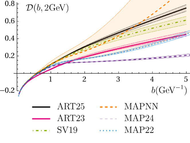
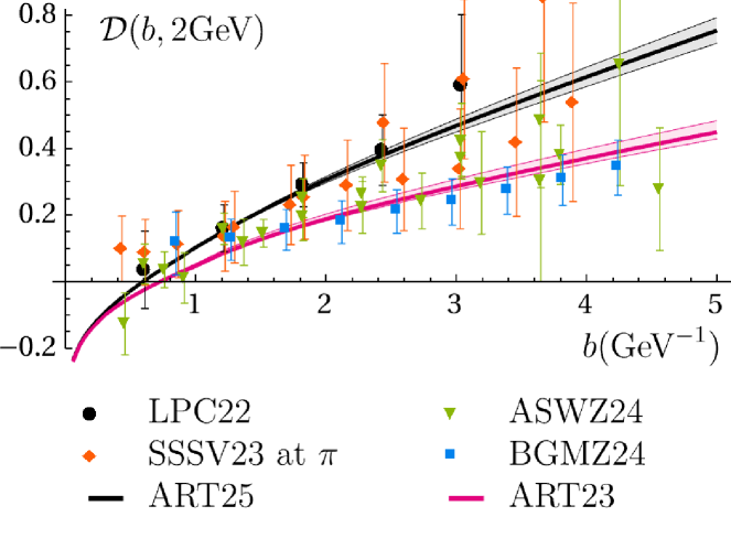
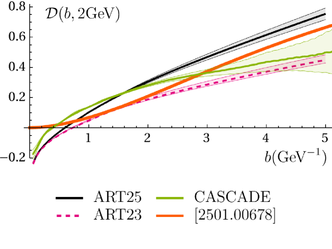
Figure 4: Comparison of the CS kernel extracted in this work (labeled as ART25) with other determinations, namely: (upper left panel) extraction from fits of data made in refs. Moos:2023yfa (ART23), Scimemi:2019cmh (SV19), Bacchetta:2025ara (MAPNN), Bacchetta:2024qre (MAP24) and Bacchetta:2022awv (MAP22); (upper right panel) lattice computations performed in refs. Bollweg:2024zet (BGMZ24), Avkhadiev:2023poz ; Avkhadiev:2024mgd (ASWZ24), Shu:2023cot (SSSV23), LatticePartonLPC:2022eev (LPC22). For the SSSV23 analyses only the extraction made with pion are presented for clarity; (lower panel) model computations of CS kernel. The curve CASCADE correspond to the CS kernel used in the parton branching approach within the CASCADE generator CASCADE:2021bxe ; BermudezMartinez:2020tys determined by the method of ref. BermudezMartinez:2022ctj . The orange line shows the result of the computation of the CS kernel in the instanton vacuum model Liu:2024sqj .

In fig. 4 we present the value of the CS kernel determined in this work (labeled as ART25) in comparison with other extractions from experimental data made in refs. Moos:2023yfa ; Scimemi:2019cmh ; Bacchetta:2025ara ; Bacchetta:2024qre ; Bacchetta:2022awv , with the lattice simulations made in refs. Bollweg:2024zet ; Avkhadiev:2023poz ; Avkhadiev:2024mgd ; Shu:2023cot ; LatticePartonLPC:2022eev , and with other theoretical approaches (parton shower CASCADE:2021bxe ; BermudezMartinez:2020tys , instanton vacuum model Liu:2024sqj ). In all cases we selected only the most recent extractions. The comparison with earlier works, such as refs. Bacchetta:2019qkv ; Bacchetta:2017gcc ; Bertone:2019nxa ; Scimemi:2017etj ; Shanahan:2020zxr ; BermudezMartinez:2022ctj ; LatticeParton:2020uhz ; Schlemmer:2021aij ; Shanahan:2021tst , is not presented.

Comparison with other extractions reveals that determinations of the CS kernel fall into two distinct groups. The first group (ART23, MAP22, MAP24) prefers a lower value of the CS kernel and aligns well with lattice simulation Avkhadiev:2024mgd (ASWZ24). The second group (ART25, SV19, MAPNN) obtains a CS kernel that is nearly twice as large for $b\geq 0.5$ GeV^-1. Despite the significant uncertainties in lattice data, both groups remain consistent with lattice simulations.

The larger CS kernel obtained in the present fit is primarily driven by the influence of SIDIS data, which is also observed in the SV19 extraction. These data push the CS kernel to higher values while compensating for this shift through fine-tuning of the TMDPDF parameters. In contrast, the MAP22 and MAP24 analyses might be less sensitive to this effect because they employ a special procedure for normalizing the SIDIS data, which impacts the CS kernel determination. In general, extractions incorporating SIDIS data are expected to be more reliable, as lower-$q_{T}$ measurements provided by SIDIS data are more sensitive to larger $b$. Extractions based solely on DY data have lower sensitivity to this region and may therefore be more susceptible to model biases. The possibility to have a model bias in DY-only extractions is further supported by the fact that a neural-network-based extraction using only DY data (MAPNN) also predicts a larger CS kernel.

Comparing different extractions, we observe that the typical uncertainty in the CS kernel is smaller than that the uncertainty band obtained in MAPNN. This is a clear manifestation of a model bias, which restricts the variation of parameters by imposing strong constraints at small $b$. As a result, the model-driven extrapolation to larger $b$ values also inherits a reduced uncertainty. This observation suggests that the uncertainty bands reported in SV19, ART23, and the present work may be underestimated for $b>$1-2 GeV^-1. A deeper investigation of this issue is deferred to a future work.

5.5 TMD distributions in position space

The 3-dimensional plots of the TMDPDFs in $b$-space are shown in fig. 5, where we present the results for the $u$, $d$, and $\bar{u}$ flavors. Other sea flavors exhibit similar shapes to that of the $\bar{u}$-flavor, and thus we omit them for brevity. The sections of the optimal TMDPDFs at fixed values of $x=0.01$ (left) and $x=0.1$ (right) are shown in fig. 6. For clarity, some distributions in the left panel have been vertically displaced by a fixed amount, as indicated in the figure. To provide a clearer picture of the uncertainties, fig. 7 displays the ratio of the uncertainties to the corresponding TMDPDF mean values.

It is clearly visible from the right panel of fig. 5 that the size of $\bar{u}$ TMDPDF at $x\sim 0.1$ is abnormally small compared to other flavors. This discrepancy reflects the fact that $\lambda_{2}^{\bar{u}}$ is very distinct from the remaining $\lambda_{2}$’s. Simultaneously, the uncertainty of the $\bar{u}$ TMDPDF at $x=0.1$ is of the same absolute size, leading to an inflated relative uncertainty. We attribute this effect to some minor instability in the collinear distribution, which is overcompensated in the TMD fit. Although this effect does not significantly impact the observables, it has a large impact in the determination of $\bm{k}_{T}^{2}$ (see sec. 5.8 for a discussion).

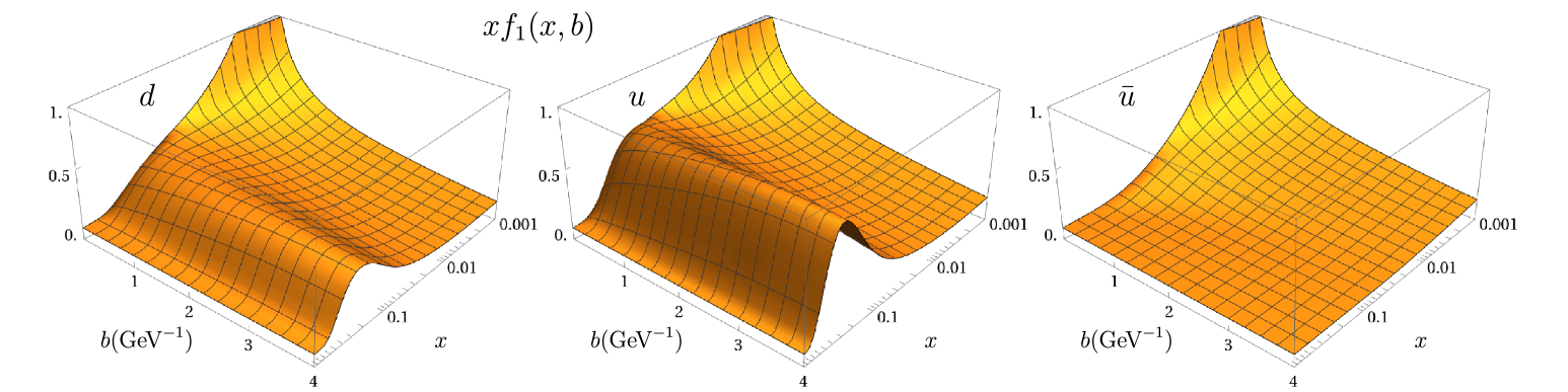
Figure 5: Optimal unpolarized TMDPDF as a function of $(x,b)$ for down (left), up (centre) and anti-up (right) quarks. The mean values, without uncertainties are presented.

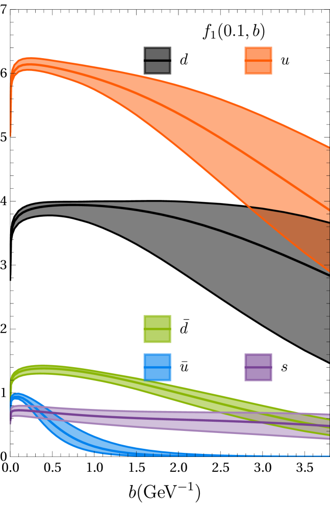
Figure 6: Optimal unpolarized TMDPDFs as a function of $b$ at fixed $x$. For better visibility some of the curves are shifted by a constant off-set indicated in the plot.

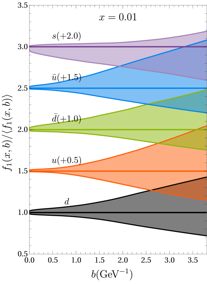
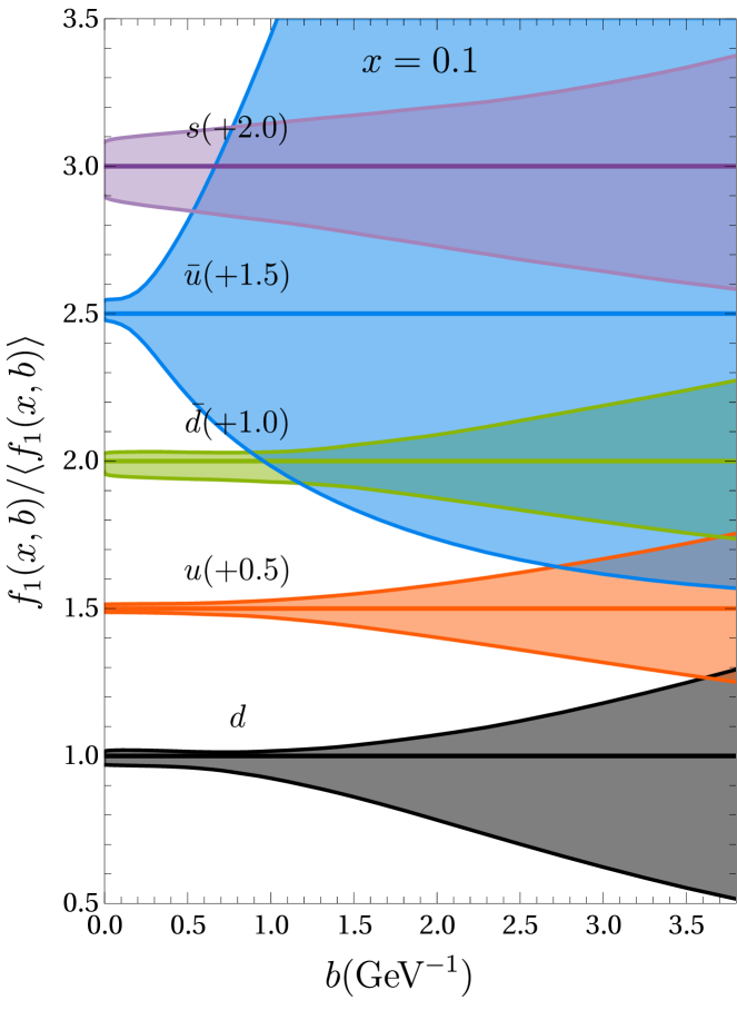
Figure 7: The ratio of the optimal unpolarized TMDPDFs to their mean values as a function of $b$ at fixed $x=0.01$ (left) and $x=0.1$ (right). For better visibility the curves are shifted by a constant off-set indicated in the plot. The color code for the distributions is the same as in fig. 6.

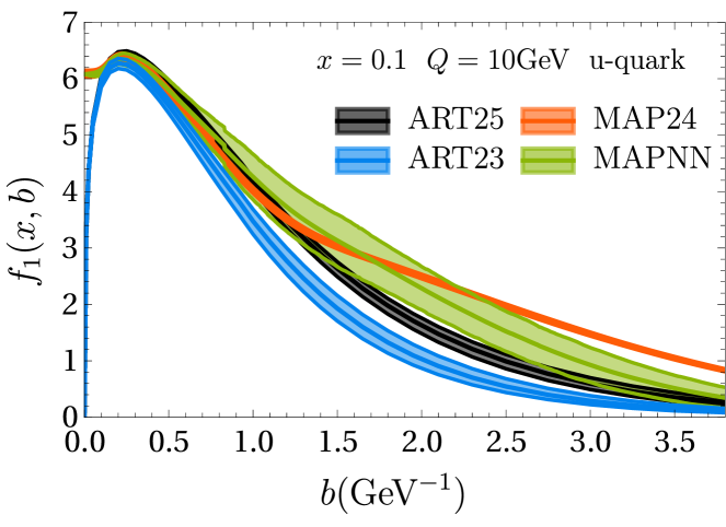
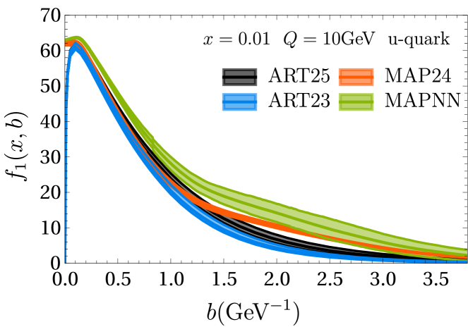
Figure 8: Comparison of unpolarized TMDPDF for u-quark at $x=0.1$ and $x=0.01$ with extractions made in refs. Moos:2023yfa (ART23), Bacchetta:2025ara (MAPNN) and Bacchetta:2024qre (MAP24). The comparison is done for TMD distributions evaluated at 10 GeV.

The equivalent plots for the TMDFFs are shown in fig. 9. It is evident that the shapes of the TMDPDFs and TMDFFs differ. Most of these disparities arise from the differences in the collinear functions used as the baseline. However, the choice of different ansätze for the non-perturbative parts also contributes to the final results. For all “rest” contributions (comprising all sea quarks except for $\bar{u}$), the distributions turn negative at some value of $b$ (e.g., the $s$-quark distribution in $\pi^{+}$ in fig. 9). This occurs due to the negative values of the parameters $\eta_{1}^{h,r}$ (see table 4). This behavior does not pose any practical or theoretical issues, since there is no positivity constraint for TMD distributions in $b$-space (nor in $k_{T}$-space).

Notably, the $\bar{s}$ TMDFF in the kaon is significantly larger than all other distributions. This feature is inherited from the collinear part, as highlighted in the comparisons of flavors in MAPFF1 AbdulKhalek:2022laj . The profiles of the TMDFFs, along with their uncertainty bands, are shown in Fig. 10 for $z=0.3$. The uncertainty bands for the TMDFFs are several times larger than those for the TMDPDFs.

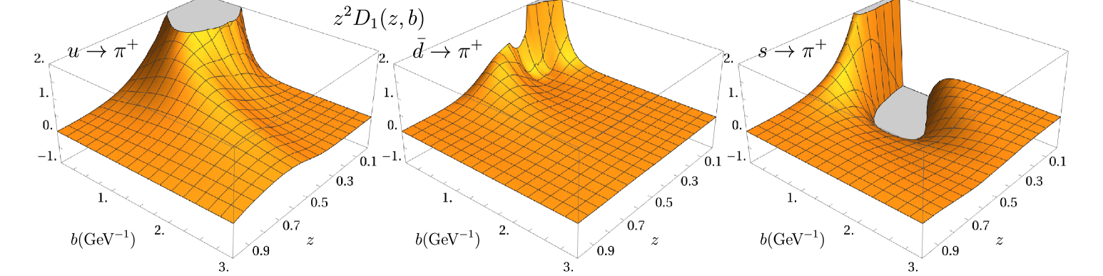
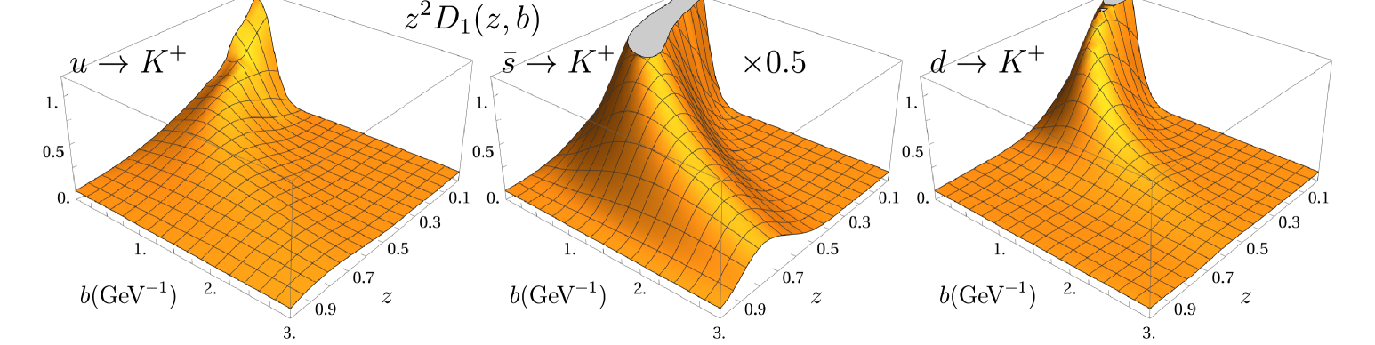
Figure 9: Optimal unpolarized TMDFFs for $\pi^{+}$ (upper row) and for $K^{+}$ (lower row) as a function of $(x,b)$. The mean value is presented.

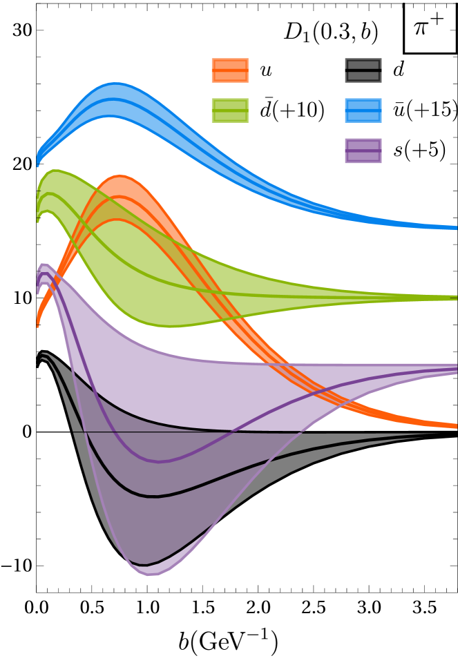
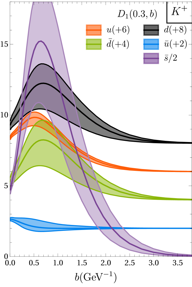
Figure 10: Optimal unpolarized TMDFFs as a function of $b$ at fixed $z=0.3$. For better visibility some of curves are shifted by a constant off-set indicated in the plot. The $\bar{s}$ distribution in kaon is divided by 2.

In fig. 8 and 11, we present a comparison of our extraction with earlier results from ref.Moos:2023yfa ; Bacchetta:2022awv ; Bacchetta:2025ara ; Bacchetta:2024qre . It is important to notice that the extractions by the MAP collaboration are performed using the NangaParbat code, which employs a different scale setup. Specifically, the $b_{\text{min}}$-prescription is used, which modifies the evolution at small-$b$. This difference is responsible for the contrasting behavior of the curves at $b\lesssim 0.2$ GeV^-1. In the intermediate region $b\sim 0.2-1$ GeV^-1, the TMDPDF values are in general agreement. However, for larger values of $b$, the curves differ again. This deviation does not indicate a discrepancy between the extractions, as the data are generally insensitive to this region. Therefore, we conclude that there is overall agreement between our extraction of the TMDPDFs and those from earlier works.

The TMDFFs distributions are shown in fig. 11 and they exhibit much less agreement. This is understandable given that TMDFFs appear only in SIDIS and there are significant theoretical differences in the description of SIDIS data between our groups.

A larger number of plots comparing different extractions are presented in appendix B.

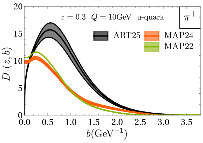
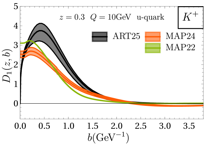
Figure 11: Comparison of unpolarized TMDPDF for u-quark at $x=0.1$ and $x=0.01$ with extractions made in refs. Bacchetta:2022awv (MAP22) and Bacchetta:2024qre (MAP24). Comparison is done for TMD distributions evaluated at 10 GeV.

5.6 TMD distributions in momentum space

TMD distributions are naturally defined in position space; however, the Fourier transform of the TMDPDF is interpreted as the 3D momentum $xp^{+}+\bm{k}_{T}$ carried by the quark in the hadron, and similarly for the TMDFF. They are defined as

$$f_{1}(x,\bm{k}_{T};\mu,\zeta)=\int\frac{d^{2}\bm{b}}{(2\pi)^{2}}e^{i(\bm{b}\bm{k}_{T})}f_{1}(x,\bm{b};\mu,\zeta),$$ (49)

and analogously for the TMDFF.

The density plots of unpolarized TMDPDFs are shown in fig. 12. These figures clearly illustrate the expectations of the parton model; for instance, the transverse momentum increases as $x$ decreases, and the momentum of sea quarks is negligible compared to that of valence quarks for $x\gtrsim 0.1$. It is important to notice that the density plots do not reflect the size of the uncertainty, which is particularly large at $k_{T}\sim 0$. The profiles with uncertainty bands in momentum space are presented in fig. 13 for $x=0.1$ (left), $x=0.01$ (center), and $x=0.001$ (right). The oscillations in the uncertainty band for the $s$-quark are a result of limited statistics.

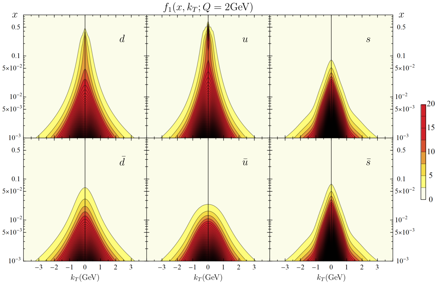
Figure 12: The contour plot of unpolarized TMDPDFs for various quark flavors in proton as a function of $x$ and $k_{T}$ at $\mu=\sqrt{\zeta}=2$ GeV scale.

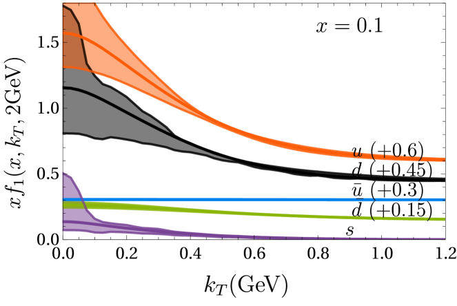
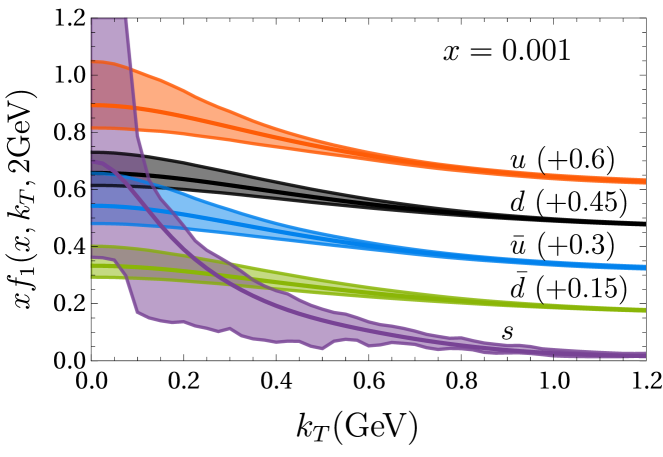
Figure 13: The plot of unpolarized TMDPDF distributions for different quark flavors in proton as a function of $k_{T}$ at fixed values of $x$ and scales $\mu=\sqrt{\zeta}=2$ GeV. For better visibility the curves have constant offsets, indicated in parentheses.

The analogous plots for TMDFFs are shown in fig. 14 and 15. These distributions are clearly distinct from the TMDPDF case. The width of the $k_{T}$ distribution grows much faster for the fragmentation functions, a feature consistently observed across all flavors for both pions and kaons. In the case of pions, some distributions are negative near $k_{T}=0$, which contradicts the naive expectation. We would like to emphasize that, despite their negative values in momentum space, all distributions correctly reproduce the collinear FF once integrated over $k_{T}$ (see sec. 5.7). The uncertainty bands for $D_{1}(z,\bm{k}_{T})$ are presented in fig. 16.

The contribution of the $\bar{s}$ quark in the kaon is the largest by almost an order of magnitude. This behavior is mainly due to the very large collinear FF (which is correctly reconstructed from TMDFF). If this picture is appropriate, one can interpret it as the $\bar{s}$ quark carrying the most part of the kaon momentum, and being mostly collinear (because its $\bm{k}_{T}$ distribution drops faster than other distributions).

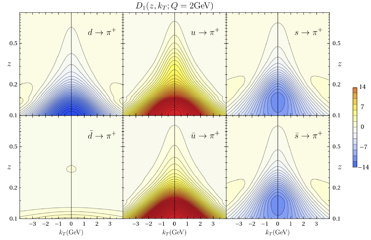
Figure 14: The contour plot of unpolarized TMDFF for various quark flavors in the positive pion as a function of $z$ and $k_{T}$ at $\mu=\sqrt{\zeta}=2$ GeV scale.

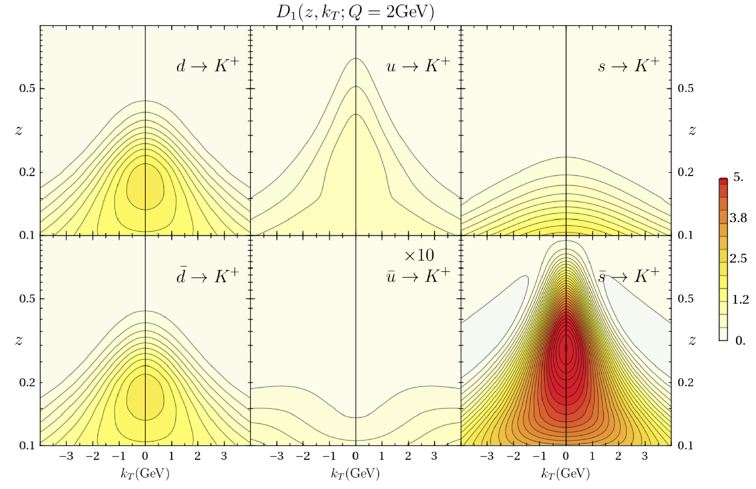
Figure 15: The contour plot of unpolarized TMDFF for various quark flavors in the positive kaon as a function of $z$ and $k_{T}$ at $\mu=\sqrt{\zeta}=2$ GeV scale.

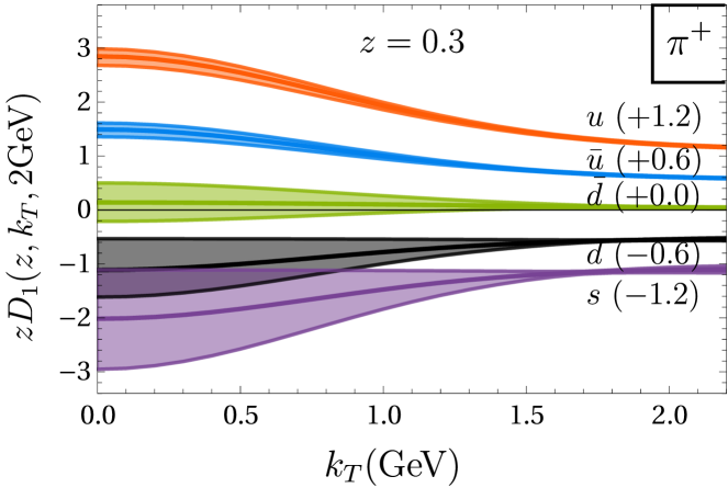
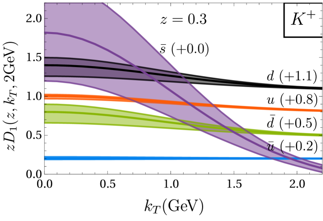
Figure 16: The plot of unpolarized TMDFF distributions for $\pi^{+}$ and $K^{+}$ for different quark flavors as a function of $k_{T}$ at fixed value of $z=0.3$ and scales $\mu=\sqrt{\zeta}=2$GeV. For better visibility the curves have constant offsets, indicated in parentheses.

5.7 Restoration of collinear distributions from TMD distributions

TMD distributions can be used to define collinear densities computing the zeroth transverse momentum moment (TMM). The resulting function is a collinear distribution computed in the so-called TMD-scheme. The translation to the ordinary $\overline{\text{MS}}$-scheme can be done by convoluting with a finite renormalization constant $Z$. Explicitly, the relation reads

$$f_{1,q\leftarrow h}(x,\mu) = \sum_{f^{\prime}}Z_{f\leftarrow f^{\prime}}(x,\mu)\otimes\int^{\mu}d\bm{k}_{T}^{2}f_{1,f^{\prime}\leftarrow h}(x,\bm{k}_{T}),$$ (50)

$$d_{1,f\to h}(z,\mu) = \sum_{f^{\prime}}Z_{f\to f^{\prime}}(z,\mu)\otimes\int^{\mu}d\bm{k}_{T}^{2}D_{1,f^{\prime}\to h}(x,\bm{k}_{T}),$$ (51)

where $f_{1}(x,\bm{k}_{T})$ and $D_{1}(x,\bm{k}_{T})$ are the optimal TMDPDF and TMDFF in momentum space, $Z$ are finite-renormalization constants (different for PDF and FF), and $\otimes$ is the Mellin convolution. The upper limit of integration $\mu$ cuts-off the ultraviolet divergence, and works as the renormalization scale for the collinear distributions Ebert:2022cku ; delRio:2024vvq . The proof of eq. (51), as well as formulas for general (non-optimal) scales, are given in ref. delRio:2024vvq . The finite renormalization constant $Z$ is equals to unity at LO, and is known up to three-loop order. In this analysis we use its N²LO expression, which is already sufficient to reach a nearly perfect agreement.

In the present fit the collinear distributions are used as input of the model for TMD distributions. Therefore, we cannot extract any novel information from the zeroth TMM. Nonetheless, it can be used as a cross-check of the quality of our extraction and of the error-propagation. In fig. 17 we show the backward determination of unpolarized PDF from extracted TMDPDF. There is a spectacular agreement with the MSHT20 distribution that we use as the input.

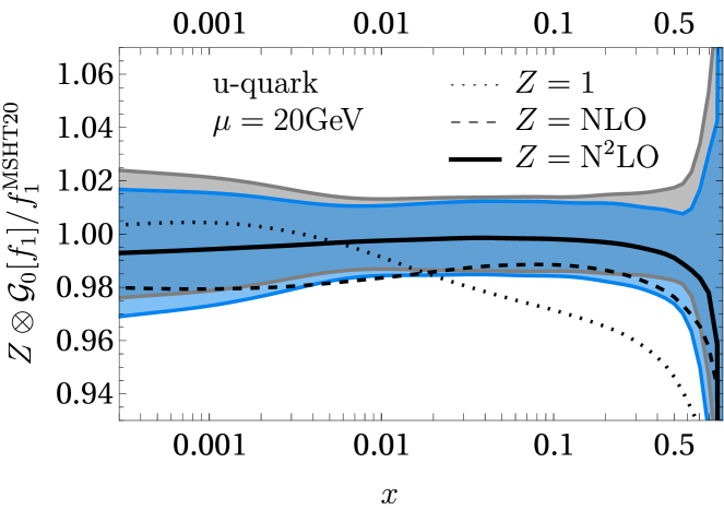
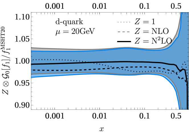
Figure 17: Comparison of the zeroth TMM for TMDPDF with various orders of correcting factor at $\mu=20$ GeV. The comparison is made with the MSHT20 collinear PDF set (gray band). The uncertainty band (blue) is shown only for the N²LO correction factor.

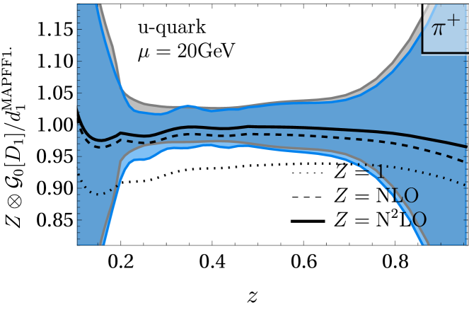
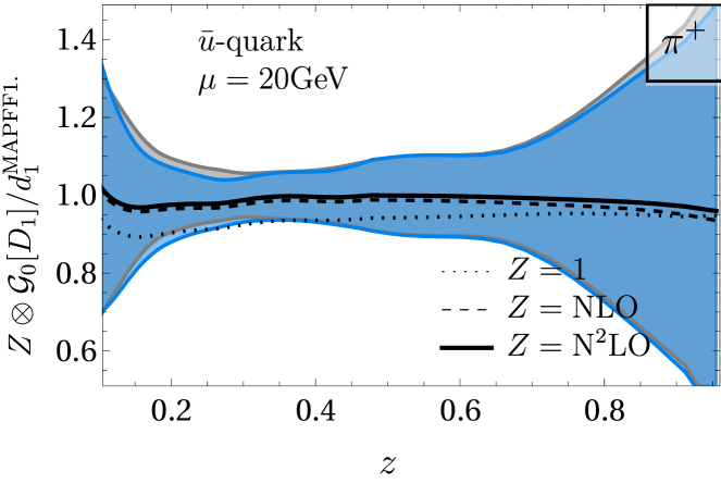
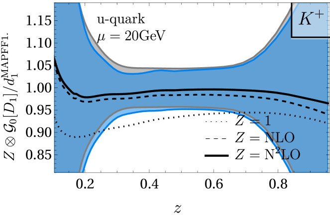
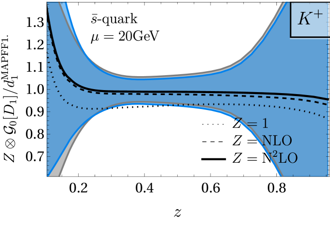
Figure 18: Comparison of the zeroth TMMs for pion (upper row) and kaon (lower row) TMDFFs with various orders of correcting factor at $\mu=20$ GeV. The comparison is made with MAPFF collinear FF (gray band). The uncertainty band (blue) is shown for N²LO correction factor.

The backward determination of collinear FF from TMDFF is depicted in fig. 18 for pion and kaon. The agreement with the MAPFF distributions is also very good. Both the uncertainty band and the mean value are computed independently, without making reference to a particular replica of the FFs. Therefore, the deviation from the input distribution is a bit larger for the regions with larger uncertainties. Also, we would like to emphasize that, despite some TMDFFs behaving strangely (becoming too small, large, or even negative) in particular kinematic regions, the collinear FFs are consistently restored for each one of them.

5.8 The second TMM

The second TMM for the TMD distribution $F$ is defined as delRio:2024vvq

$$\mathcal{M}_{\mu\nu}^{[F]}(x,\mu)=\int^{\mu}d^{2}\bm{k}_{T}\bm{k}_{T\mu}\bm{k}_{T\nu}F(x,\bm{k}_{T}).$$ (52)

It is straightforward to show that this integral is related to the matrix element with two derivatives

$$\mathcal{M}_{\mu\nu}^{[f_{1}]}(x,\mu) = \int\frac{dz}{2\pi}e^{-ixzp^{+}}\langle p|\bar{q}(zn)\mathcal{W}_{\infty}^{\dagger}i\overleftarrow{D}_{\mu}i\overleftarrow{D}_{\nu}\frac{\gamma^{+}}{2}\mathcal{W}_{\infty}q(0)|p\rangle+\mathcal{O}(\mu^{-2}),$$ (53)

where $\mathcal{W}$ is a half-infinite Wilson line in the direction $n$, and $D$ is the covariant derivative. The TMM in eq. (53) refers to unpolarized TMDPDF. The TMM for unpolarized TMDFF is given by an analogous formula.

Similarly, to the zeroth TMM eq. (51), the integration limit $\mu$ is required to cut-off the ultraviolet divergence, which is quadratic for operator eq. (53). The quadratic ultraviolet divergence of operator (and consequently quadratic scaling) is correct in the physical renormalizaton scheme. However, it is absent in the $\overline{\text{MS}}$-scheme, where one discard power divergences. In order to match the integral to $\overline{\text{MS}}$ scheme one has to subtract this divergent part, which can be computed independently, and expresses via convolution of perturbative factor with collinear distribution. The perturbative part of the subtraction term is known to N³LO. For details on the definitions, we refer to the original work delRio:2024vvq .

Altogether, this procedure allows one to consistently define the second TMM, $\mathcal{M}_{\mu\nu}$, in an $\overline{\text{MS}}$-like scheme. The finite scheme-dependent parts of the scheme could not be matched, due to missed expressions for twist-four operators. The matrix element $\mathcal{M}_{\mu\nu}$ has a naive interpretation as the measurement of $\bm{k}_{\mu}\bm{k}_{\nu}$ within the hadron (in the light-cone gauge). In this naive approximation, one can also define the average momentum squared $\langle\bm{k}_{T}^{2}\rangle$ delRio:2024vvq , which reads

$$\langle\bm{k}_{T}^{2}\rangle(x,\mu) = \int^{\mu}d^{2}\bm{k}_{T}\bm{k}_{T}^{2}F(x,\bm{k}_{T})-\mu^{2}\text{AS}[F](x,\mu).$$ (54)

Here, $\text{AS}[F]$ is the coefficient of the power divergency, which we compute at N³LO.

The values of $\langle\bm{k}_{T}^{2}\rangle$ for unpolarized TMDPDF are shown in fig. 19. This quantity grows at smaller $x$, as one would expect naively. All distributions, apart of $\bar{u}$, demonstrate reasonable behavior. Meanwhile, the $\bar{u}$ quark has a rather uncommon shape of $\langle\bm{k}_{T}^{2}\rangle$. It presents a peak at $x\sim 0.1$ with large uncertainties. In this region we do not have sensitivity to anti-quark distribution, and most probably this behavior is an artifact of missing precision and/or shortcomings of the elements in the fit. Since the source of this misbehavior is unclear, and it does not affect the description of the data, we leave the treatment of this problem for future works.

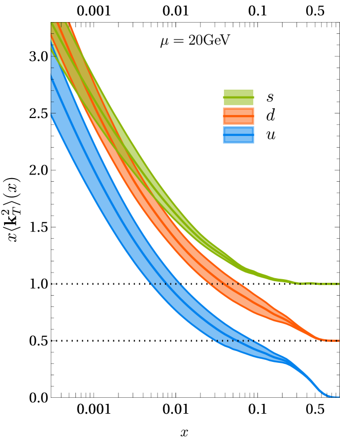
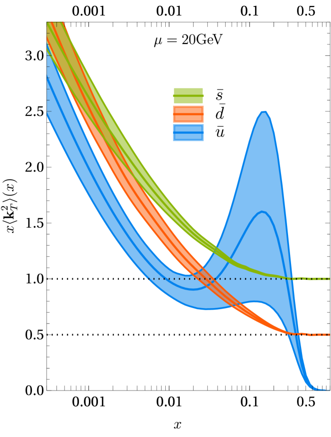
Figure 19: The average momentum-squared determined from the unpolarized TMDPDF for different parton flavors as a function of $x$. For better visibility some distributions are shifted by constant off-set, indicated by the dotted lines.

The integral over $x$ for $\langle\bm{k}_{T}^{2}\rangle$ is divergent. However, the valence combination should produce a finite result. Defining

$$\langle\bm{k}_{T}^{2}\rangle_{q-\text{val.}}(\mu)=\int_{0}^{1}dx\left[\langle\bm{k}_{T}^{2}\rangle_{q}(x,\mu)-\langle\bm{k}_{T}^{2}\rangle_{\bar{q}}(x,\mu)\right],$$ (55)

we find (at $\mu=20$ GeV)

$$\langle\bm{k}_{T}^{2}\rangle_{d-\text{val.}}=1.0^{+0.4}_{-0.5}\text{ GeV}^{2},\qquad\langle\bm{k}_{T}^{2}\rangle_{u-\text{val.}}=-4.7^{+3.4}_{-3.5}\text{ GeV}^{2}.$$ (56)

In order to calculate this number, we computed the integral with the lower limit $x=10^{-4}$ and extrapolated the result down to $x=0$. The difference between the finite integral and the extrapolation is $\sim$ 3-4$\%$. The $\langle\bm{k}_{T}^{2}\rangle$ for u-valence quark is negative due to the large contribution of the $\bar{u}$ term. If we interpolate the $\bar{u}$ contribution between $10^{-2}$ and $1$ (i.e. ignoring the peak) we get $\langle\bm{k}_{T}^{2}\rangle_{u-\text{val.}}\sim 0.95\text{ GeV}^{2}$.

Additionally we can compute the integral

$$\langle x\bm{k}_{T}^{2}\rangle(\mu)=\int_{0}^{1}dxx\langle\bm{k}_{T}^{2}\rangle_{q}(x,\mu),$$ (57)

which is finite. We obtain the following values (at $\mu=20$ GeV)

$$\langle x\bm{k}_{T}^{2}\rangle_{d}=0.44_{-0.07}^{+0.07}, \langle x\bm{k}_{T}^{2}\rangle_{u}=0.66_{-0.06}^{+0.06}, \langle x\bm{k}_{T}^{2}\rangle_{s}=0.15_{-0.02}^{+0.02},$$ (58)

$$\langle x\bm{k}_{T}^{2}\rangle_{\bar{d}}=0.25_{-0.03}^{+0.03}, \langle x\bm{k}_{T}^{2}\rangle_{\bar{u}}=1.93_{-0.81}^{+0.85}, \langle x\bm{k}_{T}^{2}\rangle_{\bar{s}}=0.14_{-0.01}^{+0.02}.$$

The peculiar excess of $\bar{u}$ quark is very transparent here.

The corresponding plots for $\langle\bm{k}_{T}^{2}\rangle$ within unpolarized TMDFFs are shown in fig. 20 for pion and in fig. 21 for kaon. The obvious feature is that this matrix element grows much faster for TMDFF than for TMDPDF (we multiply the plot by $z^{5}$ to balance this growth). This is also obvious from fig. 14 and 15. Also here some of the distributions are negative, which is the result of $\sim b^{2}$ term in our fitting ansatz. At the present stage we cannot decide if this behavior is physical, a product of our fitting, or the result of the some tensions between theory and the data.

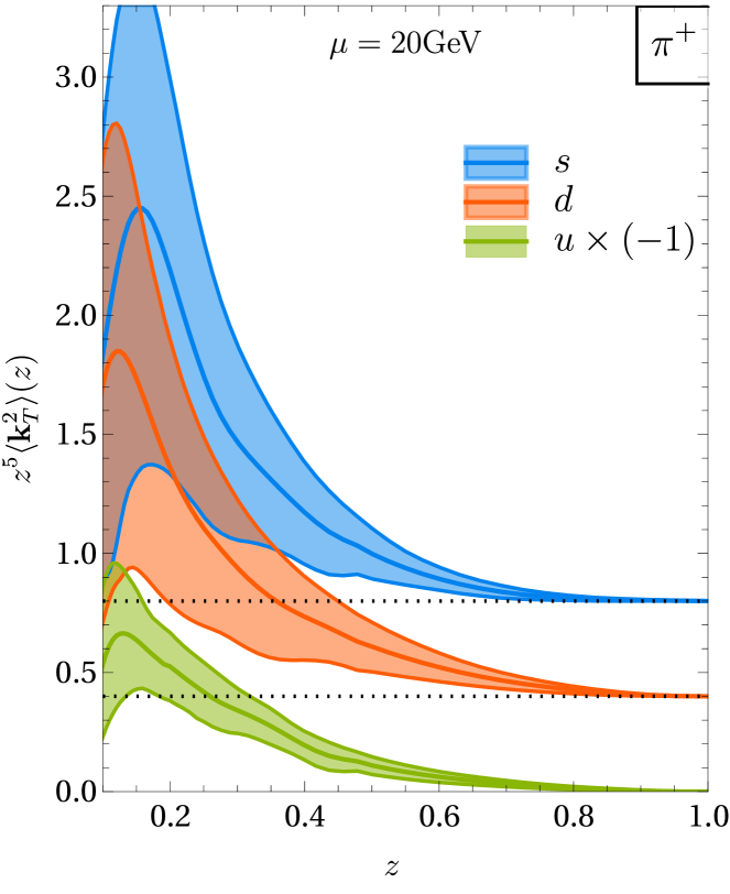
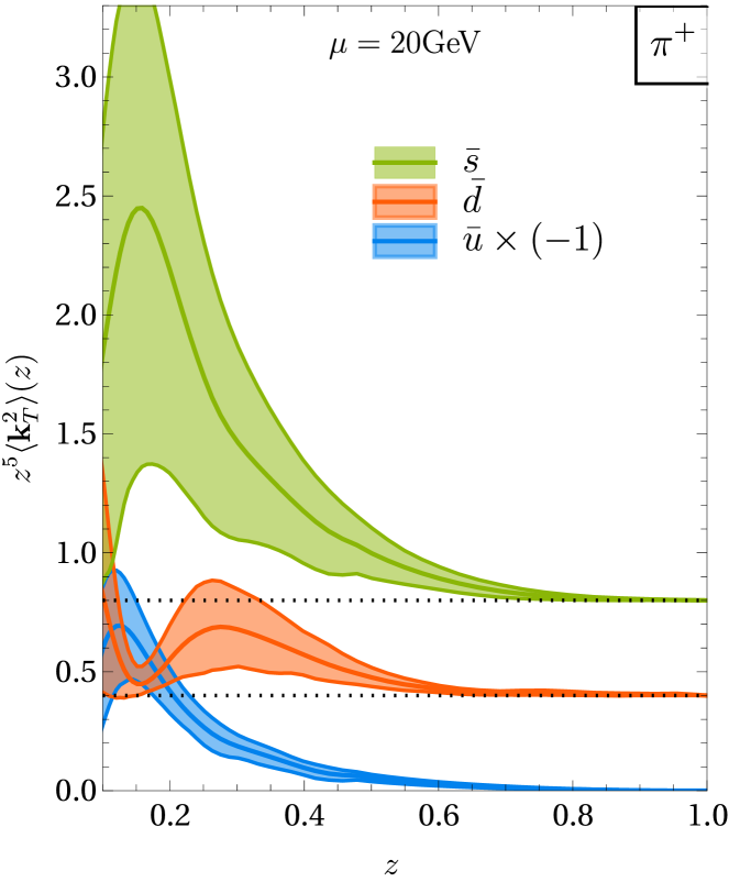
Figure 20: The average momentum-squared determined from the unpolarized TMDFF of pion for different flavors as a function of $z$. For better visibility some flavors are shifted by constant off-set, indicated by dotted lines.

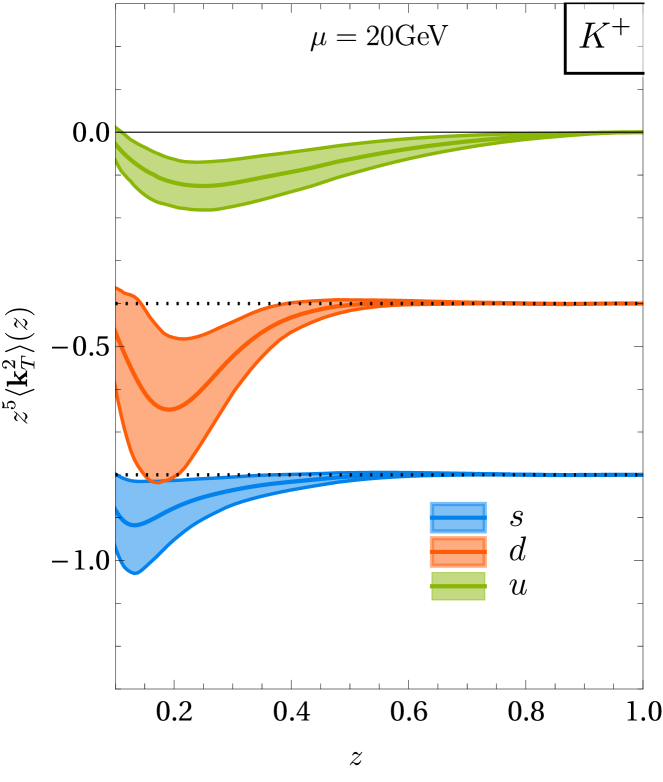
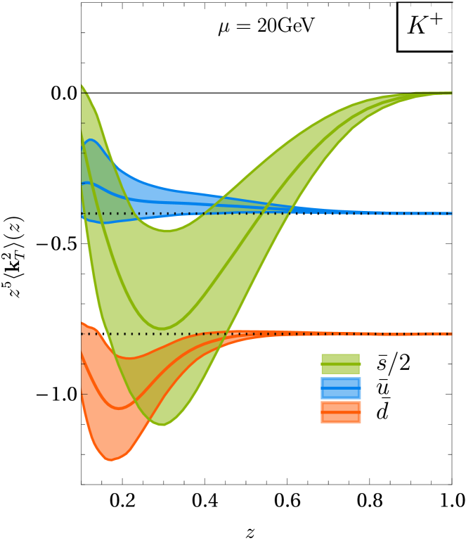
Figure 21: The average momentum-squared determined from the unpolarized TMDFF of kaon for different flavors as a function of $z$. For better visibility some flavors are shifted by constant off-set shown by dotted lines. The $\bar{s}$ distribution is divided by 2 for better visibility.

6 Conclusions

We have performed a global analysis of Drell-Yan and SIDIS data within the framework of the TMD factorization theorem. Compared to the ART23 study Moos:2023yfa , which focused on Drell-Yan data, our analysis additionally includes SIDIS data, allowing us to determine the unpolarized TMDFFs. The main theoretical advancements of this study include the use of N⁴LL perturbative input (for the first time, incorporating large-$x$ resummation), the $\zeta$-prescription, and a flavor-dependent treatment of non-perturbative inputs. We confirm the excellent agreement between the TMD factorization framework (including TMD evolution effects) and SIDIS data, as previously reported in Scimemi:2019cmh . The analysis has been conducted using the artemide code, which is publicly available in the repository artemide .

The present study is supplemented by a detailed discussion of the properties of the extracted TMD distributions in both $b$- and $\bm{k}_{T}$-spaces. In particular, we use transverse momentum moments (TMMs) delRio:2024vvq to verify and quantify various aspects of these distributions. By employing the zeroth TMM, we demonstrate the consistency between the uncertainties of the extracted TMDs and the input collinear distributions, finding a remarkably precise agreement between them. Additionally, using the second TMM, we provide the first-ever estimation of $\langle\bm{k}_{T}^{2}\rangle$ for a parton within the hadron in a model independent way.

Among the various features of this fit, we highlight two notable anomalies: an unusual behavior of the TMDPDF for the $\bar{u}$ flavor (also observed in Moos:2023yfa ) and the exceptionally large size of the TMDFF for $\bar{s}$ in $K^{+}$. We have not identified any specific reasons for these anomalies and attribute them to potential issues in the collinear input.

We present a detailed comparison of our extraction with previous studies. The Collins-Soper (CS) kernel determined in this work is larger than that obtained in previous fits Moos:2023yfa ; Bacchetta:2022awv ; Bacchetta:2024qre . However, it remains consistent with our earlier combined analysis of SIDIS and DY data Scimemi:2019cmh and with the recent neural-network determination Bacchetta:2025ara . This discrepancy suggests a potential model bias in traditional phenomenological extractions of the CS kernel and indicates a systematic underestimation of uncertainties in this quantity. Addressing this issue should be a priority for future studies.

Currently, there is no consensus on whether TMD factorization can adequately describe SIDIS data. While earlier studies Anselmino:2013lza ; Bacchetta:2017gcc did not encounter any issues, the incorporation of TMD evolution into the analysis appears to be problematic. The MAP collaboration reported a significant discrepancy between theoretical predictions and SIDIS data Bacchetta:2022awv ; Bacchetta:2024qre . In contrast, we do not observe any difficulty in describing these data. This disagreement can either arise due to differences in the implementation of the TMD factorization theorem which are vanishing at large $Q$ (and thus formally are the part of power corrections), or be due to restrictions of used non-perturbative models, or derive from unidentified sources. In a future work, we plan to conduct a dedicated investigation to identify the source of this disagreement.

Appendix A Plots of data

In this appendix, we present figures comparing experimental data with theoretical predictions. Due to the large amount of data, collider Drell-Yan measurements are grouped together. Each plot includes significantly more data than used in the fit, allowing us to illustrate the behavior of theoretical predictions beyond the limits of the factorization theorem. Data points included in the fit are shown as filled markers, while those excluded from the fit are displayed as empty markers. For better visualization, the Drell-Yan predictions are uniformly shifted by a percentage indicated in the plots. In some cases, both the cross-section and the predictions are multiplied by a common factor, also specified in the plots, to enhance clarity.

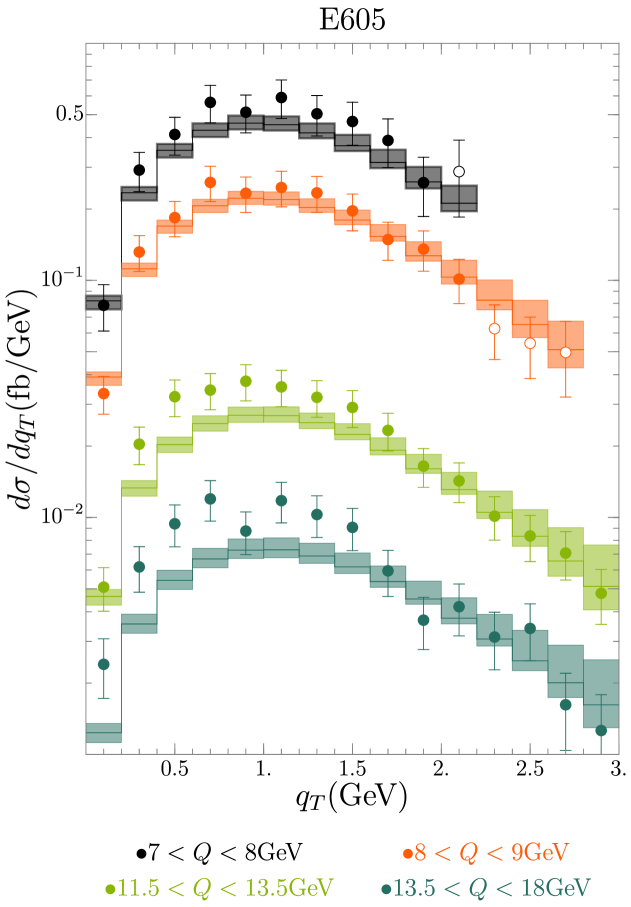
Figure 22: Comparison of ART25 prediction with measurements of Drell-Yan reaction by E605 Moreno:1990sf and E772 E772:1994cpf experiments.

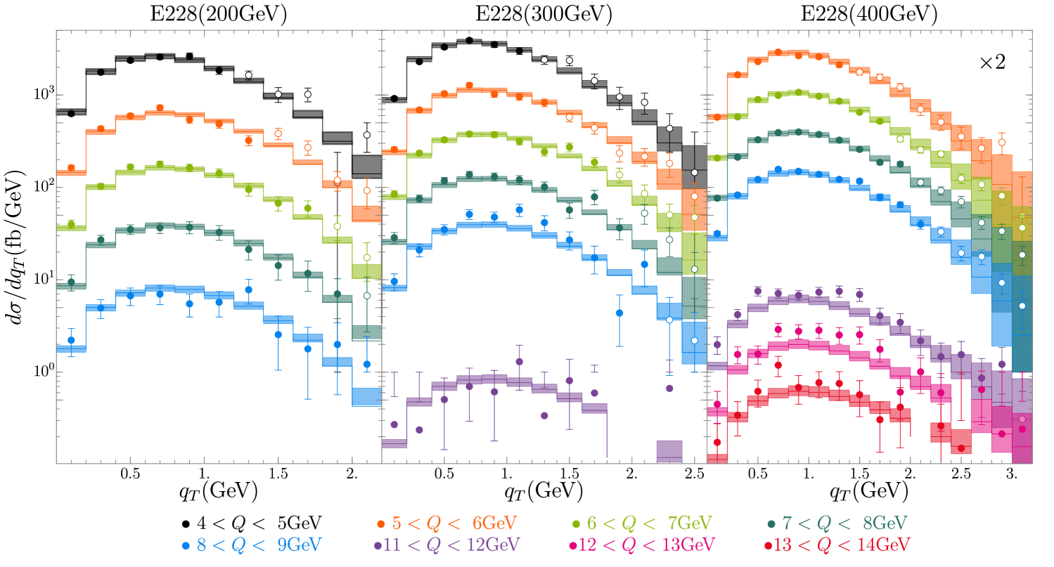
Figure 23: Comparison of ART25 prediction with measurements of Drell-Yan reaction by E228 experiment Ito:1980ev .

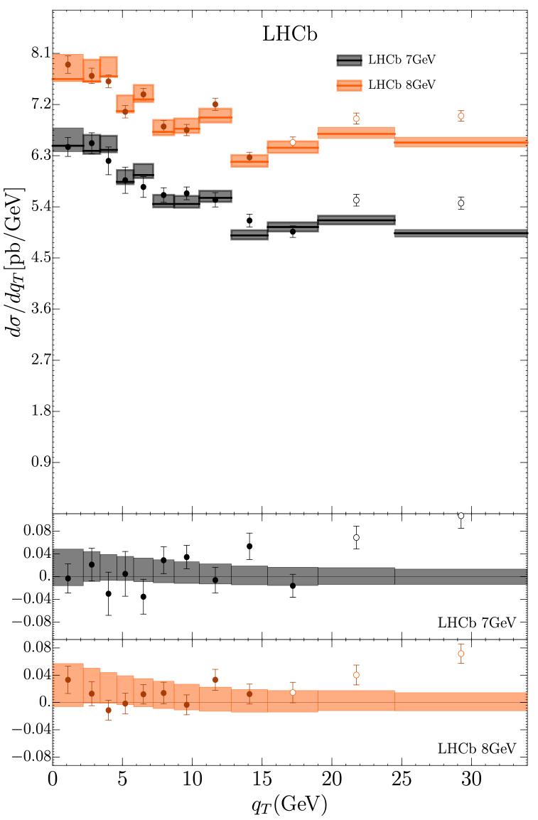
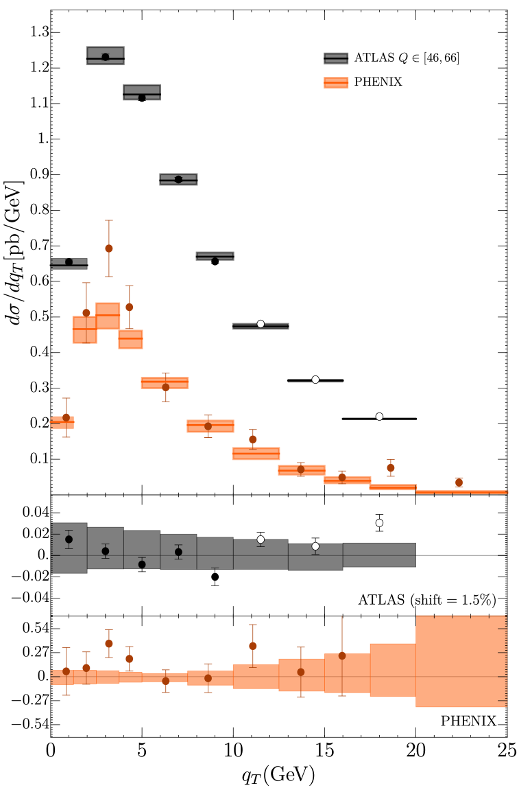
Figure 24: Left panel: comparison of ART25 prediction with measurements of vector boson production above Z-boson peak by LHCb LHCb:2015okr ; LHCb:2015mad . Right panel: comparison of ART25 prediction with measurements of Z-boson production by ATLAS, and PHENIX ATLAS:2019zci ; PHENIX:2018dwt .

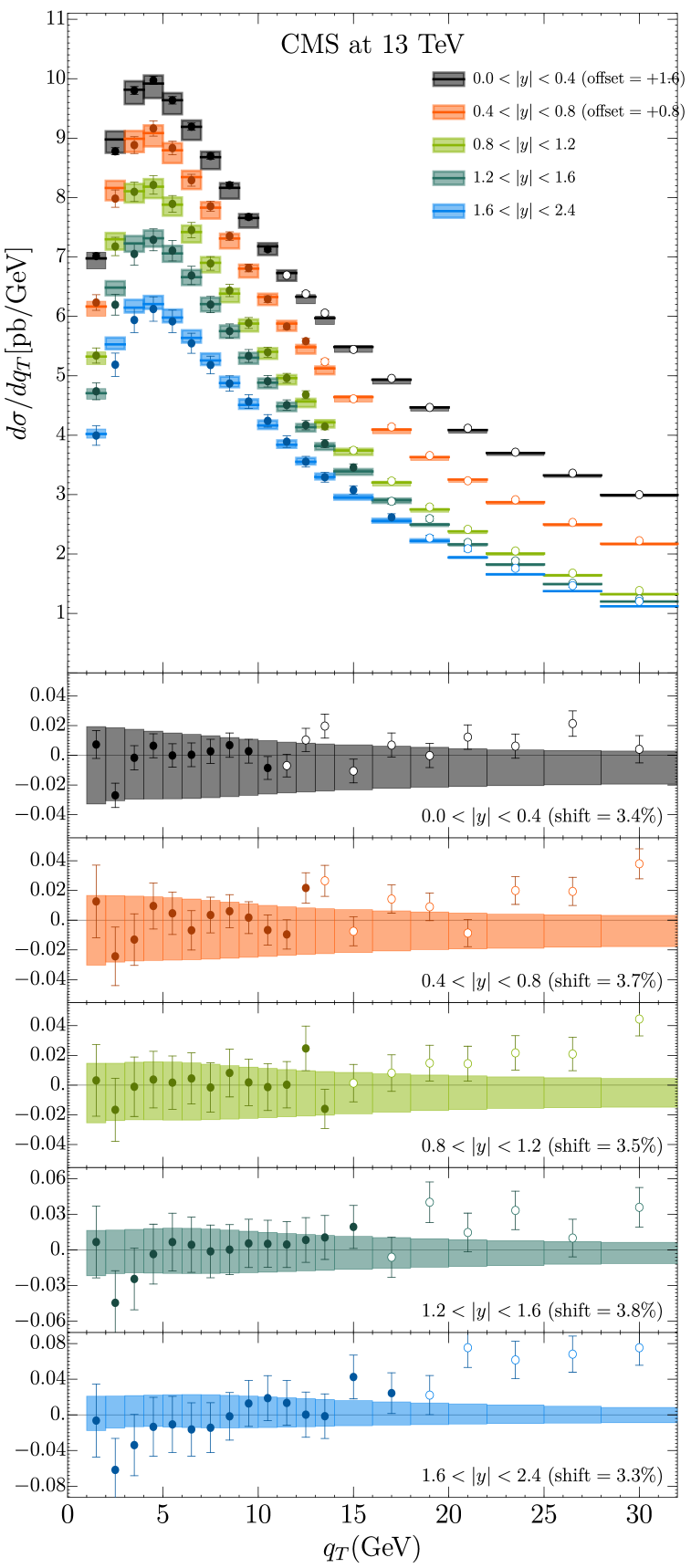
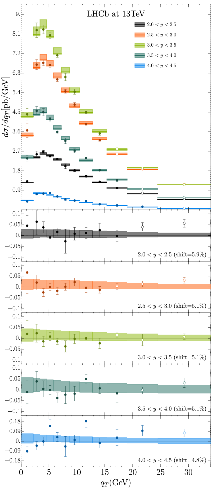
Figure 26: Comparison of ART25 prediction with measurements of Z-boson production at different values of rapidity by CMS CMS:2019raw (left panel) and by LHCb LHCb:2021huf (right panel).

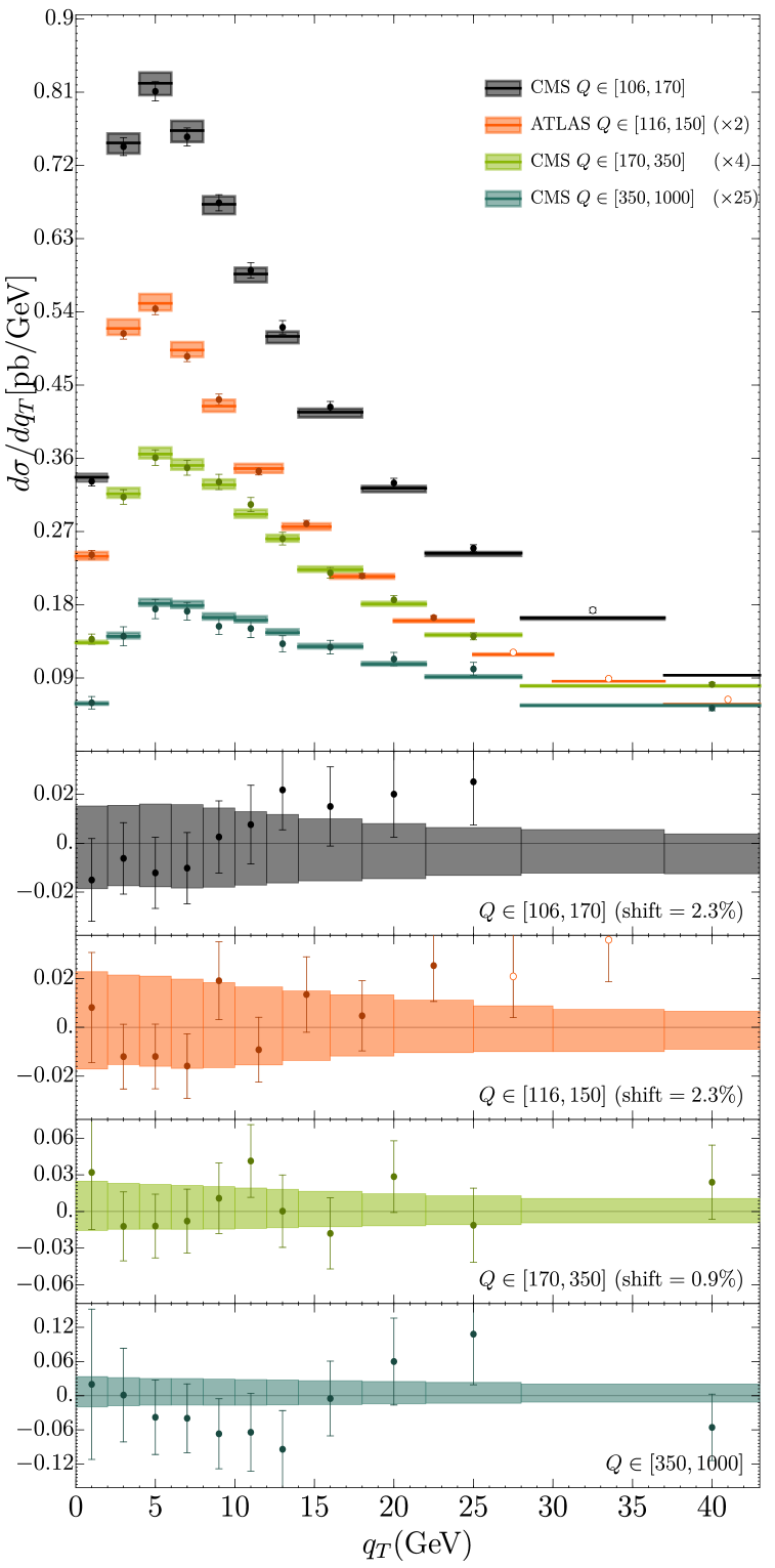
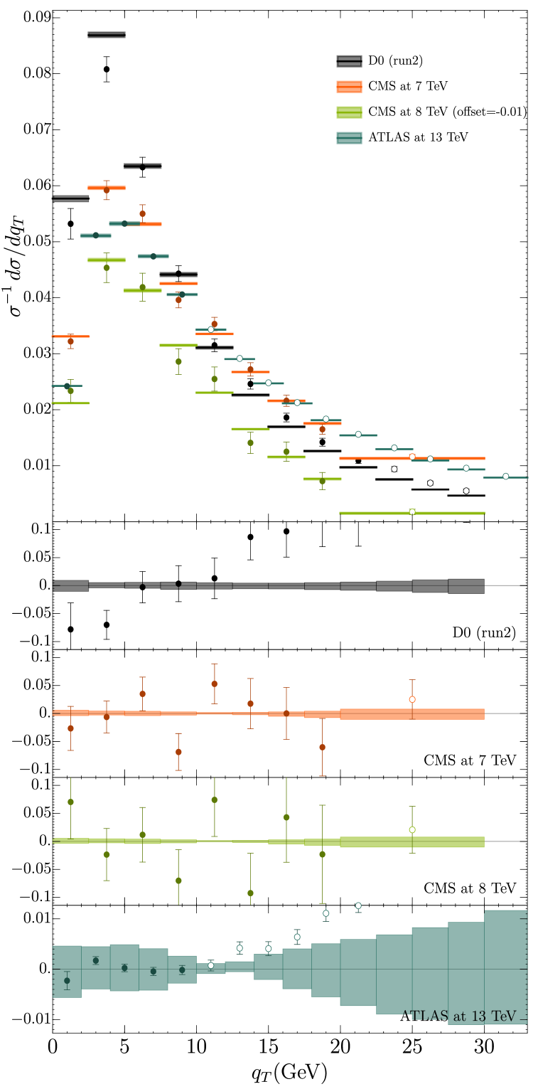
Figure 27: Left panel: comparison of ART25 prediction with measurements of vector boson production above Z-boson peak by ATLAS and CMS ATLAS:2015iiu ; CMS:2022ubq . Right panel: comparison of ART25 prediction with measurements of Z-boson production by ATLAS, CMS and D0 ATLAS:2019zci ; CMS:2011wyd ; CMS:2016mwa ; D0:1999jba normalized to the total cross-section.

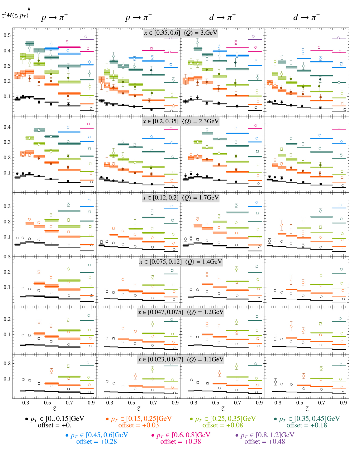
Figure 28: Comparison of ART25 prediction for pion production in SIDIS measured at HERMES HERMES:2012uyd . For better visibility, points with different bins in $p_{T}$ are shifted by a common value indicated in the legend.

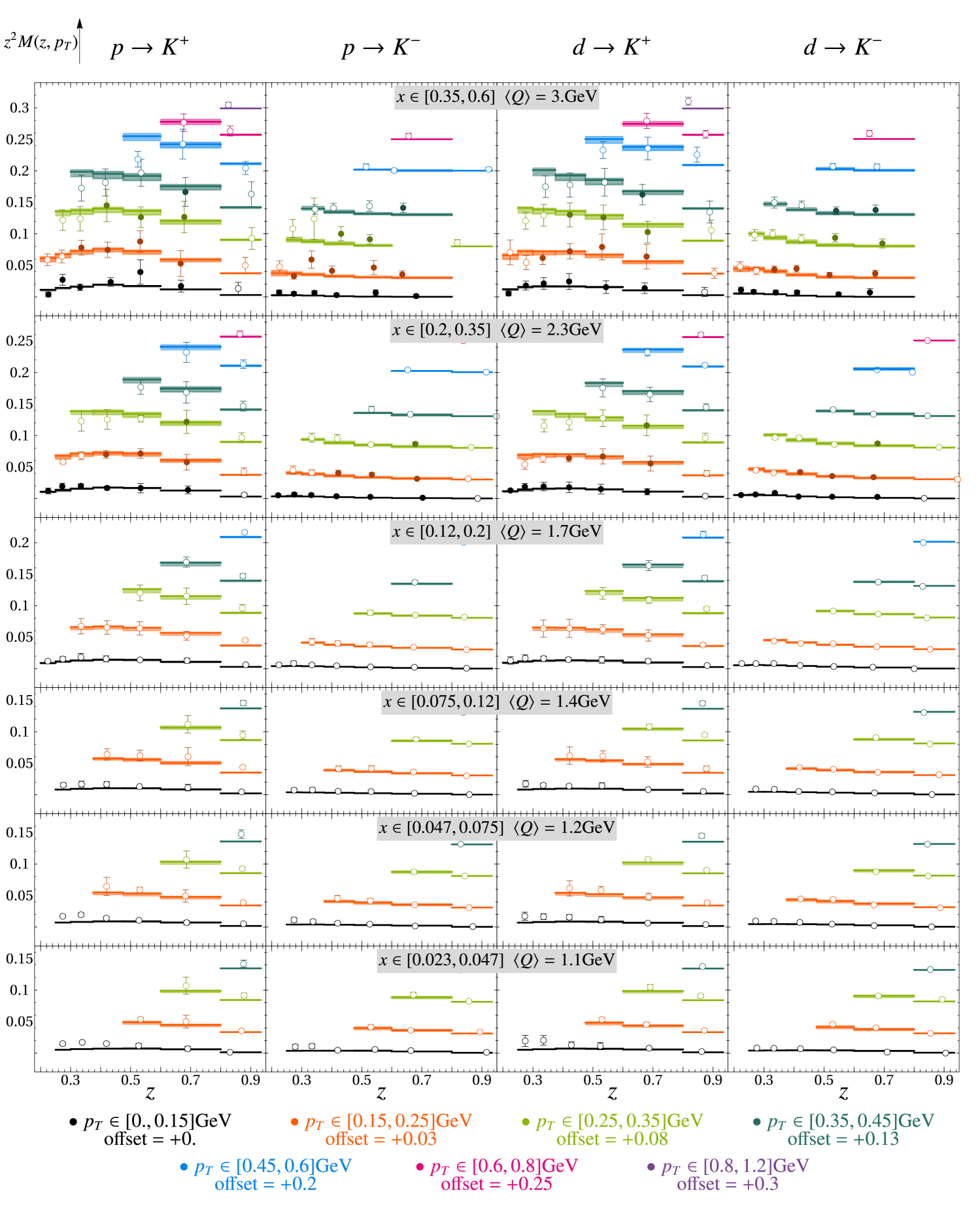
Figure 29: Comparison of ART25 prediction for kaon production in SIDIS measured at HERMES HERMES:2012uyd . For better visibility, points with different bins in $p_{T}$ are shifted by a common value indicated in the legend.

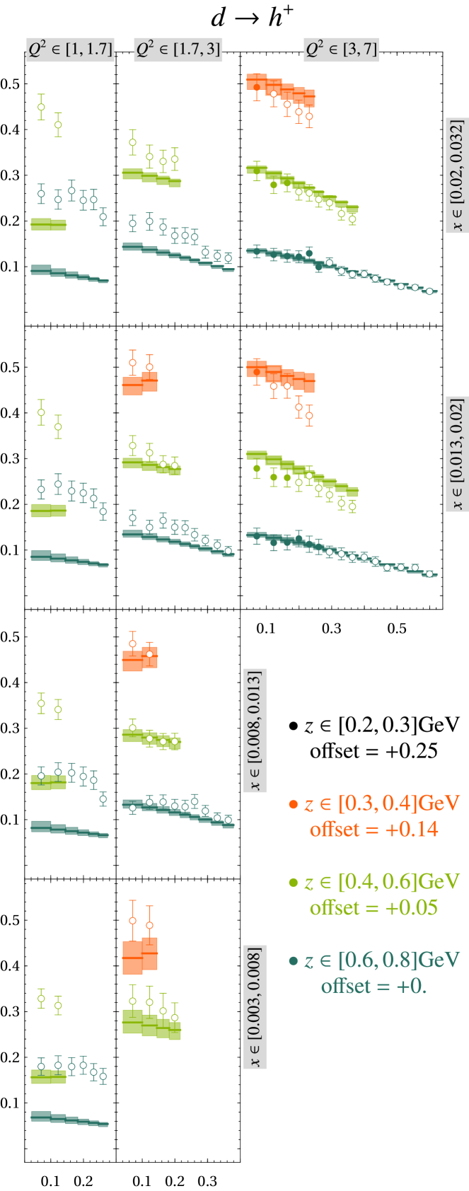
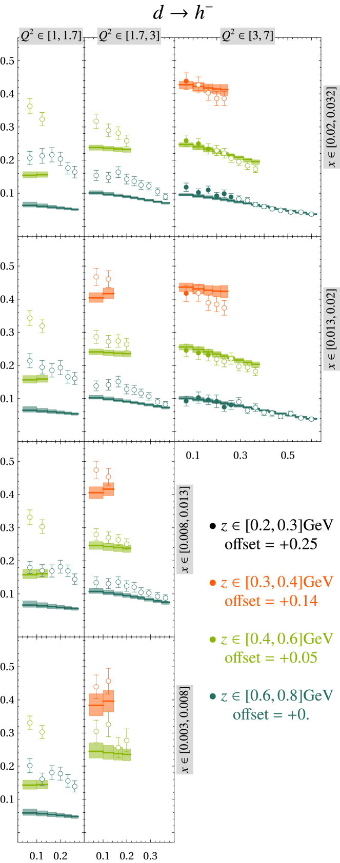
Figure 32: Continuation of figures 30 (left panel) and 31 (right panel).

Appendix B Plots of comparison with different extractions

In this appendix we present plots comparing the present extraction (ART25) with extractions made in refs. Moos:2023yfa (ART23), Bacchetta:2022awv (MAP22), Bacchetta:2024qre (MAP24) and Bacchetta:2025ara (MAPNN). The comparison is made for TMD distributions in $b$ space, because it is the representation in which TMD distributions are extracted from the data. All comparisons are presented for TMD distributions evaluated at 10 GeV, i.e. at scales $\mu=10$ GeV and $\zeta=10^{2}$ GeV².

TMDPDFs are compared at values of $x=0.1$ and $x=0.01$ as typical values that contribute to Drell-Yan and SIDIS data, in the two upper rows of fig. 33 and 34, respectively. Additionally, in the two lower rows of each figure we present the sizes of the uncertainty bands, relative to the central values of the corresponding TMD distributions.

The comparison of pion TMDFFs is presented in fig. 35 at $z=0.3$. The comparison of kaon TMDFFs is presented in fig. 36 at $z=0.3$.

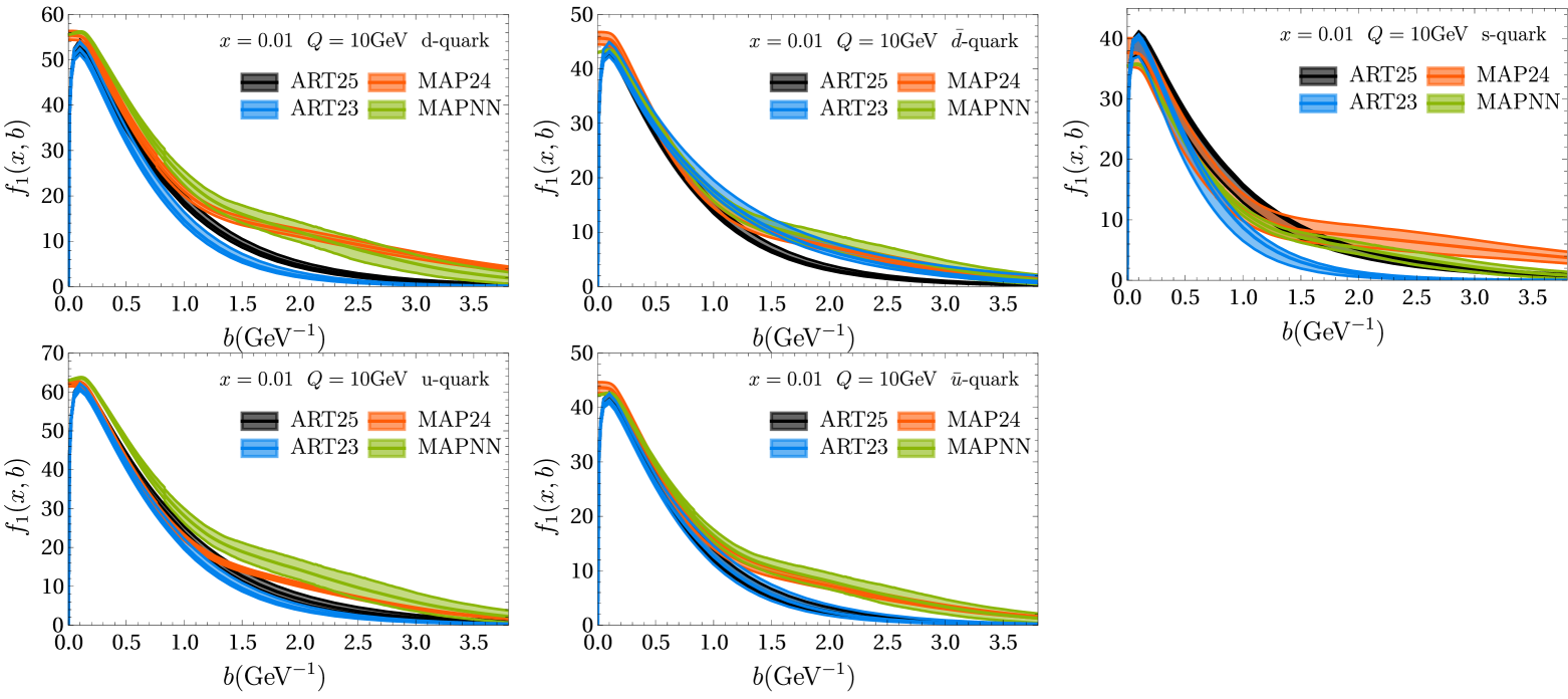
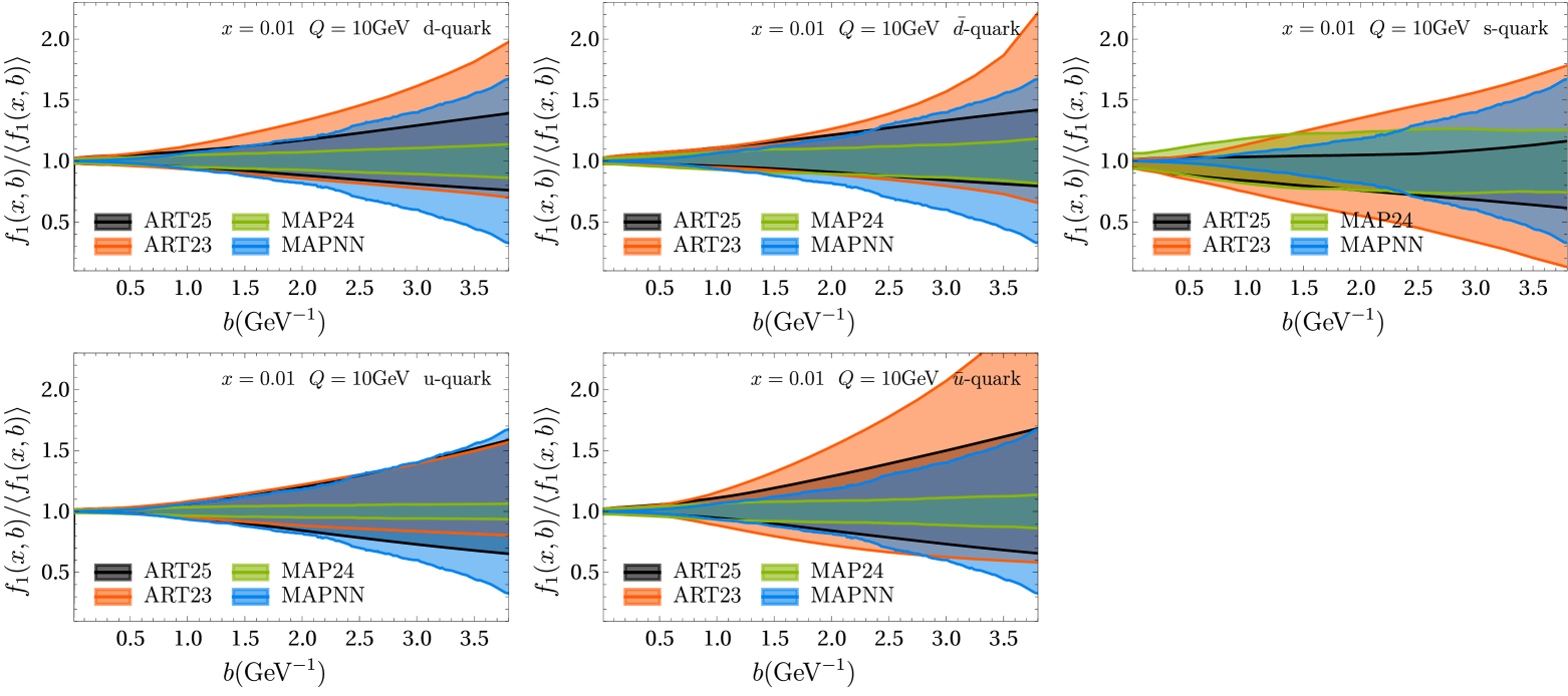
Figure 33: Comparison of uTMDPDFs and sizes of their uncertainty bands as function of $b$ at $x=0.01$ between different extractions.

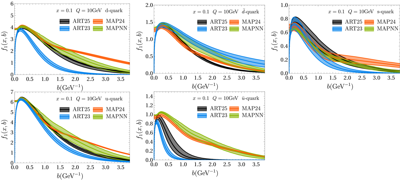
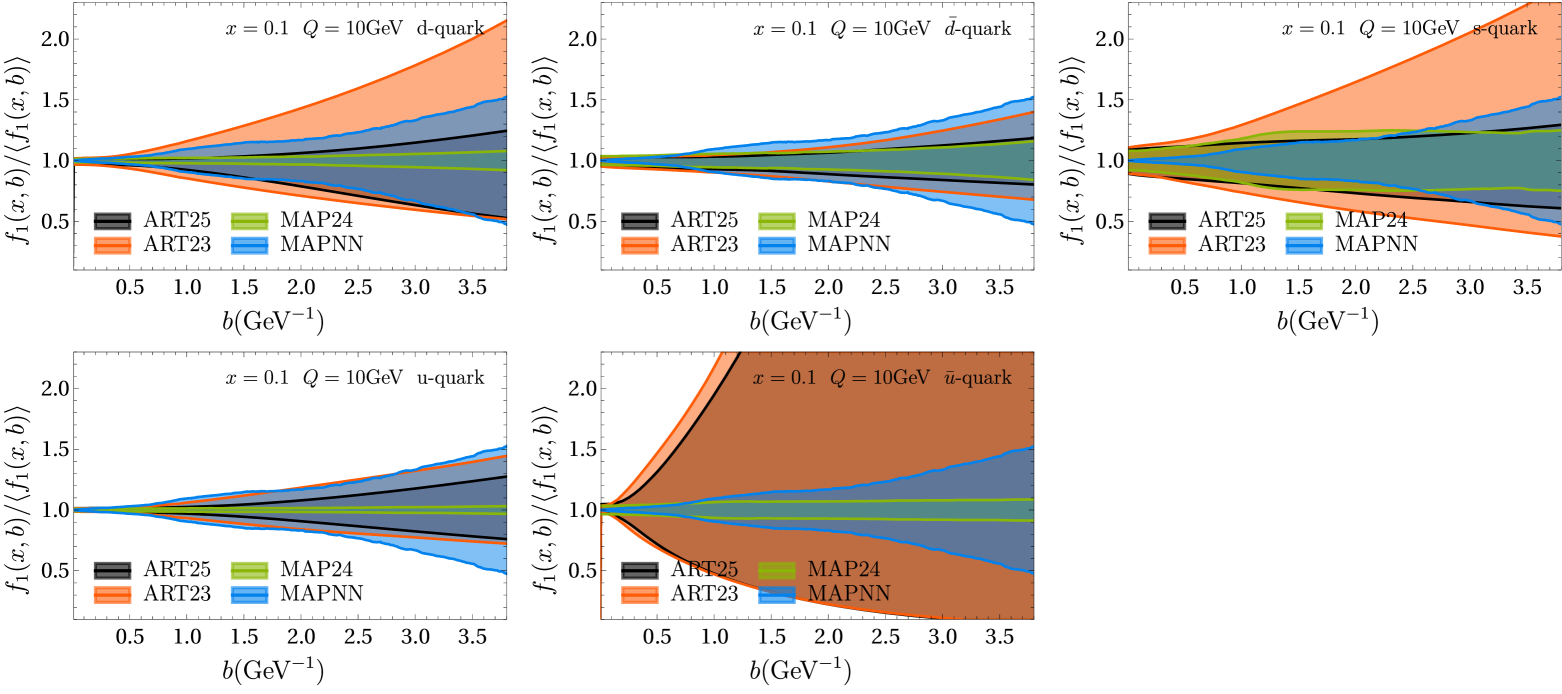
Figure 34: Comparison of uTMDPDFs and sizes of their uncertainty bands as function of $b$ at $x=0.1$ between different extractions.

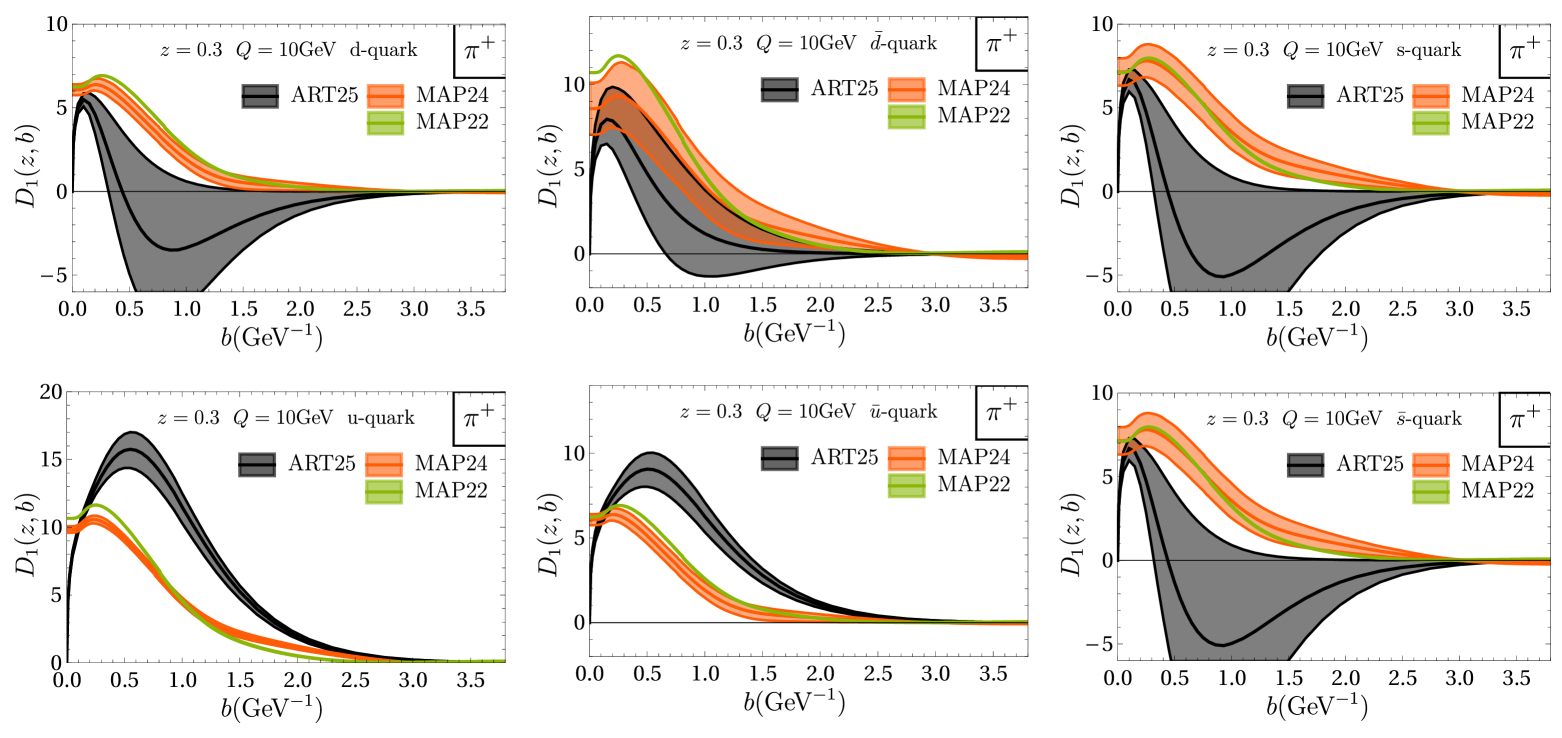
Figure 35: Comparison of TMDFFs for pion as function of $b$ at $z=0.3$ between different extractions.

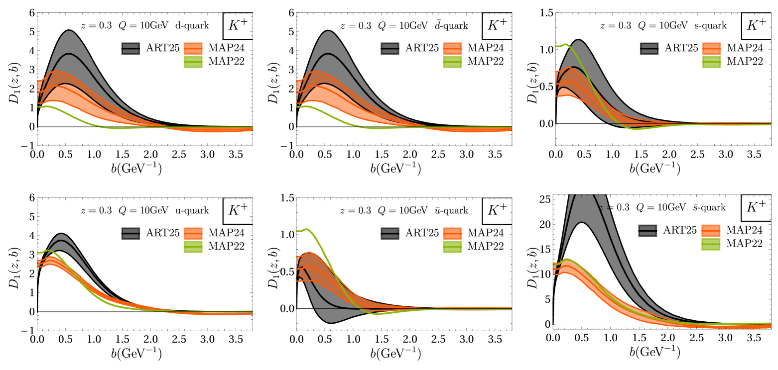
Figure 36: Comparison of TMDFFs for kaon as function of $b$ at $z=0.3$ between different extractions.

References

- (1) J.C. Collins and D.E. Soper, Back-To-Back Jets in QCD, Nucl. Phys. B 193 (1981) 381.
- (2) J.C. Collins and D.E. Soper, Back-To-Back Jets: Fourier Transform from B to K-Transverse, Nucl. Phys. B 197 (1982) 446.
- (3) J.C. Collins, D.E. Soper and G.F. Sterman, Factorization of Hard Processes in QCD, Adv. Ser. Direct. High Energy Phys. 5 (1989) 1 [hep-ph/0409313].
- (4) J. Collins, Foundations of perturbative QCD, vol. 32, Cambridge University Press (11, 2013).
- (5) T. Becher and M. Neubert, Drell-Yan Production at Small , Transverse Parton Distributions and the Collinear Anomaly, Eur. Phys. J. C 71 (2011) 1665 [1007.4005].
- (6) M.G. Echevarria, A. Idilbi and I. Scimemi, Factorization Theorem For Drell-Yan At Low And Transverse Momentum Distributions On-The-Light-Cone, JHEP 07 (2012) 002 [1111.4996].
- (7) J.-Y. Chiu, A. Jain, D. Neill and I.Z. Rothstein, A Formalism for the Systematic Treatment of Rapidity Logarithms in Quantum Field Theory, JHEP 05 (2012) 084 [1202.0814].
- (8) A. Vladimirov, V. Moos and I. Scimemi, Transverse momentum dependent operator expansion at next-to-leading power, JHEP 01 (2022) 110 [2109.09771].
- (9) A. Bacchetta, F. Delcarro, C. Pisano, M. Radici and A. Signori, Extraction of partonic transverse momentum distributions from semi-inclusive deep-inelastic scattering, Drell-Yan and Z-boson production, JHEP 06 (2017) 081 [1703.10157].
- (10) I. Scimemi and A. Vladimirov, Non-perturbative structure of semi-inclusive deep-inelastic and Drell-Yan scattering at small transverse momentum, JHEP 06 (2020) 137 [1912.06532].
- (11) MAP (Multi-dimensional Analyses of Partonic distributions) collaboration, Unpolarized transverse momentum distributions from a global fit of Drell-Yan and semi-inclusive deep-inelastic scattering data, JHEP 10 (2022) 127 [2206.07598].
- (12) MAP collaboration, Flavor dependence of unpolarized quark transverse momentum distributions from a global fit, JHEP 08 (2024) 232 [2405.13833].
- (13) A. Vladimirov, “artemide v3.01.” https://github.com/VladimirovAlexey/artemide-public. https://doi.org/10.5281/zenodo.15006449.
- (14) I. Scimemi and A. Vladimirov, Analysis of vector boson production within TMD factorization, Eur. Phys. J. C 78 (2018) 89 [1706.01473].
- (15) V. Bertone, I. Scimemi and A. Vladimirov, Extraction of unpolarized quark transverse momentum dependent parton distributions from Drell-Yan/Z-boson production, JHEP 06 (2019) 028 [1902.08474].
- (16) A. Vladimirov, Pion-induced Drell-Yan processes within TMD factorization, JHEP 10 (2019) 090 [1907.10356].
- (17) M. Bury, A. Prokudin and A. Vladimirov, Extraction of the Sivers Function from SIDIS, Drell-Yan, and Data at Next-to-Next-to-Next-to Leading Order, Phys. Rev. Lett. 126 (2021) 112002 [2012.05135].
- (18) M. Bury, A. Prokudin and A. Vladimirov, Extraction of the Sivers function from SIDIS, Drell-Yan, and boson production data with TMD evolution, JHEP 05 (2021) 151 [2103.03270].
- (19) M. Bury, F. Hautmann, S. Leal-Gomez, I. Scimemi, A. Vladimirov and P. Zurita, PDF bias and flavor dependence in TMD distributions, JHEP 10 (2022) 118 [2201.07114].
- (20) M. Horstmann, A. Schafer and A. Vladimirov, Study of the worm-gear-T function g1T with semi-inclusive DIS data, Phys. Rev. D 107 (2023) 034016 [2210.07268].
- (21) V. Moos, I. Scimemi, A. Vladimirov and P. Zurita, Extraction of unpolarized transverse momentum distributions from the fit of Drell-Yan data at N4LL, JHEP 05 (2024) 036 [2305.07473].
- (22) A. Bacchetta, V. Bertone, C. Bissolotti, G. Bozzi, F. Delcarro, F. Piacenza et al., Transverse-momentum-dependent parton distributions up to N3LL from Drell-Yan data, JHEP 07 (2020) 117 [1912.07550].
- (23) O. del Rio, A. Prokudin, I. Scimemi and A. Vladimirov, Transverse momentum distributions at large-, 2501.17274.
- (24) O. del Rio, A. Prokudin, I. Scimemi and A. Vladimirov, Transverse momentum moments, Phys. Rev. D 110 (2024) 016003 [2402.01836].
- (25) I. Scimemi and A. Vladimirov, Systematic analysis of double-scale evolution, JHEP 08 (2018) 003 [1803.11089].
- (26) Particle Data Group collaboration, Review of Particle Physics, PTEP 2022 (2022) 083C01.
- (27) S. Bailey, T. Cridge, L.A. Harland-Lang, A.D. Martin and R.S. Thorne, Parton distributions from LHC, HERA, Tevatron and fixed target data: MSHT20 PDFs, Eur. Phys. J. C 81 (2021) 341 [2012.04684].
- (28) R.N. Lee, A. von Manteuffel, R.M. Schabinger, A.V. Smirnov, V.A. Smirnov and M. Steinhauser, Quark and Gluon Form Factors in Four-Loop QCD, Phys. Rev. Lett. 128 (2022) 212002 [2202.04660].
- (29) S. Moch, B. Ruijl, T. Ueda, J.A.M. Vermaseren and A. Vogt, On quartic colour factors in splitting functions and the gluon cusp anomalous dimension, Phys. Lett. B 782 (2018) 627 [1805.09638].
- (30) F. Herzog, S. Moch, B. Ruijl, T. Ueda, J.A.M. Vermaseren and A. Vogt, Five-loop contributions to low-N non-singlet anomalous dimensions in QCD, Phys. Lett. B 790 (2019) 436 [1812.11818].
- (31) I. Moult, H.X. Zhu and Y.J. Zhu, The four loop QCD rapidity anomalous dimension, JHEP 08 (2022) 280 [2205.02249].
- (32) C. Duhr, B. Mistlberger and G. Vita, Four-Loop Rapidity Anomalous Dimension and Event Shapes to Fourth Logarithmic Order, Phys. Rev. Lett. 129 (2022) 162001 [2205.02242].
- (33) M.-x. Luo, T.-Z. Yang, H.X. Zhu and Y.J. Zhu, Quark Transverse Parton Distribution at the Next-to-Next-to-Next-to-Leading Order, Phys. Rev. Lett. 124 (2020) 092001 [1912.05778].
- (34) M.-X. Luo, X. Wang, X. Xu, L.L. Yang, T.-Z. Yang and H.X. Zhu, Transverse Parton Distribution and Fragmentation Functions at NNLO: the Quark Case, JHEP 10 (2019) 083 [1908.03831].
- (35) M.A. Ebert, B. Mistlberger and G. Vita, TMD Fragmentation Functions at N3LO, JHEP 07 (2021) 121 [2012.07853].
- (36) M.A. Ebert, B. Mistlberger and G. Vita, Transverse momentum dependent PDFs at N3LO, JHEP 09 (2020) 146 [2006.05329].
- (37) MAP (Multi-dimensional Analyses of Partonic distributions) collaboration, Determination of unpolarized pion fragmentation functions using semi-inclusive deep-inelastic-scattering data, Phys. Rev. D 104 (2021) 034007 [2105.08725].
- (38) MAP (Multi-dimensional Analyses of Partonic distributions) collaboration, Pion and kaon fragmentation functions at next-to-next-to-leading order, Phys. Lett. B 834 (2022) 137456 [2204.10331].
- (39) S.M. Aybat and T.C. Rogers, TMD Parton Distribution and Fragmentation Functions with QCD Evolution, Phys. Rev. D 83 (2011) 114042 [1101.5057].
- (40) S. Piloneta and A. Vladimirov, Angular distributions of Drell-Yan leptons in the TMD factorization approach, JHEP 12 (2024) 059 [2407.06277].
- (41) A. Vladimirov, Kinematic power corrections in TMD factorization theorem, JHEP 12 (2023) 008 [2307.13054].
- (42) A. Bacchetta, M. Diehl, K. Goeke, A. Metz, P.J. Mulders and M. Schlegel, Semi-inclusive deep inelastic scattering at small transverse momentum, JHEP 02 (2007) 093 [hep-ph/0611265].
- (43) A.A. Vladimirov, Self-contained definition of the Collins-Soper kernel, Phys. Rev. Lett. 125 (2020) 192002 [2003.02288].
- (44) M.G. Echevarria, I. Scimemi and A. Vladimirov, Universal transverse momentum dependent soft function at NNLO, Phys. Rev. D 93 (2016) 054004 [1511.05590].
- (45) Y. Li and H.X. Zhu, Bootstrapping Rapidity Anomalous Dimensions for Transverse-Momentum Resummation, Phys. Rev. Lett. 118 (2017) 022004 [1604.01404].
- (46) A.A. Vladimirov, Correspondence between Soft and Rapidity Anomalous Dimensions, Phys. Rev. Lett. 118 (2017) 062001 [1610.05791].
- (47) G.P. Korchemsky and G.F. Sterman, Nonperturbative corrections in resummed cross-sections, Nucl. Phys. B 437 (1995) 415 [hep-ph/9411211].
- (48) I. Scimemi and A. Vladimirov, Power corrections and renormalons in Transverse Momentum Distributions, JHEP 03 (2017) 002 [1609.06047].
- (49) HERMES collaboration, Multiplicities of charged pions and kaons from semi-inclusive deep-inelastic scattering by the proton and the deuteron, Phys. Rev. D 87 (2013) 074029 [1212.5407].
- (50) COMPASS collaboration, Transverse-momentum-dependent Multiplicities of Charged Hadrons in Muon-Deuteron Deep Inelastic Scattering, Phys. Rev. D 97 (2018) 032006 [1709.07374].
- (51) ZEUS collaboration, Inclusive charged particle distributions in deep inelastic scattering events at HERA, Z. Phys. C 70 (1996) 1 [hep-ex/9511010].
- (52) H1 collaboration, Measurement of charged particle transverse momentum spectra in deep inelastic scattering, Nucl. Phys. B 485 (1997) 3 [hep-ex/9610006].
- (53) R. Asaturyan et al., Semi-Inclusive Charged-Pion Electroproduction off Protons and Deuterons: Cross Sections, Ratios and Access to the Quark-Parton Model at Low Energies, Phys. Rev. C 85 (2012) 015202 [1103.1649].
- (54) L.A. Harland-Lang, A.D. Martin, P. Motylinski and R.S. Thorne, Parton distributions in the LHC era: MMHT 2014 PDFs, Eur. Phys. J. C 75 (2015) 204 [1412.3989].
- (55) MMHT collaboration, “MMHT 2014 PDFs : stand-alone code.” https://www.hep.ucl.ac.uk/mmht/code.shtml, 2014.
- (56) A.S. Ito et al., Measurement of the Continuum of Dimuons Produced in High-Energy Proton - Nucleus Collisions, Phys. Rev. D 23 (1981) 604.
- (57) G. Moreno et al., Dimuon production in proton - copper collisions at = 38.8-GeV, Phys. Rev. D 43 (1991) 2815.
- (58) E772 collaboration, Cross-sections for the production of high mass muon pairs from 800-GeV proton bombardment of H-2, Phys. Rev. D 50 (1994) 3038.
- (59) PHENIX collaboration, Measurements of pairs from open heavy flavor and Drell-Yan in collisions at GeV, Phys. Rev. D 99 (2019) 072003 [1805.02448].
- (60) STAR collaboration, Measurements of the cross section and transverse single spin asymmetry in 510 GeV collisions, Phys. Lett. B 854 (2024) 138715 [2308.15496].
- (61) CDF collaboration, The transverse momentum and total cross section of pairs in the boson region from collisions at TeV, Phys. Rev. Lett. 84 (2000) 845 [hep-ex/0001021].
- (62) CDF collaboration, Transverse momentum cross section of pairs in the -boson region from collisions at TeV, Phys. Rev. D 86 (2012) 052010 [1207.7138].
- (63) D0 collaboration, Measurement of the shape of the boson transverse momentum distribution in events produced at =1.96-TeV, Phys. Rev. Lett. 100 (2008) 102002 [0712.0803].
- (64) D0 collaboration, Measurement of the inclusive differential cross section for bosons as a function of transverse momentum in collisions at TeV, Phys. Rev. D 61 (2000) 032004 [hep-ex/9907009].
- (65) D0 collaboration, Measurement of the Normalized Transverse Momentum Distribution in Collisions at TeV, Phys. Lett. B 693 (2010) 522 [1006.0618].
- (66) ATLAS collaboration, Measurement of the transverse momentum and distributions of Drell–Yan lepton pairs in proton–proton collisions at TeV with the ATLAS detector, Eur. Phys. J. C 76 (2016) 291 [1512.02192].
- (67) ATLAS collaboration, Measurement of the transverse momentum distribution of Drell–Yan lepton pairs in proton–proton collisions at TeV with the ATLAS detector, Eur. Phys. J. C 80 (2020) 616 [1912.02844].
- (68) CMS collaboration, Measurement of the Rapidity and Transverse Momentum Distributions of Bosons in Collisions at TeV, Phys. Rev. D 85 (2012) 032002 [1110.4973].
- (69) CMS collaboration, Measurement of the transverse momentum spectra of weak vector bosons produced in proton-proton collisions at TeV, JHEP 02 (2017) 096 [1606.05864].
- (70) CMS collaboration, Measurements of differential Z boson production cross sections in proton-proton collisions at = 13 TeV, JHEP 12 (2019) 061 [1909.04133].
- (71) CMS collaboration, Measurement of the mass dependence of the transverse momentum of lepton pairs in Drell-Yan production in proton-proton collisions at = 13 TeV, Eur. Phys. J. C 83 (2023) 628 [2205.04897].
- (72) LHCb collaboration, Measurement of the forward boson production cross-section in collisions at TeV, JHEP 08 (2015) 039 [1505.07024].
- (73) LHCb collaboration, Measurement of forward W and Z boson production in collisions at TeV, JHEP 01 (2016) 155 [1511.08039].
- (74) LHCb collaboration, Precision measurement of forward boson production in proton-proton collisions at TeV, JHEP 07 (2022) 026 [2112.07458].
- (75) CDF collaboration, Measurement of the W P(T) distribution in collisions at TeV, Phys. Rev. Lett. 66 (1991) 2951.
- (76) D0 collaboration, Measurement of the shape of the transverse momentum distribution of bosons produced in collisions at TeV, Phys. Rev. Lett. 80 (1998) 5498 [hep-ex/9803003].
- (77) NNPDF collaboration, A Determination of parton distributions with faithful uncertainty estimation, Nucl. Phys. B 809 (2009) 1 [0808.1231].
- (78) R.D. Ball et al., Parton Distribution Benchmarking with LHC Data, JHEP 04 (2013) 125 [1211.5142].
- (79) A. Vladimirov, “artemide-DataProcessor.” https://github.com/VladimirovAlexey/artemide-DataProcessor.
- (80) H. Dembinski and P.O. et al., scikit-hep/iminuit, .
- (81) MAP collaboration, A Neural-Network Extraction of Unpolarised Transverse-Momentum-Dependent Distributions, 2502.04166.
- (82) D. Bollweg, X. Gao, S. Mukherjee and Y. Zhao, Nonperturbative Collins-Soper kernel from chiral quarks with physical masses, Phys. Lett. B 852 (2024) 138617 [2403.00664].
- (83) A. Avkhadiev, P.E. Shanahan, M.L. Wagman and Y. Zhao, Collins-Soper kernel from lattice QCD at the physical pion mass, Phys. Rev. D 108 (2023) 114505 [2307.12359].
- (84) A. Avkhadiev, P.E. Shanahan, M.L. Wagman and Y. Zhao, Determination of the Collins-Soper Kernel from Lattice QCD, Phys. Rev. Lett. 132 (2024) 231901 [2402.06725].
- (85) H.-T. Shu, M. Schlemmer, T. Sizmann, A. Vladimirov, L. Walter, M. Engelhardt et al., Universality of the Collins-Soper kernel in lattice calculations, Phys. Rev. D 108 (2023) 074519 [2302.06502].
- (86) Lattice Parton (LPC) collaboration, Nonperturbative determination of the Collins-Soper kernel from quasitransverse-momentum-dependent wave functions, Phys. Rev. D 106 (2022) 034509 [2204.00200].
- (87) CASCADE collaboration, CASCADE3 A Monte Carlo event generator based on TMDs, Eur. Phys. J. C 81 (2021) 425 [2101.10221].
- (88) A. Bermudez Martinez et al., The transverse momentum spectrum of low mass Drell–Yan production at next-to-leading order in the parton branching method, Eur. Phys. J. C 80 (2020) 598 [2001.06488].
- (89) A. Bermudez Martinez and A. Vladimirov, Determination of the Collins-Soper kernel from cross-sections ratios, Phys. Rev. D 106 (2022) L091501 [2206.01105].
- (90) W.-Y. Liu, I. Zahed and Y. Zhao, Collins-Soper Kernel in the QCD Instanton Vacuum, 2501.00678.
- (91) A. Bacchetta, G. Bozzi, M.G. Echevarria, C. Pisano, A. Prokudin and M. Radici, Azimuthal asymmetries in unpolarized SIDIS and Drell-Yan processes: a case study towards TMD factorization at subleading twist, Phys. Lett. B 797 (2019) 134850 [1906.07037].
- (92) P. Shanahan, M. Wagman and Y. Zhao, Collins-Soper kernel for TMD evolution from lattice QCD, Phys. Rev. D 102 (2020) 014511 [2003.06063].
- (93) Lattice Parton collaboration, Lattice-QCD Calculations of TMD Soft Function Through Large-Momentum Effective Theory, Phys. Rev. Lett. 125 (2020) 192001 [2005.14572].
- (94) M. Schlemmer, A. Vladimirov, C. Zimmermann, M. Engelhardt and A. Schäfer, Determination of the Collins-Soper Kernel from Lattice QCD, JHEP 08 (2021) 004 [2103.16991].
- (95) P. Shanahan, M. Wagman and Y. Zhao, Lattice QCD calculation of the Collins-Soper kernel from quasi-TMDPDFs, Phys. Rev. D 104 (2021) 114502 [2107.11930].
- (96) M.A. Ebert, J.K.L. Michel, I.W. Stewart and Z. Sun, Disentangling long and short distances in momentum-space TMDs, JHEP 07 (2022) 129 [2201.07237].
- (97) M. Anselmino, M. Boglione, J.O. Gonzalez Hernandez, S. Melis and A. Prokudin, Unpolarised Transverse Momentum Dependent Distribution and Fragmentation Functions from SIDIS Multiplicities, JHEP 04 (2014) 005 [1312.6261].